Mesoscopic modeling of hidden spiking neurons

Abstract

Can we use spiking neural networks (SNN) as generative models of multi-neuronal recordings, while taking into account that most neurons are unobserved? Modeling the unobserved neurons with large pools of hidden spiking neurons leads to severely underconstrained problems that are hard to tackle with maximum likelihood estimation. In this work, we use coarse-graining and mean-field approximations to derive a bottom-up, neuronally-grounded latent variable model (neuLVM), where the activity of the unobserved neurons is reduced to a low-dimensional mesoscopic description. In contrast to previous latent variable models, neuLVM can be explicitly mapped to a recurrent, multi-population SNN, giving it a transparent biological interpretation. We show, on synthetic spike trains, that a few observed neurons are sufficient for neuLVM to perform efficient model inversion of large SNNs, in the sense that it can recover connectivity parameters, infer single-trial latent population activity, reproduce ongoing metastable dynamics, and generalize when subjected to perturbations mimicking optogenetic stimulation.

1 Introduction

The progress of large-scale electrophysiological recording techniques [1] begs the following question: can we reverse engineer the probed neural microcircuit from the recorded data? If so, should we try to design large spiking neural networks (SNN), representing the whole microcircuit, capable of generating the recorded spike trains? Such networks would constitute fine-grained mechanistic models and would make in silico experiments possible. However appealing this endeavor may appear, it faces a major obstacle – that of unobserved neurons. Indeed, despite the large number of neurons that can be simultaneously recorded, they add up to a tiny fraction of the total number of neurons involved in any given task [2], making the problem largely underdetermined. Training SNNs with large numbers of hidden neurons is challenging because a huge number of possible latent spike patterns result in the same recurrent input to the recorded neurons, making training algorithms nontrivial [3, 4, 5, 6].

From the perspective of a single recorded neuron, the spike activity of all the other neurons can be reduced to a single causal variable – the total recurrent input (Figure 1A). Hence, we argue that fine-grained SNNs are not necessary to model the inputs from hidden neurons but can be replaced by a coarse-grained model of the sea of unobserved neurons. One possible coarse-graining scheme consists in clustering neurons into homogeneous populations with uniform intra- and inter-population connectivity. With the help of mean-field neuronal population equations [7, 8, 9, 10], this approach enables the reduction of large SNNs to low-dimensional mesoscopic models composed of neuronal populations interacting with each other [11, 12, 13]. Clusters can reflect the presence of different cell-types [14, 15, 11] or groups of highly interconnected excitatory neurons [16, 17, 18, 19, 20, 21]. From a computational point of view, coarse-grained SNNs offer biologically plausible implementations of rate coding by ensembles of neurons [22, 23] and ‘computation through neural population dynamics’ [24].

In this paper, we show that, after clustering the unobserved neurons into several homogeneous populations, the finite-size neuronal population equation of Schwalger et al. [11] can be used to derive a neuronally-grounded latent variable model (neuLVM) where the activity of the unobserved neurons is summarized in a coarse-grained mesoscopic description. The hallmark of neuLVM is its direct correspondence to a multi-population SNN. As a result, both model parameters and latent variables have a transparent biological interpretation: the model is parametrized by single-neuron properties and synaptic connectivity; the latent variables are the summed spiking activities of the neuronal populations. Coarse-graining by clustering, therefore, turns an underdetermined problem – fitting an SNN with a large number of hidden neurons – into a tractable problem with interpretable solutions.

Switching metastable activity patterns that are not stimulus-locked have attracted a large amount of attention in systems neuroscience [25, 26, 27] for their putative role in decision-making [28], attention [29], and sensory processing [30]. Since generative SNN models of these metastable dynamics are available [31, 21, 32, 11], metastable networks constitute ready-to-use testbeds for bottom-up mechanistic latent variable models. Therefore, we propose metastable networks as a new benchmark for mechanistic latent variable models.

2 Relation to prior work

While many latent variable models (LVM), including Poisson Linear Dynamical Systems (PLDS) [33] and Switching Linear Dynamical Systems (SLDS) [34, 35, 36, 37, 38, 39], have been designed for inferring low-dimensional population dynamics [40, 41, 42, 43, 44, 45, 46, 47, 48, 49, 50, 51, 52, 53], their account of the population activity is a phenomenological one. By contrast, the LVM derived in this work is a true multiscale model, as latent population dynamics directly stems from neuronal dynamics.

Our method builds on René et al. [54], who showed that the mesoscopic model of Schwalger et al. [11] enables the inference of neuronal and connectivity parameters of multi-population SNNs via likelihood-based methods when the mesoscopic population activity is fully observable. Here, for the first time, we show that mesoscopic modeling can also be applied to unobserved neurons, relating LVMs to mean-field theories for populations of spiking neurons [7, 8, 9, 10, 11, 12]. Our neuLVM approach towards unobserved neurons differs from the Generalized Linear Model (GLM) approach [55, 56, 57] (and recent extensions [58, 59, 60]), which either neglects unobserved neurons or replaces unobserved neurons by stimulus-locked inputs. Our approach also avoids microscopic simulations of hidden spiking neurons [3, 4, 6], which scale poorly with the number of hidden neurons.

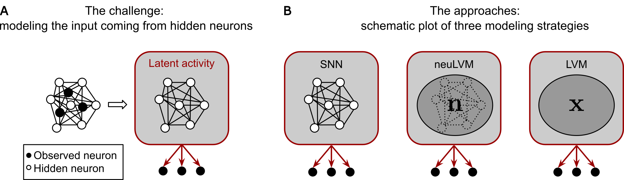
Figure 1: Training SNNs with large numbers of hidden neurons: challenge and approaches. (A) The challenge of modeling the input to the observed neurons (black) coming from the hidden neurons (white) while only a small fraction of neurons is observed. (B) Modeling strategies for the input coming from the hidden neurons: SNNs (left) model the fine-grained spike trains of all hidden neurons; neuLVM (middle) uses a mesoscopic description of the population activity, clustering neurons into homogeneous populations; classic LVMs (right) model the latent activity with low-dimensional phenomenological variables (the link to SNNs is lost).

3 Background: mesoscopic modeling of the population activity

Biophysical neuron models can be accurately approximated (neglecting the nonlinearity of dendritic integration) by simple spiking point neurons [61, 62, 63], which can be efficiently fitted to neural data [64, 65, 66, 67]. Stochastic spiking neuron models where the neuron’s memory of its own spike history is restricted to the time elapsed since its last spike (its age) are said to be of renewal-type. Examples of renewal-type neurons include noisy leaky integrate-and-fire and ‘Spike-Response Model 0’ neurons [9, 10]. The dynamics of a homogeneous population of interacting renewal-type neurons can be described, in the mean-field limit, by an exact integral equation [69, 7, 9, 10, 12] (see [70, 71, 72] for rigorous proofs). In the case of homogeneous but finite populations, Schwalger et al. [11] derived a stochastic integral equation that provides a mesoscopic description (i.e. a description including finite-size fluctuations) of the population dynamics.

For clarity of exposition, in this section and the next, we focus on the case of a single homogeneous population with no external input. All the arguments presented below can be readily generalized to the case of multiple interacting populations with external input (Appendices A B C).

Let us consider a homogeneous SNN of $N$ recurrently connected renewal-type spiking neurons. For $T$ discrete time steps of length $\Delta t$, let $\mathbf{y}\in\{0,1\}^{N\times T}$ (a $N\times T$ binary matrix) denote the spike trains generated by the $N$ neurons. The fact that the neurons are of renewal-type implies, by definition, that the probability for neuron $i$ to emit a spike at time $t$ can be written $p({y}^{i}_{t}=1|{\mathbf{y}}_{1\mathrel{\mathop{\mathchar 58\relax}}t-1},\Theta)=\rho^{\Delta t}_{\theta^{i}}(a^{i},\sum_{j}J^{ij}{\mathbf{y}}^{j}_{1\mathrel{\mathop{\mathchar 58\relax}}t-1})$ where $a^{i}$ is the age of neuron $i$ (i.e. the number of time steps elapsed since the last spike of neuron $i$), the $J^{ij}$ are the recurrent synaptic weights of the network, and $\theta^{i}$ are the parameters of neuron $i$. The sum $\sum_{j}J^{ij}{\mathbf{y}}^{j}_{1\mathrel{\mathop{\mathchar 58\relax}}t-1}$ represents the past input received by neuron $i$ in all time steps up to $t-1$. The superscript $\Delta t$ of the function $\rho^{\Delta t}_{\theta^{i}}$ indicates that we consider here the discrete-time ‘escape rate’ of the neuron but the transition to continuous time is possible [10]. The explicit expression for $\rho^{\Delta t}_{\theta^{i}}$ in the case of leaky integrate-and-fire neurons with ‘escape noise’ (LIF) is given in Appendix A.

A crucial notion in this work is that of a ‘homogeneous population’. The SNN described above forms a homogeneous population if all the recurrent synaptic weights are identical, that is, $J^{ij}=J/N$ (mean-field approximation), and if all the neurons share the same parameters, that is, $\theta^{i}=\theta$. In a homogeneous population, all the neurons share the same past input $J\mathbf{n}_{1\mathrel{\mathop{\mathchar 58\relax}}t-1}/N$, where $\mathbf{n}_{1\mathrel{\mathop{\mathchar 58\relax}}t-1}=(n_{1},n_{2},\dots,n_{t-1})$ denotes the total number of spikes in the population in time steps $1,2,\dots,t-1$ with $n_{t^{\prime}}=\sum_{i=1}^{N}y^{i}_{t^{\prime}}$ being the total number of spikes in the population at time $t^{\prime}$. Then, for any neuron in the population, the probability to emit a spike at time $t$, given its age $a$, is

$$p_{t,a}^{\mathrm{fire}}=\rho^{\Delta t}_{\theta}(a,J\mathbf{n}_{1\mathrel{\mathop{\mathchar 58\relax}}t-1}/N).$$ (1)

Importantly, Eq. (1) is independent of the identity of the neuron.

In a microscopic description of the spiking activity, the vector $\mathbf{y}_{t}$ depends nonlinearly on the past $\mathbf{y}_{1\mathrel{\mathop{\mathchar 58\relax}}t-1}$. A mesoscopic description aims to reduce the high-dimensional microscopic dynamics to a lower-dimensional dynamical system involving the population activity $n_{t}$ only (in the case of multiple interacting populations, $\mathbf{n}_{t}$ is a vector of dimension $K$ equal to the number of populations, Appendix A). While an exact reduction is not possible in general (neuron models being nonlinear), a close approximation in the form of a stochastic integral equation was proposed by Schwalger et al. [11]. In discrete time, the stochastic integral equation reads

$$n_{t} \sim\text{Binomial}\left(N,\;\bar{n}_{t}/N\right),$$ (2a)

$$\bar{n}_{t} =\Bigg{[}\sum_{a\geq 1}p^{\mathrm{fire}}_{t,a}S_{t,a}\,n_{t-a}+\underbrace{\Lambda_{t}\bigg{(}N-\sum_{a\geq 1}S_{t,a}\,n_{t-a}\bigg{)}}_{\text{`finite-size correction'}}\Bigg{]}_{+}.$$ (2b)

The variable $\bar{n}_{t}$ can be interpreted as the expected number of neurons firing at time $t$. The survival $S_{t,a}=\prod_{s=0}^{a-1}(1-p^{\mathrm{fire}}_{t-a+s,s})$ is the probability for a neuron to stay silent between time $t-a$ and $t-1$. The finite-size correction term stabilizes the model by enforcing the approximate neuronal mass conservation $\sum_{a\geq 1}S_{t,a}\,n_{t-a}\approx N$ (see [13] for an in-depth mathematical discussion). The ‘modulating factor’ $\Lambda_{t}$ has an explicit expression [11, 13] in terms of $p^{\mathrm{fire}}$, $S$ and $\mathbf{n}$ (indices are dropped here for simplicity, complete formulas are presented in Appendix A, as well as explanations on how to initialize Eq. (2)). Importantly, for a populations of interacting neurons, $p^{\mathrm{fire}}$, $S$ and $\Lambda$ depend on $\mathbf{n}$, which makes the stochastic equation (2) highly nonlinear. While the mesoscopic model (2) is not mathematically exact, it provides an excellent approximation of the first and second-order statistics of the population activity [11], and is much more tractable than the exact ‘field’ equation [73, 74]. Also, the mesoscopic model (2) can be generalized to the case of non-renewal neurons with spike-frequency adaptation [11] and short-term synaptic plasticity [75].

Formally, Eq. (2) is reminiscent of the Point Process Generalized Linear Model (GLM) [55, 56, 57] for single neurons, with the notable difference that Eq. (2) contains additional nonlinearities beyond those of the GLM because $p^{\mathrm{fire}}$, $S$ and $\Lambda$ all depend on $\mathbf{n}$ (Appendix A). Importantly, Equation (2) readily defines an expression for the probability $p(\mathbf{n}|\Theta)$ [54], where $\Theta=\{J,\theta\}$ denotes the model parameters. Thus, the mesoscopic model (2) allows us to avoid the intractable sum encountered if we naively try to derive $p(\mathbf{n}|\Theta)$ directly from the microscopic description (the intractable sum stems from the fact that the identity of neurons is lost in the observation $n_{t^{\prime}}$ at each time step $t^{\prime}$, Figure 1B).

4 Theoretical result: Neuronally-grounded latent variable model

In this section, we first recall why training SNN with large numbers of hidden neurons via the maximum likelihood estimator is computationally expensive. Then, we show that the mesoscopic description, Eq. (2), allows us to derive a tractable, neuronally-grounded latent variable model, which can be mapped to a multi-population SNN.

For the sake of simplicity, all the arguments are presented for a single homogeneous population, but the generalization to multiple interacting populations is straightforward (Appendices B and C). Let us assume that we observe, during $T$ time steps, the spike trains of $q$ simultaneously recorded neurons that are part of a homogeneous population of $N$ neurons, with $N>q$. We split the spike trains of the entire population $\mathbf{y}\in\{0,1\}^{N\times T}$ into the observed spike trains $\mathbf{y^{o}}$ ($q$ neurons) and hidden spike trains $\mathbf{y^{h}}$ ($N-q$ neurons). Even for a single population, it is difficult to infer the parameters $\Theta=\{J,\theta\}$ of the SNN from observation $\mathbf{y^{o}}$ using the maximum likelihood estimator because, in the presence of hidden neurons, the likelihood $\mathcal{L}$ involves a marginalization over the latent spike trains $\mathbf{y^{h}}$:

$$\mathcal{L}=p(\mathbf{y^{o}}|\Theta)=\sum_{\mathbf{y^{h}}}p(\mathbf{y^{o}},\mathbf{y^{h}}|\Theta).$$ (3)

While different variants of the Expectation-Maximization (EM) algorithm [76] relying on sampling $\mathbf{y^{h}}$ have been used to maximize the likelihood [6, 3, 4], these algorithms scale poorly with the number of hidden neurons.

Instead, we exploit the fact that, for a homogeneous population, the fine-grained knowledge of the latent activity $\mathbf{y^{h}}$ is not necessary since all the observed neurons receive at time $t$ the same input $Jn_{t}$, where $n_{t}=\sum_{i=1}^{N}y^{i}_{t}$ is the population activity of Section 3. Hence, we rewrite the likelihood (3) as

$$\mathcal{L}=p(\mathbf{y^{o}}|\Theta)=\sum_{\mathbf{n}}p(\mathbf{y^{o}},\mathbf{n}|\Theta),$$ (4a)

where the probability $$p(\mathbf{y^{o}},\mathbf{n}|\Theta) T$$ factorizes in terms of the form

$$p(\mathbf{y}^{\mathbf{o}}_{t},n_{t}|\mathbf{y}^{\mathbf{o}}_{1\mathrel{\mathop{\mathchar 58\relax}}t-1},\mathbf{n}_{1\mathrel{\mathop{\mathchar 58\relax}}t-1},\Theta)=\underbrace{p(\mathbf{y}^{\mathbf{o}}_{t}|\mathbf{y}^{\mathbf{o}}_{1\mathrel{\mathop{\mathchar 58\relax}}t-1},\mathbf{n}_{1\mathrel{\mathop{\mathchar 58\relax}}t-1},\Theta)}_{\text{given by neuron model, Eq.~{}\eqref{eq:neuron-model}}}\underbrace{p(n_{t}|\mathbf{n}_{1\mathrel{\mathop{\mathchar 58\relax}}t-1},\Theta)}_{\text{approx. by meso. model, Eq.~{}\eqref{eq:stochastic_integral}}}.$$ (4b)

A comparison of Eqs. (3) and (4) shows that the high-dimensional latent activity $\mathbf{y^{h}}$ has been reduced to a low-dimensional mesoscopic description. Importantly, the $q$ observed spike trains are conditionally independent given the population activity $\mathbf{n}$. While the conditional dependence structure implied by Eq. (4b) is typical of standard latent variable models of multi-neuronal recordings [77, 40, 78, 33], in our approach, the latent variable explicitly represents the population activity of the generative SNN and the parameters of the model are identical to those of the SNN. As the latent population dynamics directly stems from neuronal dynamics, we call our LVM the neuronally-grounded latent variable model (neuLVM).

The nonlinearity and the non-Markovianity of Eq. (2) prevent us from using previous EM algorithms [77, 40, 78, 33]. Therefore, we fit the neuLVM via the Baum-Viterbi algorithm [79] (also known as Viterbi training or hard EM [80]), which alternates estimation (E) and maximization (M) step

1. $\widehat{\mathbf{n}}^{n}=\operatorname{argmax}_{\mathbf{n}}\log p(\mathbf{y^{o}},\mathbf{n}|\widehat{\Theta}^{n-1})$,

2. $\widehat{\Theta}^{n}=\operatorname{argmax}_{\Theta}\log p(\mathbf{y^{o}},\widehat{\mathbf{n}}^{n}|\Theta)$.

The estimated parameters $\widehat{\Theta}$ and the estimated latent population activity $\widehat{\mathbf{n}}$ are the result of many iterations of E-step and M-step (Appendix C). Note that the computational cost of this algorithm does not depend on the number of hidden neurons (it only depends on the number of populations)..

5 Experimental results

5.1 Single homogenous population: SNN with metastable cluster states

Although seemingly simple, homogeneous populations of leaky integrate-and-fire (LIF) neurons without external stimulation are SNNs with a rich repertoire of population dynamics, including asynchronous states, synchronous states, and cluster states [7, 9]. In a $m$-cluster state (with $m\geq 2$), the population activity oscillates at a frequency $m$ times higher than the average neuronal firing rate: a neuron spikes every $m$ cycle on average; conversely, approximately $N/m$ neurons fire in each cycle ($N$ being to the total number of neurons). Cluster states have therefore been described as ‘higher harmonics’ of the synchronous state (or $1$-cluster state) [81, 82, 83, 9] where all neurons fire in synchrony.

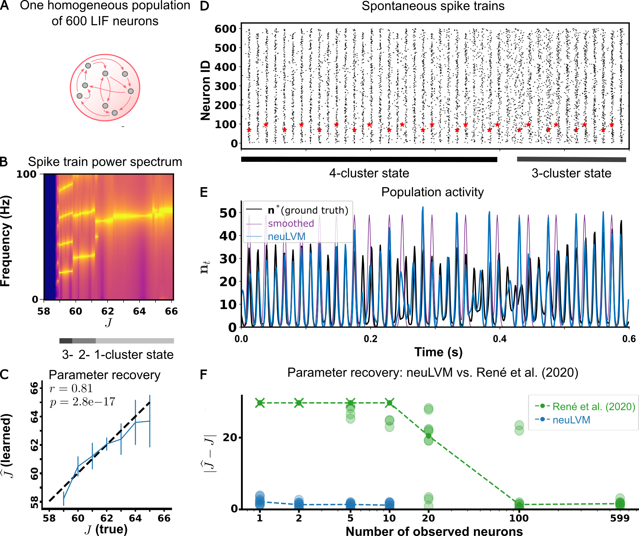
Figure 2: Single-population SNN with metastable cluster states. (A) Network architecture (for visualization purposes, only a few connections are drawn). (B) Spike train power spectrum for different choices of connectivity parameter $J$. All simulations start from the same unstable asynchronous state. The corresponding cluster states are indicated below. The blue region around $J=58$ mV indicates the absence of activity. (C) Connectivity recovered by the neuLVM $\widehat{J}$ vs ground truth $J$. The neuLVM was fitted on one-second single-trial recordings of six neurons ($1\%$ of the population). For each ground truth $J$ value (seven in total), ten different trials were generated: bars indicate the standard deviations of the recovered $\widehat{J}$. The Pearson correlation coefficient between the recovered $\widehat{J}$ and $J$ is $r=0.81$ and the associated p-value is $2.8\mathrm{e}{-17}$ (see Table S3). (D) Spike trains generated by the ground truth SNN for a trial showing a transition from a metastable $4$-cluster state to a $3$-cluster state. The spike trains of two randomly sampled neurons (red stars) formed the training data (for visualization purposes, only the first $0.6$ second of the one-second trial is shown) on which neuLVM was fitted: (E) the inferred population activity $\widehat{\mathbf{n}}|\mathbf{y^{o}}$ is compared to the ground truth $\mathbf{n}^{*}$ and the summed, smoothed spike trains (Gaussian smoothing window with $\sigma=1.4$ ms, Appendix D) of the two observed neurons. (F) Absolute difference between the recovered $\widehat{J}$ and the ground truth $J$ for the neuLVM algorithm and the method of René et al. (2020) for varying numbers of observed neurons. Using the same trial as in D, for each number of observed neurons, the two methods were tested on $10$ different samples of observed neurons (see Table S4). The marker ‘$\times$’ indicates that the difference $|\widehat{J}-J|$ is larger than $30$ mV. The median samples are linked with dashed lines to show the trends.

In this set of experiments, we always consider the same network of $600$ LIF neurons (Figure 2A), where only the connectivity parameter $J$ varies. When initialized at time $0$ in the same unstable asynchronous state, the network can spontaneously settle in a $m$-cluster state, where $m$ depends on the recurrent connectivity parameter $J$ (Figure 2B): finite-size fluctuations break the symmetry of the asynchronous state and the population splits into $m$ groups of synchronized neurons. The cluster state to which the network converges can be read from the power spectrum of the neuronal spike trains (Figure 2B) (the fundamental frequency of the $m$-cluster state is approximately $m$ times lower than that of the $1$-cluster state). Generating spike trains for $6$ observed neurons ($1\%$ of the population), we tested whether neuLVM could recover the connectivity parameter $J$ (neuronal parameters $\theta$ were given), for different $J$’s in the $1$-, $2$-, and $3$-cluster states range (Figure 2C, Table S3). The Pearson correlation between the learned $\widehat{J}$ and the true $J$ was $0.81$ with p-value $2.8\mathrm{e}{-17}$, showing that, statistically, neuLVM could recover the connectivity parameter of the SNN.

To assess how well neuLVM can infer the latent population activity and how neuLVM compares with the methods assuming full observability (like René et al. [54]), we studied in detail a single trial showing a transition from a metastable $4$-cluster state to a $3$-cluster state (Figure 2D,E). To generate this trial, we chose $J=60.32$ mV and initialized the network in the $4$-cluster state. From the spike trains of only two neurons (red stars in Figure 2D), neuLVM could infer the ground truth population activity $\mathbf{n}^{*}$ during the $4$-cluster state, and during the $3$-cluster state, and could approximately detect the transition between the two states (Figure 2E). While the summed, smoothed spike trains missed two out of four population activity peaks in the $4$-cluster state, and one out of three peaks in the $3$-cluster state (purple curve in Figure 2E), the strong inductive biases contained in neuLVM enabled the inference of the ‘missing’ peaks (blue curve in Figure 2E). Finally, neuLVM and a method assuming full observability (equivalent to a naive application of René et al. [54]) were compared through their ability to recover the connectivity parameter $J$, for varying numbers of observed neurons (Figure 2F, Table S4). Since a naive application of the method of René et al. [54] does not take into account hidden neurons, it led, as expected, to wildly inaccurate estimates $\widehat{J}$ when the summed spike train was far from the ground truth population activity (which happened when the number of observed neurons was small, see Figure 2E for an example). In contrast, the neuLVM managed to recover the connectivity parameter, thanks to the fact that the Baum-Viterbi algorithm of Section 4 also infers the population activity (see Figure 2E for an example).

5.2 Multiple populations: SNN with metastable point attractors

5.2.1 Latent population activity inference and reproduction of metastable dynamics

As a second benchmark, we tested neuLVM on synthetic data generated by three interacting populations with two populations of $400$ excitatory LIF neurons and one population of $200$ inhibitory neurons (Figure 3A). Recurrent connections between these population drive winner-take-all dynamics with finite-size fluctuations-induced switches of activity between the two excitatory populations [11, 84] – an example of ‘itinerancy between attractor states’ [25]. The population activities of this metastable, three-population SNN constitute the ground truth against which different models will be tested.

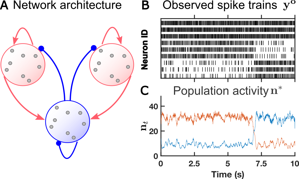
Figure 3: Network architecture and example trial. (A) Architecture of the three-population, metastable, winner-take-all SNN. (B) Example trial from the spiking benchmark dataset: 10 seconds recordings of $9$ observed neurons ($3$ neurons from each of the three populations) and (C) corresponding ground truth latent population activity (for the two excitatory populations).

To build a spiking benchmark dataset, we randomly selected $9$ neurons – $3$ neurons from each of the three populations – and considered the spike trains of these neurons as the observed data. For simplicity, the correct partitioning of the $9$ neurons into $3$ groups is given since it can be reliably obtained by k-means clustering [85] using the van-Rossum-Distance [86] between spike trains. The complete dataset consists of $20$ trials of $10$ seconds. An example trial is shown in Figure 3B.

In contrast with the experiments of Section 5.1 where the neuronal parameters were given, here, neuronal and connectivity parameters are not given to neuLVM (see Appendix F). We compared the performance of neuLVM with other generative models of spiking data – PLDS [33], SLDS [39], and GLM [55, 56, 57] – on single trials of the spiking benchmark dataset in two ways: (i) we measured the Pearson correlation $r$ between the inferred latent population activity $\widehat{\mathbf{n}}|\mathbf{y}^{\mathbf{o}}$ and the ground truth population activity $\mathbf{n}^{*}$ (Table 1 first column); (ii) we assessed how well could the fitted models reproduce metastable dynamics by counting the occurrences of stochastic switches in free simulations – or in other words, samples – of the fitted models (Table 1 second column). Tests (i) and (ii) on an example trial are shown in Figure 4.

The Poisson Linear Dynamical Systems approach (PLDS, [33]) assumes that the recorded spikes can be explained by point processes driven by a latent linear dynamical system of low dimension. The Poisson Switching Linear Dynamical System (SLDS, [34, 35, 36, 37, 38, 39]) extends PLDS by allowing the latent variables to switch randomly between two dynamical systems with distinct parameters. We should stress that, in PLDS and SLDS, the latent variables are phenomenological representations of neural population activity which have no direct link with the ground truth population activity $\mathbf{n}^{*}$. In order to still make test (i) possible for PLDS and SLDS, we will consider the best linear transformation of the inferred latent variables which minimizes the mean squared error with the ground truth population activity $\mathbf{n}^{*}$.

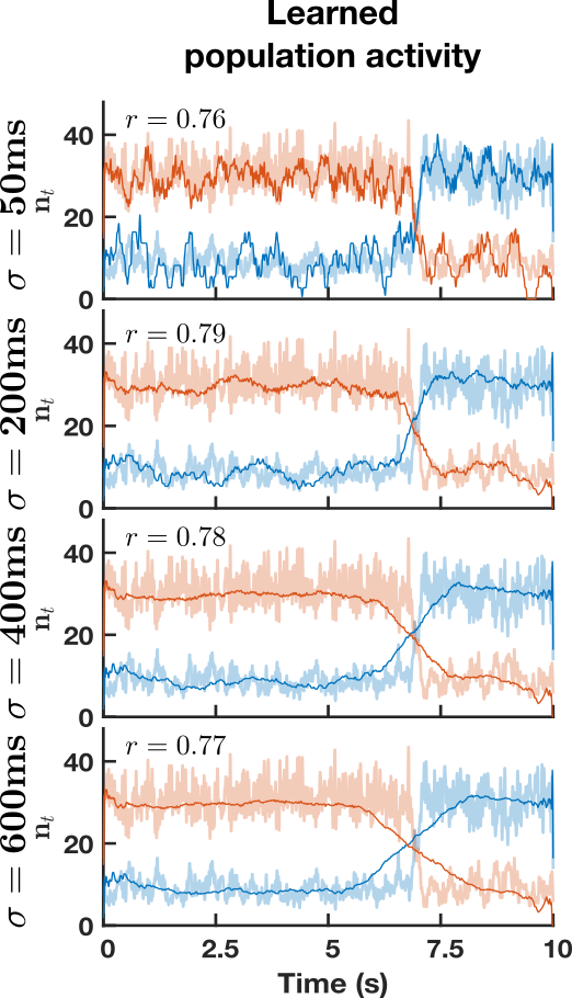
Figure S6: Smoothed empirical estimate $\widehat{\mathbf{n}}^{\mathrm{sm},\alpha}_{\sigma,t}$ (Appendix D) of the latent population activity for one example trial (the same as in Figure 3, two excitatory populations). The value $r$ is the Pearson correlation coefficient between the inferred $\widehat{\mathbf{n}}|\mathbf{y^{o}}$ and the ground truth $\mathbf{n}^{*}$ population activities.

On test (i), neuLVM gave better estimates $\widehat{\mathbf{n}}|\mathbf{y}^{\mathbf{o}}$ of the latent population activity $\mathbf{n}^{*}$ (Pearson correlation $r=0.81$) than the best linear transformation of the latent activity inferred by PLDS and SLDS ($r=0.69$ and $r=0.73$ respectively) (Table 1 first column). The GLM approach cannot be included in test (i) since it ignores unobserved neurons. Interestingly, the example trial in Figure 4A shows the latent population activity $\widehat{\mathbf{n}}|\mathbf{y}^{\mathbf{o}}$ inferred by neuLVM is smoother than the ground truth $\mathbf{n}^{*}$ before and after the switch (finite-size fluctuations are reduced) but $\widehat{\mathbf{n}}|\mathbf{y}^{\mathbf{o}}$ and $\mathbf{n}^{*}$ closely match around the time of the switch. In contrast, fluctuations are exaggerated for PLDS and SLDS. The population activity estimated by simply summing and smoothing the observed spike trains (Appendix D) is shown in Figure S6.

On test (ii), neuLVM, fitted on a single trial of $10$ seconds, was able to reproduce stochastic switches similar to that of the ground truth SNN (Table 1 second column): free simulations of the fitted neuLVM showed $7.8$ switches in $100$ seconds on average ($10.3$ switches on average for the ground truth SNN). To make sure that stochastic switches were the result of parameter learning via the Baum-Viterbi algorithm, we verified that, before learning, neuLVM did not show any metastable dynamics (Figure S7). Examples of simulated trials are shown in Figure 4B. PLDS failed to reproduce stochastic switches, which is not surprising since winner-take-all dynamics are typically nonlinear. SLDS could reproduce stochastic switches at the correct mean frequency ($11.9$ instead of the ground truth $10.3$), but the standard deviation of the simulated switch count, $8.9$ ($2.7$ for the ground truth SNN), indicates that a single $10$ seconds trial was probably not sufficient for SLDS to learn switching probabilities reliably. Finally, neuronal stochasticity and small network size ($9$ neurons) did not allow GLM to produce stochastic switches, even when the training trial was prolonged to $500$ seconds.

Taken together, only neuLVM could infer the latent population activity and reliably learn the metastable dynamics on single trials of $10$ seconds, demonstrating the effectiveness of its neuronally-grounded inductive biases. Of course, these results do not guarantee that the inductive biases of neuLVM would be effective on real data since real data is most certainly out-of-distribution for neuLVM. While applications on real data are beyond the scope of this paper, in Appendix F, we show that neuLVM is robust, to a certain extent, to within-population heterogeneity and out-of-distribution data.

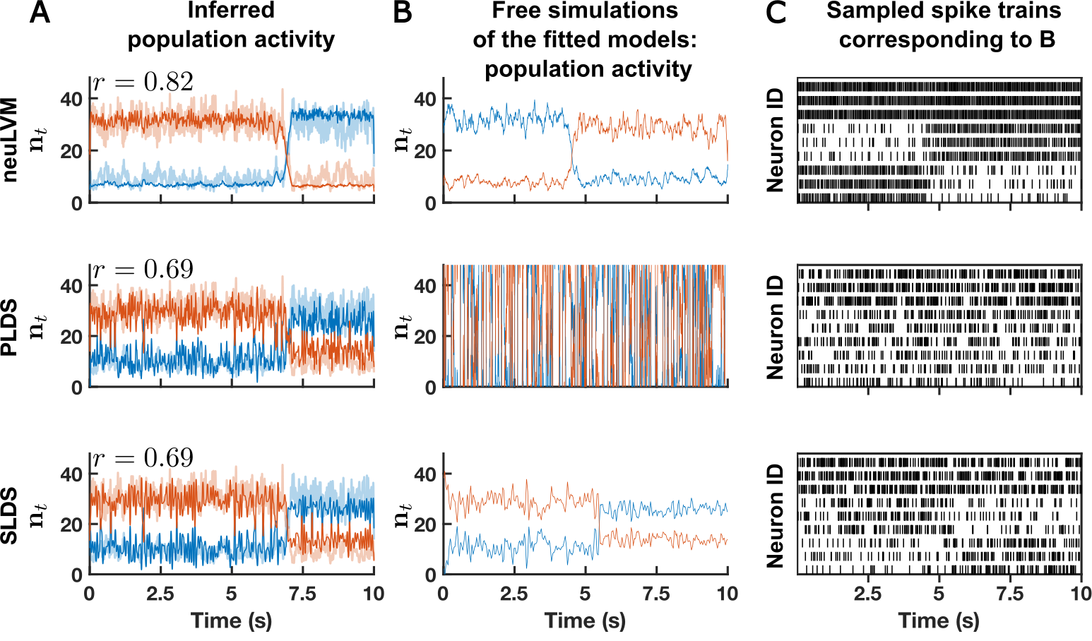
Figure 4: Three-population SNN with metastable point attractors. (A) Latent population activity of the two excitatory populations inferred by neuLVM / PLDS / SLDS for one example trial (the same as in Figure 3). The value $r$ is the Pearson correlation coefficient between the inferred $\widehat{\mathbf{n}}|\mathbf{y^{o}}$ and the ground truth $\mathbf{n}^{*}$ population activities. (B-C) Examples of free simulations of the fitted neuLVM / PLDS / SLDS.

Table 1: Model performance summary (corresponding to Figure 4).

Models	Pearson correlation $r$ between $\widehat{\mathbf{n}}|\mathbf{y^{o}}$ and $\mathbf{n}^{*}$	Number of switches during $100$ seconds free simulations of the fitted models ($10.3\pm 2.7$ for the ground truth SNN)
neuLVM	$0.81\pm 0.02$	$7.8\pm 4.1$
PLDS	($0.68\pm 0.11$)	not visible
SLDS	($0.73\pm 0.02$)	$11.9\pm 8.9$
GLM	-	not visible

Mean and ($\pm$) standard deviation were computed over $20$ different trials. Parentheses for PLDS and SLDS indicate that these results are for the best linear transformation of the inferred latent variables.

5.2.2 Generalization: towards experimental predictions with neuronally-grounded modeling

Bottom-up, mechanistic models allow us to perform in silico experiments and generate predictions about neural microcircuits, which can then be tested experimentally. So we wondered: can neuLVM, fitted on a single trial of spontaneous activity (like in Section 5.2.1), predict the response of the SNN when an external perturbation is applied? As a preliminary step in that direction, we tested whether an external stimulation of the fitted model would generate the same response as that of the microscopic SNN when subjected to the same perturbation.

Using the same multi-population network as in Section 5.2 (Figure 3A) and neuLVM fitted on a single trial of spontaneous activity (Figure 3B), we compared the response of the ground truth SNN with that of neuLVM when one of the populations was stimulated by a current pulse of $4$ ms mimicking the stimulation of an optogenetically modified population by a short light pulse. We simulated $100$ trials where the momentarily active excitatory population was stimulated, and 100 where the momentarily silent excitatory population was stimulated (Figure 5A and B respectively). Each stimulation led to two possible outcomes: stimulation could trigger a state switch (Switch trials) or no state switch (No-switch trials). In both the ground truth SNN and the fitted neuLVM, we found that stimulating the silent population triggered more frequent state switches (Figure 5B) than stimulating the active population (Figure 5A). Moreover, in both the ground truth and the fitted neuLVM, we could induce ‘excitatory rebound’ switches by stimulating the active population (Figure 5A, lower half).

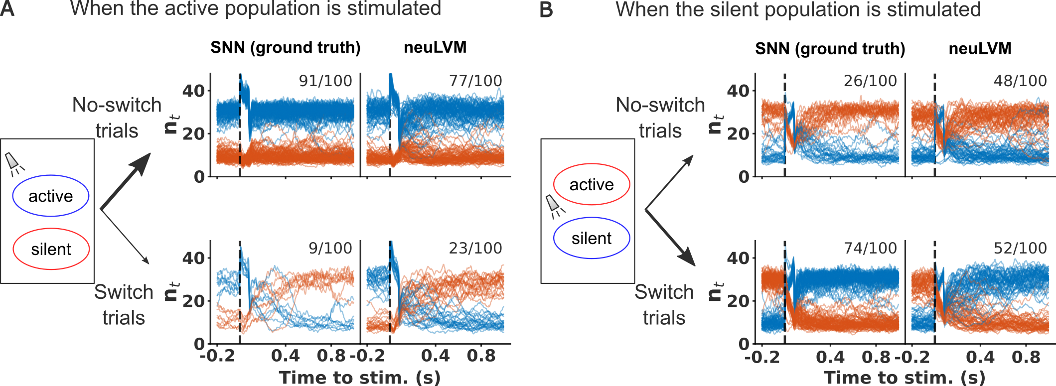
Figure 5: Network responses to perturbations mimicking optogenetic stimulation. (A) Activities of the excitatory populations when the active population is stimulated ($100$ trials, ratios indicate the number of No-switch or Switch trials). (B) Same as A but the silent population is stimulated.

6 Discussion

Understanding the neural dynamics underlying computation in the brain is one of the main goals of latent variable modeling of multi-neuronal recordings [87, 45, 47, 51, 53, 88]. We contribute to this effort by proposing here a bottom-up, mechanistic LVM – the neuronally-grounded latent variable model (neuLVM) – which can be mapped to a multi-population SNN. Using SNN-based generative models, which are more biological than RNN-based models [45], could allow systems neuroscientists to test hypotheses about the architecture of the probed microcircuit, and provide a neuronally-grounded understanding of computation.

While this work shows the potential of the neuLVM approach, the application of neuLVM to real data faces two methodological challenges. First, there is the problem of identifiability: although neuLVM could recover a single unknown connectivity parameter (Section 5.1), our method could not always recover the SNN parameters when many parameters were unknown (Section 5.2). Bayesian inference could circumvent the problem of non-identifiability by estimating the full posterior distribution over model parameters [89, 54]. In addition, perturbing the probed network, with optogenetic stimulation, for example, could help model parameter recovery by providing richer data. Second, in the case of real data, choosing a good generative SNN model is a nontrivial task. For example, how many homogeneous populations should the SNN have? Clustering the recorded spike trains could guide the design of possible generative models and Bayesian model comparison, as used in biophysical modeling of neuroimaging data [90, 91, 92], could help in selecting the most likely model among several possible models.

The model proposed here is only one particular example of an SNN-based, tractable latent variable model. Whether other such neuronally-grounded models of partially observed spike trains can be formulated and efficiently applied to real data is a question left for future work.

Appendix A Mesoscopic model in the case of LIF neurons

In this section, we present in detail the mesoscopic model of SchDeg17 in the case of multiple interacting populations of LIF neurons, as formulated in SchLoe21.

Fine-grained SNN of LIF neurons with escape noise.

Let us consider a general network of $N$ LIF neurons (indexed by $i=1,\dots,N$) with escape noise GerKis14. Neurons are modeled as point processes: the probability for neuron $i$ to emit a spike at time $t$, given the past network activity ${\mathbf{y}}_{1\mathrel{\mathop{\mathchar 58\relax}}t-1}$, is

$$p({y}^{i}_{t}=1|{\mathbf{y}}_{1\mathrel{\mathop{\mathchar 58\relax}}t-1},\Theta)=1-\exp\left(-\lambda^{i}_{t}\Delta t\right),\quad\text{with }\lambda^{i}_{t}=\exp\left(V^{i}(t|\hat{t}^{i})-\vartheta^{i}\right),$$

where the escape rate (or stochastic intensity) $\lambda^{i}_{t}$ depends on the momentary difference between the membrane potential $V^{i}(t|\hat{t}^{i})$ and the firing threshold $\vartheta^{i}$, via an exponential escape function. The voltage $V^{i}(t|\hat{t}^{i})$ of neuron $i$ at time $t$ depends on its last spike time $\hat{t}^{i}=t-a^{i}$ and the inputs received up to time $t$, which include the inputs coming from the other neurons and the external input $\mathbf{I}^{\mathrm{ext},i}_{1\mathrel{\mathop{\mathchar 58\relax}}t}$. Between spikes, for all $t>\hat{t}^{i}+t^{i}_{\mathrm{ref}}$ ($t^{i}_{\mathrm{ref}}$ being the absolute refractory period of neuron $i$), the voltage dynamics follows

$$V^{i}(t|\hat{t}^{i}) =V^{i}(t-1|\hat{t}^{i})+\left(\frac{U^{i}_{\mathrm{r}}+RI^{\mathrm{ext},i}_{t}-V^{i}(t-1|\hat{t}^{i})}{\tau^{i}_{\mathrm{mem}}}\right)\Delta t+\sum_{j=1}^{N}J^{ij}\left(\epsilon^{ij}*\mathbf{y}^{j}\right)(t),$$

and $V^{i}(t|\hat{t}^{i})=0$, for all $t\leq\hat{t}^{i}+t^{i}_{\mathrm{ref}}$ (which means that the voltage is reset to $0$ after each spike and is clamped at $0$ for an absolute refractory period $t^{i}_{\mathrm{ref}}\geq 0$). The parameters $\tau^{i}_{\mathrm{mem}}>0$ and $U^{i}_{\mathrm{r}}>0$ are the membrane time constant and the resting potential respectively. The neuron $i$ is therefore characterized by the parameters $\theta^{i}=\{\vartheta^{i},U^{i}_{\mathrm{r}},\tau^{i}_{\mathrm{mem}},t^{i}_{\mathrm{ref}}\}$. While the escape function is usually parameterized by a rescaled exponential function of the form $f(v)=\frac{1}{\tau^{i}_{0}}\exp(\beta^{i}(v-\tilde{\vartheta}^{i}))$ [Sec 9.1]GerKis14, the parameters $\tau^{i}_{0},\beta^{i}$ and $\tilde{\vartheta}^{i}$ can be absorbed in $\vartheta^{i}$ (up to a rescaling of the resting potential $U^{i}_{\mathrm{r}}$). The resistance $R=1\,\Omega$ is used here simply for the consistency of physical units. The postsynaptic current induced by a spike of neuron $j$ on neuron $i$ is defined by the synaptic weight $J^{ij}$ and the synaptic kernel $\epsilon^{ij}\mathrel{\mathop{\mathchar 58\relax}}\mathbb{R}_{+}\to\mathbb{R}_{+}$. In this work, we consider exponential kernels of the form $\epsilon^{ij}(t)=\frac{\mathcal{H}(t-\Delta^{ij})}{\tau^{ij}_{\mathrm{syn}}}\exp\left(-\frac{t-\Delta^{ij}}{\tau^{ij}_{\mathrm{syn}}}\right)$, where $\tau^{ij}_{\mathrm{syn}}$ is the synaptic time constant, $\Delta^{ij}$ is the synaptic delay and $\mathcal{H}$ is the Heaviside function. The symbol $\ast$ denotes the convolution operator.

Coarse-grained multi-population SNN.

Coarse-graining and mean-field approximations consist in partitioning the $N$ neurons into $K$ homogeneous populations, indexed by $\alpha=1,\dots,K$, where (i) all the neurons $i$ in population $\alpha$ share the same neuronal parameters $\theta^{i}=\theta^{\alpha}$; (ii) for any neuron $j$ in population $\beta$ and any neuron $i$ in population $\alpha$, $J^{ij}=J^{\alpha\beta}/N^{\beta}$ ($N^{\beta}$ being the number of neurons in population $\beta$) and $\epsilon^{ij}=\epsilon^{\alpha\beta}$; (iii) all the neurons $i$ in population $\alpha$ share the same external input $\mathbf{I}^{\mathrm{ext},i}=\mathbf{I}^{\mathrm{ext},\alpha}$. In such a coarse-grained $K$-population SNN, we have, for any neuron $i$ in population $\alpha$,

$$\sum_{j=1}^{N}J^{ij}\left(\epsilon^{ij}*\mathbf{y}^{j}\right)(t)=\sum_{\beta=1}^{K}J^{\alpha\beta}\left(\epsilon^{\alpha\beta}*\mathbf{n}^{\beta}\right)(t)/N^{\beta},$$

where $n^{\beta}_{t}=\sum_{i\,\in\,\text{pop. $\beta$}}y^{i}_{t}$ is the total number of spikes in population $\beta$ at time $t$. Hence, the probability for any neuron $i$ in population $\alpha$ to emit a spike at time $t$, given its age $a$ and the past population activity $\mathbf{n}_{1\mathrel{\mathop{\mathchar 58\relax}}t-1}$ is

$$p_{t,a}^{\mathrm{fire},\alpha}=1-\exp\left(-\lambda^{\alpha}_{t}\Delta t\right),\quad\text{with }\lambda^{\alpha}_{t}=\exp\left(V^{\alpha}(t|t-a)-\vartheta^{\alpha}\right).\\$$ (5)

For all $a>t^{\alpha}_{\mathrm{ref}}$, we have the update rule

$$V^{\alpha}(t|t-a)=V^{\alpha}(t-1|t-a)+\left(\frac{U^{\alpha}_{\mathrm{r}}+RI^{\mathrm{ext},\alpha}_{t}-V^{\alpha}(t-1|t-a)}{\tau^{\alpha}_{\mathrm{mem}}}\right)\Delta t\\ +\sum_{\beta=1}^{K}J^{\alpha\beta}\left(\epsilon^{\alpha\beta}*\mathbf{n}^{\beta}\right)(t)/N^{\beta},$$

and $V^{\alpha}(t|t-a)=0$ for all $a\leq t^{\alpha}_{\mathrm{ref}}$. This gives the explicit expression for the probability $p_{t,a}^{\mathrm{fire}}$ in Eq. (1). In this work, for simplicity, we will assume that all the synaptic kernels are the same, i.e. $\epsilon^{\alpha\beta}=\epsilon$, $\forall\alpha,\beta$ (see Table S2).

Mesoscopic description.

The $K$-population SNN described above does not by itself constitute a mesoscopic model because the probability $p_{t,a}^{\mathrm{fire},\alpha}$ still involves the age $a$ of some neuron. To get a mesoscopic model (i.e. a model that does not involve the fine-grained modeling of each individual neuron), SchDeg17 used the population activity $\mathbf{n}$ to approximate the age density of each population and derived a closed-form system of stochastic integral equations: For all $\alpha\in 1,\dots,K$,

$$n^{\alpha}_{t} \sim\text{Binomial}\left(N^{\alpha},\;\bar{n}^{\alpha}_{t}/N^{\alpha}\right),$$ (6a)

$$\bar{n}^{\alpha}_{t} =\Bigg{[}\sum_{a\geq 1}p^{\mathrm{fire},\alpha}_{t,a}S^{\alpha}_{t,a}\,n^{\alpha}_{t-a}+\Lambda^{\alpha}_{t}\bigg{(}N^{\alpha}-\sum_{a\geq 1}S^{\alpha}_{t,a}\,n^{\alpha}_{t-a}\bigg{)}\Bigg{]}_{+},$$ (6b)

$$\Lambda^{\alpha}_{t} =\frac{\sum_{a\geq 1}p^{\mathrm{fire},\alpha}_{t,a}(1-S^{\alpha}_{t,a})S^{\alpha}_{t,a}\,n^{\alpha}_{t-a}}{\sum_{a\geq 1}(1-S^{\alpha}_{t,a})S^{\alpha}_{t,a}\,n^{\alpha}_{t-a}},$$ (6c)

where $S^{\alpha}_{t,a}=\prod_{s=0}^{a-1}(1-p^{\mathrm{fire},\alpha}_{t-a+s,s})$ is the survival, i.e. the probability for a neuron in population $\alpha$ to stay silent between time $t-a$ and $t-1$. A concise version of the derivation of the mesoscopic model (6) is presented in SchLoe21. Note that Eq. (6) is not a one-dimensional stochastic dynamical system: the Markov embedding of the stochastic dynamics (6) is infinite-dimensional SchLoe21. Indeed, Eq. (6) does not only describes the evolution of the population activity $n_{t}^{\alpha}$ but it also describes the evolution of the whole age (pseudo) density $\{S_{t,a}^{\alpha}n_{t-a}\}_{a\geq 1}$ in the population, also called the “refractory density” SchChi19.

Formally, the ‘initial condition’ of Eq. (6) is defined by the population activity $\mathbf{n}_{t}$ for all $t\leq 0$ (denoted $\mathbf{n}_{t\leq 0}$). Several practical choices of initial conditions have been discussed in SchDeg17,RenLon20,SchLoe21. In this work, if not otherwise specified, $\mathbf{n}_{t\leq 0}$ is taken to be time-invariant, with stationary activities estimated from the observed data (see below).

The size of the discrete time steps $\Delta t$ does not need to be the same for the fine-grained SNN and for the mesoscopic model (6). Indeed, it can be useful to take longer time steps for the mesoscopic description (time coarse-graining). In the following appendices, when there is an ambiguity, $\Delta t_{\mathrm{meso}}$ will denote the time step length for the mesoscopic model and neuLVM. The length $\Delta t_{\mathrm{meso}}$ will always be smaller or equal to the neuronal absolute refractory periods so that a neuron can fire at most once in each time step.

Appendix B neuLVM for multiple interacting populations

Let us assume that we observe, during $T$ time steps, the spike trains of $q$ simultaneously recorded neurons that are part of a $K$-population SNN of $N$ neurons, with $N>q$. For each of the population $\alpha=1,\dots,K$, $q^{\alpha}>0$ neurons are observed $(\sum_{\alpha=1}^{K}q^{\alpha}=q)$ and share the same set of neuronal parameters $\theta^{\alpha}$, input weights $\{J^{\alpha\beta}/N^{\beta}\}_{\beta=1}^{K}$, and output weights $\{J^{\beta\alpha}/N^{\alpha}\}_{\beta=1}^{K}$, where $N^{1},\dots,N^{K}$ are the numbers of neurons in each population $(\sum_{\alpha=1}^{K}N^{\alpha}=N)$.

The likelihood $\mathcal{L}$ of the observed spike trains.

Following the assumptions described above, the likelihood $\mathcal{L}$ of the observed spike trains $\mathbf{y^{o}}$ (a binary $q\times T$ matrix) can be formally written as $\sum_{\mathbf{n}}p(\mathbf{y^{o}},\mathbf{n}|\Theta)$, where $\mathbf{n}$ (an integer-valued $K\times T$ matrix) is the population activity and $\Theta=\{\{J^{\alpha\beta}\}_{1\leq\alpha,\beta\leq K},\{\theta^{\alpha}\}_{\alpha=1}^{K}\}$ are the parameters of the $K$-population SNN. The probability $p(\mathbf{y^{o}},\mathbf{n}|\Theta)$ factorizes in $T$ terms of the form

$$p(\mathbf{y}^{\mathbf{o}}_{t},\mathbf{n}_{t}|\mathbf{y}^{\mathbf{o}}_{1\mathrel{\mathop{\mathchar 58\relax}}t-1},\mathbf{n}_{1\mathrel{\mathop{\mathchar 58\relax}}t-1},\Theta)=\underbrace{p(\mathbf{y}^{\mathbf{o}}_{t}|\mathbf{y}^{\mathbf{o}}_{1\mathrel{\mathop{\mathchar 58\relax}}t-1},\mathbf{n}_{1\mathrel{\mathop{\mathchar 58\relax}}t-1},\Theta)}_{\text{{part a}}}\underbrace{p(\mathbf{n}_{t}|\mathbf{n}_{1\mathrel{\mathop{\mathchar 58\relax}}t-1},\Theta)}_{\text{{part b}}}.$$

The probability (part a) of the observed spikes $\mathbf{y}^{\mathbf{o}}_{t}$ at time $t$ given the past observed spike activity $\mathbf{y}^{\mathbf{o}}_{1\mathrel{\mathop{\mathchar 58\relax}}t-1}$ and the past population activity $\mathbf{n}_{1\mathrel{\mathop{\mathchar 58\relax}}t-1}$ is

$$p(\mathbf{y}^{\mathbf{o}}_{t}|\mathbf{y}^{\mathbf{o}}_{1\mathrel{\mathop{\mathchar 58\relax}}t-1},\mathbf{n}_{1\mathrel{\mathop{\mathchar 58\relax}}t-1},\Theta)=\prod_{\alpha=1}^{K}\prod_{i=1}^{q^{\alpha}}p(y^{\mathbf{o},\alpha,i}_{t}|a^{i},\mathbf{n}_{1\mathrel{\mathop{\mathchar 58\relax}}t-1},\Theta)=\prod_{\alpha=1}^{K}\prod_{i=1}^{q^{\alpha}}p_{t,a^{i}}^{\mathrm{fire},\alpha},$$

where $p_{t,a^{i}}^{\mathrm{fire},\alpha}$, given by Eq. (5) in Appendix A, is the probability for the recorded neuron $i$ of population $\alpha$ to emit a spike at time $t$.

The probability (part b) of the population activity $\mathbf{n}_{t}$ at time $t$ given the past population activity $\mathbf{n}_{1\mathrel{\mathop{\mathchar 58\relax}}t-1}$ is

$$p(\mathbf{n}_{t}|\mathbf{n}_{1\mathrel{\mathop{\mathchar 58\relax}}t-1},\Theta)=\prod_{\alpha=1}^{K}p(n^{\alpha}_{t}|\mathbf{n}_{1\mathrel{\mathop{\mathchar 58\relax}}t-1},\Theta),$$

where $p(n^{\alpha}_{t}|\mathbf{n}_{1\mathrel{\mathop{\mathchar 58\relax}}t-1},\Theta)$ is approximated by the mesoscopic model (6).

Appendix C Fitting algorithm for neuLVM

Baum-Viterbi algorithm.

Given the observed spike trains $\mathbf{y^{o}}$, we optimize the likelihood $\mathcal{L}=\sum_{\mathbf{n}}p(\mathbf{y^{o}},\mathbf{n}|\Theta)$ via an EM-like algorithm – the Baum-Viterbi algorithm EphMer02. Relying on the heuristic that the posterior $p(\mathbf{n}|\mathbf{y^{o}},\Theta)$ should be concentrated around its maximum, we approximate the posterior $p(\mathbf{n}|\mathbf{y^{o}},\Theta)$ by a point mass $\delta_{\mu}$, where $\mu=\operatorname*{arg\,max}_{\mathbf{n}}\log p(\mathbf{y^{o}},\mathbf{n}|\Theta)$. By doing so, the alternating estimation (E) and maximization (M) step of the $n$-th iteration read

1. $\widehat{\mathbf{n}}^{n}=\operatorname{argmax}_{\mathbf{n}}\log p(\mathbf{y^{o}},\mathbf{n}|\widehat{\Theta}^{n-1})$,

2. $\widehat{\Theta}^{n}=\operatorname{argmax}_{\Theta}\log p(\mathbf{y^{o}},\widehat{\mathbf{n}}^{n}|\Theta)$.

Details of the optimization.

In the M-step, parameters $\Theta$ are optimized using the L-BFGS-B algorithm and the optimization stops when either the maximum number of iterations ($\text{maxiter}_{\text{M}}$) is reached, or the objective function improves by less than $\text{ftol}_{\text{M}}$, or the maximum norm of the gradient is less than $\text{gtol}_{\text{M}}$. Hyper-parameters including $\text{maxiter}_{\text{M}}$, $\text{ftol}_{\text{M}}$ and $\text{gtol}_{\text{M}}$ are given in Table S5. In the E-step, to carry out gradient ascent, we approximate the discrete Binomial distribution Eq. (6a) by a Gaussian, i.e. $n_{t}^{\alpha}\sim\mathcal{N}\left(\bar{n}_{t}^{\alpha},\bar{n}_{t}^{\alpha}\right)$, where $\bar{n}_{t}^{\alpha}$ is given by the mesoscopic model Eq (6) SchDeg17. With this approximation, the latent population activity $\mathbf{n}$ is optimized with the Adam algorithm with learning rate $\text{lr}_{\text{E}}$ and the optimization stops when either the maximum number of iterations ($\text{maxiter}_{\text{E}}$) is reached, or the objective function stops improving for the last $\text{itertol}_{\text{E}}$ iterations. Hyper-parameters including $\text{lr}_{\text{E}}$, $\text{maxiter}_{\text{E}}$ and $\text{itertol}_{\text{E}}$ are given in Table S5. The estimated parameters $\widehat{\Theta}$ and the estimated latent population activity $\widehat{\mathbf{n}}$ are the result of many iterations of E-step and M-step. The fitting algorithm ends either when it stops improving the objective function or the maximum number of E-M iterations is reached.

Multiple data-driven initializations.

To deal with the fact that the joint probability $p(\mathbf{y^{o}},\mathbf{n}|\Theta)$ to optimize is non-convex and high-dimensional ($\mathbf{n}$ has dimension $K\times T$), we perform the Baum-Viterbi algorithm $\text{N}_{\text{init}}$ times with initial parameters $\widehat{\Theta}^{0}$ uniformly sampled in a certain range given in Appendices E and F. Since the sum over the observed neurons from population $\alpha$, $\sum_{i=1}^{q^{\alpha}}\mathbf{y}^{\mathbf{o},i}_{1\mathrel{\mathop{\mathchar 58\relax}}T}$, already provides a rough estimate of the latent population activity $\mathbf{n}_{1\mathrel{\mathop{\mathchar 58\relax}}T}^{\alpha}$, the E-Step of the first iteration ($\widehat{\mathbf{n}}^{1}$) is replaced by an empirical estimation of the population activity $\widehat{\mathbf{n}}^{\mathrm{sm}}_{\sigma}$ from the observed spike trains (see Appendix D).

Numerical implementation of the mesoscopic model.

To implement the mesoscopic model (6), we approximate the infinite sums $\sum_{a\geq 1}$ in Eq. (6) by finite sums $\sum_{a=1}^{a_{\mathrm{max}}}$, where $a_{\mathrm{max}}$ is chosen to be large enough such that the probability for a neuron to remain silent for a duration longer than $a_{\mathrm{max}}$ is negligible. In our numerical implementation, the mesoscopic model (6) has therefore a finite memory $a_{\mathrm{max}}$. Note that a more principled way to implement finite memory can be found in SchLoe21, where a numerical implementation similar to ours is presented in detail. The hyper-parameter $a_{\mathrm{max}}$ is given in Appendices E and F. If not otherwise specified, the initial condition $\mathbf{n}_{\leq 0}$ of Eq. (6) are chosen to be time-invariant, with stationary activities estimated from the first $a_{\mathrm{max}}$ time steps of the recorded spike trains.

Appendix D Smoothed empirical population activity

A smoothed empirical estimation of the population activity $\widehat{\mathbf{n}}^{\mathrm{sm}}_{\sigma}$ was obtained from the recorded spike trains $\mathbf{y^{o}}$ by applying a Gaussian smoothing kernel $g_{\sigma}$ with standard deviation $\sigma$. For population $\alpha=1,\dots,K$,

$$\widehat{\mathbf{n}}^{\mathrm{sm},\alpha}_{\sigma,t}=\left(\left(\frac{N^{\alpha}}{q^{\alpha}}\sum_{i=1}^{q^{\alpha}}\mathbf{y}^{\mathbf{o},\alpha,i}_{1\mathrel{\mathop{\mathchar 58\relax}}T}\right)*g_{\sigma}\right)(t).$$

Appendix E Details of the cluster state example

Values of parameters used in this example are given in Table S2, except if mentioned otherwise.

When the network is initialized in the unstable asynchronous state (Figure 2B,C).

In this case, the network is always initialized, at time 0, in the same unstable asynchronous state with a firing rate of 20 Hz. The spike train power spectra (Figure 2B), for different choices of connectivity parameter $J$, were computed using 600 non-overlapping segments of $120$ s. To measure the goodness of the connectivity recovered by newLVM, for each $J$ in $\{59,60,61,62,63,64,65\}$ mV, we simulated the ground truth SNN (starting from the same unstable asynchronous state mentioned above) for $1$ s and further generated $10$ different datasets with different samples of six observed neurons ($1\%$ of the population).

When the network is initialized in a 4-cluster state (Figure 2D-F).

In this case, we simulated a trial (one second, $J=60.32$ mV) with a transition from a metastable 4-cluster state to a 3-cluster state (Figure 2D,E). To test how well newLVM work in the regime where only a tiny fraction of the total number of neurons is observed, for each number $\{1,2,5,10\}$ of observed neurons, we generated 10 different datasets with different samples of observed neurons.

Fitting of the neuLVM.

The initial parameter $\widehat{J}^{0}$ was drawn uniformly in $[10,30]\cup[90,110]$ mV. The latent population activity was initialized as the smoothed empirical population activity ($\widehat{\mathbf{n}}^{1}=\widehat{\mathbf{n}}^{\mathrm{sm}}_{\sigma,t}$, Appendix D) with $\sigma=1.4$ ms (Figure 2E). Since the Baum-Viterbi algorithm converged reliably when only $J$ was unknown, $\text{N}_{\text{init}}$ was set to $1$. The hyper-parameter $\Delta t_{\mathrm{meso}}$ was set to $1$ ms and $a_{\mathrm{max}}$ was set to $100$ ($a_{\mathrm{max}}\Delta t_{\mathrm{meso}}=100$ ms).

Fitting of René et al. (2020).

A naive application of RenLon20 consists in fitting the model with $\widehat{J}=\operatorname{argmax}_{\Theta}\log p(\widehat{\mathbf{n}}^{1}|J)$. The parameter $\widehat{J}^{0}$ and the latent population activity $\widehat{\mathbf{n}}^{1}$ were set the same way as for neuLVM, but $\text{N}_{\text{init}}$ was set to $200$. The best performing $\widehat{J}$s were reported in Figure 2F. The hyper-parameters $\Delta t_{\mathrm{meso}}$ and $a_{\mathrm{max}}$ were the same as for neuLVM.

Appendix F Details of the metastable point attractors example

Values of parameters used in this example are given in Table S2, except if mentioned otherwise. In this example, we simulated a $500$ s-long trial and randomly cut out $20$ non-overlapping $10$ s-segments to generate the training datasets.

Fitting of the neuLVM.

The initial parameters $\widehat{\Theta}^{0}$ (which include the connectivities $J^{\cdot}$, membrane time constants $\tau_{\mathrm{mem}}^{\cdot}$, firing thresholds $\vartheta^{\cdot}$ and resting potentials $U_{\mathrm{r}}^{\cdot}$) were sampled randomly by assuming the uniform prior on the range $0.4$ to $2$ times the ground truth values. In this example, the connectivity matrix $\mathbf{J}$ was parametrized by $\{J^{\textrm{e}^{1}}J^{\textrm{e}^{2}},J^{\textrm{i}}\}_{J>0}$: $\mathbf{J}=\bigg{(}\begin{smallmatrix}J^{\textrm{e}^{1}}&0&0\\ 0&J^{\textrm{e}^{2}}&0\\ 0&0&J^{\textrm{i}}\\ \end{smallmatrix}\bigg{)}\bigg{(}\begin{smallmatrix}1&0&1\\ 0&1&1\\ -1&-1&-1\\ \end{smallmatrix}\bigg{)}$ (see Figure 3A for the network architecture). The latent population activity was initialized as the smoothed empirical population activity ($\widehat{\mathbf{n}}^{1}=\widehat{\mathbf{n}}^{\mathrm{sm},\alpha}_{\sigma,t}$, Appendix D) with $\sigma=400$ms (Figure S7). Out of $5$ fits ($\text{N}_{\text{init}}=5$), the fit with the highest joint likelihood $p(\mathbf{y^{o}},\widehat{\mathbf{n}}|\widehat{\Theta})$ was selected. The related hyper-parameter $\Delta t_{\mathrm{meso}}$ was set to $4$ ms and $a_{\mathrm{max}}$ was set to $250$ ($a_{\mathrm{max}}\Delta t_{\mathrm{meso}}=1000$ ms). When $\Delta t_{\mathrm{meso}}$ was set to a value that was larger than the $\Delta t$ of the recorded data, the recorded spike trains were downsampled.

PLDS

We used code from https://bitbucket.org/mackelab/pop_spike_dyn/src/master/. To fit Poisson Linear Dynamical Systems (PLDS) MacBue12 to the three-population example, we initialized the parameters with nuclear norm penalized rate estimation PfaPne13 and used the variational EM algorithm of MacBue12. The dimensionality of the latent states was set to three (the number of populations). The time resolution of the recorded spike trains was downsampled to $4$ ms ($\Delta t_{\text{PLDS}}=4$ ms). Other hyper-parameters were set to default.

SLDS

We used code from https://github.com/lindermanlab/ssm LinJoh17. To fit Poisson Switching Linear Dynamical Systems (SLDS) AckFu70,GhaHin00,Bar06,FoxSud08,PetYu11 to the three-population example, we updated the parameters with stochastic variational inference with the posterior approximated by a factorized distribution. The dimensionality of the continuous latent states was chosen to be three (the number of populations) and the dimensionality of the discrete latent states was chosen to be three (corresponding to the number of metastable states plus one for the transition state). We specified the ‘emissions model’ as ‘Poisson_orthog’ with the exponential escape function. Other hyper-parameters were set to default. Further, for SLDS to work, the discrete time step had to be large enough. Here we downsampled datasets to $40$ ms (the smallest $\Delta t_{\text{SLDS}}$ that worked).

An additional test.

We were interested to find out whether neuLVM is robust to within-population heterogeneity and slightly out-of-distribution data. To answer this question, we performed an additional test where we introduced within-population heterogeneity in the ground truth winner-take-all (WTA) network (Section 5.2) by adding noise to the connectivity and neuronal parameters as specified in the Table S6 (noise in the neuronal parameters is small to conserve metastable WTA dynamics). Furthermore, we set the $N$’s of the neuLVM to 300, 300, 300 (the $N$’s of the ground truth network are 400, 400, 200). We tested neuLVM on eight 10 s-segments cut out from a 100 s-long trial. The method is only mildly affected by these changes: all fitted neuLVM reproduced metastable WTA dynamics and the Pearson correlation between $\widehat{\mathbf{n}}|\mathbf{y^{o}}$ and $\mathbf{n}^{*}$ was $0.76\pm 0.02$, which is still higher than the correlations obtained by PLDS and SLDS (see Table 1).

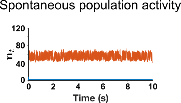
Figure S7: Spontaneous population activity simulated by the neuLVM before learning. Population activity of one excitatory population (the blue trace) quickly dies out. No visible metastable dynamics.

Table S2: Values of parameters used in simulations. Boldface is used to indicate fitted parameters.

	Name	Description	Value
			Example Section 5.1 Single excit. population	Example Section 5.2 Excitat. (inhib.) populations
	$\Delta t$	time step	1 ms	0.2 ms
	$N$	number of neurons	600	400 (200)
$\Theta$	$J$	connectivity	60.32 mV	9.984 mV (-19.968 mV)*
	$\vartheta$	firing threshold	49.7 mV	3.7 mV (3.7 mV)
	$U_{\mathrm{r}}$	resting potential	26 mV	14.4 mV (14.4 mV)
	$\tau_{\mathrm{mem}}$	membrane time constant	100 ms	20 ms (20 ms)
	$t_{\mathrm{ref}}$	absolute refractory period	0 ms	4 ms (4 ms)
$\epsilon$	$\tau_{\mathrm{syn}}$	synaptic time constant	4 ms	3 ms (6 ms)
	$\Delta$	synaptic delay	10 ms	0 ms (0 ms)

* i.e. for all population $\alpha$, $J^{\alpha\beta}=9.984$ mV if $\beta$ is an excitatory population and $J^{\alpha\beta}=-19.968$ mV if $\beta$ is the inhibitory population.

Table S3: Performance summary (ii) when fitting neuLVMs to the single-population example (Section 5.2, Figure 2C) with $m$-cluster states. For each ground truth $J$, $10$ different datasets were generated and tested. ($6$ observed neurons.)

$J$	59	60	61	62	63	64	65
$\widehat{J}$ (mean)	58.18	60.46	61.20	62.05	62.39	63.58	63.66
$\widehat{J}$ (std)	0.50	0.71	0.93	0.46	1.11	1.59	1.85
Pearson $r$	0.81 ($p=2.8\mathrm{e}{-17}$)

Table S4: Performance summary (i) when fitting neuLVMs to the single-population example (Section 5.2, Figure 2F) with a transition from a metastable 4-cluster state to a 3-cluster state. For each ground truth $J$, $10$ different datasets were generated and tested. ($J=60.32$ mV.)

# observed neurons	1	2	5	10	599
$\widehat{J}$ (mean)	60.37	60.14	59.33	59.81	59.10
$\widehat{J}$ (std)	2.43	1.48	0.91	1.25	1.26

Table S5: Hyper-parameters used when fitting neuLVM.

Name	Value
	Example Section 5.1 Single excit. population	Example Section 5.2 Excitat. (inhib.) populations
$\mathrm{lr}_{\mathrm{E}}$	$1\mathrm{e}{-3}$	$1\mathrm{e}{-3}$
$\mathrm{maxiter}_{\mathrm{E}}$	200	200
$\mathrm{itertol}_{\mathrm{E}}$	3	3
$\mathrm{lr}_{\mathrm{M}}$	$1\mathrm{e}{-8}$ *	$1\mathrm{e}{-8}$*
$\mathrm{maxiter}_{\mathrm{M}}$	200	200
$\mathrm{ftol}_{\mathrm{M}}$	$2\mathrm{e}{-9}$*	$2\mathrm{e}{-9}$*
$\mathrm{gtol}_{\mathrm{M}}$	$1\mathrm{e}{-5}$*	$1\mathrm{e}{-5}$*

* Values are default as in scipy.optimize.minimize(method=‘L-BFGS-B’).

Table S6: Within-population heterogeneity introduced in the ground truth winner-take-all (WTA) network (in the additional experiment of Appendix F).

ground truth within-population heterogeneity	$\mu$	$\sigma$ (normal distribution)
$J^{\textrm{e}^{1}}J^{\textrm{e}^{2}},J^{\textrm{i}}$	9.98 / 9.98 / 19.97	2.00 / 2.00 / 2.00
$\vartheta$	3.70	0.07
$U_{\mathrm{r}}$	14.40	0.29
$\tau_{\mathrm{mem}}$	20.00	0.40

Appendix G Checklist

1. For all authors…

   1. Do the main claims made in the abstract and introduction accurately reflect the paper’s contributions and scope? [Yes]

   2. Did you describe the limitations of your work? [Yes]

   3. Did you discuss any potential negative societal impacts of your work? [N/A]

   4. Have you read the ethics review guidelines and ensured that your paper conforms to them? [Yes]

2. If you are including theoretical results…

   1. Did you state the full set of assumptions of all theoretical results? [Yes]

   2. Did you include complete proofs of all theoretical results? [Yes]

3. If you ran experiments…

   1. Did you include the code, data, and instructions needed to reproduce the main experimental results (either in the supplemental material or as a URL)? [Yes] Code URL available upon acceptance or upon request.

   2. Did you specify all the training details (e.g., data splits, hyperparameters, how they were chosen)? [Yes]

   3. Did you report error bars (e.g., with respect to the random seed after running experiments multiple times)? [Yes]

   4. Did you include the total amount of computing and the type of resources used (e.g., type of GPUs, internal cluster, or cloud provider)? [N/A]

4. If you are using existing assets (e.g., code, data, models) or curating/releasing new assets…

   1. If your work uses existing assets, did you cite the creators? [Yes]

   2. Did you mention the license of the assets? [N/A]

   3. Did you include any new assets either in the supplemental material or as a URL? [N/A]

   4. Did you discuss whether and how consent was obtained from people whose data you’re using/curating? [N/A]

   5. Did you discuss whether the data you are using/curating contains personally identifiable information or offensive content? [N/A]

5. If you used crowdsourcing or conducted research with human subjects…

   1. Did you include the full text of instructions given to participants and screenshots, if applicable? [N/A]

   2. Did you describe any potential participant risks, with links to Institutional Review Board (IRB) approvals, if applicable? [N/A]

   3. Did you include the estimated hourly wage paid to participants and the total amount spent on participant compensation? [N/A]

unsrtnat mybib

References

- Steinmetz et al. [2018] Nicholas A Steinmetz, Christof Koch, Kenneth D Harris, and Matteo Carandini. Challenges and opportunities for large-scale electrophysiology with neuropixels probes. Current Opinion Neurobiology, 50:92–100, 2018.
- Gao and Ganguli [2015] Peiran Gao and Surya Ganguli. On simplicity and complexity in the brave new world of large-scale neuroscience. Current Opinion in Neurobiololy, 32:148–155, 2015.
- Pillow and Latham [2008] Jonathan W Pillow and Peter Latham. Neural characterization in partially observed populations of spiking neurons. Advances in Neural Information Processing Systems, 20:1161–1168, 2008.
- Brea et al. [2011] Johanni Brea, Walter Senn, and Jean-Pascal Pfister. Sequence learning with hidden units in spiking neural networks. Advances in Neural Information Processing Systems, 24:1422–1430, 2011.
- Rezende et al. [2011] Danilo Rezende, Daan Wierstra, and Wulfram Gerstner. Variational learning for recurrent spiking networks. Advances in Neural Information Processing Systems, 24:136–144, 2011.
- Bellec et al. [2021] Guillaume Bellec, Shuqi Wang, Alireza Modirshanechi, Johanni Brea, and Wulfram Gerstner. Fitting summary statistics of neural data with a differentiable spiking network simulator. Advances in Neural Information Processing Systems, 34:18552–18563, 2021.
- Gerstner [1995] Wulfram Gerstner. Time structure of the activity in neural network models. Physical Review E, 51(1):738, 1995.
- Brunel and Hakim [1999] Nicolas Brunel and Vincent Hakim. Fast global oscillations in networks of integrate-and-fire neurons with low firing rates. Neural Computation, 11(7):1621–1671, 1999.
- Gerstner [2000] Wulfram Gerstner. Population dynamics of spiking neurons: fast transients, asynchronous states, and locking. Neural Compututation, 12(1):43–89, 2000.
- Gerstner et al. [2014] Wulfram Gerstner, Werner M Kistler, Richard Naud, and Liam Paninski. Neuronal dynamics: From single neurons to networks and models of cognition. Cambridge University Press, 2014.
- Schwalger et al. [2017] Tilo Schwalger, Moritz Deger, and Wulfram Gerstner. Towards a theory of cortical columns: From spiking neurons to interacting neural populations of finite size. PLoS Computational Biology, 13(4):e1005507, 2017.
- Schwalger and Chizhov [2019] Tilo Schwalger and Anton V Chizhov. Mind the last spike—firing rate models for mesoscopic populations of spiking neurons. Current Opinion in Neurobiology, 58:155–166, 2019.
- Schmutz et al. [2021] Valentin Schmutz, Eva Löcherbach, and Tilo Schwalger. On a finite-size neuronal population equation. arXiv preprint arXiv:2106.14721, 2021.
- Lefort et al. [2009] Sandrine Lefort, Christian Tomm, J-C Floyd Sarria, and Carl CH Petersen. The excitatory neuronal network of the c2 barrel column in mouse primary somatosensory cortex. Neuron, 61(2):301–316, 2009.
- Potjans and Diesmann [2014] Tobias C Potjans and Markus Diesmann. The cell-type specific cortical microcircuit: relating structure and activity in a full-scale spiking network model. Cerebral Cortex, 24(3):785–806, 2014.
- Yoshimura et al. [2005] Yumiko Yoshimura, Jami LM Dantzker, and Edward M Callaway. Excitatory cortical neurons form fine-scale functional networks. Nature, 433(7028):868–873, 2005.
- Song et al. [2005] Sen Song, Per Jesper Sjöström, Markus Reigl, Sacha Nelson, and Dmitri B Chklovskii. Highly nonrandom features of synaptic connectivity in local cortical circuits. PLoS Biology, 3(3):e68, 2005.
- Clopath et al. [2010] Claudia Clopath, Lars Büsing, Eleni Vasilaki, and Wulfram Gerstner. Connectivity reflects coding: a model of voltage-based STDP with homeostasis. Nature Neuroscience, 13(3):344–352, 2010.
- Perin et al. [2011] Rodrigo Perin, Thomas K Berger, and Henry Markram. A synaptic organizing principle for cortical neuronal groups. Proceedings of the National Academy of Sciences, 108(13):5419–5424, 2011.
- Ko et al. [2011] Ho Ko, Sonja B Hofer, Bruno Pichler, Katherine A Buchanan, P Jesper Sjöström, and Thomas D Mrsic-Flogel. Functional specificity of local synaptic connections in neocortical networks. Nature, 473(7345):87–91, 2011.
- Litwin-Kumar and Doiron [2012] Ashok Litwin-Kumar and Brent Doiron. Slow dynamics and high variability in balanced cortical networks with clustered connections. Nature Neuroscience, 15(11):1498–1505, 2012.
- Shadlen and Newsome [1994] Michael N Shadlen and William T Newsome. Noise, neural codes and cortical organization. Current Opinion in Neurobiology, 4(4):569–579, 1994.
- Shadlen and Newsome [1998] Michael N Shadlen and William T Newsome. The variable discharge of cortical neurons: implications for connectivity, computation, and information coding. Journal of Neuroscience, 18(10):3870–3896, 1998.
- Vyas et al. [2020] Saurabh Vyas, Matthew D Golub, David Sussillo, and Krishna V Shenoy. Computation through neural population dynamics. Annual Review of Neuroscience, 43:249–275, 2020.
- Miller [2016] Paul Miller. Itinerancy between attractor states in neural systems. Current Opinion in Neurobiology, 40:14–22, 2016.
- La Camera et al. [2019] Giancarlo La Camera, Alfredo Fontanini, and Luca Mazzucato. Cortical computations via metastable activity. Current Opinion in Neurobiology, 58:37–45, 2019.
- Brinkman et al. [2022] Braden AW Brinkman, Han Yan, Arianna Maffei, Il Memming Park, Alfredo Fontanini, Jin Wang, and Giancarlo La Camera. Metastable dynamics of neural circuits and networks. Applied Physics Reviews, 9(1):011313, 2022.
- Latimer et al. [2015] Kenneth W Latimer, Jacob L Yates, Miriam LR Meister, Alexander C Huk, and Jonathan W Pillow. Single-trial spike trains in parietal cortex reveal discrete steps during decision-making. Science, 349(6244):184–187, 2015.
- Engel et al. [2016] Tatiana A Engel, Nicholas A Steinmetz, Marc A Gieselmann, Alexander Thiele, Tirin Moore, and Kwabena Boahen. Selective modulation of cortical state during spatial attention. Science, 354(6316):1140–1144, 2016.
- Mazzucato et al. [2019] Luca Mazzucato, Giancarlo La Camera, and Alfredo Fontanini. Expectation-induced modulation of metastable activity underlies faster coding of sensory stimuli. Nature Neuroscience, 22(5):787–796, 2019.
- Moreno-Bote et al. [2007] Rubén Moreno-Bote, John Rinzel, and Nava Rubin. Noise-induced alternations in an attractor network model of perceptual bistability. Journal of Neurophysiology, 98(3):1125–1139, 2007.
- Mazzucato et al. [2015] Luca Mazzucato, Alfredo Fontanini, and Giancarlo La Camera. Dynamics of multistable states during ongoing and evoked cortical activity. Journal of Neuroscience, 35(21):8214–8231, 2015.
- Macke et al. [2011] Jakob H Macke, Lars Buesing, John P Cunningham, Byron M Yu, Krishna V Shenoy, and Maneesh Sahani. Empirical models of spiking in neural populations. Advances in Neural Information Processing Systems, 24:1350–1358, 2011.
- Ackerson and Fu [1970] Guy Ackerson and K Fu. On state estimation in switching environments. IEEE Transactions on Automatic Control, 15(1):10–17, 1970.
- Ghahramani and Hinton [2000] Zoubin Ghahramani and Geoffrey E Hinton. Variational learning for switching state-space models. Neural Computation, 12(4):831–864, 2000.
- Barber [2006] David Barber. Expectation correction for smoothed inference in switching linear dynamical systems. Journal of Machine Learning Research, 7(11), 2006.
- Fox et al. [2008] Emily Fox, Erik Sudderth, Michael Jordan, and Alan Willsky. Nonparametric Bayesian learning of switching linear dynamical systems. Advances in Neural Information Processing Systems, 21:457–464, 2008.
- Petreska et al. [2011] Biljana Petreska, Byron M Yu, John P Cunningham, Gopal Santhanam, Stephen Ryu, Krishna V Shenoy, and Maneesh Sahani. Dynamical segmentation of single trials from population neural data. Advances in Neural Information Processing Systems, 24:756–764, 2011.
- Linderman et al. [2017] Scott Linderman, Matthew Johnson, Andrew Miller, Ryan Adams, David Blei, and Liam Paninski. Bayesian learning and inference in recurrent switching linear dynamical systems. In Artificial Intelligence and Statistics, pages 914–922. PMLR, 2017.
- Kulkarni and Paninski [2007] Jayant E Kulkarni and Liam Paninski. Common-input models for multiple neural spike-train data. Network: Computation in Neural Systems, 18(4):375–407, 2007.
- Lawhern et al. [2010] Vernon Lawhern, Wei Wu, Nicholas Hatsopoulos, and Liam Paninski. Population decoding of motor cortical activity using a generalized linear model with hidden states. Journal of Neuroscience Methods, 189(2):267–280, 2010.
- Vidne et al. [2012] Michael Vidne, Yashar Ahmadian, Jonathon Shlens, Jonathan W Pillow, Jayant Kulkarni, Alan M Litke, EJ Chichilnisky, Eero Simoncelli, and Liam Paninski. Modeling the impact of common noise inputs on the network activity of retinal ganglion cells. Journal of Computational Neuroscience, 33(1):97–121, 2012.
- Gao et al. [2016] Yuanjun Gao, Evan W Archer, Liam Paninski, and John P Cunningham. Linear dynamical neural population models through nonlinear embeddings. Advances in Neural Information Processing Systems, 29:163–171, 2016.
- Wu et al. [2017] Anqi Wu, Nicholas A Roy, Stephen Keeley, and Jonathan W Pillow. Gaussian process based nonlinear latent structure discovery in multivariate spike train data. Advances in Neural Information Processing Systems, 30:3496–3505, 2017.
- Pandarinath et al. [2018] Chethan Pandarinath, Daniel J O’Shea, Jasmine Collins, Rafal Jozefowicz, Sergey D Stavisky, Jonathan C Kao, Eric M Trautmann, Matthew T Kaufman, Stephen I Ryu, Leigh R Hochberg, et al. Inferring single-trial neural population dynamics using sequential auto-encoders. Nature Methods, 15(10):805–815, 2018.
- Duncker and Sahani [2018] Lea Duncker and Maneesh Sahani. Temporal alignment and latent gaussian process factor inference in population spike trains. Advances in neural information processing systems, 31:10445–10455, 2018.
- Duncker et al. [2019] Lea Duncker, Gergo Bohner, Julien Boussard, and Maneesh Sahani. Learning interpretable continuous-time models of latent stochastic dynamical systems. In International Conference on Machine Learning, pages 1726–1734. PMLR, 2019.
- Nassar et al. [2019] Josue Nassar, Scott Linderman, Monica Bugallo, and Il Memming Park. Tree-structured recurrent switching linear dynamical systems for multi-scale modeling. In International Conference on Learning Representations, 2019.
- Glaser et al. [2020] Joshua Glaser, Matthew Whiteway, John P Cunningham, Liam Paninski, and Scott Linderman. Recurrent switching dynamical systems models for multiple interacting neural populations. Advances in Neural Information Processing Systems, 33:14867–14878, 2020.
- Zoltowski et al. [2020] David Zoltowski, Jonathan Pillow, and Scott Linderman. A general recurrent state space framework for modeling neural dynamics during decision-making. In International Conference on Machine Learning, pages 11680–11691. PMLR, 2020.
- Rutten et al. [2020] Virginia Rutten, Alberto Bernacchia, Maneesh Sahani, and Guillaume Hennequin. Non-reversible Gaussian processes for identifying latent dynamical structure in neural data. Advances in Neural Information Processing Systems, pages 9622–9632, 2020.
- Keeley et al. [2020] Stephen Keeley, Mikio Aoi, Yiyi Yu, Spencer Smith, and Jonathan W Pillow. Identifying signal and noise structure in neural population activity with Gaussian process factor models. Advances in Neural Information Processing Systems, 33:13795–13805, 2020.
- Kim et al. [2021] Timothy D Kim, Thomas Z Luo, Jonathan W Pillow, and Carlos Brody. Inferring latent dynamics underlying neural population activity via neural differential equations. In International Conference on Machine Learning, pages 5551–5561. PMLR, 2021.
- René et al. [2020] Alexandre René, André Longtin, and Jakob H Macke. Inference of a mesoscopic population model from population spike trains. Neural Computation, 32(8):1448–1498, 2020.
- Paninski [2004] Liam Paninski. Maximum likelihood estimation of cascade point-process neural encoding models. Network: Computation in Neural Systems, 15(4):243–262, 2004.
- Truccolo et al. [2005] Wilson Truccolo, Uri T Eden, Matthew R Fellows, John P Donoghue, and Emery N Brown. A point process framework for relating neural spiking activity to spiking history, neural ensemble, and extrinsic covariate effects. Journal of Neurophysiology, 93(2):1074–1089, 2005.
- Pillow et al. [2008] Jonathan W Pillow, Jonathon Shlens, Liam Paninski, Alexander Sher, Alan M Litke, EJ Chichilnisky, and Eero P Simoncelli. Spatio-temporal correlations and visual signalling in a complete neuronal population. Nature, 454(7207):995–999, 2008.
- Zoltowski and Pillow [2018] David Zoltowski and Jonathan W Pillow. Scaling the Poisson GLM to massive neural datasets through polynomial approximations. Advances in Neural Information Processing Systems, 31:3517–3527, 2018.
- Lambert et al. [2018] Regis C Lambert, Christine Tuleau-Malot, Thomas Bessaih, Vincent Rivoirard, Yann Bouret, Nathalie Leresche, and Patricia Reynaud-Bouret. Reconstructing the functional connectivity of multiple spike trains using Hawkes models. Journal of Neuroscience Methods, 297:9–21, 2018.
- Kobayashi et al. [2019] Ryota Kobayashi, Shuhei Kurita, Anno Kurth, Katsunori Kitano, Kenji Mizuseki, Markus Diesmann, Barry J Richmond, and Shigeru Shinomoto. Reconstructing neuronal circuitry from parallel spike trains. Nature Communications, 10(1):1–13, 2019.
- Kistler et al. [1997] Werner M Kistler, Wulfram Gerstner, and J Leo van Hemmen. Reduction of the Hodgkin-Huxley equations to a single-variable threshold model. Neural Computation, 9(5):1015–1045, 1997.
- Jolivet et al. [2004] Renaud Jolivet, Timothy J Lewis, and Wulfram Gerstner. Generalized integrate-and-fire models of neuronal activity approximate spike trains of a detailed model to a high degree of accuracy. Journal of Neurophysiology, 92(2):959–976, 2004.
- Brette and Gerstner [2005] Romain Brette and Wulfram Gerstner. Adaptive exponential integrate-and-fire model as an effective description of neuronal activity. Journal of Neurophysiology, 94(5):3637–3642, 2005.
- Jolivet et al. [2006] Renaud Jolivet, Alexander Rauch, Hans-Rudolf Lüscher, and Wulfram Gerstner. Predicting spike timing of neocortical pyramidal neurons by simple threshold models. Journal of Computational Neuroscience, 21(1):35–49, 2006.
- Kobayashi et al. [2009] Ryota Kobayashi, Yasuhiro Tsubo, and Shigeru Shinomoto. Made-to-order spiking neuron model equipped with a multi-timescale adaptive threshold. Frontiers in Computational Neuroscience, 3:9, 2009.
- Pozzorini et al. [2015] Christian Pozzorini, Skander Mensi, Olivier Hagens, Richard Naud, Christof Koch, and Wulfram Gerstner. Automated high-throughput characterization of single neurons by means of simplified spiking models. PLoS Computational Biology, 11(6):e1004275, 2015.
- Teeter et al. [2018] Corinne Teeter, Ramakrishnan Iyer, Vilas Menon, Nathan Gouwens, David Feng, Jim Berg, Aaron Szafer, Nicholas Cain, Hongkui Zeng, Michael Hawrylycz, et al. Generalized leaky integrate-and-fire models classify multiple neuron types. Nature Communications, 9(1):1–15, 2018.
- Cox [1962] David Roxbee Cox. Renewal theory. Methuen, 1962.
- Wilson and Cowan [1972] Hugh R Wilson and Jack D Cowan. Excitatory and inhibitory interactions in localized populations of model neurons. Biophysical Journal, 12(1):1–24, 1972.
- De Masi et al. [2015] Anna De Masi, Antonio Galves, Eva Löcherbach, and Errico Presutti. Hydrodynamic limit for interacting neurons. Journal of Statistical Physics, 158(4):866–902, 2015.
- Fournier and Löcherbach [2016] Nicolas Fournier and Eva Löcherbach. On a toy model of interacting neurons. Annales de l’Institut Henri Poincaré, Probabilités et Statistiques, 52:1844–1876, 2016.
- Chevallier [2017a] Julien Chevallier. Mean-field limit of generalized Hawkes processes. Stochastic Processes and their Applications, 127(12):3870–3912, 2017a.
- Chevallier [2017b] Julien Chevallier. Fluctuations for mean-field interacting age-dependent Hawkes processes. Electronic Journal of Probability, 22, 2017b.
- Dumont et al. [2017] Grégory Dumont, Alexandre Payeur, and André Longtin. A stochastic-field description of finite-size spiking neural networks. PLoS Computational Biology, 13(8):e1005691, 2017.
- Schmutz et al. [2020] Valentin Schmutz, Wulfram Gerstner, and Tilo Schwalger. Mesoscopic population equations for spiking neural networks with synaptic short-term plasticity. The Journal of Mathematical Neuroscience, 10(1):1–32, 2020.
- Dempster et al. [1977] Arthur P Dempster, Nan M Laird, and Donald B Rubin. Maximum likelihood from incomplete data via the EM algorithm. Journal of the Royal Statistical Society: Series B (Methodological), 39(1):1–22, 1977.
- Smith and Brown [2003] Anne C Smith and Emery N Brown. Estimating a state-space model from point process observations. Neural Computation, 15(5):965–991, 2003.
- Yu et al. [2009] Byron M Yu, John P Cunningham, Gopal Santhanam, Stephen I Ryu, Krishna V Shenoy, and Maneesh Sahani. Gaussian-process factor analysis for low-dimensional single-trial analysis of neural population activity. Journal of Neurophysiology, 102(1):614–635, 2009.
- Ephraim and Merhav [2002] Yariv Ephraim and Neri Merhav. Hidden Markov processes. IEEE Transactions on Information Theory, 48(6):1518–1569, 2002.
- Allahverdyan and Galstyan [2011] Armen Allahverdyan and Aram Galstyan. Comparative analysis of Viterbi training and maximum likelihood estimation for HMMs. Advances in Neural Information Processing Systems, 24:1674–1682, 2011.
- Gerstner and van Hemmen [1993] Wulfram Gerstner and J Leo van Hemmen. Coherence and incoherence in a globally coupled ensemble of pulse-emitting units. Physical Review Letters, 71(3):312, 1993.
- Golomb and Rinzel [1994] David Golomb and John Rinzel. Clustering in globally coupled inhibitory neurons. Physica D: Nonlinear Phenomena, 72(3):259–282, 1994.
- Ernst et al. [1995] U Ernst, K Pawelzik, and T Geisel. Synchronization induced by temporal delays in pulse-coupled oscillators. Physical Review Letters, 74(9):1570, 1995.
- Wong and Wang [2006] Kong-Fatt Wong and Xiao-Jing Wang. A recurrent network mechanism of time integration in perceptual decisions. Journal of Neuroscience, 26(4):1314–1328, 2006.
- Lloyd [1982] Stuart Lloyd. Least squares quantization in PCM. IEEE Transactions on Information Theory, 28(2):129–137, 1982.
- van Rossum [2001] Mark CW van Rossum. A novel spike distance. Neural Computation, 13(4):751–763, 2001.
- Zhao and Park [2016] Yuan Zhao and Il Memming Park. Interpretable nonlinear dynamic modeling of neural trajectories. Advances in Neural Information Processing Systems, 29:3333–3341, 2016.
- Whiteway and Butts [2019] Matthew R Whiteway and Daniel A Butts. The quest for interpretable models of neural population activity. Current Opinion in Neurobiology, 58:86–93, 2019.
- Lueckmann et al. [2017] Jan-Matthis Lueckmann, Pedro J Goncalves, Giacomo Bassetto, Kaan Öcal, Marcel Nonnenmacher, and Jakob H Macke. Flexible statistical inference for mechanistic models of neural dynamics. Advances in Neural Information Processing Systems, 30:1289–1299, 2017.
- Penny et al. [2004] William D Penny, Klaas E Stephan, Andrea Mechelli, and Karl J Friston. Comparing dynamic causal models. Neuroimage, 22(3):1157–1172, 2004.
- Penny et al. [2010] Will D Penny, Klaas E Stephan, Jean Daunizeau, Maria J Rosa, Karl J Friston, Thomas M Schofield, and Alex P Leff. Comparing families of dynamic causal models. PLoS Computational Biology, 6(3):e1000709, 2010.
- Brodersen et al. [2011] Kay H Brodersen, Thomas M Schofield, Alexander P Leff, Cheng Soon Ong, Ekaterina I Lomakina, Joachim M Buhmann, and Klaas E Stephan. Generative embedding for model-based classification of fMRI data. PLoS Computational Biology, 7(6):e1002079, 2011.
Appendices of: