Exponential Random Graph Models for Dynamic Signed Networks: An Application to International Relations

Abstract

Substantive research in the Social Sciences regularly investigates signed networks, where edges between actors are either positive or negative. For instance, schoolchildren can be friends or rivals, just as countries can cooperate or fight each other. This research often builds on structural balance theory, one of the earliest and most prominent network theories, making signed networks one of the most frequently studied matters in social network analysis. While the theorization and description of signed networks have thus made significant progress, the inferential study of tie formation within them remains limited in the absence of appropriate statistical models. In this paper we fill this gap by proposing the Signed Exponential Random Graph Model (SERGM), extending the well-known Exponential Random Graph Model (ERGM) to networks where ties are not binary but negative or positive if a tie exists. Since most networks are dynamically evolving systems, we specify the model for both cross-sectional and dynamic networks. Based on structural hypotheses derived from structural balance theory, we formulate interpretable signed network statistics, capturing dynamics such as “the enemy of my enemy is my friend”. In our empirical application, we use the SERGM to analyze cooperation and conflict between countries within the international state system.

Keywords: Exponential Random Graph Models, Signed Networks, Structural Balance Theory, International Relations, Inferential Network Analysis

1 Introduction

In February 2022, Russia invaded Ukraine. This invasion shifted the relations that numerous European countries had with the belligerents. The EU member states, including previously Russia-aligned countries such as Hungary, sanctioned Russia and provide support to Ukraine. Belarus, a close ally of Russia, followed its partner into the conflict and was accordingly also sanctioned by the EU member states. And Turkey, a political and economic partner of both Ukraine and Russia, struggled to remain neutral in the conflict and thus sought to mediate between the belligerents. A meaningful geopolitical adjustment thus followed the Russian attack which demonstrates the importance of positive and negative ties in the international network of states, showing how pairwise cooperation and conflict between countries are interdependent.

Political scientists have studied this interplay of positive and negative ties between states since the early 1960s (Harary, 1961). In this context, international relations are conceived as signed networks, where the nodes are states and the edges are either positive, corresponding to bilateral cooperation, negative, expressing bilateral conflict, or non-existent. Most of this research builds on structural balance theory, which postulates that triads are balanced if they include an odd number of positive relations and unbalanced if that number is either even (“strong” structural balance; Heider, 1946; Cartwright and Harary, 1956) or exactly two (“weak” structural balance; Davis, 1967). Accordingly, International Relations scholars have studied whether specific triangular constellations correspond with these propositions (Harary, 1961; Healy and Stein, 1973; McDonald and Rosecrance, 1985; Doreian and Mrvar, 2015) and what implications structural balance has for community formation and system polarization (Hart, 1974; Lee et al., 1994). More recently, studies seek to test whether structural balance affects interstate conflict and cooperation in an inferential framework (Maoz et al., 2007; Lerner, 2016; Kinne and Maoz, 2022).

However, the study of signed networks is not restricted to International Relations. There are also applications to friendship and bullying between children (Huitsing et al., 2012, 2014), alliances and conflicts between tribal (Hage and Harary, 1984) or criminal groups (Nakamura et al., 2020), statements of support and opposition between politicians (Arinik et al., 2020; De Nooy and Kleinnijenhuis, 2013), and even to interactions within ecological networks (Saiz et al., 2017). In the setting of online social media and multiplayer games signed networks are also frequently studied (Leskovec et al., 2010; Bramson et al., 2021). Signed networks are thus a substantively important subject of study across and beyond the Social Sciences.

When working with signed networks, most techniques known from binary networks are not directly appropriate. A significant amount of work thus focuses on adapting blockmodels (Doreian and Mrvar, 2009; Jiang, 2015) as well as network statistics, such as centrality (Everett and Borgatti, 2014) and status (Bonacich and Lloyd, 2004), to signed networks. From an inferential perspective, the study of signed networks so far has mainly relied on logistic regression (Maoz et al., 2007; Lerner, 2016) or perceiving the observations as multivariate networks with multiple layers (Huitsing et al., 2012, 2014; Stadtfeld et al., 2020), where one level relates to the positive and another to the negative edges. While the former approach disregards endogenous dependence, the latter only allows for dependence between the separate observed layers of the network. Moreover, the multilayer approach does not adequately capture that most interactions in signed networks are either positive, negative, or non-existent. In other words, countries having negative and positive relations at the same time is unrealistic.

In the context of binary networks, Frank and Strauss (1986) proposed Exponential Random Graph Models (ERGMs) as a generative model for a network encompassing $n$ actors represented by the adjacency matrix ${\mathbf{y}}=({\mathbf{y}}_{ij})_{i,j=1,...,n}$, where $y_{ij}=1$ translates to an edge between actors $i$ and $j$ and ${y}_{ij}=0$ indicates that there is no edge. Henceforth, we use lowercase letters for variables when referring to the realized value of a random variable, i.e., the observed network $\mathbf{y}$, and capitalize the name to indicate that they are stochastic random variables, for instance, $\mathbf{Y}$. Within this framework, Wasserman and Pattison (1996) formulate a probability distribution over all possible $\mathbf{y}\in{\mathcal{Y}}$ by a canonical exponential family model:

$$\mathbb{P}_{\boldsymbol{\theta}}(\mathbf{Y}=\mathbf{y})=\frac{\exp\left\{\boldsymbol{\theta}^{\top}\mathbf{s}(\mathbf{y})\right\}}{\kappa(\boldsymbol{\theta})}~{}\forall~{}\mathbf{y}\in\mathcal{{Y}},$$ (1)

where $\mathcal{{Y}}$ is the set of all observable binary adjacency matrices among $n$ fixed actors, $s\text{ : }\mathcal{{Y}}\rightarrow\mathbb{R}^{q}$ is a function of sufficient statistics weighted by the coefficients $\theta\in\Theta\subseteq\mathbb{R}^{p}$, and $\kappa(\boldsymbol{\theta}):=\sum_{\tilde{\mathbf{y}}\in\mathcal{{Y}}}\exp\{\theta^{\top}\mathbf{s}(\tilde{\mathbf{y}})\}$ is a normalizing constant. Possible choices for the sufficient statistics $\mathbf{s}(\mathbf{{y}})$ of directed networks include the number of edges and triangles in the network (see Lusher et al., 2012 for a detailed overview of the model and other possible statistics). Depending on the specific sufficient statistics, ERGMs relax the often unrealistic conditional independence assumption inherent to most standard regression tools in dyadic contexts and allow general dependencies between the observed relations. Note that in many applications, auxiliary information $\mathbf{x}$ exogenous to the network is available, which can also be used in the sufficient statistics. For brevity of the notation, we, however, omit the dependence of $\mathbf{s}$ on $\mathbf{x}$. Due to this ability to flexibly specify dependence among relations, account for exogenous information, the desirable properties of exponential families, and versatile implementation in the $\mathtt{ergm}$ $\mathtt{R}$ package (Handcock et al., 2008; Hunter et al., 2008), the ERGM is a core inferential approach in the statistical analysis of networks.

In this article, we extend (1) to cover signed networks under general dependency assumptions and coin the term Signed Exponential Random Graph Model (SERGM) for the resulting model. The SERGM provides an inferential framework to test the predictions of, e.g., structural balance theory (Heider, 1946; Cartwright and Harary, 1956) without assuming that all observed relations are independent of one another. This characteristic is of vital importance given that balance theory explicitly posits that the sign of one relation depends on the state of other relations in the network. As the introductory examples suggest, interdependence-driven sign changes occur rapidly between states, necessitating the use of endogenous network statistics to adequately capture them. Along these lines, Lerner (2016, p. 75) notes that “tests of structural balance theory” should not rely on “models that assume independence of dyadic observations” and thereby flags the importance of developing an ERGM for signed networks. We answer this call by introducing, applying, and, via the $\mathtt{R}$ package $\mathtt{ergm.sign}$, providing statistical software in $\mathtt{R}$ (R Core Team, 2021) to implement the SERGM for static and dynamic networks, which is currently available at:

https://github.com/corneliusfritz/ergm.sign

We proceed as follows: In the consecutive section, we formally introduce the SERGM and a novel suite of sufficient statistics to capture network topologies specific to signed networks. In Section 3, we detail how to estimate the parameters of the SERGM and quantify the uncertainty of the estimates. Next, we apply the introduced model class to the interstate network of cooperation and conflict in Section 4. Finally, we conclude with a discussion of possible future extensions.

2 The Signed Exponential Random Graph Model

2.1 Model Formulation

First, we establish some notation to characterize signed networks. Assume that the signed adjacency matrix $\mathbf{y}=(y_{ij})_{i,j=1,...,n}$ was observed between $n$ actors. Contrasting the binary networks considered in (1), the entries of this signed adjacency matrix $y_{ij}$ are either “$+$”, “$-$”, or “0”, indicating a positive, negative, or no edge between actors $i$ and $j$. To ease notation, we limit ourselves to undirected networks without any self-loops, i.e., $\forall~{}i,j=1,...,n~{}y_{ij}=y_{ji}$ and $y_{ii}=$ “0” holds. Nevertheless, the proposed model naturally extends to directed settings. We denote the space encompassing all observable signed networks between $n$ actors by $\mathcal{Y}^{\pm}$ and specify a distribution over this space analogous to (1) in the following log-linear form:

$$\mathbb{P}_{\boldsymbol{\theta}}(\mathbf{{Y}}=\mathbf{{y}})=\frac{\exp\left\{\boldsymbol{\theta}^{\top}s(\mathbf{{y}})\right\}}{\kappa(\boldsymbol{\theta})}~{}\forall~{}\mathbf{y}\in\mathcal{Y}^{\pm}.$$ (2)

The function of sufficient statistics in (2) takes a signed network as its argument and determines the type of dependence between dyads in the network. A theoretically motivated suite of statistics one can incorporate as sufficient statistics follows in Section 2.2 but mirroring the term counting edges in binary networks, we can use the count of positive ties in signed network $\mathbf{y}$ via

$$EDGE^{+}(\mathbf{{y}})=\sum_{i<j}\mathbb{I}(y_{ij}=\text{``+''}),$$

where $\mathbb{I}(\cdot)$ is the indicator function. Along the same lines, one can define a statistic for the number of negative edges $EDGE^{-}(\mathbf{{y}})$ and use both statistics as intercepts in the model.

We can extend (2) to dynamic networks, which we denote by $\mathbf{Y}_{1},...,\mathbf{Y}_{T}$ for observations at $t=1,...,T$, by assuming a first-order Markov dependence structure to obtain

$$\mathbb{P}_{\boldsymbol{\theta}}(\mathbf{Y}_{t}=\mathbf{y}_{t}|\mathbf{Y}_{t-1}=\mathbf{y}_{t-1})=\frac{\exp\left\{\boldsymbol{\theta}^{\top}\mathbf{s}(\mathbf{y}_{t},\mathbf{y}_{t-1})\right\}}{\kappa(\boldsymbol{\theta},\mathbf{y}_{t-1})}~{}\forall~{}\mathbf{y}_{t}\in\mathcal{Y}^{\pm}.$$ (3)

The sufficient statistics encompassed in $\mathbf{s}(\mathbf{y}_{t},\mathbf{y}_{t-1})$ capture within-network or endogenous dependencies through statistics that only depend on $\mathbf{y}_{t}$ and between-network dependencies when incorporating $\mathbf{y}_{t-1}$. One instance for network statistics for between-network dependency is the stability statistic for positive edges

$$STABILITY^{+}(\mathbf{{y}}_{t},\mathbf{{y}}_{t-1})=\sum_{i<j}\mathbb{I}(y_{ij,t}=\text{``+''})\mathbb{I}(y_{ij,t-1}=\text{``+''}),$$

which can equivalently be defined for negative ties. Thus, we assume that the observed network is the outcome of a Markov chain with state space $\mathcal{Y}^{\pm}$ and transition probability (3). Of course, we may also include exogenous terms in (3), i.e., any pairwise- or actor-specific information external to $\mathbf{y_{t}}$.

For the interpretation of the estimates, techniques from binary ERGMs can be adapted. To derive a local tie-level interpretation, let $\theta_{q}$ with $q\in\{1,...,p\}$ denote the $q$th entry of $\theta$ corresponding to the $q$th sufficient statistic, $s_{q}(\mathbf{y}_{t},\mathbf{y}_{t-1})$. We further define ${\mathbf{y}_{t}}=(y_{ij,t})_{i,j=1,...,n}$ for $t=1,...,T$ and by $\mathbf{y}_{ij,t}^{+}$ denote the network $\mathbf{y}_{t}$ with the entry $y_{ij,t}$ fixed at “$+$”, $\mathbf{y}_{ij,t}^{-}$ and $\mathbf{y}_{ij,t}^{0}$ are established accordingly. Let $\mathbf{y}_{(-ij),t}$ refer to the network $\mathbf{y}_{t}$ excluding the entry $y_{ij,t}$. Due to the added complexity of signed networks, the distribution of $Y_{ij,t}$ conditional on $\mathbf{Y}_{(-ij),t}$ is a multinomial distribution where the event probability of entry “+” is:

$$\mathbb{P}_{\theta} (Y_{ij,t}=\text{``+''}|\mathbf{Y}_{(-ij),t}=\mathbf{y}_{(-ij),t-1},\mathbf{Y}_{t-1}=\mathbf{y}_{t-1})=\frac{\exp\left\{\boldsymbol{\theta}^{\top}\mathbf{s}(\mathbf{y}_{ij,t}^{+},\mathbf{y}_{t-1})\right\}}{\sum_{k\in\{+,-,0\}}\exp\left\{\boldsymbol{\theta}^{\top}\mathbf{s}(\mathbf{y}_{ij,t}^{k},\mathbf{y}_{t-1})\right\}}.$$ (4)

In the same manner, we can state the conditional probability of “$-$” and “0”. In accordance with change statistics from binary ERGMs, we subsequently define positive and negative change statistics through

$$\Delta_{ij,t}^{0\rightarrow+}(\mathbf{y}_{(-ij),t},\mathbf{y}_{t-1}) =\mathbf{s}(\mathbf{y}_{ij,t}^{+},\mathbf{y}_{t-1})-\mathbf{s}(\mathbf{y}_{ij,t}^{0},\mathbf{y}_{t-1})$$ (5)

$$\Delta_{ij,t}^{0\rightarrow-}(\mathbf{y}_{(-ij),t},\mathbf{y}_{t-1}) =\mathbf{s}(\mathbf{y}_{ij,t}^{-},\mathbf{y}_{t-1})-\mathbf{s}(\mathbf{y}_{ij,t}^{0},\mathbf{y}_{t-1}).$$

While the positive change statistic $\Delta_{ij,t}^{0\rightarrow+}(\mathbf{{y}}_{t},\mathbf{y}_{t-1})$ is the change in the sufficient statistics resulting from flipping the edge value of $y_{ij,t}$ from “0” to “+”, the negative change statistic $\Delta_{ij,t}^{0\rightarrow-}(\mathbf{{y}}_{t},\mathbf{y}_{t-1})$ relates to the change from “0” to “$-$”. By combining (4) and (5), we can obtain the relative log odds of $Y_{ij,t}$ to be “+” and “$-$” rather than “0”:

$$\log\left(\frac{\mathbb{P}_{\theta}(Y_{ij,t}=\text{``+''}|\mathbf{Y}_{(-ij),t}=\mathbf{y}_{(-ij),t},\mathbf{Y}_{t-1}=\mathbf{y}_{t-1})}{\mathbb{P}_{\theta}(Y_{ij,t}=\text{``0''}|\mathbf{Y}_{(-ij),t}=\mathbf{y}_{(-ij),t},\mathbf{Y}_{t-1}=\mathbf{y}_{t-1})}\right) =\theta^{\top}\Delta_{ij,t}^{0\rightarrow+}(\mathbf{y}_{(-ij),t},\mathbf{y}_{t-1})$$ (6)

$$\log\left(\frac{\mathbb{P}_{\theta}(Y_{ij,t}=\text{``$-$''}|\mathbf{Y}_{(-ij),t}=\mathbf{y}_{(-ij),t},\mathbf{Y}_{t-1}=\mathbf{y}_{t-1})}{\mathbb{P}_{\theta}(Y_{ij,t}=\text{``0''}|\mathbf{Y}_{(-ij),t}=\mathbf{y}_{(-ij),t},\mathbf{Y}_{t-1}=\mathbf{y}_{t-1})}\right) =\theta^{\top}\Delta_{ij,t}^{0\rightarrow-}(\mathbf{y}_{(-ij),t},\mathbf{y}_{t-1}).$$

This allows us to relate $\theta$ to the conditional distribution of $Y_{ij,t}$ given the rest of the network and derive two possible interpretations of the coefficients reminiscent of multinomial and logistic regression: the conditional log-odds of $Y_{ik,t}$ to be “$+$” rather than “$0$” are changed by the additive factor $\theta_{p}$, if the value of $y_{ij,t}$ changing from “0” to “$+$” raises the $p$th entry of $\Delta_{ij,t}^{0\rightarrow+}(\mathbf{y}_{(-ij),t},\mathbf{y}_{t-1})$ by one unit, while the other statistics remain unchanged. A similar interpretation holds for the negative change statistic.

Second, one can employ a global interpretation to understand the parameters on a network level. Then, $\theta_{q}>0$ indicates that higher values of $s_{q}(\mathbf{{y}}_{t},\mathbf{y}_{t-1})$ are expected under (2) than under a multinomial graph model, which we define as a simplistic network model where the value of each dyad is “+”, “$-$” and “0” with equal probability. In the opposing regime with $\theta_{q}<0$, we expect lower values than under this multinomial graph model.

2.2 From Structural Balance Theory to Sufficient Statistics

As discussed in the introduction, structural balance theory is a natural approach to signed networks. But so far, inferential work on it remains limited and uses, as we show below, suboptimal measures of its structural expectations. We thus shortly introduce the core logic of structural balance theory, discuss previous measures of it, and then derive sufficient statistics from it for inclusion in the SERGM. These statistics enable us to test the structural expectations formulated by structural balance theory in a principled manner within the framework introduced in Section 2.1.

Theory

The main implication of structural balance theory relates to the existence of triads between actors. Triads are the relations between three actors (Wasserman and Faust, 1994) and generally called balanced if they consist solely of positive ties (“the friend of my friend is my friend”) or one positive and two negative ties (“the enemy of my enemy is my friend”). According to structural balance theory, this type of triad should be observed more often than expected by chance in empirical signed networks. In contrast, triads that include a single negative tie are structurally imbalanced as the node participating in both positive relations has to cope with the friction of its two “friends” being opposed to each other. This actor should thus try to turn the negative tie into a positive tie to achieve a balanced constellation where all three actors share positive connections. But if this proves impossible, the actor will eventually have to choose a side, making one of its previously positive ties negative and resulting in structural balance. In triads where relations between all three actors are negative, the actors at least have incentives to make similar changes; these triads are thus also considered structurally imbalanced (Heider, 1946; Cartwright and Harary, 1956). In particular, two actors could reap benefits by developing a positive relationship, pooling their resources, and ganging up on the third node. However, later work views these triads without any positive ties as weakly balanced (Heider, 1958; Davis, 1967), as Davis (1967) notes that enemies of enemies being enemies indicates structural imbalance only if there are two subsets of nodes in the network. Triadic constellations with one negative relation are thus structurally imbalanced, should be empirically rare, and, where they exist, tend to turn into balanced states. Where only one negative tie exists, there is strong pressure to either eliminate it or create an additional one. And where there are three negative ties, actors at least have a clear incentive to turn one of them into a positive relation opportunistically, though their (im-)balance depends on the nature of the wider system (see also Easley and Kleinberg, 2010, ch. 5).

Testing Structural Balance via Lagged Statistics

Figure 1: Combining past and present ties can misrepresent structural (im-)balance: Triads observed at $t-1$ and $t$ are balanced (left side), combined triads are imbalanced (right side). Dashed lines indicate tie at $t-1$, solid ones at $t$. Dotted arrows show which ties from $t-1$ and $t$ contribute to the exogenous specification.

In interstate relations, this theory implies that two countries that are on friendly terms with the same other state should not wage war against each other. If three states all engage in conflict with each other, two of them may also find it beneficial to bury their hatchet, focus on their common enemy, and pool their resources against it. Along these lines, existing research asks whether two countries’ probability to cooperate or to fight is affected by them sharing common friends or foes (Maoz et al., 2007; Lerner, 2016). In particular, these authors investigate whether having shared allies or enemies at time $t-1$ affects the presence of positive and negative ties at $t$. The resulting “friend of my friend is my friend” statistic we can incorporate in the sufficient statistics of (3) is:

$$CF^{+}(\mathbf{y}_{t},\mathbf{y}_{t-1})=\sum_{i<j}\mathbb{I}(y_{ij,t}=\text{``+''})\left(\sum_{\begin{subarray}{c}h\neq i,h\neq j\end{subarray}}\mathbb{I}(y_{ih,t-1}=\text{``+''})\mathbb{I}(y_{jh,t-1}=\text{``+''})\right).$$ (7)

Similar delayed statistics can be defined for all other implications of the theory by treating the existence of common friends and foes as exogenous covariates. However, this approach comes with both theoretical and methodological problems. It is unclear whether actors wait a period (a calendar year in the case of Maoz et al., 2007 and Lerner, 2016) to adjust their relations towards structural balance and why they should do so as other applications of structural balance theory view these changes as instantaneous (see e.g. Kinne and Maoz, 2022). If the countries do not wait for a period, this approach can misrepresent the dynamics of signed networks as contradicting structural balance theory when they do not.

To illustrate this point, the right side of Figure 1 visualizes three structurally imbalanced constellations which Maoz et al. (2007) and Lerner (2016) uncover in the network of cooperation and conflict between states: (a) The friend of a friend being an enemy, (b) the enemy of an enemy being an enemy, and (c) the friend of an enemy being a friend. The left side of Figure 1 presents the triads at $t-1$ and $t$ these constellations are potentially made up of as ties are not observed simultaneously. The links of $i$ and $j$ to $h$ were observed at $t-1$ but those between $i$ and $j$ at $t$. The structurally imbalanced triads on the right side of Figure 1 thus consist of observations of the same triad made at two different points in time. Crucially, the left side of Figure 1 shows that both of these observations can themselves be structurally balanced. Exogenous measures of common friends and enemies can thus only capture the predictions of structural balance theory if (i) actors $i$ and $j$ wait a period until they change their tie sign due to their links to $h$ and (ii) their links to $h$ remain unchanged. Both of these conditions require strong assumptions regarding how actors behave within a network. In particular, structural balance theory implies that the edges between $i$, $j$, and $h$ are interdependent. But its exogenous operationalization assumes two of these edges as fixed while waiting to observe the third. An example shows that this is not just a theoretical issue, but mischaracterizes empirically observed relations between states: The US and Iran had common foes in 1978 but, in 1979, had become outright enemies themselves. The exogenous operationalization of structural balance regards this situation as unbalanced although it is an example of the scenario of Figure 1b.

Testing Structural Balance via Endogenous Statistics

Figure 2: Sufficient statistics for signed networks.

Therefore, endogenous network terms are necessary to capture the endogenous network dynamics postulated by structural balance theory. We next define endogenous statistics that mirror each constellation described by structural balance theory to test its predictions empirically. Building on the $k$-Edgewise-Shared Partner statistic developed to measure transitive closure in binary ERGMs (Hunter, 2007), we can define $k$-Edgewise-Shared Friends, $ESF_{k}(\mathbf{y})$, and $k-$Edgewise-Shared Enemies, $ESE_{k}(\mathbf{y}_{t})$, for signed networks. $ESF_{k}(\mathbf{y}_{t})$ counts the edges with $k$ shared friends and $ESE_{k}(\mathbf{y}_{t})$ those with $k$ shared enemies. We further differentiate between the state of the edge at the center of each triangular configuration and, e.g., write $ESF^{+}_{k}(\mathbf{y}_{t})$ and $ESF^{-}_{k}(\mathbf{y}_{t})$ as the version of the statistic where the value of $y_{ij}$ is “+” and “$-$”, respectively. Figure 2 illustrates the resulting four statistics.

For $k=2$ these statistics reduce to specific types of common triangle configurations (Holland and Leinhardt, 1972). However, as shown in Snijders et al. (2006), these types of statistics frequently lead to degenerate distributions where most of the probability mass is put on the empty or full graph (Handcock, 2003; Schweinberger, 2011). Moreover, the implied avalanche effect is particularly pronounced if the corresponding parameters are positive, as structural balance theory suggests. For binary ERGMs, it is thus standard to employ a statistic of the weighted sum of statistics in which the weights are proportional to the geometric sequence (Snijders et al., 2006; Hunter and Handcock, 2006). We follow this practice and define the geometrically weighted statistic for negative edgewise-shared enemies, as portrayed in Figure 2a, with a fixed decay parameter $\alpha$ as

$$GWESE^{+}(\mathbf{y}_{t},\alpha)=\exp\{\alpha\}\sum_{k=1}^{n-2}\left(1-\left(1-\exp\{-\alpha\}\right)\right)^{k}ESE^{+}_{k}(\mathbf{y}_{t}).$$ (8)

We establish the geometrically weighted variants of $ESE^{-}_{k}(\mathbf{y}_{t}),ESF^{+}_{k}(\mathbf{y}_{t}),$ and $ESF^{-}_{k}(\mathbf{y}_{t})$ accordingly. Each of these statistics reflects a specific type of triadic closure in signed networks as visualized in Figure 2. To interpret the coefficient $\theta_{GWESE^{+}}$ one can consider the logarithmic relative change in the probability according to (3) when increasing the number of common enemies of a befriended edge by one and keeping all other statistics constant. If the befriended actors already had $k$ prior common enemies before this change, this relative change is given by

$$\theta_{GWESE^{+}}\left(1-\left(1-\exp\{-\alpha\}\right)\right)^{k}.$$

Thus, if $\theta_{GWESE^{+}}>0$, each additional common enemy raises the probability to observe the signed network, although the increments become smaller for higher values of $k$. Hunter (2007) shows that these geometrical weighted statistics are equivalent to the alternating $k$-triangle statistics proposed by Snijders et al. (2006).

These triadic structures fully capture the logic of structural balance as they allow us to study the prevalence of triads where positive ties account for zero (Figure 2a) , one (Figure 2b), two (Figure 2c), and all three (Figure 2d) of the edges. According to this logic, we would expect the statistics $GWESE^{+}(\mathbf{y}_{t}$) and $GWESF^{+}(\mathbf{y}_{t}$) to be higher in empirical networks than expected by chance, but not $GWESE^{-}(\mathbf{y}_{t}$) and, particularly, $GWSF^{-}(\mathbf{y}_{t}$). If, on the other hand, the coefficients corresponding to $GWESE^{-}(\mathbf{y}_{t}$) or $GWESF^{-}(\mathbf{y}_{t}$) turn out to be positive in a network, this would offer empirical support for modifications of structural balance theory that also see the constellation in Figure 2a as balanced (Heider, 1958; Davis, 1967) or combine it with insights about, e.g., opportunism or reputation (Maoz et al., 2007). Mirroring the development of edge-wise shared enemy and friend statistics, it is also possible to compute dyad-wise statistics that do not require $i$ and $j$ to share a tie.

Other Sufficient Statistics

Besides these substantively informed statistics developed from structural balance theory, there are - as in the binary case - numerous other statistics one may incorporate into the model. Some of these are even necessary to isolate the effects of structural balance. In binary networks, closed triads where each node is connected to the others are more likely to form if the involved actors are highly active due to processes such as popularity. In the context of ERGMs, this phenomenon is captured by degree statistics counting the number of actors in the network with a specific number of edges. For signed networks, similar but more complicated processes may be at work and, to capture them, we define $DEG^{+}_{k}(\mathbf{y}_{t})$ and $DEG^{-}_{k}(\mathbf{y}_{t})$ as statistics that, respectively, count the number of actors in the signed network $\mathbf{y}_{t}$ with degree $k\in\{1,...,n-1\}$ for “+”- and “$-$”-signed links, respectively. Since the degree statistics are also prone to the degeneracy issues detailed above, we define geometrically-weighted equivalents for the positive and negative degrees. One can also incorporate exogenous statistics for the propensity to observe either a positive tie, similar to (7), via the following statistic:

$$EXO^{+}(\mathbf{y}_{t}) =\sum_{i<j}\mathbb{I}(y_{ij,t}=\text{``+''})x_{ij,t},$$

where $x_{ij,t}$ can be any pairwise scalar information. Similar statistics can be defined for negative, $EXO^{-}(\mathbf{y}_{t})$, and any , $EXO^{\pm}(\mathbf{y}_{t})$, tie. To test whether there is a tendency for homo- or heterophily based on actor attribute $x=(x_{1},...,x_{n})$ in the network, one may transform the nodal information to the pairwise level by setting $x_{ij,t}=|x_{i,t}-x_{j,t}|$ or $x_{ij,t}=\mathbb{I}(x_{i,t}=x_{j,t})$ for continuous and categorical attributes, respectively.

3 Estimation and Inference

To estimate $\theta$ for a fully specified set of sufficient statistics, we maximize the likelihood of (3) conditional on the initial network $\mathbf{y}_{0}$:

$$\mathcal{L}(\theta;\mathbf{y}_{1},...,\mathbf{y}_{T})= \prod_{t=1}^{T}\frac{\exp\left\{\boldsymbol{\theta}^{\top}\mathbf{s}(\mathbf{y}_{t},\mathbf{y}_{t-1})\right\}}{\kappa(\boldsymbol{\theta},\mathbf{y}_{t-1})}=\frac{\exp\left\{\boldsymbol{\theta}^{\top}\left(\sum_{t=1}^{T}\mathbf{s}(\mathbf{y}_{t},\mathbf{y}_{t-1})\right)\right\}}{\prod_{t=1}^{T}\kappa(\theta,\mathbf{y}_{t-1})}.$$ (9)

We can observe that this joint probability of the observed networks is still an exponential family, where the sufficient statistic is the sum of the individual statistics, the normalizing constant is composed of the product of the normalizing constants at each time point, and the canonical parameter is unchanged. Evaluating the normalizing constant in (9), on the other hand, necessitates the calculation of $T\cdot\left(3^{\frac{n(n-1)}{2}}\right)$ summands, making the direct evaluation of the likelihood prohibitive even for small networks. Fortunately, these difficulties are known from the analysis of binary networks and have been tackled in numerous articles (see, e.g., Strauss and Ikeda, 1990; Hummel et al., 2012; Snijders, 2002; Hunter and Handcock, 2006), which guide our estimation approach for the SERGM.

To circumvent the direct evaluation of (9), we can write the logarithmic likelihood ratio of $\theta$ and a fixed $\theta_{0}$ without a normalizing constant but an expected value

$$r(\theta,\theta_{0};\mathbf{y})= (\theta-\theta_{0})^{\top}\left(\sum_{t=1}^{T}\mathbf{s}(\mathbf{y}_{t},\mathbf{y}_{t-1})\right)$$ (10)

$$-\log\left(\mathbb{E}_{\theta_{0}}\left(\exp\left\{(\theta-\theta_{0})^{\top}\left(\sum_{t=1}^{T}\mathbf{s}(\mathbf{Y}_{t},\mathbf{y}_{t-1})\right)\right\}\right)\right).$$

We approximate the expectation in (10) by sampling networks over time, denoted by $\mathbf{Y}^{(m)}=(\mathbf{Y}_{1}^{(m)},...,\mathbf{Y}_{T}^{(m)})$ for the $m$th sample, whose dynamics are governed by (3) under $\theta_{0}$. Due to the Markov assumption, it suffices to specify only how to sample $\mathbf{Y}_{t}^{(m)}$ conditional on $\mathbf{y}_{t-1}$ for $t=1,...,T$ via Gibbs sampling. In particular, we generate a Markov chain with state space $\mathcal{Y}^{\pm}$ that, after a sufficient burn-in period, converges to samples from $\mathbf{Y}_{t}$ conditional on $\mathbf{y}_{t-1}$. Since we toggle one dyad in each iteration, the conditional probability distribution we sample from is the multinomial distributions stated in (4). In a setting where we sample $Y_{ij,t}$ conditional on $\mathbf{y}_{(-ij),t}$ and $\mathbf{y}_{t-1}$ with its present value given by $\tilde{y}_{ij,t}$, we can restate this conditional probability for “$+$” in terms of change statistics:

$$\mathbb{P}_{\theta}(Y_{ij,t}=\text{``+''}|\mathbf{Y}_{(-ij),t}=\mathbf{y}_{(-ij),t},\mathbf{Y}_{t-1}=\mathbf{y}_{t-1})=\frac{\exp\left\{\boldsymbol{\theta}^{\top}\Delta_{ij}^{\tilde{y}_{ij,t}\rightarrow+}(\mathbf{y}_{(-ij),t},\mathbf{y}_{t-1})\right\}}{\sum_{k\in\{+,-,0\}}\exp\left\{\boldsymbol{\theta}^{\top}\Delta_{ij}^{\tilde{y}_{ij,t}\rightarrow k}(\mathbf{y}_{(-ij),t},\mathbf{y}_{t-1})\right\}}.$$

This reformulation speeds up computation, since for most statistics the calculation of global statistics is computationally more demanding than the calculation of the change statistics defined in (5). Given $M$ sampled networks, we get

$$r(\theta,\theta_{0};\mathbf{y})\approx (\theta-\theta_{0})^{\top}\left(\sum_{t=1}^{T}\mathbf{s}(\mathbf{y}_{t},\mathbf{y}_{t-1})\right)$$ (11)

$$-\log\left(\frac{1}{M}\sum_{m=1}^{M}\exp\left\{(\theta-\theta_{0})^{\top}\left(\sum_{t=1}^{T}\mathbf{s}(\mathbf{y}_{t}^{(m)},\mathbf{y}_{t-1})\right)\right\}\right),$$

as an approximation of (10). However, according to standard theory of exponential families, the parameter $\theta$ maximizing (11) only exists if the sum of all observed sufficient statistics $\sum_{t=1}^{T}\mathbf{s}(\mathbf{y}_{t},\mathbf{y}_{t-1})$ under $\theta_{0}$ is inside the convex hull spanned by the sum of the sampled sufficient statistics (see Theorem 9.13 in Barndorff-Nielsen, 1978). Since this condition does not hold for arbitrary values of $\theta_{0}$, we modify the partial stepping algorithm under a log-normal assumption on the sufficient statistics introduced by Hummel et al. (2012) to dynamic signed networks for finding an adequate value for $\theta_{0}$ (details can be found in the Supplementary Material). We seed our algorithm with $\theta_{0}$ maximizing the pseudo-likelihood given by (4). To obtain estimates in the cross-sectional setting of (2), we can use the same procedure by setting $T=1$.

To quantify the sampling error of the estimates, we rely on the theory of exponential families stating that the Fisher information $\mathcal{I}(\theta)$ equals the variance of $\sum_{t=1}^{T}\mathbf{s}(\mathbf{Y}_{t},\mathbf{y}_{t-1})$ under the maximum likelihood estimate $\hat{\theta}$. We can estimate the Fisher information by again sampling networks $\mathbf{Y}^{(1)},...,\mathbf{Y}^{(M)}$ and calculating the empirical variance of
$\sum_{t=1}^{T}\mathbf{s}(\mathbf{y}_{t}^{(m)},\mathbf{y}_{t-1})$ for $m=1,...,M$. Due to the employed MCMC approximation, we follow standard practice of the $\mathtt{ergm}$ and $\mathtt{coda}$ packages (Handcock et al., 2008; Plummer et al., 2006) and estimate the MCMC standard error by the spectral density at frequency zero of the Markov chains of the statistics. For the final variance estimate, we sum up both types of errors. By extending the bridge sampler introduced in Hunter and Handcock (2006) to the SERGM for dynamic networks, we can also evaluate the AIC value of the model to carry out a model selection (see Supplementary Material).

4 Testing Structural Balance in International Cooperation and Conflict

4.1 Motivation

We now employ the SERGM to investigate relations of cooperation and conflict in the interstate network over the years 2000-2010. This application speaks directly to Maoz et al. (2007), Lerner (2016), and the many other studies on structural balance in international relations cited above. We focus on this period since it is the most current period for which we have comprehensive and reliable data and because 9/11 provided a structural break in international relations. We do not let $\theta$ vary over time here, but it would be reasonable to assume that 9/11 altered the dynamics of the interstate network (see Thurner et al., 2019). Hence $\theta$ likely changed from before to after 9/11 and we analyze only the 2000s. One example of this phenomenon is how states cooperate on their defense and security policies after 9/11. While alliances remain important, there is nowadays relatively little change in the alliance network from one year to another as “only a dozen new alliances have emerged since 9/11” (Kinne, 2020, p.730). Instead, a new type of formal commitment between states, defence cooperation agreements (DCA), have become widely used throughout the 1990s and 2000s (see Kinne, 2018, 2020). To ensure that we capture interstate cooperation in a meaningful manner for the period we are interested in, we depart from previous studies of structural balance in international relations and use DCAs instead of alliances to operationalize interstate cooperation. We do so for for several reasons.

First, as noted, the contemporary alliance network is basically static, experiencing little to no shifts over time. This is a challenge for estimation but, substantively, also severely limits the extent to which alliance relations could be affected by conflict between states. In contrast, DCAs are both initiated and terminated regularly (Kinne, 2018). Second, contemporary alliances are often multilateral and strongly institutionalized, meaning that if e.g. a new member joined NATO, it would result in the creation of several new alliance ties at once, but also that terminating these alliances, which have own secretariats, headquarters, and command structures, is challenging and thus empirically rare. Alliances hence do not clearly correspond to dyadic ties and have a life of their own which restricts tie deletion. In contrast, DCAs are bilateral and not as institutionalized, making them correspond much better to positive dyadic ties which can be formed but also removed (Kinne, 2018). Third, as opposed to alliances, DCAs are also signed by countries which have a policy of neutrality, thus reducing the risk that some ties are structural zeros, i.e. ineligible to be formed (Kinne, 2020). And fourth, most alliances only become active during armed conflict, stipulating wartime cooperation between their members (Leeds et al., 2002), but their goal is to deter enemies from instigating conflict in the first place. In other words, states’ formal commitment to cooperate, as demonstrated in an alliance, becomes realized only in a fraction of cases which are those where the alliance’s main goal, deterrence, has failed. In contrast, DCAs specify states’ commitment to and framework for peacetime, day-to-day defence cooperation regarding activities such as joint defence policies, military exercises, the co-development of military technology, and bilateral arms transfers (Kinne, 2018, 2020). DCAs therefore present a better dynamic measure of regular, bilateral defence cooperation between states for the 2000s than alliances do.

4.2 Model Specification

To measure cooperative, positively-signed interstate relations, we thus use the DCA data collected by Kinne (2020) and consider a tie as existent and positive if a pair of states shares at least one active DCA in year $t$. For conflictious, negatively-signed relations, we follow Maoz et al. (2007) and Lerner (2016) by using the Militarized Interstate Dispute (MID) Data provided by Palmer et al. (2021). MIDs are defined as “united historical cases of conflict in which the threat, display or use of military force short of war by one member state is explicitly directed towards the government, official representatives, official forces, property, or territory of another state” (Jones et al., 1996, p.163). We consider a tie to be existent and negative in year $t$ if a pair of states has at least one MID between them. We plot the resulting interstate network, consisting of positive DCA- and negative MID-ties, in the Supplementary Material.

To specificy a SERGM for modeling this evolving network, we first follow Maoz et al. (2007) and Lerner (2016) by including several exogenous covariates, namely $i$’s and $j$’s political difference, military capability ratio, the difference in wealth, and geographical distance. These variables’ sources are discussed in the Supplementary Material. Stemming from (3), we condition on the first year for the estimation and hence effectively model the network between 2001 and 2010.

Regarding endogenous statistics, the SERGM includes, most importantly, the four triadic terms developed above to capture the network’s tendency towards or against structural balance. Theoretically, we would expect the coefficients concerning $GWESE^{+}(\mathbf{y}_{t}$) and $GWESF^{+}(\mathbf{y}_{t})$ but not $GWESF^{-}(\mathbf{y}_{t})$ to have positive and statistically significant coefficients. For $GWESE^{-}(\mathbf{y}_{t})$, the expectation depends on whether we believe the state system to consist of two or of more groups (Davis, 1967). The latter appears more likely for the 2000s and we may thus expect to observe a positive coefficient. Furthermore, we include the positive and negative degree statistics, to capture highly active nodes’ propensity to (not) form more ties, and statistics that count the number of positive and negative edges as well as how many isolate nodes exist in each part of the network. Finally, stability terms are included to capture positive and negative ties remaining from the previous period. We term this specification Model 1 and present the results on the left side of Table 1.

We further compare Model 1 to a model specification where we replace the endogenous terms of structural balance, as depicted in Figure 2, with the exogenous versions used by Maoz et al. (2007) and Lerner (2016), stated in (7), where $i$’s and $j$’s ties with $h$ are observed not contemporaneously but in $t-1$. We denote the corresponding statistics by $CF^{+}(\mathbf{y}_{t},\mathbf{y}_{t-1})$ and $CF^{-}(\mathbf{y}_{t},\mathbf{y}_{t-1})$ to quantify the effect of common friends on positive and negative ties, while the number of common enemies are $CE^{+}(\mathbf{y}_{t},\mathbf{y}_{t-1})$ and $CE^{-}(\mathbf{y}_{t},\mathbf{y}_{t-1})$. Each of these exogenous measures corresponds to one of our triadic endogenous statistics, e.g. $CF^{+}(\mathbf{y}_{t},\mathbf{y}_{t-1})$ to $GWESF^{+}(\mathbf{y}_{t})$ and $CE^{-}(\mathbf{y}_{t},\mathbf{y}_{t-1})$ to $GWESE^{-}(\mathbf{y}_{t})$. Otherwise, the two models are identical as Model 2 includes the other endogenous statistics specified in Model 1. We can thus adjudicate whether operationalizing structural balance dynamics in an endogenous manner, implying that they occur instantaneously, is preferable over the exogenous specification where these dynamics occur with a one-period time delay.

4.3 Results

Table 1: Estimated coefficients and confidence intervals of the two model specifications detailed above. Dashes indicate the exclusion of covariates in a model specification. $\Delta$AIC indicates the difference between the AIC values of Model 1 and 2.

	Model 1			Model 2
	Coef.	CI		Coef.	CI
Edges $+$	-1.161	[-1.59,-0.732]		-0.689	[-1.203,-0.175]
Edges $-$	-1.754	[-2.142,-1.366]		-1.469	[-1.912,-1.026]
Isolates $+$	0.667	[-0.203,1.537]		0.462	[-0.422,1.346]
Isolates $-$	-1.188	[-2.319,-0.057]		-0.474	[-1.617,0.669]
Stability $+$	7.447	[7.331,7.563]		7.502	[7.379,7.625]
Stability $-$	5.531	[5.262,5.8]		5.594	[5.306,5.882]
Abs. Polity Diff. $+$	-0.022	[-0.032,-0.012]		-0.017	[-0.027,-0.007]
Abs. Polity Diff. $-$	0.004	[-0.016,0.024]		0.012	[-0.01,0.034]
CINC Ratio $+$	0.186	[0.117,0.255]		0.202	[0.129,0.275]
CINC Ratio $-$	-0.168	[-0.293,-0.043]		-0.14	[-0.279,-0.001]
Abs. GDP Diff. $+$	-0.521	[-0.57,-0.472]		-0.495	[-0.554,-0.436]
Abs. GDP Diff. $-$	-1.04	[-2.651,0.571]		-1.311	[-3.069,0.447]
Abs. Distance $\pm$	3.324	[0.515,6.133]		2.796	[-0.428,6.02]
$GWESE^{+}$ (Fig. 2a)	0.618	[0.308,0.928]		-
$GWESE^{-}$ (Fig. 2b)	0.515	[0.199,0.831]		-
$GWESF^{+}$ (Fig. 2c)	0.489	[0.415,0.563]		-
$GWESF^{-}$ (Fig. 2d)	0.319	[0.178,0.46]		-
$GWD^{+}$	-2.214	[-2.577,-1.851]		-2.625	[-3.015,-2.235]
$GWD^{-}$	-0.321	[-1.617,0.975]		-0.998	[-2.276,0.28]
$CF^{+}$	-			0.069	[0.051,0.087]
$CF^{-}$	-			0.077	[0.04,0.114]
$CE^{+}$	-			0.374	[-0.042,0.79]
$CE^{-}$	-			0.304	[-0.239,0.847]
$\Delta$AIC	0			599.894

Below, we interpret the results of the endogenous network terms and their exogenous equivalents. We discuss the coefficient estimates of the exogenous covariates in the Supplementary Material. As expected, both the $GWESF^{+}(\mathbf{y}_{t})$ and the $GWESE^{+}(\mathbf{y}_{t})$ terms exhibit positive and statistically significant coefficients, with neither confidence interval encompassing zero. These results align with structural balance theory in that both “the friend of my friend” and “the enemy of my enemy” are my friend. But we also find that the $GWESF^{-}(\mathbf{y}_{t})$ and $GWESE^{-}(\mathbf{y}_{t})$ coefficients are positive and statistically significant, albeit with smaller effects and confidence intervals closer to zero than in the case of the first two statistics. In the studied interstate network, there is thus also a tendency towards enemies of enemies being enemies. This echoes the point that triangles with three negative ties are imbalanced only in systems with two subsets (Davis, 1967), a condition that may have been present in the highly bipolar first half of the Cold War, but not more than a decade after its termination. This result is thus consistent with the verdict that, against early formulations of structural balance theory (Heider, 1946; Cartwright and Harary, 1956), “if two negative relations are given, balance can be obtained either when the third relationship is positive or when it is negative” (Heider, 1958, p.206). Observing that the effect of $GWESE^{-}(\mathbf{y}_{t})$ is positive and statistically significant underlines the importance of overall network structure for the predictions of structural balance theory.

We also find that friends of friends have an increased probability of being enemies. In the international relations of the 2000s, what seems to hold is that both enemies of enemies and friends of friends are more likely to interact than if they did not share relations with a common third state. Friends of friends being more likely to fight than to have no relation at all suggests that shared relations may also indicate the “reachability” of one state to another within a system where some dyads, e.g., that between Lesotho and Belize, have a very low structural probability of ever being active (see, e.g. Quackenbush, 2006). Triadic closure, regardless of the sign, thus exists also in the network of cooperation and conflict between states. However, we observe that the tendency towards such closure is stronger for structurally balanced relations than for structurally imbalanced ones.

A comparison of the two model specifications shown in Table 1 allows us to ascertain whether specifying the triadic relationships endogenously affects substantive results and model performance. Here, it is visible that the AIC of the model with the endogenous statistics is lower than that with their exogenous versions. Specifying interdependent dynamics in the interstate network via endogenous covariates hence increases model performance compared to trying to capture them by including lagged, exogenous variables.

More strikingly, Table 1 shows that the substantive results of the corresponding endogenous and exogenous measures of structural balance dynamics differ significantly. Contrasting the results under the endogenous and exogenous model specification, the latter offers much more limited support for these notions. While the coefficient of $CF^{+}(\mathbf{y}_{t},\mathbf{y}_{t-1})$ is positive and statistically significant, its effect size is still very close to zero. The “friends of friends are friends”-effect is thus found to be substantively negligible in Model 2. In contrast, the coefficient of $CE^{+}(\mathbf{y}_{t},\mathbf{y}_{t-1})$ is positive and substantively larger, while its 95$\%$-confidence interval includes zero, indicating that the model cannot statistically distinguish it from zero as its estimation is very imprecise. The statistics $CF^{-}(\mathbf{y}_{t},\mathbf{y}_{t-1})$ and $CE^{-}(\mathbf{y}_{t},\mathbf{y}_{t-1})$ mirror their corresponding endogenous terms from Model 1 in that both exhibit positive coefficients but, again, the first is substantively much smaller and the second one very imprecisely estimated. On the whole, this comparison of an endogenous and an exogenous specification of the triadic configurations motivated by structural balance theory thus shows that Model 1 is preferable over Model 2. The model including endogenous terms thus not only provides better performance than that with their exogenous counterparts but these terms are also estimated to be more influential and more precisely.

4.4 Model Assessment

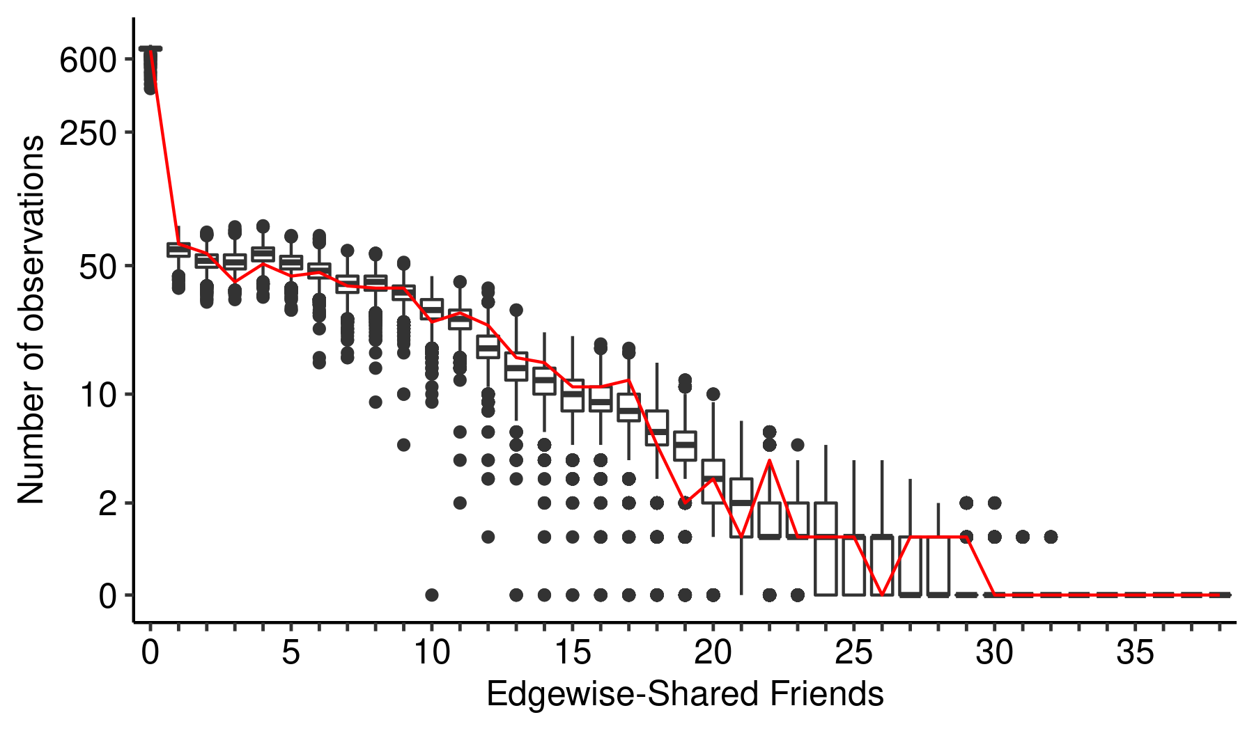
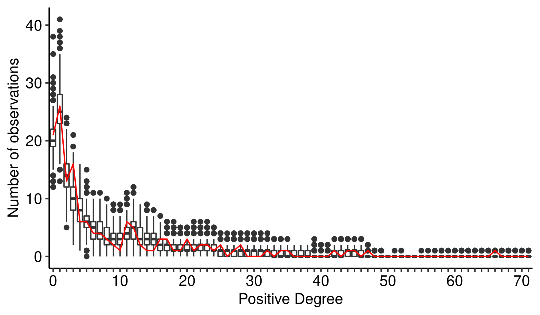
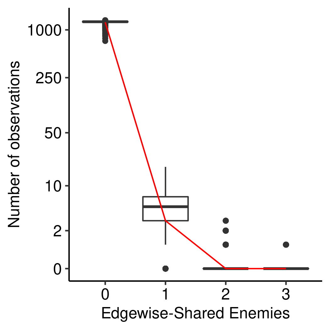
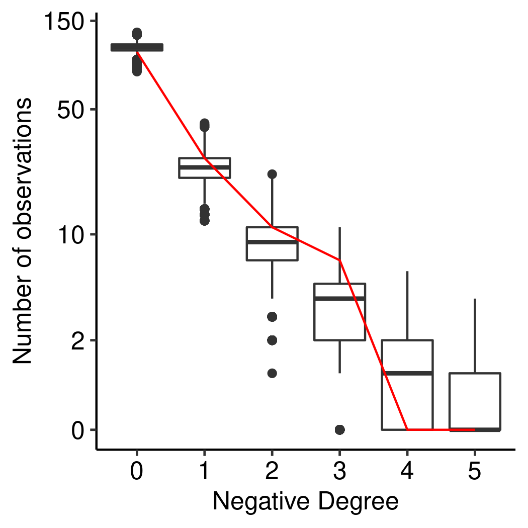
Figure 3: Goodness-of-fit assessment in year 2005.

To assess the fit of the estimated SERGM, we employ a graphical tool inspired by Hunter et al. (2008) to evaluate whether it can adequately represent topologies of the observed network not explicitly incorporated as sufficient statistics in (3). Therefore, we sample networks from (3), compute the statistics, summarize them, and then compare this summary to the statistics evaluated on the observed network. Heuristically, a model generating simulations that better reflect the observed values also has a better goodness-of-fit. To cover signed networks, we investigate the observed and simulated distributions of positive and negative degrees, and edgewise-shared enemies and friends in the interstate network.

We report the goodness-of-fit plots for Model 1 from Table 1 in Figure 3 for the year 2005. In each subplot, a series of box plots display the distribution of a given value of the statistic under consideration over the networks simulated from the model via the Gibbs Sampler detailed in Section 3. The red line indicates where the statistic is measured in the observed network and should thus, ideally, lie close to the median value of the simulated networks, i.e., the center of the box plots. In Figure 3, this is the case for all four statistics, indicating that Model 1 under the estimated parameters generalizes well to network topologies not explicitly incorporated in the sufficient statistics.

Together, the results presented here indicate that the SERGM is able to uncover structural balance dynamics in the interstate network and is preferable over approaches that seek to model signed interstate networks under conditional independence, but also that further substantial research on structural balance in international relations is neeeded. The Supplementary Material employs the SERGM to analyze a cross-sectional network, representing enmity and friendship among New Guinean Highland Tribes (Hage and Harary, 1984), and shows its applicability when there is no observable temporal dependence structure.

5 Discussion

We extended the core regression model for network data to dynamic and cross-sectional signed networks. Given the theoretical foundation of structural balance, we introduce novel endogenous statistics that offer better performance than operationalizing them by lagged covariates, as commonly done in previous research. Finally, we apply the method to recent data on militarized interstate disputes and defense cooperation agreements and provide a software implementation with the $\mathtt{R}$ package $\mathtt{ergm.sign}$.

From a substantive point of view, this research offers new insights on the empirical testing of structural balance theory and challenges earlier inferential studies on the topic. How one captures structural balance matters. We show that an approach relying on past observations of some ties within a triad to measure structural balance as an exogenous variable can mischaracterize triadic (im-)balance. We thus develop endogenous balance measures that can be used in the SERGM framework and show empirically that these endogenous measures result in different substantive results as well as increased model performance as compared to the exogenous ones. Most importantly, the exogenous measures do not affect tie formation consistent with structural balance theory, whereas when employing the endogenous ones, we find evidence in line with it. States are thus more likely to cooperate if they share common partners or are hostile to the same enemies. This indicates that there is structural balance in interstate cooperation and conflict, at least when studying the 2000s. Future work in International Relations should seek to build on this fundamental result to test whether it also holds for earlier periods, for instance the bipolar Cold War years, and how structural balance interacts with exogenous factors such as military capabilities. Beyond International Relations, the SERGM will also serve to advance research across all Social Sciences, allowing researchers to investigate tie formation in networks of friendship and enmity between school children, gangs, or social media accounts.

At the same time, we find that, generally, states appear more likely to interact, positively or negatively, when they share friends or enemies. Substantively, this result suggests that, additional to structural balance, something else is at play and may indicate that some state dyads are structurally very unlikely to ever be active, due to the countries’ distance, lack of economic development, and/or power projection capabilities, mirroring research on politically “relevant” or “active” dyads (see Quackenbush, 2006). But this implied variation in “reachability” between states also points to the fact that structural balance theory was developed on complete networks, where every possible ties is realized with either a negative or a positive sign, while empirical networks are usually incomplete (see Easley and Kleinberg, 2010, ch.5). It thus lends some support to Lerner’s (2016) argument that tests of structural balance theory should not examine states’ marginal probability to cooperate or fight, but instead their probability of cooperating or fighting conditional upon them interacting. However, following Lerner’s (2016, Sec. 4.2.1) argument on the use of ERGMs in conjunction with this conditional viewpoint, it becomes evident that (3) is consistent with it. Defining $\mathbf{Y}^{|\pm|}$ with $Y^{|\pm|}_{ij}=1\text{ if }Y_{ij}\neq$ “0” as the random adjacency matrix describing any type of interaction and $\mathcal{Y}$, be it positive or negative, one can derive the following conditional probability distribution

$$\mathbb{P}_{\boldsymbol{\theta}}(\mathbf{Y}_{t}=\mathbf{y}_{t}|\mathbf{Y}^{|\pm|}_{t}=\mathbf{y}^{|\pm|}_{t},\mathbf{Y}_{t-1}=\mathbf{y}_{t-1})=\frac{\exp\left\{\boldsymbol{\theta}^{\top}\mathbf{s}(\mathbf{y}_{t},\mathbf{y}_{t-1})\right\}}{\tilde{\kappa}(\boldsymbol{\theta},\mathbf{y}_{t-1},\mathbf{y}^{|\pm|}_{t})}~{}\forall~{}\mathbf{y}_{t}\in\mathcal{Y}^{\pm},$$ (12)

where $\tilde{\kappa}(\boldsymbol{\theta},\mathbf{y}_{t-1},\mathbf{y}^{|\pm|}_{t})=\sum_{\tilde{\mathbf{y}}\in\mathcal{Y}^{\pm}}\mathbb{I}(\mathbf{\tilde{y}}^{|\pm|}=\mathbf{y}^{|\pm|}_{t})\exp\left\{\boldsymbol{\theta}^{\top}\mathbf{s}(\tilde{\mathbf{y}},\mathbf{y}_{t-1})\right\}$. The conditional distribution (12) is thus a SERGM with support limited to networks where $\mathbf{y}^{|\pm|}_{t}$ is equal to the observed network and the coefficients of (12) are unchanged. Therefore, (3) implies (12).

Alternatively, some dyads’ lack of “reachability” may also indicate that dependency structures are not fully global, even in international relations where all actors know of each other. Major powers should generally be able to reach all other states in the system, thus also making their actions globally relevant, but smaller countries’ reach and relevance will be more locally limited. Since the more general framework of ERGMs in (1) relies on homogeneity assumptions implying that each endogenous mechanism has the same effect in the entire network, model (3) might assume dependence between relations where, in reality, there is none. One possible endeavor for future research would be adapting local dependence (Schweinberger and Handcock, 2015) to signed and dynamic networks. This approach assumes complex dependency solely within either observed or unobserved groups of the actors, solving the obstacle of “reachability” between some countries in the network. At the same time, other extensions of ERGMs, be it actor-specific random effects or curved ERGMs where $\alpha$ in (8) is estimated from the data, are also feasible under (2) and (3).

References

- Arinik et al. (2020) Arinik, N., R. Figueiredo, and V. Labatut (2020). Multiple partitioning of multiplex signed networks: Application to european parliament votes. Social Networks 60, 83–102.
- Barndorff-Nielsen (1978) Barndorff-Nielsen, O. (1978). Information and exponential families in statistical theory. New York: Wiley.
- Bonacich and Lloyd (2004) Bonacich, P. and P. Lloyd (2004). Calculating status with negative relations. Social Networks 26(4), 331–338.
- Bramson et al. (2021) Bramson, A., K. Hoefman, K. Schoors, and J. Ryckebusch (2021). Diplomatic relations in a virtual world. Political Analysis, 1–22.
- Cartwright and Harary (1956) Cartwright, D. and F. Harary (1956). Structural balance: A generalization of heider’s theory. Psychological Review 63(5), 277–293.
- Davis (1967) Davis, J. A. (1967). Clustering and structural balance in graphs. Human Relations 20(2), 181–187.
- De Nooy and Kleinnijenhuis (2013) De Nooy, W. and J. Kleinnijenhuis (2013). Polarization in the media during an election campaign: A dynamic network model predicting support and attack among political actors. Political Communication 30(1), 117–138.
- Doreian and Mrvar (2009) Doreian, P. and A. Mrvar (2009). Partitioning signed social networks. Social Networks 31(1), 1–11.
- Doreian and Mrvar (2015) Doreian, P. and A. Mrvar (2015). Structural balance and signed international relations. Journal of Social Structure 16(1), 1–49.
- Easley and Kleinberg (2010) Easley, D. and J. Kleinberg (2010). Networks, crowds, and markets: Reasoning about a highly connected world. Cambridge University Press.
- Everett and Borgatti (2014) Everett, M. G. and S. P. Borgatti (2014). Networks containing negative ties. Social Networks 38(1), 111–120.
- Frank and Strauss (1986) Frank, O. and D. Strauss (1986). Markov graphs. Journal of the American Statistical Association 81(395), 832–842.
- Hage and Harary (1984) Hage, P. and F. Harary (1984). Structural Models in Anthropology. Cambridge: Cambridge University Press.
- Handcock (2003) Handcock, M. (2003). Assessing degeneracy in statistical models of social networks. Technical report, University of Washington.
- Handcock et al. (2008) Handcock, M. S., D. R. Hunter, C. T. Butts, S. M. Goodreau, and M. Morris (2008). statnet: Software tools for the representation, visualization, analysis and simulation of network data. Journal of Statistical Software 24(1), 1–11.
- Harary (1961) Harary, F. (1961). A structural analysis of the situation in the middle east in 1956. Journal of Conflict Resolution 5(2), 167–178.
- Hart (1974) Hart, J. (1974). Symmetry and polarization in the european international system, 1870 - 1879: A methodological study. Journal of Peace Research 11(3), 229–244.
- Healy and Stein (1973) Healy, B. and A. Stein (1973). The balance of power in international history: Theory and reality. Journal of Conflict Resolution 17(1), 33–61.
- Heider (1946) Heider, F. (1946). Attitudes and cognitive organization. Journal of Psychology 21(1), 107–112.
- Heider (1958) Heider, F. (1958). The psychology of interpersonal relations. New York: Wiley.
- Holland and Leinhardt (1972) Holland, P. W. and S. Leinhardt (1972). Some evidence on the transitivity of positive interpersonal sentiment. American Journal of Sociology 77(6), 1205–1209.
- Huitsing et al. (2014) Huitsing, G., T. A. B. Snijders, M. A. J. Van Duijn, and R. Veenstra (2014). Victims, bullies, and their defenders: A longitudinal study of the coevolution of positive and negative networks. Development and Psychopathology 26(3), 645–659.
- Huitsing et al. (2012) Huitsing, G., M. A. van Duijn, T. A. Snijders, P. Wang, M. Sainio, C. Salmivalli, and R. Veenstra (2012). Univariate and multivariate models of positive and negative networks: Liking, disliking, and bully–victim relationships. Social Networks 34(4), 645–657.
- Hummel et al. (2012) Hummel, R. M., D. R. Hunter, and M. S. Handcock (2012). Improving simulation-based algorithms for fitting ERGMs. Journal of Computational and Graphical Statistics 21(4), 920–939.
- Hunter (2007) Hunter, D. R. (2007). Curved exponential family models for social networks. Social Networks 29(2), 216–230.
- Hunter et al. (2008) Hunter, D. R., S. M. Goodreau, and M. S. Handcock (2008). Goodness of fit of social network models. Journal of the American Statistical Association 103(481), 248–258.
- Hunter and Handcock (2006) Hunter, D. R. and M. S. Handcock (2006). Inference in curved exponential family models for networks. Journal of Computational and Graphical Statistics 15(3), 565–583.
- Hunter et al. (2008) Hunter, D. R., M. S. Handcock, C. T. Butts, S. M. Goodreau, and M. Morris (2008). ergm: A package to fit, simulate and diagnose exponential-family models for networks. Journal of Statistical Software 24(3), 1–29.
- Jiang (2015) Jiang, J. Q. (2015). Stochastic block model and exploratory analysis in signed networks. Physical Review E 91(6), 062805.
- Jones et al. (1996) Jones, D. M., S. A. Bremer, and J. D. Singer (1996). Militarized interstate disputes, 1816–1992: Rationale, coding rules, and empirical patterns. Conflict Management and Peace Science 15(2), 163–213.
- Kinne (2018) Kinne, B. J. (2018). Defense cooperation agreements and the emergence of a global security network. International Organization 72(4), 799–837.
- Kinne (2020) Kinne, B. J. (2020). The defense cooperation agreement dataset (dcad). Journal of Conflict Resolution 64(4), 729–755.
- Kinne and Maoz (2022) Kinne, B. J. and Z. Maoz (2022). Local politics, global consequences: How structural imbalance in domestic political networks affects international relations. Journal of Politics (OnlineFirst).
- Lee et al. (1994) Lee, S. C., R. G. Muncaster, and D. A. Zinnes (1994). The friend of my enemy is my enemy: Modeling triadic internation relationships. Synthese 100(3), 333–358.
- Leeds et al. (2002) Leeds, B., J. Ritter, S. Mitchell, and A. Long (2002). Alliance treaty obligations and provisions, 1815-1944. International Interactions 28(3), 237–260.
- Lerner (2016) Lerner, J. (2016). Structural balance in signed networks: Separating the probability to interact from the tendency to fight. Social Networks 45, 66–77.
- Leskovec et al. (2010) Leskovec, J., D. Huttenlocher, and J. Kleinberg (2010). Signed networks in social media. In Proceedings of the 28th international conference on Human factors in computing systems, pp. 1361–1370.
- Lusher et al. (2012) Lusher, D., J. Koskinen, and G. Robins (2012). Exponential random graph models for social networks. Cambridge: Cambridge University Press.
- Maoz et al. (2007) Maoz, Z., L. G. Terris, R. D. Kuperman, and I. Talmud (2007). What is the enemy of my enemy? causes and consequences of imbalanced international relations, 1816–2001. Journal of Politics 69(1), 100–115.
- McDonald and Rosecrance (1985) McDonald, H. B. and R. Rosecrance (1985). Alliance and structural balance in the international system: A reinterpretation. Journal of Conflict Resolution 29(1), 57–82.
- Nakamura et al. (2020) Nakamura, K., G. Tita, and D. Krackhardt (2020). Violence in the “balance”: A structural analysis of how rivals, allies, and third-parties shape inter-gang violence. Global Crime 21(1), 3–27.
- Palmer et al. (2021) Palmer, G., R. W. McManus, V. D’Orazio, M. R. Kenwick, M. Karstens, C. Bloch, N. Dietrich, K. Kahn, K. Ritter, and M. J. Soules (2021). The mid5 dataset, 2011–2014: Procedures, coding rules, and description. Conflict Management and Peace Science 39(4), 470–482.
- Plummer et al. (2006) Plummer, M., N. Best, K. Cowles, and K. Vines (2006). Coda: Convergence diagnosis and output analysis for mcmc. R News 6(1), 7–11.
- Quackenbush (2006) Quackenbush, S. L. (2006). Identifying opportunity for conflict: Politically active dyads. Conflict Management and Peace Science 23(1), 37–51.
- R Core Team (2021) R Core Team (2021). R: A language and environment for statistical computing. Vienna, Austria: R Foundation for Statistical Computing.
- Saiz et al. (2017) Saiz, H., J. Gómez-Gardeñes, P. Nuche, A. Girón, Y. Pueyo, and C. L. Alados (2017). Evidence of structural balance in spatial ecological networks. Ecography 40(6), 733–741.
- Schweinberger (2011) Schweinberger, M. (2011). Instability, sensitivity, and degeneracy of discrete exponential families. Journal of the American Statistical Association 106(496), 1361–1370.
- Schweinberger and Handcock (2015) Schweinberger, M. and M. S. Handcock (2015). Local dependence in random graph models: Characterization, properties and statistical inference. Journal of the Royal Statistical Society: Series B (Statistical Methodology) 77(3), 647–676.
- Snijders (2002) Snijders, T. A. B. (2002). Markov Chain Monte Carlo estimation of exponential random graph models. Journal of Social Structure.
- Snijders et al. (2006) Snijders, T. A. B., P. E. Pattison, G. L. Robins, and M. S. Handcock (2006). New specifications for exponential random graph models. Sociological Methodology 36(1), 99–153.
- Stadtfeld et al. (2020) Stadtfeld, C., K. Takács, and A. Vörös (2020). The emergence and stability of groups in social networks. Social Networks 60, 129–145.
- Strauss and Ikeda (1990) Strauss, D. and M. Ikeda (1990). Pseudolikelihood estimation for social networks. Journal of the American Statistical Association 85(409), 204–212.
- Thurner et al. (2019) Thurner, P. W., C. S. Schmid, S. J. Cranmer, and G. Kauermann (2019). Network interdependencies and the evolution of the international arms trade. Journal of Conflict Resolution 63(7), 1736–1764.
- Wasserman and Faust (1994) Wasserman, S. and K. Faust (1994). Social network analysis : Methods and applications. Cambridge: Cambridge University Press.
- Wasserman and Pattison (1996) Wasserman, S. and P. Pattison (1996). Logit models and logistic regressions for social networks: I. An introduction to Markov graphs andp. Psychometrika 61(3), 401–425.