DT+GNN: A Fully Explainable Graph Neural Network using Decision Trees

Abstract

We propose the fully explainable Decision Tree Graph Neural Network (DT+GNN) architecture. In contrast to existing black-box GNNs and post-hoc explanation methods, the reasoning of DT+GNN can be inspected at every step. To achieve this, we first construct a differentiable GNN layer, which uses a categorical state space for nodes and messages. This allows us to convert the trained MLPs in the GNN into decision trees. These trees are pruned using our newly proposed method to ensure they are small and easy to interpret. We can also use the decision trees to compute traditional explanations. We demonstrate on both real-world datasets and synthetic GNN explainability benchmarks that this architecture works as well as traditional GNNs. Furthermore, we leverage the explainability of DT+GNNs to find interesting insights into many of these datasets, with some surprising results. We also provide an interactive web tool to inspect DT+GNN’s decision making.

1 Introduction

Graph Neural Networks (GNNs) have been successful in applying machine learning techniques to many graph-based domains [3; 17; 52; 25]. However, currently, GNNs are black-box models,

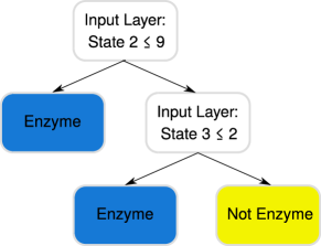
Figure 1: Final layer decision rule of DT+GNN for the PROTEINS dataset. This layer counts how many nodes representing certain chemical structures (states 2 and 3) the protein has. If there are not too many, the protein is an enzyme.

and their lack of human interpretability limits their use in many potential application areas. This motivated the adoption of existing deep learning explanation methods [2; 21; 37] to GNNs, and the creation of new GNN-specific methods [54; 47]. These methods allow us to understand what parts of the input were important for making a prediction. However, these methods do not explain how a GNN uses its inputs.

In this paper, we present a new fully explainable GNN architecture called Decision Tree GNN (DT+GNN). Fully explainable means that we can also inspect the decision making process and see how the GNN uses its inputs. For example, consider the output layer of DT+GNN for the PROTEINS dataset [4] in Figure 1. We see that DT+GNN simply counts the occurrences of certain chemical structures in the input graph to make its prediction. DT+GNN does not care at all how the amino acids are connected. In fact, this confirms a known observation that simple counting can outperform traditional GNNs on this dataset [13]. DT+GNN provides insights not only for PROTEINS but also for many other datasets. We discuss these for the BA-2Motifs [31], Tree-Cycle [54], and MUTAG[10] datasets in Section 4.3, and others in Appendix C. We summarize our contributions as follows:

• We propose a new differentiable Diff-DT+GNN layer. While traditional GNNs are based on a distributed computing model known as synchronous message passing [29], our new layer is based on a simplified distributed computing model known as the stone age model [12]. In this model, nodes use a small categorical space for states and messages. We argue that the stone age model is more suitable for interpretation while retaining a high theoretical expressiveness.

• We make our model fully interpretable by making use of decision trees. We first train Diff-DT+GNN using gradient descent. Internally, Diff-DT+GNN uses Multi-Layer Perceptrons (MLPs). Then, we replace each MLP with a decision tree while keeping the original GNN message passing structure. This gives us a model consisting of a series of decision tree layers, which makes it fully interpretable. We name our model Decision Tree GNN (DT+GNN).

• We propose a way to collectively prune the decision trees in DT+GNN without compromising accuracy. This leads to smaller trees, which further increases explainability.

• We further provide a way to extract traditional GNN explanations from DT+GNN. These explanations form a heat map that highlights the important nodes in the graph.

• We test our proposed architecture on established GNN explanation benchmarks and real-world graph datasets. We show our models are competitive in classification accuracy with traditional GNNs. We further validate that the proposed pruning methods considerably reduce tree sizes. We also demonstrate that DT+GNN can be used to discover problems in existing explanation benchmarks and to find interesting insights into real-world datasets.

• Finally, we provide a user interface for DT+GNN. This tool allows for the interactive exploration of the DT+GNN decision process on the datasets examined in this paper. We provide a manual for the interface in Appendix A.

2 Related Work

2.1 Explanation methods for GNNs

In recent years, several methods for providing GNN explanations were proposed. These methods highlight which parts of the input are important in a GNN decision. Generally, they explain a prediction either by assigning importance scores to nodes and edges or by finding similar predictions to help humans recognize patterns. The existing explanation methods can be roughly grouped into the following five groups:

Gradient based. Baldassarre and Azizpour [2] and Pope et al. [37] show that it is possible to adopt gradient-based methods that we know from computer vision, for example Grad-CAM[44], to graphs. Gradients can be computed on node features and edges [43].
Mutual-Information based. Ying et al. [54] also measure the importance of edges and node features. Edges are masked with continuous values. Instead of gradients, the authors use mutual information between inputs and the prediction to quantify the impact. Luo et al. [31] follow a similar idea but emphasize finding important edges and finding explanations for many predictions at the same time.
Subgraph based. Yuan et al. [56] search the space of all subgraphs as possible explanations. To score a subgraph, they use Shapley values [46] and monte carlo tree search for guiding the search. Duval and Malliaros [11] build subgraphs by masking nodes and edges in the graph. They run their subgraph through the trained GNN and try to explain the differences to the entire graph with simple interpretable models and Shapley values. Zhang et al. [57] infer subgraphs called prototypes that each map to one particular class. Graphs are classified through their similarity to the prototypes.
Example based. Huang et al. [21] proposes a graph version of the LIME [39] algorithm. A prediction is explained through a linear decision boundary built by close-by examples. Vu and Thai [47] aim to capture the dependencies in node predictions and express them in probabilistic graphical models. Faber et al. [14] explain a node by giving examples of similar nodes with the same and different labels. Dai and Wang [8] create a $k$-nearest neighbor model and use GNNs to create the feature space to compute similarities in.
Simple GNNs. Another interesting line of research are simplified GNN architectures [6; 7; 22]. The main goal of this research is to show that simple architectures can perform competitively with traditional, complex ones. As a side effect, the simplicity of these architectures also makes them slightly more understandable.

Complimentary to the development of explanations methods is the research on how we can best evaluate them. Sanchez-Lengeling et al. [41] and Yuan et al. [55] discuss desirable properties a good explanation method should have. For example, an explanation method should be faithful to the model, which means that an explanation method should reflect the model’s performance and behavior. Agarwal et al. [1] provide a theoretical framework to define how strong explanation methods adhere to these properties. They also derive bounds for several explanation methods. Faber et al. [15] and Himmelhuber et al. [19] discuss deficiencies in the existing benchmarks used for empirical evaluation.

Note that all these methods do not provide full explainability. They can show us the important nodes and edges a GNN uses to predict. But (in contrast to DT+GNN) they cannot give insights into the GNN’s decision making process itself.

2.2 Decision trees for neural networks

Decision trees are powerful machine learning methods, which in some tasks rival the performance of neural networks [18]. The cherry on top is their inherent interpretability. Therefore, researchers have tried to distill neural networks into trees to make them explainable [5; 9; 28]. More recently, Schaaf et al. [42] have shown that encouraging sparsity and orthogonality in neural network weight matrices allows for model distillation into smaller trees with higher final accuracy. Wu et al. [49] follow a similar idea for time series data: they regularize the training process for recurrent neural networks to penalize weights that cannot be modeled easily by complex decision trees. Yang et al. [53] aim to directly learn neural trees. Their neural layers learn how to split the data and put it into bins. Stacking these layers creates trees. Kontschieder et al. [27] learn neural decision forests by making the routing in nodes probabilistic and learning these probabilities and the leaf predictions.

Our DT+GNN follows the same underlying idea: we want to structure a GNN in a way that allows for model distillation into decision trees to leverage their interpretability. However, the graph setting brings additional challenges. We not only have feature matrices for each node, but we also need to allow the trees to reason about the state of neighboring nodes one or more hops away.

3 The DT+GNN Model

3.1 The Diff-DT+GNN layer

Loukas [29] show that GNNs operate very similar to synchronous message passing algorithms from distributed computing. Often, these algorithms have a limit on the message size of $b=O(\log n)$ bits (where $n$ is the number of nodes) but can perform arbitrary local computation [36]. In contrast to this, the stone age distributed computing model [12] assumes that each node uses a finite state machine to update its state and send its updated state as a message to all neighbors. The receiving node can count the number of neighbors in each state. A stone age node cannot even count arbitrarily, it can only count up to a predefined number, in the spirit of “one, two, many”. Neighborhood counts above a threshold are indistinguishable from each other. Interestingly enough, such a simplified model can still solve many distributed computing problems [12].

Clearly, this simplified model would also be easier to interpret. We create the Diff-DT+GNN layer similar to this model (Figure 2) which is fully differentiable. The layer largely follows traditional message passing [17]. Nodes update their state through an UPDATE function that takes the aggregated messages $M$ from neighbors and the node’s current state $S$ as input. To retain differentiability, this layer uses MLPs instead of finite state machines in the UPDATE step. We constrain the output space of the UPDATE step to be categorical, by using a Gumbel-Softmax [24; 32]. Similarly to models like GIN [51], every node sends its state directly to its neighbors. Together with sum aggregation, this allows each node to count neighbor states, as in the stone age model. However, we deviate from the stone age model by not restricting the neighborhood counting. We find this produces better results without sacrificing interpretability.

In principle, the categorical state space also does not reduce expressiveness. Using a GNN with messages that have $O(\log{n})$ bits is equivalent to using categorical messages with $O(n)$ bits. Practically, we are interested in small interpretable state spaces, and hence, we constrain the state space to small values. The reduced expressiveness does not impact the performance in practice (c.f., Table LABEL:tab:accuracies).

We can now build Diff-DT+GNN from these layers. We add an encoder MLP at the beginning that projects the input features into a categorical space. We append a decoder MLP at the end that works on a concatenation of intermediate outputs. For node classification, the decoder concatenates node states; for graph classification, the decoder concatenates the pooled state counts.

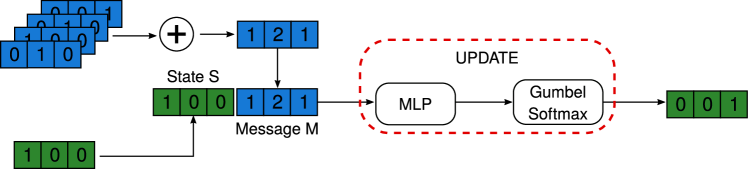
Figure 2: A Diff-DT+GNN layer. It follows normal message passing layers to a large extend, except it computes a categorical state in the end, instead of a real-valued embedding vector.

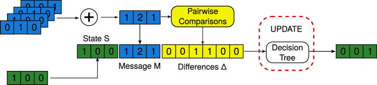
Figure 3: A DT+GNN layer. We replace the UPDATE of a Diff-DT+GNN layer with a decision tree. DT+GNN receive additional $\Delta$ features to compare two features.

3.2 Distilling the DT+GNN

Using an MLP in the UPDATE step harms explainability. To fix this, we distill all of the MLPs used in the GNN, including the encoder and decoder MLPs, into decision trees. To train the decision trees, we pass all of the training graphs through the Diff-DT+GNN model and record all inputs and outputs for every UPDATE block. Then, we train a decision tree to replace each block predicting the outputs from inputs. Thanks to the categorical states, this is a classification problem.

Unlike MLPs, decision trees cannot easily compare two features. Decision trees can compare them by building a binary tree but such trees quickly become large and hard to understand. To produce small trees, we include pairwise delta features $\Delta$, binary features for the count comparisons for every pair of states. With all MLPs replaced with decision trees, we now have a fully interpretable architecture.

Figure 3 shows a layer in our architecture using such decision trees. These trees define how we determine the next state for each node. The decision trees can use three different types of branching criteria for every decision node. Figure 4 shows an example branch of every type.

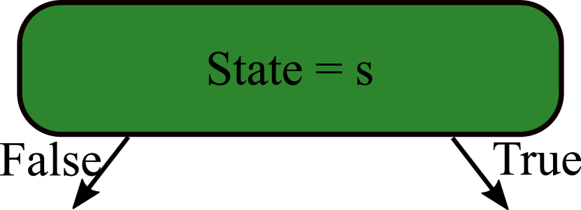
(a)

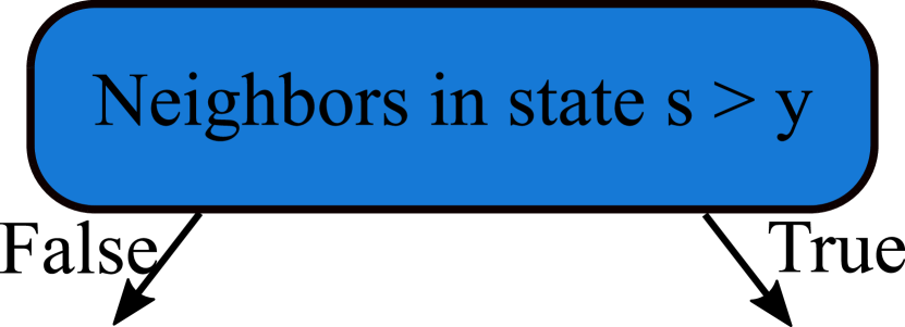
(b)

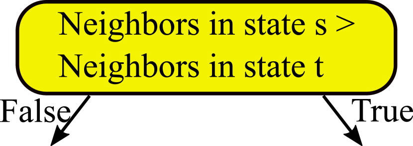
(c)

Figure 4: The different branches possible in a DT+GNN layer. We can branch on (a) the state a node is in, (b) if the node has a certain number of neighbors in a certain state, or (c) if the node has more neighbors in one state than another state.

With the state features $\in S$, we can branch on whether or not a node is in a particular state $s$ at the beginning of the layer (Figure 4(a)). Using a message feature $\in M$, a decision node branches if a node has more than $y$ neighbors in state $s$, $y$ is learnable (Figure 4(b)). Last, we can use branch with a delta feature $\in\Delta$ on whether a node has more neighbors in state $s$ than in state $t$ (Figure 4(c)).

3.3 Postprocessing the DT+GNN

While decision trees, like MLPs, are universal function approximators if they are sufficiently deep [40], we aim to have shallow decision trees. Shallow trees are more akin to the finite state machine used in the stone age distributed computing model and are more explainable. We directly put a cap on the number of decision leaves per tree.

Lossless pruning.

We prune more nodes based on the reduced error pruning algorithm [38]. First, we define a set of data points used for pruning (pruning set). Then, we assess every decision node, starting with the one that acts upon the fewest data points. If replacing the decision node with a leaf does not lead to an accuracy drop over the entire DT+GNN on the pruning set, we replace it. We keep iterating through all decision nodes until no more changes are made.

Choosing the pruning set is not trivial. If we use the training set for pruning, all of the overfitted edge cases with few samples are used and not pruned. On the other hand, the much smaller validation set might not cover all of the decision paths and cause overpruning. Therefore, we propose to prune on both training and validation set with a different pruning criterion: A node can be pruned if replacing it with a leaf does not reduce the validation set accuracy (as in reduced error pruning) and does not reduce the training set accuracy below the validation set accuracy. Not allowing a validation accuracy drop ensures that we do not overprune. But since we allow a drop in training accuracy for the modified tree, we also remove decision nodes that result from overfitting.

Lossy Pruning.

Empirically, we found that we can prune substantially more decision nodes when we allow for a slight deterioration in the validation accuracy. We follow the same approach as before and always prune the decision node that leads to the smallest deterioration. We repeat this until we are satisfied with the tradeoff between the model accuracy and tree size. Defining this tradeoff is difficult as it is subjective and specific to each dataset. Therefore, we included a feature in our user interface that allows users to try different pruning steps and report the impact on accuracy. These steps are incrementally pruning $10\%$ of the nodes in the losslessly pruned decision tree.

3.4 Generating Explanations

We can use DT+GNN to create node importances as explanations similar to existing explanation methods. Formally, such an explanation $e^{l}_{(v,t)}\in\mathbb{R}^{n}$ assigns each node a real-valued importance, how much it contributed to node $v$ being in state $t$ in layer $l$. Final explanations are then taken from the final decoder layer, where states equate to classes.

We derive these explanations in a propagation procedure similar to the forward pass of a graph neural network. Initially, every node is solely responsible for its encoded state, so the initial explanation for node $v$ is $e^{0}_{(v,t)}$, which is a one-hot vector that is $1$ at the $v-$position, for all states $t$. But as nodes interact with their neighbors, we need to propagate explanations. Let us consider a DT+GNN layer $l$ that maps from the input state space $S$ to the target space $T$. We need to (i) understand the importance of each input feature for the decision tree, and (ii) map the importance of decision tree features back to graph nodes. For (i) we can use the Shapley values obtained by the TreeShap algorithm [30] to assign an importance score for all features in $S,M,\Delta$ for every target state $t$. We compute these scores per node to have node-specific explanations. We can represent the TreeShap importance in three matrices $I^{l}_{S}\in\mathbb{R}^{n\times T\times S}$, $I^{l}_{M}\in\mathbb{R}^{n\times T\times S}$, $I^{l}_{\Delta}\in\mathbb{R}^{n\times T\times(S^{2}-S)}$. For (ii) we need to differentiate the type of feature to understand its propagation.

Propagating State Feature Explanations.

Propagating explanations of one of the $S$ state features is easiest since it does not involve other nodes. The new explanation is the sum over the input state explanations, weighted by their matching feature Shapley value. There is one catch: For a state branching criterion, it can be important to not be in a certain state, which requires inverting the explanations. We define the indicator variable $sign(s)$ which is $+1$ if node $v$ is in the input state $s$, otherwise it is $-1$. We multiply the indicator with the explanation:

$$\sigma^{l+1}_{(v,t)}=\sum_{s\in S}I^{l}_{S}[v,t,s]\cdot e^{l}_{(v,s)}\cdot sign(s).$$

Propagating Message Feature Explanations.

When one of the message features is used, the node depends on the number of neighbors in the state mapping to the message feature. Let $N_{s}(v)$ denote the set of neighbors of node $v$ that have input state $s$. The node explanation becomes the average of the explanations of the nodes in $N_{s}(v)$. We can compute the next explanation by summing this expression over all input states $S$:

$$\mu^{l+1}_{(v,t)}=\sum_{s\in S}I^{l}_{M}[v,t,s]\cdot\sum_{w\in N_{s}(v)}\frac{e^{l}_{(w,s)}}{|N_{s}(v)|}.$$

Propagating Delta Feature Explanations.

Let us consider propagation for the feature $f(s,s^{\prime})$ that is $1$ if there are more neighbors of input state $s$ than $s^{\prime}$. The neighbors in $N_{s}(v)$ propagate explanations the same way as for a message feature. On the other hand, the nodes in $N_{s^{\prime}}(v)$ work against setting $f$ to true, so we subtract their explanations. If there are more neighbors with an input state $s^{\prime}$ than $s$ we have to flip the explanations of which neighbors contribute positively and negatively, for this we introduce the indicator variable $\mathbbm{1}_{>({s,s^{\prime}})}$ that is either $+1$ or $-1$:

$$\delta^{l+1}_{(v,s)}=\sum_{s\in S}\sum_{s^{\prime}\neq s\in S}I^{l}_{\Delta}[v,t,f(s,s^{\prime})]\frac{\sum_{w\in N_{s}(v)}e^{l}_{(w,s)}-\sum_{w\in N_{s^{\prime}}(v)}e^{l}_{(w,s^{\prime})}}{|N_{s}(v)|+|N_{s^{\prime}}(v)|}\cdot\mathbbm{1}_{>({s,s^{\prime}})}.$$

The node state explanations for the next layer are the sum of these three components:

$$e^{l+1}_{(v,s)}=\sigma^{l+1}_{(v,t)}+\mu^{l+1}_{(v,t)}+\delta^{l+1}_{(v,s)}.$$

The decoder layer is slightly special since its input features are the concatenation of node states (or node state counts for graph classification) from all other layers. For node classification, we directly compute the decoder’s explanation from the respective layers. However, for graph classification the node states are pooled as follows: We supply the decoder with node state counts and count deltas as features, equivalent to the $M$ and $\Delta$ features in the DT+GNN layers. The only difference is that instead of propagating the explanation from neighbors, we now need to propagate it from all of the nodes in the graph that were in the corresponding states.

4 Experiments

4.1 Experiment setup

Datasets.

We conduct experiments on two different types of datasets. First, we run DT+GNN on synthetic GNN explanation benchmarks introduced by previous literature. We use the Infection and Negative Evidence benchmarks from Faber et al. [15], The BA-Shapes, Tree-Cycle, and Tree-Grid benchmarks from Ying et al. [54], and the BA-2Motifs dataset from Luo et al. [31]. For all of these datasets, we know why a graph or a node should be in a particular class. This allows us to verify that the model makes correct decisions and we compute correct explanations. Second, we experiment with the following real-world datasets: MUTAG [10]; BBBP [50]; Mutagenicity [26]; PROTEINS, REDDIT-BINARY, IMDB-BINARY, and COLLAB [4]. We provide more information for all datasets, such as statistics, descriptions, and examples in Appendix B. Note that all datasets are small which allows training on a few commodity CPUs. The tree construction needs little extra computation, and the cost of tree pruning is also clearly dominated by GNN training time. Precomputing all thresholds for the lossy pruning took noticeable additional time, which we sped up with a GPU for some of the larger datasets (for example, COLLAB or REDDIT-BINARY).

Training and Hyperparameters.

We follow the same training scheme for all datasets following existing works [51]. We do a $10-$fold cross validation of the data with different splits and train both DT+GNN and a baseline GIN architecture. Both GNNs use a $2-$ layer MLP for the update function, with batch normalization [23] and ReLu[33] in between the two linear layers. GIN uses a hidden dimension of $16$, DT+GNN uses a state space of $10$. We also further divide the training set for DT+GNN to keep a holdout set for pruning decision trees. After we train Diff-DT+GNN with Gradient Descent we distill the MLPs inside into decision trees. Each tree is limited to have a maximum of $100$ nodes. The GNNs are trained on the training set for $1500$ epochs, allowing early stopping on the validation loss with a patience of $100$. Each split uses early stopping on the validation score, the results are averaged over the $10$ splits.

DT+GNN explainability allows us to see if DT+GNN uses all layers and available states. When we see unused states in the decision trees and that layers are skipped, we retrain DT+GNN with the number of layers and states that were actually used. The retrained model does not improve accuracy but it is smaller and more interpretable. We show these in Table LABEL:tab:hyperparam. A full model is used for GIN.

4.2 Quantitative Results

DT+GNN performs comparably to GIN.

First, we investigate the two assumptions that (i) Diff-DT+GNN matches the performance of GIN and (ii) that converting from Diff-DT+GNN to DT+GNN also comes with little loss in accuracy. We further investigate how pruning impacts DT+GNN accuracy. In Table LABEL:tab:accuracies we report the average test set accuracy for a GIN-based GNN, Diff-DT+GNN, DT+GNN with no pruning, and the lossless version of our pruning method.

We find that DT+GNN performs almost identically to GIN. The model simplifications which increase explainability do not decrease accuracy. We observe, that tree pruning even tends to have a positive effect on test accuracy compared to non-pruned DT+GNN. This is likely due to the regularization induced by the pruning procedure.

		DT+GNN
Dataset	GIN	Differentiable	No pruning	Lossless pruning
Infection	$0.98\raisebox{0.86108pt}{$\scriptstyle\pm$}0.04$	$1.00\raisebox{0.86108pt}{$\scriptstyle\pm$}0.00$	$1.00\raisebox{0.86108pt}{$\scriptstyle\pm$}0.00$	$1.00\raisebox{0.86108pt}{$\scriptstyle\pm$}0.00$
Negative	$1.00\raisebox{0.86108pt}{$\scriptstyle\pm$}0.00$	$1.00\raisebox{0.86108pt}{$\scriptstyle\pm$}0.00$	$1.00\raisebox{0.86108pt}{$\scriptstyle\pm$}0.00$	$1.00\raisebox{0.86108pt}{$\scriptstyle\pm$}0.00$
BA-Shapes	$0.97\raisebox{0.86108pt}{$\scriptstyle\pm$}0.02$	$1.00\raisebox{0.86108pt}{$\scriptstyle\pm$}0.01$	$0.99\raisebox{0.86108pt}{$\scriptstyle\pm$}0.01$	$0.99\raisebox{0.86108pt}{$\scriptstyle\pm$}0.01$
Tree-Cycles	$1.00\raisebox{0.86108pt}{$\scriptstyle\pm$}0.00$	$1.00\raisebox{0.86108pt}{$\scriptstyle\pm$}0.00$	$1.00\raisebox{0.86108pt}{$\scriptstyle\pm$}0.00$	$1.00\raisebox{0.86108pt}{$\scriptstyle\pm$}0.00$
Tree-Grid	$1.00\raisebox{0.86108pt}{$\scriptstyle\pm$}0.01$	$0.99\raisebox{0.86108pt}{$\scriptstyle\pm$}0.01$	$0.99\raisebox{0.86108pt}{$\scriptstyle\pm$}0.01$	$0.99\raisebox{0.86108pt}{$\scriptstyle\pm$}0.01$
BA-2Motifs	$1.00\raisebox{0.86108pt}{$\scriptstyle\pm$}0.00$	$1.00\raisebox{0.86108pt}{$\scriptstyle\pm$}0.00$	$1.00\raisebox{0.86108pt}{$\scriptstyle\pm$}0.00$	$1.00\raisebox{0.86108pt}{$\scriptstyle\pm$}0.00$
MUTAG	$0.88\raisebox{0.86108pt}{$\scriptstyle\pm$}0.05$	$0.88\raisebox{0.86108pt}{$\scriptstyle\pm$}0.06$	$0.88\raisebox{0.86108pt}{$\scriptstyle\pm$}0.06$	$0.85\raisebox{0.86108pt}{$\scriptstyle\pm$}0.08$
Mutagenicity	$0.81\raisebox{0.86108pt}{$\scriptstyle\pm$}0.02$	$0.79\raisebox{0.86108pt}{$\scriptstyle\pm$}0.02$	$0.75\raisebox{0.86108pt}{$\scriptstyle\pm$}0.02$	$0.74\raisebox{0.86108pt}{$\scriptstyle\pm$}0.02$
BBBP	$0.81\raisebox{0.86108pt}{$\scriptstyle\pm$}0.04$	$0.83\raisebox{0.86108pt}{$\scriptstyle\pm$}0.03$	$0.82\raisebox{0.86108pt}{$\scriptstyle\pm$}0.03$	$0.83\raisebox{0.86108pt}{$\scriptstyle\pm$}0.03$
PROTEINS	$0.70\raisebox{0.86108pt}{$\scriptstyle\pm$}0.03$	$0.71\raisebox{0.86108pt}{$\scriptstyle\pm$}0.02$	$0.71\raisebox{0.86108pt}{$\scriptstyle\pm$}0.04$	$0.71\raisebox{0.86108pt}{$\scriptstyle\pm$}0.04$
IMDB-B	$0.69\raisebox{0.86108pt}{$\scriptstyle\pm$}0.04$	$0.70\raisebox{0.86108pt}{$\scriptstyle\pm$}0.05$	$0.69\raisebox{0.86108pt}{$\scriptstyle\pm$}0.03$	$0.69\raisebox{0.86108pt}{$\scriptstyle\pm$}0.04$
REDDIT-B	$0.87\raisebox{0.86108pt}{$\scriptstyle\pm$}0.10$	$0.90\raisebox{0.86108pt}{$\scriptstyle\pm$}0.03$	$0.88\raisebox{0.86108pt}{$\scriptstyle\pm$}0.03$	$0.87\raisebox{0.86108pt}{$\scriptstyle\pm$}0.04$
COLLAB	$0.72\raisebox{0.86108pt}{$\scriptstyle\pm$}0.01$	$0.70\raisebox{0.86108pt}{$\scriptstyle\pm$}0.02$	$0.69\raisebox{0.86108pt}{$\scriptstyle\pm$}0.02$	$0.69\raisebox{0.86108pt}{$\scriptstyle\pm$}0.02$

(a)

Hyperparameters
Layers	States
$5$	$6$
$1$	$3$
$5$	$5$
$5$	$5$
$5$	$5$
$4$	$6$
$4$	$6$
$3$	$8$
$3$	$5$
$3$	$5$
$3$	$5$
$3$	$5$
$3$	$8$

(b)

Table 1: a) Test set accuracies using different GNN layers. All methods perform virtually the same for all datasets. This shows that DT+GNN layers match the expressiveness of GIN in practice. (b) DT+GNN hyperparameters found through tree inspection.

Pruning significantly reduces the decision tree sizes.

Second, we examine the effectiveness of our pruning method. We compare the tree sizes before pruning, after lossless pruning, and after lossy pruning. We measure tree size as the sum of decision nodes over all trees. Additionally, we verify the effectiveness of using our pruning criterion for reduced error pruning and compare it against simpler setups of using only the training or validation set for pruning. We report the tree sizes and test set accuracies for all configurations in Table 2.

We can see that the reduced error pruning leads to an impressive drop in the number of nodes required in the decision trees. On average, we can prune about $62\%$ of nodes in synthetic datasets and even around $84\%$ of nodes in real-world datasets without a loss in accuracy. If we accept small drops, in accuracy we can even a total of $68\%$ and $87\%$ of nodes in synthetic and real-world datasets, respectively. If we compare the different approaches for reduced error pruning, we can see that our proposed approach of using both training and validation accuracy performs the best. As expected, pruning only on the validation set tends to overprune the trees: Trees become even smaller but there is also a larger drop in accuracy, especially in the real-world datasets. Using the training set tends to underprune, there is no drop in accuracy but decision trees for real-world graphs tend to stay large.

	No pruning		REP Training		REP Validation		REP Ours		REP Lossy
Dataset	Accuracy	Size	Accuracy	Size	Accuracy	Size	Accuracy	Size	Accuracy	Size
Infection	$1.00\raisebox{0.86108pt}{$\scriptstyle\pm$}0.00$	$205\raisebox{0.86108pt}{$\scriptstyle\pm$}56$	$1.00\raisebox{0.86108pt}{$\scriptstyle\pm$}0.00$	$26\raisebox{0.86108pt}{$\scriptstyle\pm$}2$	$1.00\raisebox{0.86108pt}{$\scriptstyle\pm$}0.00$	$25\raisebox{0.86108pt}{$\scriptstyle\pm$}2$	$1.00\raisebox{0.86108pt}{$\scriptstyle\pm$}0.00$	$26\raisebox{0.86108pt}{$\scriptstyle\pm$}2$	$0.98\raisebox{0.86108pt}{$\scriptstyle\pm$}0.01$	$17\raisebox{0.86108pt}{$\scriptstyle\pm$}2$
Negative	$1.00\raisebox{0.86108pt}{$\scriptstyle\pm$}0.00$	$18\raisebox{0.86108pt}{$\scriptstyle\pm$}14$	$1.00\raisebox{0.86108pt}{$\scriptstyle\pm$}0.00$	$5\raisebox{0.86108pt}{$\scriptstyle\pm$}0$	$1.00\raisebox{0.86108pt}{$\scriptstyle\pm$}0.00$	$5\raisebox{0.86108pt}{$\scriptstyle\pm$}0$	$1.00\raisebox{0.86108pt}{$\scriptstyle\pm$}0.00$	$5\raisebox{0.86108pt}{$\scriptstyle\pm$}0$	$1.00\raisebox{0.86108pt}{$\scriptstyle\pm$}0.00$	$4\raisebox{0.86108pt}{$\scriptstyle\pm$}0$
BA-Shapes	$0.99\raisebox{0.86108pt}{$\scriptstyle\pm$}0.01$	$30\raisebox{0.86108pt}{$\scriptstyle\pm$}10$	$0.99\raisebox{0.86108pt}{$\scriptstyle\pm$}0.01$	$21\raisebox{0.86108pt}{$\scriptstyle\pm$}5$	$0.97\raisebox{0.86108pt}{$\scriptstyle\pm$}0.03$	$15\raisebox{0.86108pt}{$\scriptstyle\pm$}4$	$0.99\raisebox{0.86108pt}{$\scriptstyle\pm$}0.01$	$21\raisebox{0.86108pt}{$\scriptstyle\pm$}5$	$0.98\raisebox{0.86108pt}{$\scriptstyle\pm$}0.04$	$17\raisebox{0.86108pt}{$\scriptstyle\pm$}4$
Tree-Cycles	$1.00\raisebox{0.86108pt}{$\scriptstyle\pm$}0.00$	$19\raisebox{0.86108pt}{$\scriptstyle\pm$}5$	$1.00\raisebox{0.86108pt}{$\scriptstyle\pm$}0.00$	$11\raisebox{0.86108pt}{$\scriptstyle\pm$}3$	$0.99\raisebox{0.86108pt}{$\scriptstyle\pm$}0.02$	$9\raisebox{0.86108pt}{$\scriptstyle\pm$}2$	$1.00\raisebox{0.86108pt}{$\scriptstyle\pm$}0.00$	$11\raisebox{0.86108pt}{$\scriptstyle\pm$}3$	$0.99\raisebox{0.86108pt}{$\scriptstyle\pm$}0.01$	$9\raisebox{0.86108pt}{$\scriptstyle\pm$}3$
Tree-Grid	$0.99\raisebox{0.86108pt}{$\scriptstyle\pm$}0.01$	$30\raisebox{0.86108pt}{$\scriptstyle\pm$}13$	$0.99\raisebox{0.86108pt}{$\scriptstyle\pm$}0.01$	$17\raisebox{0.86108pt}{$\scriptstyle\pm$}8$	$0.99\raisebox{0.86108pt}{$\scriptstyle\pm$}0.01$	$13\raisebox{0.86108pt}{$\scriptstyle\pm$}4$	$0.99\raisebox{0.86108pt}{$\scriptstyle\pm$}0.01$	$15\raisebox{0.86108pt}{$\scriptstyle\pm$}8$	$0.99\raisebox{0.86108pt}{$\scriptstyle\pm$}0.01$	$15\raisebox{0.86108pt}{$\scriptstyle\pm$}8$
BA-2Motifs	$1.00\raisebox{0.86108pt}{$\scriptstyle\pm$}0.00$	$141\raisebox{0.86108pt}{$\scriptstyle\pm$}43$	$1.00\raisebox{0.86108pt}{$\scriptstyle\pm$}0.00$	$12\raisebox{0.86108pt}{$\scriptstyle\pm$}3$	$1.00\raisebox{0.86108pt}{$\scriptstyle\pm$}0.01$	$11\raisebox{0.86108pt}{$\scriptstyle\pm$}3$	$1.00\raisebox{0.86108pt}{$\scriptstyle\pm$}0.00$	$13\raisebox{0.86108pt}{$\scriptstyle\pm$}4$	$1.00\raisebox{0.86108pt}{$\scriptstyle\pm$}0.00$	$13\raisebox{0.86108pt}{$\scriptstyle\pm$}4$
MUTAG	$0.88\raisebox{0.86108pt}{$\scriptstyle\pm$}0.06$	$59\raisebox{0.86108pt}{$\scriptstyle\pm$}27$	$0.86\raisebox{0.86108pt}{$\scriptstyle\pm$}0.08$	$19\raisebox{0.86108pt}{$\scriptstyle\pm$}17$	$0.83\raisebox{0.86108pt}{$\scriptstyle\pm$}0.07$	$7\raisebox{0.86108pt}{$\scriptstyle\pm$}6$	$0.85\raisebox{0.86108pt}{$\scriptstyle\pm$}0.08$	$18\raisebox{0.86108pt}{$\scriptstyle\pm$}16$	$0.85\raisebox{0.86108pt}{$\scriptstyle\pm$}0.08$	$18\raisebox{0.86108pt}{$\scriptstyle\pm$}16$
Mutagenicity	$0.75\raisebox{0.86108pt}{$\scriptstyle\pm$}0.02$	$375\raisebox{0.86108pt}{$\scriptstyle\pm$}13$	$0.76\raisebox{0.86108pt}{$\scriptstyle\pm$}0.02$	$154\raisebox{0.86108pt}{$\scriptstyle\pm$}19$	$0.73\raisebox{0.86108pt}{$\scriptstyle\pm$}0.01$	$56\raisebox{0.86108pt}{$\scriptstyle\pm$}16$	$0.74\raisebox{0.86108pt}{$\scriptstyle\pm$}0.02$	$91\raisebox{0.86108pt}{$\scriptstyle\pm$}36$	$0.73\raisebox{0.86108pt}{$\scriptstyle\pm$}0.02$	$50\raisebox{0.86108pt}{$\scriptstyle\pm$}19$
BBBP	$0.82\raisebox{0.86108pt}{$\scriptstyle\pm$}0.03$	$366\raisebox{0.86108pt}{$\scriptstyle\pm$}53$	$0.84\raisebox{0.86108pt}{$\scriptstyle\pm$}0.02$	$88\raisebox{0.86108pt}{$\scriptstyle\pm$}52$	$0.79\raisebox{0.86108pt}{$\scriptstyle\pm$}0.04$	$8\raisebox{0.86108pt}{$\scriptstyle\pm$}10$	$0.83\raisebox{0.86108pt}{$\scriptstyle\pm$}0.03$	$46\raisebox{0.86108pt}{$\scriptstyle\pm$}27$	$0.82\raisebox{0.86108pt}{$\scriptstyle\pm$}0.03$	$31\raisebox{0.86108pt}{$\scriptstyle\pm$}18$
PROTEINS	$0.71\raisebox{0.86108pt}{$\scriptstyle\pm$}0.04$	$206\raisebox{0.86108pt}{$\scriptstyle\pm$}90$	$0.72\raisebox{0.86108pt}{$\scriptstyle\pm$}0.03$	$12\raisebox{0.86108pt}{$\scriptstyle\pm$}13$	$0.70\raisebox{0.86108pt}{$\scriptstyle\pm$}0.04$	$8\raisebox{0.86108pt}{$\scriptstyle\pm$}6$	$0.71\raisebox{0.86108pt}{$\scriptstyle\pm$}0.04$	$9\raisebox{0.86108pt}{$\scriptstyle\pm$}6$	$0.71\raisebox{0.86108pt}{$\scriptstyle\pm$}0.04$	$9\raisebox{0.86108pt}{$\scriptstyle\pm$}6$
IMDB-B	$0.69\raisebox{0.86108pt}{$\scriptstyle\pm$}0.03$	$218\raisebox{0.86108pt}{$\scriptstyle\pm$}32$	$0.69\raisebox{0.86108pt}{$\scriptstyle\pm$}0.04$	$20\raisebox{0.86108pt}{$\scriptstyle\pm$}9$	$0.66\raisebox{0.86108pt}{$\scriptstyle\pm$}0.06$	$16\raisebox{0.86108pt}{$\scriptstyle\pm$}6$	$0.69\raisebox{0.86108pt}{$\scriptstyle\pm$}0.04$	$29\raisebox{0.86108pt}{$\scriptstyle\pm$}9$	$0.69\raisebox{0.86108pt}{$\scriptstyle\pm$}0.04$	$29\raisebox{0.86108pt}{$\scriptstyle\pm$}9$
REDDIT-B	$0.88\raisebox{0.86108pt}{$\scriptstyle\pm$}0.03$	$248\raisebox{0.86108pt}{$\scriptstyle\pm$}28$	$0.88\raisebox{0.86108pt}{$\scriptstyle\pm$}0.02$	$53\raisebox{0.86108pt}{$\scriptstyle\pm$}14$	$0.85\raisebox{0.86108pt}{$\scriptstyle\pm$}0.04$	$28\raisebox{0.86108pt}{$\scriptstyle\pm$}8$	$0.87\raisebox{0.86108pt}{$\scriptstyle\pm$}0.04$	$49\raisebox{0.86108pt}{$\scriptstyle\pm$}21$	$0.87\raisebox{0.86108pt}{$\scriptstyle\pm$}0.04$	$38\raisebox{0.86108pt}{$\scriptstyle\pm$}15$
COLLAB	$0.69\raisebox{0.86108pt}{$\scriptstyle\pm$}0.02$	$301\raisebox{0.86108pt}{$\scriptstyle\pm$}1$	$0.70\raisebox{0.86108pt}{$\scriptstyle\pm$}0.02$	$36\raisebox{0.86108pt}{$\scriptstyle\pm$}15$	$0.67\raisebox{0.86108pt}{$\scriptstyle\pm$}0.03$	$22\raisebox{0.86108pt}{$\scriptstyle\pm$}12$	$0.69\raisebox{0.86108pt}{$\scriptstyle\pm$}0.02$	$30\raisebox{0.86108pt}{$\scriptstyle\pm$}18$	$0.68\raisebox{0.86108pt}{$\scriptstyle\pm$}0.02$	$21\raisebox{0.86108pt}{$\scriptstyle\pm$}12$

Table 2: Running reduced error pruning (REP) on different pruning sets. Lossy prunes the nodes with least loss in accuracy up to a manually chosen threshold.

4.3 Qualitative Results

Bias Terms. Bias terms are often overlooked but can be problematic for importance explanations [48]. When a GNN uses bias terms to predict a class, nothing of the input was used so nothing should be important [15]. We observe this in the BA-2Motifs dataset. In this dataset, a GNN needs to predict if a given graph contains a house structure or a cycle. Figure 6(a) shows the output layer of DT+GNN for this dataset. If at least $5$ nodes are in the house (in state $2$ in layer $2$), the graph is classified as house, otherwise, it is a cycle. DT+GNN only learns what a house is, cycles are then “not houses”. Consequently, the explanations for which nodes contribute to the classification as a house are correct (Figure 6(b)) but the explanations for cycles are not (Figure 6(c)).

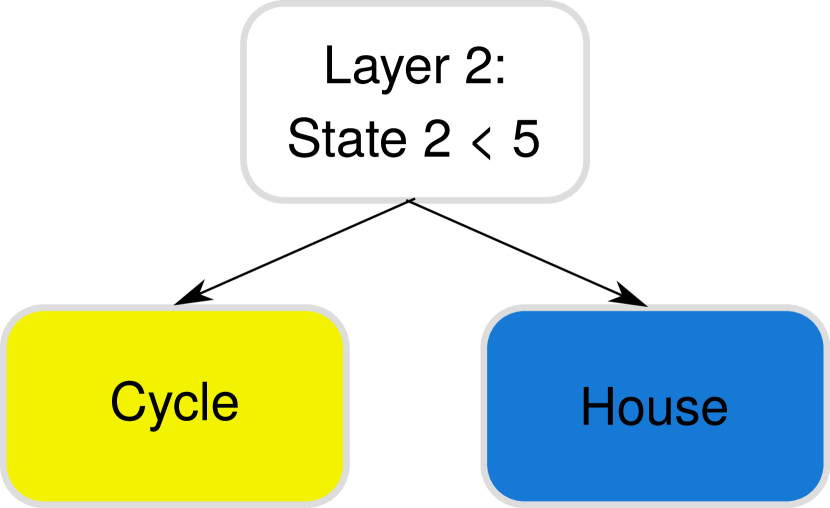
(a)

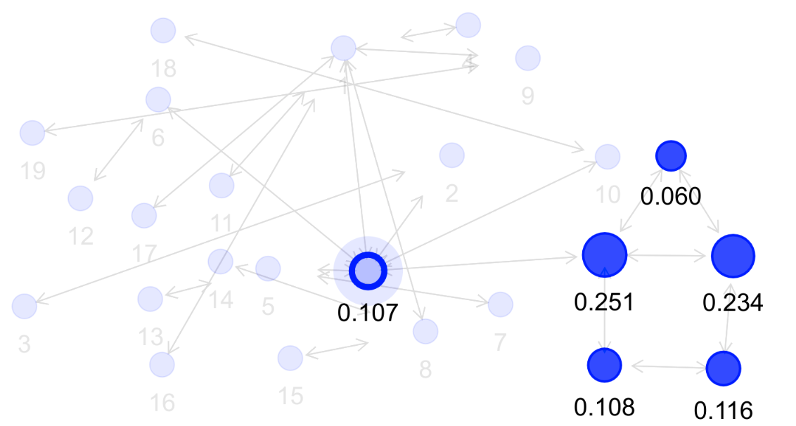
(b)

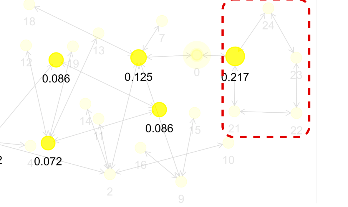
(c)

Figure 6: DT+GNN uses bias terms to solve the BA-2Motifs dataset. (a) The decoder layer only learns what a house is, the cycle is “not” a house (b) and (c) Explanation graphs: numbers denote the importance of each node, non-important nodes are transparent. (b) Correct explanation for the house on the right since all nodes in the house receive a high importance. (c) Incorrect explanation for the cycle in the the dashed red box since only one node in the cycle receives a high importance.

Surplus ground truth. Faber et al. [15] discuss that having more ground truth evidence than necessary can also cause problems with explanations. For example, we observe this problem on the Tree-Cycle dataset. DT+GNN uses the second layer for making the final prediction. At this point, no node could even see the whole cycle. This is because the base graph is a balanced binary tree. Apart from the root node, no nodes other than cycle nodes have degree $2$. In principle, DT+GNN learns to predict cycle nodes as those nodes having degree $2$ neighbors (Figure 7(a) and 7(b)). For a node $n$, DT+GNN assigns explanations to the nodes causing $n$ to have degree $2$ neighbors. Figure 7(c) shows an example explanation. The explanation for the highlighted node is the neighbors of its neighbors, the other cycle nodes are unnecessary. Therefore, they are not and should not be part of the explanation.

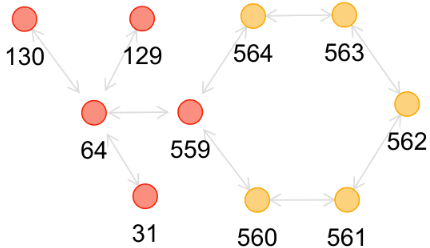
(a)

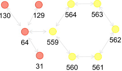
(b)

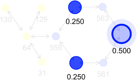
(c)

Figure 7: DT+GNN solves an instance of the Tree-Cycle dataset. (a) and (b) DT+GNN learns states for all nodes. Numbers are node IDs, different colors map to states. (a) DT+GNN finds nodes with a degree of $2$. (b) DT+GNN finds nodes connected to degree $2$ nodes, this already distinguishes the cycle from the remaining graph. (c) Explanations for the rightmost node, high numbers show nodes which important for that node’s final state. The correct explanation are the neighbors of the neighbors.

Simple solution for MUTAG We find some inconsistencies regarding the MUTAG and Mutagenicity datasets. There are several works [11; 31; 54; 55; 56] that use the Mutagenicity dataset but call it MUTAG. This can lead to errors when finding explanations. Previous explanation methods[11; 14; 54; 56] use the existence of $NO_{2}$ subgraphs as correct explanations [10]. However, this explanation is not correct in MUTAG since all graphs have this group. For MUTAG, we show a simple solution based on degree counting with $89\%$ accuracy in Appendix C.

5 Conclusion

In this paper, we presented DT+GNN which is a fully explainable graph learning method. Full explainability means that we can follow the decision process of DT+GNN and observe how information is used in every layer, yielding an inherently explainable and understandable model. Under the hood, DT+GNN employs decision trees to achieve its explainability. We experimentally verify that the slightly weaker GNN layers used do not have a large negative impact on the accuracy and that the employed tree pruning methods are very effective. We also provide some examples of how DT+GNN can help to gain insights into different GNN problems. Moreover, we also provide a user interface that allows easy and interactive exploration with DT+GNN. As a limitation, we have observed, that in datasets that have many node input features such as Cora [45] or OGB-ArXiv [20], it is hard to successfully fit a decision tree to the MLP that embeds those input features. Future work could tackle this, for example, by using PCA, clustering, or special MLP construction techniques [49; 42].

Impact statement.

We believe that DT+GNN will help improve our understanding of GNNs and graph learning tasks they are used for. We hope that this leads to increased transparency of predictions made by GNNs. This will be crucial in the adoption of GNNs in more critical domains such as medicine and should help avoid models that make biased or discriminatory decisions. Similar to the MUTAG or PROTEINS examples, this transparency can also help experts in various domains to better understand their datasets and improve their approaches.

Appendix A Using the tool

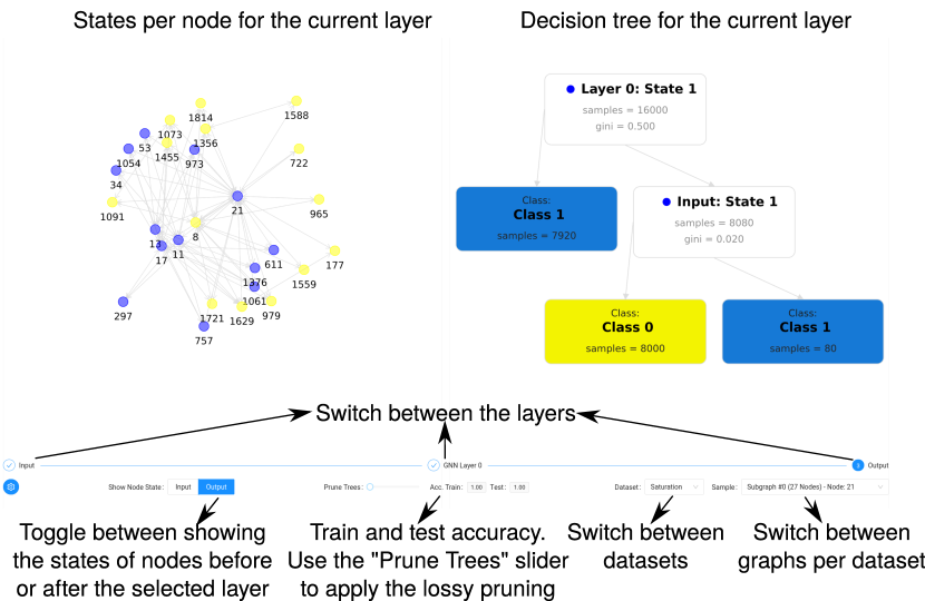
Figure 8: Initial page for the web tool. We can see the decision trees for DT+GNN per dataset and which node for a graph is in what state. We can switch layers, graphs and datasets. We can also see the test accuracy for the current setting and choose an amount of lossy pruning. with the slider.

A example instance of the tool is deployed and available via Netlify and can be accessed under the link https://interpretable-gnn.netlify.app/. The supplementary material also contains code to host the interface yourself, in case you want to try variations of DT+GNN. In the backend, we use PyTorch [Paszke et al., 2019] and PyTorch Geometric [Fey and Lenssen, 2019] to train DT+GNN and SKLearn[Pedregosa et al., 2011] to train decision trees.

The tool is built with React, in particular the Ant Design library. We visualize graphs with the Graphin library. The interface is a single page that will look similar to Figure 8.

The largest part of the interface is taken by two different panels at the top. In the right panel, you can see the decision tree for the currently selected layer. The trees use the three branching options from Figure 4. In the interface, evaluating the branching to true means taking the left path (this is opposite to Figure 4, which we will flip). In the left panel, you can see an example graph and which nodes end up in which state after this layer (in the bottom left you can toggle to see the input states instead). This panel does not show the full graph (most graphs in the datasets are prohibitively large) but an excerpt around an interesting region. Directly below these two graphics, you have the option to switch between layers by clicking on the respective bubble.

In the bottom right, you can switch to a different graph in the same dataset or to a different dataset. In the centre, you can see the accuracy of DT+GNN with the displayed layers. The slider allows to apply the lossy pruning from Section 3.3 and the accuracy values update to the selected pruning level.

The interface also allows us to examine a single node more closely by clicking on it (see Figure 9; here we clicked the blue node on the very right). Selecting reveals two things: In the graph panel, you can see the explanation scores from Section 3.4 for this node in this layer. In the tree panel, you can see the decision path in the tree for this node. This is particularly helpful if multiple leaves in the tree would lead to the same output state as in this example.

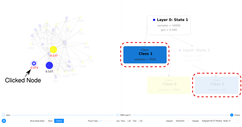
Figure 9: Interface when clicking on a node for closer examination. We can see node-level importance scores for this node on the left and the taken decision path on the right. Two paths end in the blue state, shown by the red boxes. The path the node takes is highlighted, the other path is blurred out.

Appendix B Datasets

B.1 Synthetic Datasets

• Infection Faber et al. [2021] is a synthetic node classification dataset. This dataset consists of randomly generated directed graphs, where each node can be healthy or infected. The classification task predicts the length of the shortest directed path from an infected node.

• Negative Evidence Faber et al. [2021] is a synthetic node classification dataset. A random graph with ten red nodes, ten blue nodes, and 1980 white nodes is created. The task is to determine whether the white nodes have more red or blue neighbours.

• BA Shapes Ying et al. [2019] is a synthetic node classification dataset. Each graph contains a Barabasi-Albert (BA) base graph and several house-like motifs attached to random nodes of the base graph. The node labels are determined by the node’s position in the house motif or base graph.

• Tree Cycle Ying et al. [2019] is a synthetic node classification dataset. Each graph contains an 8-level balanced binary tree and a six-node cycle motif attached to random nodes of the tree. The classification task predicts whether the nodes are part of the motif or tree.

• Tree Grid Ying et al. [2019] is a synthetic node classification dataset. Each graph contains an 8-level balanced binary tree and a 3-by-3 grid motif attached to random nodes of the tree. The classification task predicts whether the nodes are part of the motif or the tree.

• BA 2Motifs Luo et al. [2020] is a synthetic graph classification dataset. Barabasi-Albert graphs are used as the base graph. Half of the graphs have a house-like motif attached to a random node, and the other half have a five-node cycle. The prediction task is to classify each graph, whether it contains a house or a cycle.

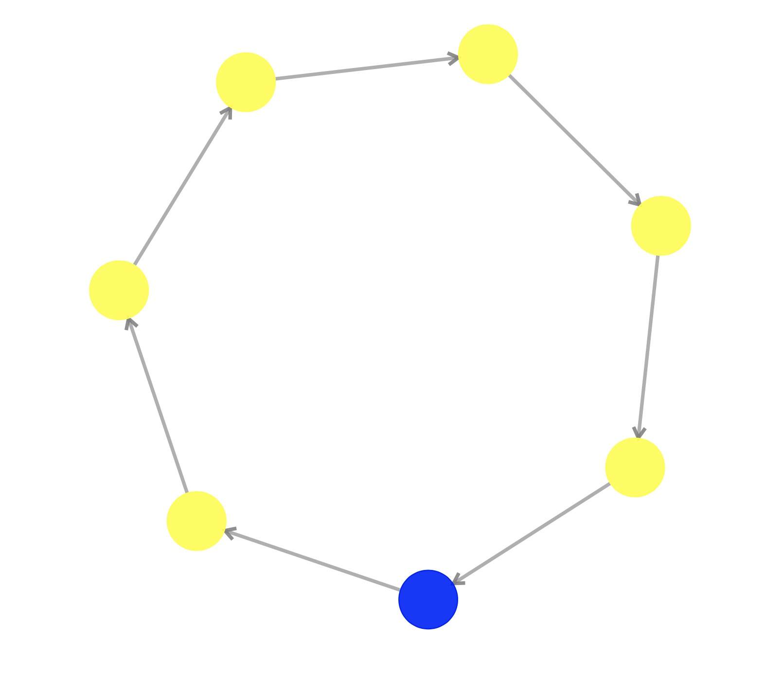
(a)

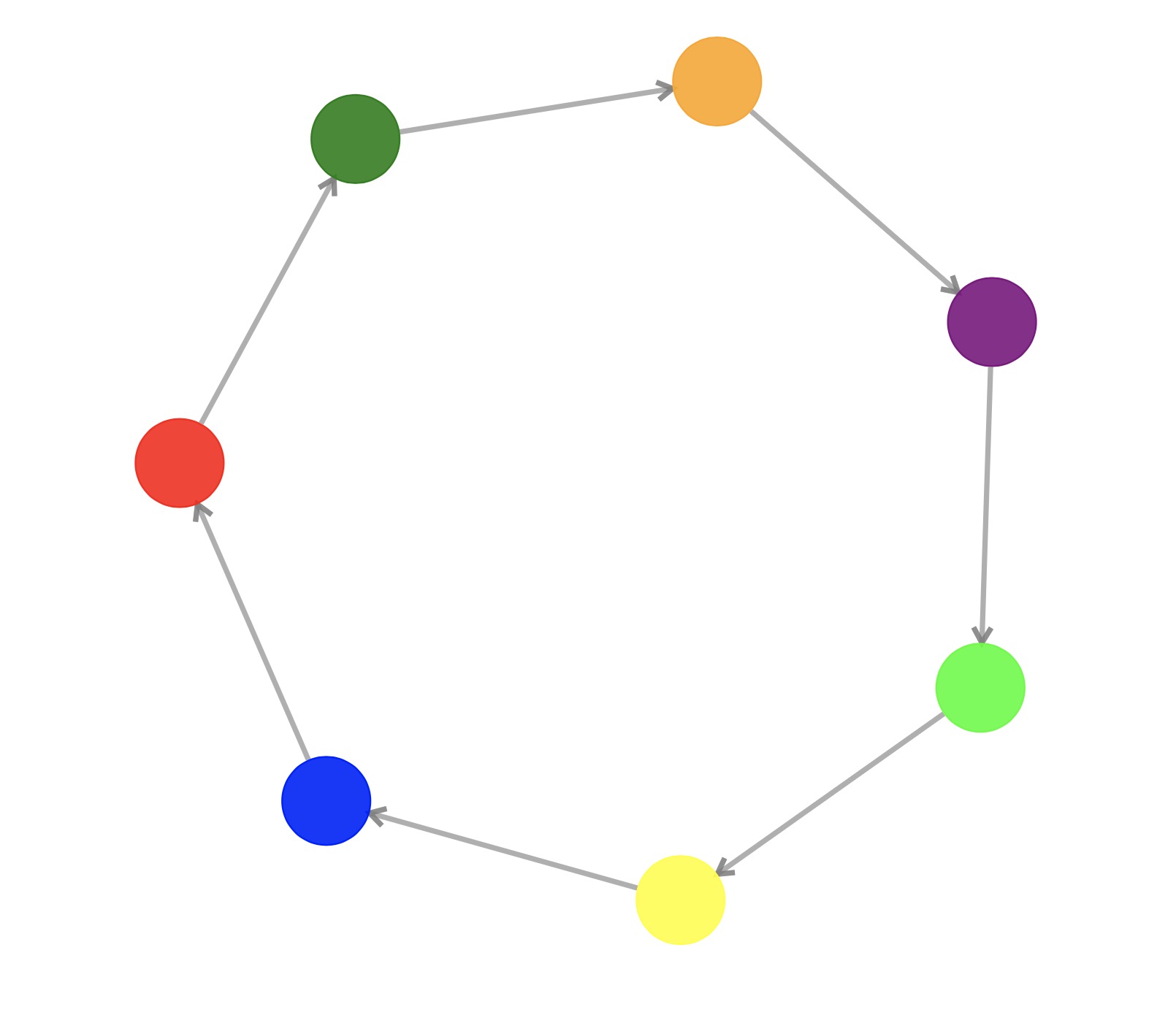
(b)

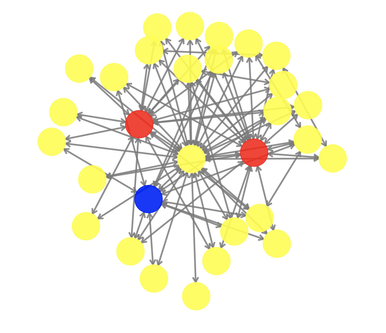
(c)

(d)

(e)

(f)

(g)

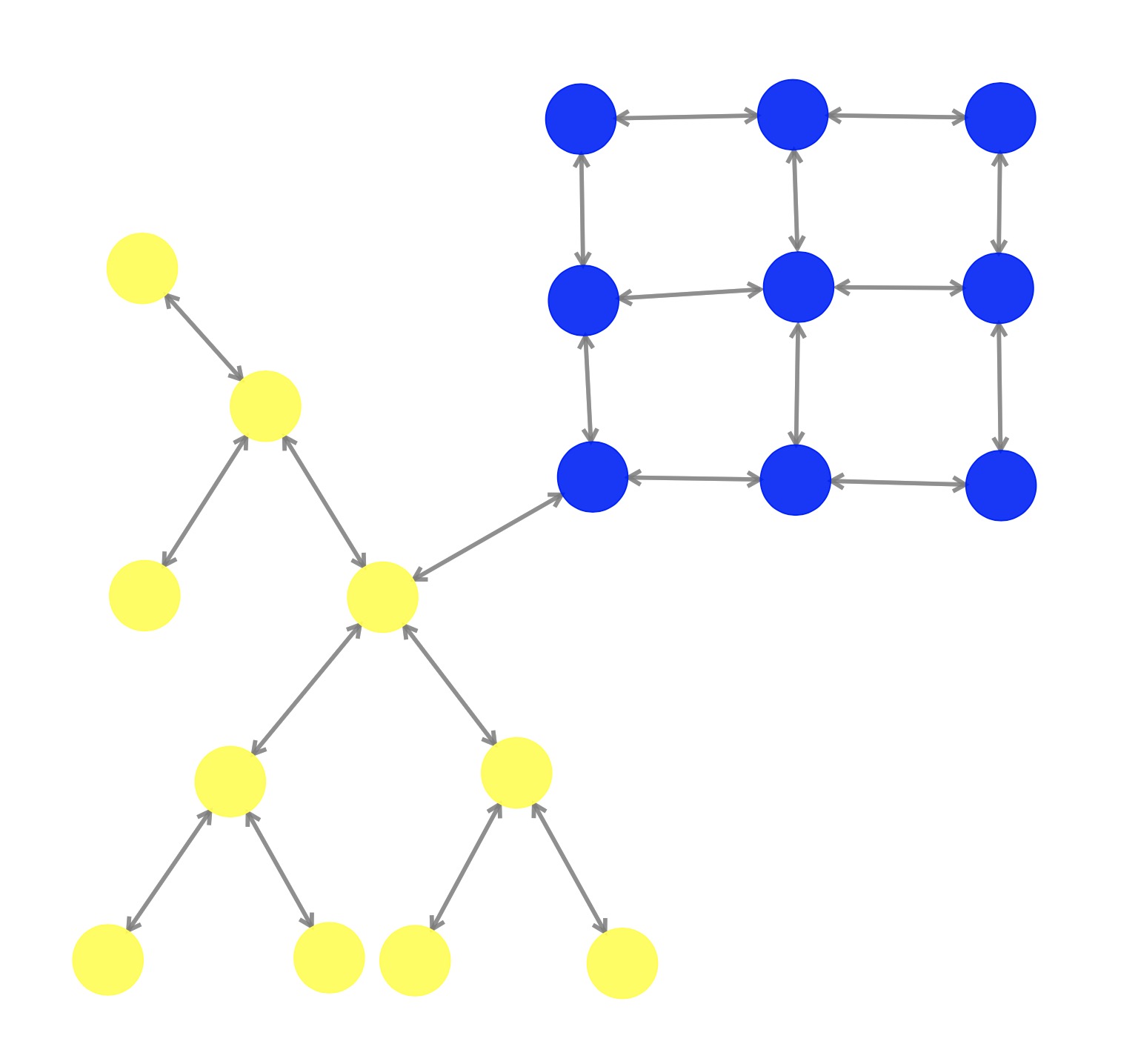
(h)

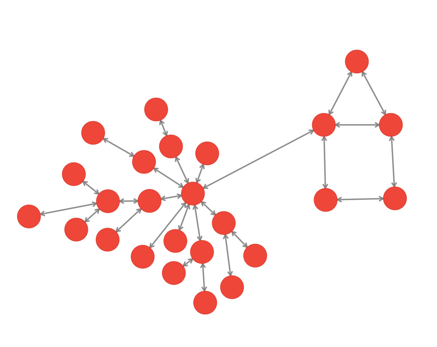
(i)

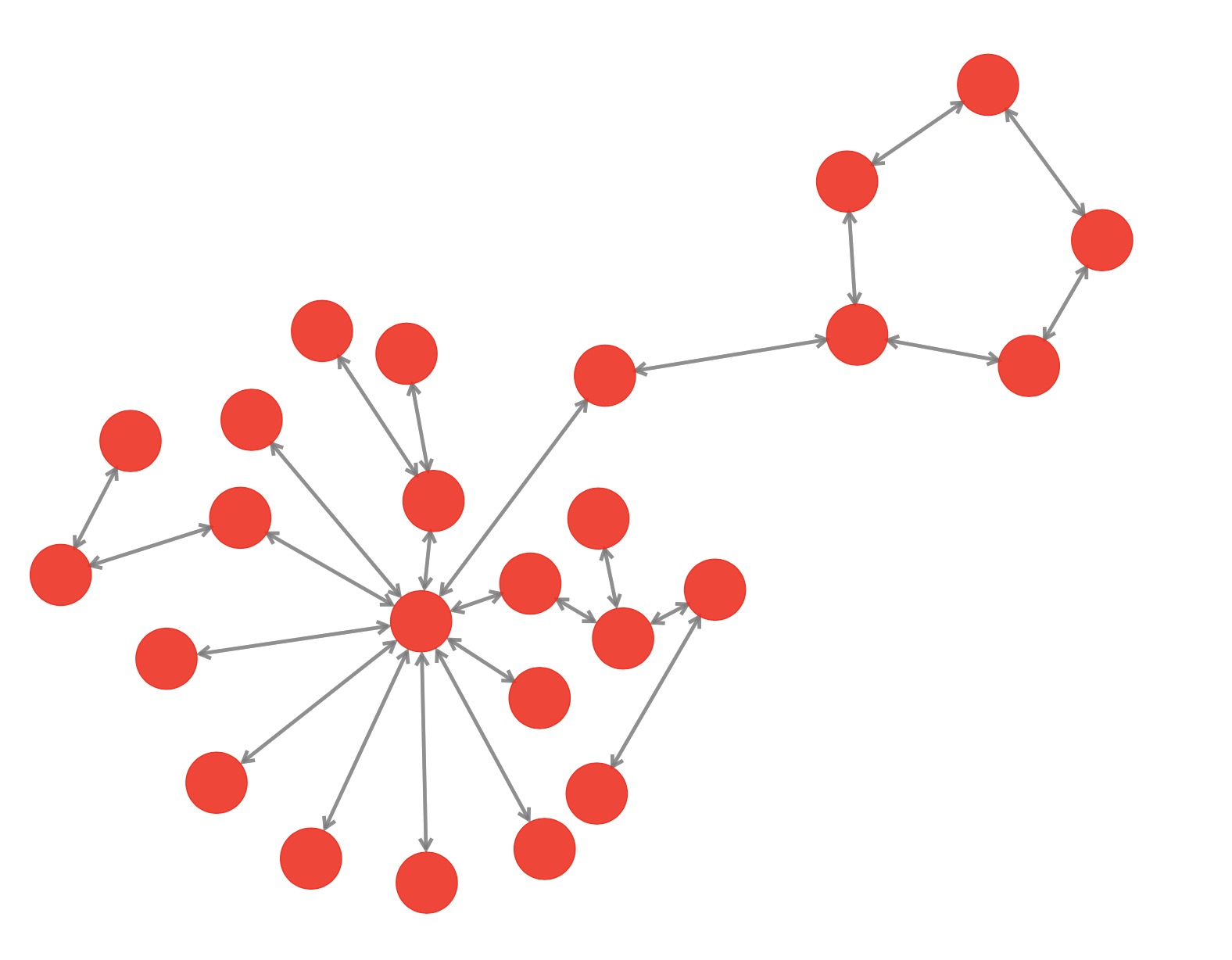
(j)

Figure 10: Synthetic Benchmarks - Example Graphs

Dataset	Graphs	Classes	Avg. Nodes	Avg. Edges	Features
Infection	1	7	1000	3973	2
Negative Evidence	1	2	2000	102394	3
BA Shapes	1	4	700	4110	0
Tree Cycle	1	2	871	1942	0
Tree Grid	1	2	1231	3130	0
BA 2Motifs	1000	2	25	50.96	0

Table 3: Statistics of Synthetic Datasets

B.2 Real-World Datasets

• MUTAG Debnath et al. [1991] is a molecule graph classification dataset. Each graph represents a nitroaromatic compound, and the goal is to predict its mutagenicity in Salmonella typhimurium. Mutagenicity is the ability of a compound to change the genetic material permanently, usually DNA, in an organism and therefore increase the frequency of mutations. The nodes in the graph represent atoms and are labeled by atom type. The edges represent bonds between atoms.

• Mutagenicity Kazius et al. [2005] is a molecule graph classification dataset. Each graph represents the chemical compound of a drug, and the goal is to predict its mutagenicity. The nodes in the graph represent atoms and are labeled by atom type. The edges represent bonds between atoms.

• BBBP Wu et al. [2017b] is a molecule graph classification dataset. Each graph represents the chemical compound of a drug, and the goal is to predict its blood-brain barrier permeability. The nodes in the graph represent atoms and are labeled by atom type. The edges represent bonds between atoms.

• PROTEINS Borgwardt et al. [2005] is a protein graph classification dataset. Each graph represents a protein that is classified as an enzyme or not and enzyme. Nodes represent the amino acids, and an edge connects two nodes if they are less than 6 Angstroms apart.

• REDDIT BINARY Borgwardt et al. [2005] is a social graph classification dataset. Each graph represents the comment thread of a post on a subreddit. Nodes in the graph represent users, and there is an edge between users if one responded to at least one of the other’s comments. A graph is labeled according to whether it belongs to a question/answer-based or a discussion-based subreddit.

• IMDB BINARY Borgwardt et al. [2005] is a social graph classification dataset. Each graph represents the ego network of an actor/actress. In each graph, nodes represent actors/actresses, and there is an edge between them if they appear in the same film. A graph is labeled according to whether the actor/actress belongs to the Action or Romance genre.

• COLLAB Borgwardt et al. [2005] is a social graph classification dataset. A graph represents a researcher’s ego network. The researcher and their collaborators are nodes, and an edge indicates collaboration between two researchers. A graph is labeled according to whether the researcher belongs to the field of high-energy physics, condensed matter physics, or astrophysics.

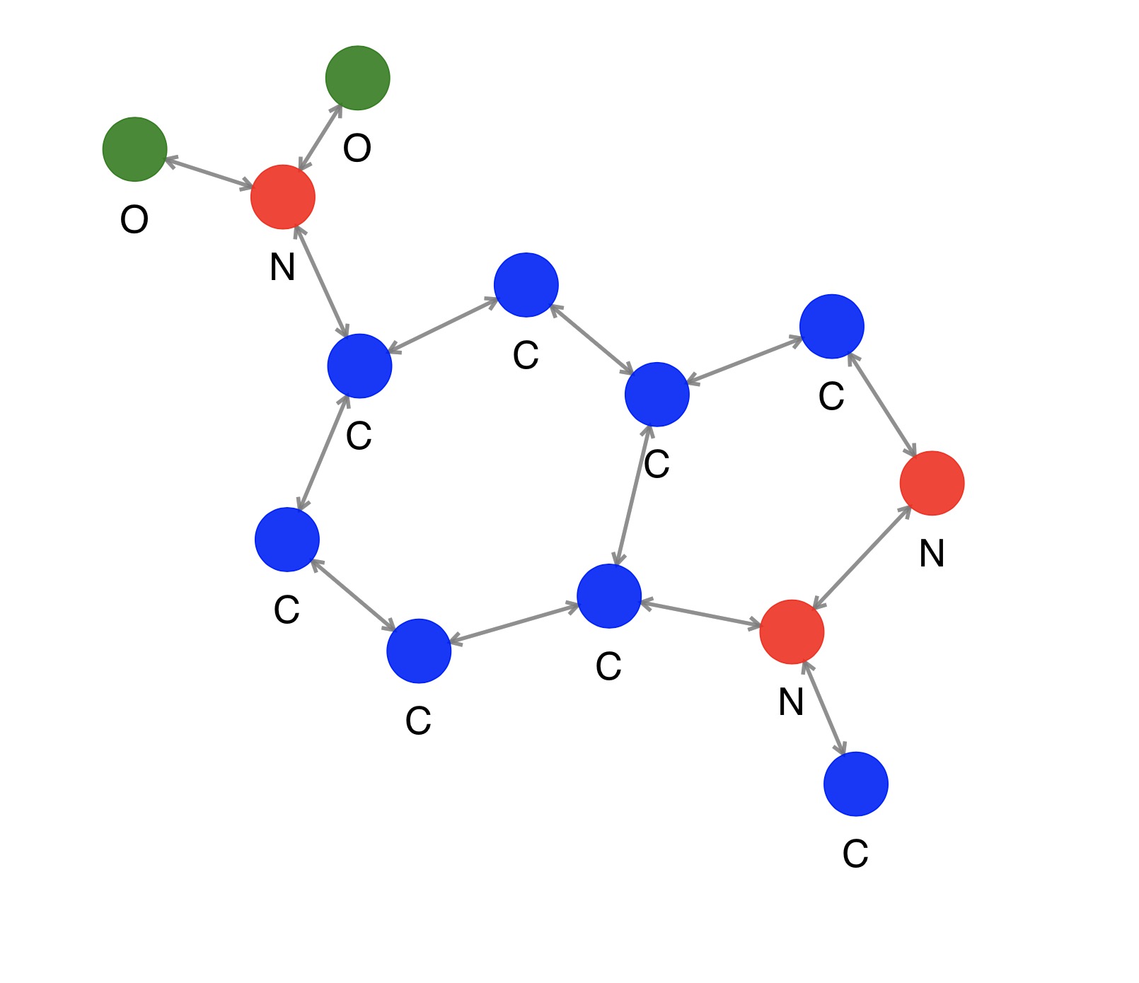
(a)

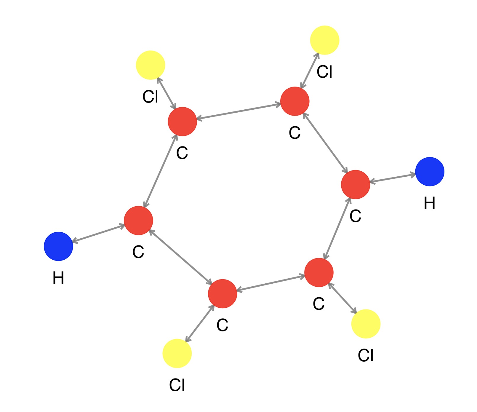
(b)

(c)

(d)

(e)

(f)

(g)

Figure 11: Real-world benchmarks - Example graphs

Dataset	Graphs	Classes	Avg. Nodes	Avg. Edges	Features
MUTAG	188	2	17.93	39.59	7
Mutagenicity	4337	2	30.32	61.54	14
BBBP	2039	2	24.06	51.91	9
PROTEINS	1113	2	39.06	145.63	3
REDDIT BINARY	2000	2	429.63	995.51	0
IMDB BINARY	1000	2	19.77	193.06	0
COLLAB	5000	3	74.49	4914.43	0

Table 4: Statistics of Real-World Datasets

Appendix C More Qualitative Experiments

C.1 BA-Shapes

We first want to discuss the approach learned by DT+GNNs to solving the BA-Shapes dataset [Ying et al., 2019]. The goal is to identify the nodes in a house (bottom, middle, top) versus the underlying base graph. The base graph is more densely connected than the house so DT+GNN first identifies nodes with at most degree $3$ (Figure 12(a)). This identifies almost every node in the house but the ones that connect the house to the graph. These nodes are found in the next step (12(c)). From here, DT+GNN needs to map the nodes in the house to their respective positions. It starts by finding the two middle nodes with a degree larger than $2$ (Figure 12(e)). Last, it can distinguish the top from the bottom nodes, since the top has no other degree $2$ neighbor (Figure 12(g)).

(a)

(b)

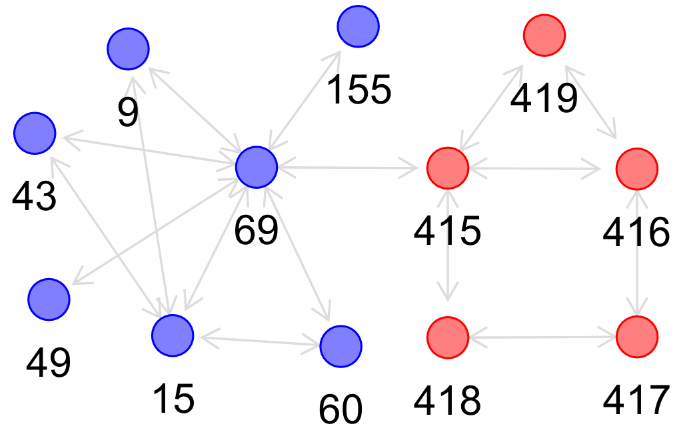
(c)

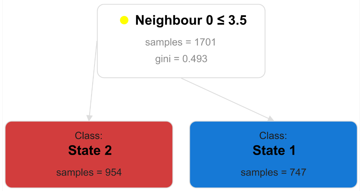
(d)

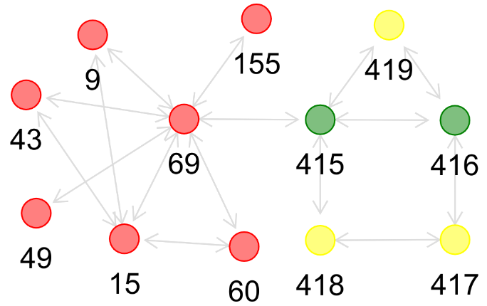
(e)

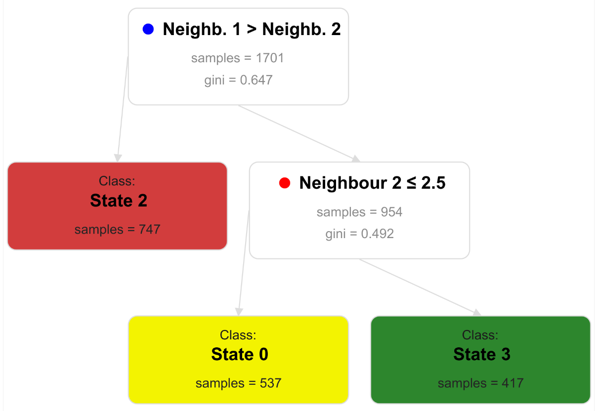
(f)

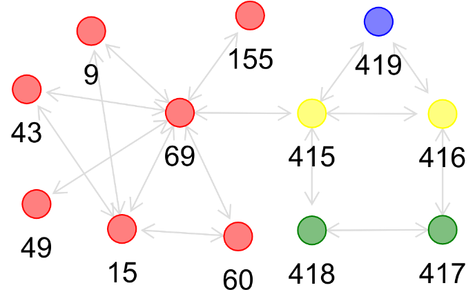
(g)

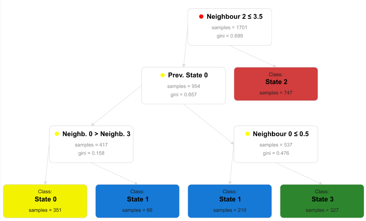
(h)

Figure 12: DT+GNN solves an instance of the BA-shapes dataset. Figures (a), (c), (e), and (g) show the different states of nodes through different layers, and the other plots (b), (d), (f), and (h) show the respective decision trees. Numbers denote node IDs. (a)-(d) First, DT+GNN gets an idea of where the house is by finding low-degree nodes. (e) and (f) Inside the house, DT+GNN finds the nodes with a degree of $2$; the nodes with a higher degree form the center. (g) and (h) The lonely node is the top of the house while the two connected degree $2$ nodes are the bottom.

C.2 Tree-Grid

The Tree-Grid [Ying et al., 2019] dataset is similar to the Tree-Cycles dataset we discussed in the main body of the paper. The base graph is a balanced binary tree to which we append $3\times 3$ grids. As in the Tree-Cycles example, a GNN does not need to see the whole grid to make a prediction.

Because the base graph is a balanced binary tree, only the root node and corner nodes in the grid have a degree of $2$. DT+GNN first finds the corner nodes (Figure 13(a)). From there, DT+GNN can incrementally build the grid by adding the neighboring nodes, finishing after two sets of expansion (Figures 13(b) and 13(c)). Similar to the Tree-Cycle example, we do not need to read the whole grid structure. Therefore, it would be wrong to expect an explanation method to highlight all of the grid. For example, DT+GNN’s explanation does not use the node in the $4-$hop neighborhood in the opposite corner in the explanation (Figure 13(d)) since it did not look that far.

(a)

(b)

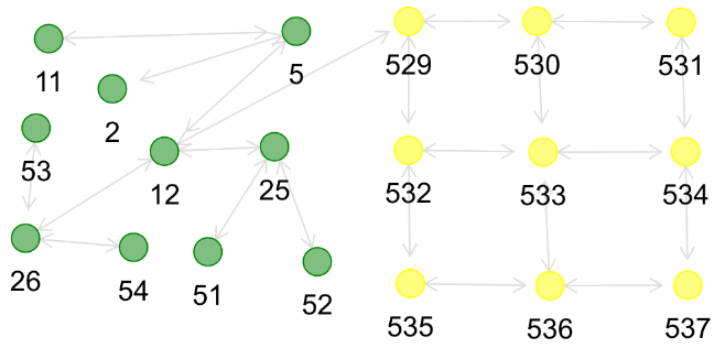
(c)

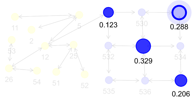
(d)

Figure 13: DT+GNN solves an instance of the Tree-Grid dataset. Figures (a)-(c) show the progression of node states for the first three layers. Numbers denote node IDs. (a) DT+GNN finds nodes of degree $2$ in the first layer, the corners of the grid. (b) DT+GNN finds the neighbors of the corner nodes. (c) DT+GNN finds the nodes next to the previous nodes — completing the grid. (d) This plot shows the explanation scores for the top-right node. Explanations are the $2-$distance neighborhood. Importantly, the bottom-left node in the grid was never seen by the top-right node — rightfully it is not part of the explanation.

C.3 MUTAG

As discussed in the main body, the presence of $NO_{2}$ groups in MUTAG [Debnath et al., 1991] is not informative for mutagenicity since all graphs have such a group. Instead, DT+GNN counts the nodes that have $3$ neighbors of a degree of $2$ or more (Figure 14(b)). Therefore, DT+GNN is looking for atoms that are not connected to $O$ (Figure 14(a)). If a graph has at least $4$ such nodes, it is mutagenic (Figure 14(c)).

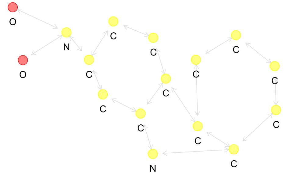
(a)

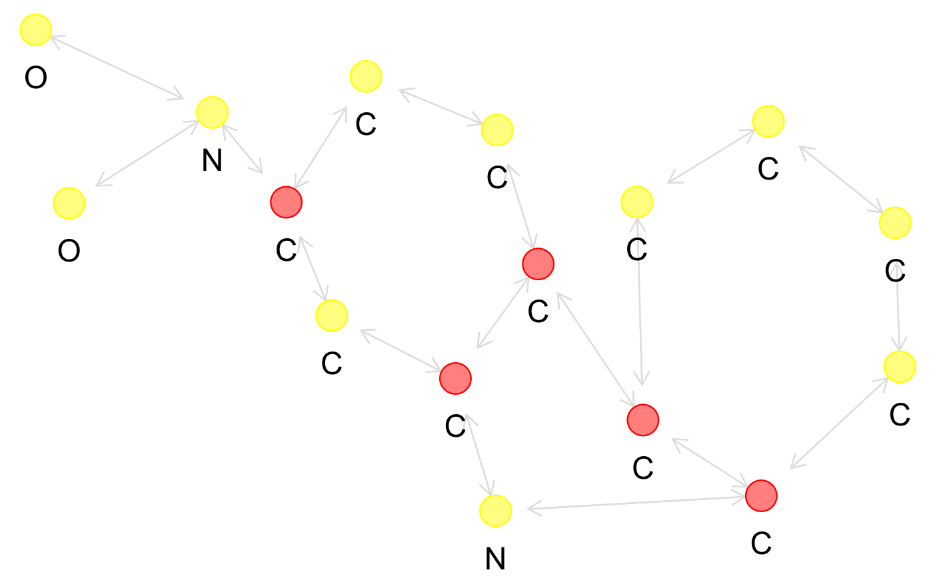
(b)

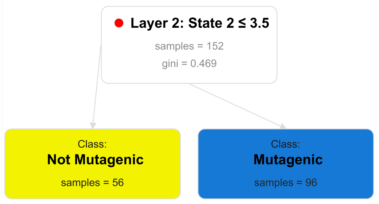
(c)

Figure 14: DT+GNN solves an instance of the MUTAG dataset. (a) and (b) show the learned node states for the first two layers. Numbers denote node IDs. (a) DT+GNN finds $O$ atoms by a degree count (b) DT+GNN finds nodes that have $3$ connections but not to $O$ atoms. (c) shows the final decoder layer. If there are $4$ or red nodes from the second layer (see (b)), the graph is mutagenic.

C.4 REDDIT-BINARY

This dataset [Borgwardt et al., 2005] consists of unattributed graphs that represent a thread in a subreddit. Nodes represent Reddit users; edges are between two users where one commented on another. Depending on the subreddit, the graph has the label “Discussion” or “Q&A”. Ying et al. [2019] analyzed this dataset before: characteristic of “Q&A” graphs are the high-degree nodes that represent the users answering questions. DT+GNN also finds these users in the first layer (Figure 15(a)). Interestingly, DT+GNN bases its prediction on the neighbors of these central nodes. It splits these neighbors into those that interacted with at least $2$ other nodes and those who do not (Figure 15(b)). Only if at least $25$ neighbors were interactive, DT+GNN considers the graph a “Q&A” graph (Figure 15(c)).

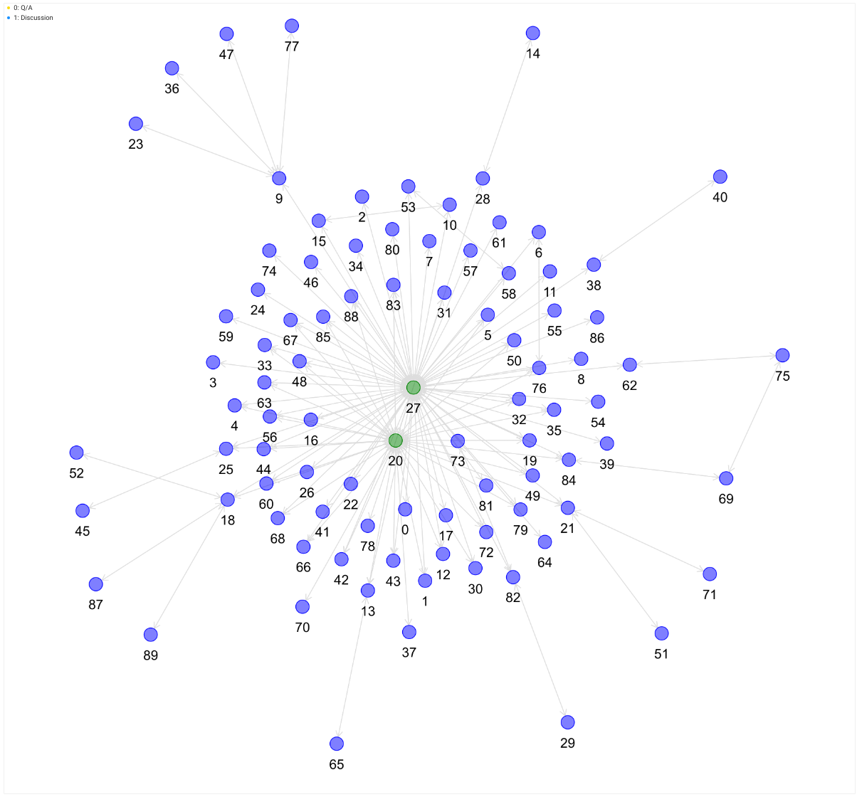
(a)

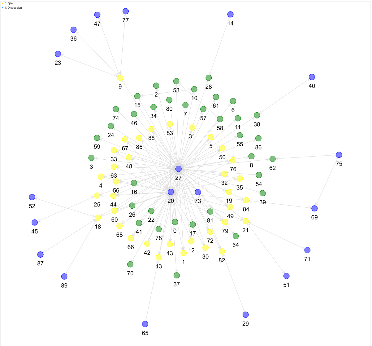
(b)

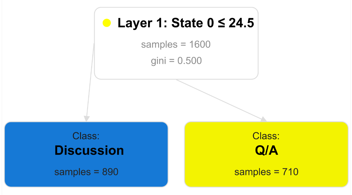
(c)

Figure 15: DT+GNN solves a “Q&A” instance of the REDDIT-BINARY dataset. (a) and (b) show the learned node states for the first two layers. Numbers denote node IDs. (a) DT+GNN finds the high-degree nodes answering questions. (b) DT+GNN then finds the neighbors of the central nodes that also interact with other nodes (c) shows the decoder decision tree. Since there are $25$ or more such interactive nodes, DT+GNN considers the graph “Q&A”.

References

- Agarwal et al. [2022] C. Agarwal, M. Zitnik, and H. Lakkaraju. Probing gnn explainers: A rigorous theoretical and empirical analysis of gnn explanation methods. In International Conference on Artificial Intelligence and Statistics (AISTATS), virtual, 2022.
- Baldassarre and Azizpour [2019] F. Baldassarre and H. Azizpour. Explainability techniques for graph convolutional networks. In International Conference on Machine Learning (ICML) Workshop on Learning and Reasoning with Graph-Structured Representations, 2019.
- Bian et al. [2020] T. Bian, X. Xiao, T. Xu, P. Zhao, W. Huang, Y. Rong, and J. Huang. Rumor detection on social media with bi-directional graph convolutional networks. In AAAI conference on artificial intelligence (AAAI), 2020.
- Borgwardt et al. [2005] K. M. Borgwardt, C. S. Ong, S. Schonauer, S. V. N. Vishwanathan, A. J. Smola, and H.-P. Kriegel. Protein function prediction via graph kernels. Bioinformatics, 2005.
- Boz [2002] O. Boz. Extracting decision trees from trained neural networks. In ACM SIGKDD international conference on Knowledge discovery and data mining (KDD), 2002.
- Cai and Wang [2018] C. Cai and Y. Wang. A simple yet effective baseline for non-attributed graph classification. In International Conference on Learning Representations (ICLR) Workshop on Representation Learning on Graphs and Manifolds, 2018.
- Chen et al. [2019] T. Chen, S. Bian, and Y. Sun. Are Powerful Graph Neural Nets Necessary? A Dissection on Graph Classification. ArXiv, 2019.
- Dai and Wang [2021] E. Dai and S. Wang. Towards Self-Explainable Graph Neural Network. In ACM International Conference on Information & Knowledge Management (CIKM), 2021.
- Dancey et al. [2004] D. Dancey, D. Mclean, and Z. Bandar. Decision Tree Extraction from Trained Neural Networks. In International Florida Artificial Intelligence Research Society Conference (FLAIRS), 2004.
- Debnath et al. [1991] A. K. Debnath, R. L. Lopez de Compadre, G. Debnath, A. J. Shusterman, and C. Hansch. Structure-activity relationship of mutagenic aromatic and heteroaromatic nitro compounds. Correlation with molecular orbital energies and hydrophobicity. Journal of Medicinal Chemistry, 1991.
- Duval and Malliaros [2021] A. Duval and F. D. Malliaros. Graphsvx: Shapley value explanations for graph neural networks. In Joint European Conference on Machine Learning and Principles and Practice of Knowledge Discovery in Databases (ECML PKDD), 2021.
- Emek and Wattenhofer [2013] Y. Emek and R. Wattenhofer. Stone age distributed computing. In ACM Symposium on Principles of distributed computing (PODC), 2013.
- Errica et al. [2020] F. Errica, M. Podda, D. Bacciu, and A. Micheli. A fair comparison of graph neural networks for graph classification. In International Conference on Learning Representations (ICLR 2020), 2020.
- Faber et al. [2020] L. Faber, A. K. Moghaddam, and R. Wattenhofer. Contrastive Graph Neural Network Explanation. In Proceedings of the 37th International Conference on Machine Learning (ICML) Workshop on Graph Representation Learning and Beyond (GRL+), 2020.
- Faber et al. [2021] L. Faber, A. K. Moghaddam, and R. Wattenhofer. When Comparing to Ground Truth is Wrong. In ACM SIGKDD Conference on Knowledge Discovery & Data Mining (KDD), 2021.
- Fey and Lenssen [2019] M. Fey and J. E. Lenssen. Fast graph representation learning with PyTorch Geometric. In ICLR Workshop on Representation Learning on Graphs and Manifolds, 2019.
- Gilmer et al. [2017] J. Gilmer, S. S. Schoenholz, P. F. Riley, O. Vinyals, and G. E. Dahl. Neural Message Passing for Quantum Chemistry. In International Conference on Machine Learning (ICML), 2017.
- Gorishniy et al. [2021] Y. Gorishniy, I. Rubachev, V. Khrulkov, and A. Babenko. Revisiting deep learning models for tabular data. Advances in Neural Information Processing Systems, 2021.
- Himmelhuber et al. [2021] A. Himmelhuber, M. Joblin, M. Ringsquandl, and T. Runkler. Demystifying Graph Neural Network Explanations. In Joint European Conference on Machine Learning and Principles and Practice of Knowledge Discovery in Databases (ECML PKDD), 2021.
- Hu et al. [2020] W. Hu, M. Fey, M. Zitnik, Y. Dong, H. Ren, B. Liu, M. Catasta, and J. Leskovec. Open Graph Benchmark: Datasets for Machine Learning on Graphs. ArXiv, 2020.
- Huang et al. [2020] Q. Huang, M. Yamada, Y. Tian, D. Singh, D. Yin, and Y. Chang. GraphLIME: Local Interpretable Model Explanations for Graph Neural Networks. ArXiv, 2020.
- Huang et al. [2021] Q. Huang, H. He, A. Singh, S.-N. Lim, and A. R. Benson. Combining Label Propagation and Simple Models Out-performs Graph Neural Networks. International Conference on Learning Representations (ICLR), 2021.
- Ioffe and Szegedy [2015] S. Ioffe and C. Szegedy. Batch normalization: Accelerating deep network training by reducing internal covariate shift. In International Conference on Machine Learning (ICML), 2015.
- Jang et al. [2016] E. Jang, S. Gu, and B. Poole. Categorical Reparameterization with Gumbel-Softmax. International Conference on Learning Representations (ICLR), 2016.
- Jumper et al. [2021] J. Jumper, R. Evans, A. Pritzel, T. Green, M. Figurnov, O. Ronneberger, K. Tunyasuvunakool, R. Bates, A. Žídek, A. Potapenko, et al. Highly accurate protein structure prediction with alphafold. Nature, 2021.
- Kazius et al. [2005] J. Kazius, R. McGuire, and R. Bursi. Derivation and validation of toxicophores for mutagenicity prediction. Journal of medicinal chemistry, 2005.
- Kontschieder et al. [2015] P. Kontschieder, M. Fiterau, A. Criminisi, and S. R. Bulo. Deep neural decision forests. In IEEE International Conference on Computer Vision (CVPR), 2015.
- Krishnan et al. [1999] R. Krishnan, G. Sivakumar, and P. Bhattacharya. Extracting decision trees from trained neural networks. Pattern Recognition, 1999.
- Loukas [2020] A. Loukas. What graph neural networks cannot learn: depth vs width. In International Conference on Learning Representations (ICLR), 2020.
- Lundberg et al. [2018] S. M. Lundberg, G. G. Erion, and S.-I. Lee. Consistent Individualized Feature Attribution for Tree Ensembles. ArXiv, 2018.
- Luo et al. [2020] D. Luo, W. Cheng, D. Xu, W. Yu, B. Zong, H. Chen, and X. Zhang. Parameterized explainer for graph neural network. In Conference on Neural Information Processing Systems (NeurIPS), 2020.
- Maddison et al. [2016] C. J. Maddison, A. Mnih, and Y. W. Teh. The Concrete Distribution: A Continuous Relaxation of Discrete Random Variables. In International Conference on Learning Representations (ICLR), 2016.
- Nair and Hinton [2010] V. Nair and G. E. Hinton. Rectified linear units improve restricted boltzmann machines. In International Conference on Machine Learning (ICML), 2010.
- Paszke et al. [2019] A. Paszke, S. Gross, F. Massa, A. Lerer, J. Bradbury, G. Chanan, T. Killeen, Z. Lin, N. Gimelshein, L. Antiga, A. Desmaison, A. Kopf, E. Yang, Z. DeVito, M. Raison, A. Tejani, S. Chilamkurthy, B. Steiner, L. Fang, J. Bai, and S. Chintala. Pytorch: An imperative style, high-performance deep learning library. In Conference on Neural Information Processing Systems (NeurIPS). 2019.
- Pedregosa et al. [2011] F. Pedregosa, G. Varoquaux, A. Gramfort, V. Michel, B. Thirion, O. Grisel, M. Blondel, P. Prettenhofer, R. Weiss, V. Dubourg, J. Vanderplas, A. Passos, D. Cournapeau, M. Brucher, M. Perrot, and E. Duchesnay. Scikit-learn: Machine learning in Python. Journal of Machine Learning Research, 2011.
- Peleg [2000] D. Peleg. Distributed computing: a locality-sensitive approach. SIAM, 2000.
- Pope et al. [2019] P. E. Pope, S. Kolouri, M. Rostami, C. E. Martin, and H. Hoffmann. Explainability methods for graph convolutional neural networks. In IEEE Conference on Computer Vision and Pattern Recognition (CVPR), 2019.
- Quinlan [1987] J. Quinlan. Simplifying decision trees. International Journal of Man-Machine Studies, 1987.
- Ribeiro et al. [2016] M. T. Ribeiro, S. Singh, and C. Guestrin. " why should i trust you?" explaining the predictions of any classifier. In ACM SIGKDD International Conference on Knowledge Discovery and Data Mining (KDD), 2016.
- Royden and Fitzpatrick [1988] H. L. Royden and P. Fitzpatrick. Real analysis. Macmillan New York, 1988.
- Sanchez-Lengeling et al. [2020] B. Sanchez-Lengeling, J. Wei, B. Lee, E. Reif, P. Wang, W. W. Qian, K. McCloskey, L. Colwell, and A. Wiltschko. Evaluating attribution for graph neural networks. In Conference on Neural Information Processing Systems (NeurIPS), 2020.
- Schaaf et al. [2019] N. Schaaf, M. F. Huber, and J. Maucher. Enhancing Decision Tree based Interpretation of Deep Neural Networks through L1-Orthogonal Regularization. 2019 18th IEEE International Conference On Machine Learning And Applications (ICMLA), 2019.
- Schlichtkrull et al. [2021] M. S. Schlichtkrull, N. D. Cao, and I. Titov. Interpreting graph neural networks for NLP with differentiable edge masking. In International Conference on Learning Representations (ICLR), 2021.
- Selvaraju et al. [2017] R. R. Selvaraju, M. Cogswell, A. Das, R. Vedantam, D. Parikh, and D. Batra. Grad-cam: Visual explanations from deep networks via gradient-based localization. In IEEE International Conference on Computer Vision (CVPR), 2017.
- Sen et al. [2008] P. Sen, G. Namata, M. Bilgic, L. Getoor, B. Galligher, and T. Eliassi-Rad. Collective classification in network data. AI magazine, 2008.
- Shapley [1953] L. S. Shapley. 17. A Value for n-Person Games. Contributions to the Theory of Games, 1953.
- Vu and Thai [2020] M. Vu and M. T. Thai. Pgm-explainer: Probabilistic graphical model explanations for graph neural networks. In Conference on Neural Information Processing Systems (NeurIPS), 2020.
- Wang et al. [2019] S. Wang, T. Zhou, and J. A. Bilmes. Bias Also Matters: Bias Attribution for Deep Neural Network Explanation. In International Conference on Machine Learning (ICML), 2019.
- Wu et al. [2017a] M. Wu, M. C. Hughes, S. Parbhoo, M. Zazzi, V. Roth, and F. Doshi-Velez. Beyond Sparsity: Tree Regularization of Deep Models for Interpretability. In AAAI Conference on Artificial Intelligence (AAAI), 2017a.
- Wu et al. [2017b] Z. Wu, B. Ramsundar, E. N. Feinberg, J. Gomes, C. Geniesse, A. S. Pappu, K. Leswing, and V. Pande. MoleculeNet: A Benchmark for Molecular Machine Learning. Chemical Science, 2017b.
- Xu et al. [2019] K. Xu, S. Jegelka, W. Hu, and J. Leskovec. How Powerful are Graph Neural Networks? International Conference on Learning Representations (ICLR), 2019.
- Yang et al. [2020] S. Yang, Z. Zhang, J. Zhou, Y. Wang, W. Sun, X. Zhong, Y. Fang, Q. Yu, and Y. Qi. Financial risk analysis for smes with graph-based supply chain mining. In International Joint Conferences on Artificial Intelligence (IJCAI), 2020.
- Yang et al. [2018] Y. Yang, I. G. Morillo, and T. M. Hospedales. Deep Neural Decision Trees. ArXiv, 2018.
- Ying et al. [2019] R. Ying, D. Bourgeois, J. You, M. Zitnik, and J. Leskovec. GNNExplainer: Generating Explanations for Graph Neural Networks. In Conference on Neural Information Processing Systems (NeurIPS), 2019.
- Yuan et al. [2020] H. Yuan, H. Yu, S. Gui, and S. Ji. Explainability in Graph Neural Networks: A Taxonomic Survey. ArXiv, 2020.
- Yuan et al. [2021] H. Yuan, H. Yu, J. Wang, K. Li, and S. Ji. On Explainability of Graph Neural Networks via Subgraph Explorations. In International Conference on Machine Learning (ICML), 2021.
- Zhang et al. [2021] Z. Zhang, Q. Liu, H. Wang, C. Lu, and C. Lee. ProtGNN: Towards Self-Explaining Graph Neural Networks. In AAAI Conference on Artificial Intelligence (AAAI), 2021.