Flocking and concentration behavior for the stochastic Cucker-Smale system in a harmonic field

Abstract.

We consider the Cucker-Smale system with multiplicative noise in a harmonic potential field and investigate the effect of harmonic potential field. In the presence of external potential force, the system is expected to emerge into almost surely velocity flocking and spatial concentration, due to the alignment mechanism, confining harmonic potential field and multiplicative noise. By constructing a stochastic Lyapunov functional, we derive a sufficient condition for the almost surely flocking and concentration behavior for the stochastic particle model, and verify it numerically. Then, we discuss the flocking and concentration behavior for the mean field Vlasov-type kinetic model. Moreover, a rigorous analysis of the uniform mean-field limit estimate for the limit process from the stochastic model to the kinetic one is provided.

1. Introduction

Collective behaviors of particle-based systems have been widely studied in recent years. When systems have a finite number of particles, it is often argued that the microscopic approach is the appropriate one. The particle Cucker-Smale (C-S) model is one of many microscopic attempts to represent such phenomena. It was originally introduced by Cucker and Smale [4], and studied by many authors, for example, [5, 6, 11, 12] for the particle system with different communication kernels, [9] for the particle system with time delay, [1, 7, 13] for the particle system with different noises, [3] for the kinetic C-S model. However, in many realistic scenarios, particles driven by alignment are also subject to environment forces. Recently, [14] introduced the following C-S model with the convex potential force $U$:

$$\left\{\begin{aligned} &{\dot{x}}_{t}^{i}=v_{t}^{i},\quad t>0,\quad 1\leq i\leq N,\\ &{\dot{v}}_{t}^{i}=\frac{\kappa}{N}\sum_{j=1}^{N}\psi(|x_{t}^{j}-x_{t}^{i}|)(v_{t}^{j}-v_{t}^{i})-\nabla U(x_{t}^{i}).\end{aligned}\right.$$ (1.1)

In this paper, similar to the work studied in [7], we add the stochastic influences to the deterministic dynamical system (LABEL:CS) with the quadratic potential $U(x)=\frac{1}{2}x^{2}$, and consider the following stochastic system

$$\left\{\begin{aligned} &dx_{t}^{i}=v_{t}^{i}dt,\qquad t>0,\quad 1\leq i\leq N,\\ &dv_{t}^{i}=\frac{\kappa}{N}\sum_{j=1}^{N}\psi(|x_{t}^{j}-x_{t}^{i}|)(v_{t}^{j}-v_{t}^{i})dt-x_{t}^{i}dt+\sqrt{2\sigma}(v_{t}^{i}-v_{t}^{c})dW_{t}.\end{aligned}\right.$$ (1.2)

$(x_{t}^{i},v_{t}^{i})\in\mathbb{R}^{2d}$ denote the velocity and position of the $i$th agent. The noise $W_{t}$ is the same Brownian motion in all directions of $\mathbb{R}^{d}$. The diagonal diffusion matrix $\sqrt{2\sigma}(v_{t}^{i}-v_{t}^{c})$ tells us that “noise intensity” depends on the localization of the velocity in a simple way, here $\sigma$ is a positive constant. $\psi(|x_{t}^{j}-x_{t}^{i}|)$ is a communication weight function and satisfies the symmetry condition and translation invariance. $|\cdot|$ denotes the standard $\ell^{2}$-norm in $\mathbb{R}^{d}$.

When the number of particles $N$ is excessively large, it becomes increasingly difficult to follow the dynamics of each individual agent. Hence, instead of simulating the behavior of each individual agent, we would like to describe the kinetic collective behavior encoded by the density distribution whose evolution is governed by one sole mesoscopic partial differential equation. Applying the BBGKY hierarchy, one can derive the following corresponding kinetic model from (LABEL:SCS1):

$$\begin{split}&\partial_{t}f+v\cdot\nabla_{x}f+\nabla_{v}\cdot(L[f]f)-x\cdot\nabla_{v}f=\sigma\Delta_{v}(|v-v_{c}|^{2}f),\\ &L[f](x,v,t):=-\kappa\int_{\mathbb{R}^{2d}}\psi\left(|x-y|\right)\left(v-v_{\ast}\right)f(y,v_{\ast},t)dv_{\ast}dy,\quad x,v\in\mathbb{R}^{d},\ t>0,\\ \end{split}$$ (1.3)

subject to suitable initial configuration

$$\begin{split}&f(x,v,0)=f_{0}(x,v).\\ \end{split}$$ (1.4)

In this paper, we address the following question:

(Q):  With the confining harmonic potential, can we drive a sufficient condition to rigorously verify the formation of the velocity flocking and spatial concentration result both for the stochastic particle model (LABEL:SCS1) and related mean-field Vlasov-type kinetic model (1.3)?

We exploit the above question from both the analytic and numerical views. First we derive a sufficient framework leading to the formation of the almost surely flocking in velocity and spatial concentration due to the alignment mechanism, confining potential and multiplicative noise. Without the confining potential field, the authors proved the velocity flocking result by deriving a differential inequality system and solving a geometric Brownian motion equation for the velocity directly [1]. The result in their paper also implied that the multiplicative noise could give the strong flocking result, compared with the case of the additive noise. However, system (LABEL:SCS1) is coupled by the existence of confining harmonic field. We use the Lyapunov functional method and define a related differential operator to get the almost surely velocity flocking and spatial concentration result. By using Euler’s method, we verify the analytic results numerically.

Second, we study the long-time behavior for the related mean-field Vlasov-type kinetic model (1.3). We introduce a Lyapunov functional $\tilde{\mathcal{L}}[f]$ (see (3.5)), which is equivalent to the standard Lyapunov functional $\mathcal{L}[f]$( see (3.6)) measuring the position and velocity variances of the kinetic density function $f$. We exploit a sufficient condition for the flocking and concentration result for the mean-field Vlasov-type kinetic model (1.3). Due to the confining potential term, the standard Lyapunov functional is not enough to derive the Grönwall’s type inequality for it. Therefore we consider the equivalent functional containing the cross term $\int_{\mathbb{R}^{2d}}(x-x_{c})\cdot(v-v_{c})fdxdv$. We also address the existence of the classical solution for the kinetic model in a weighted Sobolev space.

Third, since we are dealing with the Vlasov-type kinetic equation corresponding to the stochastic particle C-S model with a harmonic potential field, we discuss the mean-field limit and provide the rigorous analysis for it. In [2], rigorous finite-in-time mean-field limit has been derived from the C-S particle system with additive noise to the corresponding C-S Vlasov-type equation. However, to get the uniform-in-time mean-field limit estimate for our model, we need to perform a more rigorous analysis, considering the coupling difficulty brought by the confining potential filed. We also utilize the detailed information of the McKean process, which was developed in [15]. Therefore, by making use of the flocking estimate for the limit process, we establish the proof of the uniform-in-time mean-field limit.

We introduce the following definition.

Definition 1.1.

The stochastic system has an asymptotic strong stochastic flocking in velocity and concentration in position if the position and velocity processes $\{x_{t}^{i},v_{t}^{i}\}$($i=1,\cdots,N$) satisfy the following condition: For $1\leq i,j\leq N$, the differences of all pairwise position and velocity processes go to zero asymptotically,

$$\lim_{t\to\infty}(|x_{t}^{i}-x_{t}^{j}|+|v_{t}^{i}-v_{t}^{j}|)=0,\quad a.s.$$

The rest of this paper is organized as follows. In Section 2, we study the velocity flocking and spatial concentration result for the stochastic particle model analytically and numerically. In Section 3, we present the well-posedness and long-time behavior of the kinetic C-S Vlasov-type equation. In Section 4, we prove the uniform-in-time mean-field limit from the stochastic particle C-S system to the kinetic C-S Vlasov-type equation.

2. Stochastic particle system

In this section, we study the velocity flocking and spatial concentration result for the stochastic particle model (LABEL:SCS1) analytically and numerically. We first introduce a macro-micro decomposition to decompose the system into two parts: one system describes the macroscopic dynamics and the other system describes the microscopic fluctuations.

2.1. A Macro-Micro decomposition

For the stochastic flocking estimate, we introduce macro (ensemble average) process

$$x_{t}^{c}=\frac{1}{N}\sum_{i=1}^{N}x_{t}^{i},\quad v_{t}^{c}=\frac{1}{N}\sum_{i=1}^{N}v_{t}^{i}$$

and micro (fluctuation) process

$$\hat{x}_{t}^{i}=x_{t}^{i}-x_{t}^{c},\quad\hat{v}_{t}^{i}=v_{t}^{i}-v_{t}^{c}.$$

Then $\sum\limits_{i=1}^{N}\hat{x}_{t}^{i}=\sum\limits_{i=1}^{N}\hat{v}_{t}^{i}=0$.

Averaging over $i$ in (LABEL:SCS1) gives the evolution of $(x_{t}^{c},v_{t}^{c})$:

$$\left\{\begin{split}&dx_{t}^{c}=v_{t}^{c}dt,\\ &dv_{t}^{c}=-x_{t}^{c}dt.\end{split}\right.$$ (2.1)

Given the deterministic initial configuration $(x^{c}_{0},v^{c}_{0})$, one can get the dynamics of the macroscopic variables $(x_{t}^{c},v_{t}^{c})$, which satisfy the harmonic oscillator motion as follows:

$$x^{c}_{t}=x^{c}_{0}\cos t+v^{c}_{0}\sin t,\quad v^{c}_{t}=v^{c}_{0}\cos t-x^{c}_{0}\sin t,\quad a.s.$$

Next, we subtract (2.1) from (LABEL:SCS1) to derive the evolution of perturbation $(\hat{x}_{t}^{i},\hat{v}_{t}^{i})$:

$$\left\{\begin{split}&d\hat{x}_{t}^{i}=\hat{v}_{t}^{i}dt,\\ &d\hat{v}_{t}^{i}=\frac{\kappa}{N}\sum_{j=1}^{N}\psi(|\hat{x}_{t}^{j}-\hat{x}_{t}^{i}|)(\hat{v}_{t}^{j}-\hat{v}_{t}^{i})dt-\hat{x}_{t}^{i}dt+\sqrt{2\sigma}\hat{v}_{t}^{i}dW_{t}.\end{split}\right.$$ (2.2)

In the next subsection, we will show that the stochastic system (LABEL:SCS1) flocks in the sense of Definition 1.1. Since

$$\lim_{t\to\infty}(|x_{t}^{i}-x_{t}^{j}|+|v_{t}^{i}-v_{t}^{j}|)=\lim_{t\to\infty}(|\hat{x}_{t}^{i}-\hat{x}_{t}^{j}|+|\hat{v}_{t}^{i}-\hat{v}_{t}^{j}|),$$

it is sufficient to show that the flocking and concentration occur in the microscopic system (LABEL:micro).

2.2. The dynamics of the microscopic system

In this subsection, we consider the dynamics of the microscopic variable given by system (LABEL:micro). We rewrite it without the hat notation:

$$\left\{\begin{aligned} &dx_{t}^{i}=v_{t}^{i}dt,\quad t>0,\\ &dv_{t}^{i}=\frac{\kappa}{N}\sum_{j=1}^{N}\psi(|x_{t}^{j}-x_{t}^{i}|)(v_{t}^{j}-v_{t}^{i})dt-x_{t}^{i}dt+\sqrt{2\sigma}v_{t}^{i}dW(t),\\ &\sum\limits_{i=1}^{N}x_{t}^{i}=0,\quad\sum\limits_{i=1}^{N}v_{t}^{i}=0.\end{aligned}\right.$$ (2.3)

We analyze this radially symmetric communication weight function with multiplicative noise system following the Lyapunov functional method in book [10]. Generally speaking, to deal with the following general SDE:

$$d\mathbf{x}(t)=f(\mathbf{x}(t),t)dt+g(\mathbf{x}(t),t)dW(t),\quad\mathbf{x}=(x_{1},x_{2},\cdots,x_{n}),$$ (2.4)

one could define the differential operator $\mathscr{L}$ associated with equation (2.4) by

$$\mathscr{L}:=\frac{\partial}{\partial t}+\sum\limits_{i=1}^{N}f_{i}(\mathbf{x},t)\frac{\partial}{\partial x_{i}}+\frac{1}{2}\sum\limits_{i,j=1}^{N}[g(\mathbf{x},t)g^{T}(\mathbf{x},t)]_{ij}\frac{\partial^{2}}{\partial x_{i}\partial x_{j}}$$

and act this operator on a suitable positive-definite function $V$ to derive the stochastic stability. Now we state the first main result.

Theorem 2.1.

Let $(x_{t}^{i},v_{t}^{i})$ be the solution to the system (LABEL:1) with bounded initial configurations and the communication weight function satisfies the following positivity and boundedness conditions

$$\begin{aligned} 0<\psi_{m}\leq\psi(s)\leq\psi_{M},\quad s\geq 0.\end{aligned}$$

We assume that $\kappa\psi_{m}>\sigma$ and $0<\beta<\min\left\{1,\frac{2\kappa\psi_{m}-2\sigma}{1+\kappa^{2}\psi_{M}^{2}}\right\}$, then system (LABEL:1) flocks in velocity and concentrates in position: For $1\leq i,j\leq N$,

$$\lim_{t\to\infty}(|x_{t}^{i}-x_{t}^{j}|+|v_{t}^{i}-v_{t}^{j}|)\leq\lim_{t\to\infty}e^{-\frac{1}{3}at}=0,\quad a.s.,$$

where $a=\min\left\{2\kappa\psi_{m}-2\sigma-(1+\kappa^{2}\psi_{M}^{2})\beta,\frac{\beta}{2}\right\}$.

Proof.

We define a stochastic Lyapunov functional

$$\begin{split}&V(\mathbf{x},t):=\alpha\sum\limits_{i=1}^{N}|x_{t}^{i}|^{2}+\beta\sum\limits_{i=1}^{N}x_{t}^{i}\cdot v_{t}^{i}+\sum\limits_{i=1}^{N}|v_{t}^{i}|^{2},\\ \end{split}$$

where $\alpha$ and $\beta$ are positive constants to be determined later and $\mathbf{x}=(x_{t}^{1},x_{t}^{2},\cdots,x_{t}^{N},v_{t}^{1},v_{t}^{2},\cdots,v_{t}^{N})$. Then we get

$$\begin{split}&V_{t}(\mathbf{x},t)=0,\\ &V_{\mathbf{x}}(\mathbf{x},t)=(2\alpha x_{t}^{1}+\beta v_{t}^{1},\cdots,2\alpha x_{t}^{N}+\beta v_{t}^{N},\beta x_{t}^{1}+2v_{t}^{1},\cdots,\beta x_{t}^{N}+2v_{t}^{N}),\\ \end{split}$$

$\qquad\qquad\quad V_{\mathbf{x}\mathbf{x}}(\mathbf{x},t)=\begin{pmatrix}2\alpha&0&\cdots&0&\beta&0&\cdots&0\\ 0&2\alpha&\cdots&0&0&\beta&\cdots&0\\ \vdots&\vdots&\ddots&\vdots&\vdots&\vdots&\ddots&\vdots\\ 0&0&\cdots&2\alpha&0&0&\cdots&\beta\\ \beta&0&\cdots&0&2&0&\cdots&0\\ 0&\beta&\cdots&0&0&2&\cdots&0\\ \vdots&\vdots&\ddots&\vdots&\vdots&\vdots&\ddots&\vdots\\ 0&0&\cdots&\beta&0&0&\cdots&2\end{pmatrix}.\\$

Now we compute

$$\begin{aligned} \mathscr{L}[V](\mathbf{x},t)=&V_{t}(\mathbf{x},t)+V_{\mathbf{x}}(\mathbf{x},t)f(\mathbf{x},t)+\frac{1}{2}trace[g^{T}(\mathbf{x},t)V_{\mathbf{x}\mathbf{x}}g(\mathbf{x},t)],\\ \end{aligned}$$

where

$$\begin{aligned} &f(\mathbf{x},t)=\!(v_{t}^{1},\cdots,v_{t}^{N},\frac{\kappa}{N}\!\sum_{j=1}^{N}\psi(|x_{t}^{j}\!-\!x_{t}^{1}|)(v_{t}^{j}\!-\!v_{t}^{1})\!-\!x_{t}^{1},\cdots,\frac{\kappa}{N}\!\sum_{j=1}^{N}\psi(|x_{t}^{j}\!-\!x_{t}^{N}|)(v_{t}^{j}\!-\!v_{t}^{N})\!-\!x_{t}^{N})^{T},\\ &g(\mathbf{x},t)=(0,0,\cdots,0,\sqrt{2\sigma}v_{t}^{1},\sqrt{2\sigma}v_{t}^{2},\cdots,\sqrt{2\sigma}v_{t}^{N})^{T}.\end{aligned}$$

We have

$$\begin{aligned} \mathscr{L}[V](\mathbf{x},t)=&\frac{2\kappa}{N}\sum_{i=1}^{N}\sum_{j=1}^{N}\psi(|x_{t}^{j}-x_{t}^{i}|)(v_{t}^{j}-v_{t}^{i})\cdot v_{t}^{i}+\frac{\kappa\beta}{N}\sum_{i=1}^{N}\sum_{j=1}^{N}\psi(|x_{t}^{j}-x_{t}^{i}|)(v_{t}^{j}-v_{t}^{i})\cdot x_{t}^{i}\\ &+(2\alpha-2)\sum\limits_{i=1}^{N}x_{t}^{i}\cdot v_{t}^{i}+(\beta+2\sigma)\sum\limits_{i=1}^{N}|v_{t}^{i}|^{2}-\beta\sum\limits_{i=1}^{N}|x_{t}^{i}|^{2}.\\ \end{aligned}$$ (2.5)

As $\psi$ is a symmetric function, the first term on the right-hand side of (2.5) can be treated by exchanging $i\leftrightarrow j$:

$$\begin{aligned} &\frac{2\kappa}{N}\sum_{i=1}^{N}\sum_{j=1}^{N}\psi(|x_{t}^{j}-x_{t}^{i}|)(v_{t}^{j}-v_{t}^{i})\cdot v_{t}^{i}\\ =&-\frac{\kappa}{N}\sum\limits_{i,j=1}^{N}\psi(|x_{t}^{j}-x_{t}^{i}|)|v_{t}^{j}-v_{t}^{i}|^{2}\\ \leq&-\frac{\kappa}{N}\psi_{m}\sum\limits_{i,j=1}^{N}|v_{t}^{j}-v_{t}^{i}|^{2}\\ =&-2\kappa\psi_{m}\sum_{i=1}^{N}|v_{t}^{i}|^{2},\end{aligned}$$

where we used $\sum\limits_{i=1}^{N}v_{t}^{i}=0$. The second term on the right-hand side of (2.5) can be written:

$$\begin{aligned} &\frac{\kappa\beta}{N}\sum_{i=1}^{N}\sum_{j=1}^{N}\psi(|x_{t}^{j}-x_{t}^{i}|)(v_{t}^{j}-v_{t}^{i})\cdot x_{t}^{i}\\ \leq&\frac{\kappa\beta}{N}\sum\limits_{i,j=1}^{N}\psi(|x_{t}^{j}-x_{t}^{i}|)|(v_{t}^{j}-v_{t}^{i})\cdot x_{t}^{i}|\\ \leq&\frac{\kappa\beta}{N}\psi_{M}\sum\limits_{i,j=1}^{N}\left[\frac{\kappa\psi_{M}}{2}|v_{t}^{j}-v_{t}^{i}|^{2}+\frac{|x_{t}^{i}|^{2}}{2\kappa\psi_{M}}\right]\\ =&\kappa^{2}\psi_{M}^{2}\beta\sum\limits_{i=1}^{N}|v_{t}^{i}|^{2}+\frac{\beta}{2}\sum\limits_{i=1}^{N}|x_{t}^{i}|^{2},\end{aligned}$$

where we used $|(v_{t}^{j}-v_{t}^{i})\cdot x_{t}^{i}|\leq\left(\kappa\psi_{M}|v_{t}^{j}-v_{t}^{i}|^{2}+\frac{|x_{t}^{i}|^{2}}{\kappa\psi_{M}}\right)/2$.

Therefore we get the following estimate for $\mathscr{L}[V](\mathbf{x},t)$:

$$\begin{aligned} \mathscr{L}[V](\mathbf{x},t)\leq&(2\alpha-2)\sum\limits_{i=1}^{N}x_{t}^{i}v_{t}^{i}-(2\kappa\psi_{m}-2\sigma-(1+\kappa^{2}\psi_{M}^{2})\beta)\sum\limits_{i=1}^{N}|v_{t}^{i}|^{2}-\frac{\beta}{2}\sum\limits_{i=1}^{N}|x_{t}^{i}|^{2}.\end{aligned}$$

In order to convert $\mathscr{L}[V]$ to be negative-definite, we set $2\alpha-2=0,$ that is $\alpha=1.$ Then $\mathscr{L}[V]$ and $V$ become

$$\mathscr{L}[V]\leq-(2\kappa\psi_{m}-2\sigma-(1+\kappa^{2}\psi_{M}^{2})\beta)\sum\limits_{i=1}^{N}|v_{t}^{i}|^{2}-\frac{\beta}{2}\sum\limits_{i=1}^{N}|x_{t}^{i}|^{2}\quad$$

and

$$V(\mathbf{x},t)=\sum\limits_{i=1}^{N}|x_{t}^{i}|^{2}+\beta\sum\limits_{i=1}^{N}x_{t}^{i}\cdot v_{t}^{i}+\sum\limits_{i=1}^{N}|v_{t}^{i}|^{2}.$$

In order to make $\mathscr{L}[V]$ negative-definite, we set

$$\begin{aligned} &0<\beta<\frac{2\kappa\psi_{m}-2\sigma}{1+\kappa^{2}\psi_{M}^{2}}.\end{aligned}$$

Since $|\beta|\leq 1$, the quantity $\sum\limits_{i=1}^{N}|x_{t}^{i}|^{2}+\beta\sum\limits_{i=1}^{N}x_{t}^{i}\cdot v_{t}^{i}+\sum\limits_{i=1}^{N}|v_{t}^{i}|^{2}$ is equivalent to $\sum\limits_{i=1}^{N}|x_{t}^{i}|^{2}+\sum\limits_{i=1}^{N}|v_{t}^{i}|^{2}$:

$$\frac{3}{8}\left(\sum\limits_{i=1}^{N}|x_{t}^{i}|^{2}+\sum\limits_{i=1}^{N}|v_{t}^{i}|^{2}\right)\leq\sum\limits_{i=1}^{N}|x_{t}^{i}|^{2}+\beta\sum\limits_{i=1}^{N}x_{t}^{i}\cdot v_{t}^{i}+\sum\limits_{i=1}^{N}|v_{t}^{i}|^{2}\leq\frac{3}{2}\left(\sum\limits_{i=1}^{N}|x_{t}^{i}|^{2}+\sum\limits_{i=1}^{N}|v_{t}^{i}|^{2}\right).$$

Then we have

$$\begin{aligned} \mathscr{L}[V]\leq-a\left(\sum\limits_{i=1}^{N}|x_{t}^{i}|^{2}+\sum\limits_{i=1}^{N}|v_{t}^{i}|^{2}\right)\leq-\frac{2a}{3}V,\end{aligned}$$

where $a=\min\left\{2\kappa\psi_{m}-2\sigma-(1+\kappa^{2}\psi_{M}^{2})\beta,\frac{\beta}{2}\right\}$.

By Corollary 3.4 in book [10], we conclude that if

$$\kappa\psi_{m}>\sigma\quad and\quad 0<\beta<\min\left\{1,\frac{2\kappa\psi_{m}-2\sigma}{1+\kappa^{2}\psi_{M}^{2}}\right\},$$

then we have

$$\lim_{t\to\infty}\sup\frac{1}{t}\ln\left(\sum_{i=1}^{N}|x_{t}^{i}|+\sum_{i=1}^{N}|v_{t}^{i}|\right)\leq-\frac{1}{3}a<0,\quad a.s.$$

Thus, we infer

$$\lim_{t\to\infty}(|x_{t}^{i}-x_{t}^{j}|+|v_{t}^{i}-v_{t}^{j}|)\leq\lim_{t\to\infty}\left(\sum_{i=1}^{N}|x_{t}^{i}|+\sum_{i=1}^{N}|v_{t}^{i}|\right)\leq\lim_{t\to\infty}e^{-\frac{1}{3}at}=0,\quad a.s.,$$

i.e., the system (LABEL:1) flocks and concentrates. ∎

2.3. Numerical results for the microscopic system

In this subsection, we give some numerical results for the microscopic dynamics (LABEL:1) with two kinds of communication weight functions, and compare them with the analytic results in the last subsection.

Firstly, we employ a constant communication weight function $\psi(r)=1$ and the parameters are $\kappa=100$, $\sigma=200$. We solve the system for 100 particles by using Euler’s method in two dimensional space. The initial locations and velocities for system are randomly distributed in the interval [-50, 50]$\times$[-50, 50] and satisfy the conservation laws $\eqref{1}_{3}$. The result is shown in figure 2.1.

Secondly, we employ the communication weight function

$$\psi(r)=\frac{1}{(1+r^{2})^{1/4}}.$$

We select initial configuration for 100 particles in the same way as in the constant communication weight function example. The other parameters are set as before, $\kappa=100$, $\sigma=200$. Figure 2.2 shows all the realizations of the trajectories of $v^{1}$ and $x^{1}$.

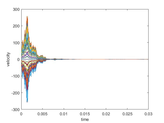
(a) Trajectories of the velocity $v^{1}$ for 100 particles.

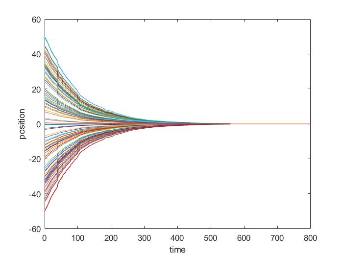
(b) Trajectories of the position $x^{1}$ for 100 particles.

Figure 2.1. The constant communication weight function.

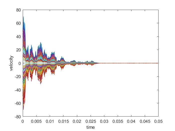
(a) Trajectories of the velocity $v^{1}$ for 100 particles.

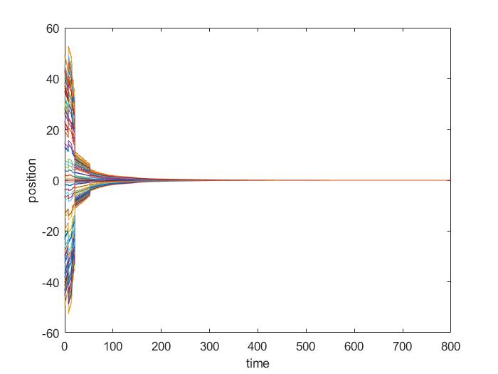
(b) Trajectories of the position $x^{1}$ for 100 particles.

Figure 2.2. The radially symmetric communication weight function.

From figure 2.1 and figure 2.2, we find that as time goes to infinity, all particles move at the same position and velocity. Then we confirm Theorem 2.1.

3. Kinetic C-S Vlasov-type equation

In this section, we consider the existence and asymptotic long-time behavior of solutions to the kinetic C-S Vlasov-type model in a harmonic field.

3.1. Existence of the global classical solution

Similar to [8, 15], the global existence of classical solution to kinetic C-S Vlasov-type model with noise can be established by introducing a new weighted Sobolev space. We state the main result without the proof. For a measurable function $f(x,v,t)$ in the phase space $\mathbb{R}^{2d}$, we set

$$\begin{aligned} &\|f\|_{L^{1}(x,v)}=\|(1+|x|^{2}+|v|^{2})f\|_{L^{1}(\mathbb{R}^{2d})},\\ &\|f\|_{L_{\alpha,x,v}^{2}}=\int_{\mathbb{R}^{2d}}(1+|x|^{2}+|v|^{2})^{\alpha}|f|^{2}dxdv,\quad\alpha\geq 0,\\ &\|f\|^{2}_{H_{\alpha}^{k}}:=\|f\|_{L_{\alpha,x,v}^{2}}+\sum\limits_{1\leq i+j\leq k}\|\partial_{x}^{i}\partial_{v}^{j}f\|_{L^{2}}^{2},\quad k\in\mathbb{N}\cup\{0\}.\end{aligned}$$

We define a function space where we will look for a classical solution: for $T>0$,

$$\mathcal{X}_{k,\alpha}(T):=\{f\in C(0,T;(H_{\alpha}^{k}\cap L^{1}_{(x,v)})(\mathbb{R}^{2d})):\sup\limits_{t\in[0,T)}(\|f(t)\|_{H_{\alpha}^{k}}+\|f(t)\|_{L^{1}_{(x,v)}})<\infty\}.$$

Theorem 3.1.

Let $T\in(0,\infty)$ be a positive constant and we assume that the initial configuration $f_{0}$ satisfies

$$f_{0}\in H_{\alpha}^{k}\cap L^{1}_{(x,v)},\ \ \mbox{for some positive constants}\ \ k>2+d,\ \ \alpha>\frac{d+2}{2}.$$

Then, there exists a unique global classical solution to the Cauchy problem of (1.3)-(1.4) in the function space $\mathcal{X}_{k,\alpha}(T)$.

3.2. Flocking and concentration behavior for the kinetic model

In this subsection, we derive a sufficient condition leading to a exponential flocking and concentration results for the kinetic model. Firstly, we present a lemma:

Lemma 3.1.

Let $f=f(x,v,t)$ be a smooth solution to (1.3)-(1.4) that quickly decays to zero at infinity. Then we have the following estimates:

1. The total mass is conserved:

   $$\begin{aligned} \frac{d}{dt}\int_{\mathbb{R}^{2d}}fdxdv=0,\quad t>0.\end{aligned}$$

2. We define the means $x_{c}=\int_{\mathbb{R}^{2d}}xfdxdv/\int_{\mathbb{R}^{2d}}fdxdv$ and $v_{c}=\int_{\mathbb{R}^{2d}}vfdxdv/\int_{\mathbb{R}^{2d}}fdxdv$. They are governed by the harmonic oscillators:

   $$\left\{\begin{split}&dx_{c}=v_{c}dt,\\ &dv_{c}=-x_{c}dt.\end{split}\right.$$ (3.1)

Proof.

Note that the equation in (1.3) can be rewritten in a divergent form:

$$\begin{split}&\partial_{t}f+\nabla_{x}\cdot(vf)+\nabla_{v}\cdot(L[f]f-xf-\sigma\nabla_{v}(|v-v_{c}|^{2}f))=0.\\ \end{split}$$ (3.2)

We integrate (3.2) in $(x,v)$ to obtain the conservation of mass.

W.o.l.g., we can assume that $\int_{\mathbb{R}^{2d}}fdxdv=1$ here. By the definition of $x_{c}$ and $v_{c}$, we have

$$\begin{split}&\frac{dx_{c}}{dt}=\int_{\mathbb{R}^{2d}}xf_{t}dxdv,\\ &\frac{dv_{c}}{dt}=\int_{\mathbb{R}^{2d}}vf_{t}dxdv.\end{split}$$

We multiply $x$ and $v$ with (3.2) respectively to get

$$\begin{split}&\partial_{t}(xf)+\nabla_{x}\cdot(x\otimes vf)-vf+\nabla_{v}\cdot\left[x\otimes\left(L[f]f-xf-\sigma\nabla_{v}(|v-v_{c}|^{2}f)\right)\right]=0\end{split}$$ (3.3)

and

$$\begin{split}&\partial_{t}(vf)+\!\nabla_{x}\!\cdot(v\otimes vf)+\nabla_{v}\cdot\left[v\otimes L[f]f\!-\sigma v\otimes\nabla_{v}(|v-v_{c}|^{2}f)-x\otimes vf\right]+xf\!\\ &\quad\quad\quad\quad\qquad\quad\quad\quad\quad=L[f]f-\sigma\nabla_{v}(|v-v_{c}|^{2}f).\end{split}$$ (3.4)

Then we integrate the relation in (LABEL:r1)-(LABEL:r2) and use

$$\begin{split}&\int_{\mathbb{R}^{2d}}L[f]fdvdx=-\kappa\int_{\mathbb{R}^{4d}}\psi(|x-y|)(v-v_{*})f(y,v_{*},t)f(x,v,t)dvdv_{*}dydx=0\end{split}$$

to obtain (3.1). ∎

To prove a flocking and concentration estimate for the kinetic model, we introduce a Lyapunov functional

$$\tilde{\mathcal{L}}[f](t):=\int_{\mathbb{R}^{2d}}\left(\frac{1}{2}|x-x_{c}|^{2}+\frac{1}{2}|v-v_{c}|^{2}+\epsilon(x-x_{c})\cdot(v-v_{c})\right)fdxdv,\quad|\epsilon|\leq\frac{1}{2}.$$ (3.5)

It is equivalent to the standard Lyapunov variance functional measuring the position and velocity variances of the kinetic density function $f$:

$$\mathcal{L}[f](t):=\int_{\mathbb{R}^{2d}}\left(|x-x_{c}|^{2}+|v-v_{c}|^{2}\right)fdxdv,$$ (3.6)

i.e., $\frac{3}{16}\mathcal{L}[f](t)\leq\tilde{\mathcal{L}}[f](t)\leq\frac{3}{4}\mathcal{L}[f](t).$

Theorem 3.2.

Suppose that the communication weight function $\psi$ satisfies the following positivity and boundedness conditions: there exist positive constants $\psi_{M}$ and $\psi_{m}$ such that

$$\begin{aligned} 0<\psi_{m}\leq\psi(s)\leq\psi_{M},\quad s\geq 0,\end{aligned}$$

and let $f=f(x,v,t)$ be a classical solution to (1.3) that quickly decays to zero at infinity and satisfies the finite second moments

$$\begin{aligned} \int_{\mathbb{R}^{2d}}(1+|v-v_{c}|^{2}+|x-x_{c}|^{2})f(x,v,t)dxdv<\infty,\quad t\geq 0.\end{aligned}$$

Then, the following estimates hold:

1. If $\kappa>\frac{d\sigma}{\psi_{m}||f_{0}||_{L^{1}}}$, there exists a positive constant $C_{m}:=\min\left\{\frac{1}{4},\frac{\kappa\psi_{m}||f_{0}||_{L^{1}}-d\sigma}{4(1+2(\kappa\psi_{M})^{2})}\right\}$, such that

   $$\begin{aligned} &\mathcal{L}[f](t)\leq 4\mathcal{L}[f_{0}]e^{-\frac{4}{3}C_{m}t}.\end{aligned}$$ (3.7)

2. If $\kappa<\frac{d\sigma}{\psi_{M}||f_{0}||_{L^{1}}}$, there exists a positive constant $C_{M}:=\min\left\{\frac{1+2(\kappa\psi_{M})^{2}}{2},\frac{d\sigma-\kappa\psi_{M}||f_{0}||_{L^{1}}}{2}\right\}$, such that

   $$\begin{aligned} &\mathcal{L}[f](t)\geq\frac{1}{4}\mathcal{L}[f_{0}]e^{\frac{4}{3}C_{M}t}.\end{aligned}$$ (3.8)

Proof.

We estimate each component in (3.5):
$\bullet$ (Estimate for $\int_{\mathbb{R}^{2d}}|x-x_{c}|^{2}fdxdv$):  By straightforward calculations, we get

$$\begin{aligned} \frac{d}{dt}\left(\int_{\mathbb{R}^{2d}}|x-x_{c}|^{2}fdxdv\right)&=-2\int_{\mathbb{R}^{2d}}(x-x_{c})\cdot\frac{dx_{c}}{dt}fdxdv+\int_{\mathbb{R}^{2d}}|x-x_{c}|^{2}f_{t}dxdv\\ &=\int_{\mathbb{R}^{2d}}|x-x_{c}|^{2}f_{t}dxdv,\\ \end{aligned}$$ (3.9)

where the first term in (3.9) vanished by the definition of $x_{c}$ in Lemma 3.1. Therefore (3.9) can be estimated as follows:

$$\begin{aligned} \frac{d}{dt}\left(\int_{\mathbb{R}^{2d}}|x-x_{c}|^{2}fdxdv\right)&=\int_{\mathbb{R}^{2d}}|x-x_{c}|^{2}f_{t}dxdv=2\int_{\mathbb{R}^{2d}}(x-x_{c})\cdot vfdxdv\\ &=2\int_{\mathbb{R}^{2d}}(x-x_{c})\cdot(v-v_{c})fdxdv,\end{aligned}$$ (3.10)

where we used $\int_{\mathbb{R}^{2d}}(x-x_{c})fdxdv=0$.
$\bullet$ (Estimate for $\int_{\mathbb{R}^{2d}}|v-v_{c}|^{2}fdxdv$): We calculate the derivative of it in a direct way to obtain

$$\begin{aligned} &\frac{d}{dt}\left(\int_{\mathbb{R}^{2d}}|v-v_{c}|^{2}fdxdv\right)=\int_{\mathbb{R}^{2d}}|v-v_{c}|^{2}f_{t}dxdv\\ &=2\!\!\int_{\mathbb{R}^{2d}}\!(v\!-\!v_{c})\cdot(L[f]f)dxdv\!+\!2d\sigma\!\!\int_{\mathbb{R}^{2d}}\!|v\!-\!v_{c}|^{2}fdxdv\!-\!2\int_{\mathbb{R}^{2d}}\!(x\!-\!x_{c})\!\cdot\!(v\!-\!v_{c})fdxdv,\end{aligned}$$ (3.11)

where we used $\int_{\mathbb{R}^{2d}}(v-v_{c})fdxdv=0$. Note that the first term on the R. H. S. of (LABEL:1.2) can be estimated as follows:

$$\begin{aligned} &\int_{\mathbb{R}^{2d}}(v-v_{c})\cdot(L[f]f)dxdv\\ &=-\kappa\int_{\mathbb{R}^{4d}}\psi(|x-y|)(v-v_{c})\cdot(v-v_{\ast})f(y,v_{\ast},t)f(x,v,t)dv_{\ast}dvdydx\\ &=\kappa\int_{\mathbb{R}^{4d}}\psi(|x-y|)(v_{\ast}-v_{c})\cdot(v-v_{\ast})f(y,v_{\ast},t)f(x,v,t)dv_{\ast}dvdydx\\ &=-\frac{\kappa}{2}\int_{\mathbb{R}^{4d}}\psi(|x-y|)|v-v_{\ast}|^{2}f(y,v_{\ast},t)f(x,v,t)dv_{\ast}dvdydx.\\ \end{aligned}$$ (3.12)

Then, we combine (LABEL:1.2) and (LABEL:1.3) to obtain:

$$\begin{aligned} &\frac{d}{dt}\left(\int_{\mathbb{R}^{2d}}|v-v_{c}|^{2}fdxdv\right)\\ &=-\kappa\int_{\mathbb{R}^{4d}}\psi(|x-y|)|v-v_{\ast}|^{2}f(y,v_{\ast},t)f(x,v,t)dv_{\ast}dvdydx\\ &\quad+2d\sigma\int_{\mathbb{R}^{2d}}|v-v_{c}|^{2}fdxdv-2\int_{\mathbb{R}^{2d}}(x-x_{c})\cdot(v-v_{c})fdxdv.\end{aligned}$$ (3.13)

$\bullet$ (Estimate for $\int_{\mathbb{R}^{2d}}(x-x_{c})\cdot(v-v_{c})fdxdv$): We calculate the cross term directly:

$$\begin{aligned} &\frac{d}{dt}\left(\int_{\mathbb{R}^{2d}}(x-x_{c})\cdot(v-v_{c})fdxdv\right)=\int_{\mathbb{R}^{2d}}(x-x_{c})\cdot(v-v_{c})f_{t}dxdv\\ &=\int_{\mathbb{R}^{2d}}|v-v_{c}|^{2}fdxdv-\int_{\mathbb{R}^{2d}}|x-x_{c}|^{2}fdxdv+\int_{\mathbb{R}^{2d}}(x-x_{c})\cdot L[f]fdxdv,\end{aligned}$$ (3.14)

where we used $\int_{\mathbb{R}^{2d}}(x-x_{c})fdxdv=0$ and $\int_{\mathbb{R}^{2d}}(v-v_{c})fdxdv=0$. The third term on the R.H.S. of (LABEL:1.6) can be estimated as follows:

$$\begin{aligned} &\int_{\mathbb{R}^{2d}}(x-x_{c})\cdot(L[f]f)dxdv\\ &=-\kappa\int_{\mathbb{R}^{4d}}\psi(|x-y|)(x-x_{c})\cdot(v-v_{\ast})f(y,v_{\ast},t)f(x,v,t)dv_{\ast}dvdydx\\ &=-\kappa\int_{\mathbb{R}^{4d}}\psi(|x-y|)(x-x_{c})\cdot(v-v_{c})f(y,v_{\ast},t)f(x,v,t)dv_{\ast}dvdydx\\ &\quad-\kappa\int_{\mathbb{R}^{4d}}\psi(|x-y|)(x-x_{c})\cdot(v_{c}-v_{\ast})f(y,v_{\ast},t)f(x,v,t)dv_{\ast}dvdydx\\ &\leq\kappa\psi_{M}\int_{\mathbb{R}^{4d}}\left(\frac{|x-x_{c}|^{2}}{4\kappa\psi_{M}}+\kappa\psi_{M}|v-v_{c}|^{2}\right)f(y,v_{\ast},t)f(x,v,t)dv_{\ast}dvdydx\\ &\quad+\kappa\psi_{M}\int_{\mathbb{R}^{4d}}\left(\frac{|x-x_{c}|^{2}}{4\kappa\psi_{M}}+\kappa\psi_{M}|v_{c}-v_{\ast}|^{2}\right)f(y,v_{\ast},t)f(x,v,t)dv_{\ast}dvdydx\\ &=\frac{1}{2}\int_{\mathbb{R}^{2d}}|x-x_{c}|^{2}f(x,v,t)dxdv+2(\kappa\psi_{M})^{2}\int_{\mathbb{R}^{2d}}|v-v_{c}|^{2}f(x,v,t)dxdv,\end{aligned}$$ (3.15)

where we used $(x-x_{c})\cdot(v-v_{c})\leq\frac{|x-x_{c}|^{2}}{4\kappa\psi_{M}}+\kappa\psi_{M}|v-v_{c}|^{2}$ and $(x-x_{c})\cdot(v_{c}-v_{\ast})\leq\frac{|x-x_{c}|^{2}}{4\kappa\psi_{M}}+\kappa\psi_{M}|v_{c}-v_{\ast}|^{2}$. Then, we combine (LABEL:1.6) and (LABEL:1.7) to obtain an estimate for the cross term:

$$\begin{aligned} &\frac{d}{dt}\left(\int_{\mathbb{R}^{2d}}(x-x_{c})\cdot(v-v_{c})fdxdv\right)\\ &\leq(1+2(\kappa\psi_{M})^{2})\int_{\mathbb{R}^{2d}}|v-v_{c}|^{2}fdxdv-\frac{1}{2}\int_{\mathbb{R}^{2d}}|x-x_{c}|^{2}fdxdv.\end{aligned}$$ (3.16)

Finally, we take $\frac{1}{2}\eqref{l}+\frac{1}{2}\eqref{1.4}+\epsilon\eqref{1.8}$ to obtain a differential inequality for $\tilde{\mathcal{L}}[f](t)$:

$$\begin{aligned} &\frac{d\tilde{\mathcal{L}}[f](t)}{dt}=\frac{d}{dt}\int_{\mathbb{R}^{2d}}\left(\frac{1}{2}|x-x_{c}|^{2}+\frac{1}{2}|v-v_{c}|^{2}+\epsilon(x-x_{c})\cdot(v-v_{c})\right)fdxdv\\ &\leq\!-(\kappa\psi_{m}||f_{0}||_{L^{1}}\!-\!d\sigma\!-\!(1+2(\kappa\psi_{M})^{2})\epsilon)\!\int_{\mathbb{R}^{2d}}|v\!-\!v_{c}|^{2}fdxdv\!-\!\frac{\epsilon}{2}\!\int_{\mathbb{R}^{2d}}|x\!-\!x_{c}|^{2}fdxdv,\end{aligned}$$ (3.17)

where we used $\int_{\mathbb{R}^{2d}}(v-v_{c})fdxdv=0$ and $|v-v_{\ast}|^{2}=|v-v_{c}+v_{c}-v_{\ast}|^{2}$. One can simplify (LABEL:1.9) by taking $\epsilon=\min\{\frac{1}{2},\frac{\kappa\psi_{m}||f_{0}||_{L^{1}}-d\sigma}{2(1+2(\kappa\psi_{M})^{2})}\}$:

$$\begin{aligned} &\frac{d}{dt}\int_{\mathbb{R}^{2d}}\left(\frac{1}{2}|x-x_{c}|^{2}+\frac{1}{2}|v-v_{c}|^{2}+\epsilon(x-x_{c})\cdot(v-v_{c})\right)fdxdv\\ &\leq-C_{m}\int_{\mathbb{R}^{2d}}(|x-x_{c}|^{2}+|v-v_{c}|^{2})fdxdv,\end{aligned}$$ (3.18)

where $C_{m}=\min\{\frac{\epsilon}{2},\frac{\kappa\psi_{m}||f_{0}||_{L^{1}}-d\sigma}{2}\}$. In (LABEL:1.10), we apply the Grönwall’s inequality to get

$$\begin{aligned} &\tilde{\mathcal{L}}[f](t)\leq\tilde{\mathcal{L}}[f_{0}]e^{-\frac{4}{3}C_{m}t}\end{aligned}$$

and conclude the first result (3.7).

On the other hand, we derive

$$\begin{aligned} &\int_{\mathbb{R}^{2d}}(x-x_{c})\cdot(L[f]f)dxdv\\ &=-\kappa\int_{\mathbb{R}^{4d}}\psi(|x-y|)(x-x_{c})\cdot(v-v_{c})f(y,v_{\ast},t)f(x,v,t)dv_{\ast}dvdydx\\ &\quad-\kappa\int_{\mathbb{R}^{4d}}\psi(|x-y|)(x-x_{c})\cdot(v_{c}-v_{\ast})f(y,v_{\ast},t)f(x,v,t)dv_{\ast}dvdydx\\ &\geq-\kappa\psi_{M}\int_{\mathbb{R}^{4d}}\left[\kappa\psi_{M}|x-x_{c}|^{2}+\frac{|v-v_{c}|^{2}}{4\kappa\psi_{M}}\right]f(y,v_{\ast},t)f(x,v,t)dv_{\ast}dvdydx\\ &\quad-\kappa\psi_{M}\int_{\mathbb{R}^{4d}}\left[\kappa\psi_{M}|x-x_{c}|^{2}+\frac{|v_{c}-v_{\ast}|^{2}}{4\kappa\psi_{M}}\right]f(y,v_{\ast},t)f(x,v,t)dv_{\ast}dvdydx\\ &=-2(\kappa\psi_{M})^{2}\int_{\mathbb{R}^{2d}}|x-x_{c}|^{2}f(x,v,t)dxdv-\frac{1}{2}\int_{\mathbb{R}^{2d}}|v-v_{c}|^{2}f(x,v,t)dxdv.\end{aligned}$$ (3.19)

Then, we combine (LABEL:1.6) and (LABEL:2.1) to get an estimate for the cross term:

$$\begin{aligned} &\frac{d}{dt}\left(\int_{\mathbb{R}^{2d}}(x-x_{c})\cdot(v-v_{c})fdxdv\right)\\ &\geq\frac{1}{2}\int_{\mathbb{R}^{2d}}|v-v_{c}|^{2}fdxdv-(1+2(\kappa\psi_{M})^{2})\int_{\mathbb{R}^{2d}}|x-x_{c}|^{2}fdxdv.\end{aligned}$$ (3.20)

Finally, we take $\frac{1}{2}\eqref{l}+\frac{1}{2}\eqref{1.4}+\epsilon\eqref{2.2}$ to obtain a differential inequality $\tilde{\mathcal{L}}[f](t)$:

$$\begin{aligned} &\frac{d\tilde{\mathcal{L}}[f](t)}{dt}=\frac{d}{dt}\int_{\mathbb{R}^{2d}}\left(\frac{1}{2}|x-x_{c}|^{2}+\frac{1}{2}|v-v_{c}|^{2}+\epsilon(x-x_{c})\cdot(v-v_{c})\right)fdxdv\\ &\geq-\left(\kappa\psi_{M}||f_{0}||_{L^{1}}-d\sigma-\frac{1}{2}\epsilon\right)\!\!\int_{\mathbb{R}^{2d}}|v-v_{c}|^{2}fdxdv-(1+2(\kappa\psi_{M})^{2})\epsilon\int_{\mathbb{R}^{2d}}|x-x_{c}|^{2}fdxdv.\end{aligned}$$ (3.21)

One can simplify (LABEL:2.3) by taking $\epsilon=\max\{-\frac{1}{2},\kappa\psi_{M}||f_{0}||_{L^{1}}-d\sigma\}$:

$$\begin{aligned} &\frac{d}{dt}\int_{\mathbb{R}^{2d}}\left(\frac{1}{2}|x-x_{c}|^{2}+\frac{1}{2}|v-v_{c}|^{2}+\epsilon(x-x_{c})\cdot(v-v_{c})\right)fdxdv\\ &\geq C_{M}\int_{\mathbb{R}^{2d}}(|x-x_{c}|^{2}+|v-v_{c}|^{2})fdxdv,\end{aligned}$$ (3.22)

where $C_{M}=\min\{-(1+2(\kappa\psi_{M})^{2})\epsilon,\frac{d\sigma-\kappa\psi_{M}||f_{0}||_{L^{1}}}{2}\}>0$. In (LABEL:2.4), we apply the Grönwall’s inequality to get

$$\begin{aligned} &\tilde{\mathcal{L}}[f](t)\geq\tilde{\mathcal{L}}[f_{0}]e^{\frac{4}{3}C_{M}t}\end{aligned}$$

and conclude the second result (3.8). ∎

4. Mean-field limit: from stochastic particle system to the kinetic C-S Vlasov-type equation

In this section, we present a uniform-in-time mean-field limit from the stochastic C-S model to the kinetic C-S Vlasov-type equation in a large population limit $N\to\infty$ in the whole time-interval $[0,\infty)$, using the so called C-S McKean process. Note that the Galilean invariance is hold because of harmonic oscillators (2.1) or (3.1). Similar to [14], it is sufficient to study with $(x_{c}(0),v_{c}(0))=(0,0)$, which implies $(x_{c}(t),v_{c}(t))=(0,0)$. Recall that the stochastic particle model is

$$\left\{\begin{aligned} &dx_{t}^{i}=v_{t}^{i}dt,\qquad t>0,\quad 1\leq i\leq N,\\ &dv_{t}^{i}=-\frac{\kappa}{N}\sum\limits_{j=1}^{N}\psi(|x_{t}^{j}-x_{t}^{i}|)(v_{t}^{i}-v_{t}^{j})dt-x_{t}^{i}dt+\sqrt{2\sigma}v_{t}^{i}dW_{t},\\ &\sum\limits_{i=1}^{N}x_{t}^{i}=0,\quad\sum\limits_{i=1}^{N}v_{t}^{i}=0.\end{aligned}\right.$$ (4.1)

By symmetry of the initial configurations and the pairwise interaction of particles, all particles have the same distribution on $\mathbb{R}^{2d}$ at time $t$, which will be denoted $f^{1,N}$.

To study the behavior of the stochastic C-S model (LABEL:SCS) for a large population $N\gg 1$, we use the concept of “propagation of chaos” originating from Kac’s Markovian model of gas dynamics. The propagation of chaos refers to the phenomenon that for any finite number of particles, each particles follow the “McKean process” $(\bar{x}_{t}^{i},\bar{v}_{t}^{i},f)$, which is given by the solution of the following symmetric particle system

$$\left\{\begin{aligned} &d\bar{x}_{t}^{i}=\bar{v}_{t}^{i}dt,\qquad t>0,\quad 1\leq i\leq N,\\ &d\bar{v}_{t}^{i}=-\kappa\psi*f(\bar{x}_{t}^{i},\bar{v}_{t}^{i})dt-\bar{x}_{t}^{i}dt+\sqrt{2\sigma}\bar{v}_{t}^{i}dW_{t},\\ &f=law(\bar{x}_{t}^{i},\bar{v}_{t}^{i}),\quad(\bar{x}_{t}^{i}(0),\bar{v}_{t}^{i}(0))=(x_{0}^{i},v_{0}^{i}),\end{aligned}\right.$$ (4.2)

where $\psi*f(x,v):=\int_{\mathbb{R}^{2d}}\psi(|x-y|)(v-v_{\ast})f(y,v_{\ast})dydv_{\ast}$ is the convolution between $\psi$ and $f$ in the phase space. By the way, when the McKean process acts on the empirical measure $\mu^{N}_{t}=\frac{1}{N}\sum\limits_{i=1}^{N}\delta_{(x_{t}^{i},v_{t}^{i})}$, the system (LABEL:MK1) can be reduced to the stochastic system (LABEL:SCS).

The system (LABEL:MK1) consists of $N$ equations which can be solved independently of each other. Each of them involves the condition that $f$ is the distribution of $(\bar{x}_{t}^{i},\bar{v}_{t}^{i})$, thus making it nonlinear. The system (LABEL:MK1) and the system (LABEL:SCS) have the same initial configurations and share the same Brownian motions. Note that the system (LABEL:MK1) is not anymore an SDE system, and the dynamics between particles is now coupled through the law $f$. The law is the same for each particle. It is straightforward to check that $f$ is just the (weak) solution to the mean-field PDE model (1.3) by Itô’s formula. According to [2, 15], in order to verify the weak convergence from the empirical measure $\mu^{N}_{t}$ to $f$, i.e. the mean-field limit, it is sufficient to show that for any $t$, $\lim\limits_{N\to\infty}(E[|x_{t}^{i}-\bar{x}_{t}^{i}|^{2}]+E[|v_{t}^{i}-\bar{v}_{t}^{i}|^{2}])=0$, under the assumption of the well-posedness of both SDE and PDE systems.

Remark 4.1.

The estimate $\lim\limits_{N\to\infty}(E[|x_{t}^{i}-\bar{x}_{t}^{i}|^{2}]+E[|v_{t}^{i}-\bar{v}_{t}^{i}|^{2}])=0$ classically ensures quantitative estimates on ( see [2, 15] for details)

1. The convergence in $N$ of the law $f^{1,N}$ at time $t$ of any (by symmetry) of the processes $(x_{t}^{i},v_{t}^{i})$ towards $f$;

2. The propagation of chaos: for all fixed $k$, the law $f^{k,N}$ for any $k$ particles $(x_{t}^{i},v_{t}^{i})$ converges to the tensor product $f^{\otimes k}$ as $N$ tends to infinity;

3. The convergence of the empirical measure $\mu^{N}_{t}$ at time $t$ of the particle system (LABEL:SCS) towards $f$.

4.1. Exponential decay in time estimate for the limit process

In this subsection, we derive a uniform-in-time boundedness and decay property for the difference between two processes (LABEL:SCS) and (LABEL:MK1) driven by the same Brownian motion and initial configuration.

Firstly, we need to derive the flocking and concentration result in the probabilistic sense for the McKean process $(\bar{x}_{t}^{i},\bar{v}_{t}^{i})$ for preparation. We set

$$\begin{aligned} &a(x,t):=\int_{\mathbb{R}^{2d}}\psi(|x-y|)f(y,v_{\ast},t)dv_{\ast}dy,\\ &b(x,t):=\int_{\mathbb{R}^{2d}}v_{\ast}\psi(|x-y|)f(y,v_{\ast},t)dv_{\ast}dy.\end{aligned}$$

Then we have

$$\begin{aligned} &\psi_{m}||f_{0}||_{L^{1}}\leq a(x,t)\leq\psi_{M}||f_{0}||_{L^{1}},\\ &|b(x,t)|\leq 2\psi_{M}e^{-\frac{2C_{m}t}{3}}\sqrt{||f_{0}||_{L^{1}}||(|v|^{2}+|x|^{2})f_{0}||_{L^{1}}},\\ \end{aligned}$$ (4.3)

and (LABEL:MK1) becomes

$$\left\{\begin{aligned} &d\bar{x}_{t}^{i}=\bar{v}_{t}^{i}dt,\qquad t>0,\quad 1\leq i\leq N,\\ &d\bar{v}_{t}^{i}=-\kappa(a(\bar{x}_{t}^{i},t)\bar{v}_{t}^{i}-b(\bar{x}_{t}^{i},t))dt-\bar{x}_{t}^{i}dt+\sqrt{2\sigma}\bar{v}_{t}^{i}dW_{t},\\ &f=law(\bar{x}_{t}^{i},\bar{v}_{t}^{i}),\quad(\bar{x}_{t}^{i}(0),\bar{v}_{t}^{i}(0))=(x_{0}^{i},v_{0}^{i}).\end{aligned}\right.$$ (4.4)

Now we derive a differential inequality.

Lemma 4.1.

Suppose that the communication weight function $\psi$, $\kappa$, $\sigma$ and initial configuration $f_{0}$ satisfy the conditions: there exist positive constants $\psi_{m},\psi_{M}$ such that

$$\begin{aligned} &0<\psi_{m}\leq\psi\leq\psi_{M},\quad\kappa\psi_{m}||f_{0}||_{L^{1}}>d\sigma,\quad\int_{\mathbb{R}^{2d}}(1+|v|^{2}+|x|^{2})f_{0}dxdv<\infty.\end{aligned}$$

Then, we have

$$\begin{aligned} \frac{d}{dt}E\left[\frac{1}{2}|\bar{x}_{t}^{i}|^{2}+\frac{1}{2}|\bar{v}_{t}^{i}|^{2}+\epsilon\bar{x}_{t}^{i}\cdot\bar{v}_{t}^{i}\right]\leq-\eta E\left[|\bar{x}_{t}^{i}|^{2}+|\bar{v}_{t}^{i}|^{2}\right]+\lambda e^{-\frac{4}{3}C_{m}t},\end{aligned}$$

where $\epsilon=\min\{\frac{1}{2},\frac{\kappa\psi_{m}||f_{0}||_{L^{1}}-\sigma}{2(1+2(\kappa\psi_{M})^{2})}\}$, $\eta=\min\{\frac{1}{2}\epsilon,\frac{1}{4}(\kappa\psi_{m}||f_{0}||_{L^{1}}-\sigma)\}$, $\delta=\frac{\kappa\psi_{m}||f_{0}||_{L^{1}}-\sigma}{\kappa}$, $\lambda=(\frac{2}{\delta}+4\epsilon\kappa)\kappa\psi_{M}^{2}||f_{0}||_{L^{1}}||(|v|^{2}+|x|^{2})f_{0}||_{L^{1}}$ and $C_{m}$ is given in Theorem 3.2.

Proof.

$\bullet$ (Estimate for $d|\bar{x}_{t}^{i}|^{2}$):  By Itô’s formula, we can obtain

$$\begin{aligned} &d|\bar{x}_{t}^{i}|^{2}=2\bar{x}_{t}^{i}\cdot d\bar{x}_{t}^{i}+d\bar{x}_{t}^{i}\cdot d\bar{x}_{t}^{i}=2\bar{x}_{t}^{i}\cdot\bar{v}_{t}^{i}dt.\end{aligned}$$ (4.5)

$\bullet$ (Estimate for $d|\bar{v}_{t}^{i}|^{2}$): By direct calculation, we have

$$\begin{aligned} d|\bar{v}_{t}^{i}|^{2}=2\bar{v}_{t}^{i}\cdot d\bar{v}_{t}^{i}+d\bar{v}_{t}^{i}\cdot d\bar{v}_{t}^{i}:=\mathcal{I}_{11}+\mathcal{I}_{12}.\\ \end{aligned}$$

We use (LABEL:MK2)₂ and (LABEL:E) to obtain

$$\begin{aligned} \mathcal{I}_{11}&=2\bar{v}_{t}^{i}\cdot d\bar{v}_{t}^{i}\\ &=-2\kappa(a(\bar{x}_{t}^{i},t)|\bar{v}_{t}^{i}|^{2}-b(\bar{x}_{t}^{i},t)\bar{v}_{t}^{i})dt-2\bar{x}_{t}^{i}\cdot\bar{v}_{t}^{i}dt+2\sqrt{2\sigma}|\bar{v}_{t}^{i}|^{2}dW_{t}\\ &\leq-2\kappa\left(\psi_{m}||f_{0}||_{L^{1}}-\frac{\delta}{2}\right)|\bar{v}_{t}^{i}|^{2}dt+\frac{4\kappa\psi_{M}^{2}}{\delta}e^{-\frac{4}{3}C_{m}t}||f_{0}||_{L^{1}}||(|v|^{2}+|x|^{2})f_{0}||_{L^{1}}dt\\ &\quad-2\bar{x}_{t}^{i}\cdot\bar{v}_{t}^{i}dt+2\sqrt{2\sigma}|\bar{v}_{t}^{i}|^{2}dW_{t},\end{aligned}$$ (4.6)

where we used the $\delta$-Young inequailty and $\delta$ will be defined later:

$$\begin{aligned} |\bar{v}_{t}^{i}||b(\bar{x}_{t}^{i},t)|\leq\frac{\delta}{2}|\bar{v}_{t}^{i}|^{2}+\frac{2}{\delta}\psi_{M}^{2}e^{-\frac{4}{3}C_{m}t}||f_{0}||_{L^{1}}||(|v|^{2}+|x|^{2})f_{0}||_{L^{1}}.\end{aligned}$$

The term $\mathcal{I}_{12}$ can be easily obtained as follows:

$$\begin{aligned} \mathcal{I}_{12}&=d\bar{v}_{t}^{i}\cdot d\bar{v}_{t}^{i}=2\sigma|\bar{v}_{t}^{i}|^{2}dt.\end{aligned}$$ (4.7)

We combine (4.6) and (4.7) to have

$$\begin{aligned} d|\bar{v}_{t}^{i}|^{2}&\leq\!-2\kappa\!\left(\psi_{m}||f_{0}||_{L^{1}}\!-\!\frac{\delta}{2}\!-\!\frac{\sigma}{\kappa}\!\right)|\bar{v}_{t}^{i}|^{2}dt\!+\frac{4\kappa\psi_{M}^{2}}{\delta}e^{-\frac{4}{3}C_{m}t}||f_{0}||_{L^{1}}||(|v|^{2}+|x|^{2})f_{0}||_{L^{1}}dt\\ &\quad-2\bar{x}_{t}^{i}\cdot\bar{v}_{t}^{i}dt+2\sqrt{2\sigma}|\bar{v}_{t}^{i}|^{2}dW_{t}.\end{aligned}$$ (4.8)

$\bullet$ (Estimate for $d(\bar{x}_{t}^{i}\cdot\bar{v}_{t}^{i})$): Now we estimate the cross term:

$$\begin{aligned} d(\bar{x}_{t}^{i}\cdot\bar{v}_{t}^{i})&=\bar{x}_{t}^{i}\cdot d\bar{v}_{t}^{i}+\bar{v}_{t}^{i}\cdot d\bar{x}_{t}^{i}+d\bar{x}_{t}^{i}\cdot d\bar{v}_{t}^{i}\\ &=\bar{x}_{t}^{i}\cdot[-\kappa(a(\bar{x}_{t}^{i},t)\bar{v}_{t}^{i}-b(\bar{x}_{t}^{i},t))dt-\bar{x}_{t}^{i}dt+\sqrt{2\sigma}\bar{v}_{t}^{i}dW_{t}]+|\bar{v}_{t}^{i}|^{2}dt\\ &=-\kappa\bar{x}_{t}^{i}\cdot(a(\bar{x}_{t}^{i},t)\bar{v}_{t}^{i}-b(\bar{x}_{t}^{i},t))dt+\sqrt{2\sigma}\bar{x}_{t}^{i}\cdot\bar{v}_{t}^{i}dW_{t}-|\bar{x}_{t}^{i}|^{2}dt+|\bar{v}_{t}^{i}|^{2}dt\\ &:=\mathcal{I}_{21}dt+\sqrt{2\sigma}\bar{x}_{t}^{i}\cdot\bar{v}_{t}^{i}dW_{t}-|\bar{x}_{t}^{i}|^{2}dt+|\bar{v}_{t}^{i}|^{2}dt.\end{aligned}$$ (4.9)

$\mathcal{I}_{21}$ can be estimated as follows:

$$\begin{aligned} &|\mathcal{I}_{21}|=\kappa|\bar{x}_{t}^{i}\cdot(a(\bar{x}_{t}^{i},t)\bar{v}_{t}^{i}-b(\bar{x}_{t}^{i},t))|\\ &\leq\kappa\psi_{M}||f_{0}||_{L^{1}}\left(\kappa\psi_{M}||f_{0}||_{L^{1}}|v_{t}^{i}|^{2}+\frac{1}{4\kappa\psi_{M}||f_{0}||_{L^{1}}}|x_{t}^{i}|^{2}\right)+\kappa|\bar{x}_{t}^{i}||b(\bar{x}_{t}^{i},t)|\\ &\leq\left[\frac{1}{4}|\bar{x}_{t}^{i}|^{2}+(\kappa\psi_{M}||f_{0}||_{L^{1}})^{2}|\bar{v}_{t}^{i}|^{2}\right]\!+\!2\kappa|\bar{x}_{t}^{i}|\psi_{M}e^{-\frac{2C_{m}t}{3}}\!\sqrt{||f_{0}||_{L^{1}}||(|v|^{2}+|x|^{2})f_{0}||_{L^{1}}}\\ &\leq\left[\frac{1}{2}|\bar{x}_{t}^{i}|^{2}+(\kappa\psi_{M}||f_{0}||_{L^{1}})^{2}|\bar{v}_{t}^{i}|^{2}\right]+4\kappa^{2}\psi_{M}^{2}e^{-\frac{4}{3}C_{m}t}||f_{0}||_{L^{1}}||(|v|^{2}+|x|^{2})f_{0}||_{L^{1}}.\end{aligned}$$ (4.10)

By inserting (LABEL:51) into (4.9), we have

$$\begin{aligned} d(\bar{x}_{t}^{i}\cdot\bar{v}_{t}^{i})&\leq-\frac{1}{2}|\bar{x}_{t}^{i}|^{2}dt+\left[(\kappa\psi_{M}||f_{0}||_{L^{1}})^{2}+1\right]|\bar{v}_{t}^{i}|^{2}dt\\ &\quad+4\kappa^{2}\psi_{M}^{2}e^{-\frac{4}{3}C_{m}t}||f_{0}||_{L^{1}}||(|v|^{2}+|x|^{2})f_{0}||_{L^{1}}dt+\sqrt{2\sigma}\bar{x}_{t}^{i}\cdot\bar{v}_{t}^{i}dW_{t}.\end{aligned}$$ (4.11)

Now we take a combination $\frac{1}{2}\eqref{q1}+\frac{1}{2}\eqref{q2}+\epsilon\eqref{q3}$ to get the following differential inequality:

$$\begin{aligned} &dE\left(\frac{1}{2}|\bar{x}_{t}^{i}|^{2}+\frac{1}{2}|\bar{v}_{t}^{i}|^{2}+\epsilon\bar{x}_{t}^{i}\cdot\bar{v}_{t}^{i}\right)\\ &\leq-\left[\kappa\psi_{m}||f_{0}||_{L^{1}}-\sigma-\frac{\delta\kappa}{2}-((\kappa\psi_{M}||f_{0}||_{L^{1}})^{2}+1)\epsilon\right]E[|\bar{v}_{t}^{i}|^{2}]dt-\frac{\epsilon}{2}E[|\bar{x}_{t}^{i}|^{2}]dt\\ &\quad+\left(\frac{2}{\delta}+4\epsilon\kappa\right)\kappa\psi_{M}^{2}e^{-\frac{4}{3}C_{m}t}||f_{0}||_{L^{1}}||(|v|^{2}+|x|^{2})f_{0}||_{L^{1}}dt.\end{aligned}$$

We take $\delta:=\frac{\kappa\psi_{m}||f_{0}||_{L^{1}}-\sigma}{\kappa}$, $\epsilon:=\min\{\frac{1}{2},\frac{1}{4}\frac{\kappa\psi_{m}||f_{0}||_{L^{1}}-\sigma}{(\kappa\psi_{M}||f_{0}||_{L^{1}})^{2}+1}\}$ and obtain

$$\begin{aligned} dE\left[\frac{1}{2}|\bar{x}_{t}^{i}|^{2}+\frac{1}{2}|\bar{v}_{t}^{i}|^{2}+\epsilon\bar{x}_{t}^{i}\cdot\bar{v}_{t}^{i}\right]\leq-\eta E\left[|\bar{x}_{t}^{i}|^{2}+|\bar{v}_{t}^{i}|^{2}\right]dt+\lambda e^{-\frac{4}{3}C_{m}t}dt,\\ \end{aligned}$$ (4.12)

where $\eta:=\min\{\frac{1}{2}\epsilon,\frac{1}{4}(\kappa\psi_{m}||f_{0}||_{L^{1}}-\sigma)\},\lambda:=(\frac{2}{\delta}+4\epsilon\kappa)\kappa\psi_{M}^{2}||f_{0}||_{L^{1}}||(|v|^{2}+|x|^{2})f_{0}||_{L^{1}}$. ∎

Lemma 4.2.

Suppose that the communication weight function $\psi$, $\kappa$, $\sigma$ and initial configuration $f_{0}$ satisfy the conditions: there exist positive constants $\psi_{m},\psi_{M}$ such that

$$\begin{aligned} &0<\psi_{m}\leq\psi\leq\psi_{M},\quad\kappa\psi_{m}||f_{0}||_{L^{1}}>d\sigma,\quad\int_{\mathbb{R}^{2d}}(1+|v|^{2}+|x|^{2})f_{0}dxdv<\infty,\quad t\geq 0.\end{aligned}$$

Then we have

$$\begin{aligned} &E[|\bar{x}_{t}^{i}|^{2}+|\bar{v}_{t}^{i}|^{2}]\leq Ce^{-\frac{4}{3}C_{\ast}t},\end{aligned}$$

where $C_{\ast}=\min\{C_{m},\eta\}$ and $C$ is a constant which depends on initial configuration, $\psi$, $\kappa$ and $\sigma$.

Proof.

We set

$$\begin{aligned} &\mathcal{Z}_{t}:=|\bar{x}_{t}^{i}|^{2}+|\bar{v}_{t}^{i}|^{2}.\end{aligned}$$

Since $|\epsilon|\leq\frac{1}{2}$, the quantity $\frac{1}{2}|\bar{x}_{t}^{i}|^{2}+\frac{1}{2}|\bar{v}_{t}^{i}|^{2}+\epsilon\bar{x}_{t}^{i}\cdot\bar{v}_{t}^{i}$ is equivalent to $|\bar{x}_{t}^{i}|^{2}+|\bar{v}_{t}^{i}|^{2}$ :

$$\frac{3}{16}\mathcal{Z}_{t}\leq\frac{1}{2}|\bar{x}_{t}^{i}|^{2}+\frac{1}{2}|\bar{v}_{t}^{i}|^{2}+\epsilon\bar{x}_{t}^{i}\cdot\bar{v}_{t}^{i}\leq\frac{3}{4}\mathcal{Z}_{t}.$$

Then, it follows from (4.12) that $\frac{1}{2}|\bar{x}_{t}^{i}|^{2}+\frac{1}{2}|\bar{v}_{t}^{i}|^{2}+\epsilon\bar{x}_{t}^{i}\cdot\bar{v}_{t}^{i}$ satisfies the following SDE:

$$\begin{aligned} dE\left[\frac{1}{2}|\bar{x}_{t}^{i}|^{2}+\frac{1}{2}|\bar{v}_{t}^{i}|^{2}+\epsilon\bar{x}_{t}^{i}\cdot\bar{v}_{t}^{i}\right]\leq-\frac{4}{3}\eta E\left[\frac{1}{2}|\bar{x}_{t}^{i}|^{2}+\frac{1}{2}|\bar{v}_{t}^{i}|^{2}+\epsilon\bar{x}_{t}^{i}\cdot\bar{v}_{t}^{i}\right]dt+\lambda e^{-\frac{4}{3}C_{m}t}dt.\end{aligned}$$

Therefore, we obtain

$$\begin{aligned} &E[\mathcal{Z}_{t}]\leq 4E[\mathcal{Z}_{0}]e^{-\frac{4}{3}\eta t}+\frac{4\lambda}{\eta-C_{m}}(e^{-\frac{4}{3}C_{m}t}-e^{-\frac{4}{3}\eta t})\leq Ce^{-\frac{4}{3}C_{\ast}t},\end{aligned}$$

where $C_{\ast}=\min\{C_{m},\eta\}$ and $C$ is a general constant. Then we get the desired result. ∎

Now we are ready to state our result on the exponential decay in time estimate for the limit process.

Theorem 4.1.

Suppose that the communication weight function $\psi$, $\kappa$, $\sigma$ and initial configuration $f_{0}$ satisfy the conditions: there exist positive constants $\psi_{m},\psi_{M}$ such that

$$\begin{aligned} &0<\psi_{m}\leq\psi\leq\psi_{M},\quad\kappa\psi_{m}\min\{||f_{0}||_{L^{1}},1\}>d\sigma,\quad\int_{\mathbb{R}^{2d}}(1+|v|^{2}+|x|^{2})f_{0}dxdv<\infty\end{aligned}$$

and let $(x_{t}^{i},v_{t}^{i})$ and $(\bar{x}_{t}^{i},\bar{v}_{t}^{i},f)$ be solution processes to the systems in (LABEL:SCS) and (LABEL:MK2), respectively. Then, we have

$$\begin{aligned} &E[|x_{t}^{i}-\bar{x}_{t}^{i}|^{2}]+E[|v_{t}^{i}-\bar{v}_{t}^{i}|^{2}]\leq Ce^{-C_{3}t},\end{aligned}$$

where $C$ and $C_{3}$ depend on initial configuration, $\psi$, $\kappa$ and $\sigma$.

To prove this theorem, we first introduce the following functional:

$$\begin{aligned} &\tilde{\mathfrak{L}}(t)=E\left[\frac{1}{2}|x_{t}^{i}-\bar{x}_{t}^{i}|^{2}+\frac{1}{2}|v_{t}^{i}-\bar{v}_{t}^{i}|^{2}+\epsilon(x_{t}^{i}-\bar{x}_{t}^{i})\cdot(v_{t}^{i}-\bar{v}_{t}^{i})\right],\quad|\epsilon|\leq\frac{1}{2},\end{aligned}$$

which is equivalent to $\mathfrak{L}(t)=E[|x_{t}^{i}-\bar{x}_{t}^{i}|^{2}+|v_{t}^{i}-\bar{v}_{t}^{i}|^{2}]$.
Now we derive a differential equation for $\tilde{\mathfrak{L}}(t)$.

$\bullet$ (Estimate for $dE[|x_{t}^{i}-\bar{x}_{t}^{i}|^{2}]$): By straightforward calculation, we have

$$\begin{aligned} &dE[|x_{t}^{i}-\bar{x}_{t}^{i}|^{2}]=2E[(x_{t}^{i}-\bar{x}_{t}^{i})\cdot(v_{t}^{i}-\bar{v}_{t}^{i})]dt.\end{aligned}$$ (4.13)

$\bullet$ (Estimate for $dE[|v_{t}^{i}-\bar{v}_{t}^{i}|^{2}]$): It follows from (LABEL:SCS) and (LABEL:MK2) that $v_{t}^{i}-\bar{v}_{t}^{i}$ satisfies

$$\begin{aligned} &d(v_{t}^{i}-\bar{v}_{t}^{i})\\ &=-\frac{\kappa}{N}\sum_{j=1}^{N}[\psi(|x_{t}^{j}-x_{t}^{i}|)(v_{t}^{i}-v_{t}^{j})-a(\bar{x}_{t}^{i},t)\bar{v}_{t}^{i}+b(\bar{x}_{t}^{i},t)]dt\\ &\quad-(x_{t}^{i}-\bar{x}_{t}^{i})dt+\sqrt{2\sigma}(v_{t}^{i}-\bar{v}_{t}^{i})dW_{t}.\\ \end{aligned}$$

By Itô’s formula, we can obtain

$$\begin{aligned} &d|v_{t}^{i}-\bar{v}_{t}^{i}|^{2}=2(v_{t}^{i}-\bar{v}_{t}^{i})\cdot d(v_{t}^{i}-\bar{v}_{t}^{i})+d(v_{t}^{i}-\bar{v}_{t}^{i})\cdot d(v_{t}^{i}-\bar{v}_{t}^{i})\\ &=-\frac{2\kappa}{N}\sum_{j=1}^{N}(v_{t}^{i}-\bar{v}_{t}^{i})\cdot[\psi(|x_{t}^{j}-x_{t}^{i}|)(v_{t}^{i}-v_{t}^{j})-a(\bar{x}_{t}^{i},t)\bar{v}_{t}^{i}+b(\bar{x}_{t}^{i},t)]dt-2(x_{t}^{i}-\bar{x}_{t}^{i})\cdot(v_{t}^{i}-\bar{v}_{t}^{i})dt\\ &\quad+2\sqrt{2\sigma}|v_{t}^{i}-\bar{v}_{t}^{i}|^{2}dW_{t}+2\sigma|v_{t}^{i}-\bar{v}_{t}^{i}|^{2}dt.\end{aligned}$$

We use

$$\begin{aligned} &E[|v_{t}^{i}-\bar{v}_{t}^{i}|^{2}dW_{t}]=0\end{aligned}$$

to obtain

$$\begin{aligned} &\frac{d}{dt}E[|v_{t}^{i}-\bar{v}_{t}^{i}|^{2}]=-\frac{2\kappa}{N}E\left[\sum_{j=1}^{N}(v_{t}^{i}-\bar{v}_{t}^{i})\cdot(\psi(|x_{t}^{j}-x_{t}^{i}|)(v_{t}^{i}-v_{t}^{j})-a(\bar{x}_{t}^{i},t)\bar{v}_{t}^{i}+b(\bar{x}_{t}^{i},t))\right]\\ &\quad+2\sigma E[|v_{t}^{i}-\bar{v}_{t}^{i}|^{2}]-2E[(x_{t}^{i}-\bar{x}_{t}^{i})\cdot(v_{t}^{i}-\bar{v}_{t}^{i})]\\ &:=\mathcal{I}_{3}+2\sigma E[|v_{t}^{i}-\bar{v}_{t}^{i}|^{2}]-2E[(x_{t}^{i}-\bar{x}_{t}^{i})\cdot(v_{t}^{i}-\bar{v}_{t}^{i})].\end{aligned}$$ (4.14)

We further decompose the term $\mathcal{I}_{3}$ as follows:

$$\begin{aligned} &\mathcal{I}_{3}=-\frac{2\kappa}{N}E\left[\sum_{j=1}^{N}(v_{t}^{i}-\bar{v}_{t}^{i})\cdot\psi(|x_{t}^{j}-x_{t}^{i}|)\left((v_{t}^{i}-v_{t}^{j})-(\bar{v}_{t}^{i}-\bar{v}_{t}^{j})\right)\right]+\frac{2\kappa}{N}E[(v_{t}^{i}-\bar{v}_{t}^{i})\cdot a(\bar{x}_{t}^{i},t)\bar{v}_{t}^{i}]\\ &\qquad-\frac{2\kappa}{N}E\left[\sum_{j\neq i}^{N}(v_{t}^{i}-\bar{v}_{t}^{i})\cdot\left(\psi(|x_{t}^{j}-x_{t}^{i}|)(\bar{v}_{t}^{i}-\bar{v}_{t}^{j})-a(\bar{x}_{t}^{i},t)\bar{v}_{t}^{i}\right)\right]-\frac{2\kappa}{N}\sum_{j=1}^{N}E[(v_{t}^{i}-\bar{v}_{t}^{i})\cdot b(\bar{x}_{t}^{i},t)]\\ &\quad:=\mathcal{I}_{31}+\mathcal{I}_{32}+\mathcal{I}_{33}+\mathcal{I}_{34}.\end{aligned}$$

Lemma 4.3.

The terms $\mathcal{I}_{3i}$, $i=1,\cdots,4$, satisfy the following estimates:

$$\begin{aligned} &\mathcal{I}_{31}(t)\leq-2\kappa\psi_{m}E[|v_{t}^{i}-\bar{v}_{t}^{i}|^{2}]+2\kappa\psi_{m}\sqrt{E[|\bar{v}_{t}^{i}|^{2}]}\sqrt{E[|v_{t}^{i}-\bar{v}_{t}^{i}|^{2}]},\\ &\mathcal{I}_{32}(t)\leq\frac{2\kappa\psi_{M}||f_{0}||_{L^{1}}}{N}\sqrt{E[|v_{t}^{i}-\bar{v}_{t}^{i}|^{2}]}\sqrt{E[|\bar{v}_{t}^{i}|^{2}]},\\ &\mathcal{I}_{33}(t)\leq 4\kappa\psi_{M}(1+||f_{0}||_{L^{1}})\sqrt{\frac{N-1}{N}}\sqrt{E[|v_{t}^{i}-\bar{v}_{t}^{i}|^{2}]}\sqrt{E[|\bar{v}_{t}^{i}|^{2}]},\\ &\mathcal{I}_{34}(t)\leq 4\kappa\psi_{M}e^{-\frac{2C_{m}t}{3}}\sqrt{||f_{0}||_{L^{1}}||(|v|^{2}+|x|^{2})f_{0}||_{L^{1}}}\sqrt{E[|v_{t}^{i}-\bar{v}_{t}^{i}|^{2}]}.\end{aligned}$$

Proof.

The proof of this lemma is similar to that in [15]. We first use the symmetry to estimate $\mathcal{I}_{31}$ as follows:

$$\begin{aligned} &\mathcal{I}_{31}=-\frac{2\kappa}{N^{2}}\sum_{i,j=1}^{N}E\left[(v_{t}^{i}-\bar{v}_{t}^{i})\cdot\psi(|x_{t}^{j}-x_{t}^{i}|)\left((v_{t}^{i}-v_{t}^{j})-(\bar{v}_{t}^{i}-\bar{v}_{t}^{j})\right)\right].\\ \end{aligned}$$

We again use the trick $i\leftrightarrow j$ to obtain

$$\begin{aligned} \mathcal{I}_{31}&=-\frac{2\kappa}{N^{2}}\sum_{i,j=1}^{N}E\left[(v_{t}^{j}-\bar{v}_{t}^{j})\cdot\psi(|x_{t}^{j}-x_{t}^{i}|)\left((v_{t}^{j}-v_{t}^{i})-(\bar{v}_{t}^{j}-\bar{v}_{t}^{i})\right)\right]\\ &=-\frac{\kappa}{N^{2}}\sum_{i,j=1}^{N}E\left[\psi(|x_{t}^{j}-x_{t}^{i}|)|(v_{t}^{i}-\bar{v}_{t}^{i})-(v_{t}^{j}-\bar{v}_{t}^{j})|^{2}\right]\\ &\leq-2\kappa\psi_{m}E\left[|v_{t}^{i}-\bar{v}_{t}^{i}|^{2}\right]+\frac{2\kappa\psi_{m}}{N^{2}}\sum_{i,j=1}^{N}E\left[(v_{t}^{i}-\bar{v}_{t}^{i})\cdot(v_{t}^{j}-\bar{v}_{t}^{j})\right]\\ &:=-2\kappa\psi_{m}E\left[|v_{t}^{i}-\bar{v}_{t}^{i}|^{2}\right]+\mathcal{F}.\\ \end{aligned}$$

We estimate $\mathcal{F}$ and get

$$\begin{aligned} \mathcal{F}&=\frac{2\kappa\psi_{m}}{N^{2}}\sum_{i,j=1}^{N}E\left[(v_{t}^{i}-\bar{v}_{t}^{i})\cdot(v_{t}^{j}-\bar{v}_{t}^{j})\right]\\ &=-\frac{2\kappa\psi_{m}}{N^{2}}\sum_{i,j=1}^{N}E\left[(v_{t}^{i}-\bar{v}_{t}^{i})\cdot\bar{v}_{t}^{j}\right]\\ &\leq\frac{2\kappa\psi_{m}}{N^{2}}\sum_{i,j=1}^{N}\sqrt{E\left[|\bar{v}_{t}^{j}|^{2}\right]}\sqrt{E\left[|v_{t}^{i}-\bar{v}_{t}^{i}|^{2}\right]}\\ &\leq 2\kappa\psi_{m}\sqrt{E\left[|\bar{v}_{t}^{j}|^{2}\right]}\sqrt{E\left[|v_{t}^{i}-\bar{v}_{t}^{i}|^{2}\right]},\end{aligned}$$

where we used $\sum\limits_{j=1}^{N}v_{t}^{j}=0$ and $\sum\limits_{i=1}^{N}a_{i}\leq\sqrt{N\sum\limits_{i=1}^{N}a_{i}^{2}}$. Therefore we get

$$\begin{aligned} &\mathcal{I}_{31}\leq-2\kappa\psi_{m}E\left[|v_{t}^{i}-\bar{v}_{t}^{i}|^{2}\right]+2\kappa\psi_{m}\sqrt{E[|\bar{v}_{t}^{j}|^{2}]}\sqrt{E[|v_{t}^{i}-\bar{v}_{t}^{i}|^{2}]}.\end{aligned}$$

Now we estimate $\mathcal{I}_{32}$:

$$\begin{aligned} \mathcal{I}_{32}&=\frac{2\kappa}{N}E\left[(v_{t}^{i}-\bar{v}_{t}^{i})a(\bar{x}_{t}^{i},t)\bar{v}_{t}^{i}\right]\leq\frac{2\kappa\psi_{M}||f_{0}||_{L^{1}}}{N}\sqrt{E\left[|v_{t}^{i}-\bar{v}_{t}^{i}|^{2}\right]}\sqrt{E\left[|\bar{v}_{t}^{i}|^{2}\right]}.\end{aligned}$$

Next we estimate $\mathcal{I}_{33}$ as follows:

$$\begin{aligned} &\mathcal{I}_{33}=-\frac{2\kappa}{N}E\left[\sum_{j\neq i}^{N}(v_{t}^{i}-\bar{v}_{t}^{i})\cdot\left(\psi(|x_{t}^{i}-x_{t}^{j}|)(\bar{v}_{t}^{i}-\bar{v}_{t}^{j})-a(\bar{x}_{t}^{i},t)\bar{v}_{t}^{i}\right)\right].\end{aligned}$$

By symmetry and without loss of generality, we may assume $i=1$. We set

$$\begin{aligned} \Psi^{j}&:=\psi(|x_{t}^{1}-x_{t}^{j}|)(\bar{v}_{t}^{1}-\bar{v}_{t}^{j})-a(\bar{x}_{t}^{1},t)\bar{v}_{t}^{1}\\ &=\left(\psi(|x_{t}^{1}-x_{t}^{j}|)-a(\bar{x}_{t}^{1},t)\right)\bar{v}_{t}^{1}-\psi(|x_{t}^{1}-x_{t}^{j}|)\bar{v}_{t}^{j},\quad j=2,\cdots,N.\end{aligned}$$

Then we have

$$\begin{aligned} &\sum_{j=2}^{N}|\Psi^{j}|^{2}\leq\sum_{j=2}^{N}\left(|\psi(|x_{t}^{1}-x_{t}^{j}|)-a(\bar{x}_{t}^{1},t)||\bar{v}_{t}^{1}|+\psi(|x_{t}^{1}-x_{t}^{j}|)|\bar{v}_{t}^{j}|\right)^{2}\\ &\leq\sum_{j=2}^{N}\max\left\{|\psi(|x_{t}^{1}-x_{t}^{j}|)-a(\bar{x}_{t}^{1},t)|,\psi(|x_{t}^{1}-x_{t}^{j}|)\right\}^{2}\left(|\bar{v}_{t}^{1}|+|\bar{v}_{t}^{j}|\right)^{2}\\ &\leq 2\max\left\{|\psi(|x_{t}^{1}-x_{t}^{j}|)-a(\bar{x}_{t}^{1},t)|,\psi(|x_{t}^{1}-x_{t}^{j}|)\right\}^{2}\left(\sum_{i=1}^{N}|\bar{v}_{t}^{i}|^{2}+(N-2)|\bar{v}_{t}^{1}|^{2}\right).\end{aligned}$$

This yields

$$\begin{aligned} &\sum_{j=2}^{N}E\left[|\Psi^{j}|^{2}\right]\leq 4N\psi_{M}^{2}\left(1+||f_{0}||_{L^{1}}\right)^{2}E\left[|\bar{v}_{t}^{i}|^{2}\right].\\ \end{aligned}$$ (4.15)

We now use (LABEL:uu) to obtain

$$\begin{aligned} \mathcal{I}_{33}&=-\frac{2\kappa}{N}E\left[\sum_{j=2}^{N}(v_{t}^{i}-\bar{v}_{t}^{i})\cdot\Psi^{j}\right]\leq\frac{2\kappa}{N}\sqrt{E\left[|v_{t}^{i}-\bar{v}_{t}^{i}|^{2}\right]}\sqrt{E\left[\left|\sum_{j=2}^{N}\Psi^{j}\right|^{2}\right]}\\ &\leq\frac{2\kappa\sqrt{N-1}}{N}\sqrt{E\left[|v_{t}^{i}-\bar{v}_{t}^{i}|^{2}\right]}\sqrt{\sum_{j=2}^{N}E\left[|\Psi^{j}|^{2}\right]}\\ &\leq\frac{4\kappa\psi_{M}(1+||f_{0}||_{L^{1}})\sqrt{N}\sqrt{N-1}}{N}\sqrt{E\left[|v_{t}^{i}-\bar{v}_{t}^{i}|^{2}\right]}\sqrt{E\left[|\bar{v}_{t}^{i}|^{2}\right]}.\end{aligned}$$

Finally we estimate $\mathcal{I}_{34}$ as follows:

$$\begin{aligned} |\mathcal{I}_{34}|&=\left|-\frac{2\kappa}{N}\sum_{j=1}^{N}E\left[(v_{t}^{i}-\bar{v}_{t}^{i})\cdot b(\bar{x}_{t}^{i},t)\right]\right|\leq 2\kappa E\left[|v_{t}^{i}-\bar{v}_{t}^{i}||b(\bar{x}_{t}^{i},t)|\right]\\ &\leq 4\kappa\psi_{M}e^{-\frac{2C_{m}t}{3}}\sqrt{||f_{0}||_{L^{1}}||(|v|^{2}+|x|^{2})f_{0}||_{L^{1}}}\sqrt{E\left[|v_{t}^{i}-\bar{v}_{t}^{i}|^{2}\right]}.\end{aligned}$$

∎

Therefore we have

$$\begin{aligned} \frac{d}{dt}E\left[|v_{t}^{i}-\bar{v}_{t}^{i}|^{2}\right]\leq&\left(4\kappa\psi_{M}e^{-\frac{2C_{m}t}{3}}\sqrt{||f_{0}||_{L^{1}}||(|v|^{2}+|x|^{2})f_{0}||_{L^{1}}}\right.\\ &\left.+4\kappa\psi_{M}(1\!+\!||f_{0}||_{L^{1}}\!)\sqrt{\frac{N-1}{N}}\sqrt{E[|\bar{v}_{t}^{i}|^{2}]}\!+\!\frac{2\kappa\psi_{M}||f_{0}||_{L^{1}}}{N}\sqrt{E[|\bar{v}_{t}^{i}|^{2}]}\right.\\ &\left.+2\kappa\psi_{m}\sqrt{E[|\bar{v}_{t}^{i}|^{2}]}\right)\sqrt{E[|v_{t}^{i}-\bar{v}_{t}^{i}|^{2}]}\\ &+2(\sigma-\kappa\psi_{m})E[(v_{t}^{i}-\bar{v}_{t}^{i})^{2}]\!-2E[(x_{t}^{i}-\bar{x}_{t}^{i})\cdot\!(v_{t}^{i}-\bar{v}_{t}^{i})].\end{aligned}$$ (4.16)

$\bullet$ (Estimate for $E[(x_{t}^{i}-\bar{x}_{t}^{i})\cdot(v_{t}^{i}-\bar{v}_{t}^{i})]$): Now we estimate the cross term

$$\begin{aligned} &d\left[(x_{t}^{i}-\bar{x}_{t}^{i})\cdot(v_{t}^{i}-\bar{v}_{t}^{i})\right]\\ &=(v_{t}^{i}-\bar{v}_{t}^{i})\cdot d(x_{t}^{i}-\bar{x}_{t}^{i})+(x_{t}^{i}-\bar{x}_{t}^{i})\cdot d(v_{t}^{i}-\bar{v}_{t}^{i})+d(x_{t}^{i}-\bar{x}_{t}^{i})\cdot d(v_{t}^{i}-\bar{v}_{t}^{i})\\ &=(v_{t}^{i}-\bar{v}_{t}^{i})^{2}dt-\frac{\kappa}{N}\sum_{j=1}^{N}\left[\psi(|x_{t}^{j}-x_{t}^{i}|)(v_{t}^{i}-v_{t}^{j})-a(\bar{x}_{t}^{i},t)\bar{v}_{t}^{i}+b(\bar{x}_{t}^{i},t)\right]\cdot(x_{t}^{i}-\bar{x}_{t}^{i})dt\\ &\quad-(x_{t}^{i}-\bar{x}_{t}^{i})^{2}dt+\sqrt{2\sigma}(x_{t}^{i}-\bar{x}_{t}^{i})\cdot(v_{t}^{i}-\bar{v}_{t}^{i})dW_{t}.\end{aligned}$$

We take the expectation to obtain

$$\begin{aligned} &\frac{d}{dt}E\left[(x_{t}^{i}-\bar{x}_{t}^{i})\cdot(v_{t}^{i}-\bar{v}_{t}^{i})\right]\\ &=E\left[|v_{t}^{i}-\bar{v}_{t}^{i}|^{2}\right]-E\left[|x_{t}^{i}-\bar{x}_{t}^{i}|^{2}\right]\\ &\quad-\frac{\kappa}{N}E\left[\sum_{j=1}^{N}(\psi(|x_{t}^{j}-x_{t}^{i}|)(v_{t}^{i}-v_{t}^{j})-a(\bar{x}_{t}^{i},t)\bar{v}_{t}^{i}+b(\bar{x}_{t}^{i},t))\cdot(x_{t}^{i}-\bar{x}_{t}^{i})\right]\\ &:=E[|v_{t}^{i}-\bar{v}_{t}^{i}|^{2}]-E[|x_{t}^{i}-\bar{x}_{t}^{i}|^{2}]+\mathcal{I}_{4},\end{aligned}$$ (4.17)

where we used

$$\begin{aligned} &E\left[(v_{t}^{i}-\bar{v}_{t}^{i})\cdot(x_{t}^{i}-\bar{x}_{t}^{i})dW_{t}\right]=0.\end{aligned}$$

We further decompose the term $\mathcal{I}_{4}$ as follows:

$$\begin{aligned} &\mathcal{I}_{4}=-\frac{\kappa}{N}\!E\left[\sum_{j=1}^{N}(x_{t}^{i}-\bar{x}_{t}^{i})\cdot\psi(|x_{t}^{j}-x_{t}^{i}|)\left((v_{t}^{i}-v_{t}^{j})-(\bar{v}_{t}^{i}-\bar{v}_{t}^{j})\right)\right]+\frac{\kappa}{N}E\left[(x_{t}^{i}-\bar{x}_{t}^{i})\cdot a(\bar{x}_{t}^{i},t)\bar{v}_{t}^{i}\right]\\ &\qquad-\frac{\kappa}{N}E\left[\sum_{j\neq i}^{N}(x_{t}^{i}-\bar{x}_{t}^{i})\cdot\psi(|x_{t}^{j}-x_{t}^{i}|)\left((\bar{v}_{t}^{i}-\bar{v}_{t}^{j})-a(\bar{x}_{t}^{i},t)\bar{v}_{t}^{i}\right)\right]-\frac{\kappa}{N}E\left[\sum\limits_{j=1}^{N}(x_{t}^{i}-\bar{x}_{t}^{i})\cdot b(\bar{x}_{t}^{i},t)\right]\\ &\quad:=\mathcal{I}_{41}+\mathcal{I}_{42}+\mathcal{I}_{43}+\mathcal{I}_{44}.\end{aligned}$$

Lemma 4.4.

The terms $\mathcal{I}_{4i}$, $i=1,\cdots,4$, satisfy the following estimates:

$$\begin{aligned} &\mathcal{I}_{41}(t)\leq\frac{1}{2}E[|x_{t}^{i}-\bar{x}_{t}^{i}|^{2}]+2(\kappa\psi_{M})^{2}E[|v_{t}^{i}-\bar{v}_{t}^{i}|^{2}],\\ &\mathcal{I}_{42}(t)\leq\frac{\kappa\psi_{M}||f_{0}||_{L^{1}}}{N}\sqrt{E[|x_{t}^{i}-\bar{x}_{t}^{i}|^{2}]}\sqrt{E[|\bar{v}_{t}^{i}|^{2}]},\\ &\mathcal{I}_{43}(t)\leq 2\kappa\sqrt{\frac{N-1}{N}}\psi_{M}(1+||f_{0}||_{L^{1}})\sqrt{E[|x_{t}^{i}-\bar{x}_{t}^{i}|^{2}]}\sqrt{E[|\bar{v}_{t}^{i}|^{2}]},\\ &\mathcal{I}_{44}(t)\leq 2\kappa\psi_{M}e^{-\frac{2C_{m}t}{3}}\sqrt{||f_{0}||_{L^{1}}||(|v|^{2}+|x|^{2})f_{0}||_{L^{1}}}\sqrt{E[|x_{t}^{i}-\bar{x}_{t}^{i}|^{2}]}.\end{aligned}$$

Proof.

Now we first estimate $\mathcal{I}_{41}$ as follows:

$$\begin{aligned} \mathcal{I}_{41}&=-\frac{\kappa}{N}E[\sum_{j=1}^{N}(x_{t}^{i}-\bar{x}_{t}^{i})\cdot\psi(|x_{t}^{i}-x_{t}^{j}|)\left((v_{t}^{i}-v_{t}^{j})-(\bar{v}_{t}^{i}-\bar{v}_{t}^{j})\right)]\\ &\leq\frac{\kappa\psi_{M}}{N}\sum_{j=1}^{N}E\left[|(x_{t}^{i}-\bar{x}_{t}^{i})\cdot(v_{t}^{i}-\bar{v}_{t}^{i})|+|(x_{t}^{i}-\bar{x}_{t}^{i})\cdot(v_{t}^{j}-\bar{v}_{t}^{j})|\right]\\ &\leq\kappa\psi_{M}\left[\sqrt{E[|x_{t}^{i}-\bar{x}_{t}^{i}|^{2}]}\sqrt{E[|v_{t}^{i}-\bar{v}_{t}^{i}|^{2}]}+\sqrt{E[|x_{t}^{i}-\bar{x}_{t}^{i}|^{2}]}\sqrt{E[|v_{t}^{j}-\bar{v}_{t}^{j}|^{2}]}\right]\\ &\leq\kappa\psi_{M}\left[\frac{1}{4\kappa\psi_{M}}E\left[|x_{t}^{i}-\bar{x}_{t}^{i}|^{2}\right]+\kappa\psi_{M}E\left[|v_{t}^{i}-\bar{v}_{t}^{i}|^{2}\right]+\frac{1}{4\kappa\psi_{M}}E\left[|x_{t}^{i}-\bar{x}_{t}^{i}|^{2}\right]+\kappa\psi_{M}E\left[|v_{t}^{i}-\bar{v}_{t}^{i}|^{2}\right]\right]\\ &\leq\frac{1}{2}E\left[|x_{t}^{i}-\bar{x}_{t}^{i}|^{2}\right]+2(\kappa\psi_{M})^{2}E\left[|v_{t}^{i}-\bar{v}_{t}^{i}|^{2}\right],\end{aligned}$$

where we used the young equality.

Then we estimate $\mathcal{I}_{42}$:

$$\begin{aligned} &\mathcal{I}_{42}=\frac{\kappa}{N}E\left[(x_{t}^{i}-\bar{x}_{t}^{i})\cdot a(\bar{x}_{t}^{i},t)\bar{v}_{t}^{i}\right]\leq\frac{\kappa\psi_{M}||f_{0}||_{L^{1}}}{N}\sqrt{E[|\bar{v}_{t}^{i}|^{2}]}\sqrt{E[|x_{t}^{i}-\bar{x}_{t}^{i}|^{2}]}.\end{aligned}$$

Next we use the same way to estimate $\mathcal{I}_{43}$. By (LABEL:uu), we obtain

$$\begin{aligned} \mathcal{I}_{43}&=-\frac{\kappa}{N}E\left[\sum_{j=2}^{N}(x_{t}^{i}-\bar{x}_{t}^{i})\cdot\Psi^{j}\right]\leq\frac{\kappa}{N}\sqrt{E\left[|x_{t}^{i}-\bar{x}_{t}^{i}|^{2}\right]}\sqrt{E\left[\left|\sum_{j=2}^{N}\Psi^{j}\right|^{2}\right]}\\ &\leq\frac{\kappa\sqrt{N-1}}{N}\sqrt{E\left[|x_{t}^{i}-\bar{x}_{t}^{i}|^{2}\right]}\sqrt{\sum_{j=2}^{N}E\left[|\Psi^{j}|^{2}\right]}\\ &\leq 2\kappa\sqrt{\frac{N-1}{N}}\psi_{M}(1+||f_{0}||_{L^{1}})\sqrt{E\left[|x_{t}^{i}-\bar{x}_{t}^{i}|^{2}\right]}\sqrt{E\left[|\bar{v}_{t}^{i}|^{2}\right]}.\\ \end{aligned}$$

Finally we estimate $\mathcal{I}_{44}$:

$$\begin{aligned} &|\mathcal{I}_{44}|=\left|\frac{\kappa}{N}E\left[\sum_{j=1}^{N}(x_{t}^{i}-\bar{x}_{t}^{i})\cdot b(\bar{x}_{t}^{i},t)\right]\right|\leq\kappa\sqrt{E\left[|b(\bar{x}_{t}^{i},t)|^{2}\right]}\sqrt{E\left[|x_{t}^{i}-\bar{x}_{t}^{i}|^{2}\right]}\\ &\quad\leq 2\kappa\psi_{M}e^{-\frac{2C_{m}t}{3}}\sqrt{||f_{0}||_{L^{1}}||(|v|^{2}+|x|^{2})f_{0}||_{L^{1}}}\sqrt{E[|x_{t}^{i}-\bar{x}_{t}^{i}|^{2}]}.\end{aligned}$$

∎

Therefore we have

$$\begin{aligned} &\frac{d}{dt}E[(x_{t}^{i}-\bar{x}_{t}^{i})\cdot(v_{t}^{i}-\bar{v}_{t}^{i})]\leq(1+2(\kappa\psi_{M})^{2})E[|v_{t}^{i}-\bar{v}_{t}^{i}|^{2}]-\frac{1}{2}E[|x_{t}^{i}-\bar{x}_{t}^{i}|^{2}]\\ &\quad+\left(\frac{\kappa\psi_{M}||f_{0}||_{L^{1}}}{N}\sqrt{E[|\bar{v}_{t}^{i}|^{2}]}+2\kappa\sqrt{\frac{N-1}{N}}\psi_{M}(1+||f_{0}||_{L^{1}})\sqrt{E[|\bar{v}_{t}^{i}|^{2}]}\right.\\ &\left.\quad+2\kappa\psi_{M}e^{-\frac{2C_{m}t}{3}}\sqrt{||f_{0}||_{L^{1}}||(|v|^{2}+|x|^{2})f_{0}||_{L^{1}}}\right)\sqrt{E[|x_{t}^{i}-\bar{x}_{t}^{i}|^{2}]}.\\ \end{aligned}$$ (4.18)

Now we take a combination $\frac{1}{2}\eqref{x}+\frac{1}{2}\eqref{v}+\epsilon\eqref{xv}$ to obtain

$$\begin{aligned} &\frac{d}{dt}E[\frac{1}{2}|x_{t}^{i}-\bar{x}_{t}^{i}|^{2}+\frac{1}{2}|v_{t}^{i}-\bar{v}_{t}^{i}|^{2}+\epsilon(x_{t}^{i}-\bar{x}_{t}^{i})\cdot(v_{t}^{i}-\bar{v}_{t}^{i})]\\ &\leq-(\kappa\psi_{m}-\sigma-(1+2(\kappa\psi_{M})^{2})\epsilon)E[|v_{t}^{i}-\bar{v}_{t}^{i}|^{2}]-\frac{\epsilon}{2}E[|x_{t}^{i}-\bar{x}_{t}^{i}|^{2}]\\ &\quad+\left[\left(2\kappa\psi_{M}(1+||f_{0}||_{L^{1}})\sqrt{\frac{N-1}{N}}+\frac{\kappa\psi_{M}||f_{0}||_{L^{1}}}{N}+\kappa\psi_{m}\right)\sqrt{E[|\bar{v}_{t}^{i}|^{2}]}\right.\\ &\left.\qquad+2\kappa\psi_{M}\sqrt{||f_{0}||_{L^{1}}||(|v|^{2}+|x|^{2})f_{0}||_{L^{1}}}e^{-\frac{2C_{m}t}{3}}\right]\sqrt{E[|v_{t}^{i}-\bar{v}_{t}^{i}|^{2}]}\\ &\quad+\left[\left(2\kappa\psi_{M}(1+||f_{0}||_{L^{1}})\sqrt{\frac{N-1}{N}}+\frac{\kappa\psi_{M}||f_{0}||_{L^{1}}}{N}\right)\sqrt{E[|\bar{v}_{t}^{i}|^{2}]}\right.\\ &\left.\qquad+2\kappa\psi_{M}\sqrt{||f_{0}||_{L^{1}}||(|v|^{2}+|x|^{2})f_{0}||_{L^{1}}}e^{-\frac{2C_{m}t}{3}}\right]\epsilon\sqrt{E[|x_{t}^{i}-\bar{x}_{t}^{i}|^{2}]}.\end{aligned}$$

We take $\epsilon=\min\{\frac{\kappa\psi_{m}-\sigma}{2(1+2(\kappa\psi_{M})^{2})},\frac{1}{2}\}$ and by Lemma 4.2 we get

$$\begin{aligned} &\frac{d}{dt}E\left[\frac{1}{2}|x_{t}^{i}-\bar{x}_{t}^{i}|^{2}+\frac{1}{2}|v_{t}^{i}-\bar{v}_{t}^{i}|^{2}+\epsilon(x_{t}^{i}-\bar{x}_{t}^{i})\cdot(v_{t}^{i}-\bar{v}_{t}^{i})\right]\\ &\leq-C_{1}\left(E[|x_{t}^{i}-\bar{x}_{t}^{i}|^{2}]+E[|v_{t}^{i}-\bar{v}_{t}^{i}|^{2}]\right)\\ &\quad+C_{2}(e^{-\frac{2}{3}C_{m}t}+e^{-\frac{2}{3}C_{\ast}t})\sqrt{\left(E[|x_{t}^{i}-\bar{x}_{t}^{i}|^{2}]+E[|v_{t}^{i}-\bar{v}_{t}^{i}|^{2}]\right)}\\ \end{aligned}$$

where $C_{1}=\min\{\frac{\epsilon}{2},\frac{\kappa\psi_{m}-\sigma}{2}\}$ and $C_{2}$ depends on $\kappa$, $\psi_{M}$ and $f_{0}$.

Since $|\epsilon|<\frac{1}{2}$, we have

$$\begin{aligned} &\frac{d}{dt}E\left[\frac{1}{2}|x_{t}^{i}-\bar{x}_{t}^{i}|^{2}+\frac{1}{2}|v_{t}^{i}-\bar{v}_{t}^{i}|^{2}+\epsilon(x_{t}^{i}-\bar{x}_{t}^{i})\cdot(v_{t}^{i}-\bar{v}_{t}^{i})\right]\\ &\leq-\frac{4C_{1}}{3}E\left[\frac{1}{2}|x_{t}^{i}-\bar{x}_{t}^{i}|^{2}+\frac{1}{2}|v_{t}^{i}-\bar{v}_{t}^{i}|^{2}+\epsilon(x_{t}^{i}-\bar{x}_{t}^{i})\cdot(v_{t}^{i}-\bar{v}_{t}^{i})\right]\\ &\quad+\frac{4\sqrt{3}}{3}C_{2}(e^{-\frac{2}{3}C_{m}t}\!+\!e^{-\frac{2}{3}C_{\ast}t})\sqrt{E\left[\frac{1}{2}|x_{t}^{i}-\bar{x}_{t}^{i}|^{2}\!+\!\frac{1}{2}|v_{t}^{i}-\bar{v}_{t}^{i}|^{2}\!+\!\epsilon(x_{t}^{i}-\bar{x}_{t}^{i})\!\cdot\!(v_{t}^{i}-\bar{v}_{t}^{i})\right]}.\end{aligned}$$ (4.19)

We set

$$\begin{aligned} &Z(t):=E\left[\frac{1}{2}|x_{t}^{i}-\bar{x}_{t}^{i}|^{2}+\frac{1}{2}|v_{t}^{i}-\bar{v}_{t}^{i}|^{2}+\epsilon(x_{t}^{i}-\bar{x}_{t}^{i})\cdot(v_{t}^{i}-\bar{v}_{t}^{i})\right].\end{aligned}$$

Then, it follows from (LABEL:i) that $Z(t)$ satisfies

$$\begin{aligned} &\frac{dZ(t)}{dt}\leq-\frac{4C_{1}}{3}Z(t)+\frac{4\sqrt{3}}{3}C_{2}(e^{-\frac{2}{3}C_{m}t}+e^{-\frac{2}{3}C_{\ast}t})\sqrt{Z(t)}.\end{aligned}$$

By the general Grönwall’s inequality, we have

$$\begin{aligned} &Z(t)\leq Ce^{-C_{3}t},\end{aligned}$$

which means

$$\begin{aligned} &E[|x_{t}^{i}-\bar{x}_{t}^{i}|^{2}]+E[|v_{t}^{i}-\bar{v}_{t}^{i}|^{2}]\leq Ce^{-C_{3}t}\end{aligned}$$

for some general constants $C$ and $C_{3}$ depend on initial configuration, $\psi$, $\kappa$ and $\sigma$.

4.2. Finite-in-time propagation of chaos

In this subsection, we state the local-in-time mean-field limit.

Theorem 4.2.

Suppose that the communication weight function $\psi$, $\kappa$, $\sigma$ and initial configuration $f_{0}$ satisfy the conditions: there exist positive constants $\psi_{m},\psi_{M},C$ such that

$$\begin{aligned} &0<\psi_{m}\leq\psi\leq\psi_{M},\quad\kappa\psi_{m}\min\{||f_{0}||_{L^{1}},1\}>d\sigma,\quad\int_{\mathbb{R}^{2d}}(e^{C|v|^{2}}+x^{2})f_{0}dxdv<\infty\end{aligned}$$

and let $(x_{t}^{i},v_{t}^{i})$ and $(\bar{x}_{t}^{i},\bar{v}_{t}^{i},f)$ be the solution processes to the systems (LABEL:SCS) and (LABEL:MK2) respectively. Then, for any finite time interval $[0,T]$ and $N\geq 1$, we have

$$\begin{aligned} &E[|x_{t}^{i}-\bar{x}_{t}^{i}|^{2}]+E[|v_{t}^{i}-\bar{v}_{t}^{i}|^{2}]\leq\frac{C}{N^{e^{-Ct}}},\end{aligned}$$

where $C$ is a general positive constant independent of $N$.

The local-in-time mean-field limit can be constructed by using a similar argument in Theorem 1.1 in [2]. Here we include some details for the sake of the reader.

Proof.

$\bullet$ (Estimate for $\frac{d}{dt}E\left[|x_{t}^{i}-\bar{x}_{t}^{i}|^{2}\right]$): By (LABEL:x), we have

$$\begin{aligned} &\frac{d}{dt}E[|x_{t}^{i}-\bar{x}_{t}^{i}|^{2}]=2E[(x_{t}^{i}-\bar{x}_{t}^{i})\cdot(v_{t}^{i}-\bar{v}_{t}^{i})].\end{aligned}$$ (4.20)

$\bullet$ (Re-estimate for $\frac{d}{dt}E\left[|v_{t}^{i}-\bar{v}_{t}^{i}|^{2}\right]$): By (LABEL:hh), we have

$$\begin{aligned} &\frac{d}{dt}E\left[|v_{t}^{i}-\bar{v}_{t}^{i}|^{2}\right]\\ &=-\frac{2\kappa}{N}E\left[\sum_{j=1}^{N}(v_{t}^{i}-\bar{v}_{t}^{i})\cdot\left(\psi(|x_{t}^{j}-x_{t}^{i}|)(v_{t}^{i}-v_{t}^{j})-a(\bar{x}_{t}^{i},t)\bar{v}_{t}^{i}+b(\bar{x}_{t}^{i},t)\right)\right]\\ &\quad+2\sigma E\left[|v_{t}^{i}-\bar{v}_{t}^{i}|^{2}\right]-2E\left[(x_{t}^{i}-\bar{x}_{t}^{i})(v_{t}^{i}-\bar{v}_{t}^{i})\right]\\ &:=\mathcal{I}_{3}+2\sigma E\left[|v_{t}^{i}-\bar{v}_{t}^{i}|^{2}\right]-2E\left[(x_{t}^{i}-\bar{x}_{t}^{i})\cdot(v_{t}^{i}-\bar{v}_{t}^{i})\right].\end{aligned}$$

Here we re-decompose the term $\mathcal{I}_{3}$ as follows:

$$\begin{aligned} \mathcal{I}_{3}=&-\frac{2\kappa}{N}E\left[\sum_{j=1}^{N}(v_{t}^{i}-\bar{v}_{t}^{i})\cdot\left(\psi(|x_{t}^{j}-x_{t}^{i}|)(v_{t}^{i}-v_{t}^{j})-\psi(|\bar{x}_{t}^{j}-\bar{x}_{t}^{i}|)(\bar{v}_{t}^{i}-\bar{v}_{t}^{j})\right)\right]\\ &+\frac{2\kappa}{N}E\left[(v_{t}^{i}-\bar{v}_{t}^{i})\cdot\left(0-\psi\ast f(\bar{x}_{t}^{j},\bar{v}_{t}^{i})\right)\right]\\ &-\frac{2\kappa}{N}E\left[\sum_{j\neq i}^{N}(v_{t}^{i}-\bar{v}_{t}^{i})\cdot\left(\psi(|\bar{x}_{t}^{j}-\bar{x}_{t}^{i}|)(\bar{v}_{t}^{i}-\bar{v}_{t}^{j})-\psi\ast f(\bar{x}_{t}^{j},\bar{v}_{t}^{i})\right)\right]\\ \quad:=&\mathcal{I}_{3a}+\mathcal{I}_{3b}+\mathcal{I}_{3c}.\end{aligned}$$

Similar to [2], we conclude that given $T>0$, there exists $C>0$ such that

$$\begin{aligned} &\mathcal{I}_{3a}\leq C(1+r)\mathfrak{L}(t)+Ce^{-r},\\ &\mathcal{I}_{3b}\leq\frac{C}{N}\sqrt{\mathfrak{L}(t)}\end{aligned}$$

for all $r>0$ and all $0\leq t\leq T$.

The term $\mathcal{I}_{3b}$ can be treated as follows by a law of large numbers argument. By symmetry that the quantity is independent of the label $i$, we assume that $i=1$. We start by applying that Cauchy-Schwartz inequality to obtain

$$\begin{aligned} &\mathcal{I}_{3c}\leq\frac{1}{N}\sqrt{E[|v_{t}^{i}-\bar{v}_{t}^{i}|^{2}]}\sqrt{E\left[\left(\sum_{j=2}^{N}Y^{j}\right)^{2}\right]},\end{aligned}$$

where $Y^{j}=\psi(|\bar{x}_{t}^{j}-\bar{x}_{t}^{i}|)(\bar{v}_{t}^{i}-\bar{v}_{t}^{j})-\psi\ast f(\bar{x}_{t}^{j},\bar{v}_{t}^{i})$ for $j\geq 2$. Note that for $j\neq k$, by independence of the $N$ process $(\bar{x}_{t}^{i},\bar{v}_{t}^{i})$ and the same probability distribution $f$, we have $E[Y^{j}\cdot Y^{i}]=0$. Then

$$\begin{aligned} &\mathcal{I}_{3c}\!\leq\!\frac{1}{N}\sqrt{E[|v_{t}^{i}-\bar{v}_{t}^{i}|^{2}]}\sqrt{E\left[\left(\sum_{j=2}^{N}Y^{j}\right)^{2}\right]}\\ &\quad\leq\frac{1}{N}\sqrt{E[|v_{t}^{i}-\bar{v}_{t}^{i}|^{2}]}\sqrt{(N\!-\!1)E[|Y^{2}|^{2}]}\\ &\quad\leq\frac{C}{\sqrt{N}}\sqrt{\mathfrak{L}(t)}.\end{aligned}$$

Hence, we have

$$\begin{aligned} &\frac{d}{dt}E[|v_{t}^{i}-\bar{v}_{t}^{i}|^{2}]=-\frac{2\kappa}{N}E\left[\sum_{j=1}^{N}(v_{t}^{i}-\bar{v}_{t}^{i})\cdot\left(\psi(|x_{t}^{j}-x_{t}^{i}|)(v_{t}^{i}-v_{t}^{j})-a(\bar{x}_{t}^{i},t)\bar{v}_{t}^{i}+b(\bar{x}_{t}^{i},t)\right)\right]\\ &\quad+2\sigma E[|v_{t}^{i}-\bar{v}_{t}^{i}|^{2}]-2E[(x_{t}^{i}-\bar{x}_{t}^{i})\cdot(v_{t}^{i}-\bar{v}_{t}^{i})]\\ &\leq 2\sigma E[|v_{t}^{i}\!-\!\bar{v}_{t}^{i}|^{2}]\!-\!2E[(x_{t}^{i}\!-\!\bar{x}_{t}^{i})\cdot(v_{t}^{i}\!-\!\bar{v}_{t}^{i})]\!+\!C(1\!+\!r)\mathfrak{L}(t)\!+\!Ce^{-r}\!+\!\frac{C\sqrt{\mathfrak{L}(t)}}{\sqrt{N}}.\end{aligned}$$ (4.21)

$\bullet$ (Re-estimate for $\frac{d}{dt}E[(x_{t}^{i}-\bar{x}_{t}^{i})\cdot(v_{t}^{i}-\bar{v}_{t}^{i})]$): By (LABEL:ff), we have

$$\begin{aligned} &\frac{d}{dt}E[(x_{t}^{i}-\bar{x}_{t}^{i})\cdot(v_{t}^{i}-\bar{v}_{t}^{i})]=E[|v_{t}^{i}-\bar{v}_{t}^{i}|^{2}]-E[|x_{t}^{i}-\bar{x}_{t}^{i}|^{2}]\\ &\quad-\frac{\kappa}{N}E[\sum_{j=1}^{N}(\psi(|x_{t}^{j}-x_{t}^{i}|)(v_{t}^{i}-v_{t}^{j})-a(\bar{x}_{t}^{i},t)\bar{v}_{t}^{i}+b(\bar{x}_{t}^{i},t))\cdot(x_{t}^{i}-\bar{x}_{t}^{i})]\\ &:=E[|v_{t}^{i}-\bar{v}_{t}^{i}|^{2}]-E[|x_{t}^{i}-\bar{x}_{t}^{i}|^{2}]+\mathcal{I}_{4}\end{aligned}$$

and now we re-decompose the term $\mathcal{I}_{4}$ as follows:

$$\begin{aligned} \mathcal{I}_{4}=&-\frac{\kappa}{N}E\left[\sum_{j=1}^{N}(x_{t}^{i}-\bar{x}_{t}^{i})\cdot(\psi(|x_{t}^{j}-x_{t}^{i}|)(v_{t}^{i}-v_{t}^{j})-\psi(|\bar{x}_{t}^{j}-\bar{x}_{t}^{i}|)(\bar{v}_{t}^{i}-\bar{v}_{t}^{j}))\right]\\ &+\frac{\kappa}{N}E[(x_{t}^{i}-\bar{x}_{t}^{i})\cdot(0-\psi\ast f(\bar{x}_{t}^{j},\bar{v}_{t}^{i}))]\!-\!\frac{\kappa}{N}E\left[\sum_{j\neq i}^{N}(x_{t}^{i}\!-\!\bar{x}_{t}^{i})\!\cdot\!(\psi(|\bar{x}_{t}^{j}-\bar{x}_{t}^{i}|)(\bar{v}_{t}^{i}-\bar{v}_{t}^{j})\!-\!\psi\ast f(\bar{x}_{t}^{j},\bar{v}_{t}^{i}))\right]\\ \quad:=&\mathcal{I}_{4a}+\mathcal{I}_{4b}+\mathcal{I}_{4c}.\end{aligned}$$

Then we get the following estimate

$$\begin{aligned} &\frac{d}{dt}E[(x_{t}^{i}-\bar{x}_{t}^{i})\cdot(v_{t}^{i}-\bar{v}_{t}^{i})]\\ &\leq E[|v_{t}^{i}-\bar{v}_{t}^{i}|^{2}]-E[|x_{t}^{i}-\bar{x}_{t}^{i}|^{2}]+C(1+r)\mathfrak{L}(t)+Ce^{-r}+\frac{C}{\sqrt{N}}\sqrt{\mathfrak{L}(t)}.\end{aligned}$$ (4.22)

Combining (LABEL:l-x), (LABEL:l-v) and (LABEL:l-xv), we have

$$\begin{aligned} \frac{d}{dt}\tilde{\mathfrak{L}}(t)&\leq C(1+r)\mathfrak{L}(t)+Ce^{-r}+\frac{C}{\sqrt{N}}\sqrt{\mathfrak{L}(t)}\\ &\leq C(1+r)\tilde{\mathfrak{L}}(t)+Ce^{-r}+\frac{C}{N}.\end{aligned}$$

Therefore, by the proof of Theorem 1.1 in [2] we prove that

$$\begin{aligned} \tilde{\mathfrak{L}}(t)\leq CN^{-e^{-Ct}},\end{aligned}$$

which is equivalent to

$$\begin{aligned} \mathfrak{L}(t)\leq CN^{-e^{-Ct}}\end{aligned}$$

for $0\leq t\leq T$. ∎

4.3. Uniform-in-time mean-field limit

We are now ready to state the main result for this section:

Theorem 4.3.

Suppose that the communication weight function $\psi,\kappa,\sigma$ and initial configuration $f_{0}$ satisfy the conditions: there exist positive constants $\psi_{m},\psi_{M},C$ such that

$$\begin{aligned} &0<\psi_{m}\leq\psi\leq\psi_{M},\quad\kappa\psi_{m}\min\{||f_{0}||_{L^{1}},1\}>d\sigma,\quad\int_{\mathbb{R}^{2d}}(e^{C|v|^{2}}+x^{2})f_{0}dxdv<\infty\end{aligned}$$

and let $(x_{t}^{i},v_{t}^{i})$ and $(\bar{x}_{t}^{i},\bar{v}_{t}^{i},f)$ be the solution processes to the systems (LABEL:SCS) and (LABEL:MK2) respectively. Then we have

$$\begin{aligned} \varlimsup\limits_{N\to+\infty}\sup\limits_{0\leq t<+\infty}(E[|x_{t}^{i}-\bar{x}_{t}^{i}|^{2}]+E[|v_{t}^{i}-\bar{v}_{t}^{i}|^{2}])=0.\end{aligned}$$

Proof.

We can prove this theorem by a contradiction argument. Suppose that

$$\begin{aligned} \varlimsup\limits_{N\to+\infty}\sup\limits_{0\leq t<+\infty}(E[|x_{t}^{i}-\bar{x}_{t}^{i}|^{2}]+E[|v_{t}^{i}-\bar{v}_{t}^{i}|^{2}])=D_{1}>0.\end{aligned}$$ (4.23)

By Theorem 4.1, we choose a constant $T_{0}$ such that, for any $N$

$$\begin{aligned} \sup\limits_{T_{0}\leq t<+\infty}(E[|x_{t}^{i}-\bar{x}_{t}^{i}|^{2}]+E[|v_{t}^{i}-\bar{v}_{t}^{i}|^{2}])\leq Ce^{-C_{m}T_{0}}\leq\frac{D_{1}}{2}.\end{aligned}$$ (4.24)

Combining (4.23) and (4.24), we know

$$\varlimsup\limits_{N\to+\infty}\sup\limits_{0\leq T\leq T_{0}}(E[|x_{t}^{i}-\bar{x}_{t}^{i}|^{2}]+E[|v_{t}^{i}-\bar{v}_{t}^{i}|^{2}])=D_{1},$$

which contradicts to Theorem 4.2. Therefore, we conclude $D_{1}=0$. ∎

5. Acknowledgment

This work is supported by Natural Science Foundation of China No.12001097 and Fundamental Research Funds for the Central Universities. The first author would like to express the gratitude to Professor Seung-Yeal Ha from Seoul National University for taking her into this research area.

References

- [1] S. M. Ahn, and S.-Y. Ha, Stochastic flocking dynamics of the Cucker-Smale model with multiplicative white noises, J. Math. Phys., 51 (2010), 103301, 17pp.
- [2] F. Bolley, J. A. Canizo and J. A. Carrillo, Stochastic mean-field limit: non-Lipschitz forces and swarming, Math. Models Methods Appl. Sci. 21 (2011), 2179-2210.
- [3] J. A. Carrillo, M. Fornasier, J. Rosado and G. Toscani, Asymptotic flocking dynamics for the kinetic Cucker-Smale model, SIAM J. Math. Anal., 42 (2010), 218-236.
- [4] F. Cucker and S. Smale, Emergent behavior in flocks, IEEE Trans. Automat. Control, 52 (2007), 852-861.
- [5] S.-Y. Ha and J.-G. Liu, A simple proof of Cucker-Smale flocking dynamics and mean field limit, Commun. Math. Sci., 7 (2009), 297-325.
- [6] S.-Y. Ha and E. Tadmor, From particle to kinetic and hydrodynamic description of flocking, Kinet. Relat. Models, 1 (2008), 415-435.
- [7] S.-Y. Ha, K. Lee and D. Levy, Emergence of time-asymptotic flocking in a stochastic Cucker-Smale system, Comm. Math. Sci., 7 (2009), 453-469.
- [8] C. Jin, Well-posedness of weak and strong solutions to the kinetic Cucker-Smale model, J. Differ. Equations, 264 (2018), 1581-1612.
- [9] Y. Liu and J. Wu, Flocking and asymptotic velocity of the Cucker-Smale model with processing delay, J. Math. Anal. Appl., 415 (2014), 53-61.
- [10] X. Mao, Stochastic Differ. Equations and Applications, 2nd ed., Horwood Publishing, Chichester, 2007.
- [11] S. Motsch and E. Tadmor, A new model for self-organized dynamics and its flocking behavior, J. Statist. Phys., 144 (2011), 923-947.
- [12] J. Peszek, Existence of piecewise weak solutions of a discrete Cucker-Smales flocking model with a singular communication weight, J. Differ. Equations, 257 (2014), 2900-2925.
- [13] L. Péděches, Asymptotic properties of various stochastic Cucker-Smale dynamics, Discrete Contin. Dyn. Syst., 38 (2018), 2731-2762.
- [14] R. Shu and E. Tadmor, Flocking hydrodynamics with external potentials, Arch. Rational Mech. Anal., 238 (2020), 347-381.
- [15] S.-Y. Ha, J. Jeong, S.-E. Noh, Q. Xiao and X. Zhang, Emergent dynamics of Cucker-Smale flocking particles in a random environment, J. Differ. Equations, 262 (2017), 2554-2591.