Fast Vision Transformers with HiLo Attention

Abstract

Vision Transformers (ViTs) have triggered the most recent and significant breakthroughs in computer vision. Their efficient designs are mostly guided by the indirect metric of computational complexity, i.e., FLOPs, which however has a clear gap with the direct metric such as throughput. Thus, we propose to use the direct speed evaluation on the target platform as the design principle for efficient ViTs. Particularly, we introduce LITv2, a simple and effective ViT which performs favourably against the existing state-of-the-art methods across a spectrum of different model sizes with faster speed. At the core of LITv2 is a novel self-attention mechanism, which we dub HiLo. HiLo is inspired by the insight that high frequencies in an image capture local fine details and low frequencies focus on global structures, whereas a multi-head self-attention layer neglects the characteristic of different frequencies. Therefore, we propose to disentangle the high/low frequency patterns in an attention layer by separating the heads into two groups, where one group encodes high frequencies via self-attention within each local window, and another group encodes low frequencies by performing global attention between the average-pooled low-frequency keys and values from each window and each query position in the input feature map. Benefiting from the efficient design for both groups, we show that HiLo is superior to the existing attention mechanisms by comprehensively benchmarking FLOPs, speed and memory consumption on GPUs and CPUs. For example, HiLo is 1.4$\times$ faster than spatial reduction attention and 1.6$\times$ faster than local window attention on CPUs. Powered by HiLo, LITv2 serves as a strong backbone for mainstream vision tasks including image classification, dense detection and segmentation. Code is available at https://github.com/ziplab/LITv2.

1 Introduction

Real-world applications usually require a model to have an optimal speed and accuracy trade-off under limited computational budget, such as UAV and autonomous driving. This motivates substantial works toward efficient vision Transformer (ViT) design, such as PVT pvt , Swin swin and Focal Transformer yang2021focal , among others. To measure the computational complexity, a widely adopted metric in recent ViT design is the number of float-point operations, i.e., FLOPs. However, FLOPs is an indirect metric, which can not directly reflect the real speed on the target platform. For example, Focal-Tiny is much slower than Swin-Ti on GPUs although their FLOPs are comparable.

In general, the discrepancy between the indirect metric (FLOPs) and the direct metric (speed) in recent ViTs can be attributed to two main reasons. First, although self-attention is efficient on low-resolution feature maps, the quadratic complexity in both memory and time makes it much slower on high-resolution images due to intensive memory access cost ma2018shufflenet , where fetching data from off-chip DRAM can be speed-consuming. Second, some efficient attention mechanisms in ViTs have low theoretical complexity guarantee but are actually slow on GPUs due to particular operations that are not hardware-friendly or cannot be parallelized, such as the multi-scale window partition yang2021focal , recursion tang2022quadtree and dilated window van .

Figure 1: Framework of HiLo attention. $N_{h}$ refers to the total number of self-attention heads at this layer. $\alpha$ denotes the split ratio for high/low frequency heads. Best viewed in color.

With these observations, in this paper we propose to evaluate ViT by the direct metric, i.e., throughput, not only FLOPs. Based on this principle, we introduce LITv2, a novel efficient and accurate vision Transformer that outperforms most state-of-the-art (SoTA) ViTs on standard benchmarks while being practically faster on GPUs. LITv2 is bulit upon LITv1 lit , a simple ViT baseline which removes all multi-head self-attention layers (MSAs) in the early stages while applying standard MSAs in the later stages. Benefit from this design, LITv1 is faster than many existing works on ImageNet classification due to no computational cost from the early MSAs while the later MSAs only need to process downsampled low-resolution feature maps. However, the standard MSA still suffers from huge computational cost on high-resolution images, especially for dense prediction tasks.

To address this problem, we propose a novel efficient attention mechanism, termed HiLo. HiLo is motivated by the fact that natural images contain rich frequencies where high/low frequencies play different roles in encoding image patterns, i.e., local fine details and global structures, respectively. A typical MSA layer enforces the same global attention across all image patches without considering the characteristics of different underlying frequencies. This motivates us to propose to separate an MSA layer into two paths where one path encodes high-frequency interactions via local self-attention with relatively high-resolution feature maps while the other path encodes low-frequency interactions via global attention with down-sampled feature maps, which leads to a great efficiency improvement.

Specifically, HiLo employs two efficient attentions to disentangle High/Low frequencies in feature maps. As shown in Figure 1, in the upper path, we allocate a few heads to the high frequency attention (Hi-Fi) to capture fine-grained high frequencies by local window self-attention (e.g., $2\times 2$ windows), which is much more efficient than standard MSAs. The lower path, implementing the low-frequency attention (Lo-Fi), first applies average pooling to each window to obtain low-frequency signals. Then, we allocate the remaining heads for Lo-Fi to model the relationship between each query position in the input feature map and the average-pooled low-frequency keys and values from each window. Benefit from the reduced length of keys and values, Lo-Fi also achieves significant complexity reduction. Finally, we concatenate the refined high/low-frequency features and forward the resulting output into subsequent layers. Since both Hi-Fi and Lo-Fi are not equipped with time-consuming operations such as dilated windows and recursion, the overall framework of HiLo is fast on both CPUs and GPUs. We show by comprehensive benchmarks that HiLo achieves advantage over the existing attention mechanisms in terms of performance, FLOPs, throughput and memory consumption.

Besides, we find the fixed relative positional encoding in LITv1 dramatically slows down its speed on dense prediction tasks due to the interpolation for different image resolutions. For better efficiency, we propose to adopt one $3\times 3$ depthwise convolutional layer with zero-padding in each FFN to incorporate the implicitly learned position information from zero-padding cnn_pos_encoding . Moreover, the $3\times 3$ convolutional filters simultaneously help to enlarge the receptive field of the early multi-layer perceptron (MLP) blocks in LITv1. Finally, we conduct extensive experiments on ImageNet, COCO and ADE20K to evaluate the performance of LITv2. Comprehensive comparisons with SoTA models show that our architecture achieves competitive performance with faster throughput, making ViTs more feasible to run low-latency applications for real-world scenarios.

2 Related Work

Vision Transformers. Vision Transformers are neural networks that adopt self-attention mechanisms into computer vision tasks. In vit , Dosovitskiy et al. propose a ViT for image classification, which inherits the similar architecture from a standard Transformer transformer in natural language processing (NLP) tasks. Since then, subsequent works have been proposed to improve ViT by incorporating more convolutional layers cvt ; ceit , introducing pyramid feature maps pvt ; swin , enhancing the locality t2t , as well as automatically searching a well-performed architecture autoformer ; glit with neural architecture search (NAS). Some others also seek for token pruning to accelerate the inference speed of ViTs hvt or applying ViT into low-level vision tasks tu2022maxim . Compared to existing works, this paper focuses on a general ViT-based backbone for computer vision (CV) tasks and aims to achieve better efficiency on GPUs while maintaining competitive performance.

Efficient attention mechanisms. Efficient attention mechanisms aim to reduce the quadratic complexity of standard MSAs. Existing efforts in NLP can be roughly categories into low-rank decomposition linformer , kernelization katharopoulos2020transformers ; peng2021random , memory rae2020compressive and sparsity mechanism sparse_attn . However, simply adopting these method usually performs suboptimally in CV tasks swin ; vision_longformer . In CV, representative efficient self-attention mechanisms includes spatial reduction attention (SRA) pvt , local window attention swin ; huang2021shuffle and Twins attention chu2021Twins . However, they only focus on either local or global attention at the same layer. To address this problem, TNT tnt introduced additional global tokens and MixFormer chen2022mixformer mixed local window attention with depthwise convolutional layers. Some other attention mechanisms consider both simultaneously, such as Focal yang2021focal and QuadTree tang2022quadtree . However, due to the inefficient operations which are not hardware-friendly and cannot be reflected in FLOPs (e.g., multi-scale window partition, recursion), they are slow on GPUs even compared to standard MSA. To this end, the proposed HiLo attention simultaneously captures rich local-global information at the same MSA layer and is faster and more memory-efficient compared to the existing works.

Frequency domain analysis in vision. The frequency domain analysis in CV has been well studied in the literature. According to signal_process_1 ; signal_process_2 , the low frequencies in an image usually capture global structures and color information while the high frequencies contain fine details of objects (e.g., sharp edges). Based on this insight, a plethora of solutions have been proposed for image super-resolution freq_sr_1 ; freq_sr_2 , generalization freq_general , image re-scaling XiaoZLWHKBLL20 and neural network compression DBLP:conf/cvpr/0007QSWCR20 ; DBLP:conf/kdd/ChenWTWC16 . Furthermore, Octave convolution octave_conv targeted convolutional layers and proposed to locally applies convolution on high/low-resolution feature maps, separately. Different from it, the proposed HiLo is a novel attention mechanism that captures both local and global relationships with self-attention.

3 Background

Multi-head self-attention.

Transformers are built upon multi-head self-attention, which enables to capture long-range relationships for tokens at different positions. Specifically, let ${\bf X}\in\mathbb{R}^{N\times D}$ be the input sequence into a standard MSA layer, where $N$ is the length of the input sequence and $D$ refers to the number of hidden dimensions. Each self-attention head calculates the query ${\bf Q}$, key ${\bf K}$ and value ${\bf V}$ matrices with a linear transformation from ${\bf X}$,

$${\bf Q}={\bf X}{\bf W}_{q},{\bf K}={\bf X}{\bf W}_{k},{\bf V}={\bf X}{\bf W}_{v},$$ (1)

where ${\bf W}_{q}$, ${\bf W}_{k}$, ${\bf W}_{v}\in\mathbb{R}^{D\times D_{h}}$ are learnable parameters and $D_{h}$ is the number of hidden dimensions for a head. Next, the output of a self-attention head is a weighted sum over $N$ value vectors,

$$\mathrm{SA}_{h}({\bf X})=\mathrm{Softmax}(\frac{{\bf Q}{\bf K}^{\top}}{\sqrt{D_{h}}}){\bf V}.$$ (2)

For an MSA layer with $N_{h}$ heads, the final output is computed by a linear projection of the concatenated outputs from each self-attention head, which can be formulated by

$$\mathrm{MSA}({\bf X})=\underset{h\in[N_{h}]}{\mathrm{concat}}[\mathrm{SA}_{h}({\bf X})]{\bf W}_{o},$$ (3)

where ${\bf W}_{o}\in\mathbb{R}^{(N_{h}\times D_{h})\times D}$ is a learnable parameter. In practice, $D$ is usually equal to $N_{h}\times D_{h}$. Overall, a standard MSA layer have the computational cost of $4ND^{2}+2N^{2}D$, where $2N^{2}D$ comes from Eq. (2), $3ND^{2}$ and $ND^{2}$ comes from Eq. (1) and Eq. (3), respectively.

Transformer blocks.

A standard vision Transformer as described in vit consists of a patch embedding layer, several blocks and a prediction head. Let $l$ be the index of a block. Then each block contains an MSA layer and a position-wise feed-forward network (FFN), which can expressed as

$${\bf X}^{{}^{\prime}}_{l-1} ={\bf X}_{l-1}+\mathrm{MSA}(\mathrm{LN}({\bf X}_{l-1})),$$ (4)

$${\bf X}_{l} ={\bf X}^{{}^{\prime}}_{l-1}+\mathrm{FFN}(\mathrm{LN}({\bf X}^{{}^{\prime}}_{l-1})),$$ (5)

where LN denotes the LayerNorm layernorm and an FFN consists of two FC layers with GELU gelu non-linearity in between. Recent works on ViT have proposed to divide the blocks into several stages (typically 4 stages) to generate pyramid feature maps for dense prediction tasks. Furthermore, to reduce the computational cost on high-resolution feature maps in the early stages, the MSA in Eq. (4) has been replaced with efficient alternatives, such as SRA pvt and W-MSA swin .

Bottlenecks of LITv1.

Recent studies have shown that the MSA layers in the early stages in a model still focus on local patterns selfconv . With the same observation, LITv1 lit removes all early MSAs (i.e., exclude Eq. (4) in each block) while applying standard MSAs at the later stages. This design principle has achieved better efficiency with competitive performance on ImageNet compared to PVT pvt and Swin swin . However, LITv1 still has two main bottlenecks in speed: 1) Given a high-resolution image, the standard MSAs in the later stages still result in huge computational cost. 2) The fixed relative positional encoding swin dramatically slows down the speed when dealing with different image resolutions. This is due to interpolating the fixed-size positional encoding for each different image resolution. In the next section, we describe a novel attention mechanism with zero padding positional encoding to comprehensively accelerate LITv1.

4 Method

4.1 HiLo Attention

We propose to separately process high/low frequencies in a feature map at an attention layer. We name the new attention mechanism as HiLo, which is depicted in Figure 1. Essentially, the low-frequency attention branch (Lo-Fi) is to capture the global dependencies of the input (image/features), which does not need a high-resolution feature map but requires global attention. On the other hand, the high-frequency attention branch (Hi-Fi) is to capture the fine detailed local dependency, which requires a high-resolution feature map but can be done via local attention. In the next, we describe the two attentions in detail.

High-frequency attention. Intuitively, as high frequencies encode local details of objects, it can be redundant and computationally expensive to apply global attention on a feature map. Therefore, we propose to design Hi-Fi to capture fine-grained high frequencies with local window self-attention (e.g., $2\times 2$ windows), which saves significant computational complexity. Furthermore, we employ the simple non-overlapping window partition in Hi-Fi, which is more hardware-friendly compared to the time-consuming operations such as window shifting swin or multi-scale window partition yang2021focal .

Low-frequency attention. Recent studies have shown that the global attention in MSA helps to capture low frequencies park2022how . However, directly applying MSA to high-resolution feature maps requires huge computational cost. As averaging is a low-pass filter voigtman1986low , Lo-Fi firstly applies average pooling to each window to get low-frequency signals in the input ${\bf X}$. Next, the average-pooled feature maps are projected into keys ${\bf K}\in\mathbb{R}^{N/s^{2}\times D_{h}}$ and values ${\bf V}\in\mathbb{R}^{N/s^{2}\times D_{h}}$, where $s$ is the window size. The queries ${\bf Q}$ in Lo-Fi still comes from the original feature map ${\bf X}$. We then apply the standard attention to capture the rich low-frequency information in feature maps. Note that due to the spatial reduction of ${\bf K}$ and ${\bf V}$, Lo-Fi simultaneously reduces the complexity for both Eq. (1) and Eq. (2).

Head splitting. A naive solution for head assignment is to allocate both Hi-Fi and Lo-Fi the same number of heads as the standard MSA layer. However, doubling heads results in more computational cost. In order to achieve better efficiency, HiLo separates the same number of heads in an MSA into two groups with a split ratio $\alpha$, where $(1-\alpha)N_{h}$ heads will be employed for Hi-Fi and the other $\alpha N_{h}$ heads are used for Lo-Fi. By doing so, as each attention has a lower complexity than a standard MSA, the entire framework of HiLo guarantees a low complexity and ensures high throughput on GPUs. Moreover, another benefit of head splitting is that the learnable parameter ${\bf W}_{o}$ can be decomposed into two smaller matrices, which helps to reduce model parameters. Finally, the output of HiLo is a concatenation of the outputs from each attention

$$\text{HiLo}({\bf X})=[\text{Hi-Fi}({\bf X});\text{Lo-Fi}({\bf X})],$$ (6)

where $[\cdot]$ denotes the concatenation operation.

Figure 2: FLOPs comparison for Hi-Fi and Lo-Fi under different image resolutions and equal number of heads (Figures a and b). A larger window size helps HiLo achieve better efficiency on high-resolution images (Figure c).

Complexity Analysis.

Without loss of generality, we assume Hi-Fi and Lo-Fi have an equal number of heads (i.e., $\alpha=0.5$) and the feature map has equal width and height. Then, Hi-Fi and Lo-Fi have a computational cost of $\frac{7}{4}ND^{2}+s^{2}ND$ and $(\frac{3}{4}+\frac{1}{s^{2}})ND^{2}+\frac{1}{s^{2}}N^{2}D$, respectively. Derivation for this result can be found in the supplementary material. As shown in Figure 2-(a) and (b), under a small input image resolution and a small value of $s$ (e.g., $s=2$), both Hi-Fi and Lo-Fi are comparably efficient. However, with a much higher resolution, Lo-Fi will result in a huge computational cost as it still has a quadratic complexity in terms of $N$ in Eq. (2), i.e., $\frac{1}{s^{2}}N^{2}D$. In this case, slightly increasing $s$ (e.g., $s=4$) helps Lo-Fi achieve better efficiency while preserving the accuracy. Combining the two attentions together, a larger window size also helps the overall framework of HiLo to reduce more FLOPs on high-resolution images, as shown in Figure 2-(c). Thus, we suggest a practical guideline for adopting HiLo into existing frameworks: increasing the window size in order to get better efficiency on high-resolution images. We further show in Section 5.2 that this principle helps LITv2 achieve a better speed and accuracy trade-off on downstream tasks, e.g., dense object detection.

4.2 Positional Encoding

Positional encoding is essential to self-attention due to its permutation-invariant property. In LITv1, the later MSAs adopt the same relative positional encoding (RPE) scheme as Swin swin . This approach has significantly improves Swin by 0.7% in Top-1 accuracy on ImageNet compared to using absolute positional encoding swin . However, on dense prediction tasks, the fixed RPE has to be interpolated for different image resolutions, which dramatically slows down the training/inference speed of LITv1. As a recent study cnn_pos_encoding has shown that position information can be implicitly learned from zero-padding in CNNs, we propose to adopt one layer of $3\times 3$ depthwise convolutional layer with zero-padding in each FFN to replace the time-consuming RPE. Notably, due to the elimination of early MSAs, the early blocks in LITv1 only have FFNs left, which results in a tiny receptive field of $1\times 1$. To this end, we show in Section 5.4 that the $3\times 3$ convolutional filters adopted in each FFN also improve LITv2 by simultaneously enlarging the receptive field in the early stages.

4.3 Model Architecture

LITv2 has three variants: LITv2-S, LITv2-M and LITv2-B, corresponding to the small, medium and base settings in LITv1, respectively. For a fair comparison, we keep the network width and depth as the same as LITv1. The overall modifications are simply in two steps: 1) Adding one layer of depthwise convolution with zero-padding in each FFN and removing all relative positional encodings in all MSAs. 2) Replacing all attention layers with the proposed HiLo attention. Detailed architecture configurations can be found in the supplementary material.

5 Experiment

In this section we conduct experiments to validate the effectiveness of the proposed LITv2. Following common practice pvt ; swin ; chu2021Twins ; yang2021focal , we experiment LITv2 on three tasks, including image classification on ImageNet-1K imagenet , object detection and instance segmentation on COCO coco and semantic segmentation on ADE20K ade20k .

Table 1: Image classification results on ImageNet-1K. By default, the FLOPs, throughput and memory consumption are measured based on the resolution $224\times 224$. We report the throughput and training/test time memory consumption with a batch size of 64. Throughput is tested on one NVIDIA RTX 3090 GPU and averaged over 30 runs. ResNet results are from "ResNet Stikes Back" resnet_back . “$\uparrow 384$” means a model is finetuned at the resolution $384\times 384$. “OOM” means “out-of-memory”.

Model	Param (M)	FLOPs (G)	Throughput (imgs/s)	Train Mem (GB)	Test Mem (GB)	Top-1 (%)
ResNet-50 resnet_back	26	4.1	1,279	7.9	2.8	80.4
ConvNext-Ti convnext	28	4.5	1,079	8.3	1.7	82.1
PVT-S pvt	25	3.8	1,007	6.8	1.3	79.8
Swin-Ti swin	28	4.5	961	6.1	1.5	81.3
CvT-13 cvt	20	4.5	947	6.1	1.5	81.6
Focal-Tiny yang2021focal	29	4.9	384	12.2	3.3	82.2
Twins-PCPVT-S chu2021Twins	24	3.8	998	6.8	1.2	81.2
LITv1-S lit	27	4.1	1,298	5.8	1.2	81.5
LITv2-S	28	3.7	1,471	5.1	1.2	82.0
ResNet-101 resnet_back	45	7.9	722	10.5	3.0	81.5
ConvNext-S convnext	50	8.7	639	12.3	1.8	83.1
PVT-M pvt	44	6.7	680	9.3	1.5	81.2
Twins-SVT-B chu2021Twins	56	8.3	621	9.8	1.9	83.2
Swin-S swin	50	8.7	582	9.7	1.7	83.0
LITv1-M lit	48	8.6	638	12.0	1.4	83.0
LITv2-M	49	7.5	812	8.8	1.4	83.3
ResNet-152 resnet_back	60	11.6	512	13.4	2.9	82.0
ConvNext-B convnext	89	15.4	469	16.9	2.9	83.8
Twins-SVT-L chu2021Twins	99	14.8	440	13.7	3.1	83.7
Swin-B swin	88	15.4	386	13.4	2.4	83.3
LITv1-B lit	86	15.0	444	16.4	2.1	83.4
LITv2-B	87	13.2	602	12.2	2.1	83.6
DeiT-B$\uparrow 384$ deit	86	55.4	159	39.9	2.5	83.1
Swin-B$\uparrow 384$ swin	88	47.1	142	OOM	6.1	84.5
LITv2-B$\uparrow 384$	87	39.7	198	35.8	4.6	84.7

5.1 Image Classification on ImageNet-1K

We conduct image classification experiments on ImageNet-1K imagenet , a large-scale image dataset which contains $\sim$1.2M training images and 50K validation images from 1K categories. We measure the model performance by Top-1 accuracy. Furthermore, we report the FLOPs, throughput, as well as training/test memory consumption on GPUs. We compare with two CNN-based models resnet_back ; convnext and several representative SoTA ViTs pvt ; swin ; cvt ; yang2021focal ; chu2021Twins . Note that this paper does not consider mobile-level architectures mobileformer ; mobilevit . Instead, we focus on models with the similar model size. Besides, we are also not directly comparable with NAS-based methods glit ; autoformer as LITv2 is manually designed.

Implementation details. All models are trained for 300 epochs from scratch on 8 V100 GPUs. At training time, we set the total batch size as 1,024. The input images are resized and randomly cropped into $224\times 224$. The initial learning rate is set to $1\times 10^{-3}$ and the weight decay is set to $5\times 10^{-2}$. We use AdamW optimizer with a cosine decay learning rate scheduler. All training strategies including the data augmentation are same as in LITv1. For HiLo, the window size $s$ is set to 2. The split ratio $\alpha$ is set to 0.9, which is chosen from a simple grid search on ImageNet-1K. The depthwise convolutional layers in FFNs are set with a kernel size of $3\times 3$, stride of $1$ and zero padding size of $1$.

Results. In Table 1, we report the experiment results on ImageNet-1K. First, compared to LITv1 baselines, LITv2 achieves consistent improvement on Top-1 accuracy while using less FLOPs. Moreover, benefit from HiLo, LITv2 achieves faster throughput and significant training time memory reduction (e.g., $13\%$, $27\%$, $36\%$ inference speedup for the small, medium and base settings, respectively) compared to LITv1. Second, compared to CNNs, LITv2 models outperform all counterparts of ResNet and ConvNext in terms of FLOPs, throughput and memory consumption while achieving comparable performance. Last, compared to SoTA ViTs, LITv2 surpasses many models in terms of throughput and memory consumption with competitive performance. For example, under the similar amount of FLOPs, LITv2-S achieves faster inference speed than PVT-S and Twins-PCPVT-S with better performance. Although Focal-Tiny achieves better Top-1 accuracy than LITv2-S, it runs much slower (i.e., 384 vs. 1,471 images/s) and requires a large amount of memory to train. Besides, when finetuning on a higher resolution, LITv2-B outperforms both DeiT-B and Swin-B with a faster throughput and lower complexity.

Table 2: Object detection and instance segmentation performance on the COCO val2017 split using the RetinaNet retinanet and Mask R-CNN mask_rcnn framework. $\mathrm{AP}^{b}$ and $\mathrm{AP}^{m}$ denote the bounding box AP and mask AP, respectively. “*” indicates the model adopts a local window size of 4 in HiLo.

Backbone	RetinaNet				Mask R-CNN
	Params	FLOPs (G)	FPS	$\mathrm{AP}^{b}$	Params	FLOPs (G)	FPS	$\mathrm{AP}^{b}$	$\mathrm{AP}^{m}$
ResNet-50 resnet	38M	239	18.5	36.3	44M	260	27.1	38.0	34.4
PVT-S pvt	34M	273	13.0	40.4	44M	292	16.2	40.4	37.8
Swin-T swin	38M	251	17.0	41.5	48M	270	21.1	42.2	39.1
Twins-SVT-S chu2021Twins	34M	225	15.5	43.0	44M	244	20.4	43.4	40.3
LITv1-S lit	39M	305	3.3	41.6	48M	324	3.2	42.9	39.6
LITv2-S	38M	242	18.7	44.0	47M	261	18.7	44.9	40.8
LITv2-S*	38M	230	20.4	43.7	47M	249	21.9	44.7	40.7
ResNet-101 resnet	57M	315	15.2	38.5	63M	336	20.9	40.4	36.4
PVT-M pvt	54M	348	10.5	41.9	64M	367	10.8	42.0	39.0
Swin-S swin	60M	343	13.3	44.5	69M	362	15.8	44.8	40.9
Twins-SVT-B chu2021Twins	67M	358	10.8	45.3	76M	377	12.7	45.2	41.5
LITv2-M	59M	348	12.2	46.0	68M	367	12.6	46.8	42.3
LITv2-M*	59M	312	14.8	45.8	68M	315	16.0	46.5	42.0
ResNeXt101-64x4d resnext	96M	473	10.3	41.0	102M	493	12.4	42.8	38.4
PVT-L pvt	71M	439	9.5	42.6	81M	457	8.3	42.9	39.5
Swin-B swin	98M	488	11.0	44.7	107M	507	11.3	45.5	41.3
Twins-SVT-L chu2021Twins	111M	504	9.9	45.7	120M	524	10.1	45.9	41.6
LITv2-B	97M	481	9.5	46.7	106M	500	9.3	47.3	42.6
LITv2-B*	97M	430	11.8	46.3	106M	449	11.5	46.8	42.3

5.2 Object Detection and Instance Segmentation on COCO

In this section, we conduct experiments on COCO 2017, a common benchmark for object detection and instance segmentation which contains $\sim$118K images for the training set and $\sim$5K images for the validation set. Following common practice chu2021Twins ; pvt , we experiment with two detection frameworks: RetinaNet retinanet and Mask R-CNN mask_rcnn . We measure model performance by Average Precision (AP).

Implementation details. All backbones are initialized with pretrained weights on ImageNet-1K. We train each model on 8 GPUs with 1$\times$ schedule (12 epochs) and a total batch size of 16. For a fair comparison, we adopt the same training strategy and hyperparameter settings as in LITv1 lit . Note that we pretrain LITv2 with a local window size of 2 and $\alpha=0.9$ on ImageNet-1K. Under the same $\alpha$, a larger window size helps to achieve lower complexity and thus improves the speed at high resolution, as explained in Section 4.1. In this case, we also train models with a slightly larger window size of $s=4$ for better efficiency, which we denote with “*”. By default, FLOPs is evaluated based on the input resolution of $1280\times 800$. FPS is measured on one RTX 3090 GPU based on the mmdetection mmdetection framework.

Results. In Table 2, we report the experimental results on COCO. In general, LITv2 outperforms LITv1 by a large margin in almost all metrics. Besides, our LITv2 significantly surpasses ResNet in terms of AP, though it runs slightly slower in some cases. More importantly, our LITv2 beats all the compared SoTA ViTs, achieving the best AP with compelling fast inference speed. Furthermore, by adopting a larger window size (i.e., $s=4$), LITv2 achieves better efficiency with a slightly performance drop.

Table 3: Semantic segmentation performance of different backbones on the ADE20K validation set. FLOPs is evaluated based on the image resolution of $512\times 512$.

Backbone	Params (M)	FLOPs (G)	FPS	mIoU (%)
ResNet-50 resnet	29	45	45.4	36.7
PVT-S pvt	28	40	38.7	39.8
Swin-Ti swin	32	46	39.6	41.5
Twins-SVT-S chu2021Twins	28	37	34.5	43.2
LITv1-S lit	32	46	18.1	41.7
LITv2-S	31	41	42.6	44.3
ResNet-101 resnet	48	66	36.7	38.8
PVT-M pvt	48	55	29.7	41.6
Swin-S swin	53	70	24.4	45.2
Twins-SVT-B chu2021Twins	60	67	28.0	45.3
LITv2-M	52	63	28.5	45.7
PVT-L pvt	65	71	20.5	42.1
Swin-B swin	107	107	25.5	46.0
Twins-SVT-L chu2021Twins	104	102	25.9	46.7
LITv2-B	90	93	27.5	47.2

5.3 Semantic Segmentation on ADE20K

In this section, we evaluate LITv2 on the semantic segmentation task. We conduct experiments on ADE20K ade20k , a widely adopted dataset for semantic segmentation which has $\sim$20K training images, $\sim$2K validation images and $\sim$3K test images. Following prior works, we adopt the framework of Semantic FPN sem_fpn and measure the model performance by mIoU. We train each model on 8 GPUs with a total batch size of 16 with 80K iterations. All backbones are initialized with pretrained weights on ImageNet-1K. The stochastic depth for the small, medium and base models of LITv2 are 0.2, 0.2 and 0.3, respectively. All other training strategies are the same as in LITv1 lit .

Results. In Table 3, we compare LITv2 with ResNet and representative ViTs on ADE20K. In general, LITv2 achieves fast speed while outperforming many SoTA models. For example, our LITv2-S, LITv2-M and LITv2-B surpass Swin-Ti, Swin-S and Swin-B by 2.8%, 0.5% and 1.2% in mIoU with higher FPS, respectively.

5.4 Ablation Study

In this section, we provide ablation studies for LITv2, including the comparison with other efficient attention variants, the effect of $\alpha$ in HiLo, as well as the effect of architecture modifications. By default, the throughput and memory consumption are measured on one RTX 3090 GPU with a batch size of 64 under the resolution of $224\times 224$.

Table 4: Performance comparisons with other efficient attention mechanisms in ViTs based on LITv2-S. We report the Top-1 accuracy on ImageNet-1K and mIoU on ADE20K.

Method	ImageNet-1K						ADE20K
	Params (M)	FLOPs (G)	Throughput (images/s)	Train Mem (GB)	Test Mem (GB)	Top-1 (%)	Params (M)	FLOPs (G)	mIoU (%)
MSA	28	4.1	1,293	6.5	1.2	82.3	32	46.5	43.7
SRA pvt	32	4.0	1,425	5.1	1.3	81.7	35	42.4	42.8
W-MSA swin	28	4.0	1,394	5.3	1.2	81.9	32	42.7	41.9
T-MSA chu2021Twins	30	4.0	1,462	5.0	1.3	81.8	33	42.5	44.0
HiLo	28	3.7	1,471	5.1	1.2	82.0	31	42.6	44.3

Figure 3: Comparison with other attention mechanisms based on LITv2-S. We report the FLOPs, throughput, and training/test time memory consumption. Evaluations are based on a batch size of 64 on one RTX 3090 GPU. The black cross symbol means “out-of-memory”.

Comparing HiLo with other attention mechanisms. Based on LITv2-S, we compare the performance of HiLo with other efficient attention mechanisms on ImageNet-1K, including spatial reduction attention (SRA) in PVT pvt , shifted-window based attention (W-MSA) in Swin swin and alternated local and global attention (T-MSA) in Twins chu2021Twins . In our implementation, we directly replace HiLo with each compared method. The results are reported in Table 4. In general, HiLo reduces more FLOPs while achieving better performance and faster speed than the compared methods. Furthermore, in Figure 3, we provide comprehensive benchmarks for more attention mechanisms based on different image resolutions, including Focal yang2021focal , QuadTree tang2022quadtree and Performer performer . Suffering from weak parallelizability, they are even slower than that of using standard MSAs on GPUs. Compared to them, HiLo achieves competitive results in terms of the FLOPs, throughput and memory consumption. Moreover, we conduct experiments based on ADE20K and Semantic FPN and show that HiLo achieves more performance gain than other attention mechanisms on the downstream dense prediction task.

Figure 4: Effect of $\alpha$ based on LITv2-S.

Table 5: Effect of architecture modifications based on LITv1-S. “ConvFNN” means we add one layer of $3\times 3$ depthwise convolutional layer into each FFN. “RPE” refers to relative positional encoding swin .

Name	ImageNet-1K			COCO (RetinaNet)
	FLOPs (G)	Mem (GB)	Top-1 (%)	FLOPs (G)	FPS	AP
LITv1-S lit	4.1	5.8	81.5	305	3.3	41.6
+ ConvFFN	4.1	6.5	82.5	306	3.1	45.1
+ Remove RPE	4.1	6.5	82.3	306	13.3	44.7
+ HiLo	3.7	5.1	82.0	224	18.7	44.0

Effect of $\alpha$. As shown in Figure 4, since the complexity of Lo-Fi is lower than Hi-Fi under the resolution of $224\times 224$ and the window size of 2, a larger $\alpha$ helps to reduce more FLOPs as we allocate more heads to Lo-Fi. Moreover, we found HiLo performs badly with $\alpha=0$, in which case only the Hi-Fi is left and HiLo only focuses on high frequencies. We speculate that low frequencies play an important role in self-attention. For other values of $\alpha$, we find the performance difference is around 0.2%, where $\alpha=0.9$ achieves the best performance. However, it is worth noting that although the pure Lo-Fi branch ($\alpha=1.0$) can achieve competitive results on ImageNet-1K, high-frequency signals play an important role in capturing fine object details, which is particularly important for dense prediction tasks such as semantic segmentation. For example, with $\alpha=0.9$, LITv2-S based Semantic FPN achieves more performance gain (+0.6%) than that of using $\alpha=1.0$ (43.7%).

Effect of architecture modifications. Based on LITv2-S, we explore the effect of architecture modifications. As shown in Table 5, benefit from the enlarged receptive field in the early stages, the adoption of depthwise convolutions improves the performance on both ImageNet and COCO. Next, by removing the relative positional encoding, we significantly improve FPS on dense prediction tasks with a slightly performance drop on both datasets. Also note that since depthwise convolutions have encoded positional information by zero paddings cnn_pos_encoding , the elimination of RPE does not result in a significant performance drop compared to prior works swin . Finally, benefit from HiLo, we achieve more gains in model efficiency on both ImageNet and COCO.

Figure 5: Frequency magnitude ($14\times 14$) from 8 output channels of Hi-Fi and Lo-Fi in LITv2-B. The magnitude is averaged over 100 samples. The lighter the color, the larger the magnitude. A pixel that is closer to the centre means a lower frequency. Visualization code can be found in the supplementary material.

Spectrum analysis of HiLo. In Figure 5, we visualize the magnitude of frequency component rao2021global by applying Fast Fourier Transform (FFT) to the output feature maps from Hi-Fi and Lo-Fi attentions, respectively. The visualisation indicates that Hi-Fi captures more high frequencies and Lo-Fi mainly focuses on low frequencies. This strongly aligns with our aim of disentangling high and low frequencies in feature maps at a single attention layer.

Table 6: Speed and performance comparisons between LITv2-S and other recent ViTs on different GPUs. All throughput results are averaged over 30 runs with a total batch size of 64 and image resolution of $224\times 224$ on one GPU card. We also report the Top-1 accuracy on ImageNet-1K.

Model	Params (M)	FLOPs (G)	A100	V100	RTX 6000	RTX 3090	Top-1 (%)
ResNet-50 resnet_back	26	4.1	1,424	1,123	877	1,279	80.4
PVT-S pvt	25	3.8	1,460	798	548	1,007	79.8
Twins-PCPVT-S chu2021Twins	24	3.8	1,455	792	529	998	81.2
Swin-Ti swin	28	4.5	1,564	1,039	710	961	81.3
TNT-S tnt	24	5.2	802	431	298	534	81.3
CvT-13 cvt	20	4.5	1,595	716	379	947	81.6
CoAtNet-0 coatnet	25	4.2	1,538	962	643	1,151	81.6
CaiT-XS24 cait	27	5.4	991	484	299	623	81.8
PVTv2-B2 pvtv2	25	4.0	1,175	670	451	854	82.0
XCiT-S12 xcit	26	4.8	1,727	761	504	1,068	82.0
ConvNext-Ti convnext	28	4.5	1,654	762	571	1,079	82.1
Focal-Tiny yang2021focal	29	4.9	471	372	261	384	82.2
LITv2-S	28	3.7	1,874	1,304	928	1,471	82.0

Speed and performance comparisons with more ViTs on different GPUs. We compare the inference speed with more models and on more types of GPUs. Table 6 reports the results. It shows that LITv2-S still achieves consistent faster throughput (images/s) than many ViTs on NVIDIA A100, Tesla V100, RTX 6000, and RTX 3090. It is also worth noting that under similar performance (82.0%), LITv2-S is 2.1$\times$ faster than PVTv2-B2 pvtv2 , 1.7$\times$ faster than XCiT-S12 xcit and ConvNext-Ti convnext , and 3.5$\times$ faster than Focal-Tiny yang2021focal on V100, which is another common GPU version for speed test in previous works swin ; deit ; convnext ; zhang2022vsa .

Throughput comparisons with more attention mechanisms on CPUs and GPUs. In Figure 6, we show that HiLo is consistently faster than many attention mechanisms pvt ; swin ; xcit ; linformer ; performer ; dong2021cswin ; dat ; yang2021focal ; rao2022hornet ; tang2022quadtree ; van ; vit on both CPUs and GPUs. In particular, under CPU testing, HiLo is 1.4$\times$ faster than SRA pvt , 1.6$\times$ faster than local window attention swin and 17.4$\times$ faster than VAN van . Detailed benchmark configurations can be found in the supplementary material.

Figure 6: Throughput comparisons with more attention mechanisms on CPUs and GPUs based on a single attention layer and 14$\times$14 feature maps.

6 Conclusion and Future Work

In this paper, we have introduced LITv2, a novel efficient vision Transformer backbone with fast speed on GPUs and outperforms most SoTA models on ImageNet and downstream tasks. We have also presented HiLo attention, the core of LITv2 which helps to achieve better efficiency especially on high-resolution images. With competitive performance, HiLo achieves great advantage over the existing attention mechanisms across FLOPs, throughput and memory consumption. Future work may include incorporating convolutional stem early_conv_helps and overlapping patch embedding pvtv2 for better performance, or extending HiLo on more tasks such as speech recognition and video processing.

Limitations and societal impact. HiLo adopts a head splitting ratio to assign different numbers of heads into Hi-Fi and Lo-Fi. In our experiments, this ratio is determined by a grid search on ImageNet (i.e., $\alpha=0.9$). However, different tasks may have different importance on high and low frequencies. Thus, the optimal value of $\alpha$ is task-specific and needs to be set manually. Besides, our work potentially brings some negative societal impacts, such as the huge energy consumption and carbon emissions from large-scale training on GPU clusters.

Appendix

We organize our supplementary material as follows.

• In Section A, we describe the architecture specifications of LITv2.

• In Section B, we provide the derivation for the computational cost of HiLo attention.

• In Section C, we study the effect of window size based on CIFAR-100.

• In Section D, we provide additional study on the Lo-Fi branch where we directly compute the queries from pooled feature maps.

• In Section E, we describe more details of the throughput benchmark for more attention mechanisms on CPUs and GPUs.

• In Section F, we provide more visualisation examples for spectrum analysis of HiLo attention.

Table I: Architecture specifications of LITv2. $P$ denotes the patch size in the patch embedding layer and $C$ is the channel dimension. $H$ is the number of self-attention heads. $\alpha$ and $s$ are the split ratio and window size in HiLo, respectively. $E$ is the expansion ratio in the FFN layer. “DTM” refers to the deformable token merging module in LITv1. We use “ConvFFN Block” to differentiate our modified FFNs in the early stages from the previous MLP Blocks in LITv1 lit .

Stage	Output Size	Layer Name	LITv2-S	LITv2-M	LITv2-B
Stage 1	$\frac{H}{4}\times\frac{W}{4}$	Patch Embedding	$P_{1}$ = 4 $C_{1}$ = 96	$P_{1}$ = 4 $C_{1}$ = 96	$P_{1}$ = 4 $C_{1}$ = 128
		ConvFFN Block	$\begin{bmatrix}E_{1}=4\end{bmatrix}\times 2$	$\begin{bmatrix}E_{1}=4\end{bmatrix}\times 2$	$\begin{bmatrix}E_{1}=4\end{bmatrix}\times 2$
Stage 2	$\frac{H}{8}\times\frac{W}{8}$	DTM	$P_{2}$ = 2 $C_{2}$ = 192	$P_{2}$ = 2 $C_{2}$ = 192	$P_{2}$ = 2 $C_{2}$ = 256
		ConvFFN Block	$\begin{bmatrix}E_{2}=4\end{bmatrix}\times 2$	$\begin{bmatrix}E_{2}=4\end{bmatrix}\times 2$	$\begin{bmatrix}E_{2}=4\end{bmatrix}\times 2$
Stage 3	$\frac{H}{16}\times\frac{W}{16}$	DTM	$P_{3}$ = 2 $C_{3}$ = 384	$P_{3}$ = 2 $C_{3}$ = 384	$P_{3}$ = 2 $C_{3}$ = 512
		Transformer Block	$\begin{bmatrix}\alpha_{3}=0.9\\ s_{3}=2\\ H_{3}=12\\ E_{3}=4\end{bmatrix}\times 6$	$\begin{bmatrix}\alpha_{3}=0.9\\ s_{3}=2\\ H_{3}=12\\ E_{3}=4\end{bmatrix}\times 18$	$\begin{bmatrix}\alpha_{3}=0.9\\ s_{3}=2\\ H_{3}=16\\ E_{3}=4\end{bmatrix}\times 18$
Stage 4	$\frac{H}{32}\times\frac{W}{32}$	DTM	$P_{4}$ = 2 $C_{4}$ = 768	$P_{4}$ = 2 $C_{4}$ = 768	$P_{4}$ = 2 $C_{4}$ = 1024
		Transformer Block	$\begin{bmatrix}\alpha_{4}=1.0\\ s_{4}=1\\ H_{4}=24\\ E_{4}=4\end{bmatrix}\times 2$	$\begin{bmatrix}\alpha_{4}=1.0\\ s_{4}=1\\ H_{4}=24\\ E_{4}=4\end{bmatrix}\times 2$	$\begin{bmatrix}\alpha_{4}=1.0\\ s_{4}=1\\ H_{4}=32\\ E_{4}=4\end{bmatrix}\times 2$

Figure I: Framework of LITv2. $C_{i}$ and $L_{i}$ refer to the number of hidden dimensions and the number of blocks at the $i$-th stage. “ConvFFN” denotes our modified FFN layer where we adopt one layer of depthwise convolution in the FFN.

Appendix A Architecture Specifications of LITv2

The overall framework of LITv2 is depicted in Figure I. We also provide detailed architecture specifications of LITv2 in Table I. In general, we set the same network depth and width as LITv1. It is worth noting that recent works pvt ; swin ; chu2021Twins ; yang2021focal ; cvt usually adopt standard MSAs at the last stage, including LITv1. Following common practice, we set $\alpha=1.0$ and $s=1$ at the last stage to make HiLo behave as a standard MSA. LITv2 also excludes MSAs in the first two stages due to the tiny receptive field of attention heads, as visualized in Figure 3 of LITv1 lit .

Appendix B Computational Cost of HiLo Attention

Let $N$ and $D$ be the number of tokens and the number of hidden dimensions in an HiLo attention layer. We denote $s$ as the window size. For simplicity, we assume Hi-Fi and Lo-Fi have an equal number of heads and the feature map has equal width and height. Then, the computational cost of each attention comes from three parts: 1) The projections of ${\bf Q}$, ${\bf K}$, ${\bf V}$ matrices. 2) The attention computation and weighted-sum of values. 3) The final linear projection of the weighted-sum values. For Hi-Fi, the computational cost for each part is

$$N\times D\times\frac{D}{2}\times 3=\frac{3}{2}ND^{2},$$ (7)

$$s^{2}\times s^{2}\times\frac{D}{2}\times\frac{N}{s^{2}}\times 2=s^{2}ND,$$ (8)

$$N\times\frac{D}{2}\times\frac{D}{2}=\frac{1}{4}ND^{2},$$ (9)

respectively. Overall, this gives rise to a total computational cost of $\frac{7}{4}ND^{2}+s^{2}ND$ for Hi-Fi. Next, the computational cost for each part in Lo-Fi is

$$N\times D\times\frac{D}{2}+\frac{N}{s^{2}}\times D\times\frac{D}{2}\times 2=(\frac{1}{2}+\frac{1}{s^{2}})ND^{2},$$ (10)

$$N\times\frac{N}{s^{2}}\times\frac{D}{2}\times 2=\frac{N^{2}}{s^{2}}D,$$ (11)

$$N\times\frac{D}{2}\times\frac{D}{2}=\frac{1}{4}ND^{2},$$ (12)

respectively. Thus, the total computational cost of Lo-Fi is $(\frac{3}{4}+\frac{1}{s^{2}})ND^{2}+\frac{1}{s^{2}}N^{2}D$.

Table II: Effect of window size based on LITv2-S. We report the Top-1 accuracy on CIFAR-100.

Window Size	Params (M)	FLOPs (G)	Throughput (imgs/s)	Train Memory (GB)	Test Memory (GB)	Top-1 (%)
2	27	3.7	1,476	5.1	1.2	85.1
3	27	3.7	1,437	5.1	1.2	84.6
4	27	3.8	1,417	5.1	1.2	84.4
5	27	3.7	1,434	5.1	1.2	84.6
6	27	3.9	1,413	5.2	1.2	84.8
7	27	3.6	1,442	4.9	1.2	84.8

Appendix C Effect of Window Size

Based on LITv2-S, we study the effect of window size in HiLo by experimenting on CIFAR-100. As shown in Table II, the window size does not affect the model parameters since the parameters of HiLo do not depend on it. Moreover, as both Hi-Fi and Lo-Fi are comparably efficient under the small resolution of image classification (i.e., 224$\times$224), all settings have the comparable FLOPs, speed and memory footprint, where the difference is mainly due to the extra cost from padding on feature maps for window partition swin . Overall, we find the window size of 2 performs the best, which therefore serves as our default setting in LITv2 for image classification. Also note that as discussed in the main manuscript, a slightly larger window size (e.g., 4) can help LITv2 achieve better efficiency on larger resolutions with a slightly performance drop.

Appendix D Additional Study on the Lo-Fi Branch

In the proposed HiLo attention, the Lo-Fi branch computes queries from the original input feature maps. An alternative approach is to directly compute the queries from the average-pooled feature maps. However, in self-attention, the number of queries determines the spatial size of the output feature maps. When computing the queries from pooled feature maps, the spatial size of the output feature maps is inconsistent with that of the original input. One solution is to use interpolation (e.g. bilinear) and concatenate the interpolated feature maps with the outputs from Hi-Fi. However, as shown in Table III, this approach (denoted as "pooled queries") brings inferior performance and much slower throughput than our proposed design. Note that although computing queries from pooled feature maps can slightly achieve a lower theoretical model complexity, frequently applying interpolation on GPUs results in a high memory access cost (MAC). Therefore, it instead slows down the inference speed on GPUs.

Table III: Effect of directly computing queries from the pooled feature maps. We report the Top-1 accuracy on ImageNet-1K.

Model	Params (M)	FLOPs (G)	Throughput (imgs/s)	Top-1 (%)
LITv2-S	28	3.7	1,471	82.0
LITv2-S w/ pooled queries	28	3.5	1,084	81.9

Table IV: Throughput benchmark for different attention mechanisms based on a single attention layer. We report the throughput on both CPU (Intel® Core™ i9-10900X CPU @ 3.70GHz) and GPU (NVIDIA GeForce RTX 3090).

Name	Params (M)	FLOPs (M)	CPU (imgs/s)	GPU (imgs/s)
MSA vit	2.36	521.4	505	4,403
Cross Window dong2021cswin	2.37	493.3	325	4,334
DAT dat	2.38	528.7	223	3,074
Performer performer	2.36	617.2	181	3,180
Linformer linformer	2.46	616.6	518	4,578
SRA pvt	4.72	419.6	710	4,810
Local Window swin	2.36	477.2	631	4,537
Shifted Window swin	2.36	477.2	374	4,351
Focal yang2021focal	2.44	526.9	146	2,842
XCA xcit	2.36	481.7	583	4,659
QuadTree tang2022quadtree	5.33	613.3	72	3,978
VAN van	1.83	358.0	59	4,213
HorNet rao2022hornet	2.23	436.5	132	3,996
HiLo	2.20	298.3	1,029	5,104

Appendix E Details of Throughput Benchmark for Different Attention Mechanisms

To evaluate the inference speed of HiLo on CPUs and GPUs, we benchmark the throughput based on a single attention layer and the standard settings of training ViT-B vit on ImageNet. Specifically, under the input resolution of 224$\times$224, attention layers in ViT-B need to handle 14$\times$14 (1/16 scale) feature maps, where each attention layer has 12 heads and each head has 64 dimensions. For a fair comparison, we adopt the aforementioned configurations for all compared methods by default. Besides, since different methods have distinct hyperparameters, we adopt their default settings for dealing with 1/16 scale feature maps. For example, HiLo adopts a window size of 2 and alpha of 0.9 when processing 1/16 scale feature maps. In Table IV, we report more benchmark results. Overall, we show that under a similar amount of parameters, a single layer of HiLo uses less FLOPs than compared methods, meanwhile it is faster on both CPUs and GPUs.

Appendix F More Visualisations on Spectrum Analysis

In Figure II and Figure III, we provide frequency magnitude visualisations for Hi-Fi and Lo-Fi attention outputs, respectively. Clearly, the results indicate that Hi-Fi captures more high frequencies in LITv2 while Lo-Fi mainly focuses on low frequencies. We also provide the PyTorch-style code in Algorithm 1 to explain our visualisation.

Algorithm 1 PyTorch-style Code for Visualising Frequency Magnitude.

⬇

import matplotlib.pyplot as plt

import torch

def visualize_freq(x):

’’’

␣␣␣␣x␣:␣The␣output␣feature␣maps␣from␣either␣Hi-Fi␣or␣Lo-Fi␣attention.

␣␣␣␣␣␣␣␣Tensor␣shape:␣(batch_size,␣hidden_dim,␣height,␣width)

␣␣␣␣’’’

fft_output = torch.fft.fft2(x.float())

freq_img = torch.log(torch.abs(torch.fft.fftshift(fft_output)))

num_plots = 8

# average over samples

freq_img_mean = freq_img.mean(dim=0).cpu()

fig, axis = plt.subplots(1, num_plots, figsize=(num_plots * 4, 4))

for i in range(num_plots):

axis[i].imshow(freq_img_mean[i, ...].numpy())

axis[i].axes.xaxis.set_visible(False)

axis[i].axes.yaxis.set_visible(False)

plt.axis(’off’)

plt.tight_layout()

plt.show()

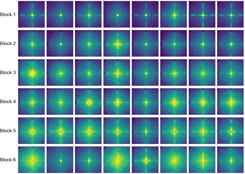
Figure II: Frequency magnitude ($14\times 14$) from 8 output channels of Hi-Fi in LITv2-S. The magnitude is averaged over 100 samples.

Figure III: Frequency magnitude ($14\times 14$) from 8 output channels of Lo-Fi in LITv2-S. The magnitude is averaged over 100 samples.

References

- [1] A. Ali, H. Touvron, M. Caron, P. Bojanowski, M. Douze, A. Joulin, I. Laptev, N. Neverova, G. Synnaeve, J. Verbeek, and H. Jégou. Xcit: Cross-covariance image transformers. In NIPS, pages 20014–20027, 2021.
- [2] J. Ba, J. Kiros, and G. E. Hinton. Layer normalization. ArXiv, abs/1607.06450, 2016.
- [3] B. Chen, P. Li, C. Li, B. Li, L. Bai, C. Lin, M. Sun, J. Yan, and W. Ouyang. Glit: Neural architecture search for global and local image transformer. In ICCV, 2021.
- [4] K. Chen, J. Wang, J. Pang, Y. Cao, Y. Xiong, X. Li, S. Sun, W. Feng, Z. Liu, J. Xu, Z. Zhang, D. Cheng, C. Zhu, T. Cheng, Q. Zhao, B. Li, X. Lu, R. Zhu, Y. Wu, J. Dai, J. Wang, J. Shi, W. Ouyang, C. C. Loy, and D. Lin. MMDetection: Open mmlab detection toolbox and benchmark. arXiv preprint arXiv:1906.07155, 2019.
- [5] M. Chen, H. Peng, J. Fu, and H. Ling. Autoformer: Searching transformers for visual recognition. In ICCV, pages 12250–12260, 2021.
- [6] Q. Chen, Q. Wu, J. Wang, Q. Hu, T. Hu, E. Ding, J. Cheng, and J. Wang. Mixformer: Mixing features across windows and dimensions. In CVPR, pages 5239–5249, 2022.
- [7] W. Chen, J. T. Wilson, S. Tyree, K. Q. Weinberger, and Y. Chen. Compressing convolutional neural networks in the frequency domain. In KDD, pages 1475–1484. ACM, 2016.
- [8] Y. Chen, X. Dai, D. Chen, M. Liu, X. Dong, L. Yuan, and Z. Liu. Mobile-former: Bridging mobilenet and transformer. In CVPR, pages 5260–5269, 2022.
- [9] Y. Chen, H. Fan, B. Xu, Z. Yan, Y. Kalantidis, M. Rohrbach, S. Yan, and J. Feng. Drop an octave: Reducing spatial redundancy in convolutional neural networks with octave convolution. In ICCV, pages 3434–3443. IEEE, 2019.
- [10] R. Child, S. Gray, A. Radford, and I. Sutskever. Generating long sequences with sparse transformers. arXiv preprint arXiv:1904.10509, 2019.
- [11] K. M. Choromanski, V. Likhosherstov, D. Dohan, X. Song, A. Gane, T. Sarlós, P. Hawkins, J. Q. Davis, A. Mohiuddin, L. Kaiser, D. B. Belanger, L. J. Colwell, and A. Weller. Rethinking attention with performers. In ICLR, 2021.
- [12] X. Chu, Z. Tian, Y. Wang, B. Zhang, H. Ren, X. Wei, H. Xia, and C. Shen. Twins: Revisiting the design of spatial attention in vision transformers. In NeurIPS, pages 9355–9366, 2021.
- [13] J. W. Cooley, P. A. W. Lewis, and P. D. Welch. The fast fourier transform and its applications. IEEE Transactions on Education, 12(1):27–34, 1969.
- [14] J. Cordonnier, A. Loukas, and M. Jaggi. On the relationship between self-attention and convolutional layers. In ICLR, 2020.
- [15] Z. Dai, H. Liu, Q. V. Le, and M. Tan. Coatnet: Marrying convolution and attention for all data sizes. In NeurIPS, pages 3965–3977, 2021.
- [16] G. Deng and L. Cahill. An adaptive gaussian filter for noise reduction and edge detection. In 1993 IEEE Conference Record Nuclear Science Symposium and Medical Imaging Conference, pages 1615–1619 vol.3, 1993.
- [17] X. Dong, J. Bao, D. Chen, W. Zhang, N. Yu, L. Yuan, D. Chen, and B. Guo. Cswin transformer: A general vision transformer backbone with cross-shaped windows. In CVPR, pages 12114–12124, 2022.
- [18] A. Dosovitskiy, L. Beyer, A. Kolesnikov, D. Weissenborn, X. Zhai, T. Unterthiner, M. Dehghani, M. Minderer, G. Heigold, S. Gelly, J. Uszkoreit, and N. Houlsby. An image is worth 16x16 words: Transformers for image recognition at scale. ICLR, 2021.
- [19] M. Fritsche, S. Gu, and R. Timofte. Frequency separation for real-world super-resolution. ICCVW, Oct 2019.
- [20] M.-H. Guo, C.-Z. Lu, Z.-N. Liu, M.-M. Cheng, and S.-M. Hu. Visual attention network. arXiv preprint arXiv:2202.09741, 2022.
- [21] K. Han, A. Xiao, E. Wu, J. Guo, C. Xu, and Y. Wang. Transformer in transformer. In NeurIPS, pages 15908–15919, 2021.
- [22] K. He, G. Gkioxari, P. Dollár, and R. B. Girshick. Mask R-CNN. In ICCV, pages 2980–2988, 2017.
- [23] K. He, X. Zhang, S. Ren, and J. Sun. Deep residual learning for image recognition. In CVPR, pages 770–778, 2016.
- [24] D. Hendrycks and K. Gimpel. Gaussian error linear units (gelus). arXiv preprint arXiv:1606.08415, 2016.
- [25] J. Huang, D. Guan, A. Xiao, and S. Lu. Rda: Robust domain adaptation via fourier adversarial attacking. In ICCV, pages 8988–8999, 2021.
- [26] Z. Huang, Y. Ben, G. Luo, P. Cheng, G. Yu, and B. Fu. Shuffle transformer: Rethinking spatial shuffle for vision transformer. arXiv preprint arXiv:2106.03650, 2021.
- [27] M. A. Islam, S. Jia, and N. D. B. Bruce. How much position information do convolutional neural networks encode? In ICLR, 2020.
- [28] A. Katharopoulos, A. Vyas, N. Pappas, and F. Fleuret. Transformers are rnns: Fast autoregressive transformers with linear attention. In ICML, pages 5156–5165. PMLR, 2020.
- [29] A. Kirillov, R. B. Girshick, K. He, and P. Dollár. Panoptic feature pyramid networks. In CVPR, pages 6399–6408, 2019.
- [30] T. Lin, P. Goyal, R. B. Girshick, K. He, and P. Dollár. Focal loss for dense object detection. In ICCV, pages 2999–3007, 2017.
- [31] T. Lin, M. Maire, S. J. Belongie, J. Hays, P. Perona, D. Ramanan, P. Dollár, and C. L. Zitnick. Microsoft COCO: common objects in context. In D. J. Fleet, T. Pajdla, B. Schiele, and T. Tuytelaars, editors, ECCV, pages 740–755, 2014.
- [32] Z. Liu, Y. Lin, Y. Cao, H. Hu, Y. Wei, Z. Zhang, S. Lin, and B. Guo. Swin transformer: Hierarchical vision transformer using shifted windows. In ICCV, pages 9992–10002, 2021.
- [33] Z. Liu, H. Mao, C.-Y. Wu, C. Feichtenhofer, T. Darrell, and S. Xie. A convnet for the 2020s. In CVPR, pages 11966–11976, 2022.
- [34] N. Ma, X. Zhang, H.-T. Zheng, and J. Sun. Shufflenet v2: Practical guidelines for efficient cnn architecture design. In ECCV, pages 116–131, 2018.
- [35] S. Mehta and M. Rastegari. Mobilevit: Light-weight, general-purpose, and mobile-friendly vision transformer. In ICLR, 2022.
- [36] Z. Pan, B. Zhuang, H. He, J. Liu, and J. Cai. Less is more: Pay less attention in vision transformers. In AAAI, pages 2035–2043, 2022.
- [37] Z. Pan, B. Zhuang, J. Liu, H. He, and J. Cai. Scalable visual transformers with hierarchical pooling. In ICCV, pages 377–386, 2021.
- [38] N. Park and S. Kim. How do vision transformers work? In ICLR, 2022.
- [39] H. Peng, N. Pappas, D. Yogatama, R. Schwartz, N. A. Smith, and L. Kong. Random feature attention. In ICLR, 2021.
- [40] J. W. Rae, A. Potapenko, S. M. Jayakumar, and T. P. Lillicrap. Compressive transformers for long-range sequence modelling. In ICLR, 2020.
- [41] Y. Rao, W. Zhao, Y. Tang, J. Zhou, S.-L. Lim, and J. Lu. Hornet: Efficient high-order spatial interactions with recursive gated convolutions. In NeurIPS, 2022.
- [42] Y. Rao, W. Zhao, Z. Zhu, J. Lu, and J. Zhou. Global filter networks for image classification. In NeurIPS, pages 980–993, 2021.
- [43] O. Russakovsky, J. Deng, H. Su, J. Krause, S. Satheesh, S. Ma, Z. Huang, A. Karpathy, A. Khosla, M. Bernstein, et al. Imagenet large scale visual recognition challenge. IJCV, pages 211–252, 2015.
- [44] S. Tang, J. Zhang, S. Zhu, and P. Tan. Quadtree attention for vision transformers. ICLR, 2022.
- [45] H. Touvron, M. Cord, M. Douze, F. Massa, A. Sablayrolles, and H. Jégou. Training data-efficient image transformers & distillation through attention. In ICML, pages 10347–10357, 2021.
- [46] H. Touvron, M. Cord, A. Sablayrolles, G. Synnaeve, and H. Jégou. Going deeper with image transformers. In ICCV, pages 32–42. IEEE, 2021.
- [47] Z. Tu, H. Talebi, H. Zhang, F. Yang, P. Milanfar, A. Bovik, and Y. Li. Maxim: Multi-axis mlp for image processing. CVPR, pages 5759–5770, 2022.
- [48] A. Vaswani, N. Shazeer, N. Parmar, J. Uszkoreit, L. Jones, A. N. Gomez, L. Kaiser, and I. Polosukhin. Attention is all you need. In NeurIPS, pages 5998–6008, 2017.
- [49] E. Voigtman and J. D. Winefordner. Low-pass filters for signal averaging. Review of Scientific Instruments, 57(5):957–966, 1986.
- [50] S. Wang, B. Li, M. Khabsa, H. Fang, and H. Ma. Linformer: Self-attention with linear complexity. arXiv preprint arXiv:2006.04768, 2020.
- [51] W. Wang, E. Xie, X. Li, D.-P. Fan, K. Song, D. Liang, T. Lu, P. Luo, and L. Shao. Pyramid vision transformer: A versatile backbone for dense prediction without convolutions. In ICCV, pages 548–558, 2021.
- [52] W. Wang, E. Xie, X. Li, D.-P. Fan, K. Song, D. Liang, T. Lu, P. Luo, and L. Shao. Pvtv2: Improved baselines with pyramid vision transformer. Computational Visual Media, 8(3):1–10, 2022.
- [53] R. Wightman, H. Touvron, and H. Jégou. Resnet strikes back: An improved training procedure in timm. CoRR, abs/2110.00476, 2021.
- [54] H. Wu, B. Xiao, N. Codella, M. Liu, X. Dai, L. Yuan, and L. Zhang. Cvt: Introducing convolutions to vision transformers. In ICCV, pages 22–31, 2021.
- [55] Z. Xia, X. Pan, S. Song, L. E. Li, and G. Huang. Vision transformer with deformable attention. In CVPR, pages 4794–4803, 2022.
- [56] M. Xiao, S. Zheng, C. Liu, Y. Wang, D. He, G. Ke, J. Bian, Z. Lin, and T. Liu. Invertible image rescaling. In ECCV, pages 126–144, 2020.
- [57] T. Xiao, M. Singh, E. Mintun, T. Darrell, P. Dollár, and R. B. Girshick. Early convolutions help transformers see better. In NeurIPS, pages 30392–30400, 2021.
- [58] S. Xie, R. B. Girshick, P. Dollár, Z. Tu, and K. He. Aggregated residual transformations for deep neural networks. In CVPR, pages 5987–5995, 2017.
- [59] K. Xu, M. Qin, F. Sun, Y. Wang, Y. Chen, and F. Ren. Learning in the frequency domain. In CVPR, pages 1737–1746. Computer Vision Foundation / IEEE, 2020.
- [60] J. Yang, C. Li, P. Zhang, X. Dai, B. Xiao, L. Yuan, and J. Gao. Focal self-attention for local-global interactions in vision transformers. In NeurIPS, pages 30008–30022, 2021.
- [61] K. Yuan, S. Guo, Z. Liu, A. Zhou, F. Yu, and W. Wu. Incorporating convolution designs into visual transformers. In ICCV, pages 559–568, 2021.
- [62] L. Yuan, Y. Chen, T. Wang, W. Yu, Y. Shi, F. E. Tay, J. Feng, and S. Yan. Tokens-to-token vit: Training vision transformers from scratch on imagenet. In ICCV, pages 538–547, 2021.
- [63] P. Zhang, X. Dai, J. Yang, B. Xiao, L. Yuan, L. Zhang, and J. Gao. Multi-scale vision longformer: A new vision transformer for high-resolution image encoding. In ICCV, pages 2978–2988, 2021.
- [64] Q. Zhang, Y. Xu, J. Zhang, and D. Tao. Vsa: Learning varied-size window attention in vision transformers. ECCV, 2022.
- [65] B. Zhou, H. Zhao, X. Puig, T. Xiao, S. Fidler, A. Barriuso, and A. Torralba. Semantic understanding of scenes through the ADE20K dataset. IJCV, pages 302–321, 2019.
- [66] Y. Zhou, W. Deng, T. Tong, and Q. Gao. Guided frequency separation network for real-world super-resolution. In CVPRW, pages 1722–1731, 2020.