Analyzing the Latent Space of GAN through Local Dimension Estimation

Abstract

The impressive success of style-based GANs (StyleGANs) in high-fidelity image synthesis has motivated research to understand the semantic properties of their latent spaces. In this paper, we approach this problem through a geometric analysis of latent spaces as a manifold. In particular, we propose a local dimension estimation algorithm for arbitrary intermediate layers in a pre-trained GAN model. The estimated local dimension is interpreted as the number of possible semantic variations from this latent variable. Moreover, this intrinsic dimension estimation enables unsupervised evaluation of disentanglement for a latent space. Our proposed metric, called Distortion, measures an inconsistency of intrinsic tangent space on the learned latent space. Distortion is purely geometric and does not require any additional attribute information. Nevertheless, Distortion shows a high correlation with the global-basis-compatibility and supervised disentanglement score. Our work is the first step towards selecting the most disentangled latent space among various latent spaces in a GAN without attribute labels.

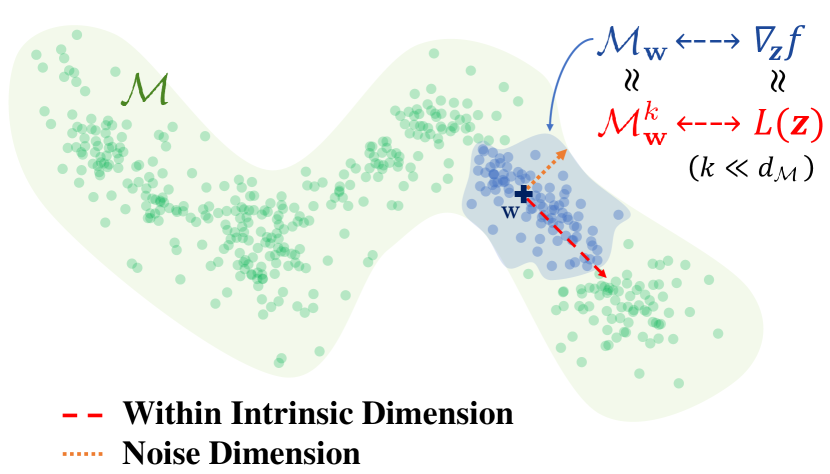
Figure 1: Local Dimension Estimation on Latent Manifold $\mathcal{M}$. Our goal is to find the dimension $k$ such that the $k$-dimensional submanifold $\mathcal{M}_{\mathbf{w}}^{k}$ represents the denoised local latent manifold $\mathcal{M}_{\mathbf{w}}\subseteq{\mathbb{R}}^{d_{\mathcal{M}}}$.

1 Introduction

Generative Adversarial Networks (GANs) (Goodfellow et al., 2014) have achieved remarkable success in generating realistic high-resolution images (Karras et al., 2018, 2019, 2020b, 2021, 2020a; Brock et al., 2018). Nevertheless, understanding how GAN models represent the semantics of images in their latent spaces is still a challenging problem. To this end, several recent works investigated the disentanglement (Bengio et al., 2013) properties of the latent space in GAN (Goetschalckx et al., 2019; Jahanian et al., 2019; Plumerault et al., 2020; Shen et al., 2020). A latent space is called disentangled if there is a bijective correspondence between each semantic attribute and each axis of latent space when represented with the optimal basis. (See the appendix for detail.) Due to this bijective correspondence, the disentangled latent space is a concise and interpretable representation of data (Bengio et al., 2013).

The style-based GAN models (Karras et al., 2019, 2020b) have been popular in previous studies for identifying a disentangled latent space in a pre-trained model. First, the space of style vector, called $\mathcal{W}$-space, was shown to provide a better disentanglement property compared to the latent noise space $\mathcal{Z}$ (Karras et al., 2019). After that, several attempts have been made to discover other disentangled latent spaces, such as $\mathcal{W}^{+}$-space (Abdal et al., 2019) and $\mathcal{S}$-space (Wu et al., 2020). However, the degree of disentanglement was assessed by the manual inspection (Karras et al., 2019; Abdal et al., 2019; Wu et al., 2020) or by the quantitative scores employing a pre-trained feature extractor (Karras et al., 2019) or an attribute annotator (Karras et al., 2019; Wu et al., 2020). The manual inspection is vulnerable to sample dependency, and the quantitative scores depend on the pre-trained models and the set of selected target attributes. Therefore, we need an unsupervised quantitative evaluation scheme for the disentanglement of latent space that does not rely on pre-trained models.

In this paper, we investigate the semantic property of a latent space in pre-trained GAN models by analyzing its geometrical property. Specifically, we propose a method for estimating the local (manifold) dimension of the learned latent space. Recently, Choi et al. (2022b) demonstrated that, in the learned latent space, the basis of tangent space describes the disentangled semantic variations. In this regard, the local intrinsic dimension represents the number of disentangled semantic variations from the given latent variable. Furthermore, this intrinsic dimension estimate leads to an unsupervised quantitative score for the disentanglement property of the latent space, called Distortion. Our experiments demonstrate that our proposed metric shows a high correlation with the global-basis-compatibility and supervised disentanglement score. (The global-basis-compatibility will be defined in Sec 4.) Our contributions can be summarized as follows:

1. We propose a local intrinsic dimension estimation scheme for an intermediate latent space in pre-trained GAN models. The estimated dimension and the corresponding refined latent manifold describe the principal variations of generated images.

2. We propose a layer-wise disentanglement score, called Distortion, that measures the inconsistency of intrinsic tangent space. The proposed metric shows a high correlation with the global-basis-compatibility and supervised disentanglement score.

3. We analyze the intermediate layers of the mapping network through Distortion metric. Our analysis elucidates the superior disentanglement of $\mathcal{W}$-space compared to the other intermediate layers and suggests a criterion for finding a similar-or-better alternative.

2 Related Works

Style-based Generator

Recently, GANs with style-based generator architecture (Karras et al., 2019, 2020b, 2021; Sauer et al., 2022) have achieved state-of-the-art performance in realistic image generation. In conventional GAN architecture, such as DCGAN (Radford et al., 2016) and ProGAN (Karras et al., 2018), the generator synthesizes an image by transforming a latent noise with a sequence of convolutional layers. On the other hand, the style-based generator consists of two subnetworks: mapping network $f:\mathcal{Z}\rightarrow\mathcal{W}$ and synthesis network $g:{\mathbb{R}}^{n_{0}}\times\mathcal{W}^{L}\rightarrow\mathcal{X}$. The synthesis network is similar to conventional generators in that it is composed of a series of convolutional layers $\{g_{i}\}_{i=1,\cdots,L}$. The key difference is that the synthesis network takes the learned constant feature $\mathbf{y}_{0}\in{\mathbb{R}}^{n_{0}}$ at the first layer $g_{0}$, and then adjusts the output image by injecting the layer-wise styles $\mathbf{w}$ and noise (Layer-wise noise is omitted for brevity.):

$$\mathbf{y}_{i}=g_{i}(\mathbf{y}_{i-1},\mathbf{w})\,\,\mathrm{with}\,\,\mathbf{w}=f(\mathbf{z})\,\,\mathrm{for}\,\,i=1,\cdots,L,$$ (1)

where the style vector $\mathbf{w}$ is attained by transforming a latent noise $\mathbf{z}$ via the mapping network $f$.

Understanding Latent Semantics

The previous attempts to understand the semantic property of latent spaces in StyleGANs are categorized into two topics: (i) finding more disentangled latent space in a model; (ii) discovering meaningful perturbation directions in a latent space corresponding to disentangled semantics. More precisely, the semantic perturbation in (ii) is defined as a latent perturbation that changes a generated image in only one semantics. Several studies on (i) suggested various disentangled latent spaces in StyleGAN models, for example, $\mathcal{W}$ (Karras et al., 2019), $\mathcal{W}^{+}$ (Abdal et al., 2019), $P_{N}$ (Zhu et al., 2020), and $\mathcal{S}$-space (Wu et al., 2020). However, the disentanglement of each latent space was compared by observing samples manually (Karras et al., 2019; Abdal et al., 2019; Wu et al., 2020) or by quantitative metrics relying on pre-trained models (Karras et al., 2019; Wu et al., 2020). Our Distortion metric achieves a high correlation with the supervised metric, e.g., DCI metric (Eastwood & Williams, 2018), while not requiring a pre-trained model.

Also, the previous works on (ii) are classified into local and global methods. The local methods find sample-wise perturbation directions (Ramesh et al., 2018; Patashnik et al., 2021; Abdal et al., 2021; Zhu et al., 2021; Choi et al., 2022b). On the other hand, the global methods search sample-independent perturbation directions that perform the same semantic manipulation on the entire latent space (Härkönen et al., 2020; Shen & Zhou, 2021; Voynov & Babenko, 2020). Throughout this paper, we refer to these local methods as local basis and these global methods as global basis. GANSpace (Härkönen et al., 2020) showed that the principal components obtained by PCA can serve as the global basis. SeFa (Shen & Zhou, 2021) suggested the singular vectors of the first weight parameter applied to latent noise as the global basis. These global basis showed promising results, but they were successful in a limited area. Depending on the sampled latent variables, these methods exhibited limited semantic factorization and sharp degradation of image fidelity (Choi et al., 2022b, a). In this regard, Choi et al. (2022b) suggested the need for diagnosing a global-basis-compatibility of latent space. If there is no ideal global basis for semantic attributes in the target latent space in the first place, all global basis can only attain limited success on it. Our Distortion metric can serve as a meaningful score for testing the global-basis-compatibility of latent spaces (Sec 4).

Semantic Analysis via Latent Manifold

Choi et al. (2022b) proposed an unsupervised method for finding local semantic perturbations based on the local geometry, called Local Basis (LB). Throughout this paper, we denote Local Basis as LB to avoid confusion with the general term ”local basis” in the previous paragraph. Assume the support $\mathcal{Z}$ of input prior distribution $p(\mathbf{z})$ is the entire Euclidean space, i.e., $\mathcal{Z}={\mathbb{R}}^{d_{\mathcal{Z}}}$, for example, Gaussian prior $p(\mathbf{z})=\mathcal{N}(0,I)$. We denote the target latent space by $\mathcal{M}=f(\mathcal{Z})\subseteq{\mathbb{R}}^{d_{\mathcal{M}}}$ and refer to the subnetwork between them by $f$. Note that $\mathcal{M}$ is defined as an image of the trained subnetwork $f$. Thus, we call $\mathcal{M}$ the learned latent space or latent manifold following the manifold interpretation of Choi et al. (2022b).

LB is defined as the ordered basis of tangent space $T_{\mathbf{w}}\mathcal{M}_{\mathbf{w}}^{k}$ at $\mathbf{w}=f(\mathbf{z})\in\mathcal{M}$ for the $k$-dimensional local approximating manifold $\mathcal{M}_{\mathbf{w}}^{k}$. Here, $\mathcal{M}_{\mathbf{w}}^{k}\subseteq\mathcal{M}$ indicates a $k$-dimensional submanifold of $\mathcal{M}$ that approximates $\mathcal{M}$ around $\mathbf{w}$ (Fig 1) with $k\leq d_{\mathcal{M}}$:

$$\mathcal{M}^{k}_{\mathbf{w}}\approx\mathcal{M}_{\mathbf{w}}\\ \textrm{where}\quad\mathcal{M}_{\mathbf{w}}=\left\{f\left(\mathbf{z}_{\epsilon}\right)\mid\|\mathbf{z}_{\epsilon}-\mathbf{z}\|<\epsilon\right\}\subseteq\mathcal{M}.$$ (2)

Using the fact that $\mathcal{M}=f(\mathcal{Z})$, the local approximating manifold $\mathcal{M}_{\mathbf{w}}^{k}$ can be discovered by solving the low-rank approximation problem of $df_{\mathbf{z}}$, i.e., the Jacobian matrix $\nabla_{\mathbf{z}}f$ of $f$ because of the assumption $T_{\mathbf{z}}\mathcal{Z}={\mathbb{R}}^{d_{\mathcal{Z}}}$:

$$\textrm{minimize}_{L}\,\,\|df_{\mathbf{z}}-L\|_{2},\quad\textrm{where}\,\,\operatorname{rank}(L)\leq k.$$ (3)

The analytic solution of this low-rank approximation problem is obtained in terms of Singular Value Decomposition (SVD) by Eckart–Young–Mirsky Theorem (Eckart & Young, 1936). From that, $\mathcal{M}_{\mathbf{w}}^{k}$ and the corresponding LB are given as follows: For the $i$-th singular vector $\mathbf{u}^{\mathbf{z}}_{i}\in{\mathbb{R}}^{d_{\mathcal{Z}}}$, $\mathbf{v}^{\mathbf{w}}_{i}\in{\mathbb{R}}^{d_{\mathcal{M}}}$, and $i$-th singular value $\sigma^{\mathbf{z}}_{i}\in{\mathbb{R}}$ of $df_{\mathbf{z}}$ with $\sigma^{\mathbf{z}}_{1}\geq\cdots\geq\sigma^{\mathbf{z}}_{n}$,

$$\text{(SVD) }\,\,df_{\mathbf{z}}(\mathbf{u}^{\mathbf{z}}_{i})=\sigma^{\mathbf{z}}_{i}\cdot\mathbf{v}^{\mathbf{w}}_{i}\quad\text{for}\,\,\forall i,$$ (4)

$$\text{LB}(\mathbf{w})=\{\mathbf{v}^{\mathbf{w}}_{i}\}_{1\leq i\leq n}\quad\text{where}\,\,\mathbf{w}=f(\mathbf{z}),$$ (5)

$$\mathcal{M}^{k}_{\mathbf{w}} =\left\{f\left(\mathbf{z}+\sum_{1\leq i\leq k}t_{i}\cdot\mathbf{u}^{\mathbf{z}}_{i}\right)\mid t_{i}\in(-\epsilon_{i},\epsilon_{i})\right\}.$$ (6)

Note that the tangent space of $\mathcal{M}_{\mathbf{w}}^{k}$ is spanned by the top-$\bm{k}$ LB, i.e. $T_{\mathbf{w}}\mathcal{M}^{k}_{\mathbf{w}}=\operatorname{span}\{\mathbf{v}^{\mathbf{w}}_{i}:1\leq i\leq k\}$. Choi et al. (2022b) demonstrated that LB serves as the local semantic perturbations from the base latent variable $\mathbf{w}$. However, estimating the number of meaningful perturbations remains elusive. Since LB is defined as singular vectors, LB presents the candidates as much as $\min(d_{\mathcal{Z}},d_{\mathcal{M}})$, e.g., 512 for $\mathcal{W}$-space in StyleGANs. To address this problem, we propose the local dimension estimation that can refine these candidates up to 90%. Moreover, this local dimension estimation leads to an unsupervised disentanglement metric (Sec 4).

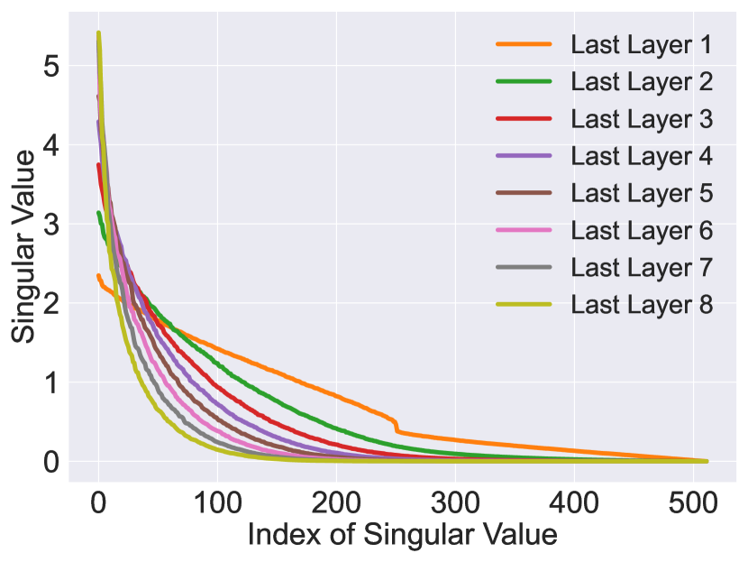
(a) Singular Value Distribution

(b) Off-manifold Results

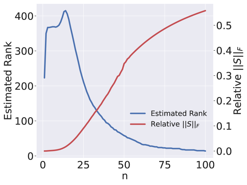
(c) Rank Estimation with Sparsity

Figure 2: (a) Singular Value Distribution of Jacobian matrix for each subnetwork of the mapping network in StyleGAN2. (b) Off-manifold Results in $\mathcal{W}$-space of StyleGAN2. (c) Rank Estimation with Sparsity under various $n=1/\gamma$.

3 Latent Dimension Estimation

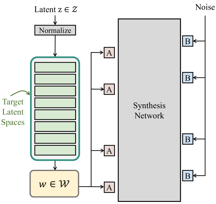
Figure 10: Architecture of StyleGANs. Our analysis in Sec 4 is performed in the intermediate layers of the mapping network.

In this section, we propose our local dimension estimation scheme for a learned latent manifold in a pre-trained GAN model. We interpret the latent manifold $\mathcal{M}=f(\mathcal{Z})$ as a noisy manifold, and hence the subnetwork differential $df_{\mathbf{z}}$ as a noisy linear map. The local dimension at $\mathbf{w}\in\mathcal{M}$ is estimated as the intrinsic rank of $df_{\mathbf{z}}$. Then, we evaluate the validity of this estimation scheme. In this section, our analysis of learned latent manifold is focused on the intermediate layers in the mapping network of StyleGAN2 trained on FFHQ (See Fig 10 for architecture). However, our scheme can be applied to any $\mathbf{z}$-differentiable intermediate layers for an input latent noise $\mathbf{z}$.

3.1 Method

Throughout this work, we follow the notation presented in Sec 2. Consider a target latent manifold $\mathcal{M}$ given by a subnetwork $f$, i.e., $\mathcal{M}=f(\mathcal{Z})$. Our goal is to estimate the intrinsic local dimension of $\mathcal{M}$ around $\mathbf{w}=f(\mathbf{z})$. Formally, the local dimension at $\mathbf{w}\in\mathcal{M}$ is the dimension of Euclidean space ${\mathbb{R}}^{k}$ whose open set is homeomorphic to the $\epsilon$-neighborhood of $\mathbf{w}$. However, the latent manifold exhibits some noise in practice. The bijective condition of homeomorphism is too strict under the presence of noise. Therefore, we define the local intrinsic dimension of learned latent space as the local dimension of denoised latent space (Fig 1). In particular, we discover this intrinsic dimension by estimating the intrinsic rank of noisy subnetwork differential $df_{\mathbf{z}}$, i.e., the Jacobian $(\nabla_{\mathbf{z}}f)(\mathbf{z})$. The correspondence between the local dimension and rank of $df_{\mathbf{z}}$ is described in Eq 6 because the rank of a linear map is the same as the number of singular vectors with non-zero singular values.

Motivation

Before presenting our dimension estimation method, we provide motivation for introducing the lower-dimensional approximation to $\mathcal{M}$. Figure 2(a) shows the singular value distribution of Jacobian matrices evaluated for the subnetworks of the mapping network in StyleGAN2. Last layer $i$ denotes the subnetwork from the input noise space $\mathcal{Z}$ to the $i$-th fully connected layer. The distribution of singular values $\{\sigma_{i}^{\mathbf{z}}\}_{i}$ gets monotonically sparser as the subnetwork gets deeper. In particular, $\mathcal{W}$-space, i.e., Last layer 8, is extremely sparse as much as $\sigma_{150}^{\mathbf{z}}/\sigma_{1}^{\mathbf{z}}\approx 0.005$. Therefore, it is reasonable to prune the singular values with negligible magnitude and consider the lower-dimensional approximation of the learned latent manifold.

Local Dimension Estimation

Our intrinsic rank estimation algorithm distinguishes the large meaningful components and the small noise-like components given the singular values $\{\sigma_{i}^{\mathbf{z}}\}_{i}$ of $(\nabla_{\mathbf{z}}f)(\mathbf{z})$. The Pseudorank algorithm (Kritchman & Nadler, 2008) estimates the number of meaningful components in a linear mixture model from noisy samples. We reinterpret this algorithm to find the intrinsic rank of noisy $(\nabla_{\mathbf{z}}f)(\mathbf{z})$. Assume the isotropic Gaussian noise on the Jacobian $(\nabla_{\mathbf{z}}f)(\mathbf{z})\in{\mathbb{R}}^{d_{\mathcal{M}}\times d_{\mathcal{Z}}}$:

$$(\nabla_{\mathbf{z}}f)(\mathbf{z})=L(\mathbf{z})+\sigma\cdot\left(\epsilon_{1},\cdots,\epsilon_{d_{\mathcal{M}}}\right)^{\intercal},$$ (7)

with $\epsilon_{i}\sim\mathcal{N}(0,I_{d_{\mathcal{Z}}})$ where $L(\mathbf{z})$ denotes the denoised low-rank representation of $(\nabla_{\mathbf{z}}f)(\mathbf{z})$. Then, taking the expectation over the noise distribution gives:

$$\mathbb{E}_{\epsilon}\left[(\nabla_{\mathbf{z}}f)^{\intercal}(\mathbf{z})\cdot(\nabla_{\mathbf{z}}f)(\mathbf{z})\right]=L^{\intercal}(\mathbf{z})\cdot L(\mathbf{z})+\sigma^{2}\cdot I_{d_{\mathcal{Z}}}.$$ (8)

The eigenvalues of $\left[(\nabla_{\mathbf{z}}f)^{\intercal}(\mathbf{z})\cdot(\nabla_{\mathbf{z}}f)(\mathbf{z})\right]$ are the squares of sigular values $\{(\sigma_{i}^{\mathbf{z}})^{2}\}_{i}$, and the noise covariance term $\sigma^{2}\cdot I_{d_{\mathcal{Z}}}$ increases all eigenvalues by $\sigma^{2}$. This observation explains our intuition that large singular values correspond to signals and small ones correspond to noise. Therefore, determining the intrinsic rank of $(\nabla_{\mathbf{z}})f(\mathbf{z})$ is closely related to the largest eigenvalue $\lambda_{1}$ of the empirical covariance matrix $S=\frac{1}{d_{\mathcal{Z}}}\sum_{i}\epsilon_{i}\cdot\epsilon_{i}^{\intercal}$, which is the threshold for distinguishing between signal and noise. In the random matrix theory, it is known that the distribution of this largest eigenvalue $\lambda_{1}$ for $n$-samples of $\mathcal{N}(0,I_{p})$ converges to a Tracy-Widom distribution $F_{\beta}$ of order $\beta=1$ for real-valued observations (Johnstone, 2001) (See the appendix for detail.):

$$P\left(\lambda_{1}<\sigma^{2}\left(\mu_{n,p}+s\cdot\sigma_{n,p}\right)\right)\rightarrow F_{\beta}(s)\\ \textrm{as $n,p\rightarrow\infty$ with $c=p/n$ fixed.}$$ (9)

Using the above theoretical results, our algorithm applies a sequence of nested hypothesis tests. Given the Jacobian $(\nabla_{\mathbf{z}}f)(\mathbf{z})\in{\mathbb{R}}^{d_{\mathcal{M}}\times d_{\mathcal{Z}}}$, let $p=\min(d_{\mathcal{M}},d_{\mathcal{Z}})$. Then, for $k=1,2,\cdots,p-1$,

$$\mathcal{H}_{0}:\textrm{rank at least }k\,\,\,\text{vs.}\,\,\,\mathcal{H}_{1}:\textrm{rank at most }(k-1)$$ (10)

For each $k$, the hypothesis test consists of two parts. First, the noise level $\sigma$ of $(\nabla_{\mathbf{z}}f)(\mathbf{z})$ in Eq 7 should be estimated to perform a hypothesis test. We adopted the consistent noise estimate $\sigma_{est}(k)$ from Kritchman & Nadler (2008), which is derived by assuming that $\lambda_{k+1},\lambda_{k+2}\cdots,\lambda_{p}$ are the noise components for $\lambda_{i}=(\sigma_{i}^{\mathbf{z}})^{2}$. Second, we test whether $\lambda_{k}$ belongs to the noise components based on the corresponding Tracy-Widom distribution as follows:

$$\lambda_{k}\leq\sigma_{est}^{2}(k)\left(\mu_{n,p-k}+s(\alpha)\cdot\sigma_{n,p-k}\right),$$ (11)

where $\alpha$ denotes a confidence level. We chose $\alpha=0.1$ in our experiments. The above test is repeated until Eq 11 is satisfied. Then, the estimated rank $K$ becomes $K=k-1$ because Eq 11 means that $\lambda_{k}$ is not large enough to be judged as a signal component.

(a) $\theta_{pre}=0.001$

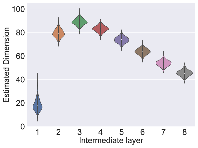
(b) $\theta_{pre}=0.005$

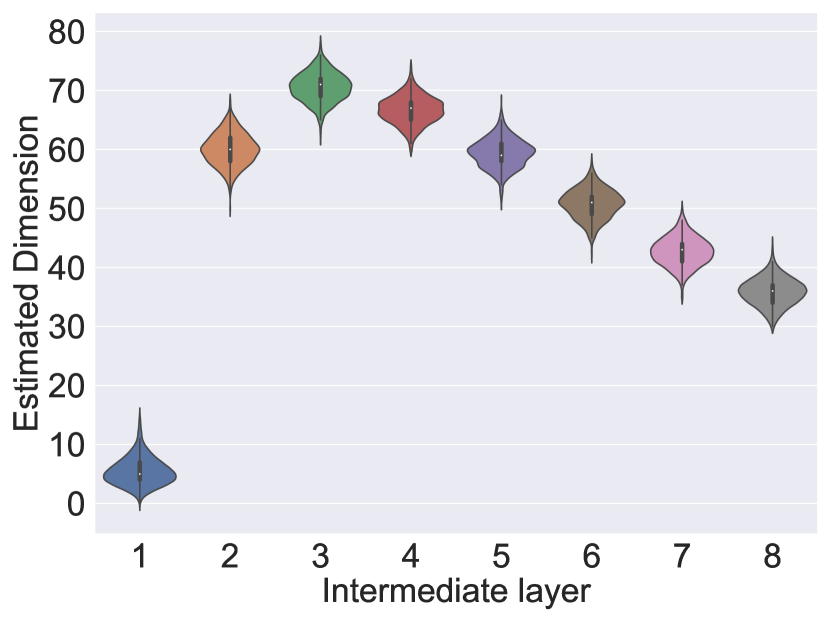
(c) $\theta_{pre}=0.01$

Figure 3: Local Dimension Distribution of the intermediate layers in the mapping network.

Preprocessing

This algorithm supposes the isotropic Gaussian noise on the Jacobian matrix. However, even considering the randomness of empirical covariance, the observed singular values of Jacobian matrix are too sparse ($\sigma_{min}/\sigma_{max}\approx 10^{-9}$). Hence, the isotropic Gaussian assumption leads to the underestimation of the noise level, which causes the overestimation of intrinsic rank (In our experiments, estimated rank $>200$ and $\sigma_{rank}\approx 0.003$). To address this problem, we introduce a simple preprocessing on the singular values of the Jacobian. Before applying the rank estimation algorithm, we filter out the singular values $\{\sigma_{i}^{\mathbf{z}}\}_{i}$ with $\{(\sigma_{i}^{\mathbf{z}})^{2}\leq\theta_{pre}\cdot\max_{i}(\sigma_{i}^{\mathbf{z}})^{2}\}$. We set $\theta_{pre}\in\{0.0005,0.001,0.005,0.01\}$.

Validity of the estimated local dimension

Our local dimension estimate is based on the Jacobian $\nabla_{\mathbf{z}}f$, where $f$ defines the latent manifold $\mathcal{M}=f(\mathcal{Z})$. Because $\nabla_{\mathbf{z}}f$ is the first order approximation of $f$, the estimated dimension might be improper for $\mathcal{M}$. Therefore, we designed and conducted the Off-manifold experiment to assess the validity of the estimated local dimension. Intuitively, the intrinsic local dimension at $\mathbf{w}\in\mathcal{M}$ is discovered by refining minor variations of the noisy latent manifold. The goal of Off-manifold experiment is to test whether the latent perturbation along the $k$-th coordinate axis stays inside $\mathcal{M}$. If the margin of $\mathcal{M}$ at $\mathbf{w}$ in the $k$-th axis is large enough, then the $k$-th axis is needed to locally approximate $\mathcal{M}$. To be more specific, we solve the following optimization problem by Adam optimizer (Kingma & Ba, 2015) on MSE loss with a learning rate 0.005 for 1000 iterations for each $k$ with $\mathbf{z}_{0}=\mathbf{z}_{init}$:

$$\mathbf{w}_{init}=f(\mathbf{z}_{init}),\quad\mathbf{w}_{ptb}=\mathbf{w}_{init}+c\cdot\mathbf{v}^{\mathbf{w}_{init}}_{k},$$ (12)

$$\mathbf{z}_{opt}=\arg\min_{\mathbf{z}}\|\mathbf{w}_{ptb}-f(\mathbf{z})\|^{2}.$$ (13)

Here, $\mathbf{v}^{\mathbf{w}_{init}}_{k}$ denotes the $k$-th LB at $\mathbf{w}_{init}$. $\mathbf{w}_{init}$ is perturbed along $\mathbf{v}^{\mathbf{w}_{init}}_{k}$ because it is the tangent vector at $\mathbf{w}_{init}$ along $k$-th axis (Eq 4).

We ran the Off-manifold experiments on $\mathcal{W}$-space of StyleGAN2. Figure 2(b) shows the final objective $\|\mathbf{w}_{ptb}-f(\mathbf{z}_{opt})\|^{2}$ after the optimization for each LB $\mathbf{v}^{\mathbf{w}_{init}}_{k}$ with $c=2$. The red vertical lines denote the estimated local dimension for each $\theta_{pre}$. (See the appendix for the Off-manifold results with various $c=\|\mathbf{w}_{ptb}-\mathbf{w}_{init}\|$.) The monotonous increase in the final loss shows that $f(\mathbf{z}_{opt})$ cannot approach close to $\mathbf{w}_{ptb}$. In other words, the margin in the $k$-th LB direction decreases as the index $k$ increases. Although there is a dependency on the preprocessing threshold, the rank estimation algorithm chooses the principal part of local manifold around $\mathbf{w}_{init}$ without overestimates as desired. Particularly, the estimated rank with $\theta_{pre}=0.005$ appears to find a transition point of the final loss.

(a) Image Traversal along Axis 0 and 1

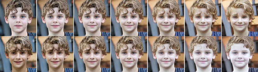
(b) Image Traversal along Axis $(d-1)$ and $d$

(c) Image Variation along Singular Vectors

Figure 4: Local Dimension Evaluation in Image Space where $d$ denotes the estimated local dimension with $\theta_{pre}=0.01$. Fig 4(c) shows the image variation intensity $\|\nabla_{\mathbf{v}_{i}^{\mathbf{w}}}g(\mathbf{w})\|_{F}$ along each LB $\mathbf{v}_{i}$.

3.2 Comparison to Previous Rank Estimation

Sparsity Constraint

LowRankGAN (Zhu et al., 2021) introduced a convex optimization problem called Principal Component Pursuit (PCP) (Candès et al., 2011) to find a low-rank factorization of Jacobian $(\nabla_{\mathbf{z}}f)(\mathbf{z})$ (Eq 14):

$$\textrm{min}_{L,S}\quad\|L\|_{*}+\gamma\cdot\|S\|_{1}\\ \textrm{s.t.}\,\,L+S=(\nabla_{\mathbf{z}}f)^{\intercal}(\mathbf{z})\cdot(\nabla_{\mathbf{z}}f)(\mathbf{z}).$$ (14)

where $\|L\|_{*}=\sum_{i}\sigma_{i}(L)$ is the nuclear norm, i.e. the sum of all singular values, $\|S\|_{1}=\sum_{i,j}|S_{i,j}|$, and $\gamma>0$ is a positive regularization parameter. PCP encourages the sparsity on corruption $S$ through $\ell_{1}$ regularizer.

However, we believe that this sparsity assumption is not adequate for finding the intrinsic rank of Jacobian. To test the validity of the sparsity assumption, we monitored how the low-rank representation $L$ changes as we vary the regularization parameter $n=1/\gamma$ as in (Zhu et al., 2021) (Fig 2(c)). The estimated rank decreases unceasingly without saturation as we increase $n$, i.e., refine the Jacobian stronger. We consider that the rank saturation should occur if this assumption is adequate for finding an intrinsic rank because it implies regularization robustness. But the low-rank factorization through PCP does not show any saturation until the Frobenius norm of corruption $\|S\|_{F}$ reaches over 50$\%$ of the initial matrix $\|(\nabla_{\mathbf{z}}f)^{\intercal}(\mathbf{z})\cdot(\nabla_{\mathbf{z}}f)(\mathbf{z})\|_{F}$.

Interpretation as Frobenious Norm

Our algorithm can be interpreted as a Nuclear-Norm Penalization (NNP) problem (Eq 15) for matrix denoising (Donoho & Gavish, 2014). This NNP framework is similar to PCP in LowRankGAN except for the regularization $\|E\|_{F}$. While PCP requires an iterative optimization of Alternating Directions Method of Multipliers (ADMM) (Boyd et al., 2011; Lin et al., 2010), NNP provides an explicit closed-form solution $L^{*}$ through SVD, i.e., $(\nabla_{\mathbf{z}}f)(\mathbf{z})=U\Sigma V^{\intercal}$:

$$\textrm{min}_{L,S}\,\,\|L\|_{*}+\gamma\|E\|_{F}\quad\textrm{s.t.}\,\,L+E=(\nabla_{\mathbf{z}}f)(\mathbf{z}).$$ (15)

$$\Rightarrow L^{*}=U\left(\Sigma-\frac{1}{2\gamma}\cdot I\right)_{+}V^{\intercal}$$ (16)

for $(M_{+})_{i,j}=\max\left(M_{i,j}\,,0\right)$. Therefore, the intrinsic rank by NNP is determined by a threshold $1/(2\gamma)$ for the singular values $\{\sigma_{i}^{\mathbf{z}}\}_{i}$ of Jacobian. Our algorithm can be interpreted as selecting this threshold via a series of hypothesis tests.

3.3 Latent Space Analysis of StyleGAN

We analyzed the intermediate layers of the mapping network in StyleGAN2 trained on FFHQ using our local dimension estimation (See Fig 10 for StyleGAN architectures). First, Figure 3 shows the distribution of estimated local dimensions for 1k samples of each intermediate layer for each $\theta_{pre}$ (See the appendix for the rank statistics under all $\theta_{pre}$). Note that the algorithm provides an unstable rank estimate on the most unsparse $1$st layer (Fig 2(a)) under the small $\theta_{pre}\in\{0.0005,0.001\}$. However, this phenomenon was not observed in the other layers. Hence, we focused our analysis on the layers with reasonable depth, i.e., from $3$ to $8$. Even though changing $\theta_{pre}$ results in an overall shift of the estimation, the trend and relative ordering between layers are the same. In accordance with Fig 2(a), the intrinsic dimension monotonically decrease as the layer goes deeper.

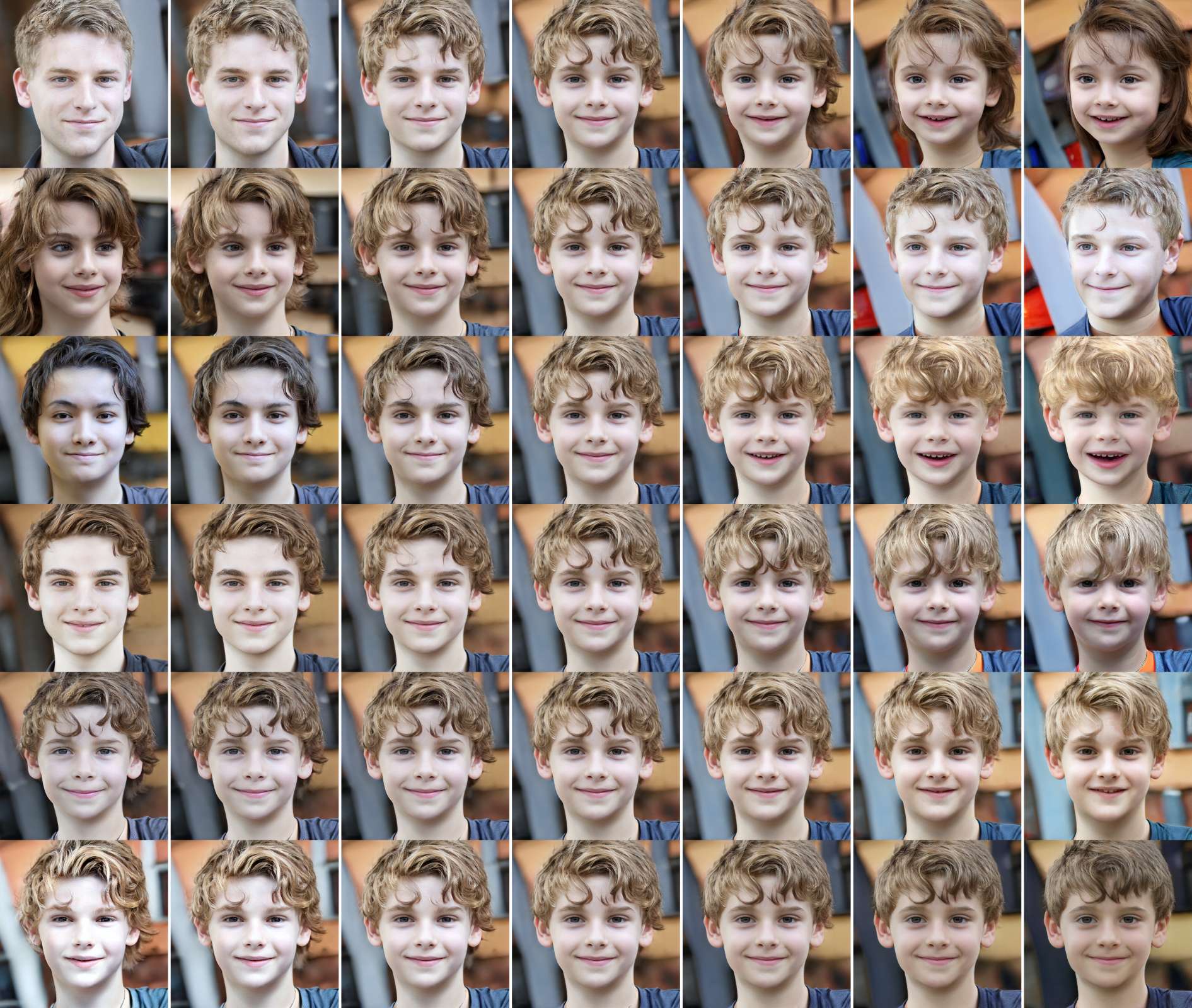
(a) Axes $\{0,1,15,30,43,44\}$ from top to bottom

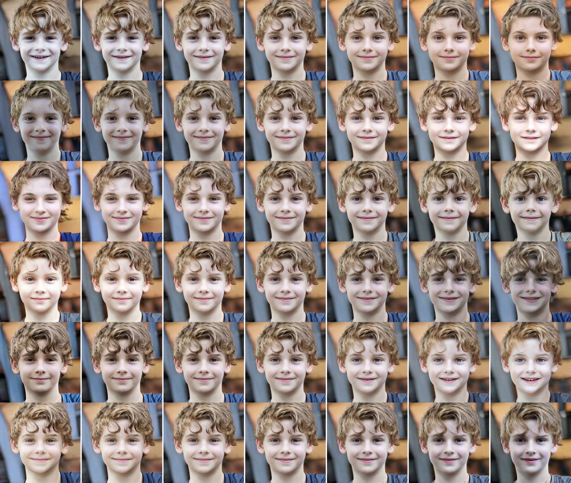
(b) Axes $\{100,150,200,300,400,500\}$

Figure 22: Linear Traversals along the various LB axis on StyleGAN2-FFHQ. At this latent variable, the estimated dimension with $\theta_{pre}=0.01$ is $d=44$. When we traverse along the axis $i\gg d$, the images present minor variations compared to the axis $i\leq d$. Traversals along the 1 - 44 axes display various semantic variations such as gender, skin color, age, etc.

Second, we evaluated the estimated rank on image space (Fig 4). Figure 4(a) and 4(b) show the image traversal along the first two axes and the two axes $(d-1,d)$ around the estimated rank $d$ with $\theta_{pre}=0.01$ (See Fig 22 for comparison between axis $i<d$ and $i\gg d$.) Fig 4(c) presents the size of the directional derivative $\|\nabla_{\mathbf{v}_{i}^{\mathbf{w}}}g(\mathbf{w})\|_{F}$ along the $i$-th LB $\mathbf{v}_{i}^{\mathbf{w}}$ at $\mathbf{w}$, estimated by the finite difference scheme. The result shows that the estimated rank covers the major variations in the image space. Choi et al. (2022b) proposed LB as the unsupervised local basis for the latent space in GANs, but did not provide an estimate on the number of meaningful perturbations. One advantage of the unsupervised method over the supervised one for finding disentangled perturbation is that the discovered semantic is not restricted to pre-defined attributes. However, we cannot know the number of meaningful perturbations without additional inspections. Figure 4 shows that the estimated dimension provides an upper bound on the number of these perturbations.

(a) StyleGAN2-Cat - $\rho=0.98$

(b) StyleGAN2-e - $\rho=0.81$

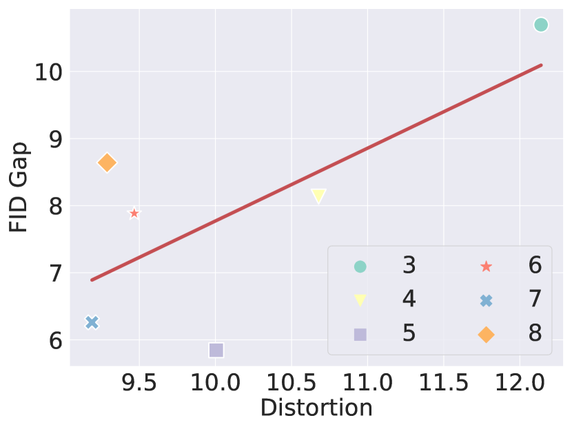
(c) StyleGAN2 - $\rho=0.70$

Figure 5: Correlation between Distortion metric ($\downarrow$) and FID gap ($\downarrow$) when $\theta_{pre}=0.005$. FID gap represents the difference between FID score of LB and GANSpace. Each point represents a $i$-th intermediate layer in the mapping network.

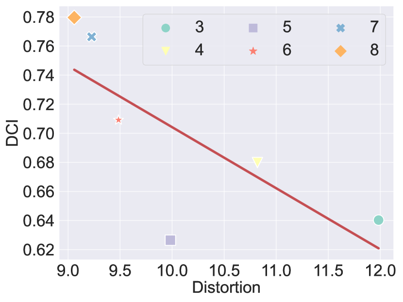
(a) StyleGAN1 - $\rho=-0.74$

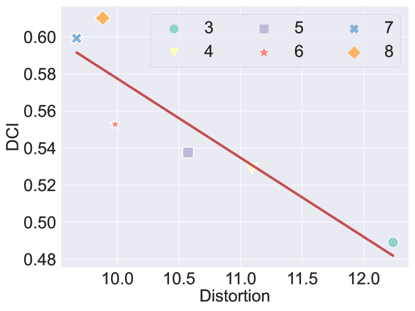
(b) StyleGAN2-e - $\rho=-0.91$

(c) StyleGAN2 - $\rho=-0.57$

Figure 6: Correlation between Distortion metric ($\downarrow$) and DCI ($\uparrow$) when $\theta_{pre}=0.005$. DCI (Eastwood & Williams, 2018) is a supervised disentanglement metric that requires attribute annotations.

4 Unsupervised Global Disentanglement Evaluation

In this section, we investigate two closely related important questions on the disentanglement property of a GAN.

1. Can we evaluate the global-basis-compatibility of the latent space without posterior assessment? (Choi et al., 2022b)

2. Can we evaluate the disentanglement without attribute annotations? (Locatello et al., 2019)

Here, the global-basis-compatibility represents the representability upper-bound of latent space that the optimal global basis can achieve. If a latent space has a low global-basis-compatibility, all global basis can attain constrained success on it.

These two questions are closely related because the ideal disentanglement includes a global basis representation where each element corresponds to the attribute-coordinate. In this paper, the global disentanglement property of a latent space is defined as this global representability along the attribute-coordinate. To answer these questions, we propose an unsupervised global disentanglement metric, called Distortion. We evaluate the global-basis-compatibility by the image fidelity (Q1) and the disentanglement by semantic factorization (Q2). Our experimental results show that our proposed metric achieves a high correlation with the global-basis-compatibility (Q1) and the supervised disentanglement score (Q2) on various StyleGANs. (See Fig 9 in appendix for robustness of Distortion to $\theta_{pre}$.)

Distortion Score

Intuitively, our global disentanglement score assesses the inconsistency of intrinsic tangent space for each latent manifold. The framework of analyzing the semantic property of a latent space via its tangent space was first introduced in Choi et al. (2022b). This framework was inspired by the observation that each basis vector (LB) of a tangent space corresponds to a local semantic perturbation. In this work, we develop this idea and propose a layer-wise score for global disentanglement property. As in Choi et al. (2022b), we employ the Grassmannian (Boothby, 1986) metric to measure a distance between two tangent spaces. We chose the Geodesic Metric (Ye & Lim, 2016) instead of the Projection Metric (Karrasch, 2017) because of its better discriminability (See Sec D for detail). Also, we revised the Geodesic Metric to be dimension-normalized because the local dimension changes according to its estimated region.

For two $k$-dimensional subspaces $W,W^{\prime}$ of ${\mathbb{R}}^{n}$, let $M_{W},M_{W^{\prime}}\in{\mathbb{R}}^{n\times k}$ be the column-wise concatenation of orthonormal basis for $W,W^{\prime}$, respectively. Then, the dimension-normalized Geodesic Metric is defined as $d^{k}_{\mathrm{geo}}(W,W^{\prime})=\left(\frac{1}{k}\sum^{k}_{i=1}\theta^{2}_{i}\right)^{1/2}$ where $\theta_{i}=\cos^{-1}(\sigma_{i}(M_{W}^{\top}\,M_{W^{\prime}}))$ denotes the $i$-th principal angle between $W$ and $W^{\prime}$ for $i$-th singular value $\sigma_{i}$. Then, Distortion score $\mathcal{D}_{\mathcal{M}}$ for the latent manifold $\mathcal{M}$ is evaluated as follows:

1. To assess the overall inconsistency of $\mathcal{M}$, measure the Grassmannian distance between two intrinsic tangent spaces $T_{\mathbf{w}_{i}}\mathcal{M}^{k_{i}}_{\mathbf{w}_{i}}$ (Eq 6) at two random $\mathbf{w}\in\mathcal{M}$. For $k=\min(k_{1},k_{2})$,

   $$I_{rand}=\mathbb{E}_{\begin{subarray}{c}\mathbf{z}_{i}\sim p(\mathbf{z}),\\ \mathbf{w}_{i}=f(\mathbf{z}_{i})\end{subarray}}\left[d^{k}_{\mathrm{geo}}\left(\,T_{\mathbf{w}_{1}}\mathcal{M}^{k}_{\mathbf{w}_{1}},T_{\mathbf{w}_{2}}\mathcal{M}^{k}_{\mathbf{w}_{2}}\right)\right].$$

2. To normalize the overall inconsistency, measure the same Grassmannian distance between two close $\mathbf{w}\in\mathcal{M}$ for $\epsilon=0.1$

   $$I_{local}=\mathbb{E}_{\begin{subarray}{c}\mathbf{z}_{1}\sim p(\mathbf{z}),\\ |\mathbf{z}_{2}-\mathbf{z}_{1}|=\epsilon\end{subarray}}\left[d^{k}_{\mathrm{geo}}\left(\,T_{\mathbf{w}_{1}}\mathcal{M}^{k}_{\mathbf{w}_{1}},T_{\mathbf{w}_{2}}\mathcal{M}^{k}_{\mathbf{w}_{2}}\right)\right].$$

3. Distortion of $\mathcal{M}$ is defined as the relative inconsistency $\mathcal{D}_{\mathcal{M}}=I_{rand}/I_{local}$.

Distortion and Global Disentanglement

In this paragraph, we clarify why the globally disentangled latent space shows a low Distortion score. Assume a latent space $\mathcal{M}$ is globally disentangled. Then, there exists an optimal global basis of $\mathcal{M}$, where each basis vector corresponds to an image attribute on the entire $\mathcal{M}$. By definition, this optimal global basis is the local basis at all latent variables. Assuming that LB finds the local basis (Choi et al., 2022b), each global basis vector would correspond to one LB vector at each latent variable. In this regard, our local dimension estimation finds a principal subset of LB, which includes these corresponding basis vectors. In conclusion, if the latent space is globally disentangled, this principal set of LB at each latent variable would contain the common global basis vectors. Hence, the intrinsic tangent spaces would contain the common subspace generated by this common basis, which leads to a small Grassmannian metric between them. Therefore, the global disentanglement of the latent space leads to a low Distortion score.

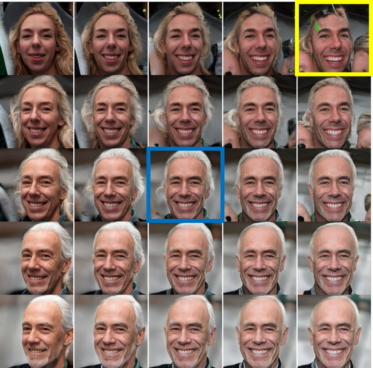
(a) Max-distorted layer 3

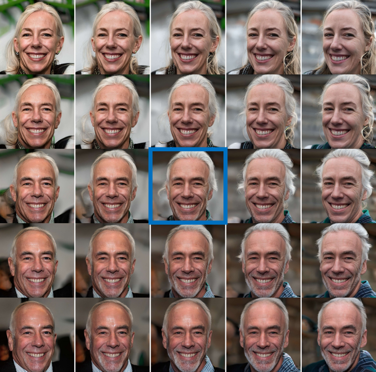
(b) Min-distorted layer 7

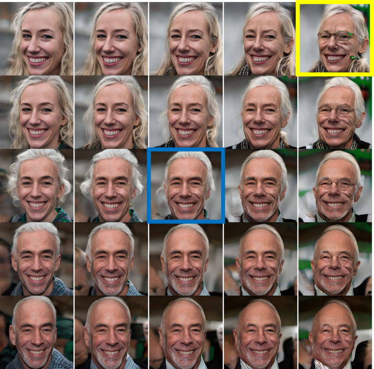
(c) Layer 8 ($\mathcal{W}$-space)

Figure 7: Subspace Traversal on the intermediate layers along the global basis. The upper-right corner of max-distorted layer 3 and layer 8 show visual artifacts. However, the min-distorted layer 7 does not show such a failure. The initial image (center) is traversed along the $1$st (horizontal) and $2$nd (vertical) components of GANSpace with a perturbation intensity 4.

Global-Basis-Compatibility

We tested whether Distortion $\mathcal{D}_{\mathcal{M}}$ is meaningful in estimating the global-basis-compatibility. We chose GANSpace (Härkönen et al., 2020) as a reference global basis because of its broad applicability. As a measure of global-basis-compatibility, we adopted FID (Heusel et al., 2017) gap between LB and GANSpace. Here, we interpret FID score under LB traversal as the optimal image fidelity that the latent space can achieve because LB is the basis of tangent space. Thus, FID gap between LB and GANSpace represents the difference between the optimal image fidelity and the fidelity achieved by a global basis. Therefore, we selected this FID gap for assessing the global-basis-compatibility. FID is measured for 50k samples of perturbed images along the 1st component of LB and GANSpace, respectively. Distortion metric is tested on StyleGAN2 on LSUN Cat, StyleGAN2 with configs E and F (Karras et al., 2020b) on FFHQ to test the generalizability of correlation to the global-basis-compatibility. StyleGAN2 in Fig 5 denotes StyleGAN2 with config F because config F is the usual StyleGAN2 model. The perturbation intensity is set to 5 in LSUN Cat and 3 in FFHQ. Distortion metric shows a strong positive correlation of 0.98, 0.81 and 0.70 to FID gap in Fig 5. (See Sec G for correlations on other $\theta_{pre}$.) This result demonstrates that Distortion metric can be an unsupervised criterion for selecting a latent space with high global-basis-compatibility. This suggests that, before finding a global basis, we can use Distortion metric as a prior investigation for selecting a proper target latent space.

Disentanglement Score

We assessed a correlation between the unsupervised Distortion metric and a supervised disentanglement score. Following Wu et al. (2020), we adopted DCI score (Eastwood & Williams, 2018) as the supervised disentanglement score for evaluation, and employed 40 binary attribute classifiers pre-trained on CelebA (Liu et al., 2015) to label generated images. Each DCI score is assessed on 10k samples of latent variables with the corresponding attribute labels. In Fig 6, StyleGAN1, StyleGAN2-e, and StyleGAN2 refer to StyleGAN1 and StyleGAN2s with config E and F trained on FFHQ. Note that DCI experiments are all performed on FFHQ because the DCI score requires attribute annotations. DCI and Distortion metrics show a strong negative correlation on StyleGAN1 and StyleGAN2-e. The correlation is relatively moderate on StyleGAN2. This moderate correlation is because Distortion metric is based on the Grassmannian metric. The Grassmannian metric measures the distance between tangent spaces, while DCI is based on their specific basis. Even if the tangent space is identical so that Distortion becomes zero, DCI can have a relatively low value depending on the choice of basis. Hence, in StyleGAN2, the high-distorted layers showed low DCI scores, but the low-distorted layers showed relatively high variance in DCI score. Nevertheless, the strong correlation observed in the other two experiments suggests that, in practice, the basis vector corresponding to a specific attribute has a limited variance in a given latent space. Therefore, Distortion metric can be an unsupervised indicator for the supervised disentanglement score.

Traversal Comparison

In all StyleGAN models, layer 7 and layer 8 ($\mathcal{W}$-space) achieved the smallest Distortion metric (Fig 5 and 6). These results explain the superior disentanglement of renowned $\mathcal{W}$-space. Moreover, our Distortion suggests that layer 7 can be an alternative to $\mathcal{W}$-space. Our global-basis-compatibility results imply that the min-distorted layer can present better image fidelity under the global basis traversal. For a visual comparison, we observed the subspace traversal (Choi et al., 2022b) along the global basis on the max-distorted layer 3, min-distorted layer 7, and $\mathcal{W}$-space of StyleGAN2 on FFHQ. The subspace traversal visualizes the two-dimensional latent perturbation. Hence, the subspace traversal can reveal the deviation from the tangent space more clearly than the linear traversal, because the deviation is assessed in two dimensions. Note that the tangent space is the optimal perturbation in image fidelity. In Fig 7, the global basis shows visual artifacts at the corners in the subspace traversal on the max-distorted layer 3 and $\mathcal{W}$-space. Nevertheless, the min-distorted layer 7 shows the stable traversal without any failure. This result proves that comparing Distortion scores can be a criterion for selecting a better latent space with higher global-basis-compatibility. (See Sec J for additional image fidelity comparisons and Sec I for semantic factorization comparisons.)

5 Conclusion

In this paper, we proposed a local intrinsic dimension estimation algorithm for the intermediate latent space in a pre-trained GAN. Using this algorithm, we analyzed the intermediate layers in the mapping network of StyleGANs on various datasets. Moreover, we suggested an unsupervised global disentanglement metric called Distortion. The analysis of the mapping network demonstrates that Distortion metric shows a high correlation between the global-basis-compatibility and disentanglement score. Although finding an optimal preprocessing hyperparameter $\theta_{pre}$ was beyond the scope of this work, the proposed metric showed robustness to the hyperparameter. Moreover, our local dimension estimation has the potential to be applied to feature spaces of various models. This kind of research would be an interesting future work.

Appendix A Definition of disentangled latent space

Disentangled perturbation

In the GAN disentanglement literature, several studies investigated the disentanglement property of the latent space by finding disentangled perturbations that make a disentangled transformation of an image in one generative factor, such as GANSpace (Härkönen et al., 2020), SeFa (Shen & Zhou, 2021), and Local Basis (Choi et al., 2022b). To be more specific, for a latent variable $z\in\mathcal{Z}\subset\mathbb{R}^{d}$, let $f=(f_{1},f_{2},\cdots,f_{d})$ be a generative factor of $G(z)$ where $G$ denotes the generator. $T_{j}(x)$ denotes a transformation of an image $x$ in the $j$-th generative factor. The disentangled perturbation $v_{j}(z)$ for the base latent variable $z$ on the $j$-th generative factor is defined as follows (The perturbation intensity $\|v_{j}(z)\|$ and the corresponding change in $j$-th generative factor $\bigtriangleup f_{j}$ is omitted for brevity.):

$$G(z+v_{j}(z))=T_{j}(G(z)).$$ (17)

In this paper, the global basis refers to the sample-independent disentangled perturbations on a latent space:

$$v_{j}(z)=v_{j}\quad\text{ for all }z\in Z.$$ (18)

For example, consider a pre-trained GAN model that generates face images. Then, the disentangled perturbation in this model is the latent perturbation direction that make the generated face change only in the wrinkles or hair color as presented in Härkönen et al. (2020). This disentangled perturbation is the global basis if all generated images show the same semantic variation when latent perturbed along it.

Disentangled space

The (globally) disentangled latent space is defined in terms of disentangled perturbations. The latent space is globally disentangled if there exists the global basis for the generative factors of data. In other words, for each generative factor $f_{j}$ for $1\leq j\leq d$, there exists a corresponding latent perturbation direction $v_{j}$ such that all latent variables show the semantic variation in $f_{j}$ when perturbed along $v_{j}$. Then, we can interpret the vector component of this global basis $v_{j}$ as having a correspondence with the $j$-th generative factor $f_{j}$.

$$f_{j}\longleftrightarrow c_{j}\quad\text{ when }z=\sum_{1\leq j\leq d}c_{j}\cdot v_{j}\text{ and }f_{j}\text{ denotes the $j$-th generative factor of $G(z)$.}$$ (19)

In this paper, we described the above correspondence as the representation of globally disentangled latent space in the attribute-coordinate in Sec 4. This is consistent with the definition of disentanglement, introduced in Bengio et al. (2013). For example, consider the dSprites dataset. The dSprites is a synthetic dataset consisting of two-dimensional shape images, which is widely used for disentanglement evaluation. The generative factors of dSprites are shape, scale, orientation, position on the x-axis, and position on the y-axis. Then, the (globally) disentangled latent space for the dSprites dataset is a five-dimensional vector space $Z=\mathbb{R}^{5}$ where $c_{1}$ represents the shape, $c_{2}$ represents the scale, and so on.

Appendix B Noise Estimation of Pseudorank Algorithm

For completeness, we include the convergence theorem for the largest eigenvalue of the empirical covariance matrix for Gaussian noise in Johnstone (2001) and the noise estimation algorithm provided in Kritchman & Nadler (2008).

Theorem B.1 ((Johnstone, 2001)).

The distribution of the largest eigenvalue $\lambda_{1}$ of the empirical covariance matrix for $n$-samples of $\mathcal{N}(0,I_{p})$ converges to a Tracy-Widom distribution:

$$P\left(\lambda_{1}<\sigma^{2}\left(\mu_{n,p}+s\cdot\sigma_{n,p}\right)\right)\rightarrow F_{\beta}(s)\quad\textrm{as $n,p\rightarrow\infty$ with $c=p/n$ fixed.}$$ (20)

$$\textrm{where}\quad\mu_{n,p}=\frac{1}{n}\left(\sqrt{n-\frac{1}{2}}+\sqrt{p-\frac{1}{2}}\right)^{2},$$ (21)

$$\qquad\quad\,\,\,\sigma_{n,p}=\frac{1}{n}\left(\sqrt{n-\frac{1}{2}}+\sqrt{p-\frac{1}{2}}\right)\left(\frac{1}{\sqrt{n-1/2}}+\frac{1}{\sqrt{p-1/2})}\right)^{1/3},$$ (22)

where $F_{\beta}$ denotes the Tracy-Widom distribution of order $\beta=1$ for real-valued observations.

Algorithm

Solve the following non-linear system of $K+1$ equations involving the $K+1$ unknowns $\hat{\rho}^{1},\cdots,\hat{\rho}^{K}$ and $\sigma^{2}_{est}$:

$$\sigma_{\mathrm{KN}}^{2}-\frac{1}{p-K}\left[\sum_{j=K+1}^{p}\lambda_{j}+\sum_{j=1}^{K}\left(\lambda_{j}-\hat{\rho}_{j}\right)\right]=0,$$ (23)

$$\hat{\rho}_{j}^{2}-\hat{\rho}_{j}\left(\lambda_{j}+\sigma_{est}^{2}-\sigma_{est}^{2}\frac{p-K}{n}\right)+\lambda_{j}\sigma_{est}^{2}=0.$$ (24)

This system of equations can be solved iteratively. Check Kritchman & Nadler (2008) for detail.

Appendix C Relation Between Rank Estimation Algorithm and Optimization

Theorem C.1.

The following optimization problem, called Nuclear-Norm Penalization (NNP),

$$\textrm{minimize}_{L,S}\quad\|L\|_{*}+\gamma\cdot\|E\|_{F}\qquad\textrm{s.t.}\,\,L+E=(\nabla_{\mathbf{z}}f)(\mathbf{z}),$$ (25)

has a solution

$$L^{*}=U\left(\Sigma-\frac{1}{2\gamma}\cdot I\right)_{+}V^{\intercal},$$ (26)

where $(\nabla_{\mathbf{z}}f)(\mathbf{z})=U\Sigma V^{\intercal}\,(\textrm{SVD})$ and $(M_{+})_{i,j}=\max\left(M_{i,j}\,,0\right)$.

Proof.

Denote $Y:=\nabla_{\mathbf{z}}f$ and $h(L):=\|L\|_{*}+\gamma\|Y-L\|_{F}$. We want to show that $L_{*}$ minimizes $h(L)$. Then, the necessary and sufficient condition for this is:

$$0\in\partial h(\widehat{L_{*}})=\{2\gamma(L_{*}-Y)+z:z\in\partial\|\widehat{L_{*}}\|_{*}\}\quad\Longleftrightarrow\quad 2\gamma(Y-L_{*})\in\partial\|\widehat{L_{*}}\|_{*}.$$ (27)

Note that $Y=U\Sigma V^{\intercal}$ and $\hat{L}=U(\Sigma-\frac{1}{2\gamma}I)_{+}V^{\intercal}$. We can write

$$Y=U_{1}\Sigma_{1}V_{1}^{\intercal}+U_{2}\Sigma_{2}V_{2}^{\intercal},$$ (28)

with $\text{diag}(\Sigma_{1})>\frac{1}{2\gamma}$ and $\text{diag}(\Sigma_{2})\leq\frac{1}{2\gamma}$. Then,

$$\widehat{L_{*}} =U_{1}\left(\Sigma-\frac{1}{2\gamma}I\right)V_{1}^{\intercal},$$ (29)

$$Y-\widehat{L_{*}} =U_{2}\Sigma_{2}V_{2}^{\intercal}+\frac{1}{2\gamma}U_{1}V_{1}^{\intercal}=\frac{1}{2\gamma}\left(U_{1}V_{1}^{\intercal}+2\gamma U_{2}\Sigma_{2}V_{2}^{\intercal}\right).$$ (30)

By doing tedious calculation, we can verify that $U_{1}V_{1}^{\intercal}+2\gamma U_{2}\Sigma_{2}V_{2}^{\intercal}$ meet the condition of Lemma C.2, so that $U_{1}V_{1}^{\intercal}+2\gamma U_{2}\Sigma_{2}V_{2}^{\intercal}\in\partial\|\widehat{L_{*}}\|$. Therefore, $0\in\partial h(\widehat{L_{*}})$ and it completes the proof. ∎

Lemma C.2.

Let $X\in{\mathbb{R}}^{m\times n}$ and $f(x)=\|X\|_{*}$. Then,

$$\partial f(X)=\partial\|X\|_{*}=\{Z\in\mathbb{R}^{m\times n}:\|Z\|_{2}\leq 1\,\,\textrm{ and }\,\,\langle Z,X\rangle=\|X\|_{*}\}.$$ (31)

Proof.

If $Z\in\partial f(X)$, then

$$f(Y)\geq f(X)+\langle Z,Y-X\rangle,\qquad\forall Y\in\mathbb{R}^{m\times n},$$ (32)

$$\Leftrightarrow\,\,\langle Z,X\rangle-\|X\|_{*}\geq\langle Z,Y\rangle-\|Y\|_{*},\quad\forall Y\in\mathbb{R}^{m\times n},$$ (33)

$$\Leftrightarrow\,\,\langle Z,X\rangle-\|X\|_{*}\geq\sup_{Y\in\mathbb{R}^{m\times n}}\left(\langle Z,Y\rangle-\|Y\|_{*}\right)=\begin{cases}0,\quad\text{ if }\|Z\|_{2}\leq 1,\\ \infty,\,\,\text{ otherwise.}\end{cases}$$ (34)

And $0\leq\langle Z,X,\rangle-\|X\|_{*}=\langle Z,X,\rangle-\sup_{\|M\|_{2}\leq 1}\langle M,X,\rangle\leq 0$, thus $\langle Z,X,\rangle=\|X\|_{*}$. ∎

Appendix D Grassmannian Metric for Distortion - Geodesic vs. Projection

Our proposed Distortion metric $\mathcal{D}=I_{rand}/I_{local}$ is defined as the relative inconsistency of intrinsic tangent spaces on a latent manifold (Sec 4). The inconsistency ($I_{rand}$, $I_{local}$) is measured by the Grassmannain (Boothby, 1986) distance between tangent spaces, particularly by Geodesic Metric (Ye & Lim, 2016). In this section, we present why we choose the Geodesic Metric instead of the Projection Metric (Karrasch, 2017) among Grassmannian distances. Informally, the Geodesic Metric provides a better discriminability compared to the Projection Metric. For completeness, we begin with the definitions of the Grassmannian manifold and two distances defined on it.

Definitions

Let $V$ be the $n$-dimensional vector space. The Grassmannian manifold $\textrm{Gr}(k,V)$ (Boothby, 1986) is defined as the set of all $k$-dimensional linear subspaces of $V$. Then, for two $k$-dimensional subspaces $W,W^{\prime}\in\textrm{Gr}(k,V)$, two Grassmannian metrics are defined as follows:

$$d_{\mathrm{proj}}\left(W,W^{\prime}\right)=\left\|P_{W}-P_{W^{\prime}}\right\|,\qquad d_{\mathrm{geo}}(W,W^{\prime})=\left(\sum^{k}_{i=1}\theta^{2}_{i}\right)^{1/2}.$$ (35)

For the Projection Metric $d_{\mathrm{proj}}\left(W,W^{\prime}\right)$, $P_{W}$ and $P_{W^{\prime}}$ denote the projection into each subspaces and $\|\cdot\|$ represents the operator norm. For the Geodesic Metric $d_{\mathrm{geo}}(W,W^{\prime})$, $\theta_{i}$ denotes the $i$-th principal angle between $W$ and $W^{\prime}$. To be more specific, $\theta_{i}=\cos^{-1}(\sigma_{i}(M_{W}^{\top}\,M_{W^{\prime}}))$ where $M_{W},M_{W^{\prime}}\in{\mathbb{R}}^{n\times k}$ are the column-wise concatenation of orthonormal basis for $W,W^{\prime}$ and $\sigma_{i}$ represents the $i$-th singular value.

Experiments

To test the discriminability of these two metrics, we designed a simple experiment. Let $W,W^{\prime}$ be the two 50-dimensional subspaces of ${\mathbb{R}}^{512}$ because the dimension of intermediate layers in the mapping network is 512. We measure the Grassmannian distance between two subspaces as we vary $\dim\left(W\cap W^{\prime}\right)=k_{0}$,

$$W=\langle e_{1},e_{2},\cdots,e_{k}\rangle,\qquad W=\langle\{e_{1},e_{2},\cdots,e_{k_{0}}\}\cup\{e_{k+1},\cdots,e_{2k-k_{0}}\}\rangle$$ (36)

where $\{e_{i}\}_{1\leq i\leq n}$ denotes the standard basis of ${\mathbb{R}}^{n}$. Fig 8 reports the results. The Geodesic Metric reflects the degree of intersection between two subspaces. As we increase the dimension of intersection, the Geodesic Metric decreases. However, the Projection Metric cannot discriminate the intersected dimension until it reaches the entire space.

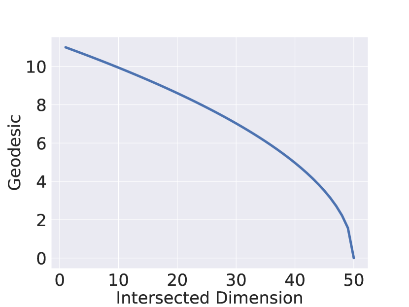
(a) Geodesic Metric

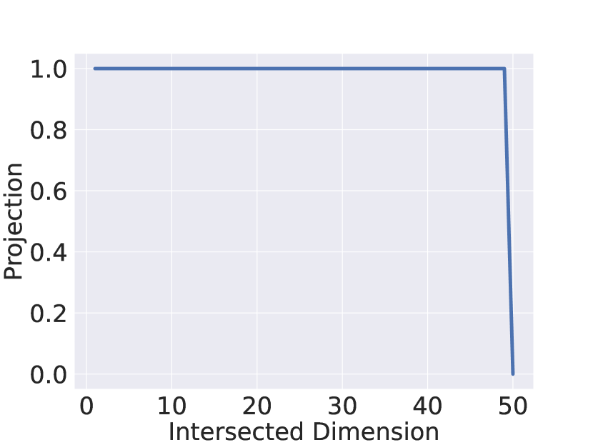
(b) Projection Metric

Figure 8: Grassmannian metric between two 50-dimensional subspaces $W,W^{\prime}\in\textrm{Gr}(50,{\mathbb{R}}^{512})$ for each intersected dimension $k_{0}=\dim\left(W\cap W^{\prime}\right)$. While the Geodesic Metric monotonically decreases as more dimensions intersect, the Projection Metric cannot discriminate $0\leq k_{0}\leq 49$.

Appendix E Robustness to preprocessing

In this section, we assessed the robustness of Distortion $\mathcal{D}_{\mathcal{M}}$ to preprocessing hyperparameter $\theta_{pre}$. Figure 9 presents the distribution of 1k samples of distortion before taking an expectation, i.e., $\left(d^{k}_{\mathrm{geo}}\left(\,T_{\mathbf{w}_{1}}\mathcal{M}^{k}_{\mathbf{w}_{1}},T_{\mathbf{w}_{2}}\mathcal{M}^{k}_{\mathbf{w}_{2}}\right)/I_{local}\right)$, for each intermediate layer. In Fig 9, increasing $\theta_{pre}$ makes an overall translation of Distortion. However, the relative ordering between the layers remains the same. The low Distortion score of layer 8 provides an explanation for the superior disentanglement of $\mathcal{W}$-space observed in many literatures (Karras et al., 2019; Härkönen et al., 2020). Moreover, the results suggest that the min-distorted layer $7$ can serve as a similar-or-better alternative.

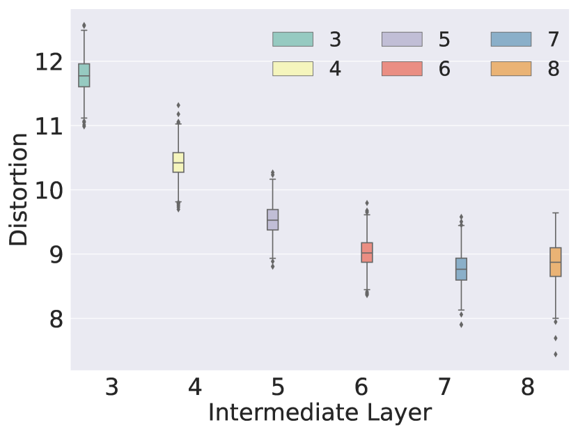
(a) $\theta_{pre}=0.0005$

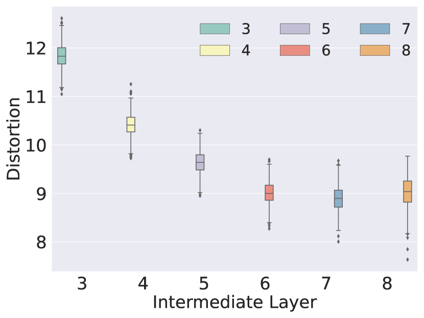
(b) $\theta_{pre}=0.001$

(c) $\theta_{pre}=0.005$

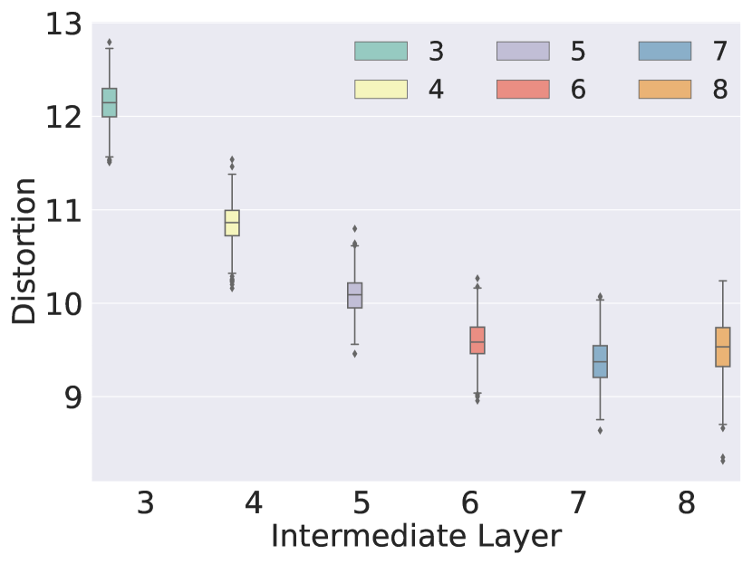
(d) $\theta_{pre}=0.01$

Figure 9: Robustness of Distortion metric $\mathcal{D}$ to $\theta_{pre}$ of StyleGAN2 on FFHQ.

Appendix F Architecture diagram of StyleGANs

Appendix G Robustness of Correlations to preprocessing

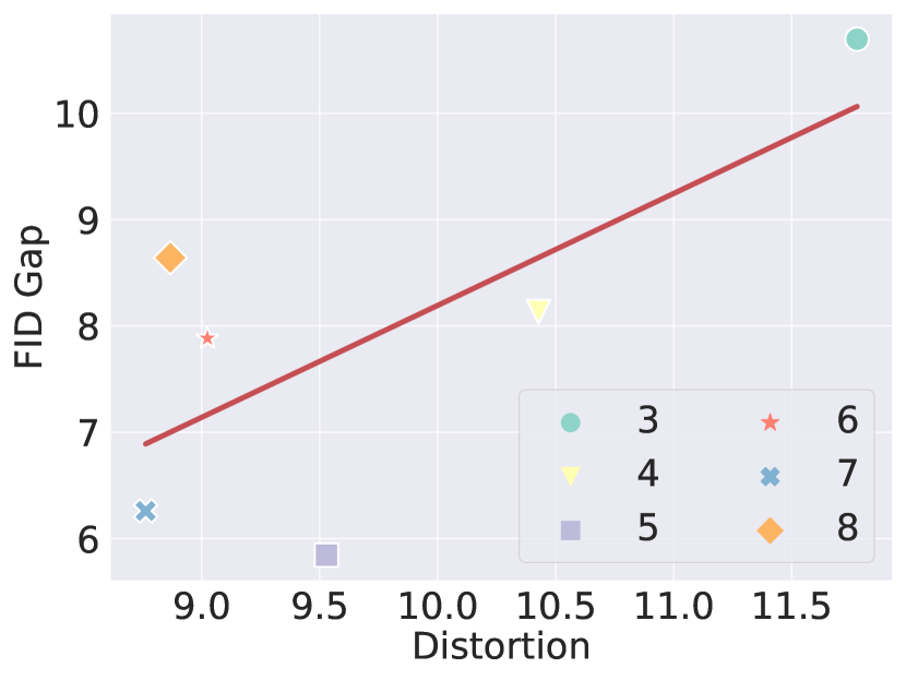
(a) $\theta_{pre}=0.0005$, $\rho=0.706$

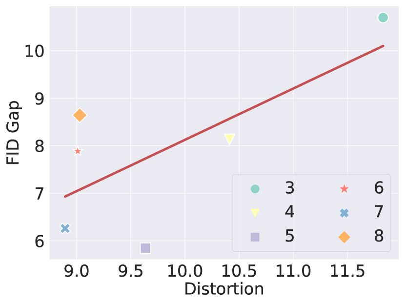
(b) $\theta_{pre}=0.001$, $\rho=0.706$

(c) $\theta_{pre}=0.005$, $\rho=0.701$

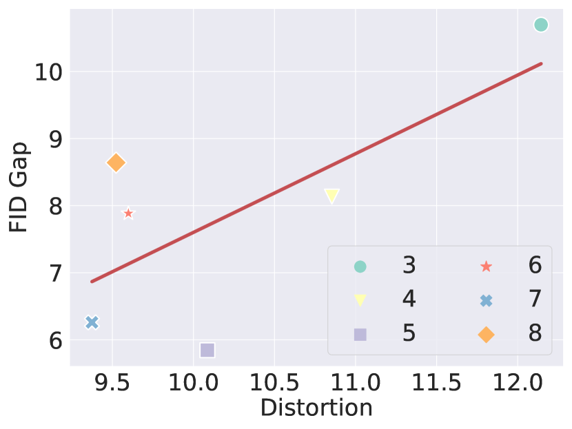
(d) $\theta_{pre}=0.01$, $\rho=0.715$

Figure 11: Correlation between Distortion metric and FID gap of StyleGAN2 on FFHQ. FID gap represents the difference between FID (Heusel et al., 2017) score of Local Basis (Choi et al., 2022b) and the global basis (Härkönen et al., 2020). Each FID score is measure for 50k samples of latent-perturbed images along the first component of Local Basis and GANSpace. The perturbation intensity is fixed to 3. Each point represents a $i$-th intermediate layer in the mapping network, and the red-line illustrates the linear regression of these points. $\rho$ denotes the Pearson correlation coefficient of Distortion and FID. The positive correlation between Distortion and FID remains robust regardless of $\theta_{pre}$.

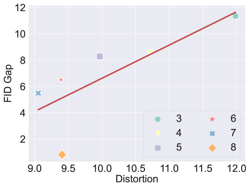
(a) $\theta_{pre}=0.0005$, $\rho=0.777$

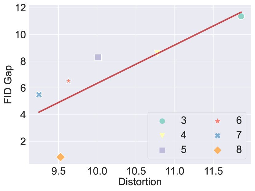
(b) $\theta_{pre}=0.001$, $\rho=0.786$

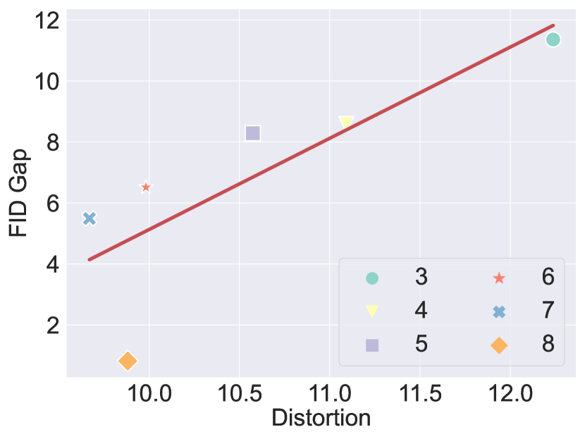
(c) $\theta_{pre}=0.005$, $\rho=0.811$

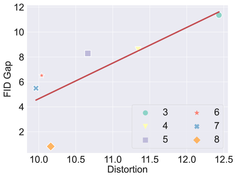
(d) $\theta_{pre}=0.01$, $\rho=0.775$

Figure 12: Correlation between Distortion metric and FID gap of StyleGAN2 with config E on FFHQ.

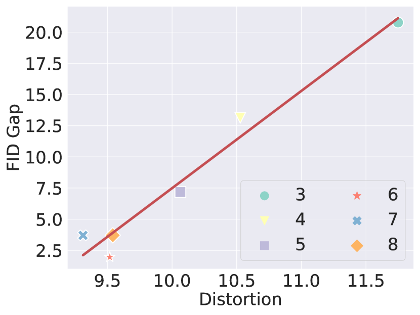
(a) $\theta_{pre}=0.0005$, $\rho=0.98$

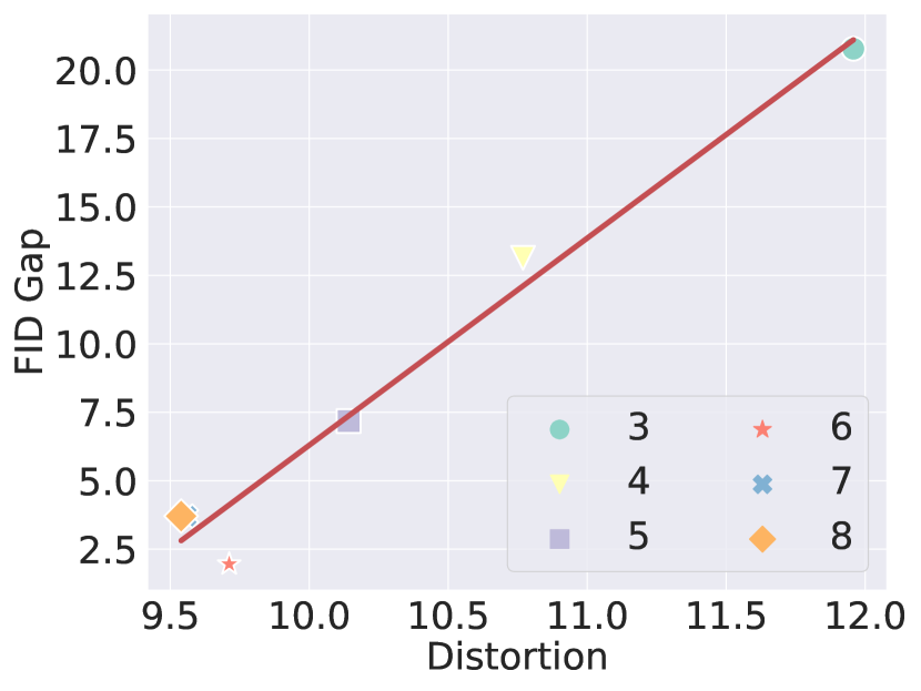
(b) $\theta_{pre}=0.001$, $\rho=0.986$

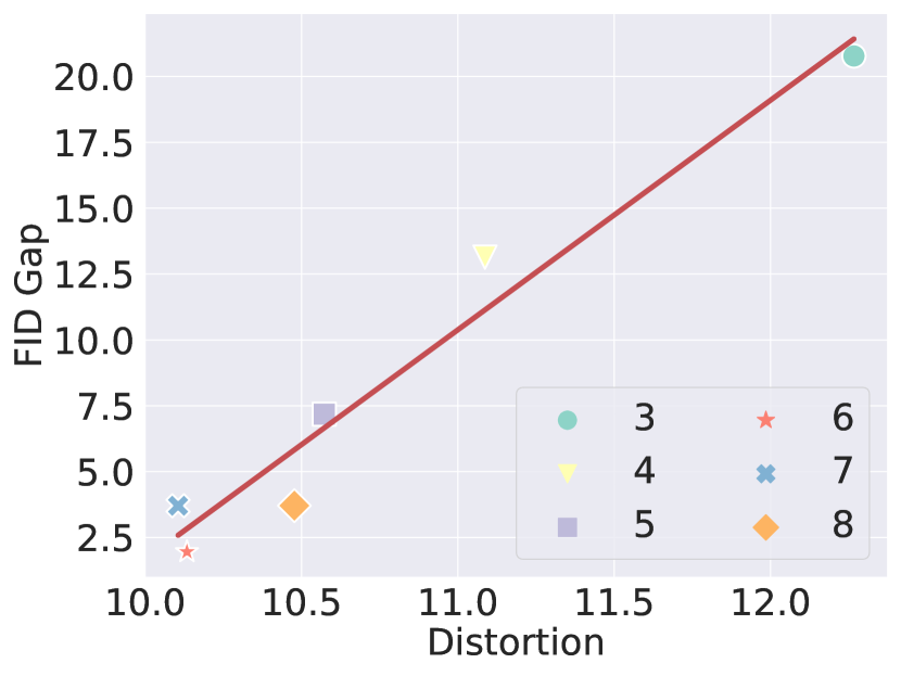
(c) $\theta_{pre}=0.005$, $\rho=0.978$

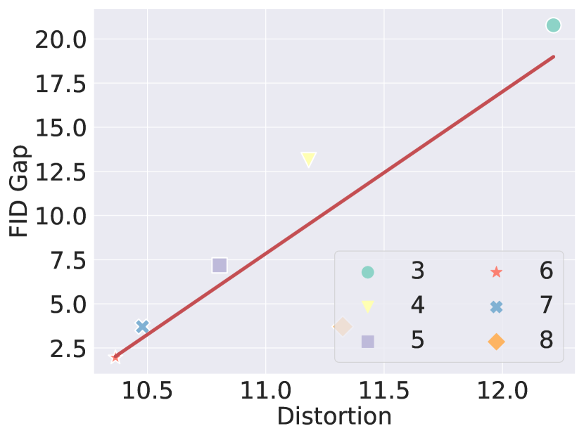
(d) $\theta_{pre}=0.01$, $\rho=0.859$

Figure 13: Correlation between Distortion metric and FID gap of StyleGAN2 on LSUN Cat (Yu et al., 2015).

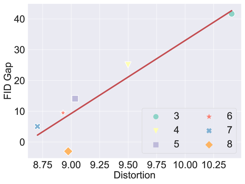
(a) $\theta_{pre}=0.00005$, $\rho=0.926$

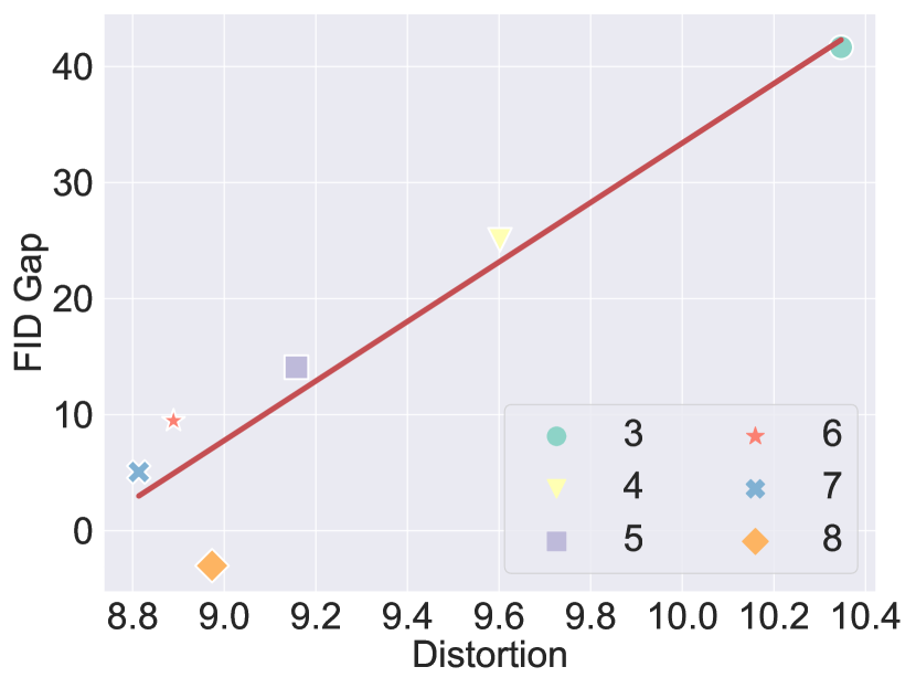
(b) $\theta_{pre}=0.0001$, $\rho=0.945$

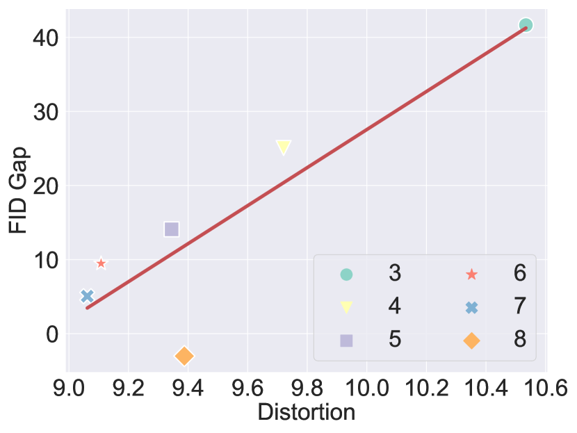
(c) $\theta_{pre}=0.0005$, $\rho=0.883$

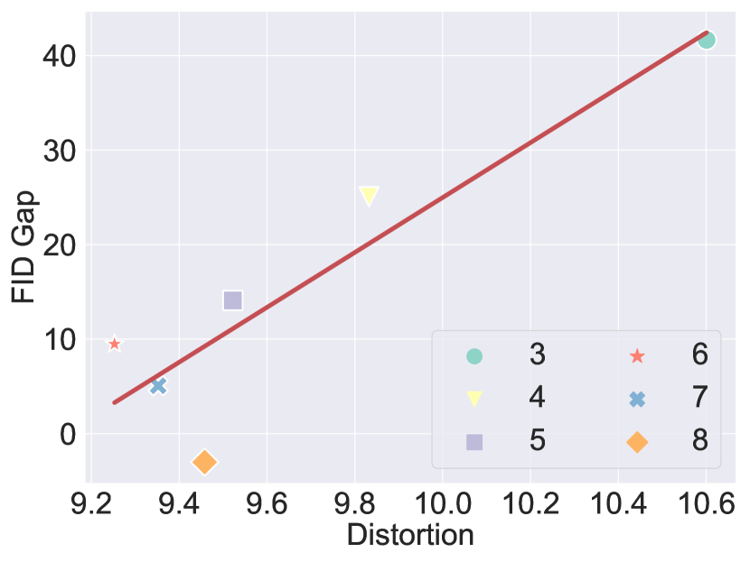
(d) $\theta_{pre}=0.001$, $\rho=0.907$

Figure 14: Correlation between Distortion metric and FID gap of StyleGAN2 on LSUN Horse.

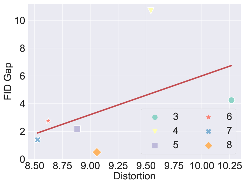
(a) $\theta_{pre}=0.00005$, $\rho=0.496$

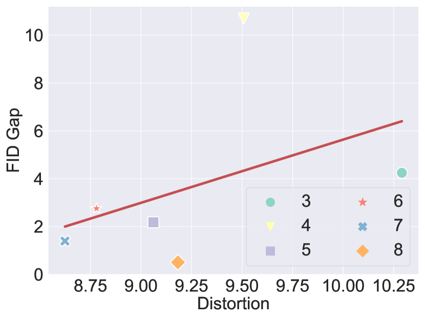
(b) $\theta_{pre}=0.0001$, $\rho=0.430$

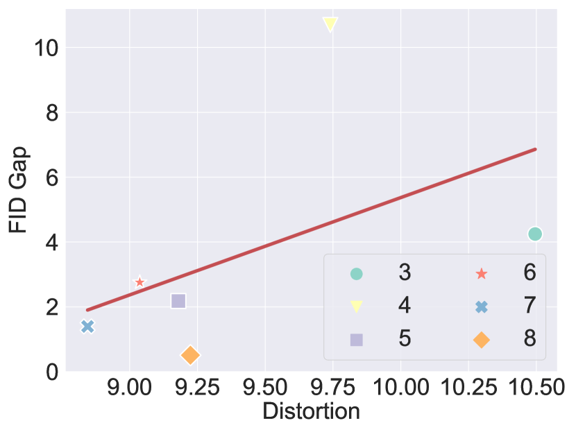
(c) $\theta_{pre}=0.0005$, $\rho=0.494$

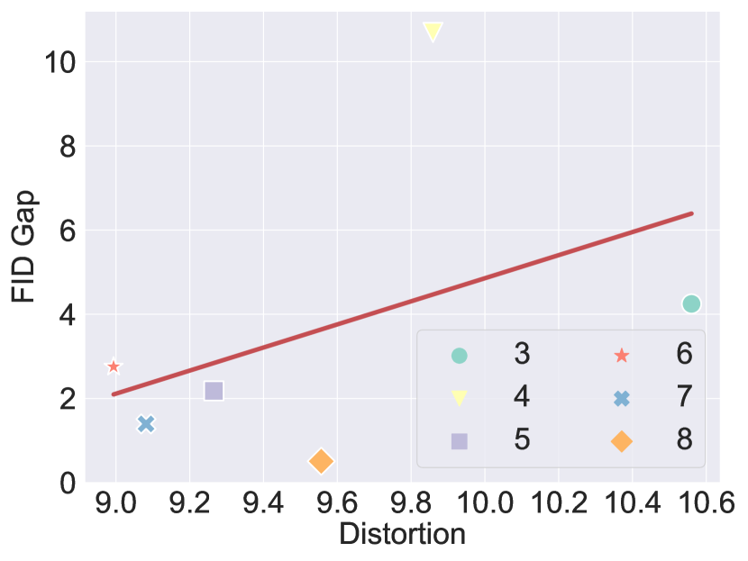
(d) $\theta_{pre}=0.001$, $\rho=0.437$

Figure 15: Correlation between Distortion metric and FID gap of StyleGAN2 on LSUN Church.

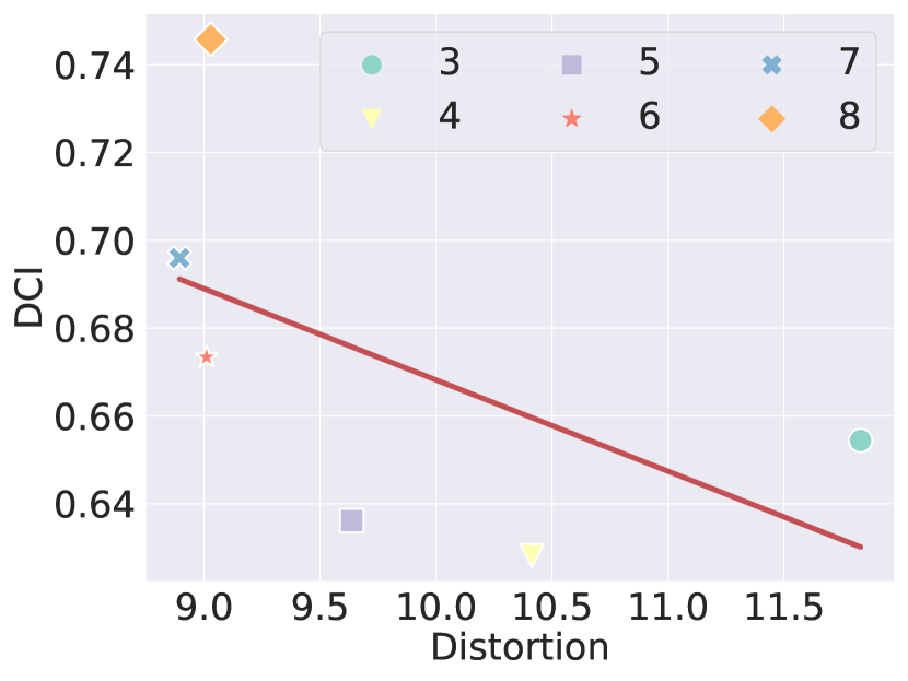
(a) $\theta_{pre}=0.001$, $\rho=-0.545$

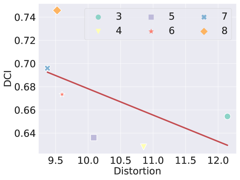
(b) $\theta_{pre}=0.01$, $\rho=-0.555$

(c) $\theta_{pre}=0.0005$, $\rho=-0.574$

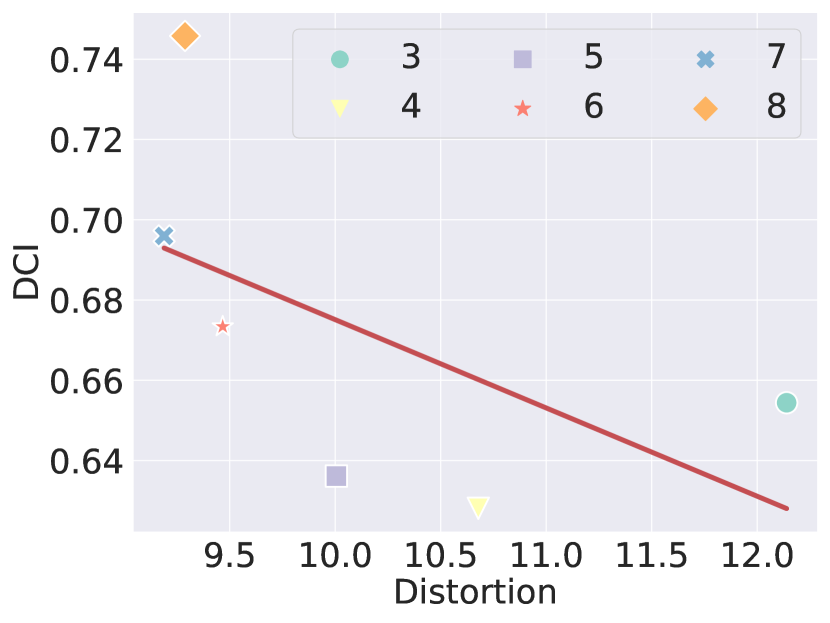
(d) $\theta_{pre}=0.005$, $\rho=-0.569$

Figure 16: Correlation between Distortion metric and DCI of StyleGAN2 on FFHQ. Each DCI (Eastwood & Williams, 2018) score is evaluated for 10k samples of generated images, while the attribute label is generated by 40 attribute classifiers pre-trained on CelebA (Liu et al., 2015). As in Fig 11, each point and red-line represents the intermediate layers and linear regression, respectively. The Distortion and DCI score show a negative correlation.

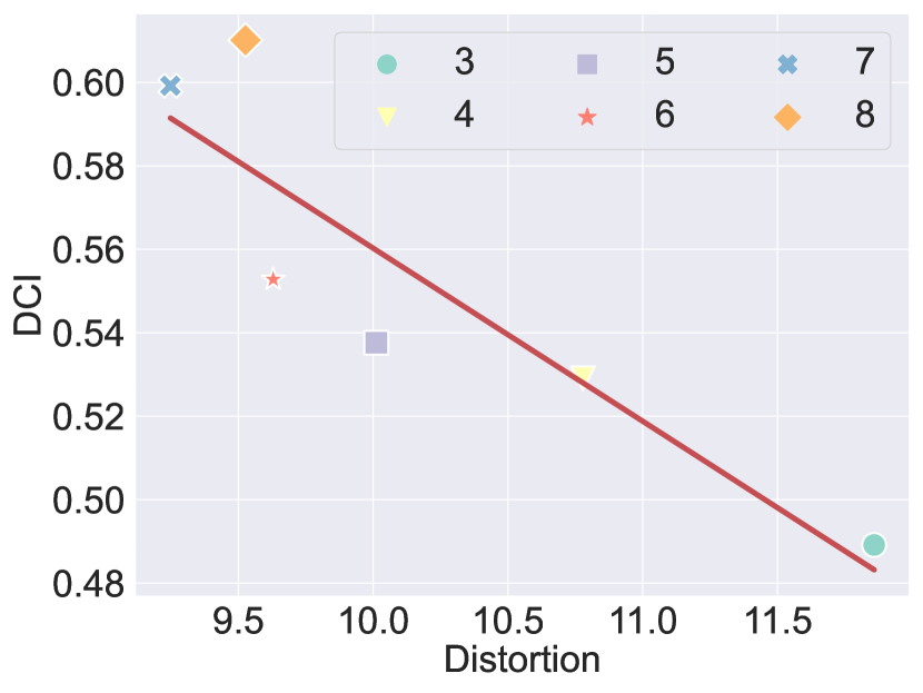
(a) $\theta_{pre}=0.001$, $\rho=-0.896$

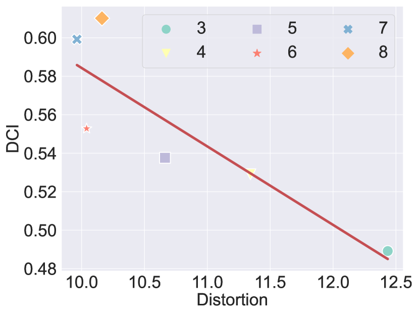
(b) $\theta_{pre}=0.01$, $\rho=-0.868$

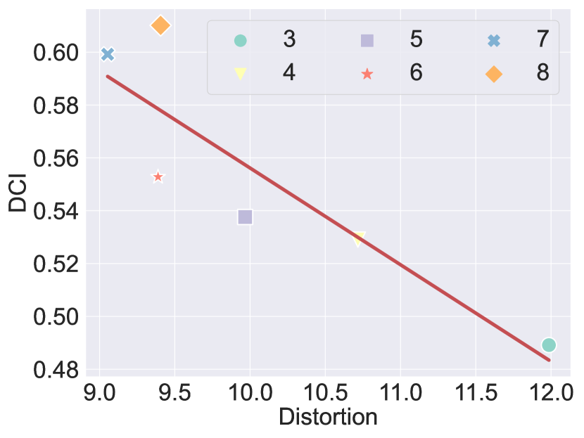
(c) $\theta_{pre}=0.0005$, $\rho=-0.887$

(d) $\theta_{pre}=0.005$, $\rho=-0.910$

Figure 17: Correlation between Distortion metric and DCI of StyleGAN2 with config E on FFHQ.

(a) $\theta_{pre}=0.001$, $\rho=-0.756$

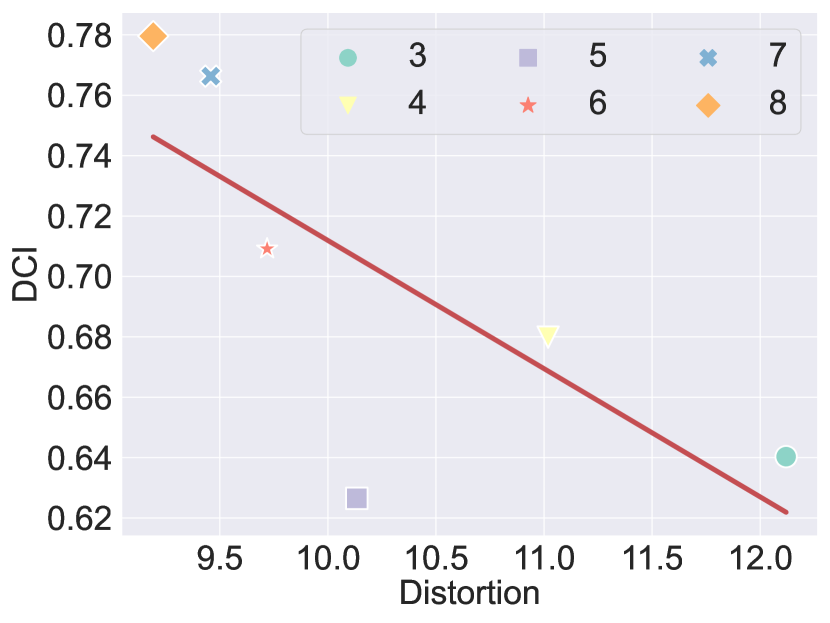
(b) $\theta_{pre}=0.01$, $\rho=-0.740$

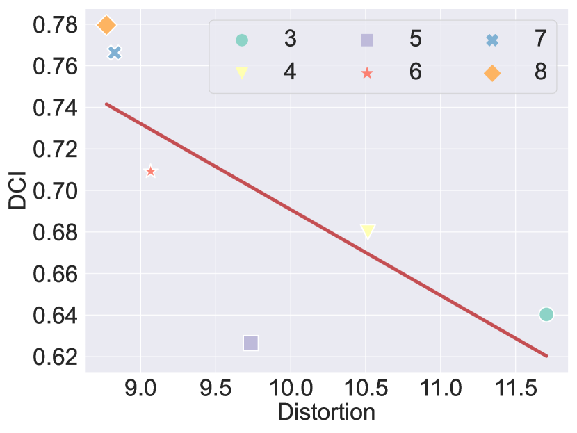
(c) $\theta_{pre}=0.0005$, $\rho=-0.752$

(d) $\theta_{pre}=0.005$, $\rho=-0.742$

Figure 18: Correlation between Distortion metric and DCI of StyleGAN1 on FFHQ.

Appendix H Additional Experimental results

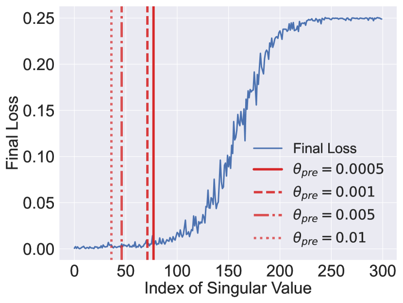
(a) $\|\mathbf{w}_{ptb}-\mathbf{w}_{init}\|=0.5$

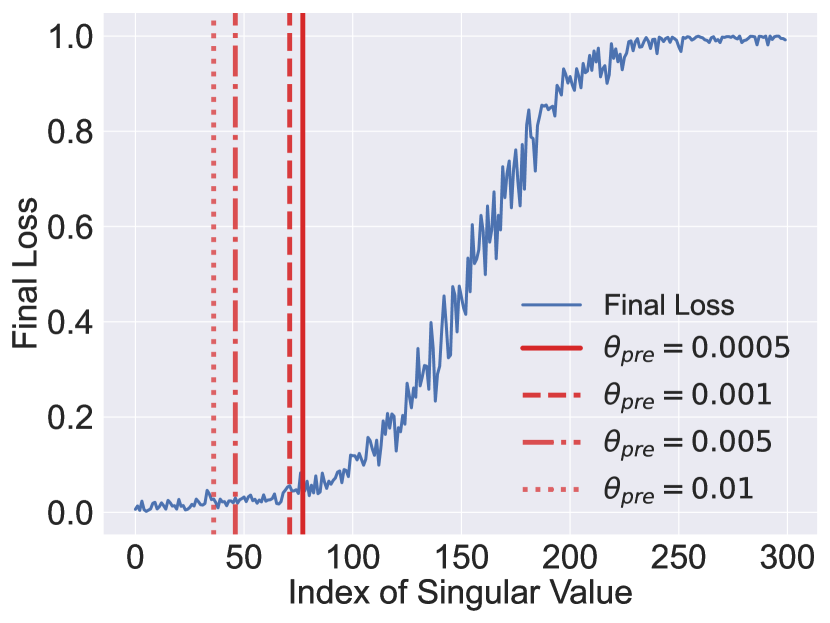
(b) $\|\mathbf{w}_{ptb}-\mathbf{w}_{init}\|=1$

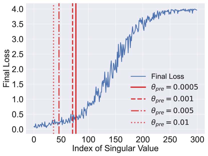
(c) $\|\mathbf{w}_{ptb}-\mathbf{w}_{init}\|=2$

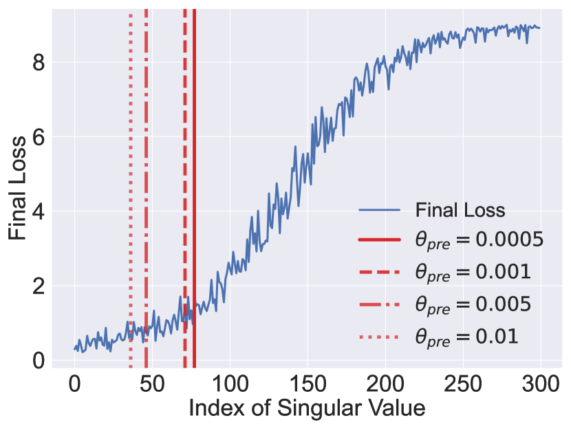
(d) $\|\mathbf{w}_{ptb}-\mathbf{w}_{init}\|=3$

Figure 19: Off-manifold Results in $\mathcal{W}$-space of StyleGAN2 on FFHQ. The red vertical lines denote the estimated local dimension for various $\theta_{pre}$. The small final loss implies that the linear perturbation along that Local Basis component stays inside the learned latent manifold. For every perturbation intensity, there is a transition point from a slow increase to a sharp increase, which is interpreted as an escape from the manifold. The results demonstrate that the proposed dimension estimation algorithm finds a reasonable point without crossing the transition point. In our case, these results are interpreted as choosing the principal part of the manifold without overestimating its dimension.

(a) $\theta_{pre}=0.0005$

(b) $\theta_{pre}=0.001$

(c) $\theta_{pre}=0.005$

(d) $\theta_{pre}=0.01$

Figure 20: Local Dimension Distribution of the intermediate layers in the mapping network of StyleGAN2 on FFHQ. Each figure presents the distribution of estimated local dimension at each intermediate layer as we vary $\theta_{pre}$. The distributions are illustrated for 1k samples, respectively. The algorithm gives a rather unstable dimension estimate on the most unsparse first layer (Fig 2(a)) due to its isotropic gaussian assumption. However, this phenomenon is not observed in the layers with moderate depth, i.e., from 3 to 8. As we introduce the higher preprocessing ratio $\theta_{pre}$, the algorithm gives more strict, i.e., smaller, dimension estimates. Nevertheless, the relative trend between layers is the same. The deeper the latent manifold, the smaller its dimension.

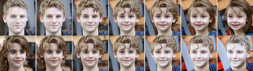
(a) Traversal along Axis 0 and 1

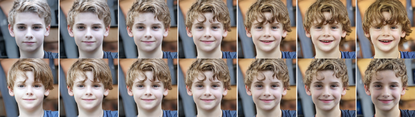
(b) Traversal along Axis 34 and 35 - $\theta_{pre}=0.01$

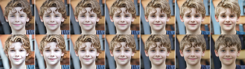
(c) Traversal along Axis 43 and 44 - $\theta_{pre}=0.005$

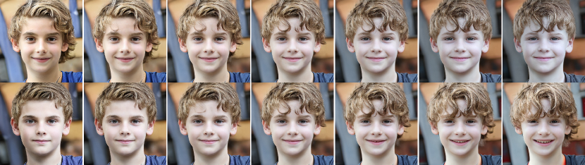
(d) Traversal along Axis 67 and 68 - $\theta_{pre}=0.001$

(e) Traversal along Axis 78 and 79 - $\theta_{pre}=0.0005$

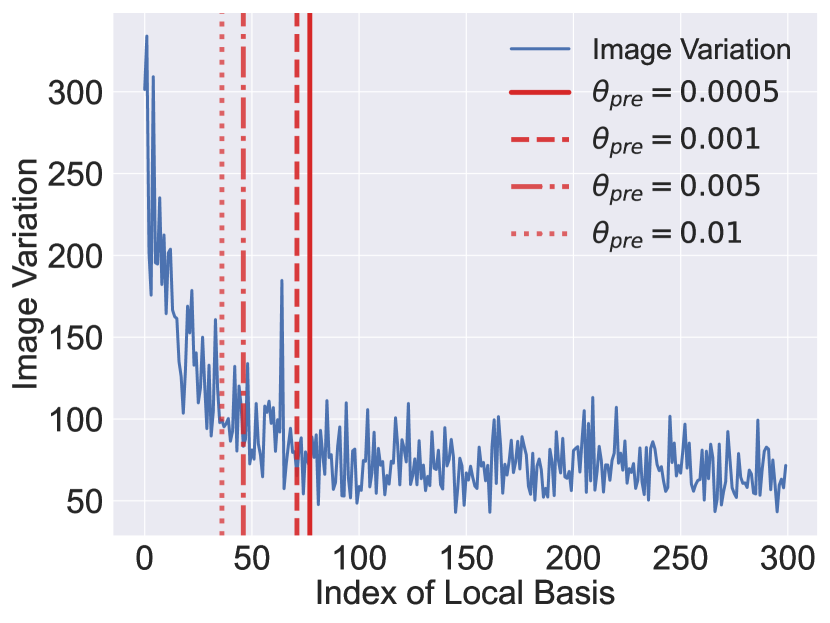
(f) Image variation intensity

Figure 21: Local Dimension Evaluation in Image Space of StyleGAN2 on FFHQ. Figure 21(b)-21(e) show image traversals along the $(d-1)$-th and $d$-th axis where $d$ denotes the estimated local dimension for each $\theta_{pre}$. Fig 21(f) presents the image variation intensity $\|\nabla_{\mathbf{v}_{i}^{\mathbf{w}}}g(\mathbf{w})\|_{F}$ along each Local Basis $\mathbf{v}_{i}$. $\|\nabla_{\mathbf{v}_{i}^{\mathbf{w}}}g(\mathbf{w})\|_{F}$ is evaluated by the finite difference with stepsize=0.01. Note that while Local Basis is discovered by analyzing only the subnetwork from the input to target latent space, the corresponding image variation monotonically decreases and saturates. Moreover, the estimated local dimension includes the major variations in the image space. This can be observed in the image traversals. The image traversals around the estimated dimension (Fig 21(b)-21(e)) show much smaller image variations compared to Axis 0 and 1 (Fig 21(a)).

Appendix I Comparison of Semantic Disentanglement

Using our Distortion metric, we chose the Max-distorted layer 3 and Min-distorted layer 7 from the mapping network of StyleGAN2-FFHQ (Karras et al., 2020b). These two layers are compared with the renowned $\mathcal{W}$-space (layer 8). Each image traversal is obtained by perturbing a latent variable along the global basis from GANSpace (Härkönen et al., 2020).

(a) Max-distorted layer 3

(b) Min-distorted layer 7

(c) Layer 8 ($\mathcal{W}$-space)

Figure 23: Comparison of Semantic Disentanglement between Layers 3, 7, 8 for the semantic ”Open Mouth”. Layer 7 exhibits a disentangled semantic variation of ”Open mouth” without changing the face, such as a longer nose in Layer 8. Layer 3 shows only minor facial expression changes.

(a) Max-distorted layer 3

(b) Min-distorted layer 7

(c) Layer 8 ($\mathcal{W}$-space)

Figure 24: Comparison of Semantic Disentanglement between Layers 3, 7, 8 for the semantic ”Face Bright”. Layer 8 shows an entangled semantic variation of ”Lipstick” and ”Face Bright” on the right end. On Layer 3, the traversal toward the right end does not show ”Face Dark” semantics.

(a) Max-distorted layer 3

(b) Min-distorted layer 7

(c) Layer 8 ($\mathcal{W}$-space)

Figure 25: Comparison of Semantic Disentanglement between Layers 3, 7, 8 for the semantic ”Gender”. On Layer 3, the image traversal shows an entangled semantic variation of ”Gender” and ”Big face” on the right end. Also, Layer 8 exhibits an entangled semantic variation of ”Gender” and ”Age”.

(a) Max-distorted layer 3

(b) Min-distorted layer 7

(c) Layer 8 ($\mathcal{W}$-space)

Figure 26: Comparison of Semantic Disentanglement between Layers 3, 7, 8 for the semantic ”Light Up”. Layer 8 exhibits an entangled semantic variation of ”Light Down” and ”Brown hair” on the right end. On the left end of Layer 3, the traversal shows the ”Bright right” transformation. However, the traversal at the right end of Layer 3 does not present the ”Bright left” transformation, while showing no shadow on the face. But, the traversal on Layer 7 shows a natural brightness change on the entire face.

Appendix J Additional Subspace Traversal Comparisons

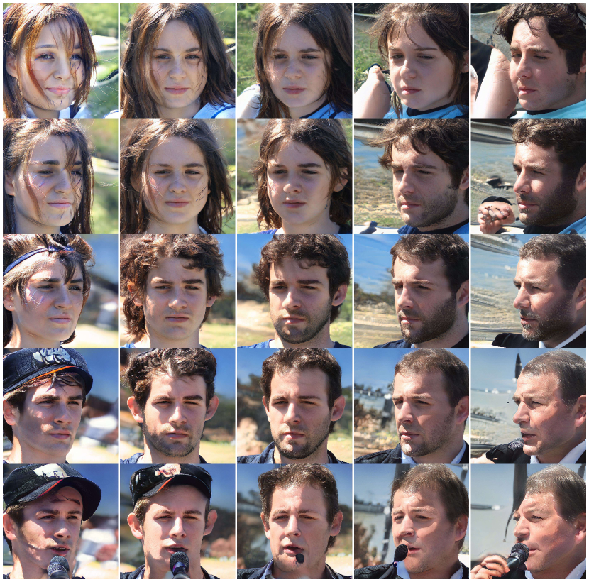
(a) Min-distorted layer - Global Basis

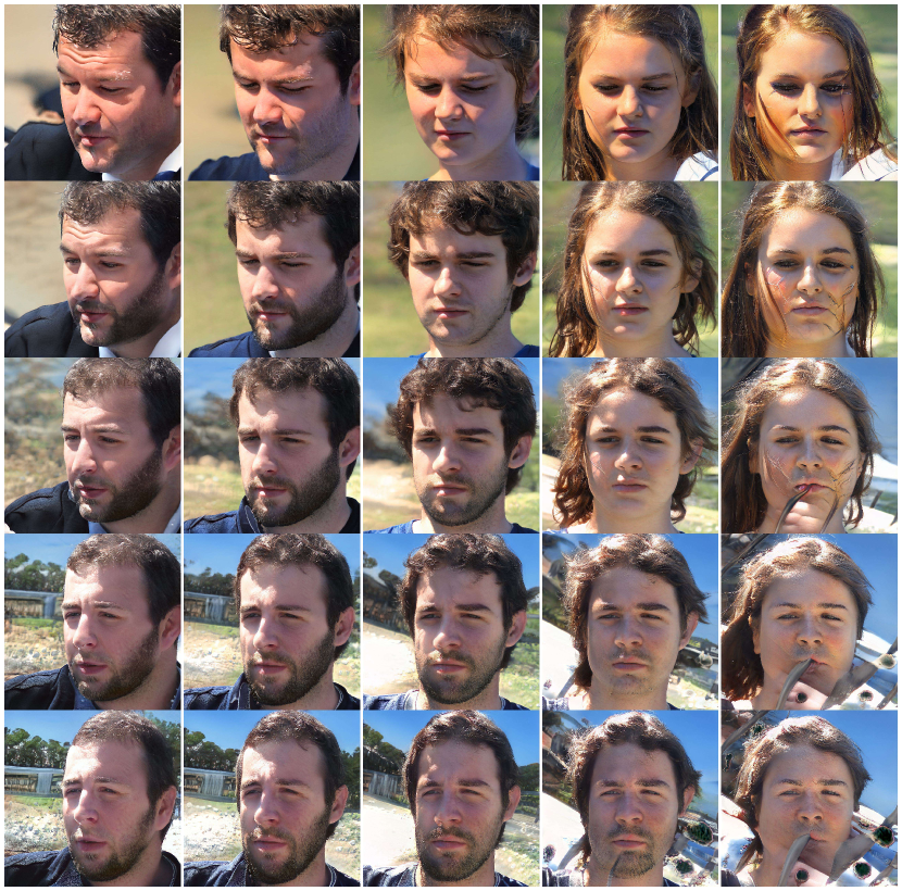
(b) Min-distorted layer - Local Basis

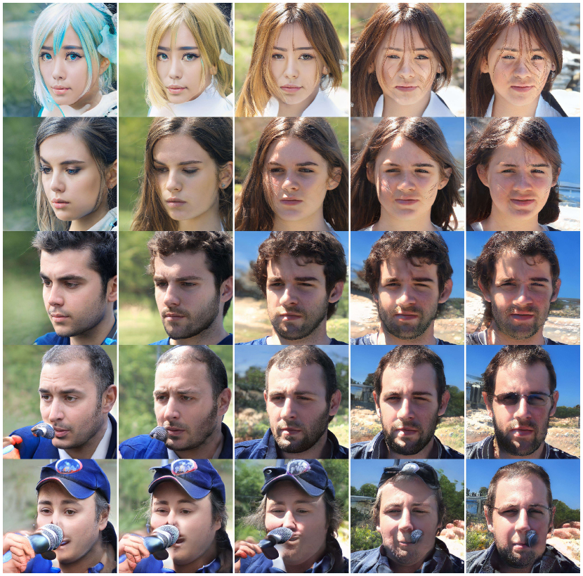
(c) Max-distorted layer - Global Basis

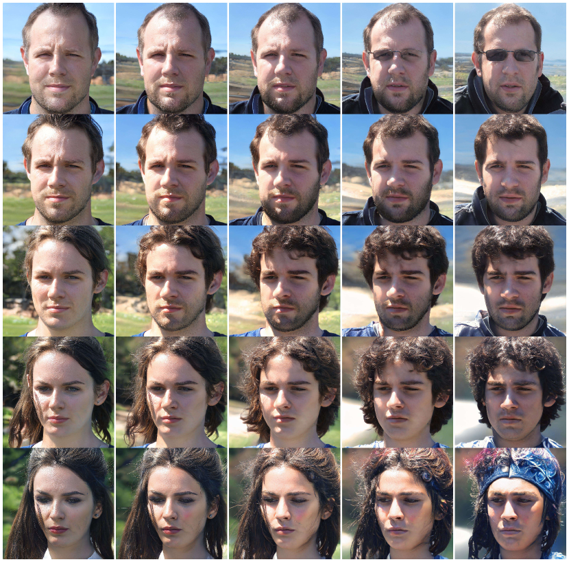
(d) Max-distorted layer - Local Basis

Figure 27: Subspace Traversal (Choi et al., 2022b) on the min-distorted ($7$th) and max-distorted ($3$rd) intermediate layers along the global basis (Härkönen et al., 2020) and Local Basis (Choi et al., 2022b) of StyleGAN2 on FFHQ. The initial image (center) is traversed along the $1$st (horizontal) and $2$nd (vertical) components of the chosen traversal directions with the perturbation intensity 9. The global basis shows a decent image quality on the min-distorted layer, similar to Local Basis. However, on the max-distorted layer, the subspace traversal along global basis exhibits significant failures at corners, such as image collapse (lower-left), visual artifacts (lower-right), and unnatural transformations (top-left).

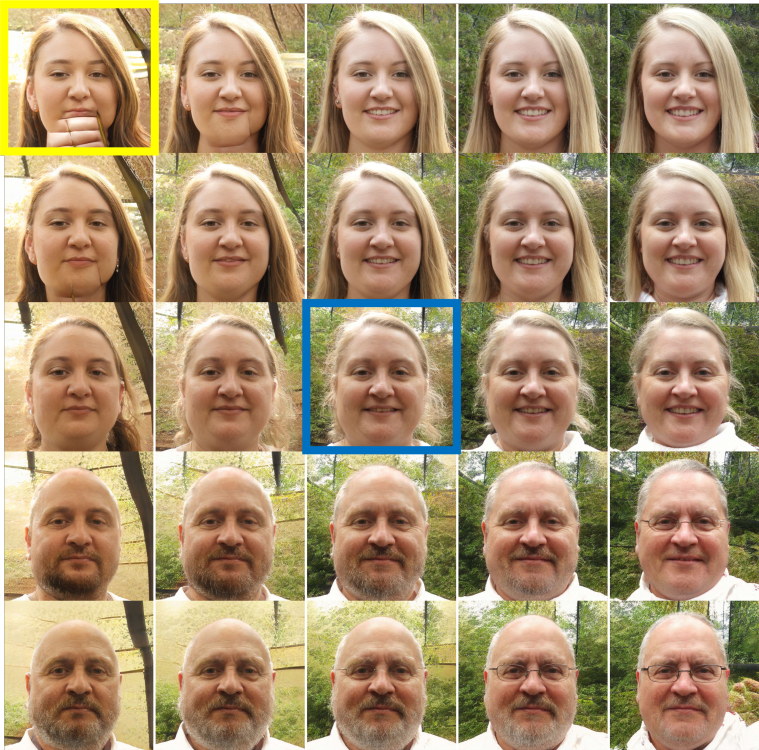
(a) Max-distorted layer 3

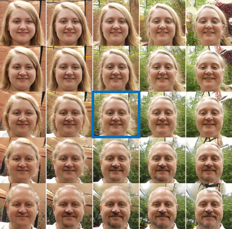
(b) Min-distorted layer 7

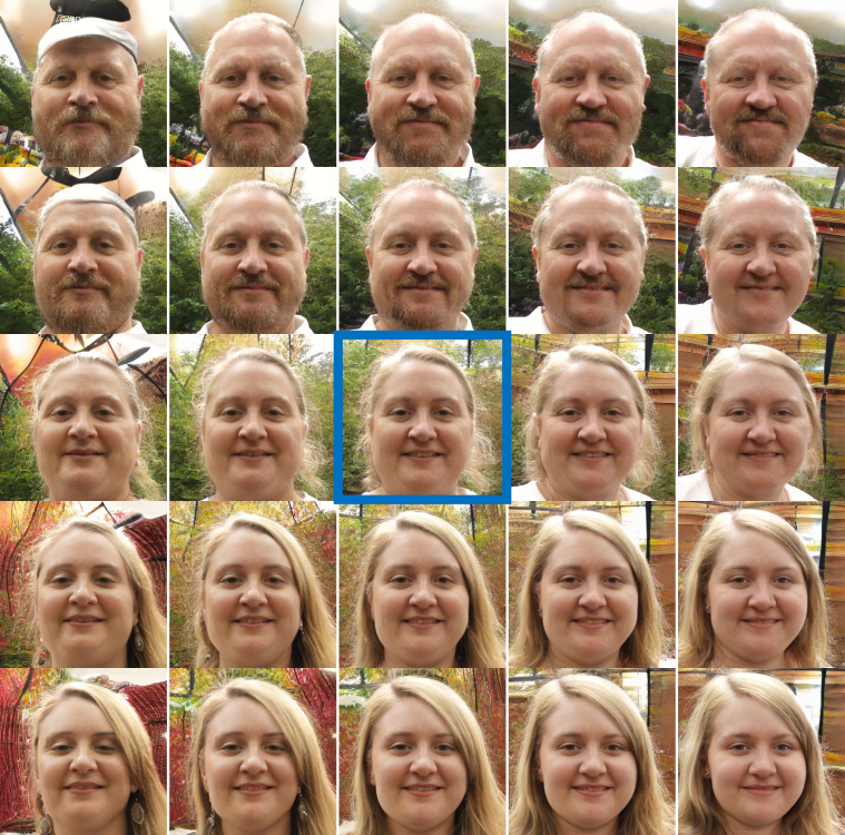
(c) Layer 8 ($\mathcal{W}$-space)

Figure 28: Subspace Traversal on StyleGAN2-FFHQ. The upper-left corner of layer 3 is severely deteriorated.

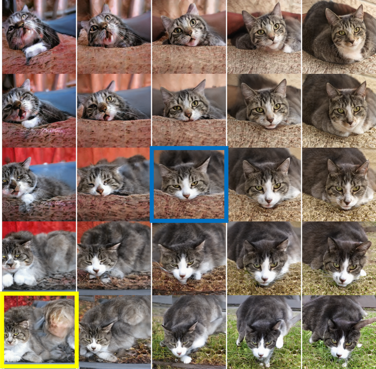
(a) Max-distorted layer 3

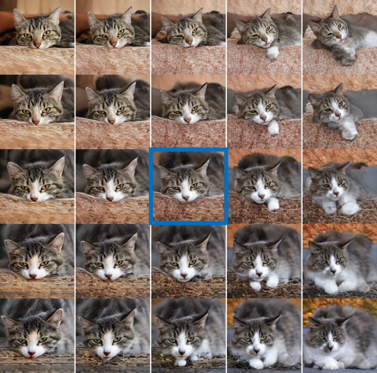
(b) Min-distorted layer 6

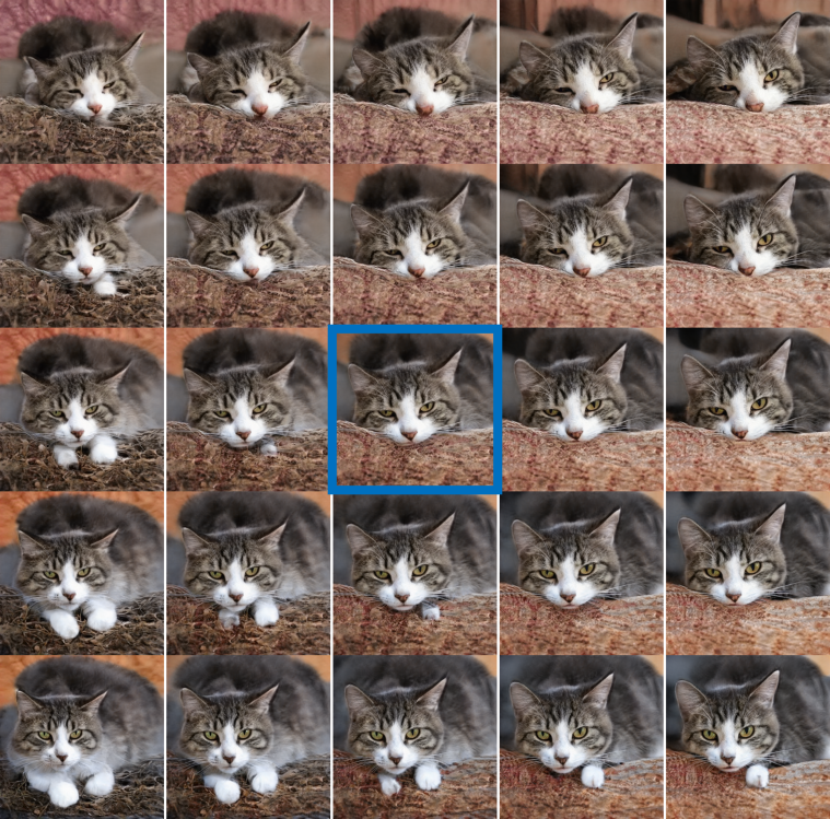
(c) Layer 8 ($\mathcal{W}$-space)

Figure 29: Subspace Traversal on StyleGAN2-LSUN Cat. The lower-left corner of layer 3 are severely deteriorated.

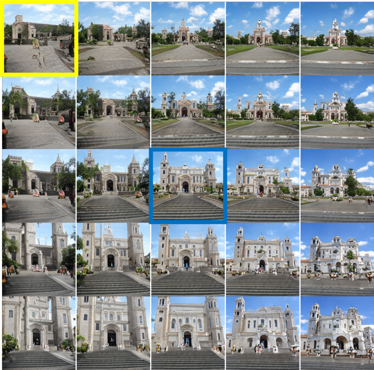
(a) Max-distorted layer 3

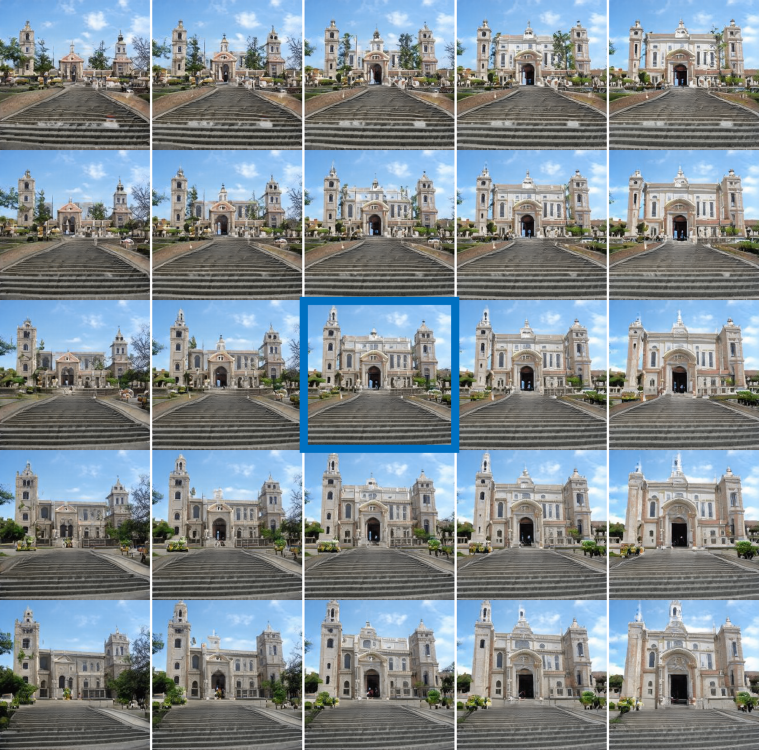
(b) Min-distorted layer 6

(c) Layer 8 ($\mathcal{W}$-space)

Figure 30: Subspace Traversal on StyleGAN2-LSUN Church. The upper-left corner of layer 3 are severely deteriorated.

(a) Max-distorted layer 3

(b) Min-distorted layer 6

(c) Layer 8 ($\mathcal{W}$-space)

Figure 31: Subspace Traversal on StyleGAN2-LSUN Horse. The right sides of layer 3 are severely deteriorated.

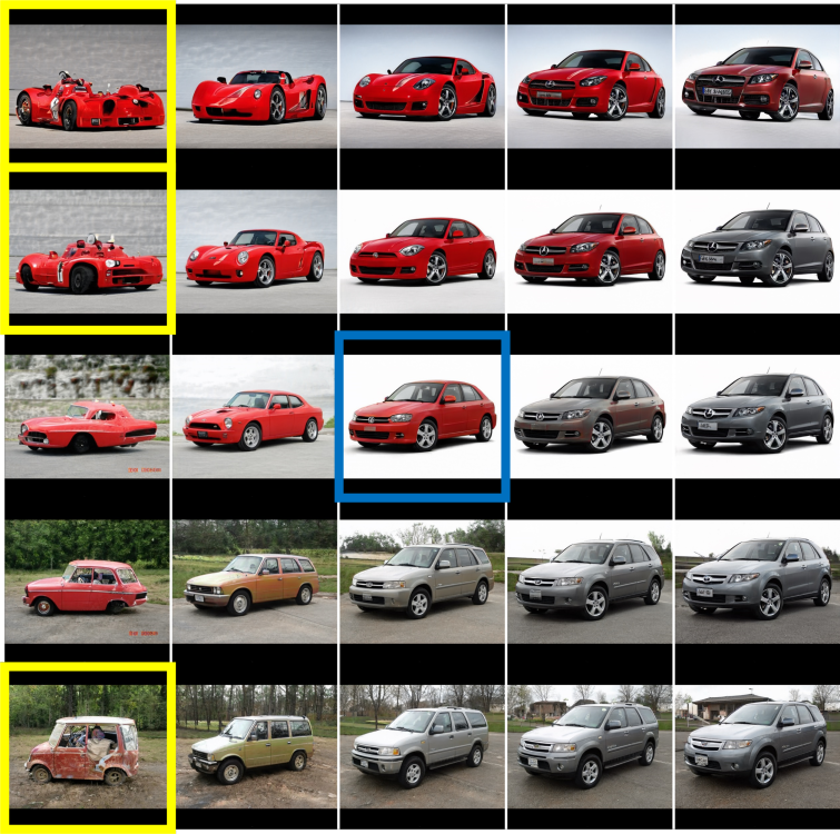
(a) Max-distorted layer 3

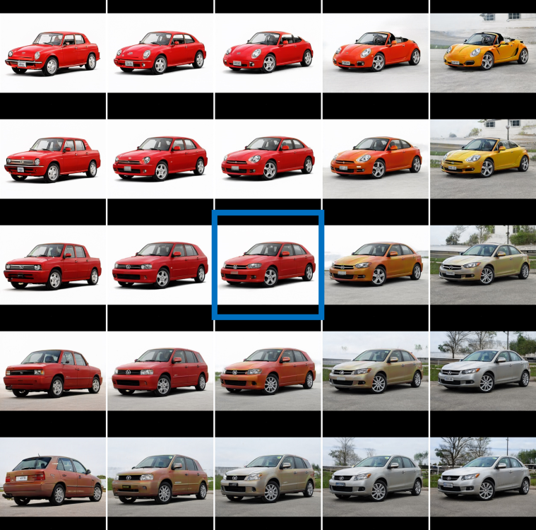
(b) Min-distorted layer 7

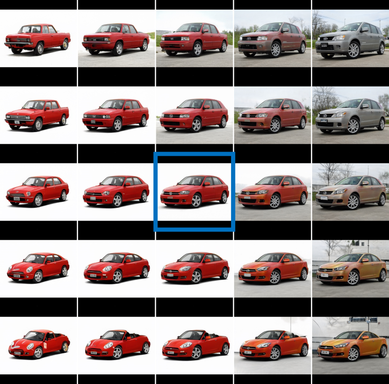
(c) Layer 8 ($\mathcal{W}$-space)

Figure 32: Linear Traversal on StyleGAN2-LSUN Cars. The left sides of layer 3 are severely deteriorated.

References

- Abdal et al. (2019) Abdal, R., Qin, Y., and Wonka, P. Image2stylegan: How to embed images into the stylegan latent space? In Proceedings of the IEEE/CVF International Conference on Computer Vision, pp. 4432–4441, 2019.
- Abdal et al. (2021) Abdal, R., Zhu, P., Mitra, N. J., and Wonka, P. Styleflow: Attribute-conditioned exploration of stylegan-generated images using conditional continuous normalizing flows. ACM Transactions on Graphics (TOG), 40(3):1–21, 2021.
- Bengio et al. (2013) Bengio, Y., Courville, A., and Vincent, P. Representation learning: A review and new perspectives. IEEE transactions on pattern analysis and machine intelligence, 35(8):1798–1828, 2013.
- Boothby (1986) Boothby, W. M. An introduction to differentiable manifolds and Riemannian geometry. Academic press, 1986.
- Boyd et al. (2011) Boyd, S., Parikh, N., Chu, E., Peleato, B., Eckstein, J., et al. Distributed optimization and statistical learning via the alternating direction method of multipliers. Foundations and Trends® in Machine learning, 3(1):1–122, 2011.
- Brock et al. (2018) Brock, A., Donahue, J., and Simonyan, K. Large scale gan training for high fidelity natural image synthesis. In International Conference on Learning Representations, 2018.
- Candès et al. (2011) Candès, E. J., Li, X., Ma, Y., and Wright, J. Robust principal component analysis? Journal of the ACM (JACM), 58(3), 2011. ISSN 0004-5411. doi: 10.1145/1970392.1970395.
- Choi et al. (2022a) Choi, J., Hwang, G., Cho, H., and Kang, M. Finding the global semantic representation in gan through frechet mean. arXiv preprint arXiv:2210.05509, 2022a.
- Choi et al. (2022b) Choi, J., Lee, J., Yoon, C., Park, J. H., Hwang, G., and Kang, M. Do not escape from the manifold: Discovering the local coordinates on the latent space of GANs. In International Conference on Learning Representations, 2022b.
- Donoho & Gavish (2014) Donoho, D. and Gavish, M. Minimax risk of matrix denoising by singular value thresholding. The Annals of Statistics, 42(6):2413–2440, 2014.
- Eastwood & Williams (2018) Eastwood, C. and Williams, C. K. A framework for the quantitative evaluation of disentangled representations. In International Conference on Learning Representations, 2018.
- Eckart & Young (1936) Eckart, C. and Young, G. The approximation of one matrix by another of lower rank. Psychometrika, 1(3):211–218, 1936.
- Goetschalckx et al. (2019) Goetschalckx, L., Andonian, A., Oliva, A., and Isola, P. Ganalyze: Toward visual definitions of cognitive image properties. In Proceedings of the IEEE/CVF International Conference on Computer Vision, pp. 5744–5753, 2019.
- Goodfellow et al. (2014) Goodfellow, I. J., Pouget-Abadie, J., Mirza, M., Xu, B., Warde-Farley, D., Ozair, S., Courville, A. C., and Bengio, Y. Generative adversarial nets. In NIPS, 2014.
- Härkönen et al. (2020) Härkönen, E., Hertzmann, A., Lehtinen, J., and Paris, S. Ganspace: Discovering interpretable gan controls. Advances in Neural Information Processing Systems, 33, 2020.
- Heusel et al. (2017) Heusel, M., Ramsauer, H., Unterthiner, T., Nessler, B., and Hochreiter, S. Gans trained by a two time-scale update rule converge to a local nash equilibrium. Advances in neural information processing systems, 30, 2017.
- Jahanian et al. (2019) Jahanian, A., Chai, L., and Isola, P. On the” steerability” of generative adversarial networks. In International Conference on Learning Representations, 2019.
- Johnstone (2001) Johnstone, I. M. On the distribution of the largest eigenvalue in principal components analysis. The Annals of statistics, 29(2):295–327, 2001.
- Karras et al. (2018) Karras, T., Aila, T., Laine, S., and Lehtinen, J. Progressive growing of gans for improved quality, stability, and variation. In International Conference on Learning Representations, 2018.
- Karras et al. (2019) Karras, T., Laine, S., and Aila, T. A style-based generator architecture for generative adversarial networks. In Proceedings of the IEEE/CVF Conference on Computer Vision and Pattern Recognition, pp. 4401–4410, 2019.
- Karras et al. (2020a) Karras, T., Aittala, M., Hellsten, J., Laine, S., Lehtinen, J., and Aila, T. Training generative adversarial networks with limited data. arXiv preprint arXiv:2006.06676, 2020a.
- Karras et al. (2020b) Karras, T., Laine, S., Aittala, M., Hellsten, J., Lehtinen, J., and Aila, T. Analyzing and improving the image quality of stylegan. In Proceedings of the IEEE/CVF Conference on Computer Vision and Pattern Recognition, pp. 8110–8119, 2020b.
- Karras et al. (2021) Karras, T., Aittala, M., Laine, S., Härkönen, E., Hellsten, J., Lehtinen, J., and Aila, T. Alias-free generative adversarial networks. Advances in Neural Information Processing Systems, 34, 2021.
- Karrasch (2017) Karrasch, D. An introduction to grassmann manifolds and their matrix representation. 2017.
- Kingma & Ba (2015) Kingma, D. P. and Ba, J. Adam: A method for stochastic optimization. In International Conference on Learning Representations (ICLR), 2015.
- Kritchman & Nadler (2008) Kritchman, S. and Nadler, B. Determining the number of components in a factor model from limited noisy data. Chemometrics and Intelligent Laboratory Systems, 94(1):19–32, 2008.
- Lin et al. (2010) Lin, Z., Chen, M., and Ma, Y. The augmented lagrange multiplier method for exact recovery of corrupted low-rank matrices. arXiv preprint arXiv:1009.5055, 2010.
- Liu et al. (2015) Liu, Z., Luo, P., Wang, X., and Tang, X. Deep learning face attributes in the wild. In Proceedings of International Conference on Computer Vision (ICCV), December 2015.
- Locatello et al. (2019) Locatello, F., Bauer, S., Lucic, M., Raetsch, G., Gelly, S., Schölkopf, B., and Bachem, O. Challenging common assumptions in the unsupervised learning of disentangled representations. In International Conference on Machine Learning, pp. 4114–4124, 2019.
- Patashnik et al. (2021) Patashnik, O., Wu, Z., Shechtman, E., Cohen-Or, D., and Lischinski, D. Styleclip: Text-driven manipulation of stylegan imagery. arXiv preprint arXiv:2103.17249, 2021.
- Plumerault et al. (2020) Plumerault, A., Borgne, H. L., and Hudelot, C. Controlling generative models with continuous factors of variations. In International Conference on Learning Representations, 2020.
- Radford et al. (2016) Radford, A., Metz, L., and Chintala, S. Unsupervised representation learning with deep convolutional generative adversarial networks. In Proceedings of the International Conference on Learning Representations (ICLR), 2016.
- Ramesh et al. (2018) Ramesh, A., Choi, Y., and LeCun, Y. A spectral regularizer for unsupervised disentanglement. arXiv preprint arXiv:1812.01161, 2018.
- Sauer et al. (2022) Sauer, A., Schwarz, K., and Geiger, A. Stylegan-xl: Scaling stylegan to large diverse datasets. In Special Interest Group on Computer Graphics and Interactive Techniques Conference Proceedings, pp. 1–10, 2022.
- Shen & Zhou (2021) Shen, Y. and Zhou, B. Closed-form factorization of latent semantics in gans. In CVPR, 2021.
- Shen et al. (2020) Shen, Y., Gu, J., Tang, X., and Zhou, B. Interpreting the latent space of gans for semantic face editing. In Proceedings of the IEEE/CVF Conference on Computer Vision and Pattern Recognition, pp. 9243–9252, 2020.
- Voynov & Babenko (2020) Voynov, A. and Babenko, A. Unsupervised discovery of interpretable directions in the gan latent space. In International Conference on Machine Learning, pp. 9786–9796. PMLR, 2020.
- Wu et al. (2020) Wu, Z., Lischinski, D., and Shechtman, E. Stylespace analysis: Disentangled controls for stylegan image generation. arXiv preprint arXiv:2011.12799, 2020.
- Ye & Lim (2016) Ye, K. and Lim, L.-H. Schubert varieties and distances between subspaces of different dimensions. SIAM Journal on Matrix Analysis and Applications, 37(3):1176–1197, 2016.
- Yu et al. (2015) Yu, F., Zhang, Y., Song, S., Seff, A., and Xiao, J. Lsun: Construction of a large-scale image dataset using deep learning with humans in the loop. arXiv preprint arXiv:1506.03365, 2015.
- Zhu et al. (2021) Zhu, J., Feng, R., Shen, Y., Zhao, D., Zha, Z., Zhou, J., and Chen, Q. Low-rank subspaces in gans. arXiv preprint arXiv:2106.04488, 2021.
- Zhu et al. (2020) Zhu, P., Abdal, R., Qin, Y., Femiani, J., and Wonka, P. Improved stylegan embedding: Where are the good latents? arXiv preprint arXiv:2012.09036, 2020.