Theory of giant diode effect in $d$-wave superconductor junctions on the surface of topological insulator

Abstract

Nonreciprocal responses of noncentrosymmetric quantum materials attract recent intensive interests, which is essential for the rectification function in diodes. A recent breakthrough is the discovery of superconducting diode effect. The principle to enlarge rectification effect is highly desired to guide the design of superconducting diode. Here, we study theoretically the Josephson junction S/FI/S (S: $d$-wave superconductor, FI: ferromagnetic insulator) on the surface of a topological insulator (TI). The simultaneous existence of $\sin\varphi$, $\cos\varphi$ and $\sin 2\varphi$ terms with almost the same order in Josephson current $I(\varphi)$ is essential to get larger values of $Q$ factor given by $Q=(I_{c}^{+}-\mid I_{c}^{-}\mid)/(I_{c}^{+}+\mid I_{c}^{-}\mid)$ with $I_{c}^{+}={\rm max}(I(\varphi))$ and the negative one $I_{c}^{-}$ for macroscopic phase difference $\varphi$ of two superconductors on TI. We find that it can show a very large diode effect by tuning the crystal axes of $d$-wave superconductors and the magnetization of FI. The difference of the maximum Josephson currents $I_{c}$’s between the positive and negative directions can be about factor 2, where the current-phase relation is modified largely from the conventional one. The relevance of the zero energy Andreev bound states as Majorana bound states at the interface is also revealed. This result can pave a way to realize an efficient superconducting diode with low energy cost.

I Introduction

Nonreciprocal responses become hot topics in condensed matter physics now  Tokura and Nagaosa (2018). It is generally expected that the response to the external field is different from that of the field in the opposite direction in the presence of broken inversion symmetry $\cal{P}$. When the flow of electrons, i.e., current, is concerned, the reversal of the arrow of time, i.e., the time-reversal symmetry $\cal{T}$ is also relevant, and it often happens that the nonreciprocal transport occurs when both $\cal{P}$ and $\cal{T}$ are broken simultaneously although only $\cal{P}$ breaking is enough in some cases. In the normal state of the conductor, the typical energy scale is the Fermi energy of the order of $eV$, which is large compared with the spin-orbit interaction and Zeeman energy due to the external magnetic field, both of which are needed to introduce the asymmetry of the energy band dispersion $\varepsilon_{n}(k)$ between $k$ and $-k$. Therefore, the value of $\gamma$, which characterizes the strength of the nonreciprocal resistivity in the empirical expression

$$\rho(I)=\rho_{0}(1+\gamma IB),$$ (I.1)

is usually very small typically of the order of $\sim 10^{-3}-10^{-1}$A^-1 T^-1 Rikken et al. (2001); Krstić et al. (2002); Pop et al. (2014); Rikken and Wyder (2005). Here $\rho_{0}$ is the linear resistivity without a magnetic field, $I$ is current, and $B$ is the magnetic field. This phenomenon is called magneto-chiral anisotropy (MCA). It has been reported that $\gamma$ reaches the order of 1A^-1 T^-1 in BiTeBr, which shows a gigantic bulk Rashba splitting Ideue et al. (2017). MCA can occur also in superconductors, where the resistivity is finite above the transition temperature or due to the vortices Hoshino et al. (2018). Especially, the noncentrosymmetric two-dimensional superconductors have been studied from this viewpoint, and the very large $\gamma$-values $\sim 10^{3}-10^{4}$A^-1 T^-1 compared with the normal state are realized there Wakatsuki et al. (2017). It is interpreted as the replacement of the energy denominator from the Fermi energy to the superconducting gap energy, corresponding to the difference between the fermionic and bosonic transport. Some other superconductors are reported to show MCA Qin et al. (2017); Itahashi et al. (2020).

The nonreciprocal response can be also defined without the resistivity expressed in eq.(I.1). Instead, the critical current $I_{c}$ can depend on the direction of the current. In ref.Ando et al. (2020), this nonreciprocal $I_{c}$ was observed in an artificial superlattice [Nb/V/Ta]_n under an external magnetic field. The difference between the magnitudes of the critical currents in the opposite directions $\Delta I_{c}=I_{c}^{+}-\mid I_{c}^{-}\mid$ is typically 0.2mA while $I_{c}^{+}(\mid I_{c}^{-}\mid)\cong 6$mA, which indicates that the magnitude of the nonreciprocity is of the order of a few %. Later, there are several experiments which report the larger magnitude of the nonreciprocity Pal et al. (2022); Narita et al. (2022); Jeon et al. (2022); Bauriedl et al. (2022). On the other hand, theories of nonreciprocal critical current, i.e., $\Delta I_{c}$, have been developed recently He et al. (2022); Daido et al. (2022); Yuan and Fu (2022); Ilić and Bergeret (2022); Karabassov et al. (2022); Souto et al. (2022); Jiang et al. (2022); Daido and Yanase (2022); Kokkeler et al. (2022). Compared with bulk transport in superconductors, the Josephson junction might show the much larger diode effect, because the kinetic energy at the junction is suppressed and the interaction effect can be relatively enhanced. In Misaki and Nagaosa (2021), the asymmetric charging energy, which acts as the ”kinetic energy” of the Josephson phase $\varphi$, leads to the diode effect through the nonreciprocal dynamics of $\varphi$. In this scenario, no time-reversal symmetry breaking is needed. On the other hand, with $\cal{T}$ breaking, the nonreciprocal current-phase relation can lead to the diode effect even without the charging energy. Our target system is the superconductor (S) / Ferromagnetic insulator (FI) /S junction on a three-dimensional topological insulator (TI) where pairing symmetry of superconductor is $d$-wave. One of the merit to use $d$-wave superconductor is its high transition temperatures realized in high $T_{C}$ cuprate. The transition temperature of high $T_{C}$ cuprate is ten times larger than that of conventional $s$-wave superconductor used in many junctions now. We can expect the large magnitude of Josephson current as compared to the conventional one. Also, by considering the $d$-wave/FI/$d$-wave junction, we can expect large magnitude of non-reciprocity owing to the huge spin-orbit coupling on the surface of TI.

It is known that the standard current-phase relation (CPR) of Josephson current $I(\varphi)$ between two superconductors is $I(\varphi)\sim\sin\varphi$, where the $\varphi$ is the macroscopic phase difference between two superconductors. However, if we consider unconventional superconductors like $d$-wave one, a wide variety of current phase relations appears. For $d$-wave superconductor junctions, when the lobe direction of $d$-wave pair potential and the normal to the interface is not parallel, so called zero energy Andreev bound state (ZEABS) is generated at the interface due to the sign change of the $d$-wave pair potential on the Fermi surface Hu (1994); Tanaka and Kashiwaya (1995); Kashiwaya and Tanaka (2000); Löfwander et al. (2001). The presence of ZEABS enhances the $\sin 2\varphi$ component of $I(\varphi)$ and the resulting free energy minimum of the junction can locate neither at $\varphi=0$ nor $\pm\pi$ Yip (1993); Tanaka and Kashiwaya (1996a). Also, the non-monotonic temperature dependence of Josephson current is generated by ABS depending on the direction of the crystal axis of $d$-wave pair potential Tanaka and Kashiwaya (1996a, 1997); Barash et al. (1996); Testa et al. (2005) .

If we put S/FI/S junction with $d$-wave superconductors on the surface of the TI, it is possible to generate a $\cos\varphi$ term in Josephson current since this system can break both $\cal{P}$ and $\cal{T}$ symmetry due to the strong spin-orbit coupling of TI Tanaka et al. (2009); Linder et al. (2010a), allowing for a $\cos\varphi$ harmonic (see Appendix 3). Then, we can expect exotic current-phase relation with $I(\varphi)\neq-I(-\varphi)$ Lu et al. (2015). One of the merit to use the S/FI/S junction on TI is that the $\cos\varphi$ term is easily induced even for the narrow width of FI region without suppressing the $\sin 2\varphi$ term Lu et al. (2015). Then, we can realize the simultaneous existence of $\sin\varphi$, $\cos\varphi$ and $\sin 2\varphi$ terms with almost the same order. This condition is essential to get larger values of $Q$ factor of the diode effect.

Although the previous article has not reported the nonreciprocity of the Josephson current Linder et al. (2010b); Lu et al. (2015), we anticipate that the positive maximum magnitude of $I(\varphi)$, $i.e.$, $I_{c}^{+}={\rm max}(I(\varphi))$ and the negative one $I_{c}^{-}$ can take the different value each other by searching various configurations of the junctions with breaking mirror inversion symmetry along the interface.

In this paper, we calculate Josephson current in a $d$-wave superconductor ($x<0$)/ ferromagnetic insulator ($0<x<d$)/ $d$-wave superconductor ($x>d$)(S/FI/S) junctions on a 3D topological insulator (TI) surface. It is known that the ABS generated between S/FI (FI/S) interface becomes Majorana bound states (MBS) Fu and Kane (2008); Linder et al. (2010a) due to the spin-momentum locking. We show anomalous current phase relation and the energy dispersion of MBS. A giant diode effect with a huge quality factor $Q$ given by $Q=(I_{c}^{+}-\mid I_{c}^{-}\mid)/(I_{c}^{+}+\mid I_{c}^{-}\mid)$ is obtained by tuning the crystal axis of $d$-wave superconductor. We also clarify the strong temperature dependence of $Q$ due to the presence of assymetric $\varphi$ dependence of MBS. It is revealed how the sign of $Q$ is controlled by the direction of the magnetization.

The organization of this paper is as follows. We explain the model and formulation in section II. The detailed expressions of the Andreev reflection coefficients are shown since these quantities are essential to understand the current-phase relation $I(\varphi)$ for various parameters. Section III shows numerically obtained results about $I(\varphi)$, $Q$ and dispersion of MBS. In section IV, we conclude our results.

II Model and Formulation

First, we explain the outline of the way to calculate Furusaki-Tsukada’s formalism Furusaki and Tsukada (1991a). It is known that to calculate Josephson current, Matsubara Green’s function is needed. However, in non-uniform superconducting systems like junctions, it is difficult to obtain Matsubara Green’s function directly. On the other hand, it is possible to calculate the retarded Green’s function by using the scattering state of the wave function. This method has been used to obtain Green’s function in Josephson current in unconventional superconductor and junctions on the surface of topological insulator Tanaka and Kashiwaya (1996a); Kashiwaya and Tanaka (2000); Bo and Yukio (2018). After we obtain the analytical formula of the retarded Green’s function, we have obtained the Matsubara Green’s function by analytical continuation from real energy to Matsubara frequency. Using the resulting Matsubara Green’s function analysis, we obtain the compact relation of Josephson current given by Andreev reflection coefficient which is analytically continued from real energy obtained in scattering state to Matsubara frequency Furusaki and Tsukada (1991a).

II.1 Model

We consider a $d$-wave superconductor ($x<0$)/ ferromagnetic insulator ($0<x<d$)/ $d$-wave superconductor ($x>d$)(S/FI/S) junction on a 3D topological insulator (TI) surface as depicted in Fig.1. The corresponding Bogoliubov-de Gennes (BdG) Hamiltonian is given by Lu et al. (2015)

$$\mathcal{H}=\left[\begin{array}[]{cc}\hat{h}\left(k_{x},k_{y}\right)+\hat{M}&i\hat{\sigma}_{y}\Delta\left(\theta,x\right)\\ -i\hat{\sigma}_{y}\Delta^{\ast}\left(\theta,x\right)&-\hat{h}^{\ast}\left(-k_{x},-k_{y}\right)-\hat{M}^{\ast}\end{array}\right],$$ (II.1)

with

$$\hat{h}\left(k_{x},k_{y}\right)=v\left(k_{x}\hat{\sigma}_{x}+k_{y}\hat{\sigma}_{y}\right)-\mu\left[\Theta\left(-x\right)+\Theta\left(x-d\right)\right],k_{x}=\frac{\partial}{i\partial x},\ \ k_{y}=\frac{\partial}{i\partial y}$$

where $\hat{\sigma}_{x,y,z}$ is the Pauli matrix in the spin space with $\hbar=1$ unit. $\mu$ is the chemical potential in the superconducting region with $\mu=vk_{F}$ and $(x,y)$ component of the Fermi momentum $k_{F}$ is given by $(k_{Fx},k_{Fy})=k_{F}(\cos\theta,\sin\theta)$ with an injection angle $\theta$. A chemical potential in the FI is set to be zero and an exchange field in the FI region is given by Tanaka et al. (2009)

$$\hat{M}=m_{z}\hat{\sigma}_{z}\Theta\left(x\right)\Theta\left(d-x\right)$$

and a pair potential of $d$-wave superconductor is expressed by Tanaka and Kashiwaya (1996a)

$$\Delta(\theta,x)=\left\{\begin{array}[]{ll}\Delta_{L\pm}\left(\theta\right)=\Delta_{0}\cos\left[2\left(\theta\mp\alpha\right)\right]\exp(i\varphi),&x<0\\ \Delta_{R\pm}\left(\theta\right)=\Delta_{0}\cos\left[2\left(\theta\mp\beta\right)\right],&x>d.\end{array}\right.$$ (II.2)

Here, $\Delta_{0}$ is a real number and its temperature dependence is determined by mean field approximation Tanaka and Kashiwaya (1996a, 1997). $\alpha$ and $\beta$ denote angles between the $x$-axis and the lobe direction of the pair potential of the $d$-wave superconductor as shown in Fig. 1. The index $+$ ($-$) in $\Delta_{L\pm}(\theta)$ and $\Delta_{R\pm}(\theta)$ denotes the direction of the quasiparticle with the angle $\theta$ ($\pi-\theta$) measured from the normal to the interface.

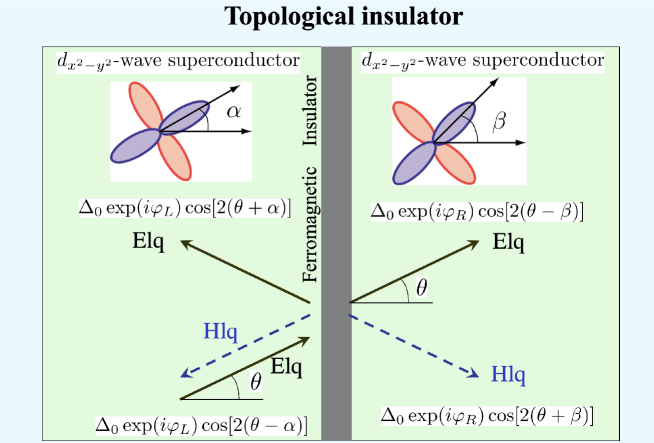
Figure 1: Schematic illustration of the $d$-wave superconductor junctions on the surface of a 3D topological insulator (TI). An electron-like quasiparticle (Elq) is injected and it is reflected or transmitted as Elq and hole-like quasiparticle (Hlq). $\Delta_{L+}(\theta)=\Delta_{0}\cos\left[2\left(\theta-\alpha\right)\right]\exp(i\varphi)$ and $\Delta_{R+}(\theta)=\Delta_{0}\cos\left[2\left(\theta-\beta\right)\right]$ are pair potentials felt by quasiparticle with the direction $\theta$, where the angle $\theta$ is measured from the normal to the interface. $\Delta_{L-}(\theta)=\Delta_{0}\cos\left[2\left(\theta+\alpha\right)\right]\exp(i\varphi)$ and $\Delta_{R-}(\theta)=\Delta_{0}\cos\left[2\left(\theta+\beta\right)\right]$ are pair potentials felt by quasiparticle with the direction $\pi-\theta$, where the angle $\theta$ is measured from the normal to the interface.

II.2 Wave functions of BdG equation

A BdG wave function of the above Hamiltonian is given by

$$\Psi\left(\bm{x}\right)=\exp\left(ik_{Fy}y\right)\left[\Psi_{SL}\left(x\right)\Theta\left(-x\right)+\Psi_{FI}\left(x\right)\Theta\left(x\right)\Theta\left(d-x\right)+\Psi_{SR}\left(x\right)\Theta\left(x-d\right)\right]$$

with the momentum parallel to the interface $k_{Fy}$. We denote the quasiparticle energy measured from the Fermi surface as $E$ and assume the conditions where $\mid E\mid\ll\mu$, $\Delta_{0}\ll\mu$, $\mid E\mid\ll\mid m_{z}\mid$, and $\Delta_{0}\ll\mid m_{z}\mid$ are satisfied. If we consider an electron-like quasiparticle injection from the left superconductor, $\Psi_{SL}(x)$, $\Psi_{FI}(x)$, and $\Psi_{SR}(x)$ are given by

$$\Psi_{SL}\left(x\right) = \left(\Psi^{e}_{in}\!+\!a_{e}\Psi_{hr}\right)\exp\left(ik_{Fx}x\right)+b_{e}\Psi_{er}\exp\left(-ik_{Fx}x\right),$$ (II.3)

$$\Psi_{FI}\left(x\right) = f_{1e}\Psi_{e1}\exp\left(-\kappa_{ex}x\right)+f_{2e}\Psi_{e2}\exp\left(\kappa_{ex}x\right)$$ (II.4)

$$+f_{3e}\Psi_{h1}\exp\left(\kappa_{hx}x\right)+f_{4e}\Psi_{h2}\exp\left(-\kappa_{hx}x\right),$$

$$\Psi_{SR}\left(x\right) = c_{e}\Psi_{et}\exp\left(ik_{Fx}x\right)+d_{e}\Psi_{ht}\exp\left(-ik_{Fx}x\right),$$ (II.5)

$$k_{Fx}=\sqrt{\left(\mu/v\right)^{2}-k_{Fy}^{2}},\ \ \kappa_{ex}=\kappa_{hx}=\sqrt{m_{z}^{2}+v^{2}k_{y}^{2}}/v.$$

$\Psi^{e}_{in}$, $\Psi_{hr}$, $\Psi_{er}$ defined in the left superconductor are given by

$$\Psi^{e}_{in}=\begin{pmatrix}1\\ \exp\left(i\theta\right)\\ -\Gamma_{L+}\exp\left[i\left(\theta-\varphi\right)\right]\\ \Gamma_{L+}\exp\left(-i\varphi\right)\\ \end{pmatrix},\ \ \Psi_{hr}=\begin{pmatrix}\Gamma_{L+}\\ \Gamma_{L+}\exp\left(i\theta\right)\\ -\exp\left[i\left(\theta-\varphi\right)\right]\\ \exp\left(-i\varphi\right)\end{pmatrix},\ \ \Psi_{er}=\begin{pmatrix}1\\ -\exp\left(-i\theta\right)\\ \Gamma_{L-}\exp\left[-i\left(\theta+\varphi\right)\right]\\ \Gamma_{L-}\exp\left(-i\varphi\right)\end{pmatrix}$$ (II.6)

with $\exp(i\theta)=(k_{Fx}+ik_{Fy})/k_{F}$. $\Psi_{e1}$, $\Psi_{e2}$, $\Psi_{h1}$, and $\Psi_{h2}$ in FI are

$$\Psi_{e1}=\begin{pmatrix}i\gamma\\ 1\\ 0\\ 0\end{pmatrix},\ \ \Psi_{e2}=\begin{pmatrix}-i\gamma^{-1}\\ 1\\ 0\\ 0\end{pmatrix},\Psi_{h1}=\begin{pmatrix}0\\ 0\\ i\gamma\\ 1\end{pmatrix},\Psi_{h2}=\begin{pmatrix}0\\ 0\\ -i\gamma^{-1}\\ 1\end{pmatrix}$$ (II.7)

$\gamma=-v(\kappa_{ex}-k_{Fy})/m_{z}$. $\Psi_{et}$, $\Psi_{ht}$ in the right superconductor are given by

$$\Psi_{et}=\begin{pmatrix}1\\ \exp\left(i\theta\right)\\ -\Gamma_{R+}\exp\left(i\theta\right)\\ \Gamma_{R+}\end{pmatrix},\ \ \Psi_{ht}=\begin{pmatrix}\Gamma_{R-}\\ -\Gamma_{R-}\exp\left(-i\theta\right)\\ \exp\left(-i\theta\right)\\ 1\end{pmatrix}$$ (II.8)

with

$$\Gamma_{L\pm}=\frac{\Delta_{L\pm}\left(\theta\right)}{E+\sqrt{E^{2}-\Delta^{2}_{L\pm}\left(\theta\right)}},\ \Gamma_{R\pm}=\frac{\Delta_{R\pm}\left(\theta\right)}{E+\sqrt{E^{2}-\Delta^{2}_{R\pm}\left(\theta\right)}}.$$

We can also calculate the wave function corresponding to eqs. (II.3), (II.4), and (II.5) with hole-like quasiparticle injection as follows.

$$\Psi_{SL}\left(x\right) = \left(\Psi^{h}_{in}\!+\!a_{h}\Psi_{er}\right)\exp\left(-ik_{Fx}x\right)+b_{h}\Psi_{hr}\exp\left(ik_{Fx}x\right),$$ (II.9)

$$\Psi_{FI}\left(x\right) = f_{1h}\Psi_{e1}\exp\left(-\kappa_{ex}x\right)+f_{2h}\Psi_{e2}\exp\left(\kappa_{ex}x\right)$$ (II.10)

$$+f_{3h}\Psi_{h1}\exp\left(\kappa_{hx}x\right)+f_{4h}\Psi_{h2}\exp\left(-\kappa_{hx}x\right),$$

$$\Psi_{SR}\left(x\right) = c_{h}\Psi_{et}\exp\left(ik_{Fx}x\right)+d_{h}\Psi_{ht}\exp\left(-ik_{Fx}x\right),$$ (II.11)

with

$$\Psi^{h}_{in}=\begin{pmatrix}\Gamma_{L-}\\ -\Gamma_{L-}\exp\left(-i\theta\right)\\ \exp\left[-i\left(\theta+\varphi\right)\right]\\ \exp\left(-i\varphi\right)\\ \end{pmatrix}.$$

$\Psi_{SL}(x)$, $\Psi_{FI}(x)$, and $\Psi_{SR}(x)$ satisfy the boundary conditions $\Psi_{SL}(x=0)=\Psi_{FI}(x=0)$ and $\Psi_{FI}(x=d)=\Psi_{SR}(x=d)$. The Andreev reflection coefficients $a_{e}$ and $a_{h}$ are needed to calculate Josephson current Furusaki and Tsukada (1991a); Tanaka and Kashiwaya (1996a). They are given by

$$a_{e}=-\frac{\sigma_{N}\Lambda_{1e}+\left(1-\sigma_{N}\right)\Lambda_{2e}}{\Lambda_{d}(E,\theta)},\ \ a_{h}=-\frac{\sigma_{N}\Lambda_{1h}+\left(1-\sigma_{N}\right)\Lambda_{2h}}{\Lambda_{d}(E,\theta)}$$ (II.12)

with

$$\Lambda_{d}\left(E,\theta\right) = \left[1-\sigma_{N}\right]\left[1+\exp\left(-i\eta\right)\Gamma_{R+}\Gamma_{R-}\right]\left[1+\exp\left(i\eta\right)\Gamma_{L+}\Gamma_{L-}\right]$$ (II.13)

$$+ \sigma_{N}\left[1-\exp\left(-i\varphi\right)\Gamma_{L-}\Gamma_{R-}\right]\left[1-\exp\left(i\varphi\right)\Gamma_{L+}\Gamma_{R+}\right]$$

$$\Lambda_{1e} = \left[1-\exp(-i\varphi)\Gamma_{L-}\Gamma_{R-}\right]\left[\Gamma_{L+}-\Gamma_{R+}\exp\left(i\varphi\right)\right]$$

$$\Lambda_{2e} = \left[1+\exp(-i\eta)\Gamma_{R+}\Gamma_{R-}\right]\left[\Gamma_{L+}+\exp\left(i\eta\right)\Gamma_{L-}\right]$$ (II.14)

$$\Lambda_{1h} = \left[1-\exp(i\varphi)\Gamma_{L+}\Gamma_{R+}\right]\left[\Gamma_{L-}-\Gamma_{R-}\exp\left(-i\varphi\right)\right]$$

$$\Lambda_{2h} = \left[1+\exp(-i\eta)\Gamma_{R+}\Gamma_{R-}\right]\left[\Gamma_{L-}+\exp(i\eta)\Gamma_{L+}\right]$$ (II.15)

and

$$\cos\eta=\frac{m_{z}^{2}\cos^{2}\theta-\mu^{2}\sin^{2}\theta}{m_{z}^{2}\cos^{2}\theta+\mu^{2}\sin^{2}\theta},\ \ \sin\eta=\frac{-2m_{z}\mu\cos\theta\sin\theta}{m_{z}^{2}\cos^{2}\theta+\mu^{2}\sin^{2}\theta}.$$ (II.16)

Here, $\sigma_{N}$ is the transparency of this junction in the normal state and it is given by

$$\sigma_{N}=\frac{\cos^{2}\theta}{{\rm cosh}^{2}\left(\kappa_{ex}d\right)\cos^{2}\theta+{\rm sinh}^{2}\left(\kappa_{ex}d\right)\sin^{2}\theta\sin^{2}\left(\frac{\eta}{2}\right)}.$$ (II.17)

II.3 Josephson current formula based on Andreev reflection coefficients

Based on the Green’s function of BdG equation, it is known that Josephson current is expressed by $a_{en}$ and $a_{hn}$ which are obtained from the analytical continuation from $E$ to $i\omega_{n}$ in $a_{e}$ and $a_{h}$ for conventional $s$-wave superconductor Furusaki and Tsukada (1991a), $d$-wave superconductor Tanaka and Kashiwaya (1996a, 1997), and junctions on the TI Lu et al. (2015); Bo and Yukio (2018), where $\omega_{n}=2\pi k_{B}T(n+1/2)$ is the Matsubara frequency. The resulting Josephson current $I(\varphi)$ is given by Tanaka and Kashiwaya (1996a); Lu et al. (2015); Bo and Yukio (2018)

$$R_{N}I\left(\varphi\right)=\frac{\pi\bar{R}_{N}k_{B}T}{e}\left\{\sum_{\omega_{n}}\int^{\pi/2}_{-\pi/2}\left[\frac{a_{en}\left(\theta,\varphi\right)}{\Omega_{nL+}}\Delta_{L+}\left(\theta\right)-\frac{a_{hn}\left(\theta,\varphi\right)}{\Omega_{nL-}}\Delta_{L-}\left(\theta\right)\right]\cos\theta d\theta\right\}$$ (II.18)

with

$$\bar{R}_{N}^{-1}=\int^{\pi/2}_{-\pi/2}\sigma_{N}\cos\theta d\theta,\ \Omega_{nL\pm}={\rm sgn}\left(\omega_{n}\right)\sqrt{\Delta^{2}_{L}\left(\theta_{\pm}\right)+\omega_{n}^{2}}$$

and

$$a_{en}=i\frac{\sigma_{N}\Lambda_{1en}+\left(1-\sigma_{N}\right)\Lambda_{2en}}{\Lambda_{dn}(\theta,\varphi)},\ \ a_{hn}=i\frac{\sigma_{N}\Lambda_{1hn}+\left(1-\sigma_{N}\right)\Lambda_{2hn}}{\Lambda_{dn}(\theta,\varphi)}$$ (II.19)

with

$$\Lambda_{dn}\left(\theta,\varphi\right) = \left[1-\sigma_{N}\right]\left[1-\exp\left(-i\eta\right)\Gamma_{nR+}\Gamma_{nR-}\right]\left[1-\exp\left(i\eta\right)\Gamma_{nL+}\Gamma_{nL-}\right]$$ (II.20)

$$+ \sigma_{N}\left[1+\exp\left(-i\varphi\right)\Gamma_{nL-}\Gamma_{nR-}\right]\left[1+\exp\left(i\varphi\right)\Gamma_{nL+}\Gamma_{nR+}\right]$$

$$\Lambda_{1en} = \left[1+\exp(-i\varphi)\Gamma_{nL-}\Gamma_{nR-}\right]\left[\Gamma_{nL+}-\Gamma_{nR+}\exp\left(i\varphi\right)\right]$$

$$\Lambda_{2en} = \left[1-\exp(-i\eta)\Gamma_{nR+}\Gamma_{nR-}\right]\left[\Gamma_{nL+}+\exp\left(i\eta\right)\Gamma_{nL-}\right],$$ (II.21)

$$\Lambda_{1hn} = \left[1+\exp(i\varphi)\Gamma_{nL+}\Gamma_{nR+}\right]\left[\Gamma_{nL-}-\Gamma_{nR-}\exp\left(-i\varphi\right)\right]$$

$$\Lambda_{2hn} = \left[1-\exp(-i\eta)\Gamma_{nR+}\Gamma_{nR-}\right]\left[\Gamma_{nL-}+\exp(i\eta)\Gamma_{nL+}\right],$$ (II.22)

with

$$\Gamma_{nL\pm}=\frac{\Delta_{L\pm}\left(\theta\right)}{\omega_{n}+\Omega_{nL\pm}},\ \Gamma_{nR\pm}=\frac{\Delta_{R\pm}\left(\theta\right)}{\omega_{n}+\Omega_{nR\pm}}.$$

By using $\Gamma_{nL\pm}(\theta)=\Gamma_{nL\mp}(-\theta)$, $\Gamma_{nR\pm}(\theta)=\Gamma_{nR\mp}(-\theta)$,

$$R_{N}I(\varphi)=\frac{\pi\bar{R}_{N}k_{B}T}{e}\sum_{n}\int^{\pi/2}_{-\pi/2}d\theta\frac{4\Gamma_{nL+}\Gamma_{nR+}}{\mid\Lambda_{dn}\left(\theta,\varphi\right)\mid^{2}}\cos\theta\sigma_{N}F(\theta,i\omega_{n},\varphi)$$ (II.23)

$$F(\theta,i\omega_{n},\varphi)=\left(1-\sigma_{N}\right)\Lambda_{1n}+\sigma_{N}\sin\varphi\mid 1+\exp\left(i\varphi\right)\Gamma_{nL-}\Gamma_{nR-}\mid^{2}$$ (II.24)

with

$$\Lambda_{1n} = \sin\varphi{\rm Real}\left[\left(1-\exp\left(i\eta\right)\Gamma_{nL+}\Gamma_{nL-}\right)\left(1-\exp\left(-i\eta\right)\Gamma_{nR+}\Gamma_{nR-}\right)\right]$$ (II.25)

$$+ \cos\varphi\sin\eta\left(\Gamma_{nL+}\Gamma_{nL-}-\Gamma_{nR+}\Gamma_{nR-}\right).$$

The obtained $I(\varphi)$ reproduces standard formula of $d$-wave superconductor junctions without a TI Tanaka and Kashiwaya (1996a); Barash et al. (1996); Tanaka and Kashiwaya (1997, 2000) by choosing $\eta=\pi$. In the next section, by using eqs. (II.23) and (II.24), we calculate $I(\varphi)$ and the quality factor $Q$. In order to prove the $m_{z}$, $\alpha$, and $\beta$ dependence of $I(\varphi)$ analytically, it is convenient to transform $F(\theta,i\omega_{n},\varphi)$ in eqs. (II.23) and (II.24) as follows.

$$F(\theta,i\omega_{n},\varphi) = \left(1-\sigma_{N}\right)\left(\sin\varphi\Lambda_{ne}+\cos\varphi\Lambda_{no}\right)$$ (II.26)

$$+ \sigma_{N}\left[\sin\varphi\left(1+\Gamma^{2}_{nL-}\Gamma^{2}_{nR-}\right)+\Gamma_{nL-}\Gamma_{nR-}\sin 2\varphi\right]$$

with

$$\Lambda_{ne}=1+\Gamma_{nL+}\Gamma_{nL-}\Gamma_{nR+}\Gamma_{nR-}-\cos\eta\left(\Gamma_{nL+}\Gamma_{nL-}+\Gamma_{nR+}\Gamma_{nR-}\right),$$ (II.27)

and

$$\Lambda_{no}=\left(\Gamma_{nL+}\Gamma_{nL-}-\Gamma_{nR+}\Gamma_{nR-}\right)\sin\eta.$$ (II.28)

Here, $\Lambda_{ne}$ and $\Lambda_{no}$ are even and odd function of $\theta$, respectively.

III Results

First, let us focus on the current phase relation (CPR). In order to understand the obtained results more intuitively, we rewrite eq. (II.23) as follows,

$$R_{N}I(\varphi)=\frac{\pi\bar{R}_{N}k_{B}T}{e}\sum_{n}\int^{\pi/2}_{-\pi/2}d\theta\frac{2\cos\theta\sigma_{N}}{\mid\Lambda_{dn}\left(\theta,\varphi\right)\mid^{2}}\left[A\left(\theta\right)\sin\varphi+B\left(\theta\right)\sin 2\varphi+C\left(\theta\right)\cos\varphi\right]$$ (III.1)

with

$$A\left(\theta\right)=\left(\Gamma_{nL+}\Gamma_{nR+}+\Gamma_{nL-}\Gamma_{nR-}\right)\left[\left(1-\sigma_{N}\right)\Lambda_{ne}+\sigma_{N}\left(1+\Gamma_{nL+}\Gamma_{nL-}\Gamma_{nR+}\Gamma_{nR-}\right)\right],$$ (III.2)

$$B\left(\theta\right)=2\sigma_{N}\Gamma_{nL+}\Gamma_{nL-}\Gamma_{nR+}\Gamma_{nR-},\ \ C\left(\theta\right)=\left(1-\sigma_{N}\right)\left(\Gamma_{nL+}\Gamma_{nR+}-\Gamma_{nL-}\Gamma_{nR-}\right)\Lambda_{no}$$ (III.3)

using the definition of $\Lambda_{dn}(\theta,\varphi)$, $\Lambda_{ne}$, and $\Lambda_{no}$ given in eqs. (II.20), (II.27) and (II.28). In general, due to the $\varphi$ dependence of $\Lambda_{dn}(\theta,\varphi)$ in eq. (III.1), $I(\varphi)$ includes terms proportional to $\sin(n\varphi)$ and $\cos(n\varphi)$ with $(n\geq 1)$. As seen from eq.III.3, the term which is proportional to $\cos\varphi$ in eq. (III.1) appears when both $\Lambda_{no}\neq 0$ and $\Gamma_{nL+}\Gamma_{nR+}\neq\Gamma_{nL-}\Gamma_{nR-}$ are satisfied except for special $\theta$. This means that $\sin\eta$ in $\Lambda_{no}$ (eq. II.28) and $m_{z}$ in eq. (II.16) are nonzero. It is remarkable that the term proportional to $\cos\varphi$ in eq. (III.1) is induced by $m_{z}$ which is in sharp contrast to the case of $s$-wave superconductor Josephson junction on TI where in-plane magnetic field generates $\cos\varphi$ term Tanaka et al. (2009). However, the magnitude of $m_{z}$ cannot be too large, since the coupling between two superconductors becomes weaker and the magnitude of $\sin(2\varphi)$ term is suppressed since it is basically proportional to the second order of the transparency of the junctions. The coexistence of all three harmonics, $i.e.$, $\sin\varphi$, $\cos\varphi$ and $\sin 2\varphi$, is essential for the Josephson diode effect.

As shown later, the quality factor $Q$ depends sensitively on the angles $\alpha$ and $\beta$. It is noted that $\cos\varphi$ term does not appear for $C(\theta)=0$. By choosing $\eta=\pi$, we reproduce the formula of Josephson current of d-wave junctions without TI Tanaka and Kashiwaya (1996a, 1997). Here, we pick up the particular value of $\alpha=-0.2\pi$ and $\beta=0.09\pi$, where $Q$ is hugely enhanced, and examine the current-phase relation. In this case, all terms proportional to $\sin\varphi$, $\cos\varphi$, and $\cos 2\varphi$ of the same order of magnitudes. At this value of $\alpha$, $\beta$, we obtain quite exotic CPR shown in Fig. 2A.

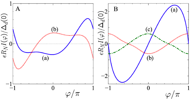
Figure 2: Current phase relation $I(\varphi)$ is plotted for $T=0.05T_{d}$ and $d\mid m_{z}\mid/v=1$. $R_{N}$, $\Delta_{d}(0)$ and $T_{d}$ are the resistance of the junction in the normal state, the amplitude of pair potential at zero temperature, and the transition temperature of $d$-wave superconductor, respectively. A: $\alpha=-0.2\pi$ and $\beta=0.09\pi$. (a)$m_{z}=0.5\mu$, (b)$m_{z}=-0.5\mu$. B: (a)$\alpha=0$, $\beta=0$, and $m_{z}=0.5\mu$. (b)$\alpha=0$, $\beta=0.25\pi$ and $m_{z}=0.5\mu$. (c)$\alpha=0$, $\beta=0.25\pi$ and $m_{z}=-0.5\mu$.

As seen from curves (a) and (b) of Fig. 2A, the magnitude of $I_{c}^{+}$ and $I_{c}^{-}$ are different from each other, where $I_{c}^{+}$ ($I_{c}^{-}$) is the positive (negative) maximum value of $I(\varphi)$. Since the quality factor showing nonreciprocity is expressed by

$$Q=\frac{I_{c}^{+}-\mid I_{c}^{-}\mid}{I_{c}^{+}+\mid I_{c}^{-}\mid},$$ (III.4)

we can expect diode effect for nonzero $Q$. On the other hand, for $\alpha=0$, $\beta=0$ (curve (a) in Fig. 2B) $I(\varphi)$ shows a standard sinusoidal behavior since $\Gamma_{nL+}=\Gamma_{nL-}$, $\Gamma_{nR+}=\Gamma_{nR-}$, and $\Gamma_{nL+}\Gamma_{nR+}=\Gamma_{nL-}\Gamma_{nR-}$ are satisfied. Then, $C(\theta)$ in eq.(III.1) becomes zero and $I(\varphi=0)=I(\varphi=\pi)=0$ is consistent with curve (a) in Fig 2B. For $\alpha=0$, $\beta=\pi/4$, although $I(\varphi)$ shows an unconventional current phase relation with nonzero $I(\varphi)$ at $\varphi=0$, $I_{c}^{+}=\mid I_{c}^{-}\mid$ is still satisfied due to the absence of the term proportional to $\sin\varphi$ in eq. (III.1) since $\Gamma_{nL+}\Gamma_{nR+}+\Gamma_{nL-}\Gamma_{nR-}=0$ is satisfied. Then, $A(\theta)$ in eq.(III.1) becomes zero and the resulting $I(\varphi=\pm\pi/2)=0$ is consistent with curves (b) and (c) in Fig 2B.

By changing the sign of the magnetization from $m_{z}$ to $-m_{z}$, $I(\varphi)=I(\varphi,m_{z})$ satisfies

$$I(\varphi,m_{z})=-I(-\varphi,-m_{z})$$ (III.5)

as seen from curves (a) and (b) in Fig. 2A and curves (b) and (c) in Fig. 2B. This property can be understood from the time reversal operation. Actually, we can show this relation explicitly in the Appendix 1. Next, we show the $\alpha$ and $\beta$ dependence of $Q$ for $-\pi/4\leq\alpha\leq\pi/4$ and $-\pi/4\leq\beta\leq\pi/4$.

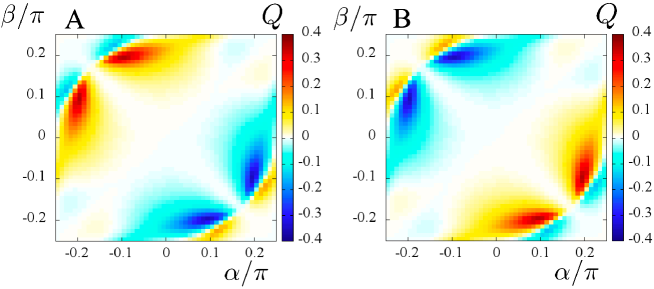
Figure 3: $Q$ is plotted for various $\alpha$ and $\beta$ for $T=0.05T_{d}$ and $d\mid m_{z}\mid/v=1$. (a)$m_{z}=0.5\mu$, (b)$m_{z}=-0.5\mu$.

It is remarkable that the maximum value of $\mid Q\mid$ becomes almost 0.4 and it means the generation of the giant diode effect by tuning $\alpha$ and $\beta$.

Here, by changing $(\alpha,\beta)$ to $(-\alpha,-\beta)$, $Q=Q(\alpha,\beta)$ satisfies

$$Q\left(\alpha,\beta\right)=-Q\left(-\alpha,-\beta\right).$$ (III.6)

We can show this relation analytically as shown in Appendix 2. Also, it can be explained by more intuitive discussion. If we denote the macroscopic phase by $\varphi_{L}$ and $\varphi_{R}$ with $\varphi=\varphi_{L}-\varphi_{R}$ (we set $\varphi_{L}=\varphi$ and $\varphi_{R}=0$ in this model without loosing generality), we have

$$I\left(\varphi,\alpha,\beta\right)=I\left(\varphi_{1},\alpha;\varphi_{2},\beta\right),$$ (III.7)

where the left superconductor has parameters $\left(\varphi_{1},\alpha\right)$ and the right superconductor has $\left(\varphi_{2},\beta\right)$. If we apply a mirror operation with respect to the $yz$ plane, the left superconductor has parameters $\left(\varphi_{2},\beta\right)$ and the right superconductors has $\left(\varphi_{1},\alpha\right)$. Because the direction of the current reverses according to this operation, we have

$$I\left(\varphi_{2},\beta;\varphi_{1},\alpha\right)=-I\left(\varphi_{1},\alpha;\varphi_{2},\beta\right).$$ (III.8)

Therefore, we have

$$I\left(\varphi,\alpha,\beta\right)=-I\left(-\varphi,\beta,\alpha\right).$$ (III.9)

This relation leads to eq. (III.6).

It is interesting to clarify how nonreciprocal effect depends on the temperature. As shown in Fig. 4, $Q$ is enhanced at low temperatures and has a sign change at $T=T_{p}$ with $T_{p}\sim 0.78T_{d}$. Also, there is a sharp peak structure of $Q$ at $T=0.85T_{d}$. This peak structure comes from the intrinsic nature of temperature dependence of $d$-wave superconductor junctions. In $d$-wave superconductor junctions, if we consider injection angle resolved Josephson current, we can decompose into $0$-junction and $\pi$-junction domains. The temperature dependence of Josephson current from $0$-junction domain and that of $\pi$-junction domain can be qualitatively very different shown in previous papers Tanaka and Kashiwaya (1997); Kashiwaya and Tanaka (2000). Then, the macroscopic phase difference $\varphi=\varphi_{m}$. which gives a maximum Josephson current has a jump at some temperature. The resulting maximum Josephson current has a kink like structure as shown in Figs. 36 and 37 in Ref. Kashiwaya and Tanaka (2000). This is the reason why $Q$ has a sharp peak at $T\simeq 0.85T_{d}$.

As shown in curves (a) and (b) in Fig.4A, the overall sign of $Q$ is reversed with the sign change of $m_{z}$.

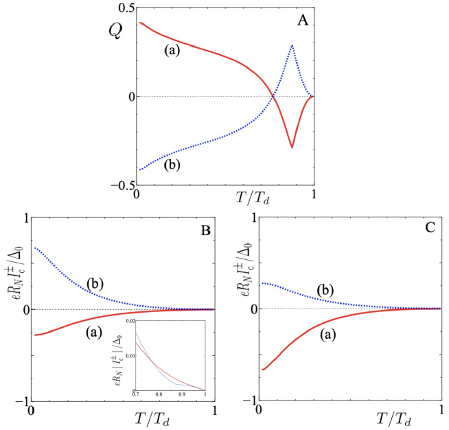
Figure 4: Temperature dependences of $Q$, $I_{c}^{+}$ and $I_{c}^{-}$ are plotted for $\alpha=-0.2\pi$, $\beta=0.09\pi$ and $d\mid m_{z}\mid/v=1$. A: $Q$ for (a)$m_{z}=0.5\mu$, (b)$m_{z}=-0.5\mu$. B: (a)$I_{c}^{-}$ and (b)$I_{c}^{+}$ for $m_{z}=0.5\mu$. In the inset, $\mid I_{c}^{\pm}\mid$ is plotted for $0.7T_{d}<T<T_{d}$. C: (a)$I_{c}^{-}$ and (b)$I_{c}^{+}$ for $m_{z}=-0.5\mu$.

The corresponding $I_{c}^{-}$ and $I_{c}^{+}$ are plotted as curves (a) and (b) for $m_{z}=0.5\mu$ in Fig.4B and those for $m_{z}=-0.5\mu$ in Fig.4C. If we denote $m_{z}$ dependence of $I_{c}^{\pm}$ explicitly, $I_{c}^{\mp}(m_{z}=0.5\mu)=-I_{c}^{\pm}(m_{z}=-0.5\mu)$ to be consistent with eq. (III.5). In the inset of Fig.4B, $\mid I_{c}^{\pm}\mid$ is plotted in the enlarged scale from $0.7T_{d}<T<T_{d}$. $I_{c}^{+}=\mid I_{c}^{-}\mid$ is satisfied for $T=T_{p}$ when $Q$ becomes zero as shown in Fig. 4B.

To elucidate the exotic CPR specific to nonreciprocal nature of Josephson current, we focus on its Fourier components. In general, Josephson current is decomposed into

$$I(\varphi)=\sum_{n}\left[I_{n}\sin n\varphi+J_{n}\cos n\varphi\right].$$ (III.10)

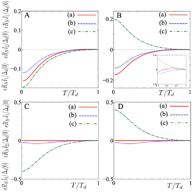
Figure 5: Temperature dependences of (a)$I_{1}$, (b)$I_{2}$ and (c)$J_{1}$ are plotted for $d\mid m_{z}\mid/v=1$. A: $(\alpha,\beta)=(-0.2\pi,0.09\pi)$ with $m_{z}=0.5\mu$, B: $(\alpha,\beta)=(-0.2\pi,0.09\pi)$ with $m_{z}=-0.5\mu$, C: $(\alpha,\beta)=(0,0.25\pi)$ with $m_{z}=0.5\mu$, and D: $(\alpha,\beta)=(0,0.25\pi)$ with $m_{z}=-0.5\mu$. The enlarged plot for $0.7T_{d}<T<T_{d}$ is shown in B as the inset.

For $\alpha=-0.2\pi$ and $\beta=0.09\pi$, $I_{1}$, $I_{2}$, and $J_{1}$ become nonzero values (Figs. 5A and B). By changing $m_{z}$ to $-m_{z}$, $I_{1}$ and $I_{2}$ are invariant and $J_{1}$ has the sign change as shown in Figs. 5A and B. As shown in the inset of Fig. 5B, $I_{1}$ has the sign change at $T=T_{p}$. At this temperature, as shown in Fig. 4A, $Q$ becomes zero. We also show $I_{1}$, $I_{2}$, and $J_{1}$ for $\alpha=0$ and $\beta=0.25\pi$ in Figs. 5C and D. In this case, the resulting $Q$ is zero since the term proportional to $A=A(\theta)$ in eq. (III.1) becomes zero, and the resulting $I_{1}$ becomes zero independent of the sign of $m_{z}$.

Similar to the case for Figs. 5A and B, $I_{2}$ is invariant and $J_{1}$ has a sign change by changing $m_{z}$ to $-m_{z}$. To summarize, the simultaneous existence of $I_{1}$, $I_{2}$ and $J_{1}$ does lead to nonzero $Q$.

Next, we discuss the energy spectrum of the ABSs since it plays a crucial role to determine $I(\varphi)$ Furusaki and Tsukada (1991b); Beenakker and van Houten (1991); Kashiwaya and Tanaka (2000); Löfwander et al. (2001); H. J. Kwon et al. (2004); Tanaka and Kashiwaya (1996b). It is known that the magnitude of $I(\varphi)$ is enhanced at low temperatures due to the presence of low energy ABS. In addition, by the strong spin-momentum locking of the surface states of topological insulator (TI), the ABSs in the present S/FI/S junction become MBSs Fu and Kane (2008); Akhmerov et al. (2009); Law et al. (2009); Tanaka et al. (2009); Linder et al. (2010a). The non-reciprocity, which is responsible for the diode effect, is also apparent in the spectrum of the ABS in the junction.

The energy eigenvalues of ABS(MBS) $E_{b}$ are found by the zero of $\Lambda_{d}(E,\theta)$ defined in eq. (II.13) for

$$\mid E_{b}\mid<{\rm min}\left(\mid\Delta_{L+}\mid,\mid\Delta_{L-}\mid,\mid\Delta_{R+}\mid,\mid\Delta_{R-}\mid\right).$$ (III.11)

Only for limited cases, we can obtain the energy level of $E_{b}$ analytically. For $\alpha=\beta=0$, the energy level of the ABS is expressed by

$$E_{b}=\pm\sqrt{\sigma_{N}\cos^{2}\frac{\varphi}{2}+\left(1-\sigma_{N}\right)\sin^{2}\frac{\eta}{2}}\mid\cos 2\theta\mid\Delta_{0}$$ (III.12)

with

$$\cos^{2}\frac{\eta}{2}=\frac{m_{z}^{2}\cos^{2}\theta}{m_{z}^{2}\cos^{2}\theta+\mu^{2}\sin^{2}\theta},\ \ \ \sin^{2}\frac{\eta}{2}=\frac{\mu^{2}\sin^{2}\theta}{m_{z}^{2}\cos^{2}\theta+\mu^{2}\sin^{2}\theta}$$

to be consistent with the result of an $s$-wave superconductor junction Tanaka et al. (2009). $E_{b}$ becomes zero for $\varphi=\pm\pi$ and $\theta=0$.

For $\alpha=\beta=\pi/4$, $E_{b}$ becomes

$$E_{b}=\pm\sqrt{\sigma_{N}\cos^{2}\frac{\varphi}{2}+\left(1-\sigma_{N}\right)\cos^{2}\frac{\eta}{2}}\mid\sin 2\theta\mid\Delta_{0}.$$ (III.13)

$E_{b}$ is zero for $\varphi=\pm\pi$ and $\theta=\pm\pi/2$ or $\varphi=\pm\pi$ and $\theta=0$. In this case, the pair potential also becomes zero and $E_{b}$ is absorbed into the continuum level. In these two cases with eqs. (III.12), and (III.13), since $E_{b}$ is a symmetric function of $\varphi$, we can not expect diode effect and resulting $Q$ is zero.

In other cases, only for $\theta=0$ and $\varphi=\pi$, we can show $E_{b}=0$ for wide variety of parameters with $-\pi/4<\alpha<\pi/4$ and $-\pi/4<\beta<\pi/4$. In this case, $\Gamma_{L+}=\Gamma_{L-}=\Gamma_{L}$ and $\Gamma_{R+}=\Gamma_{R-}=\Gamma_{R}$ are satisfied. Then, $\Lambda_{d}(E,\theta)$ becomes

$$\Lambda_{d}\left(E,\theta=0\right)=\left(1-\sigma_{N}\right)\left(1+\Gamma^{2}_{R}\right)\left(1+\Gamma^{2}_{L}\right)+\sigma_{N}\left(1+\Gamma_{L}\Gamma_{R}\right)^{2}.$$ (III.14)

Since $\cos(2\alpha)$ and $\cos(2\beta)$ become positive numbers, $\Gamma_{R}$ and $\Gamma_{L}$ become $-i$ at $E=0$ and $\Lambda_{d}(E,\theta)=0$ at this condition. This means $E_{b}=0$ and the ubiquitous presence of the zero energy ABS for various $\alpha$ and $\beta$ at $\varphi=\pm\pi$ and $\theta=0$.

In general, it is impossible to solve $E_{b}$ analytically, and we plot inverse of $\Lambda_{d}(E,\theta)=\Lambda_{d}(E,\theta,\varphi)$

$$S(E,\theta,\varphi)=\frac{1}{\mid\Lambda_{d}\left(E,\theta,\varphi\right)\mid}.$$ (III.15)

The intensity plot of $S(E,\theta,\varphi)$ for fixed $\varphi$ is shown in Fig. 6. In the actual calculation we replace $E$ with $E+i\delta$ with a small number $\delta=0.001\Delta_{0}$ to avoid the divergence, where we have used the value of $\Delta_{0}$ at zero temperature.

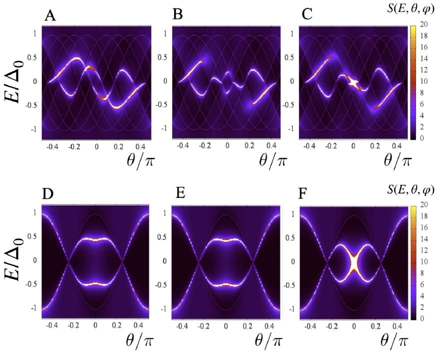
Figure 6: The intensity plot of $S(E,\theta,\varphi)$ for fixed $\varphi$ for $d\mid m_{z}\mid/v=1$ and $m_{z}=0.5\mu$. $(\alpha,\beta)=(-0.2\pi,0.09\pi)$ for A, B and C. $(\alpha,\beta)=(0,0.25\pi)$ for D, E and F. A: $\varphi=0.5\pi$, B: $\varphi=-0.5\pi$, and C: $\varphi=\pi$. D: $\varphi=0.5\pi$, E: $\varphi=-0.5\pi$, and F: $\varphi=\pi$. We plot $\pm\Delta_{0}\cos[2(\theta\pm\alpha)]$ and $\pm\Delta_{0}\cos[2(\theta\pm\beta)]$ as auxiliary lines.

We first show the contour plot of $S(E,\theta,\varphi)$ for fixed value of $\varphi$. The blight curve satisfying eq. (III.11) corresponds to the position of $E_{b}$. As shown in Fig. 6A, $S(E,\theta,\varphi)$ shows a complicated $\theta$ dependence for $\alpha=-0.2\pi$ and $\beta=0.09\pi$ where nonreciprocal effect is prominent as discussed in Figs. 2, 3 and 4. By changing $\varphi=0.5\pi$ to $-0.5\pi$, $S(E,\theta,\varphi)$ shows a dramatically different behavior as shown in Fig.6B as compared to that in Fig.6A. From Figs. 6A and 6B, we see that the ABS energy spectrum is different for the phase biases $\varphi$ ad $-\varphi$ in the regime of the Josephson diode effect. For $\varphi=\pi$, $S(E=0,\theta,\varphi)$ is enhanced around $\theta=0$ (Fig.6C) due to the existence of ABS at $E=0$. For all cases (Figs.6A, 6B and 6C),

$$S(E,\theta,\varphi)\neq S(E,-\theta,\varphi)$$ (III.16)

is satisfied.

On the other hand, for $\alpha=\beta=0$, $S(E,\theta,\varphi)$ shows a symmetric function with $\theta$ (Figs. 6D, E and F)

$$S(E,\theta,\varphi)=S(E,-\theta,\varphi),\ S(E,\theta,\varphi)=S(E,\theta,-\varphi)$$ (III.17)

to be consistent with eq. (III.12).

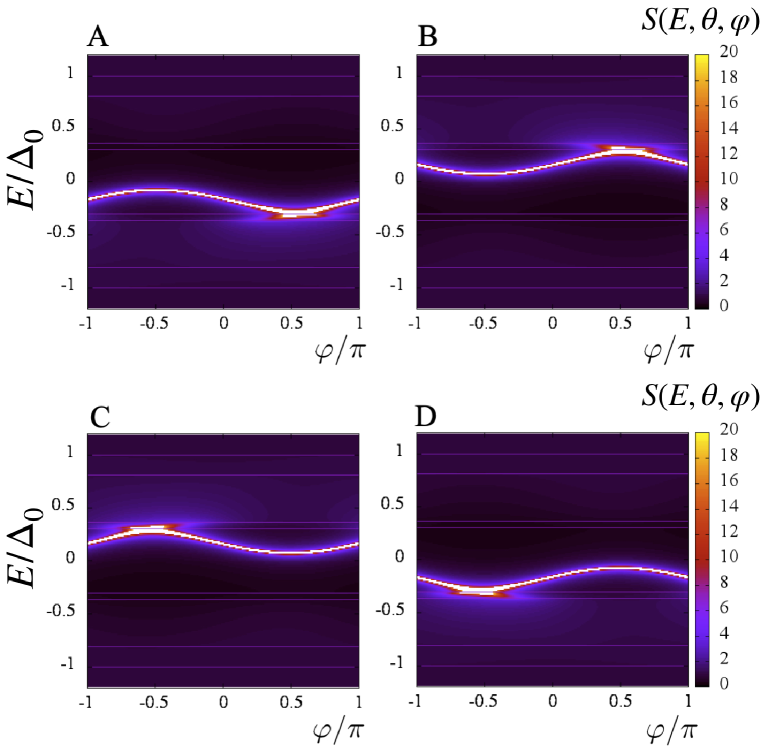
Figure 7: The intensity plot of $S(E,\theta,\varphi)$ for fixed $\theta$ for $d\mid m_{z}\mid/v=1$, $\alpha=-0.2\pi$ and $\beta=0.09\pi$. A: $\theta=0.1\pi$ and $m_{z}=0.5\mu$, B: $\theta=-0.1\pi$ and $m_{z}=0.5\mu$, C: $\theta=0.1\pi$ and $m_{z}=-0.5\mu$, and D: $\theta=-0.1\pi$ and $m_{z}=-0.5\mu$. We plot $\pm\Delta_{0}\cos[2(\theta\pm\alpha)]$ and $\pm\Delta_{0}\cos[2(\theta\pm\beta)]$ as auxiliary lines.

In Fig. 7, we focus on $\varphi$ dependence of $S(E,\theta,\varphi)$ for fixed $\theta$ with $\alpha=-0.2\pi$ and $\beta=0.09\pi$. By changing $\theta$ to $-\theta$, $S(E,\theta,\varphi)$ has a dramatic change. ABS is located for $E<0$ for $\theta=0.1\pi$ while it is located for $E>0$ for $\theta=-0.1\pi$ (Figs. 7A and B). On the other hand, if we change $m_{z}=0.5\mu$ to $m_{z}=-0.5\mu$, ABS is located for $E>0$ for $\theta=0.1\pi$ while it is located for $E<0$ for $\theta=-0.1\pi$ (Figs. 7C and D). It is noted that the non-reciprocal current phase relation of $I(\varphi)$ in Fig. 2A comes from the exotic $\varphi$ dependence of ABS as shown from $S(E,\theta,\varphi)$ in Fig.7. Since $Q$ is determined by the maximum Josephson current, its value can be enhanced by the asymmetric energy spectrum of ABS for $\varphi$ and $-\varphi$.

Finally, we mention how the energy level of $E_{b}$ changes by the transformation from $m_{z}$ to $-m_{z}$. By using the properties of $\Gamma_{R\pm}$, $\Gamma_{L\pm}$, and $\eta$, $\Lambda(E,\theta,\varphi)=\Lambda(E,\theta,\varphi,m_{z})$ and $S(E,\theta,\varphi)=S(E,\theta,\varphi,m_{z})$ satisfy

$$\Lambda_{d}\left(E,-\theta,\varphi,-m_{z}\right) = \left[1-\sigma_{N}\right]\left[1+\exp\left(-i\eta\right)\Gamma_{R+}\Gamma_{R-}\right]\left[1+\exp\left(i\eta\right)\Gamma_{L+}\Gamma_{L-}\right]$$ (III.18)

$$+ \sigma_{N}\left[1-\exp\left(-i\varphi\right)\Gamma_{L+}\Gamma_{R+}\right]\left[1-\exp\left(i\varphi\right)\Gamma_{L-}\Gamma_{R-}\right],$$

$$\Lambda_{d}\left(E,-\theta,-\varphi,-m_{z}\right)=\Lambda_{d}\left(E,\theta,\varphi,m_{z}\right)$$ (III.19)

and

$$S\left(E,-\theta,-\varphi,-m_{z}\right)=S\left(E,\theta,\varphi,m_{z}\right).$$ (III.20)

We can see eq.(III.20) by comparing Fig.7A (7B) and Fig. 7D (7C).

In order to understand the contribution of the zero energy Andreev bound states (ZEABS) to Josephson current, in Fig. 8, we plot $S(0,\theta,\varphi)$ and the magnitude of the angle-resolved Josephson current $\mid I(\theta,\varphi)\mid$ with the same parameters used in Fig.6. For the corresponding $\theta$ and $\varphi$ hosting ZEABS, the resulting $S(E=0,\theta,\varphi)$ is enhanced. Clearly, $\mid I(\theta,\varphi)\mid$ is enhanced for $\theta$ and $\varphi$ when $S(0,\theta,\varphi)$ shows the prominent peak structure. Thus, the ZESAB and the angle resolved Josephson current has a correspondence.

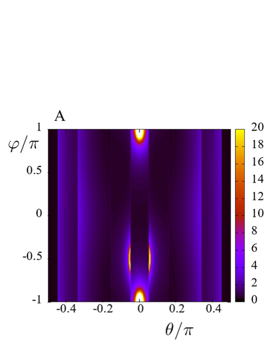
Figure 8: The intensity plot of $S(0,\theta,\varphi)$ for $(\alpha,\beta)=(-0.2\pi,0.09\pi)$ in A. The angle resolved Josephson current $I(\theta,\varphi)$ = $\mid I(\theta,\varphi,\alpha,\beta)\mid$ is plotted in B. We choose $d\mid m_{z}\mid/v=1$, $\alpha=-0.2\pi$, $\beta=0.09\pi$ and $m_{z}=0.5\mu$.

It is known from the study of $d$-wave superconductor junctions in the context of high T_c cuprate, in the presence of the ZESABS, the Josephson current at low temperature is mainly carried by ZESABS Tanaka and Kashiwaya (1996a, 1997). It can trigger non-monotonic temperature dependence of Josephson current observed in high Tc cuprate Testa et al. (2005). The sophisticated $\theta$ and $\varphi$ dependence of $E_{b}(\theta,\varphi)$ in the present $d/FI/d$ junctions on TI shown in Figs. 6, 7 and 8, is due to the breaking of $\cal{P}$ and $\cal{T}$ symmetry, and generates the exotic current phase relation with simultaneous coexistence of $\sin\varphi$, $\sin 2\varphi$ and $\cos\varphi$ terms.

IV Conclusions and Discussions

In this paper, we have shown a very large nonreciprocity of Josephson current in a $d$-wave superconductor / Ferromagnetic insulator (FI) / $d$-wave superconductor junction on topological insulator. We have found the large magnitude of quality factor $Q$ which characterizes the diode effect by tuning the crystal axis of both left and right $d$-wave superconductors.

The magnitude of $Q$ becomes almost 0.4 at low temperatures and its sign is reversed by changing the direction of the magnetization in the FI. The physical origin of the large $Q$ stems from the exotic current-phase relations of the Josephson current due to the simultaneous existence of $\sin\varphi$, $\cos\varphi$ and $\sin 2\varphi$ component. The present situation is realized due to the strong asymmetry of the mirror inversion symmetry along the junction interface and the time reversal symmetry breaking by FI. The strong temperature dependence of $Q$ stems from the existence of the low energy Andreev bound state appearing as Majorana bound states (MBSs) at the interface. We have analyzed the Fourier components of Josephson current and found that the $\cos\varphi$ changes sign by the inversion of $m_{z}$. These results can serve as a guide to design Josephson diode using MBSs on the surface of TI.

In this paper, we consider a two-dimensional (2D) junction. It is noted that the present diode effect does not exist in the 1D system. In this case, only the contribution from $\theta$=0 remains in the integral of $\theta$ in eq. (III.1). Since we are considering even-parity superconductor, $\Gamma_{nL+}=\Gamma_{nL-}$ and $\Gamma_{nR+}=\Gamma_{nR-}$ are satisfied at $\theta=0$. Then, $C(\theta=0)$ in eq. (III.3) becomes zero and the resulting $I(\varphi)$ does not have a $\cos\varphi$ dependence. Then, we can not expect the present diode effect.

In the end, we mention the feasibility of the actual experiments. The fabrication of the junction with misorientation angles $\alpha\neq 0$ and $\beta\neq 0$ were realized in high $T_{c}$ cuprate to prove the $d$-wave nature of pairing Tsuei et al. (1994); Tsuei and Kirtley (2000). Also non-monotonic temperature dependence of the maximum Josephson current due to the enhanced $\sin 2\varphi$ component was observed experimentally for $\alpha=-\beta\neq 0$ Il’ichev et al. (2001); Testa et al. (2005). On the other hand, Josephson current was observed in conventional $s$-wave superconductor junctions fabricated on the surface of TIs Veldhorst et al. (2012); Williams et al. (2012); Finck et al. (2014); Kurter et al. (2015). It is noted that $4\pi$ periodicity due to the Kramers pair of MBS was reported Wiedenmann et al. (2016). Furthermore, a high $T_{c}$ cuprate (Bi-2212) /TI junction was fabricated Zareapour et al. (2012). Based on these accumulated experimental works, the realization of the set-up in our proposal seems to be feasible, and our prediction can be tested in the near future. Finally, to pursue superconducting diode effect in the Josepshon junctions with topological superconductors is an interesting future issue Tanaka et al. (2012).

V Appndix 1

In this section, we show eq. (III.5). We can show this relation analytically from eqs. (II.23) and (II.26). Since $\mid\Lambda_{dn}(\theta,\varphi)\mid^{2}=\mid\Lambda_{dn}(-\theta,\varphi)\mid^{2}$ is satisfied. $I(\varphi)$ is expressed in eq. III.1. Here $A(\theta)=A(-\theta)$, $B(\theta)=B(-\theta)$, and $C(\theta)=C(-\theta)$ are satisfied. Since $\exp(-i\eta)$ changes into $\exp(i\eta)$ by the transformation of $\theta$ to $-\theta$ or $m_{z}$ to $-m_{z}$, $\Lambda_{dn}(\theta,\varphi)=\Lambda_{dn}(\theta,m_{z},\varphi)$ satisfies

$$\Lambda_{dn}\left(\theta,-m_{z},\varphi\right)=\Lambda_{dn}\left(-\theta,m_{z},-\varphi\right),\ \Lambda_{dn}\left(-\theta,m_{z},\varphi\right)=\Lambda_{dn}^{*}\left(\theta,m_{z},\varphi\right)$$

and

$$\mid\Lambda_{dn}\left(\theta,-m_{z},\varphi\right)\mid^{2}=\mid\Lambda_{dn}\left(\theta,m_{z},-\varphi\right)\mid^{2}.$$ (V.1)

Also, $\Lambda_{ne}=\Lambda_{ne}(\theta,m_{z})$ and $\Lambda_{no}=\Lambda_{no}(\theta,m_{z})$ satisfy

$$\Lambda_{ne}\left(\theta,m_{z}\right)=\Lambda_{ne}\left(\theta,-m_{z}\right),\ \Lambda_{no}\left(\theta,m_{z}\right)=-\Lambda_{no}\left(\theta,-m_{z}\right).$$

Then, $A(\theta)=A(\theta,m_{z})$, $B(\theta)=B(\theta,m_{z})$, and $C(\theta)=C(\theta,m_{z})$ satisfy

$$A\left(\theta,m_{z}\right)=A\left(\theta,-m_{z}\right),\ B\left(\theta,m_{z}\right)=B\left(\theta,-m_{z}\right),\ C\left(\theta,m_{z}\right)=-C\left(\theta,-m_{z}\right).$$

As a result, we can derive eq. (III.5).

VI Appendix 2

We can show eq. (III.6) as follows. Since $\Gamma_{nL\pm}$ and $\Gamma_{nR\pm}$ change into $\Gamma_{nL\mp}$ and $\Gamma_{nR\mp}$ by the transformation $(\alpha,\beta)$ to $(-\alpha,-\beta)$, $\Lambda_{dn}(\theta,\varphi)=\Lambda_{dn}(\theta,\varphi,\alpha,\beta)$, $\Lambda_{ne}=\Lambda_{ne}(\theta,\alpha,\beta)$, and $\Lambda_{no}=\Lambda_{no}(\theta,\alpha,\beta)$ in eqs. (II.20), (II.27), and (II.28) satisfy

$$\Lambda_{dn}\left(\theta,\varphi,-\alpha,-\beta\right)=\Lambda_{dn}\left(\theta,-\varphi,\alpha,\beta\right),$$ (VI.1)

and

$$\Lambda_{ne}\left(\theta,-\alpha,-\beta\right)=\Lambda_{ne}\left(\theta,\alpha,\beta\right),\ \ \Lambda_{no}\left(\theta,-\alpha,-\beta\right)=\Lambda_{no}\left(\theta,\alpha,\beta\right).$$ (VI.2)

If we write $\alpha$, $\beta$ dependence of $I(\varphi)$ explicitly,

$$I\left(\varphi,\alpha,\beta\right)=-I\left(-\varphi,-\alpha,-\beta\right)$$ (VI.3)

is obtained and it leads to eq. (III.6).

VII Appendix3

In this Appendix, we explain why simple $d$-wave superconductor junctions by cuprate without TI does not show any diode effet. In $d$-wave / ferromagnet insulator /$d$-wave superconductor junction, there is no diode effect since $\cos\varphi$ term is not generated as shown in Ref. Tanaka and Kashiwaya (2000) if the spin-orbit coupling is absent. We can prove why d/FI/d junction without TI can not hold the diode effect. The Hamiltonian in $d$-wave junctions realized in cuprates is given by

$$\left[\begin{array}[]{cccc}-\frac{\hbar^{2}\left(\partial_{x}^{2}+\partial_{y}^{2}\right)}{2m}-\mu+m_{z}&0&0&\Delta\left(k_{x},k_{y}\right)e^{i\varphi}\\ 0&-\frac{\hbar^{2}\left(\partial_{x}^{2}+\partial_{y}^{2}\right)}{2m}-\mu-m_{z}&-\Delta\left(k_{x},k_{y}\right)e^{i\varphi}&0\\ 0&-\Delta\left(k_{x},k_{y}\right)e^{-i\varphi}&\frac{\hbar^{2}\left(\partial_{x}^{2}+\partial_{y}^{2}\right)}{2m}+\mu-m_{z}&0\\ \Delta\left(k_{x},k_{y}\right)e^{-i\varphi}&0&0&\frac{\hbar^{2}\left(\partial_{x}^{2}+\partial_{y}^{2}\right)}{2m}+\mu+m_{z}\end{array}\right],$$ (VII.1)

with

$$\Delta\left(k_{x},k_{y}\right)=\left(\hat{k}_{x}^{2}-\hat{k}_{y}^{2}\right)\cos 2\alpha-2\hat{k}_{x}\hat{k}_{y}\sin 2\alpha.$$ (VII.2)

The time reversal symmetry is

$$T=\left[\begin{array}[]{cc}is_{y}K&0\\ 0&is_{y}K\end{array}\right],$$ (VII.3)

and another relevant operator is the $C_{2y}$ given by

$$C_{2y}=\left[\begin{array}[]{cc}e^{-i\frac{\pi}{2}s_{y}}&0\\ 0&e^{-i\frac{\pi}{2}s_{y}}\end{array}\right]=\left[\begin{array}[]{cc}-is_{y}&0\\ 0&-is_{y}\end{array}\right].$$ (VII.4)

Let us define a combined operator $\tilde{T}$

$$\tilde{T}=TC_{2y}=\left[\begin{array}[]{cc}-s_{0}K&0\\ 0&-s_{0}K\end{array}\right],$$ (VII.5)

we can obtain

$$\tilde{T}H\left(\varphi\right)\tilde{T}^{-1}=H\left(-\varphi\right).$$ (VII.6)

It implies that the energy spectrum has symmetry

$$E_{n}\left(\varphi\right)=E_{n}\left(-\varphi\right).$$ (VII.7)

The energy of the junction is an even function of the phase difference $\varphi$. Thus, the Josephson current is an odd function of $\varphi$ according to

$$I\left(\varphi\right)=\frac{2e}{\hbar}\frac{\partial F}{\partial\varphi}=\frac{2e}{\hbar}\frac{\partial}{\partial\varphi}\left(\sum\nolimits_{n}E_{n}\left(\varphi\right)f_{n}\right),$$ (VII.8)

$$I\left(-\varphi\right)=\frac{2e}{\hbar}\frac{\partial F}{\partial\varphi}=\frac{2e}{\hbar}\frac{\partial}{\partial\varphi}\left(\sum\nolimits_{n}E_{n}\left(-\varphi\right)f_{n}\right)=-I\left(\varphi\right)$$ (VII.9)

with Fermi distribution function $f_{n}$. Then, we can get

$$I\left(-\varphi\right)=-I\left(\varphi\right),$$ (VII.10)

and

$$I\left(0\right)=0.$$ (VII.11)

If $I\left(0\right)=0$, the Josephson current can not hold $\cos\varphi$ term which is required by diode effect. We can therefore conclude that the similar d/FI/d junction without TI can not harbor diode effect due to the combined $\tilde{T}$ symmetry. Instead, if there is spin-orbit couplings, $\tilde{T}H\left(\varphi\right)\tilde{T}^{-1}$ will no longer equal to $H\left(-\varphi\right)$, then we can expect the $\cos\varphi$ term and diode effect. The presence of spin-orbit coupling is essential for the diode effect.

On the other hand, the surface state of a topological insulator has a strong spin-orbit coupling which generates spin-momentum locking. To enhance $\cos\varphi$ term, it is promising to consider $d/FI/d$ junction on the surface of TI.

References

- Tokura and Nagaosa (2018) Y. Tokura and N. Nagaosa, Nat. Commun. 9, 3740 (2018).
- Rikken et al. (2001) G. L. J. A. Rikken, J. Fölling, and P. Wyder, Phys. Rev. Lett. 87, 236602 (2001).
- Krstić et al. (2002) V. Krstić, S. Roth, M. Burghard, K. Kern, and G. L. J. A. Rikken, J. Chem. Phys. 117, 11315 (2002).
- Pop et al. (2014) F. Pop, P. Auban-Senzier, E. Canadell, G. L. J. A. Rikken, and N. Avarvari, Nat. Commun. 5, 3757 (2014).
- Rikken and Wyder (2005) G. L. J. A. Rikken and P. Wyder, Phys. Rev. Lett. 94, 016601 (2005).
- Ideue et al. (2017) T. Ideue, K. Hamamoto, S. Koshikawa, M. Ezawa, S. Shimizu, Y. Kaneko, Y. Tokura, N. Nagaosa, and Y. Iwasa, Nat. Phys. 13, 578 (2017).
- Hoshino et al. (2018) S. Hoshino, R. Wakatsuki, K. Hamamoto, and N. Nagaosa, Phys. Rev. B 98, 054510 (2018).
- Wakatsuki et al. (2017) R. Wakatsuki, Y. Saito, S. Hoshino, Y. M. Itahashi, T. Ideue, M. Ezawa, Y. Iwasa, and N. Nagaosa, Sci. Adv. 3, e1602390 (2017).
- Qin et al. (2017) F. Qin, W. Shi, T. Ideue, M. Yoshida, A. Zak, R. Tenne, T. Kikitsu, D. Inoue, D. Hashizume, and Y. Iwasa, Nat. Commun. 8, 14465 (2017).
- Itahashi et al. (2020) Y. M. Itahashi, T. Ideue, Y. Saito, S. Shimizu, T. Ouchi, T. Nojima, and Y. Iwasa, Sci. Adv. 6, eaay9120 (2020).
- Ando et al. (2020) F. Ando, Y. Miyasaka, T. Li, J. Ishizuka, T. Arakawa, Y. Shiota, T. Moriyama, Y. Yanase, and T. Ono, Nature 584, 373 (2020).
- Pal et al. (2022) B. Pal, A. Chakraborty, P. K. Sivakumar, M. Davydova, A. K. Gopi, A. K. Pandeya, J. A. Krieger, Y. Zhang, M. Date, S. Ju, N. Yuan, N. B. M. Schroter, L. Fu, and S. S. P. Parkin, Nature Physics 18, 1228 (2022).
- Narita et al. (2022) H. Narita, J. Ishizuka, R. Kawarazaki, D. Kan, Y. Shiota, T. Moriyama, Y. Shimakawa, A. V. Ognev, A. S. Samardak, Y. Yanase, and T. Ono, Nature Nanotechnology 17, 823 (2022).
- Jeon et al. (2022) K.-R. Jeon, J.-K. Kim, J. Yoon, J.-C. Jeon, H. Han, A. Cottet, T. Kontos, and S. S. P. Parkin, Nature Materials 21, 1008 (2022).
- Bauriedl et al. (2022) L. Bauriedl, C. B”auml, L. Fuchs, C. Baumgartner, N. Paulik, J. M. Bauer, K.-Q. Lin, J. M. Lupton, T. Taniguchi, K. Watanabe, C. Strunk, and N. Paradiso, Nature Communications 13, 4266 (2022).
- He et al. (2022) J. J. He, Y. Tanaka, and N. Nagaosa, New J. Phys. 24, 053014 (2022).
- Daido et al. (2022) A. Daido, Y. Ikeda, and Y. Yanase, Phys. Rev. Lett. 128, 037001 (2022).
- Yuan and Fu (2022) N. F. Q. Yuan and L. Fu, Proc. Nat. Acad. of Sci. 119, e2119548119 (2022).
- Ilić and Bergeret (2022) S. Ilić and F. S. Bergeret, Phys. Rev. Lett. 128, 177001 (2022).
- Karabassov et al. (2022) T. Karabassov, I. V. Bobkova, A. A. Golubov, and A. S. Vasenko, arXiv:2203.15608 (2022).
- Souto et al. (2022) R. S. Souto, M. Leijnse, and C. Schrade, arXiv:2205.04469 (2022).
- Jiang et al. (2022) J. Jiang, M. Milošević, Y.-L. Wang, Z.-L. Xiao, F. Peeters, and Q.-H. Chen, Phys. Rev. Applied 18, 034064 (2022).
- Daido and Yanase (2022) A. Daido and Y. Yanase, “Superconducting diode effect and nonreciprocal transition lines,” (2022).
- Kokkeler et al. (2022) T. Kokkeler, F. S. Bergeret, and A. Golubov, “Field-free anomalous junction and superconducting diode effect in spin split superconductor/topological insulator junctions,” (2022).
- Misaki and Nagaosa (2021) K. Misaki and N. Nagaosa, Phys. Rev. B 103, 245302 (2021).
- Hu (1994) C.-R. Hu, Phys. Rev. Lett. 72, 1526 (1994).
- Tanaka and Kashiwaya (1995) Y. Tanaka and S. Kashiwaya, Phys. Rev. Lett. 74, 3451 (1995).
- Kashiwaya and Tanaka (2000) S. Kashiwaya and Y. Tanaka, Rep. Prog. Phys. 63, 1641 (2000).
- Löfwander et al. (2001) T. Löfwander, V. S. Shumeiko, and G. Wendin, Supercond. Sci. Technol. 14, R53 (2001).
- Yip (1993) S. Yip, J. Low Temp. Phys. 91, 203 (1993).
- Tanaka and Kashiwaya (1996a) Y. Tanaka and S. Kashiwaya, Phys. Rev. B 53, R11957 (1996a).
- Tanaka and Kashiwaya (1997) Y. Tanaka and S. Kashiwaya, Phys. Rev. B 56, 892 (1997).
- Barash et al. (1996) Y. S. Barash, H. Burkhardt, and D. Rainer, Phys. Rev. Lett. 77, 4070 (1996).
- Testa et al. (2005) G. Testa, E. Sarnelli, A. Monaco, E. Esposito, M. Ejrnaes, D.-J. Kang, S. H. Mennema, E. J. Tarte, and M. G. Blamire, Phys. Rev. B 71, 134520 (2005).
- Tanaka et al. (2009) Y. Tanaka, T. Yokoyama, and N. Nagaosa, Phys. Rev. Lett. 103, 107002 (2009).
- Linder et al. (2010a) J. Linder, Y. Tanaka, T. Yokoyama, A. Sudbø, and N. Nagaosa, Phys. Rev. Lett. 104, 067001 (2010a).
- Lu et al. (2015) B. Lu, K. Yada, A. A. Golubov, and Y. Tanaka, Phys. Rev. B 92, 100503 (2015).
- Linder et al. (2010b) J. Linder, Y. Tanaka, T. Yokoyama, A. Sudbø, and N. Nagaosa, Phys. Rev. B 81, 184525 (2010b).
- Fu and Kane (2008) L. Fu and C. L. Kane, Phys. Rev. Lett. 100, 096407 (2008).
- Furusaki and Tsukada (1991a) A. Furusaki and M. Tsukada, Solid State Commun. 78, 299 (1991a).
- Bo and Yukio (2018) L. Bo and T. Yukio, Phil. Trans. R. Soc. A. 376, 20150246 (2018).
- Tanaka and Kashiwaya (2000) Y. Tanaka and S. Kashiwaya, J. Phys. Soc. Jpn. 69, 1152 (2000).
- Furusaki and Tsukada (1991b) A. Furusaki and M. Tsukada, Phys. Rev. B 43, 10164 (1991b).
- Beenakker and van Houten (1991) C. W. J. Beenakker and H. van Houten, Phys. Rev. Lett. 66, 3056 (1991).
- H. J. Kwon et al. (2004) H. J. Kwon, K. Sengupta, and V. M. Yakovenko, Eur. Phys. J. B 37, 349 (2004).
- Tanaka and Kashiwaya (1996b) Y. Tanaka and S. Kashiwaya, Phys. Rev. B 53, 9371 (1996b).
- Akhmerov et al. (2009) A. R. Akhmerov, J. Nilsson, and C. W. J. Beenakker, Phys. Rev. Lett. 102, 216404 (2009).
- Law et al. (2009) K. T. Law, P. A. Lee, and T. K. Ng, Phys. Rev. Lett. 103, 237001 (2009).
- Tsuei et al. (1994) C. C. Tsuei, J. R. Kirtley, C. C. Chi, L. S. Yu-Jahnes, A. Gupta, T. Shaw, J. Z. Sun, and M. B. Ketchen, Phys. Rev. Lett. 73, 593 (1994).
- Tsuei and Kirtley (2000) C. C. Tsuei and J. R. Kirtley, Rev. Mod. Phys. 72, 969 (2000).
- Il’ichev et al. (2001) E. Il’ichev, M. Grajcar, R. Hlubina, R. P. J. IJsselsteijn, H. E. Hoenig, H.-G. Meyer, A. Golubov, M. H. S. Amin, A. M. Zagoskin, A. N. Omelyanchouk, and M. Y. Kupriyanov, Phys. Rev. Lett. 86, 5369 (2001).
- Veldhorst et al. (2012) M. Veldhorst, M. Snelder, M. Hoek, T. Gang, V. K. Guduru, X. L. Wang, U. Zeitler, W. G. van der Wiel, A. A. Golubov, H. Hilgenkamp, and A. Brinkman, Nat. Mater. 11, 417 (2012).
- Williams et al. (2012) J. R. Williams, A. J. Bestwick, P. Gallagher, S. S. Hong, Y. Cui, A. S. Bleich, J. G. Analytis, I. R. Fisher, and D. Goldhaber-Gordon, Phys. Rev. Lett. 109, 056803 (2012).
- Finck et al. (2014) A. D. K. Finck, C. Kurter, Y. S. Hor, and D. J. Van Harlingen, Phys. Rev. X 4, 041022 (2014).
- Kurter et al. (2015) C. Kurter, A. D. K. Finck, Y. S. Hor, and D. J. Van Harlingen, Nat. Commun. 6, 7130 (2015).
- Wiedenmann et al. (2016) J. Wiedenmann, E. Bocquillon, R. S. Deacon, S. Hartinger, O. Herrmann, T. M. Klapwijk, L. Maier, C. Ames, C. Brüne, C. Gould, A. Oiwa, K. Ishibashi, S. Tarucha, H. Buhmann, and L. W. Molenkamp, Nat. Commun. 7, 10303 (2016).
- Zareapour et al. (2012) P. Zareapour, A. Hayat, S. Y. F. Zhao, M. Kreshchuk, A. Jain, D. C. Kwok, N. Lee, S.-W. Cheong, Z. Xu, A. Yang, G. D. Gu, S. Jia, R. J. Cava, and K. S. Burch, Nat. Commun. 3, 1056 (2012).
- Tanaka et al. (2012) Y. Tanaka, M. Sato, and N. Nagaosa, Journal of the Physical Society of Japan 81, 011013 (2012).