Coverage Probability Analysis of RIS-Assisted High-Speed Train Communications

Abstract

Reconfigurable intelligent surface (RIS) has received increasing attention due to its capability of extending cell coverage by reflecting signals toward receivers. This paper considers a RIS-assisted high-speed train (HST) communication system to improve the coverage probability. We derive the closed-form expression of coverage probability. Moreover, we analyze impacts of some key system parameters, including transmission power, signal-to-noise ratio threshold, and horizontal distance between base station and RIS. Simulation results verify the efficiency of RIS-assisted HST communications in terms of coverage probability.

I Introduction

High-speed train (HST) communications have attracted a lot of attention in recent years. Compared with the traditional wireless communication networks, HST communication has high mobility of onboard transceivers and large signal penetration loss through train cars, and it leads to many challenges such as channel modeling, coverage enhancement, Doppler shift compensation, time-varying channel estimation, beamforming design, and resource management[1, 2, 3, 4]. Reconfigurable intelligent surface (RIS) is one of key technologies for future wireless communication, and it is capable of smartly designing radio environment [5, 6]. Moreover, the wireless coverage can be expected to increase with the aid of RIS [7], and it is thus helpful for HST communication enhancement.

In the design of HST communication system, cell coverage performance is an important indicator. However, in terms of coverage performance analysis and improvement of HST communications, there are only few works in the literature. In [8], a space-ground integrated cloud railway network was proposed in order to achieve seamless coverage for environment-diverse HST, which can reduce handover times and extend coverage of railway. In [9] and [10], a beamforming based coverage performance improvement scheme was proposed for HST communication systems with elliptical cells. In [11] and [12], the authors considered overlap area between adjacent cells and hard handoff scheme, and coverage performance for HST system was further analyzed. In [13], coverage efficiency of HST communications was improved by exploiting the radio-over-fiber technology. In [14], two different free-space-optics coverage models was proposed in order reduce the impact of handoff processes. In [15] and [16], the authors considered unmanned aerial vehicles assisted HST communications for coverage improvement. The coverage analysis of HST communication system with carrier aggregation was investigated in [17], where theoretical expressions for edge coverage probability and percentage of cell coverage area were derived.

RIS-assisted HST communications have been rarely investigated. In [1], the authors provided a novel RIS-aided HST wireless communication paradigm, including its main challenges and application scenarios, and provided effective solution to solved the problem of signal processing and resource management. In [18], outage probability of a RIS-assisted multiple-input-multiple output (MIMO) downlink system with statistic channel state information (CSI) for HST communications was investigated. In [19], the authors considered a train-ground time division duplexing wireless mobile communication paradigm to deploy two RISs for HST communication system, and further solved the spectrum effective maximization problem. In [20], the authors investigated spectral efficiency of a RIS-assisted millimeter-wave HST communication by exploiting the deep reinforcement learning method. The RIS-assisted free-space-optics communications for HST access connectivity were investigated in [21], and the average signal-to-noise ratio (SNR) and the outage probability were analyzed. In [22], the authors investigated the interference suppression for an RIS-assisted railway wireless communication system to maximize signal-to-interference-plus-noise ratio.

To the best of the authors’ knowledge, there is few literature dealing with wireless coverage probability analysis for RIS-assisted HST communications. Motivated by the above gap, this paper investigates coverage performance in downlink single-input-single-output (SISO) RIS-assisted HST communications, as shown in Fig. 1, where a single-antenna base station (BS) serves a single-antenna mobile relay (MR) with the help of one RIS. We consider the practical case where RIS only has a finite number of discrete phases. Considering the complexity and validity, we exploit the local search method to optimize the RIS phase. Moreover, we analyze the impact of critical system parameters, including transmission power, SNR threshold, and horizontal distance between BS and RIS, on coverage probability.The major contributions of our work can be summarized as follows:

• We consider a RIS-assisted SISO downlink HST communication model to extended the coverage of HST, where RIS is deployed within the coverage of BS to provide reflective paths to enhance the received power at MR. The RISs communicate with BS and the MR mounted on top of the train.

• The closed-form expression of coverage probability is derived for RIS-assisted HST communications. Then, RIS phase is optimized by exploiting local search method.

• The simulation demonstrates the impact of some key system parameters on coverage probability including transmission power, SNR threshold, and horizontal distance between BS and RIS. The simulation results for the traditional HST communication systems without using RIS is provided for the sake of comparison. The results demonstrate that the deployment of RISs can effectively improve coverage probability and enhance coverage of HST communication systems.

The rest of this paper is organized as follows. The system model is introduced in Section II. In Section III, the coverage probability is derived and RIS phases are optimized. In Section IV, numerical results are presented to show the impact of key system parameters on coverage probability. Section V concludes this work.

II System model

II-A Scenario Description

In this section, we introduce a RIS-assisted HST communication system model, as shown in Fig. 1, where a single-antenna BS serves a single-antenna MR with the help of RIS. The trackside BS transmits signals to a train through an MR mounted on top of the train avoiding penetration loss. RIS with $N$ reflecting elements is deployed along the rail track. We assume that the BS and MR are in far field of the RIS and each element is capable of independently rescattering signal, which can be dynamically adjusted by RIS controller[23], and assume that CSI of all channels is perfectly known [24].

We consider total time $T$ slots, $\tau$ is the slot duration, and $\mathcal{N}=\left\{1,\cdots,N\right\}$. $x(t)\sim\mathcal{C}\mathcal{N}(0,1)$ denotes the signal transmitted to MR during time slot $t\in\left\{1,\cdots,T\right\}$ with zero mean and variance equal $1$. The received signal at MR in time slot $t$ can given as

$$y\left(t\right)=\sqrt{P}\left(\underbrace{h_{\rm{d}}\left(t\right)+\sum_{n=1}^{N}{h^{n}_{{\rm{r}}}\left(t\right)e^{j\theta_{n}\left(t\right)}g_{n}}\left(t\right)}_{h\left(t\right)}\right)x\left(t\right)+z\left(t\right),$$ (1)

where $P$ denotes transmission power, $h\left(t\right)$ denotes the equivalent channel between BS and MR. The channels in time slot $t$ from BS to MR, from BS to the $n$-th RIS, and from the $n$-th RIS to MR, are denoted by $h^{n}_{{\rm{d}}}\left(t\right)\in\mathbb{C}$, $g_{n}\left(t\right)\in\mathbb{C}$ and $h_{\rm{r}}^{n}\left(t\right)\in\mathbb{C}$, respectively, $z\left(t\right)\sim\mathcal{C}\mathcal{N}(0,\sigma^{2})$ denotes i.i.d. additive white Gaussian noise at MR. $\theta_{n}\left(t\right)$ represents phase of the $n$-th RIS element. For ease of actual implementation, we consider that the phase at each element of RIS can only take a finite discrete values with equal quantization intervals $\left[0,2\pi\right)$. Let $b$ denote the number of the quantization bits. Then the set of phases at each element is given by $\varTheta=\left\{0,\Delta\theta,\cdots,\Delta\theta\left(M-1\right)\right\}$, where $\Delta\theta=\frac{2\pi}{M}$ and $M=2^{b}$. Note that, the transceiver distances (BS-MR and RIS-MR links) always change across time slots due to high mobility of HST.

Accordingly, the SNR at MR in time slot $t$ is given by

$$\gamma\left(t\right)=\frac{P\left|h_{\rm{d}}\left(t\right)+\sum_{n=1}^{N}{h^{r}_{{\rm{n}}}\left(t\right)e^{j\theta_{n}\left(t\right)}g_{n}}\left(t\right)\right|^{2}}{\sigma^{2}},$$ (2)

where $\left|\cdot\right|$ is the absolute value of a complex number.

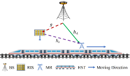
Figure 1: A RIS-assisted SISO downlink system for HST communications.

II-B Channel Model

We assume that all the links follow the Rician fading since line-of-sight (LoS) and non-line-of-sight (NLoS) components exist [25]. In time slot $t$, BS-RIS link $h_{\rm{d}}\left(t\right)$ can be expressed as

$$h_{\rm{d}}\left(t\right)=\sqrt{\frac{\kappa_{\rm{d}}}{\kappa_{\rm{d}}+1}}\bar{h}_{\rm{d}}\left(t\right)+\sqrt{\frac{1}{\kappa_{\rm{d}}+1}}\tilde{h}_{\rm{d}}\left(t\right),$$ (3)

where $\kappa_{\rm{d}}\geq 0$ is the Rician K-factor, $\bar{h}_{\rm{d}}\left(t\right)\in\mathbb{C}$ is the LoS component depending on BS-MR link and remains stable with each time slot, $\tilde{h}_{\rm{d}}\left(t\right)\in\mathbb{C}$ is the NLoS component. The LoS component of the channel between BS and MR can be given as [27] $\bar{h}_{\rm{d}}\left(t\right)=\sqrt{D_{\rm{d}}^{-\varepsilon_{\rm{d}}}\left(t\right)}e^{-j\theta_{\rm{d}}\left(t\right)}$, where $D_{\rm{d}}\left(t\right)$ denotes distance between BS and MR, as shown in Fig. 2, $\varepsilon_{\rm{d}}\left(t\right)$ denotes path-loss parameter, and $\theta_{\rm{d}}\left(t\right)$ denote phase. Similarly, the NLoS component can be written as $\tilde{h}_{\rm{d}}\left(t\right)=\sqrt{d_{\rm{NLoS,d}}^{-\varepsilon^{\prime}_{\rm{d}}}\left(t\right)}\tilde{h}_{\rm{NLoS}}^{\rm{d}}\left(t\right)$, where $d_{\rm{NLoS,d}}\left(t\right)$ is the distance between BS and MR for the NLoS case, $\varepsilon^{\prime}_{\rm{d}}$ is the path-loss parameter, $\tilde{h}_{\rm{NLoS}}^{\rm{d}}\left(t\right)\sim\mathcal{C}\mathcal{N}(0,1)$ denotes small-scale channel component.

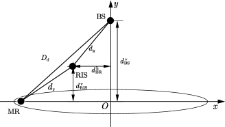
Figure 2: Top view of RIS-assisted HST communication system model.

For all $n\in\mathcal{N}$, in time slot $t$, $g_{n}\left(t\right)$ and $h_{\rm{r}}^{n}\left(t\right)$ can be given as

$$g_{n}\left(t\right)=\sqrt{\frac{\kappa_{\rm{g}}}{\kappa_{\rm{g}}+1}}\bar{h}_{\rm{g}}^{n}+\sqrt{\frac{1}{\kappa_{\rm{g}}+1}}\tilde{h}_{\rm{g}}^{n}\left(t\right),$$ (4)

$$h_{\rm{r}}^{n}\left(t\right)=\sqrt{\frac{\kappa_{\rm{r}}}{\kappa_{\rm{r}}+1}}\bar{h}_{\rm{r}}^{n}\left(t\right)+\sqrt{\frac{1}{\kappa_{\rm{r}}+1}}\tilde{h}_{\rm{r}}^{n}\left(t\right),$$ (5)

where $\kappa_{\rm{g}}\geq 0$ and $\kappa_{\rm{r}}\geq 0$ are the Rician K-factors, $\bar{h}_{\rm{g}}^{n}\in\mathbb{C}$ and $\bar{h}_{\rm{r}}^{n}\left(t\right)\in\mathbb{C}$ denote LoS components, and $\tilde{h}_{\rm{g}}^{n}\left(t\right)\in\mathbb{C}$ and $\tilde{h}_{\rm{r}}^{n}\left(t\right)\in\mathbb{C}$ denote NLoS components. Similar to BS-MR link, we have $\bar{h}_{\rm{g}}^{n}=\sqrt{\left(d_{\rm{g}}^{n}\right)^{-\varepsilon_{\rm{g}}}}e^{-j\theta_{\rm{g}}^{n}}$, $\bar{h}_{\rm{r}}^{n}\left(t\right)=\sqrt{\left(d_{\rm{r}}^{n}\left(t\right)\right)^{-\varepsilon_{\rm{r}}}}e^{-j\theta_{\rm{r}}^{n}\left(t\right)}$, where $d_{\rm{g}}^{n}$ and $d_{\rm{r}}^{n}\left(t\right)$ denote distance between BS and the $n$-th RIS and between the $n$-th RIS element and MR, as shown in Fig. 2, respectively. Moreover, $d_{\rm{BS}}^{\rm{v}}$ denotes vertical distance from BS to rail track, $d_{\rm{RIS}}^{\rm{v}}$ denotes vertical distance from RIS to rail track, and $d_{\rm{BR}}^{\rm{h}}$ denotes horizontal distance between BS and RIS. Parameters $\varepsilon_{\rm{g}}$ and $\varepsilon_{\rm{r}}$ are path-loss parameters, and $\theta_{\rm{g}}^{n}$ and $\theta_{\rm{r}}^{n}\left(t\right)$ are phase. Similarly, the NLoS component can be written as $\tilde{h}_{\rm{g}}^{n}\left(t\right)=\sqrt{\left(d_{\rm{NLoS,g}}^{n}\right)^{-\varepsilon^{\prime}_{\rm{g}}}}\tilde{h}_{\rm{NLoS,g}}^{n}\left(t\right)$, $\tilde{h}_{\rm{r}}^{n}\left(t\right)=\sqrt{\left(d_{\rm{NLoS,r}}^{n}\left(t\right)\right)^{-\varepsilon^{\prime}_{\rm{r}}}}\tilde{h}_{\rm{NLoS,r}}^{n}\left(t\right)$, where $d_{\rm{NLoS,g}}^{n}$, $d_{\rm{NLoS,r}}^{n}\left(t\right)$ denote distance between BS and the $n$-th RIS and between the $n$-th RIS and MR in the NLoS case, respectively. Parameters $\varepsilon^{\prime}_{\rm{g}}$, $\varepsilon^{\prime}_{\rm{r}}$ are the path-loss parameters in the NLoS case, and $\tilde{h}_{\rm{NLoS,g}}^{n}\left(t\right),\tilde{h}_{\rm{NLoS,r}}^{n}\left(t\right)\sim\mathcal{C}\mathcal{N}(0,1)$ denote the small-scale components.

III Coverage Probability Analysis and RIS Phase Optimization

In this section, we derive the expression of coverage probability for RIS-assisted HST communications. Then, we proposed an local search method to optimize the RIS phase.

III-A Coverage Probability

Coverage probability is defined as the probability that the effectively received SNR $\gamma\left(t\right)$ at MR is larger than a given SNR threshold $\gamma_{th}$, which can be given by

$$P_{\rm{cov}}\left(t\right)=\mathrm{Pr}\left(\gamma\left(t\right)\geqslant\gamma_{\rm{th}}\right)=1-\mathrm{Pr}\left(\gamma\left(t\right)<\gamma_{\rm{th}}\right).$$ (6)

Let $P_{\rm{out}}\left(t\right)$ denote $\mathrm{Pr}\left(\gamma\left(t\right)<\gamma_{\rm{th}}\right)$, and it is given by

$$\begin{array}[]{l}P_{\rm{out}}\left(t\right)\\ =\mathrm{Pr}\left(\frac{P\left|h_{\rm{d}}\left(t\right)+\sum_{n=1}^{N}{h^{r}_{{\rm{n}}}\left(t\right)e^{j\theta_{n}\left(t\right)}g_{n}}\left(t\right)\right|^{2}}{\sigma^{2}}<\gamma_{\rm{th}}\right)\\ =\mathrm{Pr}\left(\left|h_{\rm{d}}\left(t\right)+\sum_{n=1}^{N}{h^{n}_{{\rm{r}}}\left(t\right)e^{j\theta_{n}\left(t\right)}h^{n}_{{\rm{g}}}}\left(t\right)\right|^{2}<\frac{\gamma_{\rm{th}}}{\bar{\gamma}}\right)\\ =\mathrm{Pr}\left(\left|h\left(t\right)\right|^{2}<\frac{\gamma_{\rm{th}}}{\bar{\gamma}}\right).\end{array}$$ (7)

where $\bar{\gamma}=\frac{P}{\sigma^{2}}$ denotes the average transmission SNR.

The type of probability distribution of $h\left(t\right)$ is given by Theorem 1.

Theorem 1.

The equivalent channel $h\left(t\right)$ between BS and MR, follows complex-valued Gaussian distribution with mean $\mu_{h}\left(t\right)$ and variance $\sigma_{h}^{2}\left(t\right)$, namely, $h\left(t\right)\sim\mathcal{C}\mathcal{N}\left(\mu_{h}\left(t\right),\sigma_{h}^{2}\left(t\right)\right)$, and we have

$$\mu_{h}\left(t\right) =\rho_{\rm{d}}\sqrt{D_{\rm{d}}^{-\varepsilon_{\rm{d}}}\left(t\right)}e^{-j\theta_{\rm{d}}\left(t\right)}$$ (8)

$$+\sum_{n=1}^{N}\rho_{\rm{r}}\rho_{\rm{g}}\sqrt{\left(d_{\rm{r}}^{n}\left(t\right)\right)^{-\varepsilon_{\rm{r}}}}\sqrt{\left(d_{\rm{g}}^{n}\right)^{-\varepsilon_{\rm{g}}}}$$

$$\times e^{j\left(\theta_{n}\left(t\right)-\theta_{\rm{r}}^{n}\left(t\right)-\theta_{\rm{g}}^{n}\right)},$$

$$\sigma_{h}^{2}\left(t\right) =\varrho_{\rm{d}}^{2}d_{\rm{NLoS,d}}^{-\varepsilon^{\prime}_{\rm{d}}}\left(t\right)$$ (9)

$$+\sum_{n=1}^{N}\varrho_{\rm{r}}^{2}\varrho_{\rm{g}}^{2}\left(d_{\rm{NLoS,r}}^{n}\left(t\right)\right)^{-\varepsilon^{\prime}_{\rm{r}}}\left(d_{\rm{NLoS,g}}^{n}\right)^{-\varepsilon^{\prime}_{\rm{g}}},$$

where $\rho_{\rm{d}}=\sqrt{\frac{\kappa_{{\rm{d}}}}{\kappa_{{\rm{d}}}+1}}$, $\varrho_{{\rm{d}}}=\sqrt{\frac{1}{\kappa_{\rm{d}}+1}}$, $\rho_{\rm{g}}=\sqrt{\frac{\kappa_{{\rm{g}}}}{\kappa_{{\rm{g}}}+1}}$, $\varrho_{{\rm{g}}}=\sqrt{\frac{1}{\kappa_{{\rm{g}}}+1}}$, $\rho_{\rm{r}}=\sqrt{\frac{\kappa_{\rm{r}}}{\kappa_{\rm{r}}+1}}$, and $\varrho_{{\rm{r}}}=\sqrt{\frac{1}{\kappa_{\rm{r}}+1}}$.

Proof.

See Appendix A. ∎

According to Theorem 1, the coverage probability can be derived as in Theorem 2.

Theorem 2.

$P_{\rm{out}}\left(t\right)$ follows a non-central chi-square distribution, i.e., $\chi^{2}\left(\nu,\zeta\left(t\right)\right)$, with the degree freedom $\nu=1$ , and the non-centrality parameter $\zeta\left(t\right)=\frac{\mu_{h}^{2}\left(t\right)}{\sigma_{h}^{2}\left(t\right)}$, where

$$\begin{array}[]{l}\left|\mu_{h}\left(t\right)\right|^{2}=\left|\rho_{\rm{d}}\sqrt{D_{\rm{d}}^{-\varepsilon_{\rm{d}}}\left(t\right)}e^{-j\theta_{\rm{d}}\left(t\right)}\right.\\ \left.+\sum_{n=1}^{N}\rho_{\rm{r}}\rho_{\rm{g}}\sqrt{\left(d_{\rm{r}}^{n}\left(t\right)\right)^{-\varepsilon_{\rm{r}}}}\sqrt{\left(d_{\rm{g}}^{n}\right)^{-\varepsilon_{\rm{g}}}}e^{j\left(\theta_{n}\left({t}\right)-\theta_{\rm{r}}^{n}\left({t}\right)-\theta_{\rm{g}}^{n}\right)}\right|^{2}.\end{array}$$ (10)

With the corresponding cumulative distribution function (CDF), $P_{\rm{out}}\left(t\right)$ is given by

$$P_{\rm{out}}\left(t\right)=1-Q_{\frac{1}{2}}\left(\sqrt{\zeta\left(t\right)},\sqrt{\gamma_{0}\left(t\right)}\right),$$ (11)

where $\gamma_{0}=\frac{\gamma_{th}}{\bar{\gamma}\sigma_{h}^{2}\left(t\right)}$, and $Q_{m}\left(a,b\right)$ is the Marcum Q-function defined in [28]. Thus, the coverage probability can be expressed as

$$P_{\rm{cov}}=1-P_{\rm{out}}=Q_{\frac{1}{2}}\left(\sqrt{\zeta\left(t\right)},\sqrt{\gamma_{0}\left(t\right)}\right).$$ (12)

Proof.

See Appendix B. ∎

III-B RIS Phase Optimization

The set of discrete phase $\varTheta$ contains a series of discrete variables, and the range available for each phase depends on RIS quantization bits. Considering the complexity and validity, we exploit the local search method as shown in Algorithm 1 to optimize the phase. Specifically, keeping the other $N-1$ phase values fixed, for each element $\theta_{n}\left(t\right)$, we traverse all possible values and choose the optimal one. Then, use this optimal solution $\theta_{n}^{\ast}\left(t\right)$ as the new value of $\theta_{n}\left(t\right)$ for the optimization of another phase, until all phases in the set $\varTheta$ are fully optimized.

Algorithm 1 Local Search for Discrete phase

0:  the toal time $T$ slots, the number of quantization bits $b$

0:  $\theta_{n}^{\ast}\left(t\right),~{}\forall n\in\mathcal{N}$

1:  for $t=1:T$ do

2:     for $n=1:N$ do

3:        Assign all possible values to $\theta_{n}\left(t\right)$, and select the value maximizing the coverage probability $P_{\rm{cov}}\left(t\right)$ denoted as $\theta_{n}^{\ast}\left(t\right)$;

4:        $\theta_{n}\left(t\right)=\theta_{n}^{\ast}\left(t\right)$;

5:     end for

6:  end for

IV Numerical Analysis

In this section, we analyze coverage probability of RIS-assisted HST communications. Simulation results are provided to validate system performance in terms of coverage probability. For comparison, the scheme without using RIS is considered, which does not use RIS for signal reflection and MR can only receive signals through BS-MR channels. The simulation parameters are set as listed in Table I.

TABLE I: Simulation Parameters

Parameter	Symbol	Value
Speed of HST	$v$	$360$ km/h
Height of BS	$H_{\rm{BS}}$	$10$ m
Height of RIS	$H_{\rm{RIS}}$	$2$ m
Height of MR	$H_{\rm{MR}}$	$2.5$ m
Bandwidth	$B$	$20$ MHz
Noise power	$\sigma^{2}$	$-174$ dBm/Hz $+10\log_{10}B+10$ dB
Carrier frequency	$f$	$2.35$ GHz
Rician factor	$\kappa_{\left({\rm{d,r,g}}\right)}$	$10$ dB

Fig. 3 illustrates coverage probability $P_{\rm{cov}}$ against transmission power under two schemes and varying numbers of RIS elements. It can be observed that coverage probabilities under these two schemes increase with increasing of the transmission power. Coverage probability of using RIS outperforms the case without RIS. It can be further observed that as the number of RIS elements $N$ increases, $P_{\rm{cov}}$ increases. This is because more RIS elements in the system result that more signal paths and energy can be reflected to enhance the signal quality at MR.

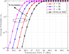
Figure 3: Coverage probability vs. transmission power.

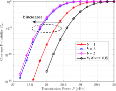
Figure 4: Coverage probability vs. transmission power.

Fig. 4 shows coverage probability $P_{\rm{cov}}$ against transmission power under different schemes and varying numbers of RIS quantization bits. It can be observed that $P_{\rm{cov}}$ increases with increasing number of RIS quantization bits $b$. It can be observed that coverage probability of $b=1$ is significantly lower than $b=3$ and $b=5$, which means that coverage probability is significantly improved when $b>1$. This is because phase resolution increases with increasing $b$, which results that the received power at MR is enhanced. It can be further observed that the narrow coverage probability gap exists between $b=3$ and $b=5$, which indicates that coverage probability may remain unchanged with further increasing $b$.

Fig. 5 illustrates coverage probability $P_{\rm{cov}}$ versus the SNR threshold $\gamma_{th}$ under different numbers of RIS elements. It can be observed that coverage probabilities under these two schemes decrease with increasing transmission power. Obviously, improving SNR threshold requirement means more outage events and lower coverage probability. When $N$ increases, channel gain of $h\left(t\right)$ increases, which result that the received power at MR is enhanced and the coverage probability is thus improved.

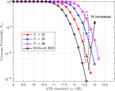
Figure 5: Coverage probability vs. SNR threshold.

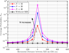
Figure 6: Coverage probability vs. horizontal distance between BS and RIS.

Fig. 6 shows impact of horizontal distances $d_{\rm{BR}}^{\rm{h}}$ between RIS and BS, as shown in Fig. 2, on coverage probability. It is observed that the coverage probability of the cases using RIS firstly increases and then decreases, while the case with using RIS dose not change with location. It is found that when horizontal distance $d_{\rm{BR}}^{\rm{h}}$ is equal to $-600$ m or $600$ m, i.e., at the edge of the investigated area, the coverage probability is lowest. While horizontal distance $d_{\rm{BR}}^{\rm{h}}$ is equal to $0$, which is the center of the long axis of BS elliptical coverage area, the coverage probability is high. This is owing to the fact that when RIS moves towards the center of the area, path loss of reflection link changes accordingly, which leads to an enhancement of the reflected signal and the benefits of RIS are fully utilized. This show that system performance is sensitive to placement of RIS.

V Conclusion

In this paper, we investigate wireless coverage probability analysis of downlink SISO RIS-assisted HST communication system. An closed-form expression of the coverage probability is derived. We have analyzed the impact of different system parameters on coverage probability including transmission power, SNR threshold, and horizontal distance between BS and RIS. Numerical results have demonstrated that better coverage performance can be achieved by using well RIS. The results in this paper can serve as a guidance for RIS-assisted HST communication coverage analysis.

Appendix A

Substituting (3), (4) and (5) into $h\left(t\right)$, we have

$$h\left(t\right)=\rho_{\rm{d}}\bar{h}_{\rm{d}}\left(t\right)+\varrho_{{\rm{d}}}\tilde{h}_{\rm{d}}\left(t\right)+\sum_{n=1}^{N}{\rho_{\rm{r}}\rho_{\rm{g}}\bar{h}^{n}_{{\rm{r}}}\left(t\right)e^{j\theta_{n}\left(t\right)}\bar{h}^{n}_{{\rm{g}}}}$$ (13)

$$+\sum_{n=1}^{N}{\rho_{\rm{r}}\varrho_{{\rm{g}}}\bar{h}^{n}_{{\rm{r}}}\left(t\right)e^{j\theta_{n}\left(t\right)}\tilde{h}^{n}_{{\rm{g}}}}\left(t\right)+\sum_{n=1}^{N}{\varrho_{\rm{r}}\rho_{{\rm{g}}}\tilde{h}^{n}_{{\rm{r}}}\left(t\right)e^{j\theta_{n}\left(t\right)}\bar{h}^{n}_{{\rm{g}}}}$$

$$+\sum_{n=1}^{N}{\varrho_{\rm{r}}\varrho_{{\rm{g}}}\tilde{h}^{n}_{{\rm{r}}}\left(t\right)e^{j\theta_{n}\left(t\right)}\tilde{h}^{n}_{{\rm{g}}}}\left(t\right),$$

where $\rho_{\rm{d}}=\sqrt{\frac{\kappa_{{\rm{d}}}}{\kappa_{{\rm{d}}}+1}}$, $\varrho_{{\rm{d}}}=\sqrt{\frac{1}{\kappa_{\rm{d}}+1}}$, $\rho_{\rm{g}}=\sqrt{\frac{\kappa_{{\rm{g}}}}{\kappa_{{\rm{g}}}+1}}$, $\varrho_{{\rm{g}}}=\sqrt{\frac{1}{\kappa_{{\rm{g}}}+1}}$, $\rho_{\rm{r}}=\sqrt{\frac{\kappa_{\rm{r}}}{\kappa_{\rm{r}}+1}}$, and $\varrho_{{\rm{r}}}=\sqrt{\frac{1}{\kappa_{\rm{r}}+1}}$. Note that, the LoS components of BS-MR link, RIS-MR link and BS-RIS link depend on the corresponding link distances. For a given location, the components $\rho_{\rm{d}}\bar{h}_{\rm{d}}\left(t\right)$ and $\sum_{n=1}^{N}{\rho_{\rm{r}}\rho_{\rm{g}}\bar{h}^{n}_{{\rm{r}}}\left(t\right)e^{j\theta_{n}\left(t\right)}\bar{h}^{n}_{{\rm{g}}}}$ of (13) turn to be deterministic. Since the NLoS component $\tilde{h}_{\rm{d}}\left(t\right)$ follows complex Gaussian distribution with zero mean and variance $d_{\rm{NLoS,d}}^{-\varepsilon^{\prime}_{\rm{d}}}\left(t\right)$, $\tilde{h}_{\rm{r}}\left(t\right)$ and $\tilde{h}_{\rm{g}}\left(t\right)$ follow complex Gaussian distribution with zero mean and variance $\left(d_{\rm{NLoS,r}}^{n}\left(t\right)\right)^{-\varepsilon^{\prime}_{\rm{r}}}$, $\left(d_{\rm{NLoS,g}}^{n}\right)^{-\varepsilon^{\prime}_{\rm{g}}}$, respectively, and the parts $\varrho_{{\rm{d}}}\tilde{h}_{\rm{d}}\left(t\right)$, $\sum_{n=1}^{N}{\rho_{\rm{r}}\varrho_{{\rm{g}}}\bar{h}^{n}_{{\rm{r}}}\left(t\right)e^{j\theta_{n}\left(t\right)}\tilde{h}^{n}_{{\rm{g}}}}\left(t\right)$, $\sum_{n=1}^{N}{\varrho_{\rm{r}}\rho_{{\rm{g}}}\tilde{h}^{n}_{{\rm{r}}}\left(t\right)e^{j\theta_{n}\left(t\right)}\bar{h}^{n}_{{\rm{g}}}}$ and $\sum_{n=1}^{N}{\varrho_{\rm{r}}\varrho_{{\rm{g}}}\tilde{h}^{n}_{{\rm{r}}}\left(t\right)e^{j\theta_{n}\left(t\right)}\tilde{h}^{n}_{{\rm{g}}}}\left(t\right)$ of (13) also follow a Gaussian distribution.

The expectation of $h\left(t\right)$ can be written by

$$\mu_{h}\left(t\right)\triangleq\mathbb{E}\left\{h\left(t\right)\right\}$$ (14)

$$=\rho_{\rm{d}}\bar{h}_{\rm{d}}\left(t\right)+\sum_{n=1}^{N}{\rho_{\rm{r}}\rho_{\rm{g}}\bar{h}^{n}_{{\rm{r}}}\left(t\right)e^{j\theta_{n}\left(t\right)}\bar{h}^{n}_{{\rm{g}}}}$$

$$=\rho_{\rm{d}}\sqrt{D_{\rm{d}}^{-\varepsilon_{\rm{d}}}\left(t\right)}e^{-j\theta^{\rm{d}}\left(t\right)}$$

$$+\sum_{n=1}^{N}\rho_{\rm{r}}\rho_{\rm{g}}\sqrt{\left(d_{\rm{r}}^{n}\left(t\right)\right)^{-\varepsilon_{\rm{r}}}}\sqrt{\left(d_{\rm{g}}^{n}\right)^{-\varepsilon_{\rm{g}}}}e^{j\left(\theta_{n}\left(t\right)-\theta_{\rm{r}}^{n}\left(t\right)-\theta_{\rm{g}}^{n}\right)}.$$

The variance of $h\left(t\right)$ is derived as

$$\sigma_{h}^{2}\left(t\right)\triangleq\rm{var}\left\{h\left(t\right)\right\}$$ (15)

$$=\varrho_{{\rm{d}}}^{2}\rm{var}\left\{\tilde{h}_{\rm{d}}\left(t\right)\right\}+\varrho_{\rm{r}}^{2}\varrho_{{\rm{g}}}^{2}\rm{var}\left\{\sum_{n=1}^{N}{\tilde{h}^{n}_{{\rm{r}}}\left(t\right)e^{j\theta_{n}\left(t\right)}\tilde{h}^{n}_{{\rm{g}}}}\left(t\right)\right\}$$

$$=\varrho_{\rm{d}}^{2}d_{\rm{NLoS,d}}^{-\varepsilon^{\prime}_{\rm{d}}}\left(t\right)+\sum_{n=1}^{N}\varrho_{\rm{r}}^{2}\varrho_{\rm{g}}^{2}\left(d_{\rm{NLoS,r}}^{n}\left(t\right)\right)^{-\varepsilon^{\prime}_{\rm{r}}}\left(d_{\rm{NLoS,g}}^{n}\right)^{-\varepsilon^{\prime}_{\rm{g}}}.$$

Therefore, $h\left(t\right)$ is proved to follow a complex-valued Gaussian distribution, $h\left(t\right)\sim\mathcal{C}\mathcal{N}\left(\mu_{h}\left(t\right),\sigma_{h}^{2}\left(t\right)\right)$. This completes the proof.

Appendix B

Due to the Gaussian channel proved above, $h\left(t\right)\sim\mathcal{C}\mathcal{N}\left(\mu_{h}\left(t\right),\sigma_{h}^{2}\left(t\right)\right)$. Therefore, $\frac{\left|h\left(t\right)\right|^{2}}{\sigma_{h}^{2}\left(t\right)}$ follows the non-central chi-squared distribution, i.e., $\chi^{2}(\nu,\zeta\left(t\right))$, with the degrees of freedom $\nu=1$, and the non-centrality parameter is in (16).

$$\zeta\left(t\right)=\frac{\left|\mu_{h}\left(t\right)\right|^{2}}{\sigma_{h}^{2}\left(t\right)}=\frac{\left|\rho_{\rm{d}}\sqrt{D_{\rm{d}}^{-\varepsilon_{\rm{d}}}\left(t\right)}e^{-j\theta^{\rm{d}}\left(t\right)}+\sum_{n=1}^{N}\rho_{\rm{r}}\rho_{\rm{g}}\sqrt{\left(d_{\rm{r}}^{n}\left(t\right)\right)^{-\varepsilon_{\rm{r}}}}\sqrt{\left(d_{\rm{g}}^{n}\right)^{-\varepsilon_{\rm{g}}}}e^{j\left(\theta_{n}\left(t\right)-\theta_{\rm{r}}^{n}\left(t\right)-\theta_{\rm{g}}^{n}\right)}\right|^{2}}{\varrho_{\rm{d}}^{2}d_{\rm{NLoS,d}}^{-\varepsilon^{\prime}_{\rm{d}}}\left(t\right)+\sum_{n=1}^{N}\varrho_{\rm{r}}^{2}\varrho_{\rm{g}}^{2}\left(d_{\rm{NLoS,r}}^{n}\left(t\right)\right)^{-\varepsilon^{\prime}_{\rm{r}}}\left(d_{\rm{NLoS,g}}^{n}\right)^{-\varepsilon^{\prime}_{\rm{g}}}}.$$ (16)

With the corresponding CDF of $\chi^{2}(\nu,\zeta\left(t\right))$, $P_{\rm{out}}\left(t\right)$ defined in (6) is given by

$$P_{\rm{out}}\left(t\right)=1-Q_{\frac{1}{2}}\left(\sqrt{\zeta\left(t\right)},\sqrt{\gamma_{0}\left(t\right)}\right),$$ (17)

where $\gamma_{0}=\frac{\gamma_{th}}{\bar{\gamma}\sigma_{h}^{2}\left(t\right)}$, and $Q_{m}\left(a,b\right)$ is the Marcum Q-function defined in [28]. As a result, the coverage probability defined in (6) can be rewrite as

$$P_{\rm{cov}}=Q_{\frac{1}{2}}\left(\sqrt{\zeta\left(t\right)},\sqrt{\gamma_{0}\left(t\right)}\right).$$ (18)

This completes the proof.

References

- [1] J. Zhang, H. Liu, Q. Wu, Y. Jin, Y. Chen, B. Ai, S. Jin and T. J. Cui, “RIS-aided next-generation high-speed train communications: challenges, solutions, and future directions,” IEEE Wireless Communications, vol. 28, no. 6, pp. 145–151, Dec. 2021.
- [2] R. He, B. Ai, G. Wang, M. Yang, C. Huang and Z. Zhong, “Wireless channel sparsity: measurement, analysis, and exploitation in estimation,” IEEE Wireless Communications, vol. 28, no. 4, pp. 113–119, Aug. 2021.
- [3] C. Huang, R. He, B. Ai, A. F. Molisch, B. Kiong Lau, K. Haneda, B. Liu, C.-X. Wang, M. Yang, C. Oestges and Z. Zhong, “Artificial intelligence enabled radio propagation for communications—part I: channel characterization and antenna-channel optimization,” IEEE Transactions on Antennas and Propagation, early access, doi: 10.1109/TAP.2022.3149663.
- [4] C. Huang, R. He, B. Ai, A. F. Molisch, B. Kiong Lau, K. Haneda, B. Liu, C.-X. Wang, M. Yang, C. Oestges and Z. Zhong, “Artificial intelligence enabled radio propagation for communications—part II: scenario identification and channel modeling,” IEEE Transactions on Antennas and Propagation, early access, doi: 10.1109/TAP.2022.3149665.
- [5] M. A. ElMossallamy, H. Zhang, L. Song, K. G. Seddik, Z. Han and G. Y. Li, “Reconfigurable intelligent surfaces for wireless communications: principles, challenges, and opportunities,” IEEE Transactions on Cognitive Communications and Networking, vol. 6, no. 3, pp. 990–1002, Sep. 2020.
- [6] G. Sun, R. He, B. Ai, Z. Ma, P. Li, Y. Niu, W. J. Ding, D. Fei and Z. Zhong, “A 3D wideband channel model for RIS-assisted MIMO communications,” IEEE Transactions on Vehicular Technology, early access, doi: 10.1109/TVT.2022.3175223.
- [7] R. Liu, Q. Wu, M. Di Renzo and Y. Yuan, “A path to smart radio environments: an industrial viewpoint on reconfigurable intelligent surfaces,” IEEE IEEE Wireless Communications, vol. 29, no. 1, pp. 202–208, Feb. 2022.
- [8] L. Yan, X. Fang, L. Hao and Y. Fang, “Safety-oriented resource allocation for space-ground integrated cloud networks of high-speed railways,” IEEE Journal on Selected Areas in Communications, vol. 38, no. 12, pp. 2747–2759, Dec. 2020.
- [9] X. Liu and D. Qiao, “Elliptical cell based beamforming design with an improved -fairness power allocation for HSR communication systems,” China Communications, early access, doi: 10.23919/JCC.2021.00.003.
- [10] X. Liu and D. Qiao, “Design and coverage analysis of elliptical cell based beamforming for HSR communication systems,” in Proc. IEEE International Conference on Communications, Shanghai, China, May 2019, pp. 1–6.
- [11] S.-H. Lin, Y. Xu, and J.-Y. Wang, “Coverage analysis and optimization for high-speed railway communication systems with arrow-strip-shaped cells,” IEEE Transactions on Vehicular Technology, vol. 69, no. 10, pp. 11544–11556, Oct. 2020.
- [12] S.-H. Lin, Y. Xu, and J.-Y. Wang, “Cell coverage analysis for high-speed railway communication systems with hard handoff,” in Proc. International Conference on Wireless Communications and Signal Processing, Xi’an, China, Oct. 2019, pp. 1–6.
- [13] J. -Y. Zhang, Z. -H. Tan and X. -X. Yu, “Coverage efficiency of radio-over-fiber network for high-speed railways,” in Proc. International Conference on Wireless Communications Networking and Mobile Computing, Chengdu, China, Sep. 2010, pp. 1–4.
- [14] S. Fathi-Kazerooni, Y. Kaymak, R. Rojas-Cessa, J. Feng, N. Ansari, M. Zhou and T. Zhang, “Optimal positioning of ground base stations in free-space optical communications for high-speed trains,” IEEE Transactions on Intelligent Transportation Systems, vol. 19, no. 6, pp. 1940–11949, Jun. 2018.
- [15] H. S. Khallaf and M. Uysal, “UAV-based FSO communications for high speed train backhauling,” in Proc. IEEE Wireless Communications and Networking Conference, Marrakesh, Morocco, Apr. 2019, pp. 1–6.
- [16] W. Zeng, J. Zhang, K. P. Peppas, B. Ar and Z. Zhong, “UAV-aided wireless information and power transmission for high-speed train communications,” in Proc. International Conference on Intelligent Transportation Systems, Maui, HI, USA, Nov. 2018, pp. 3409–3414.
- [17] S. -H. Lin, Y. Xu, L. Wang and J. -Y. Wang, “Coverage analysis and chance-constrained optimization for HSR communications with carrier aggregation,” IEEE Transactions on Intelligent Transportation Systems, early access, doi: 10.1109/TITS.2021.3137030.
- [18] M. Gao, B. Ai, Y. Niu, Z. Han and Z. Zhong, “IRS-assisted high-speed train communications: outage probability minimization with statistical CSI,” in Proc. IEEE International Conference on Communications, Montreal, QC, Canada, Jun. 2021, pp. 1–6.
- [19] T. Li, H. Tong, Y. Xu, X. Su and G. Qiao, “Double-IRSs aided massive MIMO channel estimation and spectrum efficiency maximization for high-speed railway communications,” IEEE Transactions on Vehicular Technology, early access, doi: 10.1109/TVT.2022.3174420.
- [20] J. Xu and B. Ai, “When mmWave high-speed railway networks meet reconfigurable intelligent surface: a deep reinforcement learning method,” IEEE Wireless Communications Letters, vol. 11, no. 3, pp. 533–537, Mar. 2022.
- [21] P. Agheli, H. Beyranvand and M. Javad Emadi, “High-speed trains access connectivity through RIS-assisted FSO communications,” Oct. 2021, arXiv:2110.12804. [Online]. Available: https://doi.org/10.48550/arXiv.2110.12804
- [22] Z. Ma, Y. Wu, M. Xiao, G. Liu and Z. Zhang, “Interference suppression for railway wireless communication systems: a reconfigurable intelligent surface approach,” IEEE Transactions on Vehicular Technology, vol. 70, no. 11, pp. 11593–11603, Nov. 2021.
- [23] T. J. Cui, M. Q. Qi, X. Wan, J. Zhao, and Q. Cheng, “Coding metamaterials, digital metamaterials and programmable metamaterials,” Light Sci Appl , vol. 3, no. 10, p. e218, Oct. 2014.
- [24] E. Basar, M. Di Renzo, J. De Rosny, M. Debbah, M. S. Alouini, and R. Zhang, “Wireless communications through reconfigurable intelligent surfaces,” IEEE Access, vol. 7, pp. 116753–116773, 2019.
- [25] Y. Cai, M.-M. Zhao, K. Xu, and R. Zhang, “Intelligent reflecting surface aided full-duplex communication: passive beamforming and deployment design,” IEEE Transactions on Wireless Communications, vol. 21, no. 1, pp. 383–397, Jan. 2022.
- [26] Y. Zhang and L. Dai, “A closed-form approximation for uplink average ergodic sum capacity of large-scale multi-user distributed antenna systems,” IEEE Transactions on Vehicular Technology, vol. 68, no. 2, pp. 1745–1756, Feb. 2019.
- [27] A. Goldsmith, Wireless Communications, Cambridge Press, 2005.
- [28] V. M. Kapinas, S. K. Mihos, and G. K. Karagiannidis, “On the monotonicity of the generalized Marcum and Nuttall -functions,” IEEE Transactions on Information Theory, vol. 55, no. 8, pp. 3701–3710, Aug. 2009.