A Stable Weighted Residual Finite Element Formulation for the Simulation of Linear Moving Conductor Problems

Abstract

The finite element method is one of the widely employed numerical techniques in electrical engineering for the study of electric and magnetic fields. When applied to the moving conductor problems, the finite element method is known to have numerical oscillations in the solution. To resolve this, the upwinding techniques, which are developed for the transport equation are borrowed and directly employed for the magnetic induction equation. In this work, an alternative weighted residual formulation is explored for the simulation of the linear moving conductor problems. The formulation is parameter-free and the stability of the formulation is analytically studied for the 1D version of the moving conductor problem. Then the rate of convergence and the accuracy are illustrated with the help of several test cases in 1D as well as 2D. Subsequently, the stability of the formulation is demonstrated with a 3D moving conductor simulation.

I Introduction

The finite element method is a widely used numerical technique for the design and analysis of electrical machines and instruments. The Galerkin finite element (GFE) formulation is known to produce highly accurate solutions for electrostatic and magnetostatic simulations. However, for the simulation of linear moving conductors, such as linear induction motor, magnetic brakes, electromagnetic flowmeter etc., the numerical stability problem occurs at high velocities [1, 2, 3].

The numerical stability problem at high velocities is also common to the transport equation of fluid dynamics [4]. The numerical oscillation in the simulation of transport equation is well studied over several decades [5, 6]. It is observed from the finite difference formulation that the stability is restored, when the central difference of the first order term is reinforced/replaced with the one-sided difference along the flow direction [7, 8]. Following this observation, the common technique in finite element method is to upwind the weight function along the flow direction, so to make the first order term more one-sided [9, 10].

These upwinding techniques are borrowed from the transport equation and directly employed for the moving conductor problems [11, 12, 13, 14, 15, 16, 17]. Even though the upwinding techniques solve the numerical instability problem, there are other issues associated with the application of upwinding schemes, such as, crosswind diffusion and erroneous solution at the transverse boundary [10, 18, 19]. These errors were first observed for the transport equation and several remedies have been suggested, with partial success [20, 21]. The error at the transverse boundary observed for the moving conductor problems as well; and a solution is suggested in a recent literature [22, 23].

Given these, in this work, a weighted residual finite element formulation is suggested, by eliminating the first order derivatives in the governing equation of the moving conductor problem, in a way it is consistent. Thus, the term which introduces numerical instability is eliminated and numerical stability can be achieved. It can also be noted that such a formulation does not require a stabilization parameter - $\tau$, like the upwinding schemes. Thus, this formulation remains parameter-free.

Firstly, stability analysis is performed for the weighted residual formulation in 1D. Then the numerical exercises are carried out for 1D, as well as, 2D problems to check the accuracy and the convergence. In addition to this, a test case involving the magnetic material $\mu_{r}>1$ is simulated in 2D as well as in 3D, to verify the accuracy of the formulation with multiple materials. In the next section the analysis for the 1D problem is discussed.

II Analysis on the 1D moving conductor problem

The 1D version of the moving conductor problem is derived in [3] and it can be described as follows. In this, the source magnetic field is applied perpendicular to the plane of the paper ($x$-direction). The conductor of an infinite dimension, is moving along the horizontal $z$-axis with velocity $u_{z}$, permiability $\mu$ and conductivity $\sigma$. The reaction magnetic field $b_{x}$ is arising out of the motion and its vector potential is $A_{y}$. The governing equation for this problem can be written as,

$$-\dfrac{d^{2}A_{y}}{dz^{2}}+\mu\sigma u_{z}\dfrac{dA_{y}}{dz}=\mu\sigma u_{z}B_{x}$$ (1)

In this, the first derivative term can be eliminated from the governing equation, by writing the advective-first order term as $b_{x}=-{dA_{y}}/{dz}$. The equation (1) becomes,

$$-\dfrac{d^{2}A_{y}}{dz^{2}}-\mu\sigma u_{z}b_{x}=\mu\sigma u_{z}B_{x}$$ (2)

The Galerkin finite element formulation of (2) is written below with $N$ as weight (shape) function and the integration-by-parts is applied to the second-derivative diffusion term. In this, $A_{y}$, $b_{x}$ and the weight function $N$ belong to $H^{1}$ function space.

$$\int_{\Omega}\dfrac{dN}{dz}\dfrac{dA_{y}}{dz}~{}d\Omega-\mu\sigma u_{z}\int_{\Omega}Nb_{x}~{}d\Omega=\mu\sigma u_{z}\int_{\Omega}NB_{x}~{}d\Omega$$ (3)

Now the first derivative term is replaced with $b_{x}$ and it becomes a new unknown along with $A_{y}$. Therefore, we need a second equation to solve this system. The second equation is written below with the weight function of $dN/dz$, so as to eliminate the numerically unstable $N(dA_{y}/dz)$ term.

$$\int_{\Omega}\dfrac{dN}{dz}\dfrac{db_{x}}{dz}~{}d\Omega+\mu\sigma u_{z}\int_{\Omega}\dfrac{dN}{dz}\dfrac{dA_{y}}{dz}~{}d\Omega~{}\dots$$

$$=\mu\sigma u_{z}\int_{\Omega}\dfrac{dN}{dz}B_{x}~{}d\Omega$$ (4)

In this, the second derivative term $-{d^{2}A_{y}}/{dz^{2}}$ of (1) is replaced with ${db_{x}}/{dz}$. Equations (3) and (II) together can form a stable weighted formulation without any upwinding. In the next subsection, the stability analysis is carried out for (3) and (II).

II-A Stability analysis for the 1D weighted residual formulation

It can be readily noted that the governing equation of the 1D moving conductor problem (1) is same as that of the transport equation. However, in moving conductor problems, the boundary conditions on the magnetic vector potential $\bf{A}$ are not hard-imposed. The boundary conditions are always ‘${\bf A}=0$’ very far from the source magnetic field $\bf{B^{a}}$ or natural boundary conditions are chosen, if the problem permits [3]. Under this circumstance, the $Z$-transform based $pole$, $zero$ analysis is a good indicator for the numerical stability [3, 24] in moving conductor problems. Therefore, the same is employed here.

The difference equation form of the finite element equation (3), with linear elements, at the $n^{th}$ node can be written as,

$$-A_{y[n-1]}+2A_{y[n]}-A_{y[n+1]}-\dfrac{Pe}{3}(b_{x[n-1]}~{}\dots$$

$$+4b_{x[n]}+b_{x[n+1]})=\dfrac{Pe}{3}(B_{x[n-1]}+4B_{x[n]}+B_{x[n+1]})$$ (5)

and similarly the difference equation form of the finite element equation (II), with linear elements, at the $n^{th}$ node can be written as,

$$-b_{x[n-1]}+2b_{x[n]}-b_{x[n+1]}+2Pe(-A_{y[n-1]}~{}\dots$$

$$+2A_{y[n]}-A_{y[n+1]})=Pe(B_{x[n-1]}-B_{x[n+1]})$$ (6)

where $Pe$ is the Peclet number and it is defined as $Pe=\mu\sigma u_{z}\Delta z/2$. The Peclet number indicates the relative strength of advection over the diffusion in the difference equation. Taking $Z$-transform of the difference equations (II-A) and (II-A),

$$-A_{y}(Z^{2}-2Z+1)-\dfrac{Pe}{3}b_{x}(Z^{2}+4Z+1)~{}\dots$$

$$=\dfrac{Pe}{3}B_{x}(Z^{2}+4Z+1)$$ (7)

$$b_{x}(Z^{2}-2Z+1)+2PeA_{y}(Z^{2}-2Z+1)=PeB_{x}(Z^{2}-1)$$ (8)

Now, substituting the expression for $b_{x}$ from (II-A), in (8) and then approximating for $Pe>>1$, the final transfer function between $A_{y}$ and $B_{x}$ can be written as,

$$\dfrac{A_{y}}{B_{x}}\approx\dfrac{Z^{2}-1}{2(Z^{2}-2Z+1)}$$ (9)

The poles of the transfer function (9) are $Z=1,1$ and they are positive; indicating a stable formulation. In other words, the roots of the difference equations are positive for $Pe>>1$, resulting in a non-oscillatory system for the moving conductor problems. In the next subsection, the simulation results from 1D moving conductor problem are presented.

II-B Simulation results from 1D moving conductor problem

The finite element simulation of (1) is carried out, using the Galerkin formulation and the weighted residual formulation, which is described by equations (3) and (II). The simulation domain spans $0\leq z\leq 1$ and the input magnetic field $B_{x}=B,for~{}0.4\leq z\leq 0.6$. The simulations are carried out for different set of parameters and the results are observed to be accurate and stable. The sample simulation results for $Pe=4$ and $Pe=400$ are presented in Fig. 1. The figure 1 shows the reaction magnetic field $b_{x}=-dA_{y}/dz$ obtained from the i) proposed weighted residual formulation, ii) Galerkin scheme and iii) analytical solution described in [3].

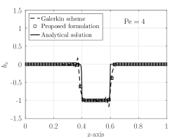
(a)

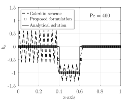
(b)

Figure 1: Comparison of simulation results for the 1D moving conductor problem (a) Pe = 4, (b) Pe = 400.

TABLE I: Measured values of error in $b_{x}=-dA_{y}/dz$ (first derivative) with the proposed formulation for 1D moving conductor problem with $\mu\sigma u_{z}=1000$

Number of	L2	Absolute	Expt. Order of
Elements	error	error	Convergence
50	2.49e-03	2.04e-02
100	1.76e-03	1.05e-02	0.96
200	1.21e-03	5.40e-03	0.95
400	7.84e-04	2.64e-03	1.03
800	4.50e-04	1.29e-03	1.04

In table I, the absolute and the root mean-squared (rms - L2) values of errors are displayed along with the experimental order of convergence. The errors are calculated for the reaction magnetic field $b_{x}=-dA_{y}/dz$, which is a quantity of interest in the moving conductor simulations. It can be seen that the weighted residual formulation provides stable as well as converging results for the 1D case.

The stability of the weighted residual formulation of (3), (II) are due to the non-oscillatory poles/roots present in the difference equation. This is in contrast to the stable formulations presented in [3, 24], where the stability of the formulation is achieved by canceling the oscillatory poles with the help of zeros of the input magnetic field. Therefore, the formulations of [3, 24] depends on the representation of the input magnetic field for the stability, while the formulation presented in (3), (II) are not dependent on the input magnetic field. Given this situation, it may be worthwhile to check the stability of the formulation for the transport equation. This is carried out in the next subsection.

II-C Simulation results from 1D transport equation

The transport equation describes the transport of a physical variable $\psi$ by means of advection and diffusion. The amount of diffusion is described by the diffusivity parameter $k$ and $u$ is the velocity of motion. The transport equation with the source term $S$ is given by,

$$-k\dfrac{d^{2}\psi}{dz^{2}}+u\dfrac{d\psi}{dz}=S$$ (10)

The weighted residual formulation can be written as,

$$\int_{\Omega}\dfrac{dN}{dz}\dfrac{d\psi}{dz}~{}d\Omega+\dfrac{u}{k}\int_{\Omega}NF_{z}~{}d\Omega=\dfrac{1}{k}\int_{\Omega}NS~{}d\Omega$$ (11)

$$-\int_{\Omega}\dfrac{dN}{dz}\dfrac{dF_{z}}{dz}~{}d\Omega+\dfrac{u}{k}\int_{\Omega}\dfrac{dN}{dz}\dfrac{d\psi}{dz}~{}d\Omega=\dfrac{1}{k}\int_{\Omega}\dfrac{dN}{dz}S~{}d\Omega$$ (12)

where, $N$ is the shape function and $F_{z}$ is the flux, defined as $F_{z}=d\psi/dz$. For the simulation, two standard test cases are considered. The first test problem (TP1) has source term $S=0$ and $\psi=0$ at $z=0$ and $\psi=1$ at $z=1$. The $u/k$ ratio is taken to be 400 for this test case. The second test problem (TP2) has source term $S=z^{2}$ and $\psi=0$ at $z=0$ and $z=1$. The $u/k$ ratio is taken to be 200 for this second test case.

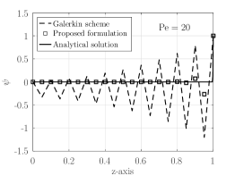
(a)

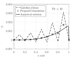
(b)

Figure 2: Comparison of simulation results for the 1D transport equation (a) TP1 (b) TP2

TABLE II: Error in $\psi$ with the proposed formulation for TP1 and TP2

	Number of	L2	Absolute	Expt. Order of
	Elements	error	error	Convergence
	20	4.15e-03	2.62e-02
	40	2.53e-03	1.16e-02	1.18
TP1	80	1.31e-03	4.24e-03	1.45
	160	5.08e-04	1.07e-03	1.99
	320	1.55e-04	2.44e-04	2.13
	10	1.40e-05	9.16e-05
	20	8.55e-06	4.04e-05	1.18
TP2	40	4.42e-06	1.47e-05	1.46
	80	1.72e-06	3.74e-06	1.98
	160	5.23e-07	8.59e-07	2.12

The simulation results are displayed in figure 2. The results show that the proposed formulation performs better than the Galerkin scheme. However, the absolute stability observed in the moving conductor problem (see figure 1) is not observed for the transport equation. This can be attributed to the hard boundary conditions set at either end of the simulation, which introduces a steep slope near the boundary.

The table II, displays the absolute and rms errors obtained from the weighted residual formulation for the first and second cases. The errors are calculated for the variable $\psi$, by comparing it with the respective analytical solution. The results show the expected experimental order of convergence for the weighted residual formulation.

Thus, even though the proposed formulation did not perform to 100%, the overall accuracy is achieved for the transport equation. It may be noted that for the 1D problems discussed so far, the upwinding formulations, such as the Streamline upwinding/Petrov-Galerkin (SU/PG) scheme would provide a highly accurate solution; close to the analytical solution. This is due to the fact that the upwinding stabilization parameter is derived by matching the numerical formulation with the analytical solution [5]. In the next section, analysis for the 2D moving conductor problems are described.

III Analysis with 2D moving conductor problems

The moving conductor problems, when described in two dimensions can exhibit two kinds of circulations; i) circulation of vector potential or current ii) circulation of magnetic field. This is due to the curl nature of the governing equation and it can be written as follows [3, 23]:

$$\sigma\nabla\phi~{}-~{}(\nabla\cdot\dfrac{1}{\mu}\nabla){\bf{A}}-\sigma~{}{\bf{u}}\times\nabla\times{\bf{A}}=\sigma~{}{\bf{u}}\times{\bf{B_{a}}}$$ (13)

$$\begin{split}\nabla\cdot(\sigma\nabla\phi)-\nabla\cdot(\sigma~{}{\bf{u}}\times\nabla\times{\bf{A}})=\nabla\cdot(\sigma~{}\bf{u}\times\bf{B_{a}})\end{split}$$ (14)

where, ${\bf u}$ is the velocity and $\phi$ is the electric scalar potential. In next subsection, the weighted residual formulation for a problem containing the circulation of vector potential or current is described.

III-A 2D problem with the circulation of A

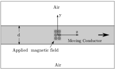
Figure 3: Schematic of the 2D moving conductor problem with the circulation of $\bf A$

The schematic of the 2D problem is shown in Fig. 3. The problem is defined along the $zy-$axis. The input magnetic field is directed perpendicular to the plane and it is directed along the x-axis ($B_{x}^{a}$). The conductor of width $d$ is moving along the $z$-axis with the velocity $u_{z}$. The simulation boundaries are chosen to be far from the input magnetic field.

In this problem, conductor motion creates a reaction magnetic field $b_{x}$, which tries to cancel the input magnetic field following the Lenz’s law. Therefore the current circulation and the circulation of the magnetic vector potential ${\bf A}$ are along the $zy-$plane and it has two components, $A_{y}$ and $A_{z}$. The governing equations of this problem can be written as [24],

$$\sigma\nabla^{2}\phi+\sigma u_{z}\dfrac{\partial^{2}A_{y}}{\partial y\partial z}-\sigma u_{z}\dfrac{\partial^{2}A_{z}}{\partial y^{2}}=\sigma u_{z}\dfrac{\partial B_{x}}{\partial y}$$ (15)

$$\sigma\dfrac{\partial\phi}{\partial y}-\dfrac{1}{\mu}\nabla^{2}A_{y}+\sigma u_{z}\dfrac{dA_{y}}{dz}-\sigma u_{z}\dfrac{dA_{z}}{dy}=\sigma u_{z}B_{x}$$ (16)

$$\sigma\dfrac{\partial\phi}{\partial z}-\dfrac{1}{\mu}\nabla^{2}A_{z}=0$$ (17)

Here, the first derivative term is arising from ${\bf u}\times\nabla\times{\bf A}$. This term can be rewritten as ${\bf u}\times{\bf b}$, following the 1D problem defined in equations (3), (II). In this problem, $\bf A$ has the circulation and only the x-component of the reaction magnetic field $b_{x}$ exists. In other words, the equations (16), (17) when written in terms of $b_{x}$, they become 2 equations and one unknown - $b_{x}$. Therefore, this is taken into account in the formulation of the weighted residual scheme.

The Galerkin finite element formulation of the equations (15), (16), (17) are written below with $N$ as weight (shape) function and the integration-by-parts is applied to second-derivative terms. Also, similar to the 1D case, the ${\bf u}\times\nabla\times{\bf A}$ is replaced with the ${\bf u}\times{\bf b}$ term.

$$\int_{\Omega}\sigma\nabla N\cdot\nabla\phi~{}d\Omega-\int_{\Omega}\sigma u_{z}\dfrac{\partial N}{\partial y}b_{x}~{}d\Omega=\int_{\Omega}\sigma u_{z}\dfrac{\partial N}{\partial y}B_{x}^{a}~{}d\Omega$$ (18)

$$\int_{\Omega}\sigma N\dfrac{\partial\phi}{\partial y}~{}d\Omega+\dfrac{1}{\mu}\int_{\Omega}\nabla N\cdot\nabla A_{y}~{}d\Omega~{}\dots$$

$$-\int_{\Omega}\sigma u_{z}Nb_{x}~{}d\Omega=\int_{\Omega}\sigma u_{z}NB_{x}^{a}~{}d\Omega$$ (19)

$$\int_{\Omega}\sigma N\dfrac{\partial\phi}{\partial z}~{}d\Omega+\dfrac{1}{\mu}\int_{\Omega}\nabla N\cdot\nabla A_{z}~{}d\Omega=0$$ (20)

Now, following the 1D formulation (II), one can write two more equations from (16), (17) with the weight functions $\partial N/\partial z$, $-\partial N/\partial y$ respectively. The weight functions are chosen such that the formulation has bilinear form in either $\bf A$ or $\bf b$ or both. The two equations are then summed and form a single equation for the one extra unknown - $b_{x}$; it is written as,

$$\int_{\Omega}\sigma\dfrac{\partial N}{\partial z}\dfrac{\partial\phi}{\partial y}~{}d\Omega-\int_{\Omega}\sigma\dfrac{\partial N}{\partial y}\dfrac{\partial\phi}{\partial z}~{}d\Omega~{}\dots$$

$$+\dfrac{1}{\mu}\int_{\Omega}\nabla N\cdot\nabla b_{x}~{}d\Omega-\int_{\Omega}\sigma u_{z}\dfrac{\partial N}{\partial z}\nabla\times{\bf A}\cdot\hat{x}~{}d\Omega~{}\dots$$

$$=\int_{\Omega}\sigma u_{z}\dfrac{\partial N}{\partial z}B_{x}^{a}~{}d\Omega$$ (21)

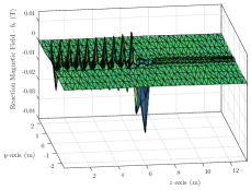
(a)

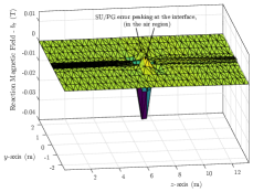
(b)

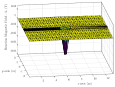
(c)

Figure 4: Reaction magentic field $b_{x}=dA_{z}/dy-dA_{y}/dz$ for the 2D moving conductor problem with the circulation of $\bf A$ (a) Galerkin scheme (b) SU/PG scheme [10, 22, 23] (c) Proposed formulation

TABLE III: Measured values of error in the reaction magnetic field $b_{x}=dA_{z}/dy-dA_{y}/dz$ with the proposed formulation for the 2D moving conductor problem with the circulation of $\bf A$

Number of	L2	Absolute	Expt. Order of
Elements	error	error	Convergence
10240	4.52e-06	4.44e-04
20480	2.85e-06	2.02e-04	1.14
40960	1.81e-06	9.83e-05	1.04
81920	1.01e-06	4.41e-05	1.16

The equations (18), (III-A), (20), (III-A) form the weighted residual formulation for this 2D case. Simulations are performed with bilinear quadrilateral elements, for different $Pe$ values and stable solutions are observed. A sample simulation plot is presented for $Pe=1500$ in Fig. 4, where Fig, 4a presents the solution from the Galerkin scheme and Fig. 4c presents the solution from the weighted residual formulation. In addition to this, an accuracy study is conducted and the results are presented in table III. In table III, the error in $\nabla\times{\bf A}$ is computed by comparing the solution with the solution obtained from a very fine discretisation. The error and the rate of convergence shows that the weighted residual formulation produces accurate and converging solutions for this 2D case. For quick comparison, Fig. 4b displays the result obtained from the SU/PG scheme. The magnetic field has the error peaking at the material interface and the peak occurs in the air-region adjacent to the moving conductor. This would lead to non-physical current circulation in the air-region [22, 23].

In the next subsection, the second case of the 2D moving conductor is described; where the circulation of the reaction magnetic field ${\bf b}$ is present, instead of the circulation of ${\bf A}$. For this, the ‘Testing Electromagnetic Analysis Methods’ (TEAM) problem No. 9a is chosen [25], and it is detailed in the next subsection.

III-B 2D problem with the circulation of b

A schematic representation of the TEAM-9a problem is provided in Fig. 7a. The TEAM-9a problem involves an infinite ferromagnetic material with the conductivity $\sigma=5\times 10^{6}~{}Sm^{-1}$ and the relative permeability of cases with $\mu_{r}=1,50$. The ferromagnetic material has a cylindrical bore of radius $r_{i}=14mm$. Inside the bore, a concentric current loop of diameter $r_{c}=12mm$ is carrying a current of $1A$ and it moves at an uniform velocity in the bore. This is an axisymmetric problem along the $z,~{}r$ axes, and it has no variation along the $\theta$-axis. For the analysis, the highest case with the velocity of $v=100ms^{-1}$ is considered. The finite element mesh is denser close to the current loop and becomes coarser as moving away from the current loop. The resulting $Pe$ varies from $5$ to $200$, due to the varying discretisation.

The coupled governing equation for this axisymmetric problem can be written in terms of the magnetic vector potential $A_{\theta}$ and the radial reaction magnetic field $b_{r}$ as,

$$-\dfrac{1}{\mu}\left(\dfrac{\partial^{2}A_{\theta}}{\partial r^{2}}+\dfrac{\partial^{2}A_{\theta}}{\partial z^{2}}+\dfrac{1}{r}\dfrac{\partial A_{\theta}}{\partial r}-\dfrac{A_{\theta}}{r^{2}}\right)-\sigma u_{z}b_{r}=\sigma u_{z}B_{r}^{a}$$ (22)

$$\dfrac{1}{\mu}\dfrac{\partial b_{r}}{\partial z}-\dfrac{\partial h_{z}}{\partial r}+\sigma u_{z}\dfrac{\partial A_{\theta}}{\partial z}=\sigma u_{z}B_{r}^{a}$$ (23)

where $z,~{}r$ are the axial and radial directions, $B_{r}^{a}$ is the radial component of the applied magnetic field due to the current carrying coil. In this problem, the reaction magnetic field has 2-components $b_{r}$, $b_{z}$. The moving conductor and the air medium has a jump in magnetic permeability. In this scenario, the component which is perpendicular to the moving conductor $\bf b_{\perp}$, is continuous across the conductor-air boundary. The parallel component is discontinuous across the boundary; however, the parallel component of magnetic field intensity ${\bf h_{\parallel}}$ is continuous across the conductor-air boundary. Thus the variables $b_{r}$ and $h_{z}$ are continuous in this problem. By following the 1D case in (3), (II) the weighted residual formulation for this 2D problem can be obtained. The (22) is weighted with the Galerkin weight function $N$ and the (23) is weighted with the weight function $\partial N/\partial z$. In addition to this, there is another variable $h_{z}$ present in in this formulation. For that,

$$\int_{\Omega}N\left(\dfrac{\partial A_{\theta}}{\partial r}+\dfrac{A_{\theta}}{r}\right)-\int_{\Omega}N\mu h_{z}=0$$ (24)

The third equation (24) is the Galerkin formulation for the parallel component $\bf h_{\parallel}$ and it is expressed as,

$$\nabla\times{\bf A}\cdot{\bf r_{\parallel}}-\mu{\bf h}\cdot{\bf r_{\parallel}}=0$$

where, $\bf r_{\parallel}$ is the tangent vector along the conductor-air boundary.

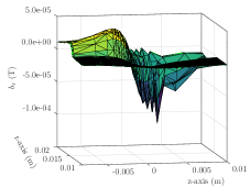
(a)

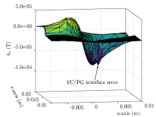
(b)

(c)

Figure 5: Simulation results from the 2D TEAM 9a problem for $u_{z}$ = 100 $ms^{-1}$ and $\mu_{r}$ = 50 case (a) Galerkin scheme - reaction magnetic field - $b_{r}$ (b) SU/PG scheme - reaction magnetic field - $b_{r}$ (c) Proposed formulation - reaction magnetic field - $b_{r}$

Simulations are carried out for the TEAM-9a problem, by using the 2280 bilinear quadrilateral elements. The results for the $u_{z}=100ms^{-1}$ and $\mu_{r}=50$ case is shown in Fig. 5. In this, the Fig. 5a shows the $b_{r}$ obtained from the Galerkin scheme and Fig. 5c shows the $b_{r}$ obtained from the weighted residual formulation. It can be seen that the solution from the proposed formulation is stable. For quick comparison, Fig. 5b displays the result obtained from the SU/PG scheme, showing the error peaking near the interface.

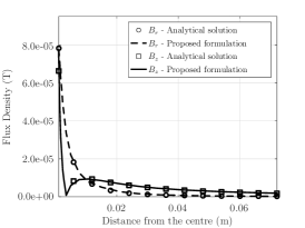
(a)

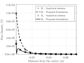
(b)

Figure 6: Comparison of the total magnetic flux densities from the analytical solution of the 2D TEAM 9a problem and the proposed formulation; for the cases of (a) $u_{z}=100ms^{-1}$, $\mu_{r}=1$ (b) $u_{z}=100ms^{-1}$, $\mu_{r}=50$

The accuracy of the formulation can be seen from Fig. 6, where the analytical solution of [25] is compared with the solution from the weighted residual formulation. In Fig. 6a, the comparison is made for the non-magnetic conductor and the velocity of $u_{z}=100ms^{-1}$; and in Fig. 6b, the comparison is made for the conductor with $\mu_{r}=50$ and the velocity of $u_{z}=100ms^{-1}$. In the next subsection, the weighted residual formulation for the 3D case is described.

IV 3D simulation of TEAM-9a problem

The coupled form of the governing equations for the 3D moving conductor problem can be written as [23, 24],

$$\nabla\cdot(\sigma\nabla\phi)-\nabla\cdot(\sigma~{}{\bf{u}}\times\nabla\times{\bf{A}})=\nabla\cdot(\sigma~{}\bf{u}\times\bf{B^{a}})$$ (25)

$$\sigma\nabla\phi~{}-~{}(\nabla\cdot\dfrac{1}{\mu}\nabla){\bf{A}}-\sigma~{}{\bf{u}}\times{\bf{b}}=\sigma~{}{\bf{u}}\times{\bf{B^{a}}}$$ (26)

$$\sigma\nabla\phi~{}+~{}\nabla\times\dfrac{\bf b}{\mu}-\sigma~{}{\bf{u}}\times\nabla\times{\bf{A}}=\sigma~{}{\bf{u}}\times{\bf{B^{a}}}$$ (27)

For the 3D case, the weighted residual formulation is similar to the 2D formulations presented above. In this, the (25), (26) have the Galerkin scheme with weight function $N$ and the (27) is weighted so as to have bilinear form in the formulation. Hence, the perpendicular components, ${\bf b}_{\perp}\rightarrow b_{x},b_{y}$ of (27) are weighted with the weight function $\partial N/\partial z$; and the parallel component, ${\bf h}_{\parallel}\rightarrow h_{z}$ is formulated as,

$$\int_{\Omega}N\left(\dfrac{\partial A_{y}}{\partial x}-\dfrac{\partial A_{x}}{\partial y}\right)-\int_{\Omega}N\mu h_{z}=0$$ (28)

which is similar to (24).

(a)

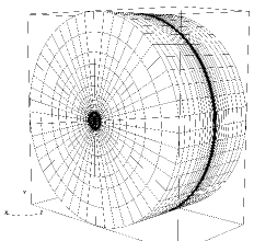
(b)

Figure 7: Description of the TEAM 9a problem (a) Schematic representation of the TEAM 9a moving conductor problem. (b) Finite element mesh employed

In order to test the formulation in 3D, the TEAM-9a problem in $x,y,z$-coordinate system is chosen. In the cartesian coordinates the TEAM-9a problem loses its symmetry and becomes a 3D test case with the materials having different permeability and conductivity. The results from the 2D simulation, can serve as a reference to test the correctness of the solution obtained from the 3D case. The schematic of the problem in 3D is shown in Fig. 7a. The simulation is carried out with 72000 trilinear hexahedron elements and its finite element mesh is shown in Fig. 7b.

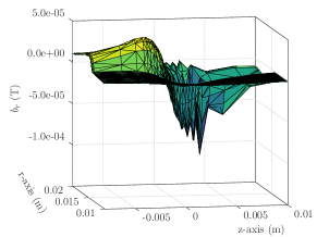
(a)

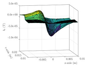
(b)

Figure 8: Simulation results ($b_{r}$) from the 3D TEAM 9a problem, at the cross-section along the $\theta\approx 0$ plane, for $u_{z}$ = 100 $ms^{-1}$ and $\mu_{r}$ = 50 case (a) Galerkin scheme (b) Proposed formulation

The reaction magnetic field along the radial direction is plotted in Fig. 8. The values are taken along the $\theta\approx 0^{o}$ plane. When comparing the Fig. 8 with the Fig. 5, it can be seen that the 3D results exactly resemble the results obtained from the 2D case. It may be noted that for the 3D problem, the axial $z$ and radial $r$ discretisations are kept nearly identical to the 2D case. Upon varying the angular discretisation, it is observed that the results from the 3D simulations are becoming more accurate with the increasing angular discretisation. Apart from accuracy, it can also be easily noted that the result from weighted residual formulation is stable (see Fig. 8b). Thus, the proposed formulation performs consistently in 3D as well.

V Discussion

The formulation presented here, holds few desired characteristics which are absent in the existing schemes.

i) The formulation is parameter-free. In upwinding schemes, the stability and the accuracy of the formulation relies on the correct value of stabilization parameter [5, 26]. For the 1D problems, an accurate expression for the stabilization-parameter is derived by matching the analytical solution. Hence, for the 1D cases, the SU/PG scheme would perform better than the proposed formulation. However, for the 2D and 3D cases, the SU/PG scheme is known to suffer from the error at the transverse boundary [19, 20, 21, 22, 23]. To resolve this, iterative techniques are suggested in the literature; which require a repeated calculation of the FEM solution to arrive at the correct solution [26, 20, 21]. These iterative techniques make the problem non-linear and increases the computation burden by several times. The typical number of iterations is found to be around in $\sim 100s$ or more; some cases also found to be non-converging [21]. The presented formulation does not require a stabilization parameter and hence, it is free from such a computational burden to arrive at a stable and accurate solution for the moving conductor problems.

ii) The formulation does not require any special representation of the input magnetic field $\bf B^{a}$, unlike [3, 24]. This is because, the numerical stability is not brought in by the $pole-zero$ cancellation of the input magnetic field. The formulation is inherently stable and the source term can be of any form.

iii) It may be noted that the reaction magnetic field, which is the practical output of the simulation, is measured from $\nabla\times{\bf A}$ at the interior point(s) inside the element; instead of obtaining ${\bf b}$ or ${\bf h}$ from the auxiliary equation. This provides one consistent and simple way to obtain the magnetic field for cases involving multiple magnetic materials. Also, the equations are observed to be numerically coupled, providing the order of convergence of 1 for both $\nabla\times{\bf A}$ and, ${\bf b}$ or ${\bf h}$.

VI Summary and Conclusion

The classical Galerkin finite element method, when applied to moving conductor problems, is known to lose numerical stability. This is due to the inability of the central weighted schemes to handle the dominant first derivative in the governing equation. The common strategy is to upwind the formulation, to have more weight along the flow direction. The correct amount of the upwind is decided by the stabilization parameter $\tau$. Upwind schemes are known to have other issues and various solutions are suggested in the finite element literature, which include the iterative solution strategies [18, 19, 26].

In this work, a different route is taken for the simulation of linear moving conductor problems. The central weighting is retained and the first derivative is excluded, by having auxiliary equation(s). In this way, the formulation is not upwinded and remains parameter-free. The stability of the formulation is shown in 1D with the help of $Z$-transform, as well as, with the numerical examples. In addition to this, the accuracy and the stability of the formulation is shown with the help of different 1D and 2D cases; including the cases with materials having different conductivity and magnetic permeability. Then the formulation is verified with a 3D moving conductor simulation; stable and consistent solutions are observed.

Sethupathy Subramanian received the masters and doctrate degrees in electrical engineering from IISc, Bangalore, India in 2011 and 2017 respectively. He is currently pursuing his graduate research at the Department of Physics and Astronomy, University of Notre Dame, USA. His research interests, pertinent to electrical engineering, include computational electromagnetics, numerical stability, finite element and edge element methods.

Sujata Bhowmick received the B.E. degree in electrical engineering from IIEST, Shibpur, India, in 2006, and the M.E. degree in electrical engineering from the IISc, Bengaluru, India, in 2011. She received the Ph.D. degree from the Department of Electronic Systems Engineering, IISc, Bengaluru, India, in 2019. Her research interests include power electronics for renewable resources, single-phase grid-connected power converters, computational electromagnetics, finite element and edge element methods.

References

- [1] E. Chan and S. Williamson, “Factors influencing the need for upwinding in two-dimensional field calculation,” Magnetics, IEEE Transactions on, vol. 28, no. 2, pp. 1611–1614, 1992.
- [2] T. Furukawa, K. Komiya, and I. Muta, “An upwind galerkin finite element analysis of linear induction motors,” Magnetics, IEEE Transactions on, vol. 26, no. 2, pp. 662–665, 1990.
- [3] S. Subramanian and U. Kumar, “Augmenting numerical stability of the galerkin finite element formulation for electromagnetic flowmeter analysis,” IET Science, Measurement & Technology, vol. 10, no. 4, pp. 288–295, 2016.
- [4] O. Zienkiewicz, R. Taylor, and P. Nithiarasu, The Finite Element Method for Fluid Dynamics. Elsevier Science, 2005.
- [5] T.-P. Fries and H. G. Matthies, “A review of petrov–galerkin stabilization approaches and an extension to meshfree methods,” Technische Universitat Braunschweig, Brunswick, 2004.
- [6] E. Oñate and M. Manzan, “Stabilization techniques for finite element analysis of convection-diffusion problems,” Developments in Heat Transfer, vol. 7, pp. 71–118, 2000.
- [7] D. Spalding, “A novel finite difference formulation for differential expressions involving both first and second derivatives,” International Journal for Numerical Methods in Engineering, vol. 4, no. 4, pp. 551–559, 1972.
- [8] A. Runchal, “Convergence and accuracy of three finite difference schemes for a two-dimensional conduction and convection problem,” International Journal for Numerical Methods in Engineering, vol. 4, no. 4, pp. 541–550, 1972.
- [9] I. Christie, D. F. Griffiths, A. R. Mitchell, and O. C. Zienkiewicz, “Finite element methods for second order differential equations with significant first derivatives,” International Journal for Numerical Methods in Engineering, vol. 10, no. 6, pp. 1389–1396, 1976.
- [10] A. N. Brooks and T. J. Hughes, “Streamline upwind/petrov-galerkin formulations for convection dominated flows with particular emphasis on the incompressible navier-stokes equations,” Computer methods in applied mechanics and engineering, vol. 32, no. 1, pp. 199–259, 1982.
- [11] M. Odamura, “Upwind finite element solution for saturated traveling magnetic field problems,” Electrical Engineering in Japan, vol. 105, no. 4, pp. 126–132, 1985.
- [12] D. Rodger, P. Leonard, and T. Karaguler, “An optimal formulation for 3d moving conductor eddy current problems with smooth rotors,” Magnetics, IEEE Transactions on, vol. 26, no. 5, pp. 2359–2363, 1990.
- [13] N. Allen, D. Rodger, P. Coles, S. Strret, and P. Leonard, “Towards increased speed computations in 3d moving eddy current finite element modelling,” Magnetics, IEEE Transactions on, vol. 31, no. 6, pp. 3524–3526, 1995.
- [14] D. Rodger, T. Karguler, and P. Leonard, “A formulation for 3d moving conductor eddy current problems,” Magnetics, IEEE Transactions on, vol. 25, no. 5, pp. 4147–4149, 1989.
- [15] L. Codecasa and P. Alotto, “2-d stabilized fit formulation for eddy-current problems in moving conductors,” Magnetics, IEEE Transactions on, vol. 51, no. 3, pp. 1–4, 2015.
- [16] Y. Liang, “Steady-state thermal analysis of power cable systems in ducts using streamline-upwind/petrov-galerkin finite element method,” Dielectrics and Electrical Insulation, IEEE Transactions on, vol. 19, no. 1, pp. 283–290, 2012.
- [17] S. Noguchi and S. Kim, “Magnetic field and fluid flow computation of plural kinds of magnetic particles for magnetic separation,” Magnetics, IEEE Transactions on, vol. 48, no. 2, pp. 523–526, 2012.
- [18] R. Codina, “A discontinuity-capturing crosswind-dissipation for the finite element solution of the convection-diffusion equation,” Computer Methods in Applied Mechanics and Engineering, vol. 110, no. 3, pp. 325–342, 1993.
- [19] T. J. Hughes, M. Mallet, and M. Akira, “A new finite element formulation for computational fluid dynamics: Ii. beyond supg,” Computer Methods in Applied Mechanics and Engineering, vol. 54, no. 3, pp. 341–355, 1986.
- [20] V. John and P. Knobloch, “On spurious oscillations at layers diminishing (sold) methods for convection–diffusion equations: Part i–a review,” Computer Methods in Applied Mechanics and Engineering, vol. 196, no. 17, pp. 2197–2215, 2007.
- [21] ——, “On spurious oscillations at layers diminishing (sold) methods for convection–diffusion equations: Part ii–analysis for p1 and q1 finite elements,” Computer Methods in Applied Mechanics and Engineering, vol. 197, no. 21, pp. 1997–2014, 2008.
- [22] S. Subramanian and U. Kumar, “Existence of boundary error transverse to the velocity in su/pg solution of moving conductor problem,” in Numerical Electromagnetic and Multiphysics Modeling and Optimization (NEMO), 2016 IEEE MTT-S International Conference on. IEEE, 2016, pp. 1–2.
- [23] S. Subramanian, U. Kumar, and S. Bhowmick, “On overcoming the transverse boundary error of the su/pg scheme for moving conductor problems,” IEEE Transactions on Magnetics, vol. 58, no. 1, pp. 1–8, 2021.
- [24] S. Subramanian and U. Kumar, “Stable galerkin finite-element scheme for the simulation of problems involving conductors moving rectilinearly in magnetic fields,” IET Science, Measurement & Technology, vol. 10, no. 8, pp. 952–962, 2016.
- [25] N. Ida, “Team problem 9 velocity effects and low level fields in axisymmetric geometries,” Proc. Vancouver TEAM Workshop, Jul. 1988.
- [26] E. Oñate, F. Zárate, and S. R. Idelsohn, “Finite element formulation for convective–diffusive problems with sharp gradients using finite calculus,” Computer methods in applied mechanics and engineering, vol. 195, no. 13, pp. 1793–1825, 2006.