New Photometric Calibration of the Wide Field Camera 3 Detectors

Abstract

We present a new photometric calibration of the WFC3-UVIS and WFC3-IR detectors based on observations collected from 2009 to 2020 for four white dwarfs, namely GRW+70 5824, GD 153, GD 71, G191B2B, and a G-type star, P330E. These calibrations include recent updates to the Hubble Space Telescope primary standard white dwarf models and a new reference flux for Vega. Time-dependent inverse sensitivities for the two WFC3-UVIS chips, UVIS1 and UVIS2, were calculated for all 42 full-frame filters, after accounting for temporal changes in the observed count rates with respect to a reference epoch in 2009. We also derived new encircled energy values for a few filters and improved sensitivity ratios for the two WFC3-UVIS chips by correcting for sensitivity changes with time. Updated inverse sensitivity values for the 20 WFC3-UVIS quad filters and for the 15 WF3-IR filters were derived by using the new models for the primary standards and the new Vega reference flux and, in the case of the IR detector, new flat fields. However, these values do not account for any sensitivity changes with time. The new calibration provides a photometric internal precision better than 0.5% for the wide-, medium-, and narrow-band WFC3-UVIS filters, 5% for the quad filters, and 1% for the WFC3-IR filters. As of October 15, 2020, an updated set of photometric keywords are populated in the WFC3 image headers.

1 Introduction

The Wide Field Camera 3 (WFC3) instrument was installed on the Hubble Space Telescope (HST) during the last servicing mission, Servicing Mission 4, on June 24, 2009.

WFC3 has greatly advanced the imaging capabilities of HST thanks to a combination of broad wavelength coverage, wide field of view, and high sensitivity. Composed of two optical/ultraviolet CCD detectors, or chips, UVIS1 and UVIS2, and a near-infrared (NIR) HgCdTe array, WFC3 can deliver high-resolution imaging over the wavelength range 2000 to 17000 Å  with a variety of wide-, intermediate-, and narrow-band filters. For more details on the detectors we refer the reader to the WFC3 Instrument Handbook.

The WFC3-UVIS detectors were built from two different CCD wafers and so have different quantum efficiencies, more significantly in the ultra-violet (UV) regime ($\lambda\lesssim$ 4,000 Å), where UVIS2 is more sensitive. In addition, the sensitivity of both detectors changes with time and the rate of change is different for each of them (Gosmeyer & Baggett 2016; Shanahan et al. 2017a; Khandrika et al. 2018, Calamida et al. 2021, hereinafter CA21). A change of sensitivity with time also seems to be present in the IR detector, the characterization of which is still ongoing (Bohlin et al. 2019; Kozhurina-Platais & Baggett 2020, Bajaj et al. 2020, hereinafter BA20).

In 2016, the WFC3 team implemented a chip-dependent photometric calibration and new values of the inverse sensitivities for UVIS1 and UVIS2 were provided (Deustua et al., 2016, hereinafter DE16), and later improved by using updated CALSPEC models for the HST primary spectrophotometric standard white dwarfs (WDs, Deustua et al. 2017b, hereinafter DE17). However, these values did not take into account the sensitivity change of the WFC3-UVIS detectors. As documented in Khandrika et al. (2018) and CA21, sensitivity changes are up to 0.2% per year, according to the filter and the chip, resulting in differences of more than 2% in flux between 2009, when WFC3 was installed, and the current epoch. Due to the sensitivity changes being different for UVIS1 and UVIS2, as well as small errors in the flat field between the four readout amplifiers, the 2017 ratios of the observed count rates across the UVIS1 and UVIS2 detectors were off by up to 2% for some filters (Calamida et al., 2018, hereafter CA18).

The CALSPEC models for the HST primary spectrophotometric standard WDs, GD153, GD71 and G191B2B, were updated in March 2020 (Bohlin et al., 2020, hereinafter BO20), and the Vega reference grey flux increased by $\approx$ 0.9%. Overall, the standard WD fluxes increased by $\approx$ 2% for wavelengths in the range 0.15 - 0.4 $\mu$m, and $\approx$ 1.5% in the range 0.4 - 1 $\mu$m. Therefore, WFC3-UVIS inverse sensitivities were updated in October 2020 to take into account these new CALSPEC reference fluxes and the different time sensitivity changes of the detectors. The 20 quad filter inverse sensitivities were also updated to incorporate the new models, but did not include any time-dependent correction since no observations in these filters are available beyond 2010.

The WFC3-IR inverse sensitivities were last presented in Kalirai et al. (2011), and were only based on the first 1.5 years of photometric measurements of the three HST primary standard WDs and the G-type standard P330E. In October 2020, the IR inverse sensitivities were updated by using all the observations collected through August 2020, the new CALSPEC models for the HST primary WDs, and the new Vega reference flux; however, no time-dependent correction was applied (BA20).

The new WFC3-UVIS and WFC3-IR photometric calibrations also include observations of the standard WD GRW70+70 5824 (hereinafter GRW70). An improved spectral energy distributions (SED) of GRW70, based on new STIS observations with the $G430L$ grating, was added to the CALSPEC database. The observed SED of GRW70 was upgraded to one of the best secondary HST standards: routine monitoring of this star with STIS, ACS and WFC3 showed similar time-dependent changes as seen for the three HST primary WDs (GD153, GD71, G191B2B), with no suggestion of systematic variability of GRW70 to within a limit of $\approx$1% (BO20, Bohlin 2022, private communication).

In this manuscript, we describe how the new inverse sensitivities for the 42 full-frame and the 20 quad WFC3-UVIS filters, and the 15 WFC3-IR filters were derived. In both cases, approximately 10 years of photometry collected for three primary and one secondary HST standard WDs, and the standard G-type star P330E were used. Their updated SEDs based on the new CALSPEC models were also used. More accurate encircled energy (EE) corrections were derived for a few WFC3-UVIS filters by normalizing the images using the newly derived time-dependent corrections and ratios. In this article, we also test the improved WFC3-UVIS photometric calibration by comparing multi-band and multi-epoch photometry for the Large Magellanic Cloud (LMC) open cluster NGC 1978 to a set of theoretical models.

The structure of the manuscript is as follows. In §2 we illustrate the observations used in this work and the data reduction process, in §3 we describe the data analysis process. §4 presents the new EE corrections for WFC3-UVIS while §5 describes the process to derive new in-flight corrections for UVIS1 and UVIS2, and §6 the process to derive the new inverse sensitivities for the WFC3-UVIS and IR detectors. §7 compares the new to the old inverse sensitivities and in §8 we validate the new WFC3-UVIS time-dependent photometric calibration. The next section provides an example on how to perform WFC3-UVIS flux calibration, and we summarize the results in §10.

2 Observations and data reduction

2.1 WFC3-UVIS

Observations for four CALSPEC standard WDs, GRW70, GD153, GD71, G191B2B, and the G-type standard star, P330E, were collected with WFC3-UVIS between June 2009 and November 2019 during calibration and a few General Observer (GO) programs.

The WFC3-UVIS detectors, UVIS1 and UVIS2, are $4k\times 2k$ CCDs with a pixel scale of 0.04″/pixels, for a total combined field of view of 162″$\times$ 162″. Each detector is divided in two amplifiers, A and B on UVIS1, and C and D on UVIS2. A scheme of the WFC3-UVIS detector and its amplifiers can be found in Fig. 1.2 of Section 1.2 of the Data Handbook.

Using a range of available sub-arrays, targets may be positioned on specific regions of the detector, and the total observing overhead is reduced by reading out only a fraction of the array. In order to mitigate the effects of charge transfer inefficiency, sub-arrays are defined at each of the UVIS detector corners closest to the readout amplifiers (see Section 6.4 of the Instrument handbook for details). For the WFC3 flux calibration, the five CALSPEC standards are typically observed in the smallest 512$\times$512 pixel corner sub-arrays, namely UVIS1-C512A-SUB (on amplifier A), UVIS1-C512B-SUB (B), UVIS2-C512C-SUB (C), and UVIS2-C512D-SUB (D). Two sub-array positions are observed for each detector in order to check the accuracy of the flat field calibration.

Exposure times for each filter were optimized to obtain a minimum Signal-to-Noise ratio ($S/N$) of $\approx$ 100, and on average $S/N\approx$ 500 per exposure. Table LABEL:table:1 lists the proposal program numbers, the standard star names and filters for the observations included in this work.

Images were processed through the WFC3 pipeline, calwf3, version 3.5.0, which used the image photometry table (IMPHTTAB) available in November 2019, 1681905hi_imp.fits, which corresponds to the latest WFC3-UVIS photometric calibration of DE17. calwf3 processes the images through the bias correction, dark subtraction, flat-fielding, gain conversion and charge transfer efficiency (CTE) correction. calwf3 version 3.5.0 used the original version of the CTE correction (Anderson & Baggett, 2014) and the PCTETAB zcv2057mi_cte.fits; a new CTE correction was implemented in April 2021 by the WFC3 team and is currently available with calwf3 version 3.6.0 and later (Anderson et al., 2021), and uses the PCTETAB 54l1347ei_cte.fits.

Standard stars were observed in the four UVIS 512$\times$512 corner sub-arrays, positioned close to the readout amplifiers, where the charge transfer inefficiency effects are smaller. Also, all the observed standards are bright ($V\lesssim$ 13.5 mag), and so less affected by the charge transfer inefficiency. However, we decided to test the effect of the new CTE correction on the standard star observations. We processed several images of GRW70 in a few filters with both the old and the new CTE correction. Aperture photometry was performed by using the same parameters and results were compared: count rates for GRW70 differed by no more than $\approx$ 0.01% in all the filters examined.

The _flc images processed through calwf3 were also multiplied by the pixel area map (PAM, Kalirai et al. 2010), to correct for differences in the area of each pixel on the sky due to the geometric distortion of the UVIS1 and UVIS2 detectors.

Table 1: Program number of the regular calibration or GO proposal, standard star name and filters for the WFC3-UVIS observations included in this analysis. These data can be found on the MAST archive by using the following DOI: 10.17909/gvre-t314.

Program	Star	Filters
11426	GRW70	F218W	F225W	F275W	F280N	F300X	F336W	F343N	F373N	F390M	F390W	F395N	F410M
										F438W	F467M	F606W	F814W
11450		F218W	F225W	F275W	F280N	F300X	F336W	F343N	F350LP	F373N	F390M	F390W	F395N
	GD153	F410M	F438W	F467M	F469N	F475W	F475X	F487N	F502N	F547M	F555W	F600LP	F606W
		F621M	F625W	F656N	F658N	F665N	F673N	F689M	F763M	F775W	F814W	F845M	F953N
11557	GRW70												F475W
		F200LP	F218W	F225W	F275W	F280N	F300X	F336W	F343N	F350LP	F373N	F390M	F390W
		F395N	F410M	F438W	F467M	F469N	F475W	F475X	F487N	F502N	F547M	F555W	F600LP
	G191B2B	F606W	F621M	F625W	F631N	F645N	F656N	F657N	F658N	F665N	F673N	F680N	F689M
								F763M	F775W	F814W	F845M	F850LP	F953N
11903	GD153	F225W	F275W	F336W	F350LP	F390W	F438W	F467M	F469N	F475W	F502N	F547M	F555W
										F606W	F775W	F814W	F850LP
	GD71	F350LP	F390W	F438W	F467M	F469N	F475W	F502N	F547M	F555W	F606W	F775W	F814W
													F850LP
	P330E	F200LP	F218W	F225W	F275W	F300X	F336W	F350LP	F390W	F410M	F438W	F467M	F475W
			F475X	F547M	F555W	F600LP	F606W	F621M	F625W	F689M	F775W	F814W	F850LP
11907	GRW70		F218W	F225W	F275W	F336W	F390M	F390W	F438W	F475W	F547M	F606W	F814W
12333	GRW70	F218W	F225W	F275W	F300X	F336W	F390M	F390W	F438W	F467M	F469N	F475W	F502N
									F547M	F555W	F606W	F814W	F850LP
12698	GRW70	F218W	F225W	F275W	F300X	F336W	F390M	F390W	F438W	F467M	F475W	F502N	F547M
										F555W	F606W	F814W	F850LP
13088	GRW70						F218W	F225W	F275W	F336W	F438W	F606W	F814W
		F200LP	F218W	F225W	F275W	F280N	F300X	F336W	F343N	F350LP	F373N	F390M	F390W
	GD153	F395N	F410M	F438W	F467M	F469N	F475W	F475X	F487N	F502N	F547M	F555W	F600LP
		F606W	F621M	F625W	F631N	F645N	F656N	F657N	F658N	F665N	F673N	F680N	F689M
13089								F763M	F775W	F814W	F845M	F850LP	F953N
		F200LP	F218W	F225W	F275W	F280N	F300X	F336W	F343N	F350LP	F373N	F390M	F390W
	P330E	F395N	F410M	F438W	F467M	F469N	F475W	F475X	F487N	F502N	F547M	F555W	F600LP
		F606W	F621M	F625W	F631N	F645N	F656N	F657N	F658N	F665N	F673N	F680N	F689M
								F763M	F775W	F814W	F845M	F850LP	F953N
13574	GRW70						F218W	F225W	F275W	F336W	F438W	F606W	F814W
		F200LP	F218W	F225W	F275W	F280N	F300X	F336W	F343N	F350LP	F373N	F390M	F390W
	GD153	F395N	F410M	F438W	F467M	F469N	F475W	F475X	F487N	F502N	F547M	F555W	F600LP
		F606W	F621M	F625W	F631N	F645N	F656N	F657N	F658N	F665N	F673N	F680N	F689M
13575								F763M	F775W	F814W	F845M	F850LP	F953N
		F200LP	F218W	F225W	F275W	F280N	F300X	F336W	F343N	F350LP	F373N	F390M	F390W
	P330E	F395N	F410M	F438W	F467M	F469N	F475W	F475X	F487N	F502N	F547M	F555W	F600LP
		F606W	F621M	F625W	F631N	F645N	F656N	F657N	F658N	F665N	F673N	F680N	F689M
								F763M	F775W	F814W	F845M	F850LP	F953N
13711	G191B2B								F275W	F336W	F475W	F625W	F775W
	GD153								F275W	F336W	F475W	F625W	F775W
	GD71								F275W	F336W	F475W	F625W	F775W
		F200LP	F218W	F225W	F275W	F300X	F336W	F350LP	F390M	F390W	F410M	F438W	F467M
	G191B2B	F475W	F475X	F547M	F555W	F600LP	F606W	F621M	F625W	F689M	F763M	F775W	F814W
14018												F845M	F850LP
	GRW70	F218W	F225W	F275W	F300X	F336W	F390M	F390W	F410M	F438W	F467M	F475W	F547M
										F555W	F606W	F814W	F850LP
14021	GD153	F218W	F225W	F275W	F336W	F350LP	F438W	F475W	F547M	F555W	F600LP	F606W	F621M
										F625W	F775W	F814W	F845M
	P330E	F275W	F336W	F350LP	F438W	F475W	F547M	F555W	F600LP	F606W	F621M	F625W	F775W
											F814W	F845M	F850LP
	G191B2B	F218W	F225W	F275W	F336W	F438W	F475W	F547M	F555W	F600LP	F606W	F621M	F625W
											F775W	F814W	F845M
	GD153	F218W	F225W	F275W	F336W	F350LP	F438W	F475W	F547M	F555W	F600LP	F606W	F621M
14384										F625W	F775W	F814W	F845M
	GD71	F218W	F225W	F275W	F336W	F350LP	F438W	F475W	F547M	F555W	F600LP	F606W	F621M
										F625W	F775W	F814W	F845M
	P330E	F275W	F336W	F350LP	F438W	F475W	F547M	F555W	F600LP	F606W	F621M	F625W	F775W
											F814W	F845M	F850LP
14815	GD153						F218W	F225W	F275W	F336W	F438W	F606W	F814W
	GRW70						F218W	F225W	F275W	F336W	F438W	F606W	F814W
	G191B2B	F218W	F225W	F275W	F336W	F438W	F475W	F547M	F555W	F600LP	F606W	F621M	F625W
											F775W	F814W	F845M
	GD153	F218W	F225W	F275W	F336W	F350LP	F438W	F475W	F547M	F555W	F600LP	F606W	F621M
14883										F625W	F775W	F814W	F845M
	GD71	F218W	F225W	F275W	F336W	F350LP	F438W	F475W	F547M	F555W	F600LP	F606W	F621M
										F625W	F775W	F814W	F845M
	P330E	F275W	F336W	F350LP	F438W	F475W	F547M	F555W	F600LP	F606W	F621M	F625W	F775W
											F814W	F845M	F850LP
	G191B2B	F218W	F225W	F275W	F336W	F438W	F475W	F547M	F555W	F606W	F621M	F625W	F657N
											F775W	F814W	F953N
	GD153	F218W	F225W	F275W	F336W	F350LP	F438W	F475W	F547M	F555W	F600LP	F606W	F621M
14992									F625W	F657N	F775W	F814W	F845M
	GD71	F218W	F225W	F275W	F336W	F438W	F475W	F547M	F555W	F606W	F621M	F625W	F657N
											F775W	F814W	F953N
	P330E	F275W	F336W	F350LP	F438W	F475W	F547M	F555W	F600LP	F606W	F621M	F625W	F775W
											F814W	F845M	F850LP
	G191B2B								F275W	F336W	F475W	F625W	F775W
15113	GD153								F275W	F336W	F475W	F625W	F775W
	GD71								F275W	F336W	F475W	F625W	F775W
15398	GD153						F218W	F225W	F275W	F336W	F438W	F606W	F814W
	GRW70						F218W	F225W	F275W	F336W	F438W	F606W	F814W
15399	GD153							F218W	F225W	F275W	F336W	F606W	F814W
	P330E							F218W	F225W	F275W	F336W	F606W	F814W
	GD153	F218W	F225W	F275W	F336W	F438W	F475W	F547M	F555W	F606W	F621M	F625W	F657N
											F775W	F814W	F845M
	GD71	F218W	F225W	F275W	F336W	F438W	F475W	F547M	F555W	F606W	F621M	F625W	F657N
15582											F775W	F814W	F953N
	P330E	F275W	F336W	F350LP	F438W	F475W	F547M	F555W	F600LP	F606W	F621M	F625W	F775W
											F814W	F845M	F850LP
	GRW70	F218W	F225W	F275W	F336W	F438W	F475W	F547M	F555W	F606W	F621M	F625W	F657N
											F775W	F814W	F953N
15583	GD153						F218W	F225W	F275W	F336W	F438W	F606W	F814W
	GRW70						F218W	F225W	F275W	F336W	F438W	F606W	F814W

A Python pipeline based on Photutils and WFC3_tools was developed to perform photometry on the thousands of images available. Below we provide a description of the pipeline steps that produce photometric catalogs for each standard star and filter.

1) The PAM-corrected _flc images were divided by the exposure time to convert total counts (e^-) to count rates (e^-/s);

2) Standard stars in calibration programs are usually observed close to the center of the 512$\times$512 sub-array; therefore, a first attempt to detect the star near the center of the sub-array wass done by using a segmentation map. Images were smoothed with a 3$\times$3 pixel kernel with a Full Width Half Maximum (FWHM) of 1.8 pixels. A detection threshold of 30 and 100 connected pixels was found to work for all images to find most stars on the first try. If no sources were found, the detection parameters were adjusted, i.e. the threshold was set to 15 and the connection pixels to 75, and the segmentation map was created again. If the second try failed, the image was discarded; however, this happened in a very small fraction of data, $\leq$ 2%. In the case where two or more sources were found, a method was devised to determine which of those was the standard star. The image header keywords RA_TARG and DEC_TARG were compared to the coordinates of the detected standard, RA and DEC. Since the proper motion information was not included in the calibration proposals for pre-2015 data, astroquery was used to query SIMBAD for the proper motion of the standard star and these were applied to RA_TARG and DEC_TARG. The detected source with coordinates closest to the corrected target location was selected as the standard star;

3) The sky background and sky root mean square (RMS) were calculated as the sigma-clipped mean of the pixels in a circular annulus of 9 pixels in width, with an inner radius of 156 pixels centered on the detected standard star. The sky background was then subtracted from the source count rates;

4) Aperture photometry was measured at different aperture radii, from 1 to 50 pixels, centered on the standard star;

5) Photometric errors were computed by following the prescription of Stetson (1987), i.e. including Poisson, sky background and readout noises;

6) Outlier measurements were defined as those more than 5% away from the median count rate value of the standard star on all the _flc exposures for each filter and amplifier; these were clipped before the catalogs were finalized. This cleaning enabled the removal of images impacted by cosmic ray (CR) hits on the source Point-Spread Function (PSF) or of poor measurements.

2.1.1 Scanned photometry

WFC3-UVIS spatial scan observations for two of the four WDs, namely GRW70 and GD153, were also included in the analysis to measure the sensitivity change of the UVIS1 and UVIS2 detectors with time. Spatial scans of bright sources, when compared to staring mode observations, are expected to yield higher precision photometry. Scans allow the collection of millions of source photons without causing saturation by spreading them across many pixels on the detector, and, thereby, reducing the Poisson noise. Averaging over a large number of pixels also helps to reduce noise originating from spatial effects such as bad pixels and flat-field errors. Indeed, it has been determined that sub-0.1% photometric repeatability is possible with spatial scans (Shanahan et al., 2017b).

Table 2: Program number of the regular calibration proposals, standard star name and filters for the WFC3-UVIS spatial scan observations included in this analysis. These data can be found on the MAST archive by using the following DOI: 10.17909/q0m5-n042.

Program	Star	Filters
14878	GRW70	F218W	F225W	F275W	F336W	F438W	F606W	F814W
	GD153	F218W	F225W	F275W	F336W	F438W	F606W	F814W
15398	GRW70	F218W	F225W	F275W	F336W	F438W	F606W	F814W
	GD153	F218W	F225W	F275W	F336W	F438W	F606W	F814W
15583	GRW70	F218W	F225W	F275W	F336W	F438W	F606W	F814W
	GD153	F218W	F225W	F275W	F336W	F438W	F606W	F814W

Spatial scan data were collected during four calibration proposals between 2017 and 2020; Table 2 lists the program numbers, the standard star names and the filters of the scan observations used in this analysis. Program 14878 was exploratory and examined the viability of using spatial scans as a high-precision technique for studying temporal photometric stability. An optimal observing strategy, based on the results from this program, was established by Shanahan et al. (2017b), and all the observations included in this work were obtained following their prescriptions. Data were acquired using either the UVIS1-C512A-SUB or the UVIS2-C512C-SUB sub-array.

As in the staring mode reduction process described above, raw scan images were processed through the calwf3 pipeline version 3.5.0, by using the IMPHTTAB 1681905hi_imp.fits, so that bias correction, dark subtraction, flat-fielding and gain conversion were performed. However, unlike the staring mode data, scan images were not corrected for the charge transfer inefficiency effects since these are minimal in the bright spatial scan trails centered within sub-arrays close to the readout amplifiers. To further mitigate these effects, scans were executed in the vertical direction along the detector columns. In addition, scans were inclined by a 1^∘ angle to uniformly sample the pixel phase for each CCD.

The _flt image products were then processed by a multi-step reduction pipeline introduced and described fully in Shanahan et al. (2017b). In summary, this Python based pipeline utilizes various tools from scientific data analysis packages such as astropy and Photutils, and performed the following steps:

1) CR detection and repair - Longer exposure times and the spreading of source flux over a large area on the detector make the spatial scans more susceptible to CR hits compared to the staring mode observations. Building on a routine originally developed for CR identification in Space Telescope Imaging spectrograph (STIS) CCD images, this step identified CR events in the data. The affected pixels were then repaired by interpolating from unaffected neighboring pixels;

2) Determining the scan location - Each image was designed to have the single-lined, vertical scan positioned at the center of the 512$\times$512 sub-array. However, to account for small shifts, an automated determination of the scan centroid location was performed for each image. A simultaneous determination of the scan direction was also performed. However, as mentioned before, the entire dataset considered in this work comprises vertical scans only;

3) Sky background subtraction - The sky region corresponding to each vertical scan was defined as all pixels excluding a 10-pixel wide strip bordering the sub-array and a 350$\times$75 pixel rectangular region centered on the scan. The sky background level and the sky RMS were calculated as the sigma-clipped mean and RMS of all the sky pixels. This background was then subtracted from the data and the errors were propagated accordingly;

4) Scaling with pixel area maps - The sky subtracted image was scaled by applying the appropriate PAM to account for geometric distortions of the detector;

5) Aperture photometry - The last step in this process is to perform aperture photometry on the sky-subtracted, PAM corrected image to determine the sum of pixels in the scan. This was done using a 240$\times$36 pixel rectangular aperture placed at the scan centroid determined in step 2). The dimensions of the aperture were chosen such that it was large enough to contain the scan in its entirety, yet it was not too large to be affected by noise from the sky subtraction. In this regime of very high total source counts, the Poisson noise term should dominate and is therefore approximated as the measurement error. Finally, the photometric measurement was converted into source count rates (e^-/s) by dividing the sum of pixels by the image exposure time.

Table 3: Star name and program numbers for the WFC3-IR observations used in this analysis. These data can be found on the MAST archive by using the following DOI: 10.17909/04tn-rj35.

Stars	Program
GD153	11451	11552	11926	12334	12699	12702	13089	13092	13575	13579	13711
		14021	14384	14386	14544	14883	14992	14994	15113	15582	16030
GD71	11926	11936	12333	12334	12357	12699	12702	13711	14024	14384	14883
								14992	15113	15582	16030
GRW70					11557	12333	12698	13088	13575	15582	16030
P330E	11451	11926	12334	12699	13089	13573	13575	14021	14328	14384	14883
										14992	16030
G191B2B						11926	12334	13094	13576	13711	15113

2.2 WFC3-IR

Observations for four CALSPEC standard WDs and for the G-type standard star P330E were collected with WFC3-IR between June 2009 and August 2020 during regular calibration and a few GO programs in all the 15 filters.

WFC3-IR is a 1014$\times$1014 detector, with a pixel scale of 0.13″and a total field of view of 136″$\times$ 123″. Sub-arrays of different sizes are available for the observations at the center of the detector. Standard star images were collected by using these sub-arrays, with the size determined from the exposure time used;this ranged between 64 $\times$ 64 and 512 $\times$ 512 pixels (see Section 7.4 of the Instrument Handbook for more details on the different WFC3-IR sub-arrays).

As some of the programs were not designed for photometric calibration purposes, the number of observations for each target and filter varies. The list of programs in which data were taken for each star is presented in Table 3.

The majority of the datasets used in this analysis were observed as part of photometric calibration programs, and typically feature long enough exposure times to exceed a $S/N\gtrsim$ 100. Starting from 2017, the observations were designed to mitigate the effects of persistence, which is critical to achieve high-precision photometry. In particular, frequent dithering of at least 10 pixels was used to place the star on a recently unused portion of the detector (Bajaj, 2019).

Images were processed with calwf3 version 3.5.0 and the IMPHTAB wbj1825ri_imp.fits was used. New flat fields were delivered at the end of 2020 and were used in the image processing; these have errors $\lesssim$ 0.5% (Mack et al., 2021).

Images were grouped by target and filter, and those collected in the same visit were drizzled together, as images taken in the same visit typically have very precise relative astrometry. Drizzling reduced the number of discrepant artifacts in the images, such as CRs, hot and bad pixels.

Source finding was performed on the drizzled images by using the DAOFIND algorithm (Stetson, 1987) as implemented in the Python package Photutils. The FWHM was set to the width of the WFC3-IR PSF, i.e. $\approx$ 1.2 pixels. Though the FWHM varies slightly for different filters, a parametrization with respect to wavelength was unnecessary to achieve satisfactory results. Due to the highly undersampled nature of the WFC3-IR PSF, many spurious objects would often be detected on the drizzled image. In some cases, due to a larger sub-array and longer exposure times, other sources also appeared in the images, leading to extra detections. To dispense of the superfluous detections, an initial pass of aperture photometry was performed on the drizzled images. The measured count rates of all sources were then compared to synthetic count rates of the standard stars computed with Pysynphot by using the latest SEDs and the total system throughput curves. The object that reported the closest count rates to the synthetic ones was used to record an approximate position of the standard star in each drizzled image. This position was transformed from the drizzled to the _flt image coordinate system via the all_pix2world() and all_world2pix() methods of the WCS package within astropy (The Astropy Collaboration et al. (2018)). The position was then re-centered in each _flt image using a 2D gaussian fitting to the central-most pixels of the PSF, ensuring that the small aperture used in the photometry is placed correctly.

Aperture photometry was then performed on the PAM-corrected _flt images with an aperture radius of 3 pixels ($\approx$ 0.4″), a background annulus ranging from 15 to 30 pixels centered on the standard star, and using a $\sigma$-clipped median to calculate the sky background. Unlike the analysis in Kalirai et al. (2011), the PAM multiplication was necessary, as the placement of the stars on the images spanned much of the total detector area. Aperture photometry was perforemed by using Photutils and the wfc3_photometry package (Bradley et al., 2017). Since the _flt images for the IR channel are already in units of $e^{-}/s$, the exposure time corrections was not required. In Kalirai et al. (2011), the aperture radius of 3 pixels was used, but was described as not optimal for minimizing the dispersion of the measurements. However, in repeating this analysis with more data, we found that the 3-pixel aperture minimizes the standard deviation for GD153 (the most observed star of the set) flux measurements in both the $F110W$ and $F160W$ filters.

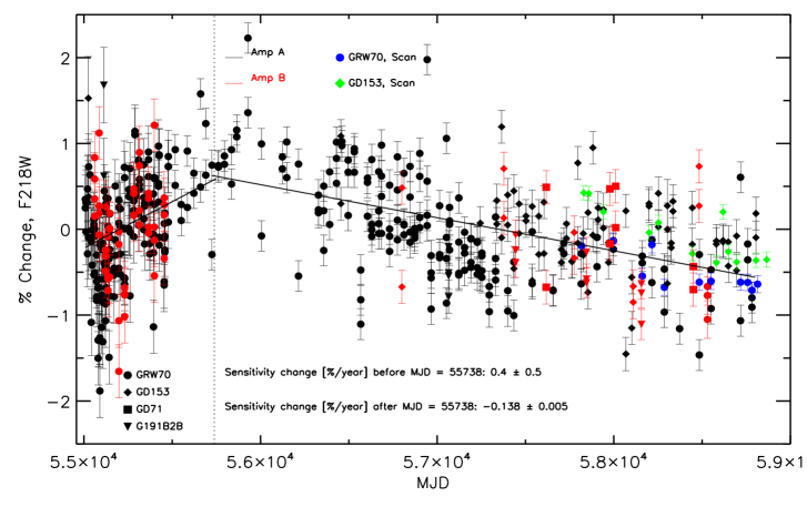
Figure 1: Aperture photometry performed with a 10-pixel radius on _flc images collected with the F218W filter and the UVIS1-C512A-SUB (Amp A, black) and UVIS1-C512B-SUB (Amp B, red) sub-arrays for four CALSPEC white dwarfs, namely GRW70 (filled circle), GD153 (diamond), GD71 (square), and G191B2B (triangle), is plotted as a percent change values versus the $MJD$ of the observations. Photometry performed on scan images in the same filter and for GRW70 (blue) and GD153 (green) is also shown. The solid lines show the fit to the photometry of all the stars before and after $MJD=$ 55738, indicated by a vertical dotted line. The sensitivity change rates in %/yr derived from fitting the data are labeled in the figure.

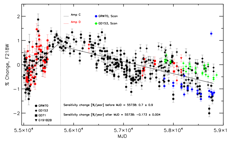
Figure 2: Same as Fig. 1 but for data collected with the UVIS2-C512C-SUB (Amp C, black) and the UVIS2-C512D-SUB (Amp D, red) sub-arrays.

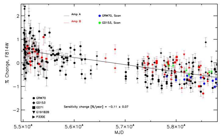
Figure 3: Same as Fig. 1 but for the $F814W$ filter. In this case, photometry for the CALSPEC G-type standard P330E (horizontal triangle) is also included.

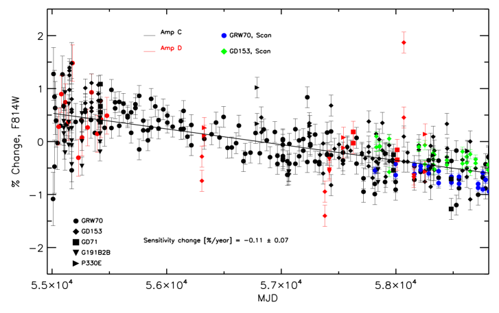
Figure 4: Same as Fig. 3 but for data collected with the UVIS2-C512C-SUB (Amp C, black) and the UVIS2-C512D-SUB (Amp D, red) sub-arrays.

3 Data Analysis

3.1 WFC3-UVIS

Aperture photometry with a 10-pixel radius for each standard star and filter was normalized to the mean value over the full time interval and the percent change of the count rates was plotted as a function of the Modified Julian Day ($MJD$) of the observation. The spatial scan photometry for GRW70 and GD153, when available, was normalized to the staring mode photometry at 10 pixel for the same stars in the same time interval, $\sim$ 55700 – 58800, i.e. $\sim$ 2016.8– 2019.8, and the percent change values were overplotted. This normalization was done by manually shifting the scan count rates to match the mean count rate of the staring mode of each observed standard star over the same time interval. The WFC3 team is currently testing new ’enrectangled’ energy corrections to be applied to synthetic count rates in order to compare them to the standard star observed count rates. This process is described in Section 2.1.1 and more details can be found in Marinelli et al. (2022, in prep.).

As shown in Figs. 1, 2, 3, and 4, small offsets between the photometry of different standard stars is present and is currently under investigation by the WFC3 team. We used these data to determine the best sensitivity change slopes for each filter and chip and then corrected the count rates of each standard star over time. The corrected count rates were then used to determine the final normalized photometry in all filters. Since most measurements were collected on Amps A and C, mean count rates on Amps B and D were normalized to the mean count rates on Amp A and C, respectively, in order to correct for small ($\lesssim$ 2%) errors in the flat-field across each chip (Mack et al., 2015).

Table 4: Slopes and their 1-$\sigma$ dispersion of the sensitivity changes for UVIS1 (Amp A) and UVIS2 (Amp C) 42 full-frame filters. The UV filters have two slopes, one for $MJD\leq$55738 and one for later times, while the redder filters have only one slope (see text for more details).

Filter	Pivot	Slope1/$\sigma$ ($MJD\leq$ 55738)	Slope2/$\sigma$ ($MJD>$ 55738)	Pivot	Slope1/$\sigma$ ($MJD\leq$ 55738)	Slope2/$\sigma$ ($MJD>$ 55738)
	(Å)	(%/yr)	(%/yr)		(%/yr)	(%/yr)
UVIS1 (Amp A)				UVIS2 (Amp C)
F200LP	4971.86	…	-0.092/0.674	4875.10	…	-0.100/2.057
F218W	2228.04	0.394/0.532	-0.137/0.006	2223.72	0.685/0.863	-0.173/0.004
F225W	2372.05	0.228/0.479	-0.158/0.005	2358.39	0.552/0.790	-0.192/0.003
F275W	2709.69	0.120/0.564	-0.135/0.005	2703.30	0.337/0.806	-0.173/0.004
F280N	2832.86	0.023/0.627	-0.138/0.007	2829.98	0.337/0.806	-0.173/0.004
F300X	2820.47	0.023/0.627	-0.138/0.007	2805.84	…	-0.040/0.068
F336W	3354.49	…	-0.029/0.075	3354.66	…	-0.040/0.068
F343N	3435.15	…	-0.029/0.080	3435.19	…	-0.049/0.076
F350LP	5873.87	…	-0.092/0.199	5851.15	…	-0.144/0.479
F373N	3730.17	…	-0.120/0.269	3730.17	…	-0.067/0.287
F390M	3897.24	…	-0.120/0.269	3897.00	…	-0.067/0.287
F390W	3923.69	…	-0.162/0.295	3920.72	…	-0.025/0.017
F395N	3955.19	…	-0.053/0.950	3955.15	…	-0.025/0.017
F410M	4108.99	…	-0.167/0.318	4108.88	…	-0.034/0.357
F438W	4326.23	…	-0.152/0.063	4325.14	…	-0.111/0.074
F467M	4682.58	…	-0.231/0.277	4682.60	…	-0.226/0.289
F469N	4688.10	…	-0.048/0.492	4688.10	…	-0.180/0.317
F475W	4773.10	…	-0.140/0.134	4772.17	…	-0.061/0.099
F475X	4940.72	…	-0.133/0.474	4937.41	…	-0.192/0.893
F487N	4871.38	…	-0.116/0.446	4871.38	…	-0.061/0.099
F502N	5009.64	…	-0.123/0.422	5009.64	…	-0.133/0.322
F547M	5447.50	…	-0.121/0.128	5447.24	…	-0.135/0.133
F555W	5308.43	…	-0.181/0.154	5307.91	…	-0.054/0.207
F600LP	7468.12	…	-0.148/0.185	7453.66	…	-0.075/0.339
F606W	5889.17	…	-0.213/0.068	5887.71	…	-0.171/0.075
F621M	6218.85	…	-0.116/0.155	6219.16	…	-0.139/0.220
F625W	6242.56	…	-0.155/0.169	6241.96	…	-0.187/0.191
F631N	6304.29	…	-0.000/1.903	6304.28	…	0.000/1.533
F645N	6453.59	…	-0.000/1.903	6453.58	…	-0.001/1.534
F656N	6561.37	…	-0.031/0.373	6561.36	…	-0.023/0.301
F657N	6566.63	…	-0.031/0.373	6566.60	…	-0.023/0.301
F658N	6584.02	…	-0.031/0.373	6583.92	…	-0.012/1.322
F665N	6655.88	…	-0.031/0.373	6655.84	…	0.000/1.525
F673N	6765.94	…	-0.031/0.373	6765.91	…	0.000/1.525
F680N	6877.60	…	-0.135/0.476	6877.41	…	-0.000/4.050
F689M	6876.75	…	-0.135/0.476	6876.50	…	-0.252/0.581
F763M	7614.37	…	-0.126/0.470	7612.74	…	-0.271/0.545
F775W	7651.36	…	-0.062/0.162	7648.30	…	-0.092/0.158
F814W	8039.06	…	-0.110/0.066	8029.32	…	-0.108/0.072
F845M	8439.06	…	-0.126/0.197	8437.27	…	-0.121/0.173
F850LP	9176.13	…	-0.035/0.147	9169.94	…	0.012/0.181
F953N	9530.58	…	-0.016/0.090	9530.50	…	-0.016/0.090

It is worth noting that error bars of the individual data points in Figs. 1, 2, 3, 4 represent uncertainties on the standard star aperture photometry. These were calculated following the recipe of Stetson (1987), and include the Poisson and readout noise, and the sky brightness error. The figures show that these uncertainties are underestimated; for instance, cosmic rays were not removed from the standard star images; although outlier measurements ($>$ 5%) were excluded from the final photometric tables (see Sec. 2), a few measurements could still be contaminated by cosmics. Detector artifacts, such as defective or unstable pixels, or uncertainties in the actual length of the exposure time for short exposures (e.g. the shutter shading effect) can also affect the measurements, while not being included in the final error estimate. Before 2010, for instance, standard star images were collected with very short exposure times ($<$ 1s); for these short times, the shutter vibration can affect the actual duration of the exposures, leading to fainter measured magnitudes on the image (Hilbert, 2009; Sabbi, 2009; Sahu et al., 2014, 2015). This issue is reflected in the larger scatter of the standard star measurements at earlier epochs, i.e. for $MJD\lesssim$ 55300 (Figs. 1, 2, 3, 4).

Figure 5: Measured sensitivity change slopes for the wide- and medium-band filters for the UVIS1 detector (Amp A) as a function of pivot wavelength. Note that for the three UV filters the slope is the one calculated after $MJD=$ 55738 (see text and Table 4 for more details).

Figure 6: Same as Fig. 5 but for the UVIS2 detector (Amp C).

Plots of the time-dependent sensitivity evolution are displayed for the UV filter $F218W$ and the red filter $F814W$ in Figs. 1, 2, 3, and 4, respectively. Figs. 1 and 2 show that in the case of the $F218W$ filter, the sensitivity of the UVIS1 and UVIS2 detectors increased with time for the first 2 years of WFC3 life, from $MJD=$ 55008 to $\approx$ 55738 (2009 to $\approx$ 2011), and later decreased. The same is true for the other UV filters ($F225W$, $F275W$ and $F280N$). This effect was already observed in Shanahan et al. (2017a) and Khandrika et al. (2018), and it is also present in other instruments with UV capabilities on board HST, such as STIS (Carlberg & Monroe, 2017).

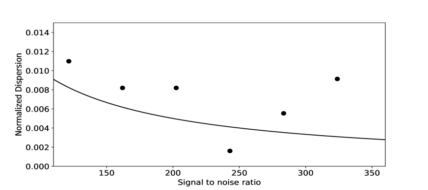
Figure 7: The normalized standard deviation (in percent) of WFC3-IR photometric measurements of GD153 plotted versus the signal to noise ratio. The solid line represents the expected normalized standard deviation ($1/S/N$).

In order to calculate the sensitivity changes over time we performed a first least-square linear fit by including all the measurements of the five standard stars. In the case of the UV filters, we performed two different fits, one for $MJD\leq$ 55738 and a second for all data acquired through $MJD\approx$ 58800, to take into account the change from an increase to a decrease of the sensitivity. We then performed a 2.5 $\sigma$-clipping of the outlier measurements and a second least-square fit that resulted in the final slope values. These are indicated as sensitivity change rates (%/year) in Figs. 1, 2, 3, 4. The final slope values with their uncertainties for UVIS1 and UVIS2 are listed in Table 4 and are plotted as a function of the filter pivot wavelength in Figs.5 and 6.

It is worth noticing that errors on the slopes for some filters are quite large, in particular for the UV filters in the first two years of observations (i.e. when the UV sensitivity change rate was positive). Moreover, uncertainties are larger for a few narrow-, medium-band or long-pass filters, where a limited number ($<$ 20) of standard star measurements were available. In some cases, there were not enough measurements available to calculate a reliable slope. Therefore, we assumed that the sensitivity change rates for these filters were the same as those derived for filters similar in wavelength, but with a much larger data sample. For instance, the slope for filter $F373N$ (pivot wavelength 3730Å) was assumed to be the same as for $F390M$ (pivot wavelength 3897Å, see Table 4).

Table 5: The normalized standard deviation of the WFC3-IR photometric measurements of the standard stars, in percent. The entries labeled with ”*” have less than three data points, and should not be considered as meaningful.

Filter	GD153	GD71	P330E	GRW70	G191B2B
F098M	0.99	1.69	1.07	1.17	1.76
F105W	1.84	1.92	1.16	1.19	1.41
F110W	0.96	1.2	1.01	0.63	1.31
F125W	1.14	1.16	1.03	1.58	0.72
F126N	1.95	0.91	1.05	0.65	0.22*
F127M	1.19	1.03	0.98	0.83	1.36
F128N	1.77	0.94	1.26	0.59	0.1*
F130N	2.3	0.84	1.16	0.39	0.13
F132N	2.49	0.96	1.19	0.29	0.01*
F139M	1.69	0.93	1.0	0.99	0.99
F140W	0.94	1.22	0.88	0.72	0.89
F153M	1.59	0.75	0.71	0.6	0.72
F160W	0.85	0.96	0.92	0.72	0.71
F164N	2.13	1.13	1.14	0.47	0.18*
F167N	2.04	1.04	1.07	0.63	0.05*

Once all the slopes were finalized, we used them to normalize the 10-pixel radius aperture photometry for each standard star and filter to the reference epoch $MJD=$ 55008 (June 26, 2009), corresponding to the time at which the first WFC3 observations were collected. A weighted mean of all measurements was then calculated after a 2.5 $\sigma$-clipping of the outliers. This mean was used to define the value of the photometry at 10 pixels in units of $e^{-}/s$, i.e. in count rates, for each standard star and filter at the reference epoch.

The slopes were then used to derive inverse sensitivities at six different $MJD$ values spaced by 2 years, namely 55008, 56468, 57198, 57928, 58658, 559388, for each filter. calwf3 pipeline then calculates inverse sensitivities at any observing epoch by interpolating over the six provided values (more details are in the following sections). Therefore, the fact that the two least-square fit lines in the case of the $F218W$ filter (Figs.1 and 2), for example, do not perfectly coincide at the established inversion epoch, $MJD=$ 55738, does not affect calwf3 inverse sensitivity calculation.

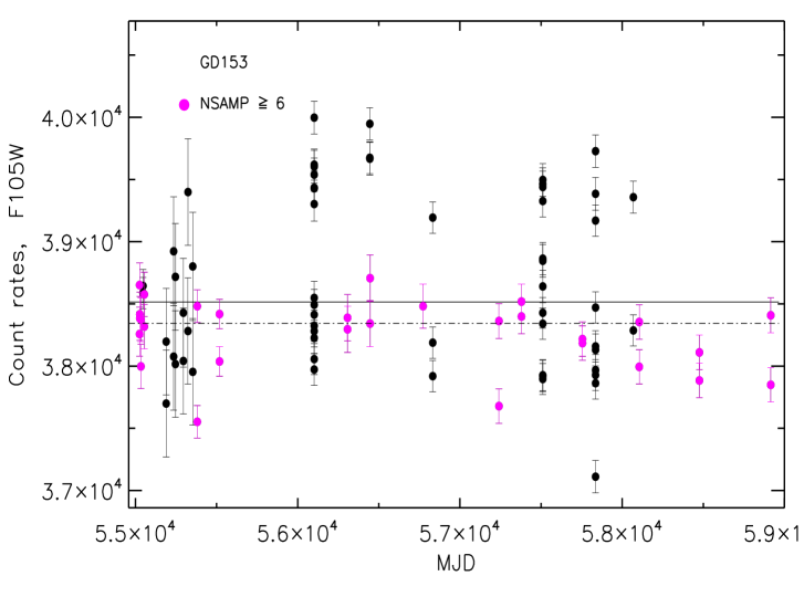
Figure 8: GD153 count rates for the WFC3-IR $F105W$ filter are shown with black filled circles, while measurements from exposures collected with a number of samples (NSAMP) greater than six are marked with magenta filled circles. Error bars are also shown. The solid line indicates the mean of all measurements, while the dotted-dashed line indicates the mean of the NSAMP$\geq$ 6 measurements.

3.2 WFC3-IR

In order to investigate the repeatability of WFC3-IR photometry and to look for possible systematics affecting it, we calculated the 3-$\sigma$ clipped standard deviation of the flux measurements of the five standard stars in each filter normalized by the median flux measurement. This normalized standard deviation is presented in percent and listed in Table 5: while the percent deviation is $\gtrsim$ 1% for most filters, the $S/N$ of many observations is often substantially larger than 100, even including noise imparted from calibration (as reported in the error array of the _flt images). Fig. 7 shows how the dispersion of photometry evolves with the $S/N$ of the exposures: notably, the actual standard deviations are consistently higher than predicted for all $S/N$ levels.

A factor differentiating this analysis from Kalirai et al. (2011) is the usage of updated flat fields (Mack et al., 2021). However, by using the new flat fields the scatter of the standard star measurements was not substantially reduced. This may be partially due to the clustering of the standard star observations near the center of the detector, as the WFC3-IR sub-arrays are all centered. The flat-field error in the center of the detector was already below the half percent level (Dahlen, 2013), and thus the improvement in the new flat fields pixel to pixel variation was minimal.

In some cases, the inclusion of images collected with different observing strategies imparted a higher dispersion on the photometry. Several observations of GD153 in the $F105W$ filter, for example, were collected for the WFC3-IR grism calibration and only included a small number of reads (NSAMP) per exposure; this resulted in noisier data, possibly due to the behavior of the first read of the WFC3-IR integrations (see Fig. 8). Removing low sample exposures from the analysis increased the precision of the photometry for a small subset of the filters, though not to the level predicted by the $S/N$. For instance, the GD153 $F105W$ filter images with less than six reads (NSAMP $\leq$ 6) have a clipped standard deviation of $\approx$ 2%, while those with more reads had a much smaller dispersion, i.e. $\approx$ 0.7%. In addition, the difference between the means of the two populations is $\approx$ 1.3% (Fig. 8). However, removing images collected with less than six reads did not always yield a more precise result; for some stars and filter combinations the dispersion of the measurements increased. The WFC3 team is currently working at better understanding this issue.

The WFC3-IR detector is also affected by persistence, i.e. the residual signal of a large incident light level that can last on the images from minutes to days (Long et al., 2011, 2013; Gennaro et al., 2018). As noted in Bajaj (2019), the effects of persistence significantly lower the precision of WFC3-IR observations. This is likely due to the dependence of persistence signals on time from the stimulus (the exposures that caused the persistence), and fluence of the previous exposures causing the persistence. Additionally, longer term persistence (from observations up to days before) can sometimes still affect the standard star observations (Ryan & Baggett, 2015), though this effect is generally smaller than the self-persistence (persistence from observations in the same visit). The excess flux from persistence is thus not well constrained, and it is virtually indistinguishable from the real flux. The variability of persistence is one of the causes of the lower than expected precision of WFC3-IR observations. Because the effects of persistence on precision photometry were not initially well understood, many of the earlier observations of the standard stars dithered infrequently, and sometimes only by a few pixels. While this may maximize observational efficiency, it incurred a loss of precision. Frequent and large dithers can mitigate much of the effect of the persistence and lead to substantially better precision, and are therefore used in photometric calibration programs since 2017 (Bajaj, 2019).

However, the WFC3-IR detector also exhibits longer term behaviors, where even the first observations in a visit (which should be unaffected by persistence) show photometric offsets compared to previous visits (Bajaj, 2019). In some cases, these offsets are present across a visit. The visit-to-visit variation is distinct from the Poisson error, as Poisson errors manifest randomly. This effect is also detected in WFC3-IR spatial scan data, where Poisson noise terms are effectively close to zero (Som et al., 2021).

A portion of the non-repeatability of the WFC3-IR detector may be then attributed to varying observation configurations (e.g. different sample sequences, number of samples, and exposure time). A substantial detection or correction of systematic behavior as a function of these observation characteristics would likely require additional, extensive processing in the calibration pipelines. This instability between visits is not currently well-understood and the WFC3 team will further investige this issue.

As shown in Fig. 8, standard star data collected over a baseline longer than 10 years do not support a change of sensitivity of the WFC3-IR detector with time. The overall stability of the detector appears to remain similar to the results found in Kalirai et al. (2011) and Bajaj (2019), with a typical dispersion of $\approx$ 1% and no significant consistent trends. However, the lack of precision and the non-repeatability of the photometric measurements might ultimately limit the ability to detect small sensitivity losses (BA20). Specifically, the visit-to-visit variation of the photometry substantially reduces the precision of any time-dependent measurement of the sensitivity. Thus, the standard star measurements are unable to support the findings seen in other studies, such as Kozhurina-Platais & Baggett (2020) and Bohlin et al. (2019). The first analysis detected sensitivity losses of the order of 2% over 10 years for the $F160W$ filter by using observations of the core of the globular cluster $\omega$ Cen; the second analysis found sensitivity losses of $\approx$ 0.17 and 0.08 %/yr for the $G102$ abd $G141$ grism, respectively, by using observations of the four CALSPEC standard WDs. The WFC3 team currently has a calibration program to measure WFC3-IR sensitivity losses via spatial scanning, since this observation strategy allows for extremely small Poisson noise terms. However, preliminary analysis showed uncertainties much larger than the Poisson noise would predict within a visit, and from visit to visit (Som et al., 2021). This effect is not persistence related but appears consistent with the visit-to-visit variability of the standard star measurements. Another technique currently used tby the WFC3 team to verify for WFC3-IR sensitivity losses is observing globular clusters in regions farther away from the core where stellar crowding is less of a concern. A consistent observing strategy between epochs is used in these calibration programs, and should yield more precise measurements of sensitivity losses.

Since no time-dependent correction was applied to the photometry, we calculated a weighted mean of all measurements after a 1.0 $\sigma$-clipping of the outliers for each standard star and filter. The mean was used to define the value of the photometry for each standard star and filter at 3 pixels in units of $e^{-}/s$, i.e. in count rates, at the reference epoch, $MJD=$ 55008 (June 26, 2009).

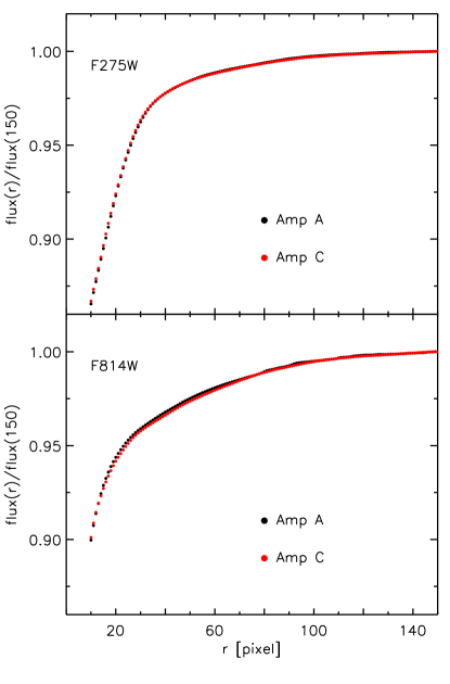
Figure 9: Encircled energy fraction, $flux(r)/flux(150)$, as a function of the aperture radius in pixels, $r$, for Amp A (UVIS1, black filled circles) and Amp C (UVIS2, red) for the $F275W$ (top panel) and the $F814W$ filter (bottom). Photometry was measured on the combined _drc images for the standard star GRW70. See text for more details.

4 Encircled energy corrections

To calculate new inverse sensitivities at infinity, the radius enclosing all of the light emitted by a point source, we first needed to apply encircled energy (EE) corrections (or fractions) to the standard star photometry computed using an aperture radius of 10 pixels for WFC3-UVIS and 3 pixels for WFC3-IR. Uncertainties in the EE corrections are carried over to the uncertainties in the inverse sensitivities. Therefore, in the case of WFC3-UVIS, we applied the new sensitivity change slopes to improve the EE corrections for a subset of filters. For WFC3-IR, new EE corrections were not calculated since the sensitivity changes with time are not well characterized yet for this detector. Instead, the EE solutions from Hartig (2009b) were used to correct the standard star photometry from a 3 pixel radius aperture to infinity.

For WFC3-UVIS, the derived slopes were used to correct the science arrays of the standard star _flc images prior to combining them with AstroDrizzle, and we used this new procedure to recompute EE curves for the $F275W$ and $F814W$ filters. $F275W$ was selected because the EE values in the DE16 (and DE17) solutions differ by $\approx$ 1% from the original in-flight EE calculation by Hartig (2009a) for both UVIS1 and UVIS2. $F814W$ was selected because the EE correction for UVIS2 in the DE16 solution differs from UVIS1 by $\approx$ 0.5% or more for the reddest filters (Hartig, 2009a, see Fig. 10).

Table 6: AstroDrizzle parameters with non-default settings used for this analysis.

Name	Description	Value
skymethod	Equalize sky background between the input frames	match
skystat	Use the sigma-clipped mean background	mean
driz_sep_bits	For single images, set DQ values considered to be good data	64, 16
combine_type	Combine images using the median	median
combine_nhigh	Set the number of high value pixels to reject for the median	1
driz_cr_snr	$S/N$ to be used in detecting CRs, performed in two iterations	3.5 3.0
driz_cr_scale	Scaling factors applied to the derivative for detecting CRs	2.0 1.5
final_bits	For the final stack, set DQ values considered to be good data	64, 16

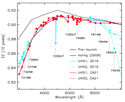
Figure 10: Old (DE16, cyan) and new (CA21, red) EE corrections for UVIS1 (solid line) and UVIS2 (dashed line), as a function of wavelength. The EE model values from Hartig (2009a) are shown with a blue solid line and the pre-launch values with a black solid line.

EE corrections for these two filters were calculated using all in-flight observations collected for the standard star GRW70 from the reference epoch ($MJD$ = 55008) until about $MJD$ = 58800. In particular, each _flc image was multiplied by an inverse sensitivity ratio, i.e. the time-dependent inverse sensitivity value for each image divided by the value at the reference epoch. This was performed using the task phot_eq, which scales the _flc science array values by their respective inverse sensitivity ratio. In this way, all _flc images were corrected to have approximately equal count rates, in preparation for combining the individual frames.

The flux scaled _flc images were then processed using Astrodrizzle to create the combined _ drc image that is used for the EE fraction calculation. The _drc images were produced by combining many individual _flc images, significantly improving the $S/N$ of the standard star and reducing the overall noise, thus enhancing the visibility of the PSF wings. This is very important to achieve more precise photometric measurements at larger aperture radii. For $F275W$, the Amp A (UVIS1) drizzled image was derived from 229 _flc images with a total exposure time of 1,012 seconds, while the Amp C (UVIS2) drizzled image was derived from 185 _flc images, totalling 939 seconds. For $F814W$, the Amp A drizzled image was derived from 117 _flc images, with a total exposure time of 497 seconds, while the Amp C drizzled image was derived from 134 _flc images, totalling 736 seconds.

Whereas the Astrodrizzle algorithm uses pointing information from the _flc image header to align images on the sky, we devised a new approach to align the images in detector coordinates. This ensured that the drizzled PSF did not rotate as the nominal HST orientation varied over the years, which would change the position of the diffraction spikes and structures in the PSF wings. We achieved this by modifying the following astrometry header keywords in each _flc image before drizzling:

• CRPIX1 and CRPIX2 were modified to match the $X,Y$ position of the centroid of the standard star in each image;

• CRVAL1 and CRVAL2 were set to match that of the reference image in order to remove any proper motion applied to the RA and DEC of the standard star over the 10 years;

• The linear terms of the CD matrix (CD1_1, CD1_2, CD2_1, CD2_2) were set to the value in the reference image in order remove any orientation and plate scale changes with date.

Once the astrometry header keywords were updated, we combined the _flc images for each detector using the AstroDrizzle parameter values listed in Table 6. By aligning each star in detector coordinates, we were able to accurately flag and reject artifacts such as cosmic rays and unstable hot pixels, while not affecting any PSF structure. Additionally, by not rotating the images on the sky, the _flc frames have minimal pixel resampling.

Photometry was performed on the _drc images for both filters using aperture radii in the range 1 – 150 (infinity) pixels. The sky value used for background subtraction was computed as the 3-$\sigma$ clipped mean value in an annulus with radii ranging from 160 – 200 pixels. The EE correction for each filter was then estimated as the ratio of the flux (in units of $e^{-}$/s) at different aperture radii and the flux at infinity, defined at a radius of 150 pixels ($\approx$ 6″) for WFC3-UVIS.

After accounting for changes in sensitivity, we find improved agreement in the EE correction values for UVIS1 and UVIS2. For $F275W$ the fraction of flux included in a 10-pixel aperture radius is 86.5$\pm$0.1% for UVIS1 and 86.6$\pm$0.1% for UVIS2, as shown in the top panel of Fig. 9. This differs by $\approx$ 1% from the EE corrections from DE16 which were 87.2% and 87.6% for UVIS1 and UVIS2. Following the results for the F275W filter, we corrected the EE fractions for the other UV filters, namely $F218W$, $F225W$, and $F280N$, scaling them by the difference between the new and old $F275W$ values (see solid and dashed red lines and the marked filter names in Fig. 10). For $F814W$, the new EE fraction is 90.2$\pm$0.1% for UVIS1 and 90.2$\pm$0.1% for UVIS2, as shown in the bottom panel of Fig. 9. The value for UVIS1 agrees with the previous DE16 value of 90.3% to within the measurement uncertainty, while the value for UVIS2 differs by $\approx$ 0.5% with the DE16 value of 90.7%. The new EE corrections for both F275W and F814W agree very well with the values derived from the 2009 optical model (Hartig, 2009a, see Fig. 10).

For filters with pivot wavelengths longer than $F814W$, namely $F845M$, $F850LP$ and $F953N$ (also marked in Fig. 10), we assumed the same EE correction value as derived for the $F814W$ filter. For $F775W$, the DE16 EE values for UVIS2 were $\approx$ 0.5% larger than for UVIS1, so we adopted the UVIS1 values for both detectors. The DE16 EE fractions for a few long-pass and narrow-band filters (marked in the figure) are in large disagreement with the 2009 model values; therefore, we used interpolated EE fractions for these filters based on the values for the two filters closest in wavelength (see Fig. 10).

New aperture correction files, wfc3uvis1_aper_007_syn.fits and wfc3uvis2_aper_007_syn.fits, were created for use in STsynphot and are shown as solid and dashed red lines in Fig. 10. For comparison the DE16 aperture correction files, wfc3uvis1_aper_005_syn.fits and wfc3uvis2_aper_005_syn.fits, are shown as solid and dashed cyan lines. The 2009 EE model values, wfc3_uvis_aper_002_syn.fits, are shown as a solid blue line, while the pre-launch EE values, wfc3_uvis_aper_001_syn.fits, are shown as a solid black line. It is worth noting how well the new UVIS1 and UVIS2 aperture correction files agree with one another and with the model values from (Hartig, 2009a).

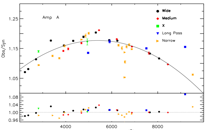
Figure 11: Top - Observed over synthetic count rates for the 42 UVIS1 (Amp A) full-frame filters: wide (black), medium (red), X (green), long Pass (blue), and narrow (orange). These were calculated as a weighted mean over the standard stars. Error bars are displayed. The solid black line is a quadratic polynomial least-square fit to the data of the wide, medium and X filters only. Bottom - The residual ratios after the polynomial fit are shown. The dotted line shows a residual ratio of 1.0 (see text for more details).

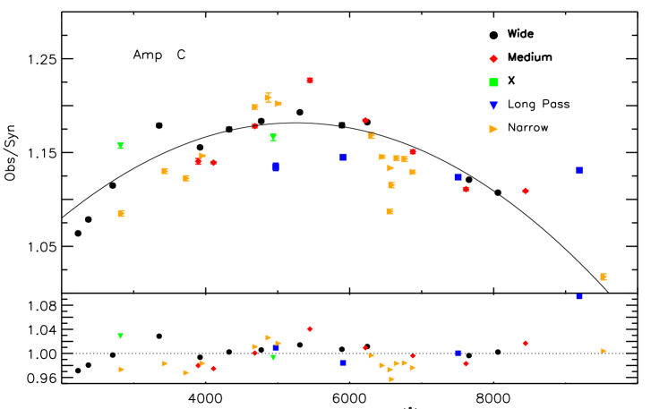
Figure 12: Same as Fig. 11 but for the 42 UVIS2 (Amp C) full-frame filters.

5 New in-flight corrections and filter curves

We used the new EE fractions to correct WFC3-UVIS standard star photometry from a 10 pixel aperture radius to infinity. We obtained mean count rates for each standard star as observed with the two detectors through all the 42 full-frame filters at the reference epoch $MJD=$ 55008.

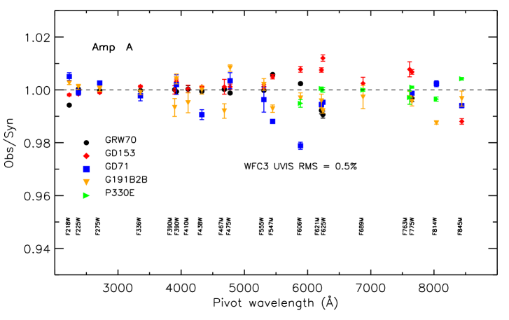
Figure 13: Observed over synthetic count rates for UVIS1 (Amp A) wide- and medium-band filters for the five standard stars used in the calibration as a function of the pivot wavelength. Error bars are displayed. Note that ratios for P330E were calculated for $\lambda>$ 6000Å  only.

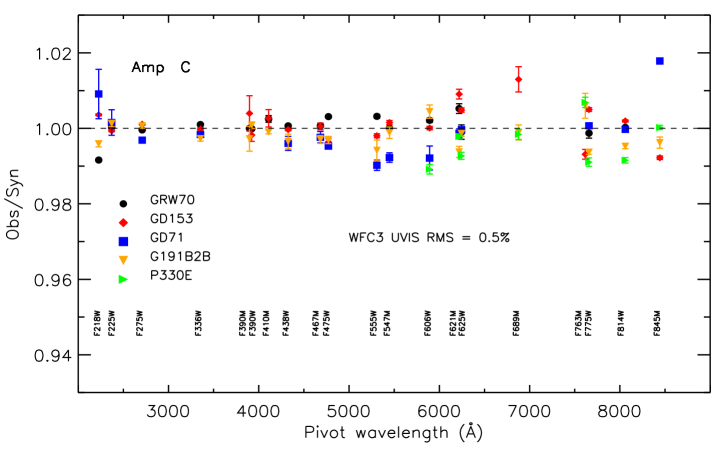
Figure 14: Same as Fig. 13 but for UVIS2 (Amp C) filters.

Table 7: Files used in the synthetic simulations performed with Pysynphot.

Component	Description
Simulations to derive the new in-flight corrections for WFC3-UVIS
wfc3_uvis_cor_003_syn.fits	Original in-flight correction, all entries set to 1.0
wfc3uvis1_aper_007_syn.fits	New aperture correction for UVIS1
wfc3uvis2_aper_007_syn.fits	New aperture correction for UVIS2
wfc3_uvis_FXXXX_002/003_syn.fits	Pre-launch filter curves (TV3)
gd153_stiswfcnic_002.fits	New CALSPEC SED
gd71_stiswfcnic_002.fits	New CALSPEC SED
gd191b2b_stiswfcnic_002.fits	New CALSPEC SED
grw_70d5824_stiswfcnic_002.fits	New CALSPEC SED
p330e_stiswfcnic_002.fits	New CALSPEC SED
Simulations to derive the new filter curves for WFC3-UVIS
wfc3uvis1_cor_005_syn.fits	New in-flight correction for UVIS1
wfc3uvis2_cor_005_syn.fits	New in-flight correction for UVIS2
wfc3uvis1_aper_007_syn.fits	New aperture correction for UVIS1
wfc3uvis2_aper_007_syn.fits	New aperture correction for UVIS2
wfc3_uvis_FXXXX_002/003_syn.fits	Pre-launch filter curves (TV3)
gd153_stiswfcnic_002.fits	New CALSPEC SED
gd71_stiswfcnic_002.fits	New CALSPEC SED
gd191b2b_stiswfcnic_002.fits	New CALSPEC SED
grw_70d5824_stiswfcnic_002.fits	New CALSPEC SED
p330e_stiswfcnic_002.fits	New CALSPEC SED
Simulations to derive the final synthetic count rates for WFC3-UVIS
wfc3uvis1_cor_005_syn.fits	New in-flight correction for UVIS1
wfc3uvis2_cor_005_syn.fits	New in-flight correction for UVIS2
wfc3uvis1_aper_007_syn.fits	New aperture correction for UVIS1
wfc3uvis2_aper_007_syn.fits	New aperture correction for UVIS2
wfc3uvis1_FXXXX_008_syn.fits	New filter curves for UVIS1
wfc3uvis2_FXXXX_008_syn.fits	New filter curves for UVIS2
gd153_stiswfcnic_002.fits	New CALSPEC SED
gd71_stiswfcnic_002.fits	New CALSPEC SED
gd191b2b_stiswfcnic_002.fits	New CALSPEC SED
grw_70d5824_stiswfcnic_002.fits	New CALSPEC SED
p330e_stiswfcnic_002.fits	New CALSPEC SED
Simulations to derive the new filter curves for WFC3-IR
wfc3_ir_cor_004_syn.fits	Original in-flight correction
wfc3_ir_aper_002_syn.fits	Original aperture correction
wfc3_ir_FXXXX_004/005_syn.fits	2012 filter curves
gd153_stiswfcnic_002.fits	New CALSPEC SED
gd71_stiswfcnic_002.fits	New CALSPEC SED
gd191b2b_stiswfcnic_002.fits	New CALSPEC SED
grw_70d5824_stiswfcnic_002.fits	New CALSPEC SED
p330e_stiswfcnic_002.fits	New CALSPEC SED
Simulations to derive the final synthetic count rates for WFC3-IR
wfc3_ir_cor_004_syn.fits	Original in-flight correction
wfc3_ir_aper_002_syn.fits	Original aperture correction
wfc3_ir_FXXXX_007_syn.fits	New filter curves
gd153_stiswfcnic_002.fits	New CALSPEC SED
gd71_stiswfcnic_002.fits	New CALSPEC SED
gd191b2b_stiswfcnic_002.fits	New CALSPEC SED
grw_70d5824_stiswfcnic_002.fits	New CALSPEC SED
p330e_stiswfcnic_002.fits	New CALSPEC SED

WFC3-UVIS filter curves were first calculated during three thermal vacuum (TV) tests performed at NASA Goddard by using the CASTLE apparatus. This system illuminated the detector with a monochromatic flux source and aperture photometry was derived on the images. The filter curves resulting from the third test, TV3, were delivered and presented in Brown (2008). These curves were updated after WFC3 was installed on HST, and the first in-flight correction and inverse sensitivities were derived by Kalirai et al. (2009b).

Different in-flight corrections for UVIS1 and UVIS2 were later delivered by DE16, when WFC3 chips were independently calibrated.

In order to update the in-flight corrections and derive new filter curves we used Pysynphot (Lim et al. 2015) to predict the count rates for each filter and standard star as observed with UVIS1 and UVIS2 at the reference epoch. As input for the Pysynphot simulations, we used no in-flight correction (the wfc3_uvis_cor_003_syn.fits file has all entries set to 1.0), the filter curves from TV3 (wfc3_uvis_FXXX_002/003_syn.fits), and the new aperture correction files we calculated (wfc3uvis1/2_aper_007_syn.fits), all listed in Table 7. The simulations also used other components, such as the HST Optical Telescope Assembly (OTA), the pick-off mirror, the mirrors’ reflectivity, the inner and outer window, and the quantum efficiency (QE) of each detector.

We also used new SEDs of the three HST primary WDs provided by the CALSPEC database (_stiswfcnic_002); these were calculated with the Non-Local Thermal-Equilibrium (NLTE) code from TMAP (Rauch et al., 2013) and TLUSTY (Hubeny, 2017). The models were normalized to an absolute flux level defined by the flux of 3.47$\times$10^-9 erg cm^-2 s^-1 Å^-1 for Vega at 0.5556$\mu$m, as reconciled with the MSX mid-IR absolute flux measures (for more details please see BO20). We used new SEDs for GRW70 and P330E as well, as delivered in the CALSPEC database by BO20 and listed in the same table.

We then derived the ratio of observed over synthetic count rates for each star, detector and filter: in the case of UV and bluer filters, i.e. for wavelengths $\lambda<$ 6000Å, we calculated a weighted mean of the ratios by using the four standard WDs, while for longer wavelengths we used all five stars in the calculations, i.e. we also included the G-type star P330E, when measurements were available. We followed this strategy since photometric measurements for P330E have a much lower $S/N$ in the bluer filters and a significant color term ($\approx$ 1 to 8%) is present when observing red sources with UV filters, i.e. the response of the detector and filter for red stars is different compared to the response for blue stars (CA18). Figs. 11 and 12 show the ratios of observed over synthetic count rates for all filters and Amp A (UVIS1) and Amp C (UVIS2), respectively. The ratio values for all filters are larger than 1.0, i.e. the throughputs were underestimated before WFC3 launch. A very similar result was found by Kalirai et al. (2009b, see their Fig. 5) and DE16 (see their Fig. 8) based on observations collected in 2009 and 6 years of standard star photometry, respectively. The pre-launch throughput values were measured during the TV3 campaign and were systematically underestimated, on average by 5–10% and up to 20% for wavelengths around $\lambda\sim$ 5000Å. A possible explanation provided by Kalirai et al. is that the TV3 calibration error was due to problems with the CASTLE apparatus (see also Brown 2008).

The residuals of the observed over synthetic ratios after applying the new in-flight corrections are larger for the narrow-band filters (see bottom panel in Figs. 11 and 12), as expected, due to the availability of many less standard star measurements in these filters compared to the others, the lower $S/N$, and in some cases the presence of absorption lines. For example, the ratio and the residual for the $F656N$ filter are systematically lower (by $\approx$ 10 and 5%) compared to the other filters, probably due to the presence of a $H_{\alpha}$ line in the standard WD SEDs.

The long-pass filters also show slightly larger residuals due to few measurements available. Therefore, we only used the wide-, medium-band and the extremely-wide (X) filters to derive the new in-flight corrections.

A least-square fit with a quadratic polynomial (Amp A: $0.93+9\cdot 10^{-5}\cdot\lambda-8\cdot 10^{-9}\cdot\lambda^{2}$, Amp C: $0.92+1\cdot 10^{-4}\cdot\lambda-1\cdot 10^{-8}\cdot\lambda^{2}$, where the wavelength is in units of Å) resulted the best method to reproduce the data points and it is shown with a solid line in Figs. 11 and 12. The bottom panel of the figures shows the residual ratios for each filter after the fit. The ratios between observed and synthetic count rates have a mean value of 1.00 with a dispersion $\approx$ 0.02.

We then created a new in-flight correction file for each detector, wfc3uvis1_cor_005_syn.fits and wfc3uvis2_cor_005_syn.fits, by using the derived polynomials (Table 7). New synthetic count rates were thus calculated with the new in-flight corrections and the same SEDs, filter curves and aperture corrections. The ratio of observed and new synthetic count rates was used to derive a multiplicative scalar correction to be applied to each filter curve. New filter curves were created, and named as wfc3uvis1_FXXXX_008_syn.fits and wfc3uvis2_FXXXX_008_syn.fits, and used to calculate the final synthetic count rates for each detector, filter and standard star. These new filter curves provided count rates as observed at the reference epoch. Time-dependent filter curves were also created, wfc3uvis1_FXXXX_mjd_008_syn.fits and wfc3uvis2_FXXXX_mjd_008_syn.fits, by using the sensitivity change rates and calculating the filter curve for six different epochs spaced by two years each. The wfc3uvis1,2_FXXXX_mjd_008_syn.fits files thus have seven different throughput columns, one for the reference epoch and other six for different increasing $MJD$ values, until $MJD$ = 59388 (June 23, 2021).

To generate synthetic count rates for any star and any filter as measured by WFC3-UVIS at different epochs ($MJDs$), Pysynphot or the more recently delivered STsynphot(STScI Development Team, 2018), interpolate between two of the six consecutive $MJD$ values included in the filter curve tables. If the requested epoch is outside the current lifetime of WFC3, the values will be extrapolated in the future or in the past. However, the extrapolation to $MJD$ values before the reference epoch, i.e. before WFC3 was launched, is not reliable and should not be used in simulations.

Figs. 13 and  14 show the observed over synthetic count rates for the five standard stars and the wide- and medium-band filters obtained by using the new filter curves in the Pysynphot simulations. The ratio values cluster around 1.0, as expected, with a RMS of 0.5% for both detectors and including all filters.

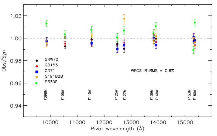
Figure 15: Observed over synthetic count rates for WFC3 IR wide- and medium-band filters for the five standard stars used in the calibration as a function of the pivot wavelength.

In the case of WFC3-IR, we performed Pysynphot simulations by using the new standard star SEDs, the original in-flight correction (004) from Kalirai et al. (2009a), the 2012 filter curves (004/005), and the original aperture correction (002), as listed in Table 7. We also used all the other components, such as the HST OTA, the pick-off mirror, the mirror reflectivity, the inner and outer window, and the QE for the WFC3-IR detector.

We thus derived the ratio of observed over synthetic count rates for each standard star and filter and calculated a weighted mean of the ratios by using the four WDs and the G-type star P330E. The ratio of observed and new synthetic count rates was then used to derive a multiplicative scalar correction to be applied to each filter curve. New filter curves were created, and named as wfc3_ir_FXXXX_007_syn.fits, and used to calculate the final synthetic count rates for each filter and standard star. These new filter curves provided count rates as observed at the same reference epoch as WFC3-UVIS, i.e. $MJD$ = 55008. Filter curves including the same time-dependent columns ($MJD$) as the WFC3-UVIS filter curves were also created, wfc3_ir_FXXXX_mjd_007_syn.fits; however, no time dependence was introduced for WFC-IR inverse sensitivities and the different $MJD$ columns all contain the same values. Fig. 15 shows the observed over synthetic count rates for the five standard stars and the wide- and medium-band filters obtained with the new WFC3-IR filter curves. The ratio values cluster around 1.0, as expected, with a RMS of 0.6%, including all filters.

5.1 Quad filters

The quad filters are made of a 2$\times$2 mosaic of elements occupying a single filter slot, with each quadrant providing a different bandpass; therefore, the five quad filter sets generate 20 different narrow- and medium-band filters. The readout amplifier for each quad filter is listed in Table 9.

In the case of the quad filters, only the standards GD153, G191B2B and P330E were observed and not enough measurements were collected to determine slopes for the sensitivity changes with time. Therefore, we used the available photometry to calculate the weighted mean count rates for each standard star in each filter and assumed the same reference epoch as for the other WFC3-UVIS filters, i.e. $MJD$ = 55008.

Synthetic count rates were calculated by using the new SEDs for the standard stars and the original in-flight correction (wfc3_uvis_cor_003_syn.fits), the original aperture correction file (wfc3_uvis_aper_002_syn.fits), and the original filter curves (wfc3_uvis_FQXXX_004_syn.fits or wfc3_uvis_FQXXX_005_syn.fits). We then obtained a weighted mean of the ratios by using the two WDs and the G-type star P330E and derived multiplicative scalar factors to create new filter curves. These are named as wfc3_uvis_FQXXXX_008_syn.fits or wfc3uvis2_FQXXXX_mjd_008_syn.fits. As in the case of WFC3-IR, no time dependence is included in the quad filter curves, and the different $MJD$ columns have all the same throughput values. It is worth noting that only one in-flight, one aperture correction and one filter curve file, named as _uvis, is available for the quad filters, irregardless of the quadrant (amplifier) in which the filters fall.

6 Calculating the inverse sensitivities

Updated synthetic count rates and photometry for the five standard stars for both WFC3-UVIS and IR were used to derive new inverse sensitivities. We followed the method presented in Bohlin et al. (2014, 2020) and DE16. The point source mean flux over a passband can be defined in wavelength units, $erg$ $s^{-1}$ $cm^{-2}$ Å^-1, as:

$$<F_{\lambda}>=\frac{\int F_{\lambda}\cdot\lambda\cdot R\cdot d\lambda}{\int\lambda\cdot R\cdot d\lambda}=S_{\lambda}\cdot N_{e}$$ (1)

or in frequency units, $erg$ $s^{-1}$ $cm^{-2}$ $Hz^{-1}$, as:

$$<F_{\nu}>=\frac{\int F_{\nu}\cdot\nu\cdot R\cdot d\nu}{\int\nu\cdot R\cdot d\nu}=S_{\nu}\cdot N_{e}$$ (2)

where $R$ is the system throughput, $S_{\lambda}$ and $S_{\nu}$ are the instrument sensitivities, $N_{e}$ is the instrumental count rate in $e^{-}/s$, and the integrals are calculated over the passband (Koornneef et al., 1986; Rieke et al., 2008).

The detector count rate, $N_{e}$, can be measured or calculated as:

$$N_{e}=\frac{A}{hc}\int F_{\lambda}\cdot\lambda\cdot R\cdot d\lambda=A\int\frac{F_{\nu}}{h\nu}\cdot R\cdot d\nu$$ (3)

where $A$ is the telescope collecting area, $h$ is the Planck constant, $c$ is the speed of light.

The instrument sensitivities $S$ are then defined by dividing the mean flux of Eqs. (1) and (2) by the detected count rate, $N_{e}$, and are expressed in units of $erg$ $cm^{-2}$ Å^-1 $e^{-1}$:

$$S_{\lambda}=\frac{<F_{\lambda}>}{N_{e}}=\frac{hc}{A\cdot\int\lambda\cdot R\cdot d\lambda}$$ (4)

or $erg$ $cm^{-2}$ $Hz^{-1}$ $e^{-1}$:

$$S_{\nu}=\frac{<F_{\nu}>}{N_{e}}=\frac{h}{A\cdot\int\nu^{-1}\cdot R\cdot d\nu}$$ (5)

We refer to $S$ as the ’inverse sensitivity’ since a more sensitive detector will have larger count rates, $N_{e}$, for the same source flux $F_{\lambda}$ or $F_{\nu}$.

$S_{\lambda}$ at infinity is provided in the image header for UVIS1 and UVIS2 as the PHFTLAM1 and PHTFLAM2 keywords, respectively. The PHOTFLAM keyword is set to the value of PHTFLAM1, except for the UV filters (see below). The ratio of the UVIS2 and UVIS1 inverse sensitivities ($S_{2}/S_{1}$ or PHTFLAM2/PHTFLAM1) is indicated in the image header by the keyword PHTRATIO (see Section 6.1).

In the case of the WFC3-IR detector, $S_{\nu}$ is also provided in the image header as the PHOTFNU keyword.

For observations collected with UV filters, namely $F218W$, $F225W$, $F275W$ and $F200LP$, the value of the UVIS1 inverse sensitivity is modified ($S_{1}^{{}^{\prime}}$), such that the ratio of the inverse sensitivities, PHTRATIO ($S_{2}/S_{1}^{{}^{\prime}}$), is equal to the ratio of the observed count rates, $C_{1}/C_{2}$ (DE17). This tweak is necessary since the response functions of UVIS1 and UVIS2 are significantly different in the UV regime, and WFC3 processing pipeline, calwf3, needs PHTRATIO to flux scale the UVIS2 detector to UVIS1. However, the equivalency of the modified inverse sensitivity ratio, $S_{2}/S_{1}^{{}^{\prime}}$, to the count rate ratio, $C_{1}/C_{2}$, only holds for hot stars, i.e. $T_{eff}\gtrsim$ 30,000K, since cooler stars have a largely different SEDs in the UV, and the response of the detector + filter system is different for these sources. Therefore, magnitude offsets for the UV filters as a function of the source color need be applied to magnitudes measured on UVIS2 to transform the photometry to the UVIS1 photometric system. These corrections are currently available in CA18 (see §9 for more details).

Inverse sensitivities at infinity were also derived for the 15 WFC3-IR filters and indicated in the image header as the PHOTFLAM and PHOTFNU keywords.

The new inverse sensitivities for UVIS1 and UVIS2 at the reference epoch, $MJD=$ 55008 (June 26, 2009), are listed in Tables LABEL:table:8 (42 full-frame filters) and Table 9 (20 quad filters). Table 10 lists the new inverse sensitivities for the 15 WFC3-IR filters at the same reference epoch. Inverse sensitivities are also provided at the WFC3 Photometric Calibration web pages for WFC3-UVIS and WFC3-IR.

Inverse sensitivities can also be computed for any observation epoch by using STsynphot and the new set of filter curves, in-flight and aperture corrections: example tutorials are provided at the same web pages or at the STScI WFC3 Software Library on GitHub.

Table 8: New inverse sensitivity values (PHOTFLAM) and ZPs in different photometric systems for UVIS1 (Amp A) and UVIS2 (Amp C) 42 full-frame filters calculated at the reference epoch $MJD=$ 55008 (June 26, 2009). Errors are also listed.

Filter	Pivot	PHOTBW	ZPAB	ZPVega	ZPST	ZPERR	PHOTFLAM	PHOTFLAMERR
	(Å)	(Å)	(Mag)	(Mag)	(Mag)	(Mag)	(erg cm-2 Å-1 e-1)	(erg cm-2 Å-1 e-1)
UVIS1 (Amp A)
F200LP	4971.86	1742.20	27.3356	26.8857	27.1261	0.0128	5.1234e-20	6.0032e-22
F218W	2228.04	128.94	22.9368	21.2726	20.9843	0.0072	1.4664e-17	9.6609e-20
F225W	2372.05	177.43	24.0631	22.4257	22.2467	0.0015	4.5849e-18	6.2529e-21
F275W	2709.69	164.43	24.1569	22.6759	22.6294	0.0017	3.2227e-18	5.1180e-21
F280N	2832.86	200.69	20.9180	19.5016	19.4871	0.0085	5.8231e-17	4.5543e-19
F300X	2820.47	316.56	24.9638	23.5611	23.5234	0.0024	1.4147e-18	3.1311e-21
F336W	3354.49	158.42	24.6908	23.5260	23.6269	0.0018	1.2860e-18	2.1606e-21
F343N	3435.15	86.71	23.8868	22.7517	22.8745	0.0016	2.5716e-18	3.6774e-21
F350LP	5873.87	1490.06	26.9647	26.8116	27.1173	0.0050	5.1653e-20	2.4005e-22
F373N	3730.17	18.34	21.9076	21.0354	21.0742	0.0090	1.3499e-17	1.1206e-19
F390M	3897.24	65.48	23.6216	23.5457	22.8834	0.0052	2.5506e-18	1.2257e-20
F390W	3923.69	291.27	25.3725	25.1735	24.6489	0.0032	5.0170e-19	1.4587e-21
F395N	3955.19	26.29	22.6678	22.7115	21.9616	0.0024	5.9616e-18	1.3191e-20
F410M	4108.99	57.03	23.5959	23.7699	22.9726	0.0038	2.3495e-18	8.2162e-21
F438W	4326.23	197.31	24.8367	25.0015	24.3252	0.0060	6.7593e-19	3.7819e-21
F467M	4682.58	68.42	23.6935	23.8567	23.3539	0.0062	1.6536e-18	9.5492e-21
F469N	4688.10	19.97	21.8160	21.9825	21.4790	0.0029	9.2985e-18	2.5187e-20
F475W	4773.10	421.30	25.7039	25.8094	25.4058	0.0055	2.4984e-19	1.2504e-21
F475X	4940.72	660.68	26.1558	26.2131	25.9327	0.0017	1.5379e-19	2.3980e-22
F487N	4871.38	21.71	22.2269	22.0479	21.9731	0.0039	5.8987e-18	2.1052e-20
F502N	5009.64	26.96	22.3262	22.4190	22.1332	0.0050	5.0899e-18	2.3595e-20
F547M	5447.50	206.24	24.7550	24.7583	24.7440	0.0100	4.5959e-19	4.2627e-21
F555W	5308.43	517.49	25.8097	25.8379	25.7425	0.0028	1.8324e-19	4.6668e-22
F600LP	7468.12	945.89	25.8820	25.5487	26.5560	0.0070	8.6611e-20	5.5311e-22
F606W	5889.17	657.20	26.0872	26.0039	26.2454	0.0129	1.1529e-19	1.3885e-21
F621M	6218.85	185.65	24.6124	24.4620	24.8889	0.0070	4.0217e-19	2.5967e-21
F625W	6242.56	451.28	25.5247	25.3736	25.8095	0.0094	1.7225e-19	1.4834e-21
F631N	6304.29	41.60	21.8849	21.7232	22.1910	0.0114	4.8259e-18	5.0616e-20
F645N	6453.59	41.45	22.2434	22.0478	22.6004	0.0039	3.3101e-18	1.1955e-20
F656N	6561.37	41.77	20.4221	19.8404	20.8151	0.0385	1.7137e-17	5.9545e-19
F657N	6566.63	41.00	22.6585	22.3324	23.0531	0.0043	2.1815e-18	8.7084e-21
F658N	6584.02	148.71	21.0271	20.6717	21.4275	0.0177	9.7468e-18	1.5697e-19
F665N	6655.88	42.19	22.7339	22.4901	23.1578	0.0096	1.9808e-18	1.7401e-20
F673N	6765.94	41.94	22.5877	22.3424	23.0473	0.0069	2.1931e-18	1.3993e-20
F680N	6877.60	112.01	23.8182	23.5546	24.3133	0.0140	6.8336e-19	8.9134e-21
F689M	6876.75	207.61	24.4777	24.1950	24.9725	0.0028	3.7238e-19	9.6694e-22
F763M	7614.37	229.42	24.2260	23.8366	24.9421	0.0068	3.8296e-19	2.3862e-21
F775W	7651.36	419.72	24.8714	24.4800	25.5981	0.0048	2.0930e-19	9.1984e-22
F814W	8039.06	666.76	25.1272	24.6985	25.9612	0.0075	1.4980e-19	1.0373e-21
F845M	8439.06	260.30	23.8216	23.3150	24.7610	0.0091	4.5246e-19	3.8212e-21
F850LP	9176.13	470.53	23.8557	23.3253	24.9769	0.0066	3.7086e-19	2.2782e-21
F953N	9530.58	71.19	20.4250	19.8019	21.6285	0.0111	8.1018e-18	8.2727e-20
UVIS2 (Amp C)
F200LP	4875.10	1725.22	27.3803	26.9000	27.1282	0.0127	5.1134e-20	5.9509e-22
F218W	2223.72	124.92	23.2115	21.5463	21.2548	0.0106	1.1430e-17	1.1093e-19
F225W	2358.39	173.15	24.2791	22.6377	22.4501	0.0012	3.8015e-18	4.2937e-21
F275W	2703.30	165.58	24.2223	22.7373	22.6897	0.0021	3.0488e-18	5.9952e-21
F280N	2829.98	202.41	20.9303	19.5123	19.4972	0.0182	5.7693e-17	9.5770e-19
F300X	2805.84	316.95	25.0513	23.6394	23.5995	0.0117	1.3186e-18	1.4264e-20
F336W	3354.65	158.34	24.7185	23.5538	23.6547	0.0022	1.2535e-18	2.5211e-21
F343N	3435.19	86.65	23.9236	22.7885	22.9113	0.0042	2.4858e-18	9.6503e-21
F350LP	5851.15	1483.02	26.9356	26.7802	27.0798	0.0048	5.3469e-20	2.3475e-22
F373N	3730.16	18.29	21.9350	21.0628	21.1016	0.0051	1.3163e-17	6.1663e-20
F390M	3897.00	65.47	23.6375	23.5611	22.8992	0.0037	2.5138e-18	8.5689e-21
F390W	3920.72	291.16	25.3811	25.1779	24.6559	0.0017	4.9849e-19	7.8536e-22
F395N	3955.15	26.30	22.6700	22.7139	21.9638	0.0034	5.9495e-18	1.8615e-20
F410M	4108.88	56.96	23.5944	23.7683	22.9709	0.0029	2.3530e-18	6.3673e-21
F438W	4325.14	197.42	24.8343	24.9990	24.3223	0.0034	6.7777e-19	2.1424e-21
F467M	4682.60	68.37	23.6984	23.8616	23.3588	0.0024	1.6461e-18	3.7092e-21
F469N	4688.10	20.07	21.8199	21.9864	21.4828	0.0089	9.2649e-18	7.6216e-20
F475W	4772.17	421.76	25.6961	25.8017	25.3977	0.0048	2.5172e-19	1.1204e-21
F475X	4937.41	661.13	26.1519	26.2092	25.9273	0.0045	1.5455e-19	6.4132e-22
F487N	4871.38	21.84	22.2413	22.0624	21.9875	0.0165	5.8199e-18	8.8914e-20
F502N	5009.63	27.10	22.3215	22.4143	22.1285	0.0048	5.1120e-18	2.2581e-20
F547M	5447.24	206.18	24.7592	24.7625	24.7480	0.0050	4.5792e-19	2.1269e-21
F555W	5307.91	517.13	25.7962	25.8245	25.7288	0.0076	1.8556e-19	1.3004e-21
F600LP	7453.66	937.10	25.8573	25.5254	26.5271	0.0090	8.8952e-20	7.3298e-22
F606W	5887.71	656.93	26.0785	25.9954	26.2361	0.0079	1.1629e-19	8.5554e-22
F621M	6219.16	185.71	24.6065	24.4560	24.8831	0.0068	4.0434e-19	2.5181e-21
F625W	6241.96	451.09	25.5247	25.3736	25.8092	0.0049	1.7231e-19	7.8251e-22
F631N	6304.28	42.39	21.8900	21.7283	22.1961	0.0102	4.8033e-18	4.4718e-20
F645N	6453.58	42.24	22.2381	22.0425	22.5951	0.0050	3.3263e-18	1.5421e-20
F656N	6561.36	42.44	20.4568	19.8751	20.8497	0.0126	1.6600e-17	1.9100e-19
F657N	6566.60	41.07	22.6580	22.3319	23.0527	0.0051	2.1824e-18	1.0186e-20
F658N	6583.92	151.15	21.0376	20.6820	21.4379	0.0080	9.6562e-18	7.1081e-20
F665N	6655.84	42.26	22.7212	22.4775	23.1452	0.0062	2.0041e-18	1.1303e-20
F673N	6765.91	42.13	22.5625	22.3171	23.0220	0.0121	2.2447e-18	2.4847e-20
F680N	6877.41	112.06	23.7974	23.5339	24.2925	0.0065	6.9662e-19	4.1363e-21
F689M	6876.50	207.84	24.4682	24.1855	24.9630	0.0100	3.7566e-19	3.4228e-21
F763M	7612.74	228.87	24.2051	23.8160	24.9208	0.0087	3.9054e-19	3.1189e-21
F775W	7648.30	418.28	24.8610	24.4700	25.5868	0.0067	2.1149e-19	1.3204e-21
F814W	8029.32	663.97	25.1118	24.6841	25.9431	0.0056	1.5232e-19	7.8754e-22
F845M	8437.27	259.71	23.8125	23.3060	24.7515	0.0123	4.5641e-19	5.1436e-21
F850LP	9169.94	466.6	23.8099	23.2799	24.9297	0.0076	3.8736e-19	2.7041e-21
F953N	9530.50	72.85	20.3831	19.7601	21.5866	0.0122	8.4191e-18	9.5450e-20

Table 9: New inverse sensitivity values (PHOTFLAM) and ZPs in different photometric systems for the 20 quad filters calculated at the reference epoch $MJD=$ 55008 (June 26, 2009). Errors are also listed.

Filter	Chip	Pivot	PHOTBW	ZPAB	ZPVega	ZPST	ZPERR	PHOTFLAM	PHOTFLAMERR
		(Å)	(Å)	(Mag)	(Mag)	(Mag)	(Mag)	(erg cm-2 Å-1 e-1)	(erg cm-2 Å-1 e-1)
FQ232N	UVIS2	2432.22	263.50	20.4123	18.8028	18.6502	0.0064	1.2587e-16	7.4676e-19
FQ243N	UVIS2	2476.32	193.97	20.7378	19.1082	19.0148	0.0129	9.0301e-17	9.5288e-18
FQ378N	UVIS1	3792.41	32.14	22.7507	22.2919	21.9532	0.0136	6.0299e-18	3.8173e-19
FQ387N	UVIS1	3873.66	15.01	21.3399	21.2738	20.5884	0.0136	2.0928e-17	2.8522e-19
FQ422M	UVIS2	4219.21	38.33	22.6725	22.9269	22.1066	0.0185	5.1880e-18	5.3523e-20
FQ436N	UVIS2	4367.16	22.82	21.6299	21.6775	21.1389	0.0081	1.2684e-17	3.1092e-19
FQ437N	UVIS1	4371.04	21.60	21.2682	21.3942	20.7790	0.0369	1.7282e-17	5.5396e-19
FQ492N	UVIS1	4933.44	35.18	22.8676	22.9380	22.6413	0.0073	3.1887e-18	1.5797e-20
FQ508N	UVIS1	5091.05	42.37	22.8805	22.9579	22.7225	0.0389	2.9976e-18	1.5032e-19
FQ575N	UVIS2	5757.69	42.20	20.5297	20.4709	20.6388	0.0537	2.0246e-17	7.3602e-19
FQ619N	UVIS1	6198.52	36.45	21.9403	21.7985	22.2097	0.0160	4.7187e-18	6.4863e-20
FQ634N	UVIS2	6349.21	43.00	21.9575	21.7809	22.2790	0.0307	4.4312e-18	7.6042e-20
FQ672N	UVIS2	6716.38	70.00	20.3946	20.1585	20.8382	0.0960	1.5193e-17	1.6124e-18
FQ674N	UVIS1	6730.68	39.20	20.6923	20.4535	21.1406	0.0403	1.6657e-17	6.8407e-18
FQ727N	UVIS2	7275.23	63.22	21.5808	21.2474	22.1979	0.0676	4.7367e-18	2.6141e-19
FQ750N	UVIS1	7502.50	28.12	21.5024	21.1309	22.1864	0.0561	4.6196e-18	2.9526e-19
FQ889N	UVIS1	8892.15	55.49	21.0572	20.5360	22.1102	0.0181	5.0706e-18	5.8733e-19
FQ906N	UVIS2	9057.76	57.30	20.9512	20.4312	22.0443	0.0500	5.3340e-18	2.4683e-19
FQ924N	UVIS2	9247.59	46.28	20.7532	20.1576	21.8913	0.0500	6.3554e-18	2.9059e-18
FQ937N	UVIS1	9372.42	54.80	20.6478	20.1671	21.8150	0.0045	7.2367e-18	4.2433e-19

Table 10: New inverse sensitivity values (PHOTFLAM) and ZPs in different photometric systems for the 15 WFC3-IR filters calculated at the reference epoch $MJD=$ 55008 (June 26, 2009). Errors are also listed.

Filter	Pivot	PHOTBW	ZPAB	ZPVega	ZPST	ZPERR	PHOTFLAM	PHOTFLAMERR
	(Å)	(Å)	(Mag)	(Mag)	(Mag)	(Mag)	(erg cm-2 Å-1 e-1)	(erg cm-2 Å-1 e-1)
F098M	9864.72	500.85	25.6661	25.0900	26.9445	0.0080	6.0653e-20	4.3288e-22
F105W	10551.05	845.62	26.2637	25.6025	27.6882	0.0047	3.0507e-20	1.4230e-22
F110W	11534.46	1428.48	26.8185	26.0418	28.4364	0.0046	1.5318e-20	6.5390e-23
F125W	12486.06	866.28	26.2321	25.3117	28.0221	0.0078	2.2446e-20	1.6252e-22
F126N	12584.89	339.31	22.8491	21.9083	24.6563	0.0079	4.9671e-19	3.6832e-21
F127M	12740.29	249.56	24.6246	23.6432	26.4584	0.0122	9.4524e-20	1.0141e-21
F128N	12831.84	357.44	22.9561	21.8982	24.8055	0.0078	4.3480e-19	2.9263e-21
F130N	13005.68	274.24	22.9813	21.9849	24.8599	0.0081	4.1416e-19	2.5823e-21
F132N	13187.71	319.08	22.9325	21.9145	24.8413	0.0071	4.2096e-19	2.9310e-21
F139M	13837.62	278.02	24.4663	23.3663	26.4796	0.0043	9.3134e-20	3.2509e-22
F140W	13922.91	1132.38	26.4502	25.3528	28.4768	0.0068	1.4759e-20	9.1933e-23
F153M	15322.05	378.95	24.4469	23.1712	26.6815	0.0060	7.7161e-20	4.2952e-22
F160W	15369.18	826.25	25.9362	24.6622	28.1774	0.0086	1.9429e-20	1.5081e-22
F164N	16403.51	700.06	22.8921	21.4837	25.2748	0.0121	2.8257e-19	3.0682e-21
F167N	16641.60	645.24	22.9366	21.5504	25.3505	0.0095	2.6215e-19	2.8448e-21

6.1 Sensitivity ratios for WFC3-UVIS

We used the new WFC3-UVIS inverse sensitivities to calculate updated detector sensitivity ratio, PHTRATIO = PHTFLAM2/PHTFLAM1, values. These values are used by the WFC3 processing pipeline, calwf3, to correct the fluxes measured on UVIS2 to the UVIS1 photometric system. Note that calwf3 performs this correction by default; this is needed to allow users to apply only one inverse sensitivity value, PHTFLAM1, to calibrate the photometry performed on the full WFC3-UVIS detector. The flux scaling is also needed to process the images with AstroDrizzle to create distorsion-free and CR corrected drizzled images (see §4 and Deustua et al. 2017a).

However, if observations are done by using a UVIS2 sub-array, the flux correction can be avoided by setting FLUXCORR = OMIT in the image header and re-running the calwf3 pipeline reduction on the raw images (_raw.fits). In this case, the PHTFLAM2 values in the image header must be used to calibrate the photometry.

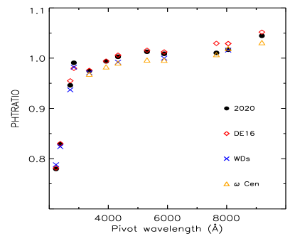
Figure 16: Comparison of old (DE16, magenta diamond) and new (2020, filled black circle) synthetic detector sensitivity ratios, PHTRATIO, with observed values computed from WD (blue cross) and $\omega$ Cen (orange triangle) observations. See text for more details.

Table 11: PHTRATIO values (PHTFLAM2/PHTFLAM1) for the WFC3-UVIS 42 full-frame filters derived from synthetic photometry by using the new (syn_2020) and the old (syn_DE16) calibration Pysynphot files, and by using observations of standard WDs and $\omega$ Cen.

Filter	Pivot	PHTRATIOsyn_2020	PHTRATIOsyn_DE16	PHTRATIOWDs	PHTRATIOωCen
F200LP	4971.86	0.998	1.0023	…	…
F218W	2228.04	0.779	0.7815	0.788	…
F225W	2372.05	0.829	0.8300	0.824	…
F275W	2709.69	0.946	0.9549	0.937	…
F280N	2832.86	0.991	0.9797	0.982	…
F300X	2820.47	0.932	0.9350	…	…
F336W	3354.49	0.975	0.9756	0.971	0.968
F343N	3435.15	0.967	0.9690	…	…
F350LP	5873.87	1.035	1.0316	…	…
F373N	3730.17	0.975	0.9663	…	…
F390M	3897.24	0.985	0.9870	…	…
F390W	3923.69	0.994	0.9942	…	0.983
F395N	3955.19	0.998	1.0031	…	…
F410M	4108.99	1.001	1.0022	…	…
F438W	4326.23	1.003	1.0059	0.992	0.990
F467M	4682.58	0.995	0.9979	…	…
F469N	4688.10	0.996	1.0082	…	…
F475W	4773.10	1.007	1.0126	…	…
F475X	4940.72	1.005	1.0121	…	…
F487N	4871.38	0.987	1.0028	…	…
F502N	5009.64	1.004	1.0187	…	…
F547M	5447.50	0.996	1.0158	…	…
F555W	5308.43	1.013	1.0013	…	…
F600LP	7468.12	1.027	1.0335	…	…
F606W	5889.17	1.009	1.0124	1.000	0.996
F621M	6218.85	1.005	1.0140	…	…
F625W	6242.56	1.000	1.0169	…	…
F631N	6304.29	0.995	1.0049	…	…
F645N	6453.59	1.005	1.0111	…	…
F656N	6561.37	0.969	1.0008	…	…
F657N	6566.63	1.000	1.0049	…	…
F658N	6584.02	0.991	1.0069	…	…
F665N	6655.88	1.012	1.0135	…	…
F673N	6765.94	1.023	1.0202	…	…
F680N	6877.60	1.019	1.0074	…	…
F689M	6876.75	1.009	1.0139	…	…
F763M	7614.37	1.020	1.0340	…	…
F775W	7651.36	1.010	1.0294	…	1.007
F814W	8039.06	1.017	1.0290	1.016	1.019
F845M	8439.06	1.009	1.0171	…	…
F850LP	9176.13	1.044	1.0518	…	1.031
F953N	9530.58	1.039	1.0231	…	…

Due to the new WFC3-UVIS inverse sensitivities being time-dependent, PHTRATIO now varies with the epoch of observation. We calculated PHTRATIO by using the PHTFLAM1 and PHTFLAM2 values at the reference epoch, June 26 2009, and results are listed in Table 11, with a comparison to DE16 PHTRATIO values. We also compared the new values with PHTRATIO calculated by using the photometry of standard star WDs dithered on the image and observed between 2010 and 2014 (Mack et al., 2015), and by using photometry from dithered images of $\omega$ Cen observed between 2009 and 2011 (Mack et al., 2013; Mack, 2016). Note that these PHTRATIO values were calculated for a 10 pixel aperture radius and no time-dependent sensitivity correction was applied; however, the observations were mostly done at the beginning of WFC3 lifetime (2009 – 2014) so the total sensitivity losses were $\approx$ 1% at most, depending on the filter. The observed PHTRATIO values derived from WD (blue crosses) and $\omega$ Cen (yellow triangles) photometry are shown in Fig. 16, where the new (2020, black filled circles) and old (DE16, magenta diamonds) synthetic PHTRATIO values are also plotted for the same filters as a function of the pivot wavelength. Table 11 and Fig. 16 show that the new PHTRATIO values agree very well with those obtained from both WD and $\omega$ Cen observations, and show improvements in several filters from the old PHTRATIO values which did not include any time-dependent sensitivity correction. The new PHTRATIO values differ slightly from those calculated using either stepped WD or dithered $\omega$ Cen observations, with an average difference of $\approx$ 0.6% and a dispersion of $\approx$ 0.7% for ten wide-band filters and one narrow-band filter (see Table 11). These differences are most likely due to the new PHTRATIO values being derived from standard star photometry in the corner sub-arrays where the flat field is less accurate. Moreover, flat field differences between opposite corners of the WFC3-UVIS detectors can be as large as $\approx$ 3% (see Table 3 in Mack 2016).

7 Comparison to the old inverse sensitivity values

We compared the new WFC3-UVIS inverse sensitivities (converted in units of magnitudes as zero points, ZPs, in the ST photometric system) with those from the 2017 calibration. The latter ZPs were calculated by using the previous CALSPEC SEDs and six years of data available for the standard stars (2009 – 2015): these measurements were simply averaged without normalizing for the sensitivity changes with time. This resulted in different reference epochs per filter, due to the different observing cadence for each detector. Additionally, the 2017 calibration did not account for differences in the observed count rates due to flat field errors. In CA21, and as reported in this work, WFC3-UVIS inverse sensitivities were derived by using new CALSPEC SEDs for the standard stars and ten years of available data (2009 – 2019). The photometric measurements of the standard stars were then normalized to a single reference epoch and weighted for photometric errors and number of measurements.

Figure 17: Comparison between the new (2020) and old (2017) ZPs for WFC3 UVIS1 (Amp A) in the ST photometric system for the wide- and medium-band filters over the entire WFC3 UVIS wavelength range. Error bars are also shown.

Figure 18: Same as Fig. 17 but for WFC3 UVIS2 (Amp C) detector.

Fig. 17 shows the comparison between new (2020) and old (2017) ZPs as a function of pivot wavelength for the wide- and medium-band UVIS1 filters. The ZPs differ on average by $\approx$ 1.5%, with the new ZPs being brighter compared to the old ones. This is mostly due to the reference flux of Vega being $\approx$ 1% brighter, and to the standard star photometry being corrected for losses in sensitivity. A similar comparison holds for the UVIS2 filters as shown in Fig. 18, where the ZPs differ on average by $\approx$ 0.9%. It is worth noting that the difference between old and new ZPs for the UVIS2 detector shows a trend between 4,000 $<\lambda<$ 8,000 Å  that is not clearly seen for UVIS1 values. This difference between the two detectors may be due to how the five standard star measurements were collected between 2009 and 2019: for most filters, Amp A (UVIS1) has more observations at the beginning, 2009-2010, and throughout WFC3 lifetime compared to Amp C (UVIS2), which has less and more sparse measurements. Since the old ZPs were calculated by simply averaging the photometry of the standard stars over the 2009 – 2015 time interval, without applying any time correction, the ZP values for UVIS2 resulted to be centered on later epochs compared to values for UVIS1.

We performed a similar comparison for WFC3-IR inverse sensitivities; the new ZPs were based on updated CALSPEC SEDs and eleven years of data available for five standard stars (2009 – 2020), compared to the previous ZPs from Kalirai et al. (2011), based on only 1.5 years of photometry for four standard stars. Furthermore, the new ZPs were calculated by using updated pixel-to-pixel flat fields to correct for spatial sensitivity residuals up to 0.5% in the center of the detector and up to 2% at the edges (Mack et al., 2021) . Also, a new set of delta flat fields was used to correct for low-sensitivity artifacts known as blobs in six filters, namely $F098M$, $F105W$, $F110W$, $F125W$, $F140W$, and $F160W$ (Olszewski & Mack, 2021). Fig. 19 shows the comparison between new (2020) and old (2012) ZPs as a function of pivot wavelength for the wide- and medium-band WFC3-IR filters. The ZPs differ on average by $\lesssim$ 1.0%, with the new ZPs being brighter compared to the old ones as expected. The comparison also shows that the difference is larger for redder filters and it is due to the new CALSPEC models differing more at longer wavelengths compared with the old ones.

Figure 19: Comparison between the new (2020) and old (2012) ZPs for WFC3-IR in the ST photometric system for the wide- and medium-band filters over the entire wavelength range. Error bars are also shown.

8 Testing the new time-dependent WFC3-UVIS inverse sensitivities

8.1 $\omega$ Cen photometry

In order to verify the precision of the new WFC3-UVIS time-dependent photometric calibration we used data collected with the $F606W$ filter for the Galactic globular cluster $\omega$ Cen over a $\approx$ 10-year time interval. Aperture photometry with a 5-pixel radius was performed on 162 _flc images and the average instrumental (cyan filled triangles) and calibrated (black filled circles) magnitude difference for all stars measured in all images versus a reference image collected in 2009 is shown as a function of observing epoch in Fig. 20. Only photometry for stars 250 pixel away from the readout amplifiers (in this case Amp C and D) is shown to mitigate the possible effects of a non perfect CTE correction. The instrumental magnitude differences (cyan triangles) were not corrected for the time sensitivity changes of the UVIS2 detector (Amp C and D) and show an increase of $\approx$ 0.02 mag over the 10-year time interval: this flux drop is expected from the calculated sensitivity loss rate of $0.02$%/yr for UVIS2 and the $F606W$ filter (see Table 4). The calibrated magnitude differences (black circles) were corrected by using the time-dependent inverse sensitivity values provided in the image header as the PHTFLAM2 keyword: as the plot in Fig. 20 shows, $\omega$ Cen magnitude differences cluster around 0, with a dispersion of $\approx$ 0.2%, as it is expected in the absence of sensitivity changes with time of the detector. We performed the same test for $\omega$ Cen UVIS1 observations and we obtained a similar result.

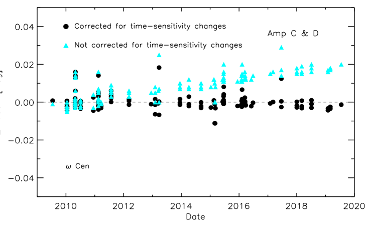
Figure 20: Instrumental (cyan filled triangles) and calibrated (black filled circles) magnitude differences between a reference UVIS2 (Amp C & D) $F606W$ image collected in 2009 for the Galactic globular cluster $\omega$ Cen and all subsequent 161 images. The instrumental magnitude differences were not corrected for time sensitivity changes, while the calibrated magnitude differences were corrected by using the time-dependent inverse sensitivity values provided in the image header as the PHTFLAM2 keyword.

8.2 Staring mode photometry

As a further validation of the time-dependent WFC3-UVIS photometric calibration, we downloaded from the Mikulski Archice for Space Telescopes (MAST) all available data in the $F814W$ filter for the standard WDs GD153 and GRW70 from 2009 until the end of 2021. These images were processed through the current calwf3 pipeline, version 3.6.2. We performed aperture photometry with a 10-pixel radius and used the header PHOTFLAM keyword to correct the observed count rates for time sensitivity changes. We then compared the observed with the synthetic count rates derived by using STsynphot and the new SEDs, in-flight and aperture corrections and filter curves for $F814W$ and UVIS1 and UVIS2, as listed in Table 7.

Fig. 21 shows the ratio of UVIS2 (Amp C) observed over synthetic count rates for GD153 (top panel) and GRW70 (bottom): the filled cyan triangles are the uncorrected ratios while the filled black circles indicate the corrected ones. The uncorrected ratios decrease with time for both stars, with a total loss of flux of $\approx$ 1.5% over almost 13 years; this is compatible with the measured sensitivity loss rate of $\approx$ 0.1%/yr for the $F814W$ filter and UVIS2. The corrected observed over synthetic count ratios cluster around 1 for both stars, with a dispersion of $\approx$ 0.33% and 0.6% for GD153 and GRW70, respectively, validating the current time-dependent inverse sensitivities values.

We performed the same test for UVIS1 observations and we obtained a similar result.

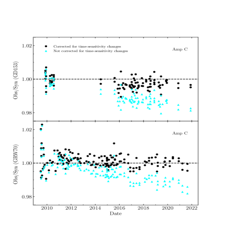
Figure 21: Staring mode $F814W$ UVIS2 (Amp C) uncorrected (cyan filled triangles) and corrected (black filled circles) observed over synthetic count rate ratios for the standard star GD153 (top panel) and GRW70 (bottom) as a function of date. The observed count rates were corrected for sensitivity changes by using the time-dependent inverse sensitivity values provided in the image header as the PHTFLAM2 keyword.

8.3 Scan mode photometry

We performed another validation test by using all available scan data for GD153 and GRW70 in the $F814W$ filter from 2017 until the end of 2021. The images were downloaded from MAST and processed with the current calwf3 pipeline and aperture photometry was performed following the recipe presented in Section 2.1.1. The count rates were corrected for sensitivity changes by using the PHOTFLAM keyword values provided in the image header.

To calculate synthetic count rates for the scan mode observations, a PSF was extrapolated from the latest $F814W$ EE curves and convolved with a scan line corresponding to the length of the spatial scan observations, thus creating a synthetic spatial scan with the same scale as the observed data. Aperture photometry was performed on the synthetic scan image, yielding a ’enrectangled’ energy correction factor. Synthetic count rates were then produced by using STsynphot with the new SEDs for GD153 and GRW70, multiplied by the synthetic ’enrectangled’ energy correction factor, the new in-flight and aperture corrections and filter curves for $F814W$ and UVIS1 and UVIS2, as listed in Table 7.

Fig. 22 shows the uncorrected (filled cyan triangles) and corrected (black filled circles) observed over synthetic count rates for UVIS2 (Amp C) for GD153 (top panel) and GRW70 (bottom): the uncorrected scan ratios are systematically lower than 1.0 by more than 1%, due to the loss of sensitivity of the detector from 2009 to 2017, and maintain a decreasing trend until the end of 2021, for a total loss of $\approx$ 1.5%. On the other hand, the corrected ratios cluster around 1 for both stars, with a dispersion of $\approx$ 0.15% (GD153) and $\approx$ 0.1% (GRW70), a factor of 2 and 6 lower, respectively, compared to the dispersion of the staring mode photometry for the same stars.

We performed the same test for UVIS1 observations and, as in the case of the staring mode observations, we obtained a similar result.

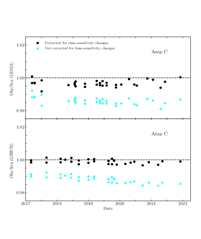
Figure 22: Scan mode $F814W$ UVIS2 (Amp C) uncorrected (cyan filled triangles) and corrected (black filled circles) observed over synthetic count rate ratios for the standard star GD153 (top panel) and GRW70 (bottom) as a function of date. The scan observation count rates were corrected for sensitivity changes by using the time-dependent inverse sensitivity values provided in the image header as the PHTFLAM2 keyword.

9 How to perform WFC3 photometric calibration

The PHOTFLAM inverse sensitivity keyword provided in the WFC3 image header can be used to convert the photometric measurements into fluxes in units of erg cm^-2 s^-1 Å^-1. For images retrieved from MAST after October 15, 2020, or re-processed after this date with the current pipeline, calwf3 version 3.6.2, the PHOTFLAM inverse sensitivity keyword includes the time-dependent correction; this can than be used to scale all the photometric measurements collected at different epochs to the reference epoch of June 26, 2009.

Magnitudes in different photometric systems can also be obtained: WFC3 provides ZPs in three systems, namely AB, ST and Vega for the reference epoch.

Magnitudes in the AB photometric system are based on a constant flux (flat spectrum) per unit frequency (Oke, 1974), with the ZP set so that VEGA has AB magnitude $\approx$ 0 in the Johnson $V$-band. Fluxes in the AB system are then defined in units of erg cm^-2 s^-1 Hz^-1, and the corresponding AB magnitude at frequency $\nu$ is defined as:

$$m(AB_{\nu})=-2.5\log(F_{\nu})-48.60$$ (6)

where the zero point is set such as AB mag = 0 is for $F_{\nu}$= 3.96$\times$10^-20 erg cm^-2 s^-1 Hz^-1.

The Space Telescope (ST) photometric system is defined in the wavelength domain and magnitudes in this systems are:

$$m(ST_{\lambda})=-2.5log(F_{\lambda})-21.10$$ (7)

where ST mag = 0 is $F_{\lambda}$ = 3.96$\times$10^-9 erg cm^-2 s^-1 Å^-1.

A characteristic wavelength, pivot wavelength, can be defined to convert flux densities from the frequency to the wavelength domain as:

$$\lambda_{p}=\sqrt{\frac{cF_{\nu}}{F_{\lambda}}}=\sqrt{\frac{\int R\lambda d\lambda}{\int R\frac{d\lambda}{\lambda}}}$$ (8)

where $R$ is the (telescope + instrument + filter) response function and $F_{\nu}$ and $F_{\lambda}$ are the fluxes in the frequency and wavelength domains. We can then transform AB to ST magnitudes using the relation:

$$m(ST_{\lambda})=m(AB_{\nu})+5log(\lambda_{p})-18.70$$ (9)

In the Vega photometric systems, magnitudes are calculated using the Vega flux as a reference:

$$m(Vega)=-2.5log(F/F_{Vega})$$ (10)

In order to convert count rates measured on WFC3 images into magnitudes, users can use the inverse sensitivity provided as the header keyword PHOTFLAM. According to the chosen photometric system, the following equations can be used to obtain the ZP at the epoch of the observation:

• ST photometric system:

  $$ZP_{STMag}=-21.1-2.5log(PHOTFLAM)$$ (11)

• AB photometric system:

  $$ZP_{ABMag}=-21.1-2.5log(PHOTFLAM)-5log(PHOTPLAM)+18.70)$$ (12)

  where PHOTPLAM is the pivot wavelength keyword, also available in the image header.

• Vega photometric system: the calculation of the ZP follows two steps. First, the user needs to calculate the flux of Vega as observed by the telescope, detector and filter, $FLAM_{Vega}$; to do this the new Vega SED should be used, alpha_lyr_stis_010.fits, available from the CALSPEC database or from the CRDS database . Subsequently, the ZP can be calculated as:

  $$ZP_{Vega}=-2.5log(PHOTFLAM/FLAM_{Vega})$$ (13)

The WFC3 team provides a Jupyter notebook that shows how to calculate the ZPs in the different photometric systems by using synphot, specifically STSynphot. Another notebook is also provided and shows how to use the new time-dependent solutions to work with WFC3-UVIS data obtained at different epochs. These notebooks are available from the WFC3 photometric calibration web page and https://www.overleaf.com/project/619d593114f0b03d31bde4b4from the STScI WFC3 Software Library on Github.

Users should note that the final photometry for both detectors will be in the UVIS1 system since WFC3 processing pipeline, calwf3, flux scales the UVIS2 detector to UVIS1 by multiplying UVIS2 by the ratio of the inverse sensitivities, PHTRATIO in the image header keyword. Therefore, users need to apply only one inverse sensitivity value, the header keyword PHOTFLAM (same as the PHTFLAM1 keyword) to calibrate their photometry.

However, UVIS1 and UVIS2 have significantly different quantum efficiencies in the UV regime ($\lambda\lesssim$ 4,000 Å), and the modified PHTRATIO introduced by DE17 to match the the count rate ratio of UVIS1 and UVIS2 for hot stars ($T_{eff}\geq$ 30,000 $K$) in the $F218W$, $F225W$, $F275W$ and $F200LP$ filters, does not work for cooler stars. Photometry for cooler stars measured on the UVIS2 detector in the UV filters thus needs to be corrected by applying a magnitude offset according to their UVIS2 color, if available, or temperature or spectral type.

Offsets for magnitudes measured on the UVIS2 detector relative to UVIS1 were calculated in the $F218W$, $F225W$, and $F275W$ filters by using synthetic photometry and observations of the globular cluster $\omega$ Cen. These are presented and available in CA18. Before applying the offset ($\Delta Mag$) to magnitudes measured on the UVIS2 detector, the photometry must be calibrated by using the provided inverse sensitivities:

$$m(ST)=-21.1-2.5log(PHOTFLAM)-\Delta Mag$$ (14)

The final photometry for both detectors will be in the UVIS1 system. If the observed sources lie in the same detector, the color term is negligible ($<$ 1%), and no magnitude offset needs to be applied.

For users who require sub-percent photometric calibration accuracy, or if observations are done by using a UVIS2 sub-array only, we recommend treating each detector separately when observing with the UV filters $F218W$, $F225W$, and $F275W$. UVIS1 magnitudes will be calibrated as usual, by applying PHOTFLAM, while the UVIS2 magnitudes will be calibrated by using PHTFLAM2. In this case, the MAST downloaded raw images (_raw.fits) will have to be re-processed manually through the calwf3 pipeline omitting the flux correction, i.e. by setting FLUXCORR = OMIT in the image header.

9.1 An example with observed data

We present here an example of how to perform the photometric calibration of WFC3 data collected at different epochs and in different filters. Observations of the LMC globular cluster NGC 1978 were collected in 2011 in the $F555W$ filter (PID: 12257), in 2016 in $F438W$ (PID: 14069), and in 2019 in $F275W$ and $F814W$ (PID: 15630). We downloaded the _flc images processed through calwf3_v3.5.2 from MAST. PSF photometry was performed with the software ePSF (Anderson & King, 2006) and corrected to a 10 pixel aperture radius; the new WFC3-UVIS EE corrections were then applied to bring the magnitudes from 10 pixels to infinity. Magnitudes were also corrected for exposure time and the new ZP for each filter and appropriate epoch of observation, as found in the PHOTFLAM image header keyword, was used to derive the final calibrated magnitudes in the Vega system. Summarizing, we obtained calibrated magnitudes, $M$, for stars in NGC 1978, from the instrumental magnitudes, $m$, as:

$$M=m+AP_{10}+EE_{inf}+2.5log(EXPTIME)+ZP_{Vega}$$ (15)

where $AP_{10}$ is the correction to bring PSF magnitudes to a 10 pixel aperture radius, $EE_{inf}$ in the EE correction from 10 pixel to infinity and $ZP_{Vega}$ was calculated as explained above.

Fig. 23 shows the calibrated $F814W,\ F275W-F814W$ (left panel), $F814W,\ F438W-F814W$ (middle) and $F814W,\ F555W-F814W$ (right) color-magnitude-diagrams (CMDs) of NGC 1978. A set of scaled-solar BaSTI isochrones for a metallicity of $Z=$ 0.0008 and different ages, namely 2, 2.5 and 3 Gyr, are over-plotted: these models were transformed to the observational plane by using the new WFC3-UVIS filter throughputs, a distance modulus range of 18.45 $\leq\mu_{0}\leq$ 18.50 mag and reddening of 0.01 $\leq E(B-V)\leq$ 0.06 mag. The figure shows that theory and observations taken over 8 years of WFC3 lifetime are in very good agreement for all filters from the UV to the optical regime: the isochrones nicely reproduce all the features of the CMD, i.e. the main-sequence, the sub-giant and red-giant branch and the horizontal branch. The comparison between models and observations provides an age range of 2-3 Gyr for NGC 1978, in agreement with previous studies based on Advanced Camera for Surveys (ACS) photometry (Martocchia et al., 2018).

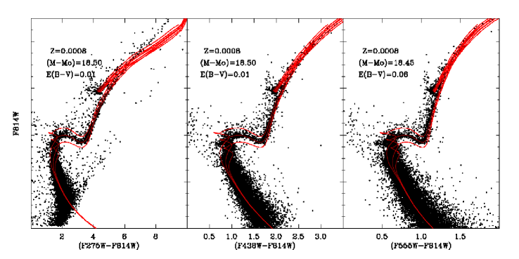
Figure 23: $F814W,\ F275W-F814W$ (left panel), $F814W,\ F438W-F814W$ (middle) and $F814W,\ F555W-F814W$ (right) CMD of the LMC globular cluster NGC 1978. A set of BaSTI isochrones with different ages and same metallicity is over-plotted. The assumed distance modulus and reddening are labeled in each panel.

10 Conclusions

In this manuscript we described how new inverse sensitivities were derived for the WFC3-UVIS and the WFC3-IR detectors. Time-dependent inverse sensitivities were derived for UVIS1 and UVIS2, for the 42 full-frame filters. They provide a photometric internal precision $\lesssim$ 0.5% for wide-, medium-, and narrow-band filters, with a significant improvement compared to the old values, where the precision was $\lesssim$ 1% for wide-, $\lesssim$ 2% for medium-, and $\lesssim$ 5 - 10% for narrow-band filters. The accuracy of the flux calibration is $\approx$ 2-3% for wide- and medium-band filter, and $\approx$ 5% for narrow-band filters.

In addition to the $\approx$ 1% error in the absolute flux calibration of the HST standards (BO20), the photometric calibration is also limited by errors in the flat field. These are typically $<$ 1% in the upper left corner of Amp A (UVIS1) but can be as large as 2% for a few filters (Mack et al., 2015; Mack, 2016). In this corner of the detector, the PSF focus is highly variable due to telescope breathing effects (Sabbi & Bellini, 2013), and this affects the accuracy of the aperture correction applied to the crowded stellar field ($\omega$ Cen) photometry used to derive the in-flight ($L$-flat) correction (Mack et al., 2013). Amp A also contains the flare, a wedge-shaped internal reflection in the ground flats at a level of 1-2%, which is strongest in the upper left corner of the UVIS1 detector (McCullough, 2011; Mack et al., 2013). These uncertainties may also impact the UVIS2 to UVIS1 inverse sensitivity ratio, i.e. PHTRATIO, since it is based on the photometry of standard stars observed in the small 512$\times$512 corner sub-arrays, where the flat field is less accurate. In the future, the WFC3 team plans to improve the flat fields by using more stellar cluster data and improved reduction techniques.

Major changes of the new WFC3-UVIS inverse sensitivities compared to the latest values delivered in 2017 can be summarized as follows:

1) The new inverse sensitivities are based on new SEDs for the standard stars and a new reference flux for Vega (see BO20);
2) EE fractions for a few filters were updated by using the time-sensitivity corrections and a new method for drizzling the standard star images. These were used in the computation of the new inverse sensitivities;
3) Four extra years (2015 – 2019) of standard star photometry were used;
4) Time-dependent corrections were calculated and standard star photometry was corrected for the sensitivity changes before deriving the inverse sensitivities. Also, the standard star observed count rates were weighted according to their photometric errors and number of collected measurements.

We also provided new inverse sensitivities for the WFC3-UVIS 20 quad filters by using the updated SEDs for the standard stars and the reference Vega flux. These values do not have a time-sensitivity correction, since not enough observations were available to calculate a sensitivity change rate. The accuracy of the calibration for these filters is $\approx$ 10-15%.

New inverse sensitivities for the 15 WFC3-IR filters were also derived by using the new SEDs, the updated reference Vega flux and 10 years of photometric data for the standard stars. These differ by $\approx$ 1.5% compared to the latest values delivered in 2011 and provide a photometric internal precision of $\approx$ 1% for all filters. The accuracy of the flux calibration is $\approx$ 2-3%.

The new time-dependent WFC3-UVIS photometric calibration was validated by using $F814W$ observations of two CALSPEC standard WDs, namely GD153 and GRW70, collected in staring and scan mode during a 12- and 3-year time frame, respectively. After applying the new time-dependent inverse sensitivities, observed over synthetic count rate ratios are, withing uncertainties, in very good agreement over the entire time intervals.

We also used observations of the globular cluster $\omega$ Cen to validate the WFC3-UVIS time-dependent calibration. Aperture photometry was performed on 162 $F606W$ exposures collected in the 2009 - 2020 time frame and the single epoch inverse sensitivities were used to correct the photometry. The magnitude differences with respect to the first reference image all cluster around zero after the correction, with a dispersion of $\approx$ 0.2%.

We also showed examples on how to derive ZPs in the AB, ST and Vega photomerric systems and how to apply the time-dependent WFC3-UVIS calibration to real observations of the cluster NGC 1978.

The new in-flight and aperture correction files for WFC3-UVIS, and the new filter curves for both WFC3 detectors were delivered to the Calibration Reference Data System (CRDS), and can be downloaded from the CRDS web page, from the STScI archive or from the synphot web page and used in synphot simulations. The models of the standard stars used in this analysis and needed for the simulations are available from the CALSPEC data repository or the aforementioned web pages (see Table 7 for a list of the file names).

New IMPHTTABs for WFC3-UVIS and WFC3-IR were also delivered, 51c1638pi_imp.fits and 4af1533ai_imp.fits, respectively. All WFC3 data were re-processed through the new version of the pipeline, calwf3_v3.5.2 as October 15, 2020, and new photometry keyword values (PHOTFLAM, and PHTFLAM1, PHTFLAM2, PHTRATIO for WFC3-UVIS) were populated in the image headers. Therefore, we recommend users to retrieve again data collected before October 2020 so that their headers will be populated with the latest inverse sensitivity values by the WFC3 processing pipeline.

The WFC3 photometric calibration web page provides the new inverse sensitivity values, calculated at the reference epoch, i.e. MJD = 55008 (June 26, 2009), for WFC3-UVIS. Values of the inverse sensitivities for UVIS1 and UVIS2 at each observing epoch can be found in the image header. However, at the same web page and on the STScI WFC3 Software Library on Github, tutorials (Jupyter notebooks) are provided for running synphot with the new filter curves in order to derive the inverse sensitivity and ZP values for any detector, observing epoch, filter or aperture. Another notebook describing how to use the new time-dependent solutions to work with WFC3-UVIS data obtained at different observation dates is also available at the same location.

In the future, the WFC3 team plans to improve the EE corrections for more filters, in particular at wavelengths longer than $\lambda\geq$ 8,000Å  and for narrow-band and long-pass filters, by using the new method illustrated in this manuscript. Also, new flat fields for the quad filters will be calculated to replace the current set of ground flats, and the inverse sensitivities recomputed. Stare and scan mode observations for different clusters are being collected with WFC3-IR to better characterize the time-sensitivity changes of this detector, if any, and new inverse sensitivities for the WFC3-IR filters will be calculated if needed.

References

- Anderson & Baggett (2014) Anderson, J. & Baggett, S. 2014, Sink Pixels and CTE in the WFC3/UVIS Detector, Space Telescope WFC Instrument Science Report
- Anderson et al. (2021) Anderson, J., Baggett, S., & Kuhn, B. 2021, Updating the WFC3/UVIS CTE model and Mitigation Strategies, Space Telescope WFC Instrument Science Report
- Anderson & King (2006) Anderson, J. & King, I. R. 2006, PSFs, Photometry, and Astronomy for the ACS/WFC, Instrument Science Report ACS 2006-01
- Bajaj (2019) Bajaj, V. 2019, WFC3/IR Photometric Repeatability, Space Telescope WFC Instrument Science Report
- Bajaj et al. (2020) Bajaj, V., Calamida, A., & Mack, J. 2020, Updated WFC3/IR Photometric Calibration, Space Telescope WFC Instrument Science Report
- Bohlin et al. (2019) Bohlin, R. C., Deustua, S. E., & de Rosa, G. 2019, AJ, 158, 211
- Bohlin et al. (2014) Bohlin, R. C., Gordon, K. D., & Tremblay, P.-E. 2014, PASP, 126, 711
- Bohlin et al. (2020) Bohlin, R. C., Hubeny, I., & Rauch, T. 2020, AJ, 160, 21
- Bradley et al. (2017) Bradley, L., Sipocz, B., Robitaille, T., et al. 2017, astropy/photutils: v0.4
- Brown (2008) Brown, T. M. 2008, WFC3 TV3 Testing: UVIS Filtered Throughput, Space Telescope WFC Instrument Science Report
- Calamida et al. (2018) Calamida, A., Mack, J., Deustua, S., & Sabbi, E. 2018, WFC3 color term transformations for UV filters, Space Telescope WFC Instrument Science Report
- Calamida et al. (2021) Calamida, A., Mack, J., Medina, J., et al. 2021, New time-dependent WFC3 UVIS inverse sensitivities, Space Telescope WFC Instrument Science Report
- Carlberg & Monroe (2017) Carlberg, J. K. & Monroe, T. 2017, Updated Time Dependent Sensitivity Corrections for STIS Spectral Modes, Space Telescope STIS Instrument Science Report
- Dahlen (2013) Dahlen, T. 2013, WFC3/IR Spatial Sensitivity Test, Space Telescope WFC Instrument Science Report
- Deustua et al. (2017a) Deustua, S. E., Bohlin, R. C., Mack, J., et al. 2017a, WFC3 Chip Dependent Photometry with the UV filters, Space Telescope WFC Instrument Science Report
- Deustua et al. (2017b) Deustua, S. E., Mack, J., Bajaj, V., & Khandrika, H. 2017b, WFC3/UVIS Updated 2017 Chip-Dependent Inverse Sensitivity Values, Space Telescope WFC Instrument Science Report
- Deustua et al. (2016) Deustua, S. E., Mack, J., Bowers, A. S., et al. 2016, UVIS 2.0 Chip-dependent Inverse Sensitivity Values, Space Telescope WFC Instrument Science Report
- Gennaro et al. (2018) Gennaro, M., Bajaj, V., & Long, K. 2018, A characterization of persistence at short times in the WFC3/IR detector, Tech. rep.
- Gosmeyer & Baggett (2016) Gosmeyer, C. M. & Baggett, S. 2016, WFC3/UVIS External CTE Monitor: Single-Chip CTE Measurements, Space Telescope WFC Instrument Science Report
- Hartig (2009a) Hartig, G. F. 2009a, WFC3 SMOV Programs 11436/8: UVIS On-orbit PSF Evaluation, Space Telescope WFC Instrument Science Report
- Hartig (2009b) Hartig, G. F. 2009b, WFC3 SMOV Programs 11437/9: IR On-orbit PSF Evaluation, Space Telescope WFC Instrument Science Report
- Hilbert (2009) Hilbert, B. 2009, WFC3 SMOV Program 11427: UVIS Channel Shutter Shading, Tech. rep.
- Hubeny (2017) Hubeny, I. 2017, MNRAS, 469, 841
- Kalirai et al. (2010) Kalirai, J. S., Cox, C., Dressel, L., et al. 2010, WFC3 Pixel Area Maps, Space Telescope WFC Instrument Science Report
- Kalirai et al. (2011) Kalirai, J. S., Deustua, S., Rajan, A., & Riess, A. 2011, The Photometric Performance of WFC3/IR: Temporal Stability Through Year 1, Space Telescope WFC Instrument Science Report
- Kalirai et al. (2009a) Kalirai, J. S., MacKenty, J., Bohlin, R., et al. 2009a, WFC3 SMOV Proposal 11451: The Photometric Performance and Calibration of WFC3/IR, Space Telescope WFC Instrument Science Report
- Kalirai et al. (2009b) Kalirai, J. S., Saul Davis, D., Richer, H. B., et al. 2009b, ApJ, 705, 408
- Khandrika et al. (2018) Khandrika, H., Deustua, S., & Mack, J. 2018, WFC3/UVIS - Temporal and Spatial Variations in Photometry, Space Telescope WFC Instrument Science Report
- Koornneef et al. (1986) Koornneef, J., Bohlin, R., Buser, R., Horne, K., & Turnshek, D. 1986, Highlights of Astronomy, 7, 833
- Kozhurina-Platais & Baggett (2020) Kozhurina-Platais, V. & Baggett, S. 2020, WFC3 IR sensitivity over time, Space Telescope WFC Instrument Science Report
- Long et al. (2013) Long, K. S., Baggett, S. M., & MacKenty, J. W. 2013, Characterizing Persistence in the WFC3 IR Channel: Finite Trapping Times, Space Telescope WFC Instrument Science Report
- Long et al. (2011) Long, K. S., Wheeler, T., & Bushouse, H. 2011, IR Detector Timing and Persistence, Tech. rep.
- Mack (2016) Mack, J. 2016, UVIS 2.0: Ultraviolet Flats, Space Telescope WFC Instrument Science Report
- Mack et al. (2021) Mack, J., Olszewksi, H., & Pirzkal, N. 2021, WFC3/IR Filter-Dependent Sky Flats, Space Telescope WFC Instrument Science Report
- Mack et al. (2015) Mack, J., Rajan, A., & Bowers, A. 2015, Spatial Accuracy of the UVIS Flat Fields, Space Telescope WFC Instrument Science Report
- Mack et al. (2013) Mack, J., Sabbi, E., & Dahlen, T. 2013, In-flight Corrections to the WFC3 UVIS Flat Fields, Space Telescope WFC Instrument Science Report
- Martocchia et al. (2018) Martocchia, S., Niederhofer, F., Dalessandro, E., et al. 2018, MNRAS, 477, 4696
- McCullough (2011) McCullough, P. 2011, Geometric model of UVIS window ghosts in WFC3, Instrument Science Report WFC3 2011-16, 28 pages
- Oke (1974) Oke, J. B. 1974, ApJS, 27, 21
- Olszewski & Mack (2021) Olszewski, H. & Mack, J. 2021, WFC3/IR Blob Flats, Space Telescope WFC Instrument Science Report
- Rauch et al. (2013) Rauch, T., Werner, K., Bohlin, R., & Kruk, J. W. 2013, A&A, 560, A106
- Rieke et al. (2008) Rieke, G. H., Blaylock, M., Decin, L., et al. 2008, AJ, 135, 2245
- Ryan & Baggett (2015) Ryan, R. E., J. & Baggett, S. M. 2015, The Internal Flat Fields for WFC3/IR, Space Telescope WFC Instrument Science Report
- Sabbi (2009) Sabbi, E. 2009, WFC3 SMOV Program 11798: UVIS PSF Core Modulation, Tech. rep.
- Sabbi & Bellini (2013) Sabbi, E. & Bellini, A. 2013, UVIS PSF Spatial & Temporal Variations, Instrument Science Report WFC3 2013-011, 10 pages
- Sahu et al. (2014) Sahu, K., Baggett, S., & MacKenty, J. 2014, Use of the Shutter Blade Side for UVIS Short Exposures, Tech. rep.
- Sahu et al. (2015) Sahu, K., Gosmeyer, C. M., & Baggett, S. 2015, WFC3/UVIS Shutter Characterization, Tech. rep.
- Shanahan et al. (2017a) Shanahan, C. E., Gosmeyer, C. M., & Baggett, S. 2017a, 2017 Update on the WFC3/UVIS Stability and Contamination Monitor, Space Telescope WFC Instrument Science Report
- Shanahan et al. (2017b) Shanahan, C. E., McCullough, P., & Baggett, S. 2017b, Photometric Repeatability of Scanned Imagery: UVIS, Space Telescope WFC Instrument Science Report
- Som et al. (2021) Som, D., Bajaj, V., Mack, J., & Calamida, A. 2021, Photometric Repeatability and Sensitivity Evolution of WFC3/IR, Space Telescope WFC Instrument Science Report
- Stetson (1987) Stetson, P. B. 1987, PASP, 99, 191
- STScI Development Team (2018) STScI Development Team. 2018, synphot: Synthetic photometry using Astropy
- The Astropy Collaboration et al. (2018) The Astropy Collaboration, Price-Whelan, A. M., Sipőcz, B. M., et al. 2018, ArXiv e-prints