Learning of error statistics for the detection of quantum phases

Abstract

We present a binary classifier based on neural networks to detect gapped quantum phases. By considering the errors on top of a suitable reference state describing the gapped phase, we show that a neural network trained on the errors can capture the correlation between the errors and can be used to detect the phase boundaries of the gapped quantum phase. We demonstrate the application of the method for matrix product state calculations for different quantum phases exhibiting local symmetry-breaking order, symmetry-protected topological order, and intrinsic topological order.

I Introduction

The classification of quantum phases at zero temperature is one of the most important tasks in condensed matter physics. While phases characterized by local order parameters can be successfully described in terms of spontaneous symmetry breaking Landau (2008), the discovery of topological phases without local order presents a significant challenge in this endeavor. Here, we show that the notion of an order parameter can be also transfered to such exotic phases, by representing the classification of ground states of gapped quantum phases as a binary classification problem for a neural network.

In recent years, algorithms based on machine learning have also been found useful in the study of condensed matter physics where different supervised and unsupervised algorithms have been employed to analyze both classical Carrasquilla and Melko (2017); Beach et al. (2018) and quantum phase transitions Dong et al. (2019); Zhang et al. (2017); Zhang and Kim (2017); Broecker et al. (2017); Huang et al. (2021), to compute the ground state wavefunctions Carleo and Troyer (2017); Deng et al. (2017a) and their properties Deng et al. (2017b). While efforts are in progress to apply classical machine learning algorithms to gain insights into quantum systems, there has also been interest in the emerging field of quantum machine learning Biamonte et al. (2017) where quantum variants of the classical machine learning concepts are being proposed with applications in condensed matter physics Cong et al. (2019) and quantum information Beer et al. (2020, 2021).

In this article, we introduce an approach to quantify the amount of local or nonlocal order in a quantum state, based on a machine learning method. Our approach is motivated by the characterization of errors on top of an ordered reference state in the recently introduced operational definition for topologically ordered quantum phases Jamadagni and Weimer (2020). By employing conventional neural networks, we propose a classification scheme resulting in an binary classifier capable of detecting gapped quantum phases. In Sec. II, we briefly review the operational definition and present possible generalizations. Furthermore, we outline the machine learning based method capable of detecting different gapped phases. To demonstrate the above introduced method, we apply this to detect quantum phases with local order in Sec. III, symmetry-protected topological (SPT) order in Sec. IV.1, intrinsic topological order in Sec. IV.2 and their associated phase transitions. Furthermore, in Sec. V, we discuss the ability of a neural network trained on the errors of a one quantum phase to detect another quantum phase with similar error correlations. Finally, in Sec. VI, we summarize the results while also providing few directions that can be further explored using our machine learning based method.

II Learning from the operational definition of topological order

In the following, we introduce our method to detect gapped quantum phases, which is inspired by the operational definition for topological order Jamadagni and Weimer (2020). We therefore briefly review this approach and extensions to phases exhibiting local order Jamadagni and Weimer (2021). Essentially, this operational definition interprets topological order as the intrinsic ability of a system to perform topological error correction and classifies topological phases in terms of reference states without any errors. An important step is the identification of errors on top of the reference state. Following the identification of the errors, it further requires defining an error correction circuit which annihilates all errors, thereby projecting back to the reference state. States are classified as topologically ordered if the quantum state under consideration can be corrected to the reference state by a circuit whose depth remains finite in the thermodynamic limit, i.e., the time required to complete the error correction does not diverge. To summarize, the operational definition has two parts: (i) identification of an appropriate excitation basis for the errors with respect to a reference state and (ii) an appropriate error correction circuit leading to the computation of the circuit depth. In the present article, we provide a drastic simplification of the second step in the operational definition, by removing the requirement to construct an error correction circuits and replacing it with a machine learning approach.

The operational definition can be generalized towards phases exhibiting symmetry-protected topological order and phases undergoing spontaneous symmetry breaking exhibiting local order parameters, by imposing symmetry constraints on the error correction circuits Jamadagni and Weimer (2021). In the following, we will also discuss how these generalizations can be implemented within our machine learning approach.

Figure 1: Scheme for machine learning of gapped quantum phases. (a) As the first step, the ground state wave function is sampled in the error basis, yielding a classical set of measurement results for each sample. (b) The error sets sampled deep inside the ordered (trivial) phase are labeled as 1 (0) and are passed as inputs to train a Deep Neural Network (DNN). To extract the critical point, we sample the wavefunction at intermediate strengths $h$, i.e., outside the regime used for the training of the DNN. The prediction probablity for the ordered phase, $P_{1}$, can serve as a binary classifier for the phase transition.

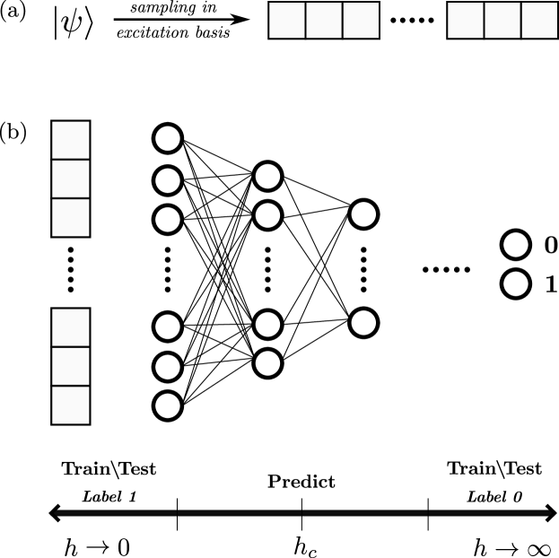
The depth of the error correction circuit fundamentally captures the deconfinement of the errors, which signals the breakdown of the ordered phase. This deconfinement is contained in the correlations between the errors and provides a natural way to employ machine learning for the classification of quantum phases. Neural network-based algorithms belonging to the class of supervised machine learning algorithms have been effective in capturing correlations in data and therefore are suitable candidates for the task of learning the correlations between the errors. The key advantage of employing such neural network-based classifiers is that they are not only efficient at learning the correlations but also that the trained neural network is capable of classifying errors sampled on a wavefunction which is different from the one used for training the neural network. In other words, given any state and the errors obtained by sampling in the excitation basis defined with respect to a reference state, the trained neural network is capable of predicting whether the given state belongs to the same phase as the reference state.

Learning the properties of the error correlations requires the generation of suitable training data. For this, we weakly perturb the reference state as well as a disordered paramagnetic state, for which we know which phase the resulting states are in. Using a Monte-Carlo sampling Jamadagni and Weimer (2021), we obtain simulated measurement data representing snapshots of the errors in the perturbed ground state. This training set is then fed into a deep neural network (DNN), see. Fig. 1, which is trained using standard machine learning algorithms for classification problems. The binary output variable of the DNN is given by the classification into the ordered phase connected to the reference state (1) or the disordered paramagnet (0). The trained network is then used to predict at which strength of the perturbation the errors become deconfined, i.e., where the phase transition takes place. The prediction probability for the ordered state, $P_{1}$, can then be interpreted as a binary classifier for the phase boundary, as at criticality, the neural network becomes confused van Nieuwenburg et al. (2017) and $P_{1}\approx P_{0}\approx 0.5$.

III Detecting quantum phases with local order

Quantum phases with local order respect the Landau symmetry breaking principle and thus the phase transition can be characterized by a local order parameter. One of the paradigmatic model encoding such a phase transition is the Ising model in the presence of a transverse field. Here, we consider a spin-1/2 chain with open boundary conditions with an antiferromagnetic (AFM) nearest neighbor interaction $(J>0)$ in the presence of a transverse field, whose Hamiltonian is given by

$$H_{\text{TFI}}=J\sum\limits_{i}^{N-1}\sigma_{z}^{i}\sigma_{z}^{i+1}-h_{x}\sum\limits_{j}^{N}\sigma_{x}^{j}.$$ (1)

This model has been extensively analyzed in the literature, and it is well known that in the limit of $J\gg h_{x}$, the ground state exhibits antiferromagnetic order, while in the limit of $J\ll h_{x}$, the ground state is a paramagnet with the spins aligned in the $x$-direction. The critical point for the phase transition is located at $h_{x}/J=1$. For convenience, we set $J=1$ in the following.

III.1 Errors associated with the AFM phase

For applying the machine learning procedure, we begin by first introducing the errors associated to the AFM phase. To this extent, we consider the degenerate ground state in the antiferromagnetic limit of $h_{x}/J\rightarrow 0$ in Eq. 1 given by $|1010...10\rangle$ or by $|0101...01\rangle$, where $0$ and $1$ denote a spin pointing down and up, respectively. The errors in the state are identified by the presence of domain walls which appear when two neighbors have the same spin. As the transverse field is turned on, the perturbed ground states exhibit virtual domain wall excitations. Below the transition, the domain walls are bound, while above the transition the domain walls become free and proliferate through the entire system. Hence, the phase transition can be understood as a confinement-deconfinement transition of the domain walls and the correlations between the domain walls can be used to characterize the AFM phase.

Having introduced the notion of domain walls, i.e., errors associated with the AFM phase, we now outline the procedure to generate errors at a finite strength of the transverse field $h_{x}$. For this, we consider the Matrix Product State (MPS) representation of the perturbed ground state computed using the Density Matrix Renormalization Group (DMRG) algorithm using the ITensor libraryFishman et al. (2020). We sample the MPS computed at various strengths of the transverse field in the $\sigma_{z}$ basis, i.e., given an MPS we simulate the measurement outcomes using a Monte-Carlo technique as in Refs. Han et al., 2018; Jamadagni and Weimer, 2021. From the sampled data, we construct the errors by observing the nearest neighbor of a given site and denote the presence (absence) of domain wall with 1 (0).

III.2 Training a DNN with errors

To recognize the correlations between the errors, we turn to supervised machine learning algorithms and employ a DNN. A DNN is characterized by an input layer, output layer and multiple hidden layers with each layer consisting of multiple nodes. These nodes are further connected by edges which carry a weight. Here, we consider an all-to-all connected DNN i.e., all the nodes are interconnected. As DNNs belong to the class of supervised machine learning algorithms, a labeled dataset is required for the purposes of training i.e., optimizing the variable weighted edges to map the input data to their appropriate labels. To estimate the performance of a DNN, we randomly split the labeled dataset into training and validation datasets, with the former being used for training and the latter being used to benchmark the training.

Having introduced the key ingredients of DNNs, we now outline the procedure to train the errors of the AFM phase at a finite field strength $h_{x}$. For our training prodcuedure, we need labeled inputs to train and validate the DNN. For this, we sample the ground state of Eq. 1 at various $h_{x}$ deep inside the AFM phase, i.e., $0.25<h_{x}<0.75$, and deep in the trivial phase, i.e.,$1.5<h_{x}<2$, to construct the respective errors. We then label the errors in the AFM (trivial) phase with 1 (0) for the purpose of training the DNN. For details on the structure of the DNN, a binary classifier, and other associated training parameters, see App. A.

(a)

(b)

(c)

Figure 2: Detecting antiferromagnetic order using machine learning. (a) Classification probability $P_{1}$ for antiferromagnetic order close to the phase transition and outside of the training regime. The probability of measured errors belonging to the AFM phase is 1 below the transition and approaches zero above the critical point. The inset shows the finite size scaling analysis for the critical value, leading to $h_{c}=1.001(1)$ (b) $P_{1}$ for a DNN trained on the errors of the AFM phase of the transverse field Ising model is used to detect the antiferromagnetic order in the presence of a longitudinal field. (c) The same DNN is used to map out the AFM phase in the Extended Bosonic SSH model, captured results in (b) and (c) are shown for $N=100$ spins.

III.3 Detecting quantum criticality using a DNN

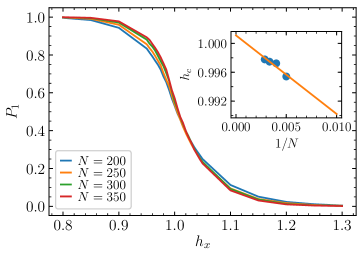
In the following, we will be interested to determine the critical point of the phase transition between the AFM and the paramagnet using our trained DNN. For this, we sample the MPS representation of the ground state wave function at different intermediate values of the field strength $h_{x}$. The resulting errors are classified by the trained DNN, resulting in a probability $P_{1}$ for the classification in the ordered phase. Likewise, $P_{0}$ represents the probability for the classification in the disordered phase. As shown in Fig. 2(a), $P_{1}$ is very close to one until one gets very close to the quantum phase transition. The location of the phase transition can be further narrowed down by a finite size scaling analysis. The inset of Fig. 2(a) shows the position of the maximum of $\partial P_{1}/\partial h_{x}$, predicting the critical point to be located at $h_{x}=1.001(1)$, which is in excellent agreement with the exact value of $h_{x}=1$. Remarkably, the accuracy of the DNN on the training and the validation dataset is close to 100% leading to negligible error bars in the finite size scaling analysis.

III.4 Detecting antiferromagnetic order under different perturbations

One of the significant features of the introduced machine learning method is that the trained DNN can now be utilized to detect antiferromagnetic order under different perturbations. To demonstrate this, we consider two cases: (a) The Ising model in the presence of both a transverse and a longitudinal field, (b) an extended bosonic Su-Schrieffer–Heeger (SSH) model. Here, we detect the phase boundaries for AFM order based on the DNN trained on the Ising model in only a transverse field. Again, we sample the perturbed ground states to construct the errors formed by domain wall excitations and pass the Monte-Carlo samples into the trained DNN for binary classification in terms of the classification probability $P_{1}$.

III.4.1 Ising model with transverse and longitudinal field

As the first case, we add an additional longitudinal field $h_{z}$ to the transverse field Ising model $H_{\text{TFI}}$ of Eq. (1), i.e.,

$$H_{\text{TLFI}}=H_{\text{TFI}}-h_{z}\sum\limits_{j}^{N}\sigma_{z}^{j}.$$ (2)

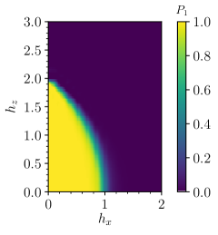
We sample the MPS representation of the ground state wave function obtained using the DMRG algorithm at different strengths of $h_{x}$ and $h_{z}$. We construct the corresponding errors from the sampled wavefunction and provide these as input to the trained DNN to obtain the classification probability $P_{1}$ for AFM ordering. The phase diagram computed within our machine learning method is shown in Fig. 2(b), which is in strong agreement with the previously established phase diagram using a local order parameter Ovchinnikov et al. (2003). The trained DNN is capable of not only detecting the second order phase transition at $h_{z}\neq 0$ and $h_{x}\neq 0$ but also detects the first order phase transition phase transition at $h_{z}\neq 0$ and $h_{x}=0$. Extracting the order of the phase transition using the machine learning remains an open task for future work.

III.4.2 Extended bosonic SSH model

The Hamiltonian of the extended bosonic SSH model Elben et al. (2020) is given by

$$\begin{split}H_{\text{BSSH}}&=\frac{v}{2}\sum\limits_{i=1}^{N/2}\big{(}\sigma^{2i-1}_{x}\sigma^{2i}_{x}+\sigma^{2i-1}_{y}\sigma^{2i}_{y}+\delta\sigma^{2i-1}_{z}\sigma^{2i}_{z}\big{)}\\ &+\frac{w}{2}\sum\limits_{i=1}^{N/2-1}\big{(}\sigma^{2i}_{x}\sigma^{2i+1}_{x}+\sigma^{2i}_{y}\sigma^{2i+1}_{y}+\delta\sigma^{2i}_{z}\sigma^{2i+1}_{z}\big{)}.\end{split}$$ (3)

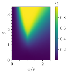
While the model is mostly interesting for its topological properties, see below, it also features an AFM phase for large values of $\delta$. As in the earlier case, we sample the MPS representation of the ground state wavefunction at various strengths of the tuple $(w/v,\delta)$. The errors associated with the AFM phase are passed as inputs to the trained DNN output $P_{1}$ as before. The antiferromagnetic order computed using the DNN in Fig. 2(c) is in strong agreement with the phase diagram established using other methods Elben et al. (2020); Jamadagni and Weimer (2021). Hence, we have demonstrated that a DNN trained with a certain perturbation of the reference state is capable of detecting the gapped phase in the presence of different perturbations.

While it is in general straightforward to work with local order parameters for phases exhibiting spontaneous symmetry breaking, another key feature of our approach is that it can be extended to gapped quantum systems with topological order, which we shall explore in the next section.

IV Detecting quantum phases with topological order

Let us now establish that the machine learning method is also capable of detecting topological phases of matter, which are beyond the conventional Landau symmetry breaking principle. Many different topological states of matter have been discovered Wen (2019) and their classification remains an important problem. In the following, we limit our discussion to models exhibiting symmetry-protected topological (SPT) order and intrinsic topological order. In the following, we briefly review the notion of topological order based on entanglement properties of the respective phases captured via the local unitaries connecting them to a product state Chen et al. (2010). In this notion, one considers the properties of a quantum circuit comprised of a sequence of quasi-local unitary operations. States having topological order are said to be long-range entangled, i.e., any circuit that takes a topologically ordered state to a product state has to have a circuit depth that diverges in the thermodynamic limit.

IV.1 Detecting symmetry-protected topological order

Importantly, not all short-range entangled states that can be connected to a product state by a finite-depth quantum circuit are topologically trivial. If one imposes symmetries on the quantum circuits, it is possible that a short-range entangled state can only be connected to a product state by symmetry-preserving circuits whose depth diverges in the thermodynamic limit. These states are said to have symmetry-protected topological (SPT) order. In the context of the recently introduced operational definition Jamadagni and Weimer (2021), a state is said to be SPT ordered if it can be corrected by a symmetry preserving finite-depth error correction circuit. In the following, we introduce the machine learning based order parameter to detect SPT phases in the variants of the SSH model.

IV.1.1 Phase transitions in the SSH model

One of the well known models exhibiting SPT order is the SSH model Su et al. (1980), whose Hamiltonian describes the hopping of a particle on a one-dimensional lattice, see Fig. 3. We consider a hardcore boson variant, which is given by the $\delta=0$ case of Eq. (3), i.e.,

$$H_{\text{SSH}}=v\sum\limits_{i=1}^{N/2}\sigma_{-}^{2i-1}\sigma_{+}^{2i}+w\sum\limits_{i=1}^{N/2-1}\sigma_{-}^{2i}\sigma_{+}^{2i+1}+\text{h.c.}.$$ (4)

Figure 3: The SSH Hamiltonian describes the hopping of particles on a 1D lattice with the choice of the unit cell as AB/BA and hopping strengths between the rails $A$ and $B$, given by $v$ and $w$, respectively.

(a)

(b)

(c)

Figure 4: Probing SPT phases in the SSH model and the extended bosonic SSH model. (a) Classification probability $P_{1}$ for the $v<w$ SPT phase as a function of the hopping strength ratio, $v/w$, for the choice of the unit cell as $AB$. The inset shows the finite size scaling analysis for the critical value, leading to $v_{c}=1.003(2)w$. (b) Using the DNN trained on the errors sampled with respect to the reference state $|\psi\rangle_{\text{AB}}$ of the SSH model, we predict the corresponding SPT phase in the extended bosonic SSH model by computing $P_{1}$ as a function of the hopping strength ratio $w/v$ and AFM interaction strength $\delta$. (c) Using the DNN trained on the errors on top of the reference state $|\psi\rangle_{\text{BA}}$, we map out the extent of the $v>w$ SPT phase. A system size of $N=100$ is used for computing the phase diagram in (b) and (c).

The SSH Hamiltonian has been extensively studied, in the case of periodic boundary conditions where the Hamiltonian is exactly solvable with gapped phases in both the limits of $v<w$ and $v>w$ with a gap closing at $v=w$ signaling a phase transition. Additionally, the limit of $v<w$ and $v>w$ have non-vanishing winding number, $\nu=1$, which is a characteristic feature of the topological phase. In the case of open boundaries, in the limit of $v\ll w$ we have edge modes at the end of the chain which characterize topological order with topological phase transition at $v=w$. Within the operational definition, one can show that the phase in the case $v>w$ is also SPT ordered, which is distinct from the SPT ordered phase characterized by edge modes Jamadagni and Weimer (2021).

Having briefly reviewed the key features of the SSH model, we turn to the machine learning method introduced earlier to train a DNN to probe SPT phases and their respective phase transitions. To train the DNN, we need to generate the errors associated with a SPT phase. For this, we briefly review the notion of errors related to the SPT phase as introduced in the Ref. Jamadagni and Weimer, 2021. For both SPT phases, the reference states are found by setting either $w=0$ or $v=0$. Then, the ground state can be found by putting singlets on the $AB$ ($BA$) unit cells, i.e.,

$$|\psi\rangle_{\text{AB/BA}}=\frac{1}{\sqrt{2}}\prod\limits_{i\in B/A}(|0\rangle_{i}|1\rangle_{i+1}-|1\rangle_{i}|0\rangle_{i+1}).$$ (5)

We can introduce an excitation basis for each unit cell, consisting of the error-free state $|\bm{-}\rangle=(|01\rangle-|10\rangle)/\sqrt{2}$ as well as density fluctuations $|\bm{0}\rangle=|00\rangle$ and $|\bm{1}\rangle=|11\rangle$, and phase fluctuations $|\bm{+}\rangle=(|01\rangle+|10\rangle)/\sqrt{2}$. In the following, we discuss the case of the unit cell choice being $AB$, leading to SPT ordered phase in the limit of $v<w$ which is characterized by the presence of edge modes.

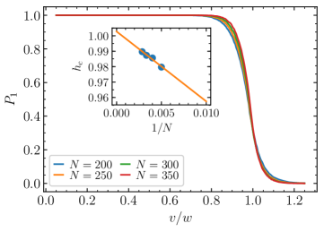
The errors in the system correspond to the density fluctuations $|\bm{0}\rangle,|\bm{1}\rangle$ and the phase fluctuation $|\bm{+}\rangle$. We construct the errors by sampling the MPS representation of the ground state wavefunction in the excitation basis at finite $v$. For the sake of training the DNN, we label the errors $\bm{0},\bm{1},\bm{+},\bm{-}$ as $\{0,1,2,-1\}$, with the outputs generated in the limit of $v<w$ ($v>w$) labeled as 1 (0). As earlier, $P_{1}$ i.e., the probability of errors being labeled as 1 captures the phase transition. By performing finite size scaling analysis, we extract the critical value for $v$, see Fig. 4, and note it to be in good agreement with the exact result $v=w$.

The discussion on choosing the other unit cell i.e., the $BA$ unit cell, leading to the detection of the $v>w$ SPT is similar. The key difference between the two scenarios is that, in the previous limit for training purposes we label the errors in the limit of $v<w$ ($v>w$) to be 1 (0) while in the current scenario we invert the above by labeling the errors in the limit of $v>w$ ($v<w$) to be 1 (0). Training and constructing the DNN, as well as extracting the critical point can be performed in exactly the same way.

IV.1.2 Detecting SPT order in the Extended Bosonic SSH model

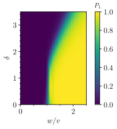
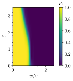
Let us now turn to the extended bosonic SSH model of Eq. 3 with nonzero antiferromagnetic interaction $\delta$. In particular, we are interested in the fate of the two SPT phases upon increasing $\delta$, using the trained DNNs from the previous section, which encodes the error correlations of the SPT phases for $\delta=0$ and $v<w$ and $v>w$, respectively. To this extent, we consider the MPS representation of the ground state of the Hamiltonian as a function of the tuple $(w/v,\delta)$. We then sample the MPS representation in the excitation basis defined with respect to the reference state to generate the errors associated with the SPT phases in the limit of $v<w$ and $v>w$ as introduced in Eq. (5). In Fig. 4(b, c), we plot $P_{1}$, the probability of sampled errors being labeled as 1, in the $v<w$ ($v>w$) regime thereby detecting the SPT phase corresponding to $v<w$ ($v>w$) of the Extended Bosonic SSH Hamiltonian. The phase diagram of the extended bosonic SSH model computed using the neural network-based method is in very good agreement with other methods Elben et al. (2020); Jamadagni and Weimer (2020).

IV.2 Intrinsic Topological order

In contrast to symmetry-protected topological order, intrinsic topological order refers to states that cannot be mapped onto product states by a finite-depth quantum circuit, even if arbitrary quasi-local unitaries are allowed. In the context of the operational definition, topological order is quantified by the error correcting abilities of a state. Formally, the operational definition quantifies a state to be topologically ordered if it can be corrected by a finite-depth error correction circuit Jamadagni and Weimer (2020). One of the paradigmatic models exhibiting intrinsic topological order is the toric code model Kitaev (2003). In the following, we briefly introduce variants of the toric code model and discuss the robustness of topological order in various perturbed toric code models using the machine learning method.

(a)

(b)

(c)

Figure 5: (a) Toric code with rough open boundaries with the vertex and face operators given by $A_{v}$ (green diamond), $B_{p}$ (blue diamond) and $B_{p^{\prime}}$ (light blue diamond). The anticommutators of $A_{v}$ ($B_{p/p^{\prime}}$) given by $\sigma_{z(x)}$ generate the vertex (face) excitations denoted by red (orange) squares. (b) Classification probability $P_{1}$ for topological order, as predicted by the trained DNN, as a function of the external perturbation strength, $h_{x}$. The inset shows the phase transition between the topologically ordered phase and the trivial paramagnet to occur at $h_{c}^{ml}=0.401(3)$. (c) Standard deviation $\sigma$ of the error correction circuit depth according to the operational definition for topological order, resulting in a critical strength of $h_{c}^{od}=0.405(8)$ (inset). Results are shown for a $L_{y}\times L_{x}$ lattice, where $L_{y(x)}$ is the number of rows (columns). We fix $L_{y}=5$ while varying $L_{x}$, with the total number of spins, $N$, given by $(2L_{y}+1)\times L_{x}+L_{y}$.

IV.2.1 Phase transitions in the toric code model

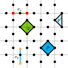
To introduce the toric code model, we consider a square lattice with open boundary conditions with spins on the edges as in Fig. 5. The Hamiltonian is given by

$$H_{\text{TC}}=-\sum\limits_{v}A_{v}-\sum\limits_{p}B_{p}-\sum\limits_{p^{\prime}}B_{p^{\prime}},$$ (6)

where $A_{v}=\prod_{i}\sigma_{x}^{i}$, $B_{p}=\prod_{j}\sigma_{z}^{j}$, for $i,j$ being the spins attached to the vertex $v$ and face $p$ respectively. The open boundaries in terms of $B_{p^{\prime}}$ operators, which realizes a three-body $\sigma_{z}$ interaction, in contrast of the four-body interaction of $B_{p}$. Such boundary conditions are generally referred to as rough boundaries, for a more detailed description on various boundary conditions associated with the toric code, we refer the reader to Ref. Beigi et al., 2011. The ground state of the toric code Hamiltonian on a planar geometry with rough boundaries is given by $\mathcal{N}\prod\limits_{v}(\mathds{1}+A_{v})|\textbf{0}\rangle$, where $|\textbf{0}\rangle=|000...0\rangle$. The excitations in the system are generated by the action of the anticommutators of $A_{v}$ ($B_{p}$) given by $\sigma_{z(x)}$ on the ground state and are identified as vertex (face) excitations.

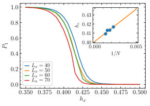
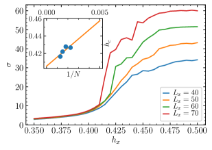
To demonstrate the machine learning based method, we consider the toric code with rough boundaries in the presence of an external magnetic field pointing in the $x$ direction, leading to the Hamiltonian, $H_{\text{PTC}}=H_{\text{TC}}-h_{x}\sum_{i}\sigma_{x}^{i}$. In the limit of $h_{x}\rightarrow 0$, the phase is topologically ordered while in the limit of $h_{x}\rightarrow\infty$ we have a paramagnetic phase. To capture the phase transition using the DNN, we compute the MPS representation of the ground state wavefunction as a function of the perturbation strength $h_{x}$, using a DMRG algorithm. We then sample the wavefunction in the $\sigma_{z}$ basis to construct the errors. Observing the fact the perturbation only anticommutes with the $B_{p}$ operator, we conclude that the system only hosts face excitations. To capture the face excitations and therefore to construct the errors, it is sufficient to compute the parity of ones in each face by measuring each spin in the $\sigma_{z}$ basis. Even (odd) parity of ones indicates the absence (presence) of excitation leading to construction of the errors. As established earlier, we label the errors in the topological (trivial) phase as 1 (0) to train the DNN. The trained DNN is now exposed to errors sampled outside of the training regime and $P_{1}$, the probability of errors being labeled as 1, capture the phase transition, with the critical strength being computed by performing finite size scaling analysis, as in Fig. 5. To validate the transition point obtained by the machine learning method, we compare it with the critical value obtained from the operational definition, see Fig. 5. We note the values for the critical perturbation strength obtained using both methods are in good agreement and therefore further validate the machine learning based method. Furthermore, we would like to point out that, for the same number of samples, $P_{1}$ obtained from machine learning exhibits significantly less noise than the standard deviation of the circuit depth $\sigma$ within the operational definition, i.e., the machine learning approach requires less computational resources for the same level of accuracy. For the details on the error correction circuit used to extract the time statistics, see App. B.

V Detecting other gapped phases with similar errors

In the previous sections, we have established that a DNN trained on the errors of a gapped quantum phase is capable of detecting the same phase even if the perturbation is changed. As introduced in Sec. II, a gapped quantum phase has a correspondence with the associated errors and their correlations. However, a DNN trained on the error correlations of a gapped phase is still capable of recognizing other gapped quantum phases with similar error correlations. For instance, consider gapped phases $A$ and $B$ whose error correlations almost remain the same, this implies that a DNN trained on the error correlations of $A$ is capable of identifying the gapped phase $B$. However, the error correlations remaining exactly the same does not guarantee the equivalence of the gapped quantum phases as the errors themselves might be different. In this section, we discuss two examples: (a) detecting a ferromagnetic phase using a DNN trained on the errors of an antiferromagnetic phase and (b) detecting topological order in a punctured toric code under a perturbation using a DNN trained on the errors of an nonpunctured toric code.

Figure 6: Detecting ferromagnetic order in a transverse field Ising model with ferromagnetic interactions using a DNN trained on the errors of the AFM phase, shown by the classification probability $P_{1}$ for ferromagnetic order as a function of the transverse field strength $h_{x}$. Finite size scaling results in a critical field strength of $h_{x}^{c}=1.005(1)$ (inset).

(a)

(b)

Figure 7: (a) Punctured toric code with alternating perturbations according to local terms $h_{x}\sigma_{x}^{i}$ and two-body interactions $h_{xx}\sigma_{x}^{i}\sigma_{x}^{j}$. (b) The robustness of the topological phase of a punctured toric code as determined by the classification probability $P_{1}$ for the topologically ordered phase. The phase diagram is mapped out for a square lattice of $L_{y}\times L_{x}=5\times 50$ with four $B_{p}$ interactions at the center of the lattice being turned off. This results in rough boundary conditions appearing around the puncture analogous to the $B_{p^{\prime}}$ operators on the boundaries.

V.1 Detecting ferromagnetic order using DNN trained on AFM phase

In this section, we consider the 1D transverse field Ising model with ferromagnetic nearest neighbor interactions with open boundary conditions i.e., $H_{\text{TFIM}}$ as in Eq. 1 with $J<0$.

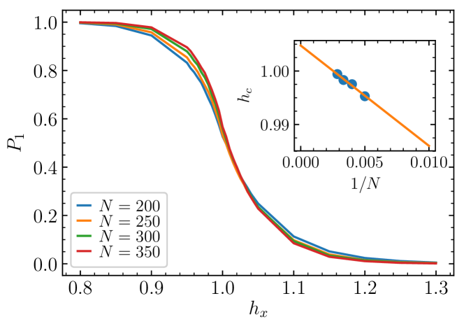
In the limit of the transverse field strength, $h_{x}\rightarrow 0$ we have a ferromagnetic phase while in the the limit of $h_{x}\rightarrow\infty$ we have a paramagnetic phase. The errors corresponding to the ferromagnetic phase are given by observing the neighbors, i.e., neighbors with different (same) parity indicate the presence (absence) of a domain-wall (error). While the errors of the ferromagnetic phase are different than in the antiferromagnetic case, their correlations are identical as the ferromagnetic Ising model can be mapped onto the antiferromagnetic one by a unitary transformation flipping every second spin. In Fig. 6, we confirm the expectation that the transition between the ferromagnet and the paramagnet can be detected by a DNN trained on the antiferromagnetic case.

V.2 Detecting intrinsic topological order in perturbed punctured toric code

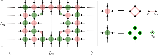
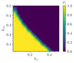
In this section, we consider a case where the two models are not connected by a unitary transformation. Here, we start from a DNN trained on the errors of a perturbed planar toric code with rough boundaries and apply it to a punctured toric code containing a hole in the center, see Fig. 7a. Additionally, on every second plaquette, we change the perturbation from a local magnetic field $h_{x}\sigma_{x}^{i}$ to a ferromagnetic Ising interaction $h_{xx}\sigma_{x}^{i}\sigma_{x}^{j}$. A puncture in the toric code is realized by turning off either the $B_{p}$ or $A_{v}$ interactions. In the current scenario, we turn off the $B_{p}$ interactions over a small region resulting in a puncture. The topological phase corresponding to the punctured toric code is different from that of the nonpunctured toric code as the former has a degenerate ground state manifold while the latter is nondegenerate. However, it is still possible to map out the phase diagram of the punctured toric code in the presence of perturbation by using a DNN trained on the errors of the toric code with no punctures, as shown in Fig. 7. For the purpose of predicting the phase diagram of the perturbed punctured toric code, we consider that the punctured faces do not host any errors. However, it is important to note that the above technique of estimating the phase diagram of the punctured toric code with a DNN trained on errors of nonpunctured toric code is appropriate only in the limit where few (in comparison to the total system size) interactions are turned off.

VI Summary and Discussion

In summary, we have introduced a novel machine learning based classifier to detect gapped quantum phases. Our method enhances the operational definition to not only detect gapped quantum phases with topological order but also other quantum phases with local order. Furthermore, within the machine learning approach, it is no longer necessary to construct appropriate error correction algorithms, as this task is effectively carried out by a deep neural network (DNN). Our work establishes a correspondence between gapped quantum phases and their errors along with the correlations between them. In other words, any gapped quantum phase can be uniquely identified and quantified by its errors on top of a suitable reference state and the correlations between them. Crucially, the DNN trained with a certain perturbation can also successfully detect the quantum phase and its boundaries in the presence of different perturbations.

Future avenues of our machine learning approach include (a) exploring quantum phases in an open quantum system with a DNN trained on the errors in a closed quantum system, (b) exploring other DNN training routines like using random unitaries coupled with random measurements and/or random dissipative channels, (c) quantifying the time evolution of a quantum system out of equilibrium using machine learning classifiers. As a further development of the method, autoencoders could potentially be used to deduce the excitation basis and therefore the errors associated with a given gapped quantum phase. Hence, autoenconders in combination with DNNs could lead to a powerful framework for the classification of any gapped phase in the framework of machine learning. Furthermore, recent technological progress has enabled the possible realization of topological states of matter in quantum simulation architectures Semeghini et al. (2021); Satzinger et al. (2021), but unambigious identification of topological order remains challenging because of the exponential resources required to measure quantities like the topological entanglement entropy Kitaev and Preskill (2006); Levin and Wen (2006). In this context, our machine learning approach can be used to verify the existence of topological order in these experiments in an efficient way.

Appendix A Machine Learning parameters for learning the error correlations

In this appendix, we provide details on the neural networks employed to train the errors associated with gapped quantum phases. As introduced earlier and as depicted in Fig. 1, we consider a DNN with input as the errors, multiple hidden layers and two outputs. For a given system size, there is a fixed number of errors which thereby fixes the input nodes to the DNN. Each hidden layer has approximately half the number of nodes as the previous layer and the number of hidden layers is increased until the nodes in the hidden layers are less than 30, with the final output layer having two nodes. Having detailed the architecture, we briefly comment on the tools used to construct the neural networks, as well as the training parameters employed. We have implemented the above DNN architecture using FluxML Innes et al. (2018), a machine learning library in Julia. For training purposes, we choose the cross entropy loss function with the Adam algorithm for optimization. Further, we set the learning rate, $\eta$, on the order of $10^{-3}$, and have used GPUs for the purpose of training. For training and predicting purposes, we generate around 25,000 error samples for a given wavefunction.

Appendix B Error correction circuit used to compute the correction time statistics

In this appendix, we briefly review the error correction circuit employed to compute the standard deviation of the circuit depth used within the operational definition as shown in Fig. 5. For a given wavefunction, we sample the errors as outlined in the main text and for each error sample we perform the error correction until all the face excitations are annihilated. To compute the error correction time for a given error sample, we follow the procedure from Ref. Jamadagni and Weimer, 2020 and attach to each error a walker that traverses the surrounding in a diamond shaped pattern of increasing Manhattan distance from the error. Whenever two walkers start to overlap, their corresponding errors are fused and removed from the system. The circuit depth of a particular error sample is then given by the number of steps required until the last errors have been fused.

References

- Landau (2008) L. Landau, On the Theory of Phase Transitions, Ukr. J. Phys. 53, 25 (2008), originally published in Zh. Eksp. Teor. Fiz. 7, 19–32 (1937).
- Carrasquilla and Melko (2017) J. Carrasquilla and R. G. Melko, Machine learning phases of matter, Nature Physics 13, 431–434 (2017).
- Beach et al. (2018) M. J. S. Beach, A. Golubeva, and R. G. Melko, Machine learning vortices at the Kosterlitz-Thouless transition, Phys. Rev. B 97, 045207 (2018).
- Dong et al. (2019) X.-Y. Dong, F. Pollmann, and X.-F. Zhang, Machine learning of quantum phase transitions, Physical Review B 99 (2019).
- Zhang et al. (2017) Y. Zhang, R. G. Melko, and E.-A. Kim, Machine learning quantum spin liquids with quasiparticle statistics, Phys. Rev. B 96, 245119 (2017).
- Zhang and Kim (2017) Y. Zhang and E.-A. Kim, Quantum Loop Topography for Machine Learning, Phys. Rev. Lett. 118, 216401 (2017).
- Broecker et al. (2017) P. Broecker, J. Carrasquilla, R. G. Melko, and S. Trebst, Machine learning quantum phases of matter beyond the fermion sign problem, Scientific Reports 7 (2017).
- Huang et al. (2021) H.-Y. Huang, R. Kueng, G. Torlai, V. V. Albert, and J. Preskill, Provably efficient machine learning for quantum many-body problems, arXiv:2106.12627 (2021).
- Carleo and Troyer (2017) G. Carleo and M. Troyer, Solving the quantum many-body problem with artificial neural networks, Science 355, 602–606 (2017).
- Deng et al. (2017a) D.-L. Deng, X. Li, and S. Das Sarma, Machine learning topological states, Physical Review B 96 (2017a).
- Deng et al. (2017b) D.-L. Deng, X. Li, and S. Das Sarma, Quantum Entanglement in Neural Network States, Phys. Rev. X 7, 021021 (2017b).
- Biamonte et al. (2017) J. Biamonte, P. Wittek, N. Pancotti, P. Rebentrost, N. Wiebe, and S. Lloyd, Quantum machine learning, Nature 549, 195–202 (2017).
- Cong et al. (2019) I. Cong, S. Choi, and M. D. Lukin, Quantum convolutional neural networks, Nature Physics 15, 1273–1278 (2019).
- Beer et al. (2020) K. Beer, D. Bondarenko, T. Farrelly, T. J. Osborne, R. Salzmann, D. Scheiermann, and R. Wolf, Training deep quantum neural networks, Nature Communications 11 (2020).
- Beer et al. (2021) K. Beer, M. Khosla, J. Köhler, and T. J. Osborne, Quantum machine learning of graph-structured data, arXiv:2103.10837 (2021).
- Jamadagni and Weimer (2020) A. Jamadagni and H. Weimer, An Operational Definition of Topological Order, arXiv:2005.06501 (2020).
- Jamadagni and Weimer (2021) A. Jamadagni and H. Weimer, Error-correction properties of an interacting topological insulator, arXiv:2103.00011 (2021).
- van Nieuwenburg et al. (2017) E. van Nieuwenburg, Y.-H. Liu, and S. Huber, Learning phase transitions by confusion, Nature Physics 13, 435 (2017).
- Fishman et al. (2020) M. Fishman, S. R. White, and E. M. Stoudenmire, The ITensor Software Library for Tensor Network Calculations, arXiv:2007.14822 (2020).
- Han et al. (2018) Z.-Y. Han, J. Wang, H. Fan, L. Wang, and P. Zhang, Unsupervised Generative Modeling Using Matrix Product States, Phys. Rev. X 8, 031012 (2018).
- Ovchinnikov et al. (2003) A. A. Ovchinnikov, D. V. Dmitriev, V. Y. Krivnov, and V. O. Cheranovskii, Antiferromagnetic Ising chain in a mixed transverse and longitudinal magnetic field, Phys. Rev. B 68, 214406 (2003).
- Elben et al. (2020) A. Elben, J. Yu, G. Zhu, M. Hafezi, F. Pollmann, P. Zoller, and B. Vermersch, Many-body topological invariants from randomized measurements in synthetic quantum matter, Science Adv. 6, eaaz3666 (2020).
- Wen (2019) X.-G. Wen, Choreographed entanglement dances: Topological states of quantum matter, Science 363, eaal3099 (2019).
- Chen et al. (2010) X. Chen, Z.-C. Gu, and X.-G. Wen, Local unitary transformation, long-range quantum entanglement, wave function renormalization, and topological order, Phys. Rev. B 82, 155138 (2010).
- Su et al. (1980) W. Su, J. Schrieffer, and A. Heeger, Soliton excitations in polyacetylene, Phys. Rev. B 22, 2099 (1980).
- Kitaev (2003) A. Y. Kitaev, Fault-tolerant quantum computation by anyons, Ann. Phys. (N. Y.) 303, 2 (2003).
- Beigi et al. (2011) S. Beigi, P. W. Shor, and D. Whalen, The Quantum Double Model with Boundary: Condensations and Symmetries, Commun. Math. Phys. 306, 663 (2011).
- Semeghini et al. (2021) G. Semeghini, H. Levine, A. Keesling, S. Ebadi, T. T. Wang, D. Bluvstein, R. Verresen, H. Pichler, M. Kalinowski, R. Samajdar, A. Omran, S. Sachdev, A. Vishwanath, M. Greiner, V. Vuletić, and M. D. Lukin, Probing topological spin liquids on a programmable quantum simulator, Science 374, 1242 (2021).
- Satzinger et al. (2021) K. J. Satzinger, Y.-J. Liu, A. Smith, C. Knapp, M. Newman, C. Jones, Z. Chen, C. Quintana, X. Mi, A. Dunsworth, C. Gidney, I. Aleiner, F. Arute, K. Arya, J. Atalaya, R. Babbush, J. C. Bardin, R. Barends, J. Basso, A. Bengtsson, A. Bilmes, M. Broughton, B. B. Buckley, D. A. Buell, B. Burkett, N. Bushnell, B. Chiaro, R. Collins, W. Courtney, S. Demura, A. R. Derk, D. Eppens, C. Erickson, L. Faoro, E. Farhi, A. G. Fowler, B. Foxen, M. Giustina, A. Greene, J. A. Gross, M. P. Harrigan, S. D. Harrington, J. Hilton, S. Hong, T. Huang, W. J. Huggins, L. B. Ioffe, S. V. Isakov, E. Jeffrey, Z. Jiang, D. Kafri, K. Kechedzhi, T. Khattar, S. Kim, P. V. Klimov, A. N. Korotkov, F. Kostritsa, D. Landhuis, P. Laptev, A. Locharla, E. Lucero, O. Martin, J. R. McClean, M. McEwen, K. C. Miao, M. Mohseni, S. Montazeri, W. Mruczkiewicz, J. Mutus, O. Naaman, M. Neeley, C. Neill, M. Y. Niu, T. E. O’Brien, A. Opremcak, B. Pató, A. Petukhov, N. C. Rubin, D. Sank, V. Shvarts, D. Strain, M. Szalay, B. Villalonga, T. C. White, Z. Yao, P. Yeh, J. Yoo, A. Zalcman, H. Neven, S. Boixo, A. Megrant, Y. Chen, J. Kelly, V. Smelyanskiy, A. Kitaev, M. Knap, F. Pollmann, and P. Roushan, Realizing topologically ordered states on a quantum processor, Science 374, 1237 (2021).
- Kitaev and Preskill (2006) A. Kitaev and J. Preskill, Topological Entanglement Entropy, Phys. Rev. Lett. 96, 110404 (2006).
- Levin and Wen (2006) M. Levin and X.-G. Wen, Detecting Topological Order in a Ground State Wave Function, Phys. Rev. Lett. 96, 110405 (2006).
- Innes et al. (2018) M. Innes, E. Saba, K. Fischer, D. Gandhi, M. C. Rudilosso, N. M. Joy, T. Karmali, A. Pal, and V. Shah, Fashionable Modelling with Flux, CoRR abs/1811.01457 (2018).