High-Precision Redshifts for Type Ia Supernovae with the Nancy Grace Roman Space Telescope P127 Prism
Abstract
We present results from simulating slitless spectroscopic observations with the Nancy Grace Roman Space Telescope’s (Roman) Wide-Field Instrument (WFI) P127 prism spanning 0.75 to 1.8 . We quantify the efficiency of recovered Type Ia supernovae (SNe Ia) redshifts, as a function of P127 prism exposure time, to guide planning for future observing programs with the Roman prism. Generating the two-dimensional dispersed images and extracting one-dimensional spectra is done with the slitless spectroscopy package pyLINEAR along with custom-written software. From the analysis of 1698 simulated SN Ia P127 prism spectra, we show the efficiency of recovering SN redshifts to , highlighting the exceptional sensitivity of the Roman P127 prism. Redshift recovery is assessed by setting a requirement of . We find that 3 hr exposures are sufficient for meeting this requirement, for of the sample of mock SNe Ia at and within days of rest-frame maximum light in the optical. We also show that a 1 hr integration of Roman can achieve the same precision in completeness to a depth of AB mag (or ). Implications for cosmological studies with Roman P127 prism spectra of SNe Ia are also discussed.
1 Introduction
The Nancy Grace Roman Space Telescope (Roman) will, through its core community High Latitude Time Domain Survey (HLTDS), observe on the order of Type Ia supernovae (SNe Ia; e.g., Hounsell et al., 2018; Akeson et al., 2019). Most of these SNe will be within redshifts , and are required to be observed with sufficient depth per epoch to enable accurate measurements of dark energy properties that significantly improve the dark energy figure of merit (FoM; Spergel et al., 2015; Hounsell et al., 2018). To accomplish these goals, the two Supernova Science Investigation Teams (SITs) have provided a jointly recommended reference survey in Rose et al. (2021).
An important assumption in Rose et al. (2021) is that the redshifts for all SNe Ia (or host galaxies) are well measured, i.e., on the order of a tenth of a percent, and it is assumed that Roman spectroscopic elements will be used as a part of the Roman HTLDS strategy to obtain those redshifts. The Roman Wide-Field Instrument (WFI), with a field-of-view of 0.281 deg2, is expected to have two slitless-spectroscopy spectral elements: a low-resolution prism (P127; –170; ) and a slightly higher-resolution grism (G150; –865; ).111 https://roman.gsfc.nasa.gov/science/WFI_technical.html provides more complete details on the current Roman WFI design. Compared to the grism, the Roman prism, while lower resolution, is mag more sensitive than the Roman grism for a 1 hr exposure making it better suited for analysis of fainter SNe with broad absorption features (Table 1).
As part of the SIT effort, the primary objective of this work is to evaluate the utility of the prism spectra, particularly the influence of the exposure time on the signal-to-noise ratio (S/N) and redshift accuracy. These results are needed to optimize the spectroscopic component of the HLTDS and future observations with the Roman prism. Current estimates for the HLTDS design involve some (as yet undecided) combination of prism-to-imaging time, along with coaddition of spectra taken from multiple visits, as well as time series analysis (Saunders et al., 2018). Based on estimates of current Roman WFI/P127 capabilities, we provide here a base platform from which future considerations of prism exposures for the HLTDS can continue, while also giving a broader context for other programs that involve the Roman prism. We analyze the redshift recovery for a single long-exposure visit (which can still include multiple position angles) where all data for a given SN Ia are taken such that spectral or luminosity variations can be neglected (over the timescale of the visit).
With simulated broadband filter images of a single Roman HLTDS pointing (hereafter referred to as direct images) in the WFI/F106 filter as input (Wang et al., 2022), our approach involves simulating two-dimensional (2D) spectroscopic images (dispersed images) through the Roman prism, and analyzing the extracted one-dimensional (1D) spectra, as will be done for real Roman data. This paper focuses primarily on the recovery of SN Ia redshifts, although our fitting pipeline also attempts to constrain SN Ia phase (relative to peak) and dust extinction along the line of sight. The simulation products and the associated codes will be publicly available at the IPAC-hosted simulations page222https://roman.ipac.caltech.edu/sims/Simulations_csv.html and GitHub333https://github.com/bajoshi/roman-slitless, respectively. Future papers will focus on recovery of (a) other SN Ia properties (e.g., Si II velocities) while also including coadded shorter exposures from multiple visits at different phases such that the SN brightness and spectral evolution are measured, (b) deblending of SN Ia and host galaxy spectra, and (c) (host-)galaxy stellar-population parameters from their prism spectra.
This work is structured as follows: § 2 goes into details of the simulation and analysis methods, § 2.1 discusses the models used for SNe Ia, galaxies, and stars; § 2.2 describes how host galaxy light and SN light are blended for SNe that overlap with their host galaxy in our simulation; § 2.3 and § 3.1 provide an overview of the pyLINEAR package used to simulate the 2D dispersed images and extract the 1D spectra; and § 3.2 describes the fitting process applied to the extracted 1D spectra. Finally, § 4 discusses the results obtained from our fitting pipeline, particularly with regards to the efficiency of recovering redshifts. The cosmological model assumed in this paper is flat with and H km s-1 Mpc-1, and all magnitudes are in the AB system (Oke & Gunn, 1983).
2 Simulation and Analysis Methods
Redshifts and distance moduli are the two independently-measured quantities for SNe Ia that allow astronomers to constrain cosmological models. Our goal here is to analyze the accuracy of redshifts recovered from simulated 1D P127 spectra of SNe Ia, while keeping the simulation as realistic as possible. A schematic of the simulation pipeline, as well as the inputs and products, is shown in Figure 1.
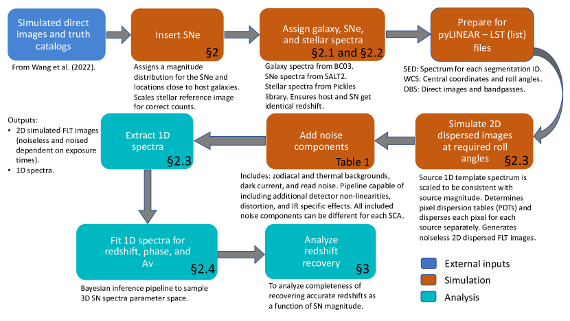
Our process consists of the following steps which includes an end-to-end simulation (steps i and ii) and analysis of the simulation products (steps iii and iv):
- (i)
-
(ii)
generate dispersed images at required roll angles and exposure times for the Roman WFI/P127 prism, (§ 2.3)
-
(iii)
extract 1D slitless spectra of all detected sources (§ 3.1), and
-
(iv)
recovery of SNe Ia and galaxy stellar population parameters through a Markov Chain Monte Carlo (MCMC; § 3.2) fitting of the “observed” slitless spectroscopy.
The simulation is based on one pointing, of all 18 WFI detectors, generated at three roll angles with total exposure times of 1200, 3600, and 10,800 s. The roll angles we use are 0∘, 70∘, and 140∘, measured east of north. The exposure times are built up by adding repeated observations assuming that the longest individual exposure is limited to 900 seconds. Given that detector-specific details are not yet known for Roman, our code runs the simulation on a single detector and repeats the simulation 18 times with a different scene on the sky each time (where “scene” is defined by the shapes, sizes, locations, and brightness for all objects within the field-of-view). We also limit the number of randomly-inserted SNe into each detector to a range of (i.e., % of total sources which are typically ), so as to not artificially introduce excessive spectral overlap. In total, our simulation contains 1698 SNe Ia.
| Optics/Detector characteristic | HST WFC3/IR grisms | Roman WFI | ||
|---|---|---|---|---|
| G102 | G141 | P127 | G150 | |
| Dark current [/pix/s] | 0.05 | 0.05 | 0.0015 | 0.0015 |
| Read noise [ rms] | ||||
| Zodiacal background [/pix/s] aaThe zodiacal light estimates for the HST grisms vary primarily with Sun angle and time of year (Pirzkal & Ryan, 2020). We therefore use median values for the distribution of zodiacal light levels for the HST grisms. Assumes a 1.1 factor for zodiacal light for Roman (private communication, Jeffrey Kruk) which is expected to depend on Galactic latitude. | 0.48 | 1.04 | 1.047 | 1.047 |
| Thermal background [/pix/s] | 0.02 | 0.02 | 0.064 | 0.064 |
| 1 hr limiting magbbFor the HST grisms, limiting magnitude is defined as 5 per continuum pixel in the and bands for G102 and G141, respectively (Kuntschner et al., 2010). For the Roman prism and grism, limiting magnitude is defined as per 2 pixel resolution element in the continuum, at 1.2 m, for a point source. | 22.6 | 22.9 | 23.5 | 20.5 |
| Resolution [] | 70–170 | 435–865 | ||
| Wavelength coverage [nm] | 800–1150 | 1075–1700 | 750–1800 | 1000–1930 |
Note. — A comparison of relevant properties of the HST WFC3 IR grisms and the Roman prism and grism, some of which factor into the increased sensitivity of the Roman prism. See https://roman.gsfc.nasa.gov/science/WFI_technical.html and https://wfirst.ipac.caltech.edu/sims/Param_db.html, for details on WFI detector performance. See https://www.stsci.edu/hst/instrumentation/wfc3/documentation/grism-resources for details on the HST WFC3 grisms. Since the grisms have multiple orders, relevant quantities are quoted here for the +1 order.
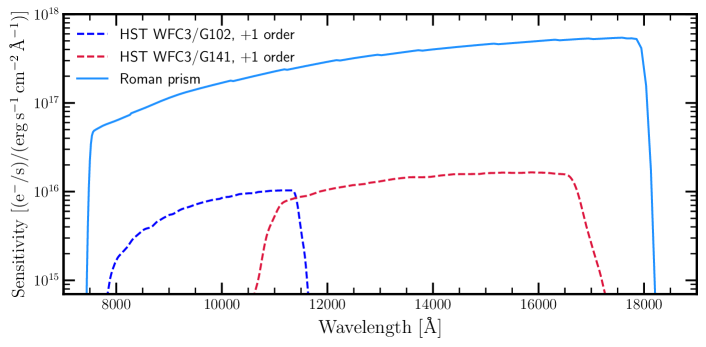
Simulating the photoelectron count rate for a given source observed through the Roman prism requires use of the sensitivity curve (Figure 2) along with (i) the counts for each pixel associated with the source in the direct image, (ii) a description of the spectral trace for the Roman prism, (iii) a spectrum associated with each source pixel, and (iv) the noise characteristics of the instrumentation (see noise budget components in Table 1). The spectral trace is defined as the location of the centroid of the spectrum along the spatial direction (see e.g., Kümmel et al., 2009; Pirzkal et al., 2016). Table 1 shows a comparison of properties between the Hubble Space Telescope (HST) Wide Field Camera 3 (WFC3) infrared (IR) grisms and the Roman prism and grism. Table 1 also shows the noise terms included in our simulation. However, it does not include IR detector-specific effects, such as flux-dependent sensitivity and interpixel capacitance, which we expect to have a smaller effect on the prism spectra compared to the terms already included. This table also shows that the primary reason for preferring the Roman prism over the grism for observing SNe Ia is the mag deeper sensitivity of the prism, which is particularly helpful for estimating redshifts to fainter SNe Ia given the broad absorption features typical of SN Ia spectra. Another significant reason for the increased sensitivity of the Roman prism is the lack of dispersion orders. Since the grisms disperse light into multiple orders and the prism disperses light into a single order, the grisms lose a significant fraction of the available light; typically only the +1 order spectrum from a grism is analyzed given that gratings are blazed to maximize throughput to the +1 order.
Figure 2 shows a comparison between the sensitivities of the Roman prism and HST WFC3 IR grisms G102 and G141. According to current best estimates of sensitivity, the Roman prism is a factor of more sensitive than HST/WFC3 IR grisms at all wavelengths covered by the HST grisms. The prism’s performance is expected to result in per pixel in a 1 hr exposure of a point source with = 23.5 mag AB444https://roman.gsfc.nasa.gov/instruments_and_capabilities.html (although we recover per pixel from analyzing our simulations).
2.1 Stellar Population and SALT2 Models
Prior to dispersing the simulated direct images we assign each source in the direct images a model spectrum. Briefly, the simulated direct images contain stars and galaxies and while they also contain SNe Ia, the rates employed result in too few SNe for our analysis (for more details we refer the reader to Wang et al. 2022 and references therein).
Therefore, we begin by overlaying additional SNe into the direct images as point sources. Typical SNe Ia simulations begin by selecting a random redshift from a rate model, and then computing SN Ia model magnitudes at each phase. To simulate an appropriate magnitude range, we simulate with a different approach in which random magnitudes are chosen in the range , and the corresponding redshift is determined for each magnitude (corresponding to SNe Ia approximately within ). We overlay the SNe into the direct images with a synthetic apparent magnitude chosen first instead of choosing a redshift first and then letting the apparent magnitude be decided by the cosmology, SN Ia phase, and line of sight dust attenuation. This approach is motivated by the need to acquire a large enough sample of fainter SNe, because we expect the accuracy of inferred redshifts to deteriorate for fainter SNe, while still completing the simulations within a realistic time-frame, owing to the computationally expensive nature of the simulations. Choosing the apparent magnitude first allows us to have a well-known magnitude distribution for the overlaid SNe Ia. For the SN Ia model template, we employ an extension of the SALT2 SN Ia model that extends into the near-IR (Guy et al., 2007; Pierel et al., 2018). This model provides rest-frame SN Ia spectra from 1700 Å to 2.5 m, and with phases days to days relative to optical peak. The SALT2 model employed here is a fiducial model, i.e., it assumes . While this model does not fully capture the diversity in SNe Ia, it still serves our main purpose of the assessing the redshift recovery for a typical SN Ia at any given redshift. This work is largely focused on analyzing how the S/N affects redshift recovery, for which our model for an average SN Ia at each redshift appears sufficient (see § 3.2 and the discussion in § 4). The diversity of SNe Ia and the analysis of other SN Ia subtypes, which are known to have variable intrinsic brightness and different spectral features (e.g., 91bg or 91T), will be addressed in a future work.
The probability distribution function (PDF) for the magnitude distribution follows a power law ( with ), ensuring a distribution of SN magnitudes that allows for a slightly larger number of fainter SNe for analysis. To obtain a statistically significant sample of SNe Ia for analysis we insert a relatively large number of SNe into each detector (as previously mentioned SNe per detector). While this rate model is not consistent with the number density of SNe that will be observed in a single visit, our decision is again driven by the need to obtain a large number of SN prism spectra for analysis. Each SN is assigned a spectrum with a randomly chosen phase within days from peak. Next, we apply dust extinction following the Calzetti et al. (2000) law, chosen from mag, with an exponentially declining PDF weighted in favor of lower values ( with ), in order to simulate realistic dust extinction from local environments of SNe, following Jha et al. (1999) and Holwerda et al. (2015). Finally, we apply cosmological redshift to the inserted SN spectrum by redshifting the wavelength grid and scaling the spectrum flux so that the synthetic magnitude matches the already assigned SN magnitude.
For (host-) galaxies we use the Bruzual & Charlot (2003) GALAXEV library of stellar-population models. Each galaxy is assigned a composite stellar population with a delayed- star-formation-rate (SFR) model (SFR ) for the star-formation history, along with a stellar mass of , a redshift of (if it is an SN host galaxy, then the SN and host are assigned the same redshift), and finally a dust extinction with randomly chosen from mag. For Galactic stellar point sources in the images we assign spectra from the Pickles stellar library, that provide stellar spectra from 1150 Å to 25,000 Å (Pickles, 1998). The Pickles library provides 131 flux-calibrated stellar templates for stellar types within the range O5–M2, with the stellar type being chosen randomly in our simulations.
2.2 Blending of host galaxy and Supernova Light
A significant advantage of slitless spectroscopy is the ability to obtain a spectrum for all objects within the field-of-view (FoV). This also introduces significant data-reduction challenges, particularly with disentangling spectra from objects that are very close to each other and/or lie along the dispersion direction such that their spectra overlap. In traditional slitless spectroscopy parlance, the term contamination usually refers to the unwanted overlap of one or more spectra on the spectrum of the object of interest. Generally this effect can be mitigated by taking data at multiple roll angles so that there is at least one roll angle within which the spectrum of interest contains little to no contamination.
In the specific case of slitless spectroscopic observations of an SN Ia and its host galaxy, an additional concern is the blending of light from the host galaxy and the SN — that is, within pixels that overlap between the SN and its host galaxy, the total flux (and therefore the spectrum from that pixel) is a combination of host and SN. This introduces a minimum floor of contamination (referred to as blending below to distinguish from the traditional notion of contamination) that will be present in all observations of the SN Ia regardless of the roll angle. This situation is analogous to that of taking slitless spectra of a galaxy containing one or more star-forming knots — in this case, the underlying galaxy spectrum is blended with the emission-line spectrum of the star-forming region.
In order to represent this effect within our simulations, for each SN source that has an overlap between the host galaxy and SN we carry out the following steps.
(1) For each overlapping pixel , the effective spectrum from the pixel is given by
| (1) |
where and denote linear combination coefficients, and and are the spectra of the host galaxy and SN, respectively. The coefficients and are fractions of the total counts within a pixel that belong to the host galaxy and SN, respectively. We also make the simplifying assumption (for all sources) that the input spectrum remains constant over the spatial extent of the source.
(2) The final spectrum of the SN containing overlap with the host is given by a weighted sum of the spectra from overlapping pixels (i.e., blended SN and host spectra) and non-overlapping pixels (i.e., pure SN Ia spectra):
| (2) |
where is the final blended spectrum of the SN and () denote (non-)overlapping pixels. The indices, i and j, sum over SN pixels that overlap and do not overlap with the host galaxy, respectively. The weights and are computed to ensure that the relative flux contribution from each pixel toward the “effective” source count, which includes both host galaxy and SN counts, is reflected in the final spectrum. This final blended spectrum becomes the effective 1D spectral template for the SN, i.e., each pixel associated with the SN, in the segmentation map, is assigned the spectrum . The effective 1D spectral template is then passed to pyLINEAR for simulating 2D dispersed images as described in § 2.3.
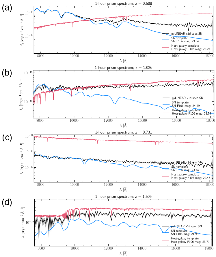
Figure 3 shows examples of blended SN Ia and host galaxy spectra. Extracted spectra (the extraction process is described in § 3.1) are effectively the weighted sum of the SN and host input templates (Equation 2). The extent of blending depends on the number of pixels that overlap between the SN and host galaxy, the exposure time, and their brightness relative to each other. Without any attempt to deblend the host galaxy spectrum from the SN spectrum, our automated fitting pipeline (described in § 3.2) fails to recover the SN redshift in each of the cases shown here. Overall, 54% of the SNe Ia in our simulation are affected, to varying degrees, by blended host galaxy light. We arrive at this fraction by counting any SN in our simulation that has one or more pixels that overlap with the host galaxy. This “blended” fraction is affected by the placement of the SNe which in our case is at the vertices of the “bounding box” of the segmentation pixels of the host galaxy. This effectively simulates placing the SNe Ia at the effective light radius of the host galaxy. This placement choice avoids completely overwhelming the SN light by the host galaxy light while still allowing a significant fraction of SNe to contain blended light for later analysis.
In practice, for dark energy studies, SNe Ia that are deeply embedded in host galaxy light would be rejected (if the host light cannot be reliably subtracted) so that they do not affect the inference of cosmological parameters. The total number of SNe Ia expected within the Roman cosmological sample has already estimated by various other studies (; e.g., Hounsell et al. (2018); Akeson et al. (2019)). With regards to host galaxy blended light this sample size will depend on the strictness of any selection cuts for blended host light and the success of any algorithms used to deblend host galaxy light which are being developed for Roman. We therefore do not expect that inferred cosmological parameters will significantly depend on the amount of blended host galaxy light, however their statistical errors which depend on the sample size will be affected.
2.3 Simulation of 2D dispersed images
Here we provide a brief overview of the process to simulate 2D dispersed images carried out by pyLINEAR. For a detailed explanation of the pyLINEAR algorithm, the reader is referred to Ryan et al. (2018a, b).
The driving motivations for the algorithm behind pyLINEAR are to employ dispersed data from multiple roll angles to optimally handle spectral contamination due to overlapping spectra, and also to extract spectra with the optimal spectral resolution without sacrificing the S/N. pyLINEAR simulates 2D dispersed images by dispersing 1D high-resolution model spectral templates for each pixel associated with each source in the direct image. It requires a description of the scene on the sky and a description of the spectral trace and sensitivity of the dispersing element being considered.
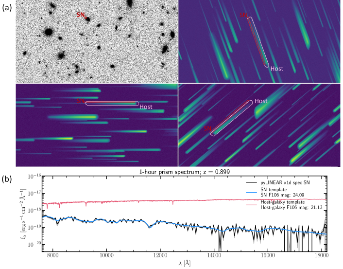
We modify pyLINEAR defaults to allow the simulation of prism exposures in which the dispersion is strongly dependent on wavelength. Briefly, traditional slitless spectroscopy routines (e.g., aXe, Kümmel et al. 2009; pyLINEAR) describe the spectral trace with a polynomial that is parameterized by the path length along the trace. For describing the spectral trace of the Roman prism, we build on the foundation of the generalized 2D polynomials introduced by Pirzkal & Ryan (2017). These polynomials are a function of the and coordinates on the dispersed image and another parameter (which spans and can generally, although not always, be identified with wavelength coverage). One of the quantities required to be computed in simulating 2D spectra is the wavelength . For most grisms, this is a first-order equation in . To allow for a variable dispersion with wavelength relation, however, we had to change this to a second-order equation in . This change is nontrivial because the polynomial relation must also be inverted to solve for the coefficients of that give the known dispersion vs. wavelength relation. For readers interested in simulating Roman prism spectra, the configuration file for aXe and pyLINEAR is available from the corresponding author. Figure 4 shows an example of simulated 2D dispersed images through the Roman prism and the extracted SN spectrum from a SN and its host galaxy.
3 Analysis of simulation products
3.1 Extraction of 1D spectra
The extraction of 1D spectra, which involves solving for the flux at each wavelength for each source, is an overconstrained problem that has more data values than unknown parameters — that is, the set containing observed information (direct and dispersed images) is far larger than the set of information to be solved for (fluxed spectra for all objects). pyLINEAR attempts to solve for the set of spectra that simultaneously satisfy all the available dispersed data (i.e., all roll angles and dithers). pyLINEAR defines the system of linear equations that connect the observed data and the unknown fluxes and recasts to a known linear-algebra problem with sparse matrices, . Roughly, elements in the matrices and represent the observed counts and the weighting coefficients that transform them into the fluxed spectra, and represents the unknown vector of fluxed spectra for all objects. This amounts to finding a minimum in the equation,
| (3) |
However, if the matrix has noise (which real data does), then the solution to equation 3 is numerically unstable. Therefore, the actual equation to be solved is modified to the following regularized least squares equation,
| (4) |
where, is the regularization parameter (see Ryan et al. 2018a for more details on the regularization). pyLINEAR employs the LSQR (Paige & Saunders, 1982) algorithm for solving the above equation with large sparse matrices.
In contrast to aXe (Kümmel et al., 2009), which provides a separate spectrum per object for each roll angle, while leaving the combining of spectra at different roll angles to the user, pyLINEAR provides a single extracted 1D spectrum per object given its algorithmic philosophy of solving for the optimal flux vector that satisfies all the available data. Effectively, the combining of the spectra at different roll angles is done internally within pyLINEAR. This approach naturally handles the problem of overlapping spectra without leaving the contamination subtraction as a separate analysis task. Additionally, pyLINEAR has the advantage of achieving better spectral resolution without sacrificing the S/N in the extracted spectrum.
3.2 Parameter Recovery through Bayesian Inference
Extracted 1D spectra are fit for redshift, phase, and dust extinction. It is important to note that we do not fit SALT2 light curve parameters here, and . We only fit for the parameters which are typically inferred from spectroscopic data, i.e., redshift, whereas fitting for light curve parameters, at present, requires photometric data.555In the future, it should be more viable to fit for and from spectral features (e.g., Mandel et al., 2014; Zhao et al., 2021). Cosmological inference should not be affected by the lack of fitting for and , given that redshift is an independent measure needed for the Hubble diagram. The fitting is done with the Python package emcee (Foreman-Mackey et al., 2013, 2019), which samples the 3-dimensional (3D) posterior space for SNe models. Our automated fitting pipeline uses 500 walkers and 1000 steps. The walkers use the default “stretch-move” within emcee for sampling the posterior. We start the walkers at the optimal position indicated by the approximate global minimum. The minima for the walkers’ starting location is found by doing a brute force evaluation for each model on a coarse grid of redshift ( within [0.01, 3.0]), phase ( within [, 50]), and dust extinction ( mag within [0.0, 3.0] mag). We employ flat priors on SN phase and dust extinction () with the following ranges: and . For the SN redshift we employ a broad Gaussian prior with a mean of 1.2 and a standard deviation of 0.7. The broad Gaussian redshift prior allows down-weighting of very low- and high- SNe (while not rejecting them outright). Finally, we require S/N3 for the extracted 1D spectrum prior to fitting. This S/N is computed for the entire prism spectrum using the DER-SNR algorithm of Stoehr et al. (2008).
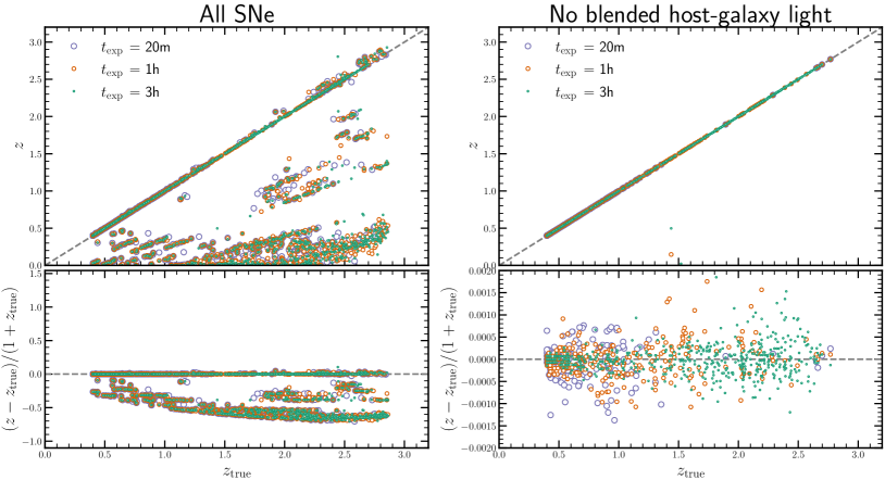
Figure 5 shows the recovery of SN Ia redshifts for all SNe in the simulation (left column) and for the subset without host galaxy light (right column). The recovery plots for phases and dust attenuation are shown in the appendix (Figure 8). As expected, longer exposure times provide the most accurate inferred quantities. Most of the failed estimates of redshift are caused by host galaxy light blending with SN light. As shown in Figure 5, the inferred redshifts are systematically underestimated for SNe whose spectra contain light from the host galaxy, given that these failures are absent in the plot that ignores SNe which contain blended host galaxy light. The failures generally come from three modes. First, the continuum slope of the host galaxy spectrum, when blended with the typically fainter SN spectrum, causes a mismatch between SNe Ia absorption features. This mismatch is driven by the continuum slope of the host galaxy at the red end which dominates the in the SED fitting. The necessity for the fitting pipeline to match the host galaxy continuum slope (instead of the SN continuum slope) pushes the pipeline estimate to underestimated redshifts (and also younger phases, Figure 8). Second, strong host galaxy absorption features (e.g., 4000 Å/Balmer breaks) are misidentified by the fitting pipeline with SN absorption features. This is shown by the clear linear feature below the 1:1 line. Lastly, the cluster of failures at the bottom of the figure are cases where host galaxy light dominates the extracted 1D spectrum. However, it is worth recalling that the redshift estimates in Figure 5 come from fitting only the SNe spectra, and that a host galaxy spectrum can always be observed after the SN light has faded allowing for a clean subtraction (and also allowing for a redshift estimate directly from the host galaxy spectrum in some cases).
In this work, we do not attempt to deblend host galaxy and SN light. Our fitting pipeline proceeds on the assumption that there is no host galaxy light blended into the SN Ia spectrum, and it fits the SN Ia spectrum without any attempt to subtract the host galaxy spectrum. We leave this deblending to a future work which will likely involve marginalizing over nuisance parameters that describe the host galaxy spectrum.
4 Redshift Efficiency Dependence on Exposure Time
In this work, we assess the utility of Roman prism spectra primarily with regard to estimating redshifts. The metric most commonly employed in the literature is to consider statistics of the redshift residuals defined by .
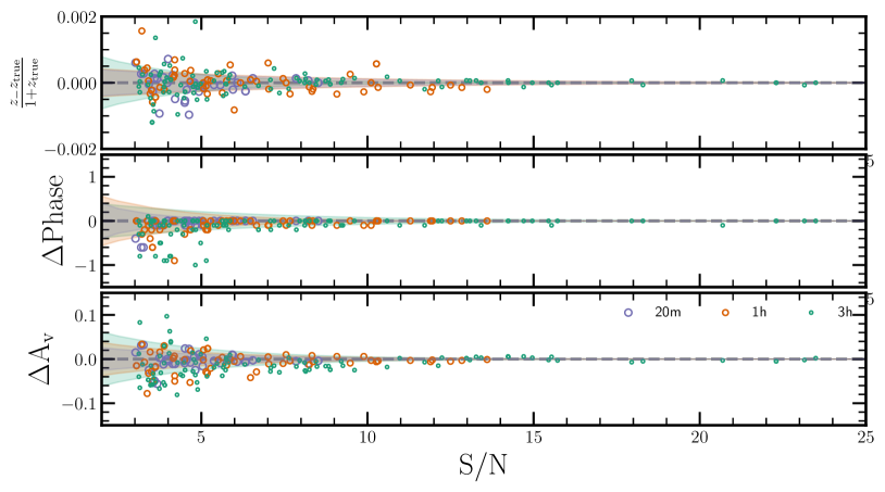
Figure 6 shows the dependence of the residuals of the recovered parameters on the S/N of the simulated spectrum for different exposure times. For clarity, this plot only shows those SNe from our simulation which do not contain any blending with host galaxy light. For redshift residuals (top row) from low to high S/N, three somewhat distinct S/N regimes can be observed — S/N , S/N , and S/N — which correspond to increasing accuracy of recovered parameters. Interestingly, while the redshift residuals and the dust-extinction residuals do not exhibit any appreciable bias in their measurements relative to S/N, the recovered phase shows a clear bias toward younger phases (at S/N ). We do not yet know the reason for this systematic phase bias. However, we note that a degeneracy between phase and redshift residuals has been observed by other studies (e.g., figure 14 in Blondin & Tonry, 2007). In this context, the recovered phases are underestimated for overestimated redshifts. The bias towards younger recovered phases at lower S/N is perhaps indicative of this degeneracy. While a larger range of simulated phases would allow for a full exploration of parameter space and correlations between the model parameters, given the limitations of the simulated models (we use a fiducial model for our SNe Ia with , see § 2.1), we delegate this to a future work.
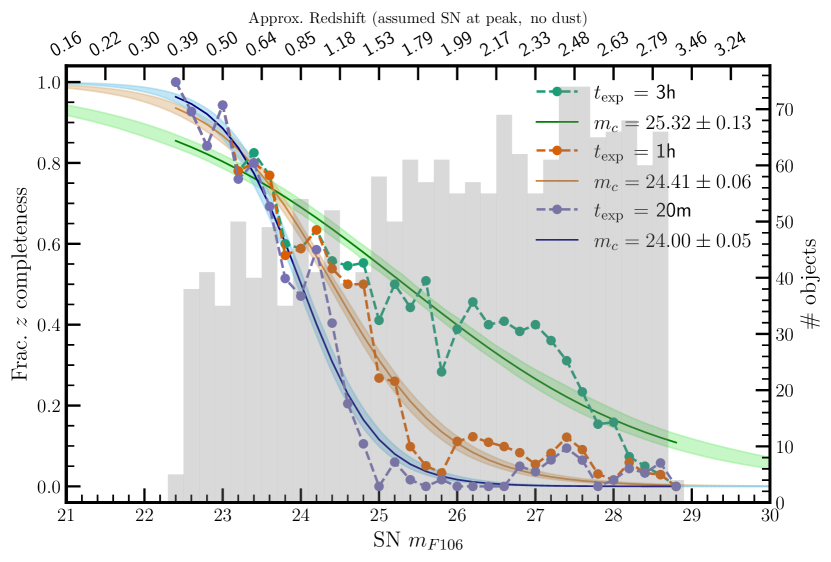
Figure 7 displays the efficiency of recovering redshifts as a function of SN Ia magnitude for our entire simulated sample of 1698 SNe Ia sources. Within each magnitude bin the figure shows the fraction of spectra that achieve a redshift accuracy of , measured through the absolute value of the redshift residuals . These redshifts are recovered solely from P127 spectroscopy of the SN Ia without any reliance on emission or absorption features in the host galaxy spectrum. While there is an implicit assumption here that the SN Ia classification efficiency from P127 spectra is 100% at all redshifts, this is a simplifying assumption we make given that any GO program on Roman will likely have classified a given transient as an SN Ia from photometric observations, prior to requesting prism spectroscopic observations. From preliminary work (done for HLTDS observations) we know that SN Ia classification efficiency is % for SNe Ia within , % within , and % for (Steven Rodney, private communication, using simulated P127 spectra of SNe Ia which are fit with SNID, Blondin & Tonry 2007). Therefore, while our completeness numbers here should be considered as upper limits, the ability to classify a P127 spectrum as belonging to an SN Ia only really impacts observations of SNe Ia at or SNe encountering extreme dust extinction.
The longest exposure time of 3 hr in our simulated observations achieves 50% efficiency for sources as faint as 25.5, and has much higher efficiency at brighter SN magnitudes and lower redshifts. Our shorter exposure times of 20 min and 1 hr achieve % completeness for SNe Ia brighter than 24 and 24.4 mag AB, respectively. Particularly for SNe Ia, this implies that the Roman P127 is quick and efficient at yielding high-S/N spectra and accurate redshifts. Note the gradual flattening of the curves as the exposure time is increased owing to increased numbers of fainter SN spectra being fit successfully, while of course the spectra of the brightest SNe are always fit successfully. For the longest exposure time considered, the gradual transition from high to low completeness also means that the 50% completeness cutoff (denoted by in the figure legend) is not sharp and the completeness drops to % beyond 27.5 mag AB.
We expect a 3 hr exposure time to reliably achieve 50% redshift completeness for all SN Ia redshifts in the range . These SNe Ia are expected to contribute most within cosmological analyses toward improving the dark energy FoM (Albrecht et al., 2006). Cosmological analyses usually assume that redshift errors have negligible effect on the uncertainty budget in their analysis (e.g., Betoule et al., 2014; Scolnic et al., 2018). We show in this work that this assumption should remain valid with cosmological analyses done using SN Ia redshifts inferred from Roman prism spectra. We find that the median redshift accuracy, median(), is on the order of a few tenths of a percent for any exposure time that provides S/N (Figure 6). How the uncertainty in redshift propagates to the dark energy FoM is part of a separate investigation (Macias et al., in prep.).
SNe Ia for which a host galaxy cannot be identified (e.g., Gupta et al., 2016), “hostless” SNe, are susceptible to being dropped from cosmological analyses which employ only host galaxy observations to estimate redshifts (e.g., Dark Energy Survey, Abbott et al. 2019; Pan-STARRS, Jones et al. 2018). Within the framework presented in this paper, i.e., SNe Ia without host galaxy blended light, we can recover accurate redshifts for Roman prism observations of hostless SNe (right column of Figure 5); therefore, allowing SNe Ia to be included in cosmological analyses which would otherwise be ignored.
While the primary goal of this work is not to optimize the ratio of P127 to imaging time for the HLTDS, we show a promising outlook for redshift inference from P127 spectra especially for SNe Ia at . Rose et al. (2021) presented several survey strategies with the ratio of prism to imaging time being one of the key unknown variables; the primary reference survey has 25% prism time amounting to 7.5 hr per visit split between a wide and a deep tier (900 s and 3600 s per object from the wide and deep tiers, respectively). Our 20 min and 1 hr exposure times are similar to the exposure time of a single HLTDS pointing, and achieve % completeness for SNe Ia brighter than 24 and 24.4 mag AB, respectively. However, if spectra from multiple visits are coadded, then the completeness will improve further. Figure 5 shows that the main problem hindering higher levels of redshift completeness is the blending of host galaxy and SN light causing confusion for fitting routines. In general for any rolling survey, disentangling the SN spectrum from the host galaxy spectrum will be somewhat easier given that the host galaxies will be repeatedly observed, allowing a subtraction of an uncontaminated host spectrum from a host+SN spectrum, as long as data are taken with a wide enough baseline such that SN light has faded.
4.1 Caveats
In this section, we discuss three caveats for the work presented here. Firstly, while the simulated spectra in the 2D dispersed images have the appropriate variable dispersion vs. wavelength for the Roman prism, the extracted 1D spectra do not yet have a variable dispersion. The 1D spectra have a constant wavelength sampling of 60 Å per pixel, corresponding to the approximately average dispersion for the Roman prism – allowing for the variable dispersion in the 1D spectra requires significant restructuring of the pyLINEAR code base and is a work in progress (note the process for 2D simulation and 1D extraction described in § 2.3 and § 3.1). As preliminary confirmation, we note that Figure 5 shows that the constant wavelength sampling for the 1D spectra does not hinder our ability to infer accurate redshifts, due to the broad absorption features in SN Ia spectra.
We also conduct an additional test to ensure that our constant sampling does not significantly affect our recovery of redshift. This is done by resampling the extracted 1D spectra to the expected dispersion of the P127 prism. The resampled spectra are then refit using the same pipeline as in § 3.2 and the newly recovered parameters are compared to the previous set of parameters recovered from the spectra with constant sampling. For the redshifts recovered with the resampled spectra, we observe improvements to a small subset of the sample – for objects within an additional 1–3% objects pass the redshift accuracy cut of . This translates to an improvement of mag in completeness for the 20 min and 1 hr exposure times and a mag improvement for the longest exposure time. However, we advise caution when interpreting these seemingly large improvements to the completeness depths since the resampling was done post the extraction of the 1D spectra. The sampling with the variable dispersion shows no significant changes at the highest redshifts but at lower redshifts shows an improvement in the efficiency of recovering redshifts. Therefore, the constant sampling provides a conservative estimate of Roman efficiency of redshift recovery for SNe Ia and should be employed for current survey planning purposes, whereas redshift recovery with the variable dispersion sampling deserves a more thorough investigation.
Secondly, because our goal is to evaluate redshift accuracies for SNe Ia from Roman P127 spectra, we do not include other classes of transients in our simulation (e.g., other Ia subtypes or core-collapse SNe), and lastly, we do not yet incorporate complex dust geometries in our simulation.
5 Summary
We have reported results from the analysis of 1698 simulated Roman P127 spectra of SN Ia with exposure times of 1200, 3600, and 10,800 s. The Roman P127 prism is exceptionally efficient at delivering high-S/N spectra, and therefore is particularly useful for inferring accurate redshifts based on absorption features in the continuum. We recover limiting magnitudes, i.e., 50% completeness, of 24.0, 24.4, and 25.3, for our three exposure times (although see preceding discussion about the steepness of completeness curves) under the requirement of . The procedure to employ pyLINEAR for simulating and extracting spectra, particularly for the case of the Roman P127 prism, is presented. The entire set of extracted 1D spectra, and simulated and recovered SN properties in tabular form, are available upon request.
References
- Abbott et al. (2019) Abbott, T. M. C., Allam, S., Andersen, P., et al. 2019, ApJ, 872, L30, doi: 10.3847/2041-8213/ab04fa
- Akeson et al. (2019) Akeson, R., Armus, L., Bachelet, E., et al. 2019, arXiv e-prints, arXiv:1902.05569. https://arxiv.org/abs/1902.05569
- Albrecht et al. (2006) Albrecht, A., Bernstein, G., Cahn, R., et al. 2006, arXiv e-prints, astro. https://arxiv.org/abs/astro-ph/0609591
- Bertin & Arnouts (1996) Bertin, E., & Arnouts, S. 1996, A&AS, 117, 393, doi: 10.1051/aas:1996164
- Betoule et al. (2014) Betoule, M., Kessler, R., Guy, J., et al. 2014, A&A, 568, A22, doi: 10.1051/0004-6361/201423413
- Blondin & Tonry (2007) Blondin, S., & Tonry, J. L. 2007, ApJ, 666, 1024, doi: 10.1086/520494
- Bruzual & Charlot (2003) Bruzual, G., & Charlot, S. 2003, MNRAS, 344, 1000, doi: 10.1046/j.1365-8711.2003.06897.x
- Calzetti et al. (2000) Calzetti, D., Armus, L., Bohlin, R. C., et al. 2000, ApJ, 533, 682, doi: 10.1086/308692
- Foreman-Mackey (2016) Foreman-Mackey, D. 2016, JOSS, 24, doi: 10.21105/joss.00024
- Foreman-Mackey et al. (2013) Foreman-Mackey, D., Hogg, D. W., Lang, D., & Goodman, J. 2013, PASP, 125, 306, doi: 10.1086/670067
- Foreman-Mackey et al. (2019) Foreman-Mackey, D., Farr, W., Sinha, M., et al. 2019, The Journal of Open Source Software, 4, 1864, doi: 10.21105/joss.01864
- Gupta et al. (2016) Gupta, R. R., Kuhlmann, S., Kovacs, E., et al. 2016, AJ, 152, 154, doi: 10.3847/0004-6256/152/6/154
- Guy et al. (2007) Guy, J., Astier, P., Baumont, S., et al. 2007, A&A, 466, 11, doi: 10.1051/0004-6361:20066930
- Harris et al. (2020) Harris, C. R., Millman, K. J., van der Walt, S. J., et al. 2020, Nature, 585, 357, doi: 10.1038/s41586-020-2649-2
- Holwerda et al. (2015) Holwerda, B. W., Keel, W. C., Kenworthy, M. A., & Mack, K. J. 2015, MNRAS, 451, 2390, doi: 10.1093/mnras/stv1125
- Hounsell et al. (2018) Hounsell, R., Scolnic, D., Foley, R. J., et al. 2018, ApJ, 867, 23, doi: 10.3847/1538-4357/aac08b
- Hunter (2007) Hunter, J. D. 2007, Computing in Science & Engineering, 9, 90, doi: 10.1109/MCSE.2007.55
- Jha et al. (1999) Jha, S., Garnavich, P. M., Kirshner, R. P., et al. 1999, ApJS, 125, 73, doi: 10.1086/313275
- Jones et al. (2018) Jones, D. O., Scolnic, D. M., Riess, A. G., et al. 2018, ApJ, 857, 51, doi: 10.3847/1538-4357/aab6b1
- Joye & Mandel (2003) Joye, W. A., & Mandel, E. 2003, in Astronomical Society of the Pacific Conference Series, Vol. 295, Astronomical Data Analysis Software and Systems XII, ed. H. E. Payne, R. I. Jedrzejewski, & R. N. Hook, 489
- Kümmel et al. (2009) Kümmel, M., Walsh, J. R., Pirzkal, N., Kuntschner, H., & Pasquali, A. 2009, PASP, 121, 59, doi: 10.1086/596715
- Kuntschner et al. (2010) Kuntschner, H., Bushouse, H., Kümmel, M., Walsh, J. R., & MacKenty, J. 2010, in Society of Photo-Optical Instrumentation Engineers (SPIE) Conference Series, Vol. 7731, Space Telescopes and Instrumentation 2010: Optical, Infrared, and Millimeter Wave, ed. J. Oschmann, Jacobus M., M. C. Clampin, & H. A. MacEwen, 77313A, doi: 10.1117/12.856421
- Mandel et al. (2014) Mandel, K. S., Foley, R. J., & Kirshner, R. P. 2014, ApJ, 797, 75, doi: 10.1088/0004-637X/797/2/75
- Oke & Gunn (1983) Oke, J. B., & Gunn, J. E. 1983, ApJ, 266, 713, doi: 10.1086/160817
- Paige & Saunders (1982) Paige, C. C., & Saunders, M. A. 1982, ACM Trans. Math. Software, 8, 43
- Pickles (1998) Pickles, A. J. 1998, PASP, 110, 863, doi: 10.1086/316197
- Pierel et al. (2018) Pierel, J. D. R., Rodney, S., Avelino, A., et al. 2018, PASP, 130, 114504, doi: 10.1088/1538-3873/aadb7a
- Pirzkal & Ryan (2017) Pirzkal, N., & Ryan, R. 2017, A more generalized coordinate transformation approach for grisms, Space Telescope WFC Instrument Science Report
- Pirzkal & Ryan (2020) —. 2020, The Dispersed infrared background in WFC3 G102 and G141 observations, Space Telescope WFC Instrument Science Report
- Pirzkal et al. (2016) Pirzkal, N., Ryan, R., & Brammer, G. 2016, Trace and Wavelength Calibrations of the WFC3 G102 and G141 IR Grisms, Instrument Science Report WFC3 2016-15, 25 pages
- Rose et al. (2021) Rose, B. M., Baltay, C., Hounsell, R., et al. 2021, arXiv e-prints, arXiv:2111.03081. https://arxiv.org/abs/2111.03081
- Ryan et al. (2018a) Ryan, R. E., J., Casertano, S., & Pirzkal, N. 2018a, PASP, 130, 034501, doi: 10.1088/1538-3873/aaa53e
- Ryan et al. (2018b) Ryan, R. E., Casertano, S., & Pirzkal, N. 2018b, Linear Reconstruction of Grism Spectroscopy I. Simulation and Extraction Examples, Space Telescope WFC Instrument Science Report
- Saunders et al. (2018) Saunders, C., Aldering, G., Antilogus, P., et al. 2018, ApJ, 869, 167, doi: 10.3847/1538-4357/aaec7e
- Scolnic et al. (2018) Scolnic, D. M., Jones, D. O., Rest, A., et al. 2018, ApJ, 859, 101, doi: 10.3847/1538-4357/aab9bb
- Spergel et al. (2015) Spergel, D., Gehrels, N., Baltay, C., et al. 2015, arXiv e-prints, arXiv:1503.03757. https://arxiv.org/abs/1503.03757
- Stoehr et al. (2008) Stoehr, F., White, R., Smith, M., et al. 2008, in Astronomical Society of the Pacific Conference Series, Vol. 394, Astronomical Data Analysis Software and Systems XVII, ed. R. W. Argyle, P. S. Bunclark, & J. R. Lewis, 505
- The Astropy Collaboration et al. (2018) The Astropy Collaboration, Price-Whelan, A. M., Sipőcz, B. M., et al. 2018, AJ, 156, 123, doi: 10.3847/1538-3881/aabc4f
- Virtanen et al. (2020) Virtanen, P., Gommers, R., Oliphant, T. E., et al. 2020, Nature Methods, 17, 261, doi: 10.1038/s41592-019-0686-2
- Wang et al. (2022) Wang, K. X., Scolnic, D., Troxel, M. A., et al. 2022, arXiv e-prints, arXiv:2204.13553. https://arxiv.org/abs/2204.13553
- Zhao et al. (2021) Zhao, X., Maeda, K., Wang, X., & Sai, H. 2021, MNRAS, 503, 4667, doi: 10.1093/mnras/staa3985
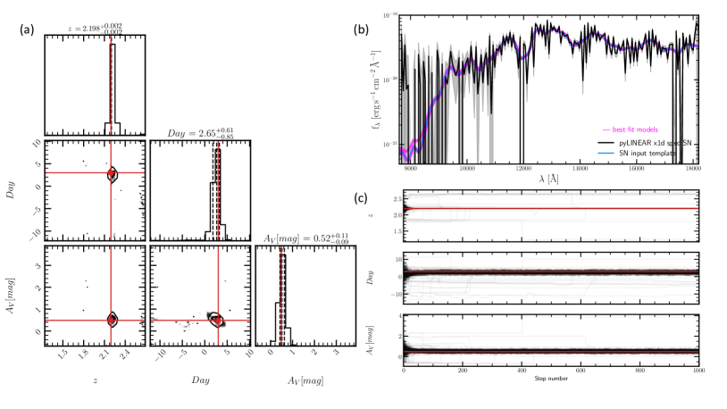
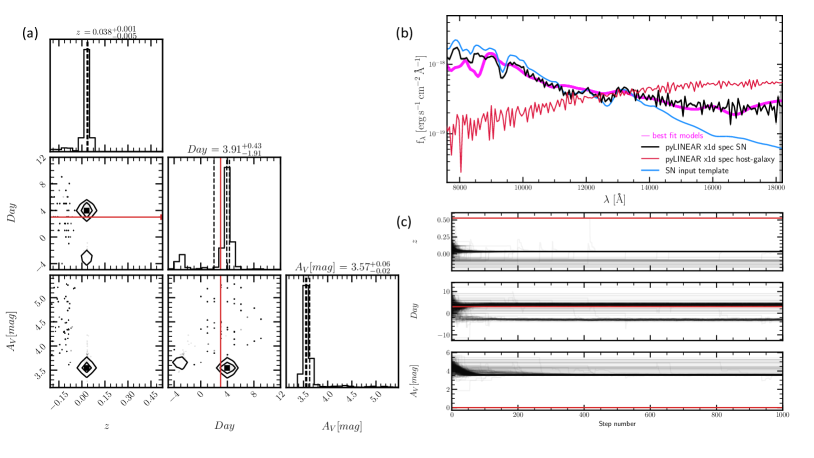
Appendix A Examples of Parameter Recovery
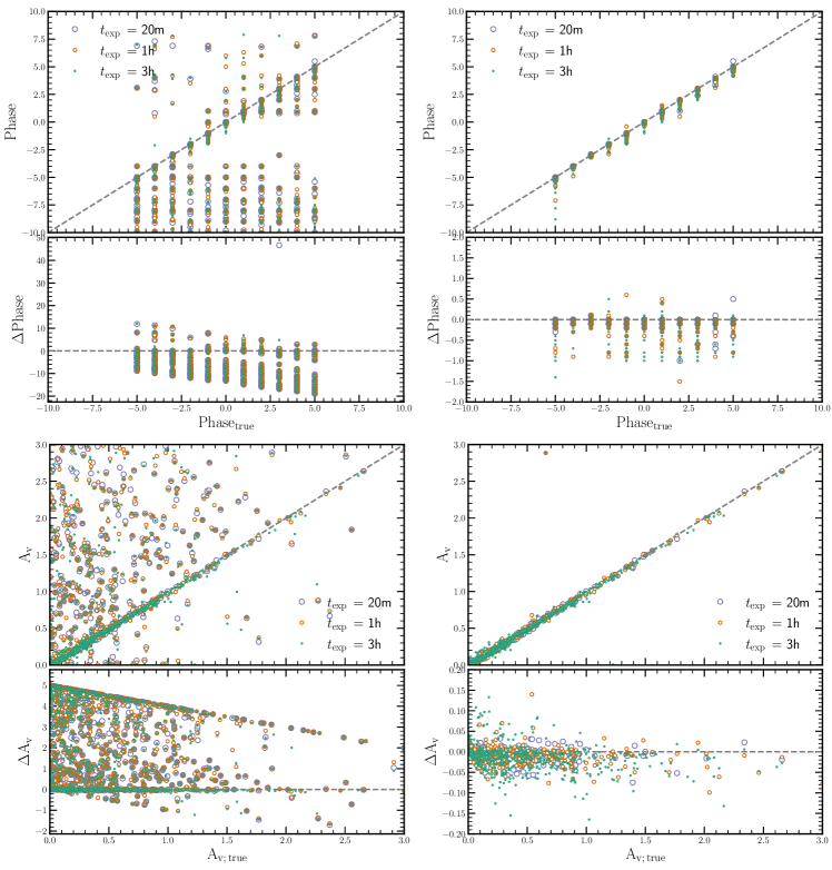
Figure 8 shows the recovery of phase and dust attenuation by our fitting pipeline. We also show two representative examples of parameter recovery by our fitting pipeline. Example 1 in Figure 9 shows the results of a successful fit, whereas example 2 in Figure 10 shows a common failure mode due to misidentification of absorption features within SNe Ia spectra that are caused by the red end continuum slope of the host galaxy (§ 3.2). Similar to the examples of blending shown in Figure 3 the fitting fails for the extracted spectrum in Figure 10 due to the being dominated by the addition of the host galaxy continuum slope, even though it is clear that the extracted spectrum has the SN absorption features at the correct wavelengths as seen in the input template.