Learning Mean Field Games: A Survey
Abstract
Non-cooperative and cooperative games with a very large number of players have many applications but remain generally intractable when the number of players increases. Introduced by Lasry and Lions, (2007) and Huang et al., (2006), Mean Field Games (MFGs) rely on a mean-field approximation to allow the number of players to grow to infinity. Traditional methods for solving these games generally rely on solving partial or stochastic differential equations with a full knowledge of the model. Recently, Reinforcement Learning (RL) has appeared promising to solve complex problems. By combining MFGs and RL, we hope to solve games at a very large scale both in terms of population size and environment complexity.
In this survey, we review the quickly growing recent literature on RL methods to learn Nash equilibria in MFGs. We first identify the most common settings (static, stationary, and evolutive). We then present a general framework for classical iterative methods (based on best-response computation or policy evaluation) to solve MFGs in an exact way. Building on these algorithms and the connection with Markov Decision Processes, we explain how RL can be used to learn MFG solutions in a model-free way. Last, we present numerical illustrations on a benchmark problem, and conclude with some perspectives.
1 Introduction
Since their introduction by Lasry and Lions (Lasry and Lions,, 2007) and Caines, Huang and Malhamé (Huang et al.,, 2006), mean field games (MFGs for short) have gained momentum as a powerful paradigm to study large populations of strategic agents. The main idea, borrowed from statistical physics, is to use the mean field distribution corresponding to the limiting mean field situation with an infinite number of players. All the individual interactions can then be replaced by the interaction between a representative player and the mean field distribution, which considerably simplifies the model and the analysis. This approximation relies on the assumption that the population is homogeneous and that the interactions are symmetric in the sense that each player interacts only with the empirical distribution of the other players. The solution to the MFG provides an -Nash equilibrium for the corresponding -player game, with going to as goes to infinity. Furthermore, under suitable assumptions, -player Nash equilibria or social optima converge to the corresponding mean field equilibrium or social optimum. Such results build on the idea of propagation of chaos (Sznitman,, 1991) but are more subtle since the players are not simple particles but rational agents making optimal decisions and reacting to other players’ decisions (Lacker,, 2017; Cecchin and Pelino,, 2019; Lacker,, 2020; Cardaliaguet et al.,, 2019).
1.1 Mean field games
General intuition.
We start this survey by defining at a high level what a Mean Field Game (MFG) is. Intuitively, a Mean Field Game is a game with an infinite number of identical players. All players have a similar behavior, i.e. they are symmetric: we do not need to retain the identity of a player as part of its state. Furthermore, as we have an infinite number of players, we can replace the atomic players by their distributions over the state (and sometimes action) space. The population’s distribution enables to focus only on the interaction between a so-called representative player, which is sampled from the population’s distribution, and the population’s distribution itself. Our ultimate goal is to compute a Nash equilibrium, which corresponds to the situation where no player has an interest in deviating from its current behavior, provided that the other players do not deviate either. Looking for a Nash equilibrium makes the assumption that the players are all perfectly rational, i.e their goal is to maximize their own reward (or minimize their cost).
Most of the literature focuses on two types of problems: Nash equilibria or social optimum. These two settings are typically referred to respectively as mean field game and mean field control (or control of McKean-Vlasov dynamics), (Bensoussan et al.,, 2013; Carmona and Delarue, 2018a, ). In both cases, the solutions are typically characterized through optimality conditions taking the form of a coupled system of forward-backward equations. The forward equation describes the evolution of the population distribution while the backward equation represents the evolution of the value function (i.e. the utility of its behaviour) for a representative player. In the continuous time and continuous space setting, the equations can be partial differential equations (PDEs) (Lasry and Lions,, 2007) or stochastic differential equations (SDEs) of McKean-Vlasov type (Carmona and Delarue,, 2013) depending on whether one relies on the analytical approach or the probabilistic approach. We refer to e.g. Bensoussan et al., (2013); Carmona and Delarue, 2018a ; Carmona and Delarue, 2018b ; Achdou et al., (2020) for more details. In this survey, we will focus on the discrete time case, which is closer to the framework of Markov Decision Processes (Bertsekas and Shreve,, 1996; Puterman,, 2014).
Example.
As a typical example, we can consider crowd motion. Each player is an agent represented by her position and is able to control her velocity so as to reach a target destination while minimizing the effort made to move. Typically, passing through a crowded region, i.e. a region with a high density of players, requires extra efforts or reduces the velocity, which creates some congestion. If we assume that the number of agents is extremely large and that these agents are homogeneous and have symmetric interactions, then we can approximate the empirical distribution of positions by the mean field distribution corresponding to the limiting regime with an infinite population. This allows to simplify tremendously the computation of a Nash equilibrium because we only need to compute the optimal policy of the representative player.
Remark 1 (On MFGs and non-atomic anonymous games).
Games modeling infinite populations of agents have also been studied in the framework of non-atomic anonymous games, which have founds applications particularly in economics, see e.g. Aumann, (1964); Schmeidler, (1973); Aumann and Shapley, (2015). In such games, there is typically a continuum of players, indexed by, say, real numbers in and the population is represented by a non-atomic measure on . Each player perceives the other players through some aggregate quantity. Although this is very similar to the MFG framework, the key difference is that the MFG approach completely avoids representing the continuum of players. The main idea is to exploit the homogeneity of the population and the symmetry of interactions to simplify the characterization of an equilibrium: it is sufficient to understand the behavior of a single representative player facing a distribution representing the aggregate information available to this player. The analysis is greatly simplified, particularly when it comes to stochastic games. Defining rigorously a continuum of random variables with nice measurability properties is not trivial, as noticed for instance by Duffie and Sun, (2012); Sun, (2006) who used the concept of rich Fubini extension to develop an exact law of large numbers. The MFG framework allows to carry out the mathematical analysis of Nash equilibria without requiring such sophistication.
Some applications.
MFGs have found various applications such as population dynamics (Guéant et al.,, 2011; Achdou et al., 2017a, ; Cardaliaguet et al.,, 2016), crowd motion modeling (Achdou and Lasry,, 2019; Burger et al.,, 2013; Djehiche et al., 2017a, ; Aurell and Djehiche,, 2019; Achdou and Laurière,, 2016; Chevalier et al.,, 2015), flocking (Nourian et al.,, 2010, 2011; Grover et al.,, 2018; Perrin et al., 2021b, ), opinion dynamics and consensus formation (Stella et al.,, 2013; Bauso et al., 2016a, ; Parise et al.,, 2015), autonomous vehicles (Huang et al.,, 2017; Shiri et al.,, 2019), epidemics control (Laguzet and Turinici,, 2015; Hubert and Turinici,, 2018; Elie et al., 2020a, ; Lee et al., 2021b, ; Aurell et al.,, 2022; Doncel et al.,, 2022), macro-economic models (Achdou et al., 2017b, ; Elie et al., 2019b, ; Achdou et al., 2017b, ; Achdou et al.,, 2014; Chan and Sircar,, 2015; Gomes et al., 2014a, ; Djehiche et al., 2017b, ), finance (Lachapelle et al.,, 2016; Cardaliaguet and Lehalle,, 2018; Lasry and Lions,, 2007; Lachapelle et al.,, 2016; Gomes and Saúde,, 2020; Carmona,, 2020), energy production and management (Alasseur et al.,, 2020; Couillet et al.,, 2012; Elie et al., 2019a, ; Bagagiolo and Bauso,, 2014; Kizilkale et al.,, 2019; Li et al.,, 2016; Guéant et al.,, 2011; Achdou et al.,, 2016; Chan and Sircar,, 2017; Graber and Bensoussan,, 2018), security and communication (Mériaux et al.,, 2012; Samarakoon et al.,, 2015; Hamidouche et al.,, 2016; Yang et al.,, 2017; Kolokoltsov and Bensoussan,, 2016; Kolokoltsov and Malafeyev,, 2018), traffic modeling (Bauso et al., 2016b, ; Salhab et al.,, 2018; Huang et al.,, 2019; Tanaka et al.,, 2020; Cabannes et al.,, 2021) or engineering (Djehiche et al., 2017b, ).
Numerical methods.
Most existing numerical methods for MFGs and MFC problems are based on the aforementioned optimality conditions phrased in terms of PDEs or SDEs. Such approaches typically rely suitable discretizations, e.g. by finite differences (Achdou and Capuzzo-Dolcetta,, 2010; Achdou et al.,, 2012; Briceño Arias et al.,, 2018, 2019), semi-Lagrangian schemes (Carlini and Silva,, 2014, 2015), or probabilistic approaches (Chassagneux et al.,, 2019; Angiuli et al.,, 2019). We refer to e.g. Achdou and Laurière, (2020); Lauriere, (2021) for recent surveys on these methods. Although these methods are very well understood and very successful in small dimension, they cannot tackle MFGs with high dimensional states or controls due to the curse of dimensionality (Bellman,, 1957). To address this limitation, stochastic methods based on approximations by neural networks have recently been introduced by Carmona and Laurière, (2021, 2019); Fouque and Zhang, (2020); Germain et al., (2022) using optimality conditions for general mean field games, by Ruthotto et al., (2020) for MFGs which can be written as a control problem, and by Cao et al., (2020); Lin et al., (2020) for variational MFGs in connection with generative adversarial networks (GANs) (Goodfellow et al.,, 2014). We refer to Hu and Laurière, (2022) for a recent survey on machine learning methods for control and games, with applications to MFGs and MFC problems. However, these methods still try to solve the problems in an exact way by relying on exact computations of gradients by exploiting the full knowledge of the model. The learning methods we focus on in this survey aim at solving MFGs and MFC in a model-free fashion to foster the scalability of numerical methods for these problems.
1.2 Learning
Two notions of learning.
The second question we need to answer before diving more into the survey is what learning means in our context. There are mainly two interpretations of learning. The first one comes from game theory and economics and, according to Fudenberg et al., (1998), refers to “The theory of learning in games […] examines how, which, and what kind of equilibrium might arise as a consequence of along-run non equilibrium process of learning, adaptation, and/or imitation.” From this point of view, the main focus is on how the players iteratively adjust their behavior until convergence to an equilibrium. The second interpretation of learning is mainly used in Machine Learning and in Reinforcement Learning. As Mitchell et al., (1997) puts it, "a computer program is said to learn from experience E with respect to some class of tasks T and performance measure P if its performance at tasks in T, as measured by P, improves with experience E.” In this concept, the concept of learning is very related to the idea of improving one’s performance by using data or samples. In this survey, we are interested in delineating these two notions of learning while explaining how they can be combined.
Learning in games.
More specifically, we will focus on learning in MFGs. This research direction finds its roots in the literature on learning in games, which goes back to the works of Shannon, (1959) and Samuel, (1959). Since then, a lot of progress has been made but remains mostly limited to games with a small number of players. Many of the recent breakthrough results have been obtained using a combination of reinforcement learning (Sutton and Barto,, 2018) and deep neural networks (Goodfellow et al.,, 2016), see e.g. Go (Silver et al.,, 2016, 2017, 2018), Chess (Campbell et al.,, 2002), Checkers (Schaeffer et al.,, 2007; Samuel,, 1959), Hex (Anthony et al.,, 2017), Starcraft II (Vinyals et al.,, 2019), poker games (Brown and Sandholm,, 2017, 2019; Moravčík et al.,, 2017; Bowling et al.,, 2015) or Stratego (McAleer et al.,, 2020).
Learning in mean field games.
The goal of this survey is to review the quickly growing literature at the intersection of learning and MFGs. We hope that combining mean field approximations, which allow to tackle large population games, and reinforcement leanring, which allows to handle highly complex environments, we will be able to solve multi-agent systems at a very large scale, both in terms of population size and model complexity.
1.3 Outline of the survey
In the rest of this section, we introduce a few useful notation. In Section 2, we present several settings of MFG and MFC problems that have appeared in the literature. We stress the similarities and the differences, in terms of definitions and in terms of solutions. In Section 3, we present algorithms to compute MFG and MFC solutions. We start by recalling some classical methods to solve MDPs and then describe mainly two classes of algorithms to find Nash equilibria in MFGs. These algorithms are based on iteratively updating the mean field and the policy, so we refer to them as iterative methods. Building on these methods and the connection between MDPs and RL, we explain in Section 4 how RL and deep RL methods can be adapted to solve MFGs and MFC problems. Section 5 discusses metrics that can be used to assess the numerical convergence of algorithms and illustrate some of the methods on a representative MFG example. Finally, we conclude in Section 6 with a short summary and some perspectives.
1.4 Useful notation
Here we introduce some general notation that we use throughout the text:
-
•
and denote a finite state set and a finite action set respectively.
-
•
denotes the cardinal of a set .
-
•
denotes the set of subsets of a set .
-
•
is the set of probability distributions on a set ; when is finite (which is generally the case for us), it is also identified with the corresponding simplex in the Euclidean space of dimension , and we view probability distributions as (normalized) vectors in .
-
•
is understood as the set of all maximizers.
-
•
denote respectively probability and expectation.
-
•
Unless otherwise specified, bold symbols denote time-dependent objects, which can be viewed as functions of time or as sequences indexed by time steps.
-
•
We will use subscripts with for time indices and superscript with for iteration indices in algorithms.
-
•
Given a probability distribution on a set and a function , .
2 Definition of the problems
In this section, we present several settings of MFGs which depend on how time is involved (or not) in the problem. These settings correspond to different applications and different notions of Nash equilibrium. Here, we focus on four settings, that can be summarized as follows. We start with games in which the agents take a single decision. There is no notion of time intrinsic to the game so we call them static MFGs. We then turn to games in which there is a dynamical aspect. In such games, each agent has a state that evolves along time, and she can act on this evolution. At the level of the population, in some situations, we can expect the distribution of states to converge to a stationary regime, in which the population is stable at a macroscopic level, even though each agent’s state is possibly changing. We refer to this setting as a stationary MFG. In other cases, one wants to understand not only the stationary regime, but how the population evolves, starting from an initial configuration. This is relevant for applications in which the agents’ behaviors change along time, for instance because there is a finite horizon at which the game stops. We call such games evolutive MFGs. This setting comes at the expense of having policies and mean-field terms that depend on time and are thus harder to compute. To mitigate this complexity while not falling completely into the stationary regime, an intermediate model has been introduced. The idea is to try to keep the best of the stationary and evolutive settings by considering a proxy for the whole evolution of the distribution. We call this setting discounted stationary MFGs. In the rest of this section, we define each setting as well as the corresponding notion of Nash equilibrium, along with relevant concepts.
2.1 Static MFG
Let be a finite action space. The behavior of one player, called a strategy, is an element of , that is a distribution over the action set. In this setting, the behavior of the population is also an element of . We denote a generic element of by , and we denote a generic individual behavior and a generic population behavior by and respectively.
Besides the action space , the model is completely defined by a reward function . Given a population behavior , the reward of a player using is defined as the expected reward when sampling an action according to :
The reward function can typically encode crowd aversion or attraction towards a population action of interest.
Example 1.
One of the first examples in the MFG literature is the problem of choosing a starting time for a meeting, introduced and solved explicitly by Guéant et al., (2011). In this problem, the players choose at what time they want to arrive to the meeting room so that they are neither too late nor too early. The global outcome is the time at which the meeting actually starts, which is not known in advance and depends on the everyone’s arrival time. Despite its name, there is no dynamic aspect in the original formulation of the example. Another popular example is the problem in which each agent chooses a location on a beach, see e.g. Perrin et al., (2020). They want to put their towel close to an ice cream stall but not in a very crowded area. The global outcome is the distribution of towels on the beach. To be specific, a simple model can be as follows: , which represents possible positions on the beach, is the position of the stall, and the reward is , where the first term penalizes the distance to the stall and the second term penalizes choosing a location at which the density of people is high.
A central concept is the notion of best response. Let us define the (set-valued) best response map by:
Definition 1 (Static MF Nash Equilibrium).
is a static mean field Nash equilibrium (static MFNE) if it satisfies the following condition:
The above definition has the advantage to clearly show that the equilibrium is a fixed point of .
Another point of view, which will be useful in the dynamic settings presented in the sequel, consists in saying that the equilibrium is given by a pair of a representative agent’s behavior and the population’s behavior. Here, it means that the equilibrium is a pair such that:
-
1.
is optimal for the representative agent facing , i.e., ,
-
2.
corresponds to the population behavior when all every agent uses , i.e., .
The second point represents the fact that all the agents are “rational in the same way” and hence, at equilibrium, adopt the same behavior. This viewpoint is unnecessarily complicated in this setting as alone is enough to define the MFNE, but will be useful in dynamic settings.
Remark 2.
Consistently with the literature on normal-form games (Fudenberg and Tirole,, 1991), each player chooses a distribution over actions without seeing the strategy chosen by other players and the resulting distribution at the population level. Each agent thus tries to anticipate, in a rational way, the distribution generated by other players’ actions.
A Nash equilibrium corresponds to a situation in which no selfish player has any incentive to deviate unilaterally. However, it is not necessarily a situation that is optimal from the point of view of the whole population. The notion of social optimum is discussed below in Section 2.7.
Remark 3.
Although we provided an intuitive explanation for in terms of a continuum of players, we want to stress that in the definition of an MFG equilibrium or social optimum, we actually never need to consider a continuum of players. As already pointed out in Remark 1, this shortcut is one of the main advantages of the MFG paradigm compared with non-atomic anonymous games.
2.2 Notations for the dynamic setting
In contrast with the static case, in the dynamic setting, each agent has a state which evolves in time. The agent can influence the evolution of their own state using actions. The population’s state is the distribution of the agents’ states, the joint distribution of their states and actions. This is what constitutes the mean field, with which every agent interacts through its dynamics and its rewards.
As far as the population distribution is concerned, we will consider mainly two types of settings: one in which the population distribution is fixed, and one in which it can also evolve. Typically, the former is conceptually simpler and easier to compute but the latter is more realistic since many real world applications involve a population evolving in time. In each cases, several variants can be considered. For the sake of brevity, we shall focus only on the main ideas.
We will consider discrete time models, with time typically denoted by . If a time horizon is imposed, we will typically use the notation . Let be a finite state space. A stationary policy is an element of . In this setting, we assume that the interactions occur through an aggregate variable which represents the behavior of the population. A mean field state is an element of , which is the set of probability distributions on the state space. It represents the state of the population at a given time. We denote generic elements of , , and respectively by , , , and .
Depending on the setting, we might consider policies that depend on time or on an initial distribution. More details will be provided below, as we introduce several setups.
Remark 4.
To alleviate the presentation, we choose to focus on finite state and action spaces and discrete time. In some cases, continuous space or continuous time models might be more relevant. They are typically analyzed using partial differential equations or stochastic differential equations. Suitable discretizations can lead to (possibly non-trivial) approximations of these models with discrete ones, as presented in this survey, see e.g. Hadikhanloo and Silva, (2019) for more details on the convergence of a finite MFG to a continuous one. We do not discuss in detail the continuous settings here and we refer the interested reader to the literature, e.g., Huang et al., (2006); Lasry and Lions, (2007); Bensoussan et al., (2013); Carmona and Delarue, 2018a ; Carmona and Delarue, 2018b .
2.3 Background on MDPs
We recall a few important concepts pertaining to optimal control in discrete time for a single agent. We will only review the main ideas and we refer to e.g. Bertsekas and Shreve, (1996); Puterman, (2014) for more details. The notion of Markov decision processes will play a key role in the description of dynamic MFGs.
2.3.1 Stationary MDP
A stationary Markov decision process (MDP) is a tuple where is a state space, is an action space, is a transition kernel, is a reward function and is a discount factor. Using action when the current state is leads to a new state distributed according to and produces a reward . The reward could be stochastic but to simplify the presentation, we consider that is a deterministic function of the state and the action. A stationary policy , provides a distribution over actions for each state. The goal of the MDP is to find a policy which maximizes the total return defined as the expected (discounted) sum of future rewards:
subject to:
where is an initial distribution whose choice does not influence the set of optimal policies.
Assuming the model is fully known to the agent, the problem can be solved using for instance dynamic programming. The state-action value function associated to a stationary policy is defined as:
| (1) |
By dynamic programming, it satisfies the following fixed point equation with unknown :
where denotes the Bellman operator associated to :
| (2) |
We recall that the expectation is to be understood as:
| (3) |
The optimal state-action value function is defined as:
| (4) |
It satisfies the fixed point equation:
| (5) |
where denotes the optimal Bellman operator:
| (6) |
with
| (7) |
It is also convenient to introduce the (state only) value function associated to a policy and the (state only) optimal value function , where is an optimal policy. These value functions can also be characterized as fixed points of two Bellman operators. Note that these objects are all independent of time, as we search for a stationary solution.
2.3.2 Finite Horizon MDP
One can also consider problems set with a finite time horizon. A finite-horizon Markov decision process (MDP) is a tuple where is a state space, is an action space, is a time horizon, is a transition kernel, and is a reward function. At time , using action when the current state is leads to a new state distributed according to and produces a reward . A policy , provides a distribution over actions for each state at time . The goal of the MDP is to find a policy which maximizes the total return defined as the expected (discounted) sum of future rewards:
subject to:
where is an initial distribution whose choice does not influence the set of optimal policies.
Here again, assuming the model is known to the agent, the problem can be solved using for instance dynamic programming. The state-action value function associated to a stationary policy is defined as:
The optimal state-action value function is defined as:
| (8) |
Here again, we can introduce the (state only) value function associated to a policy: , and the optimal value function: , is an optimal policy.
Formally, the finite-horizon MDP can be restated as a stationary MDP by incorporating the time in the state. However, it can be simpler to directly tackle this MDP using techniques that are specific to the finite-horizon setting. In particular we stress that, in contrast with the stationary setting presented above, the value functions are here characterized by equations which are not fixed point equations but backward equations. They can be solved by backward induction, as we will discuss in the sequel (see Section 3). For more details on finite-horizon MDP we refer to e.g. (Puterman,, 2014).
2.4 Stationary setting
Here we consider an infinite horizon model, meaning that there is no terminal time. We assume that the players interact through a stationary distribution, which represents a steady state of the population. The model is defined by a tuple consisting of:
-
•
a state space and an action space ,
-
•
a one-step transition probability kernel ,
-
•
a one-step reward function ,
-
•
and a discount factor .
The main difference with standard MDPs as recalled in Section 2.3 is the presence of a third input for and , which is an element of the mean field state space . It plays the role of the population’s state, which influences the dynamics and the rewards.
Assume the state of the population is given by and consider a representative agent using policy . The total, discounted reward of this player is given by:
| (9) |
where the state of the agent evolves according to:
| (10) |
Remark 5 (State-action distribution).
An extension of the above model is to consider that the agents interact through the state-action distribution. In this case, assume the state of the population is given by and consider a representative agent using policy . The total, discounted reward of a representative player is given by:
where the state of the agent evolves according to:
with denoting the first marginal of . This setting is considered for instance by Guo et al., (2019); Guo et al., 2020a . MFG with interactions through state-action distributions have first been studied by Gomes et al., 2014b ; Gomes and Voskanyan, (2016) and are sometimes referred to as extended MFGs or MFG of controls, see Cardaliaguet and Lehalle, (2018); Kobeissi, (2022). Let us stress that a state-action distribution is not always a product distribution, meaning that for some there is no and such that . In fact, in general the actions of a player are given by a function of the player’s states, and hence the joint distribution cannot be written as a product. To simplify the presentation, we restrict our attention to interactions through state-only distributions but most of the ideas can be extended to state-action distributions. The interested reader is referred to Carmona and Delarue, 2018a (, Section 4.6) and the references therein.
This stationary MFG setting has been studied for instance by Subramanian and Mahajan, (2019) with applications to malware spread and investments in product quality, by Guo et al., (2019); Guo et al., 2020a with applications to auctions and by Angiuli et al., 2022b in the context of linear-quadratic MFGs.
Example 2 (Repeated auction game).
As an example, Guo et al., (2019) consider a repeated game in which the players bid in an auction game. At a given time, a player’s state and action are respectively her budget and her bid for the next auction.
The evolution of the population is given by a transition matrix defined by: for all and ,
| (11) |
In words, is the next state distribution for a representative agent starting with state distribution and using policy while the population has state distribution .
Given a population state, the goal for a representative agent, is to find the best reaction, i.e., a policy that maximizes their total reward. We define the (set-valued) best response map by:
and the (set-valued) population behavior map by:
| (12) |
which is the stationary distribution obtained when using (that we assume to be unique).
Remark 6.
Note that solving the equation is not trivial since is involved in the transition matrix . We come back to this point in Section 3.3.1.
Definition 2 (Stationary MF Nash Equilibrium).
A pair is a stationary mean field Nash equilibrium (stationary MFNE) if it satisfies the following two conditions:
-
•
;
-
•
.
Alternatively, an equilibrium can be defined as a fixed point: is a stationary MFNE policy if it is a fixed point of , and is a stationary MFNE distribution if it is the stationary distribution of a stationary MFNE policy.
In this setting, the state-action value function associated to a stationary policy for a given distribution is defined as:
The problem then reduces to a standard stationary MDP, parameterized by . By dynamic programming, satisfies the fixed point equation:
| (13) |
where denotes the Bellman operator associated to and :
| (14) |
where
| (15) |
The optimal state-action value function is defined as:
It satisfies the fixed point equation:
| (16) |
where denotes the optimal Bellman operator associated to :
| (17) |
with
| (18) |
Note that the functions and , and the operators and are all independent of time, as we search for stationary equilibria.
2.5 Evolutive setting
We next turn our attention to a model in which not only the agents’ state can evolve, but the population’s distribution too. In this case, the mean field is not stationary. At each time step, the transition and the reward of every agent depends on the current distribution instead of the stationary one. The model is defined by a tuple consisting of:
-
•
a state space and an action space ,
-
•
an initial distribution ,
-
•
a time horizon ,
-
•
a sequence of one-step transition probability kernels , ,
-
•
a sequence of one-step reward functions , .
In this context, a population behavior is a mean field flow, generally denoted by , which is an element of . A policy is an element of , generally denoted by . We use bold letter to stress that these are sequences, which can also be viewed as functions of time.
The total reward is:
subject to the following evolution of the agent’s state:
| (19) |
This evolution is analogous to (10) except that the stationary mean-field state is replaced by the current mean-field state at time .
We assume that the transition and the reward are such that the total reward is well defined.
Remark 7 (Finite and infinite horizon discounted settings).
Our notation covers two very common settings:
-
•
Finite horizon: .
-
•
Infinite horizon: . In this case, it is common to assume that is independent of time, and that is of the form where is independent of time and bounded.
Note that even in the infinite horizon setting and even if and are stationary (constant with respect to the time parameter ), in general the optimal policy still depends on time. This is in contrast with the stationary setting (section 2.4) and is due to the fact that the population distribution starts from and evolves. The player needs to take that into account in its decisions. To be specific, even if is independent of time, the reward associated to a fixed state-action pair is at time and at time . Unless the mean-field state is stationary, in general the two reward values will be different.
Example 3 (Crowd motion).
This setting is probably the most commonly studied one in the MFG literature. As a typical example, we can think of a model for crowd motion in the spirit of e.g. Achdou and Lasry, (2019): the agents start from an initial position and want to reach a point of interest while avoiding crowded areas. Because the population distribution changes as the agents move, looking for a stationary solution is not satisfactory if we want to compute the evolution of the whole population. This is because a stationary solution would only give the optimal policy (from the Nash equilibrium perspective) against the stationary distribution, and would not be able to recover the full evolution of the agents. In contrast, a time-dependent policy in the evolutive setup is able to adjust the agents’ behavior step by step.
Remark 8.
Discrete time finite state mean field games have been introduced by Gomes et al., (2010). In the model analyzed therein, the players can directly control their transition probabilities. Note that the model we consider here is a bit more general since the transition probabilities are functions of the actions, but they are not necessarily chosen freely by the players.
We define the (set-valued) best response map by:
Let us define the population behavior map by:
| (20) |
where this flow is defined by:
| (21) |
When the context is clear, we will simply write .
Definition 3 (Evolutive MFG Nash Equilibrium).
A pair is an evolutive mean field Nash equilibrium (evolutive MFNE) if it satisfies the following two conditions:
-
•
Best response: ;
-
•
Mean field flow: .
Alternatively, an evolutive MFNE can be defined as a fixed point: is an evolutive MFNE policy if it is a fixed point of , and is an evolutive MFNE flow if it is the mean field flow generated by an evolutive MFNE policy.
The state-action value function associated to a policy and the optimal state-action value function are defined analogously to standard MDP but parameterized by . We denote them respectively by and .
For the sake of completeness, let us provide more details in the finite horizon setting. Assume . The state-action value function associated to a policy for a given distribution is defined as:
The optimal state-action value function is defined as:
2.6 Discounted stationary setting
We now discuss a setting that is somehow between the stationary and the evolutive ones. Note that in the stationary setting, we focus on the stationary distribution of the population while in the evolutive setting, we care about the entire sequence starting from . In the first case, we can restrict our attention to stationary policies, whereas this is not possible in the second case, as highlighted in Remark 7. An intermediate approach consists in replacing the distribution at time by an aggregate which keeps some memory of , instead of the stationary distribution.
The model is defined by a tuple consisting of:
-
•
a state space and an action space ,
-
•
an initial distribution ,
-
•
a one-step transition probability kernel ,
-
•
a one-step reward function ,,
-
•
a discount factor .
We define the discounted distribution as:
where follows the dynamics (21) but with for all after starting from at time , and with the mean-field term replaced by , i.e.,
This formulation allows us to work with a single distribution, which plays the role of a summary of what happens along the mean field flow. In contrast with the stationary MFG setting, here the initial distribution still influences the mean field term, namely, . However, we can restrict our attention to stationary policies just as in the stationary MFG setting.
Example 4 (Exploration).
In (Perrin et al.,, 2020; Geist et al.,, 2021), this setting has been used for an MFG in which the agents explore the spatial domain. From the point of view of the population, it amounts to maximizing the entropy of the distribution. The discounted stationary distribution can be used as a proxy to evaluate with a single distribution how well the population explore the state space.
Remark 9.
The discounted distribution can be interpreted as the stationary distribution of an agent who starts with distribution , uses policy but has a probability to stop at any time step. To be specific, let be a random variable with geometric distribution on with parameter . Let us denote by is the distribution of , where:
Then we have: for every ,
When , , so we obtain that:
Definition 4 (Discounted stationary MFG Nash Equilibrium).
A pair is a discounted stationary mean field Nash equilibrium (discounted stationary MFNE) if it satisfies the following two conditions:
-
•
;
-
•
.
Alternatively, is a discounted stationary mean field Nash equilibrium distribution if it is a fixed point of: .
2.7 Social optimum and Mean Field Control
The notions of MFNE discussed above correspond to non-cooperative games, in which each player maximizes her own reward while trying to anticipate the behavior of other selfish agents. A different question consists in considering that the agents are cooperative and try to maximizer a social welfare criterion by choosing together a suitable policy. This situation can also be interpreted as an optimization problem from the point of view of a social planner, who tries to figure out which behavior is optimal from the society standpoint.
Static setting.
The social welfare function is defined as the reward obtained on average by the agents:
A strategy is a static mean field social optimum (static MFSO) if it maximizes the social welfare function .
Stationary case.
The total, discounted social welfare associated to a policy is:
subject to:
where is the stationary distribution induced by . Here we see that perturbing changes , which is reflected in the third argument of the transition function and the reward function. An optimal stationary policy is a maximizing . This setting has been considered by Subramanian and Mahajan, (2019) or by Angiuli et al., 2022b .
Evolutive case.
The total social welfare is:
subject to the following evolution of the agent’s state:
An optimal policy is a maximizing .
Discounted stationary case.
The total social welfare is:
subject to:
where is the discounted distribution introduced in Section 2.6.
Price of anarchy.
The average reward obtained by a representative player can only be higher in an MFSO than in an MFNE, by the very definition of a social optimum. The discrepancy between the two situations is quantified by the following notion the price of anarchy (PoA). In the static setting, it is defined as:
In the denominator, denotes the set of static MFNE. The PoA can be defined analogously in the other settings.
The term “Price of Anarchy” has been coined by Koutsoupias and Papadimitriou, (1999). Since then, this notion has been widely studied in game theory and can be viewed as a way to measure the inefficiency of Nash equilibria (Roughgarden and Tardos,, 2007). In the context of MFGs, it has been studied e.g. by Lacker and Ramanan, (2019) in a static setting, and by Carmona et al., 2019a in a dynamic setting.
2.8 Extensions
We conclude this section by mentioning a few extensions. For the sake of readability, we use the basic settings described above in the sequel. However, several variants have been considered in the literature.
Multiple populations.
Mean field theory allows us to approximate a homogeneous population of individuals by the limiting probability distribution. In multi-population MFGs, there is a finite number of sub-populations, each of them representing a homogeneous group of agents. The transition function and the reward function are the same for all the agents of one sub-population, but may be different from one group to the other. In this way, the MFG paradigm can still be used. We refer for instance to Huang et al., (2006); Feleqi, (2013); Cirant, (2015); Bensoussan et al., (2018) for an analytical approach and to Carmona and Delarue, 2018a (, Section 7.1.1) for a probabilistic formulation. In the context of reinforcement learning, multi-population MFGs have been studied e.g. by Subramanian et al., 2020a .
Population-dependent policies.
In all the previous settings, the policies are independent of the population distribution. This aspect is classical in the MFG and MFC literature because, if a player anticipates correctly the policy used by the rest of the population, they can anticipate the whole population behavior without uncertainty. As a consequence, the distribution needs not be an input to the agent’s policy. However, this aspect might be counter-intuitive from a learning perspective, because it means that the agents react optimally only to the equilibrium population behavior but they cannot adjust their behavior if the distribution deviates from this equilibrium.
Population-dependent policies are tightly connected with population-dependent value functions, and the so-called Master equation in MFGs. This equation has been introduced by P.-L. Lions in the continuous setting (continuous time, state and action) (Lions,, 2012). There, it is a partial differential equation (PDE) which corresponds to the limit of systems of Hamilton-Jacobi-Bellman PDEs characterizing Nash equilibria in symmetric -player games. For more details in the continuous setting, we refer the interested reader to Bensoussan et al., (2015); Cardaliaguet et al., (2019). In the discrete time and space setting, population-dependent value functions and policies have been studied by Mishra et al., (2020) and by Perrin et al., 2021a , where a deep RL method to learn such policies is developed.
Common noise.
Besides idiosyncratic noise affecting the evolution of each agent independently, it is possible to consider macroscopic shocks affecting the whole population. This is referred to as common noise in the MFG literature. Because the whole population’s evolution is stochastic, using policies functions of the player’s state only is in general suboptimal. This is because even if the player knows the policy used by all the other players, she cannot predict with certainty the evolution of the distribution. In this case, it is more efficient to use population-dependent policies. We refer to Carmona et al., (2016) and to Cardaliaguet et al., (2019) for respectively a probabilistic and an analytical treatment of MFGs with common noise.
3 Iterative methods
We now turn our attention to the question of computing mean field Nash equilibria in the settings presented above. The goal is to compute a pair consisting of a policy and a mean field which form a fixed point. A simple strategy is, starting with some initial pair, to update alternatively the policy and the mean field until convergence to an equilibrium. In this section, we assume that the model is completely known. We call the algorithms presented here iterative methods for the sake of convenience and to distinguish them from the RL algorithms discussed later on. As we will discuss in the sequel, these methods rely on fixed point-type iterations. In contrast with the MDP setting, the underlying operator for these iterations is not always contractive, which triggers the introduction of variants to help ensuring convergence.
3.1 Overview of the methods
As explained above, the main idea is to alternate an update of the population distribution and an update of the representative agent’s policy, which can be represented as:
| (22) |
At a high level, we expect the scheme described in (22) to converge towards a fixed point which is a Nash equilibrium.
The mean field update is done using the population distribution or the sequence of distributions induced by the current policy. Notice that, since the dynamics is known, it is straightforward to compute the mean field induced by a given policy. The converse is more challenging: except in some special cases, given a mean field, it is hard to find which policy generated it as many policies can generate the same mean field. Thus, computing not only the mean field but also an equilibrium policy is a crucial point.
The policy update can typically be done in two different ways. In the first family of methods, the policy is updated by computing a best response against the mean field. In the second family, the policy is updated based on the evaluation of the previous policy. We call these two families best-response based and policy-evaluation based respectively. In fact, this distinction stems from an analogous distinction between two families of methods to solve standard MDPs, respectively value iteration and policy iteration.
In the rest of this section, we first recall value iteration and policy iteration methods in standard MDPs. We then explain how these methods are adapted in the MFG setting. For the sake of simplicity, we focus on two settings: the stationary setting and the finite horizon evolutive setting. We stress the main similarities and differences between the methods to solve these types of MFGs. The methods in these two settings can be adapted to tackle the static setting and the -discounted setting, which are thus omitted for the sake of brevity.
3.2 Solving standard MDPs
We recall here two fundamental families of methods to compute optimal policies: value iteration and policy iteration. For more details on these methods, we refer to e.g. (Sutton and Barto,, 2018; Bertsekas and Shreve,, 1996; Bertsekas,, 2012; Puterman,, 2014; Meyn,, 2022).
3.2.1 Value iteration
One way to obtain an optimal policy is to first compute the optimal value function by using the optimal Bellman operator, and then consider a greedy policy with respect to this optimal value function. Since we are motivated by applications to RL algorithms, we focus on the state-action value function.
Stationary MDP.
In a stationary MDP, the value iteration method can be expressed as follows: is given, and for ,
| (23) |
At the end we use the following policy as an approximation of the optimal policy:
where denotes the greedy policy operator defined by:
| (24) |
Thanks to the fact that the Bellman operator is a -contraction, when , under suitable conditions on the MDP. Equivalently, the above iterations can also be written as follows, by introducing the greedy policy at every iteration: is given, and for ,
where the Bellman operator associated to the current policy is defined in (2).
Finite horizon MDP.
In a finite horizon MDP, the optimal value function can be computed by dynamic programming since it satisfies the optimal Bellman equation:
| (25) |
Computing using the above equation is called backward induction. Once it has been computed, an optimal policy can be found by taking the greedy policy at each step, i.e.:
where is the finite-horizon greedy policy operator defined as:
| (26) |
Remark 10.
Notice that the Bellman equation (25) is a backward equation and not a fixed-point equation, contrary to Eq. (5) characterizing the optimal value function in the stationary case. Since the horizon is finite, the optimal value function is computed with a finite number of steps, which is an important difference with the stationary MDP setting.
3.2.2 Policy iteration
The optimal policy can also be computed by successive improvements of a policy. Starting from an initial policy, at each iteration, we evaluate the performance of this policy by computing the associated value function, and then we take a greedy step to improve the policy. These two steps are called policy evaluation and policy improvement, and the overall algorithm is called policy iteration.
Stationary MDP.
In a stationary MDP, the method consists in applying the Bellman operator associated to the current policy (see (2)) and then applying the greedy policy operator defined in (24). Thus, this method takes the following form: is given, and for :
At the end, we return and use it as an approximation of . As , we have under suitable assumptions on the MDP.
At iteration , the value function can be computed by applying repeatedly the Bellman operator until convergence to its fixed point, or until an approximation of is obtained with a finite number of iterations: with given, we repeat for ,
| (27) |
and we use as an approximation of .
Finite horizon MDP.
In a finite horizon, we can define the following method by analogy with the stationary case: is given, and for :
where is the finite-horizon greedy policy operator defined in (26). At the end, we return and use it as an approximation of .
At each iteration, the state-action value function associated to the current policy can be computed by backward induction. Indeed, for a given policy , satisfies the following Bellman equation, which holds by dynamic programming:
| (28) |
3.3 Solving MFGs
As explained at the beginning of this section (see Eq. (22)), the main idea underlying the methods we present below is to alternate an update of the population distribution and an update the representative agent’s policy.
Inspired by the above methods for standard MDPs, we can distinguish two families of methods for MFGs, depending on whether the policy update consists in computing an optimal policy against or simply improving the current policy. We call these two family of methods best-response based and policy-evaluation based.
3.3.1 Best response-based methods
Since an MFG equilibrium can be defined as the fixed point of a mapping, a basic strategy consists in repeatedly applying this mapping. Under suitable conditions, this method converges and the limit is automatically a fixed point.
Stationary MFG.
In the stationary MFG setting (see Section 2.4), we recall that a Nash equilibrium consists of a stationary distribution and a stationary policy . The policy is characterized as an optimal policy for a representative player facing the population distribution . This problem can be phrased in the framework of MDPs.
If the stationary mean field is , then the MDP that a representative player needs to solve is:
| (29) |
where the transition and the reward functions are given by:
The optimal policy for this MDP is the best response against , which is denoted by . It can be obtained for example by applying the policy iteration or the value iteration algorithms as recalled in Section 3.2. Conversely, given a policy , the induced mean field is the stationary distribution (assuming it is unique for simplicity) induced by and denoted by , see Eq. (12).
This is summarized as follows: is given, and for ,
| (30) |
At the end, we use as a proxy for the MFG equilibrium. Under suitable conditions, it is close to when is large enough. We come back to the question of convergence in Section 3.4 below.
In the above iterative method, we update the mean field term by using the operator , which can be approximated by applying a large number of times the transition matrix defined in (21). In other words, in practice, is often defined by first computing:
with a given initial distribution. For instance we can take from the previous iteration. As , we expect , so we use as an approximation of .
In fact, taking relatively small can have some advantages. In some sense, it amounts to slowing down the updates of the mean-field term. This can bring more stability to the iterative method, particularly when the policy is computed approximately (e.g., in a reinforcement learning setup). We will come back to this idea of damping the update of the mean field in Section 3.4 below, but let us immediately emphasize that a variant of the above iterative method consists in doing only one application of the transition matrix at each iteration . This can be summarized as: is given, and for ,
This method has been used for instance by Guo et al., (2019); Anahtarci et al., (2020). It is also in line with the idea of using a two-timescale approach for mean field Nash equilibria (Subramanian and Mahajan,, 2019; Mguni et al.,, 2018; Angiuli et al., 2022b, ; Xie et al.,, 2021). A similar method has been analyzed in (Anahtarcı et al.,, 2019, 2020) for average cost MFGs (in the latter work, it is referred to as value iteration algorithm for MFGs).
Finite-horizon MFG.
In the evolutive MFG setting with a finite horizon (see Section 2.5), an equilibrium is a sequence of distributions and a sequence of policies , indexed by the time steps in the game. Given a sequence of distributions , a representative player needs to solve the following finite-horizon MDP (see Section 2.3.2):
where:
and
The optimal policy for this MDP is the best response against , which is denoted by .
It can be obtained as a greedy policy for the optimal value function , which can be computed by backward induction as described in Section 3.2.1. Alternatively, the optimal policy can be computed by policy iteration as described in Section 3.2.2. Conversely, given a policy , the induced mean-field is the sequence of distributions generated by starting from (remember that is fixed in the definition of the MFG, see Section 2.5) and using at time step , . The resulting mean-field sequence is denoted by , see Eq. (20).
This is summarized below, using the notation introduced in Section 2.5: is given, and for ,
| (31) |
At the end, we use as a proxy for the MFG equilibrium. Under suitable conditions on the MFG, this pair is close to when is large enough.
For the sake of completeness and future reference, we provide here the Bellman equations satisfied by and , which can be derived by dynamic programming:
| (32) |
and
| (33) |
Perrin et al., (2020); Perrin et al., 2021a used backward induction to compute the optimal value function for finite-horizon MFG (embedded in fictitious play iterations, see Section 3.4), which served as a baseline to assess the performance of RL-based methods (see next section). Cui and Koeppl, 2021a solved finite-horizon MFG using fixed point iterations combined with RL methods and entropy regularization (we come back to this point in Section 3.4 below). Mishra et al., (2020) also solved MFGs based on a best-response computation, but by computing a best response backward in time in the spirit of dynamic programming, which requires solving for all possible distributions since the equilibrium mean field sequence is not known a priori. The aforementioned two-timescale approach originally studied in the stationary setting has been extended by Angiuli et al., (2021) to solve finite-horizon MFGs.
Remark 11.
In the stationary regime, we can view iterations as time steps. Taking a large number of iterations amounts to looking at the long time behavior. However, in the finite-horizon MFG setting, the index of iterations does not coincide with the index of time in the game. At each iteration , the policy and the distributions are updated for all time steps, .
3.3.2 Policy evaluation-based methods
Instead of computing a full-fledged best response for the policy update at each iteration of (22), we can simply do one step of policy improvement. Intuitively, evaluating the current policy should be computationally faster than computing an optimal policy (except when the state space is small or when we have an explicit formula for the optimizer of the value function). To improve the policy, we can first evaluate the current policy given the latest mean field, and then take a greedy policy.
Stationary MFG.
In a stationary MFG, we can proceed as follows: we first compute the state-action value function associated to the current policy against the current population distribution (policy evaluation step). We then define the new policy as a greedy policy for the newly computed value function (policy improvement step). Last, we deduce the stationary population distribution induced by this policy (mean field update step). Concretely, the method is: and are given, and for ,
| (34) |
This method is referred to as the Policy Iteration (PI) algorithm for MFGs and was introduced by Cacace, Simone et al., (2021) for continuous time, continuous space MFGs. It is not to be confused with the method that consists in using standard policy iteration to compute a best response against a given distribution (i.e., replacing in (30) by the result of a policy iteration method).
In practice, the evaluation step can be done by applying a finite number of times the Bellman operator as defined in Eq. (14). Thanks to the contraction property of this operator, we obtain an approximation of . Furthermore, as discussed above, can be approximated by applying a large but finite number of times the transition matrix.
Finite-horizon MFG.
In a finite-horizon MFG, the same strategy can be applied, except that we need to take into account the evolutive aspect of the game. Each of the step is done for all the time steps. The method can be summarized as follows: and are given, and for ,
| (35) |
In this setting, can be computed by backward induction, thanks to the dynamic programming equation (33). Similarly, can be computed by following transitions, see (21).
Cacace, Simone et al., (2021), mentioned above, also studied policy iteration in the finite-horizon setting and proved convergence under suitable conditions. Still in the finite-horizon setting, the convergence results were extended to other settings by Camilli and Tang, (2022); Laurière et al., (2021). Using a purely greedy policy often leads to instabilities, particularly in the finite state case; see e.g. (Cui and Koeppl, 2021a, ) and the next section for more details. For this reason, variants with regularized policies have been introduced, such as the online mirror descent, as we explain below.
3.4 Convergence and variants
Convergence of fixed point iterations.
Intuitively, the scheme described in (22) indeed converges towards a fixed point if the mapping is a strict contraction on a suitably defined space. In a stationary setting, this property can be ensured by assuming that the reward function and the transition function are smooth enough. Typically, this amounts to assuming that they are Lipschitz continuous with small enough Lipschitz constants. In a finite horizon setting, this condition can sometimes be replaced by an assumption on the smallness of the time horizon. One advantage of having a contraction is that it provides a constructive way to get the equilibrium through Banach-Picard iterations. This technique is commonly used in the literature on MFGs, both to show existence and to derive algorithms. See e.g. Huang et al., (2006) in the context of existence and uniqueness of the equilibrium or Carlini and Silva, (2014) in the context of numerical methods. It is in general difficult to formulate sufficient conditions on the model (i.e., the reward and the transition) to ensure the strict contraction property because the mapping involves the policy update step, for which there is in general no explicit formula. In the linear-quadratic case, several sufficient conditions are formulated by Hu, (2021, Proposition 3.1). Furthermore, regularizing the policy can help to alleviate some of the conditions ensuring the contraction property, see e.g. Guo et al., (2019); Anahtarci et al., (2020). Using regularization of the policy, Guo et al., 2020a have proved convergence and analyzed the complexity of value-based and policy-based algorithms.
However, conditions guaranteeing the strict contraction property are generally very restrictive and fails to hold for many games. For example, Cui and Koeppl, 2021a (, Theorem 2) show that non-contractivity is the rule rather than the exception. Without contractivity, Banach-Picard iterations typically lead to oscillations, see e.g. Chassagneux et al., (2019, Figure 3) in the context of a method based on the probabilistic interpretation of MFGs, or Lauriere, (2021, Figure 4) in the context of linear-quadratic MFGs.
To address this issue, several variants of the pure Banach-Picard fixed point iterations have been proposed in the literature, relying on a few key principles.
Before describing these principles, let us mention that besides the aforementioned class of assumptions to ensure contractivity which are somehow quantitative assumptions since they boil down to smallness of some coefficients, an alternative class of hypotheses are in some sense qualitative assumptions which pertain to the structure of the game. For example, potential structure and MFG satisfying Lasry-Lions monotonicity (Lasry and Lions,, 2007) can be used to prove convergence of best-response based and policy evaluation based algorithms, see respectively (Cardaliaguet and Hadikhanloo,, 2017; Perrin et al.,, 2020; Geist et al.,, 2021) and (Hadikhanloo,, 2017; Perolat et al.,, 2021). In particular, the Lasry-Lions monotonicity condition, which basically refers to the fact that players tend to avoid crowded regions, has been interpreted in terms of exploitability (see Section 5.1.2). These convergence results do not rely on smallness conditions on the coefficients. However, even for MFGs with such nice structure, pure fixed point iterations rarely converge and smoothing the iterations if typically required to ensure convergence.
Smoothing the mean field updates.
First, a simple modification consists in using damping to slow down the updates of the mean field term. Even if the mapping is not contractive, we can hope that the following mapping is contractive, at least for small enough values of :
| (36) |
Here is the mean field associated to policy while is an average over past mean field terms. See e.g. Lauriere, (2021, Section 2) for an example in which damping with a constant coefficient helps ensuring numerical convergence. We also refer to Tembine et al., (2012) for more algorithms developed along these lines and presented in the context of static games.
We can also let change with the iteration index, i.e., take a different for . One of the most popular versions consist in taking and is called Fictitious Play. It was first introduced in two-player games by Brown, (1951); Robinson, (1951) and extended to MFG by Cardaliaguet and Hadikhanloo, (2017); Hadikhanloo, (2018); Hadikhanloo and Silva, (2019). In the context of stationary MFGs for example, (30) is replaced by: is given, and for ,
| (37) |
Under suitable assumptions, converges to a stationary MFG equilibrium distribution. It is important to note that in general the last iterate of the policy does not generate and hence does not converge towards an equilibrium policy. If one cares about the equilibrium policy, it is thus required to learn a policy generating . In some cases, convergence of the last iterate towards an equilibrium holds, see e.g. Cardaliaguet and Hadikhanloo, (2017).
For finite-state MFGs, a rate of convergence has been obtained by Perrin et al., (2020) for continuous-time FP under monotonicity condition and by Geist et al., (2021); Bonnans et al., (2021) respectively for discrete-time FP in some potential MFGs. In linear-quadratic MFGs, a rate of convergence has been obtained by Delarue and Vasileiadis, (2021), who also studied the impact of common noise.
Slowing down the updates of the mean field term is also in line with the idea of using a two-timescale approach for mean field Nash equilibria (Subramanian and Mahajan,, 2019; Mguni et al.,, 2018; Angiuli et al., 2022b, ; Xie et al.,, 2021). Here, the distribution and the policy (or the value function) are both updated at every iteration but the distribution is updated at a slower rate than the policy. Intuitively, this implies that the representative agent has enough time to compute an approximate best response before the distribution changes too much.
Smoothing the policy updates.
Another way to bring more stability to the iterative method is to regularize the policy update. For instance, the greedy policy operator defined in (24) is very sensitive to perturbations of the state-action value function. Small changes in this value function might lead to significant changes in the induced greedy policy. To mitigate this problem, it is common to replace the by a , meaning that we can define:
| (38) |
where is an inverse temperature parameter and is defined by: for ,
It transforms a vector of Q-values into a discrete probability distribution on the action space in which the actions with larger value have a higher probability. Using a softmax instead of the argmax generally yields smoother and more stable learning curves, see e.g. Guo et al., (2019); Anahtarci et al., (2020).
In fact, finite-state finite-action MFGs typically admit only randomized policy equilibria and no pure equilibria. This is also the reason why we generally allow for randomized policies in finite-player games (Nash,, 1950, 1951). Hence, iterative methods with pure greedy policies cannot be expected to converge to Nash equilibria in general, and using mixed policies is unavoidable.
Regularized policies can be obtained e.g. by directly changing the way the policy is obtained from the value function (Guo et al.,, 2019; Perolat et al.,, 2021) or by adding a penalty in the reward function, which changes the value function and hence the policy, see e.g. Anahtarci et al., (2019); Guo et al., 2020b ; Cui and Koeppl, 2021a ; Firoozi and Jaimungal, (2022); Laurière et al., (2022). However, it should be noted that regularizing the policies also has drawbacks: if is forced to be smooth, this constraint might prevent the iterative method from converging towards the Nash equilibrium since can only be smooth version of the equilibrium policy.
One way to circumvent this limitation and to allow the regularized policy to concentrate on optimal actions is to let the underlying Q-function take larger and larger values. This can be achieved by considering a cumulative Q-function, which leads to the Online Mirror Descent (OMD) algorithm (Hadikhanloo,, 2017; Perolat et al.,, 2021):
| (39) |
where is a parameter which determines the cumulative factor. This algorithm can be viewed as a modification of the policy evaluation method described in (34) with a cumulative Q-function and a regularized greedy policy. Instead of the , we can more generally take the gradient of the convex conjugate of a strongly convex regularizer, see Perolat et al., (2021) for more details.
3.5 Iterative methods for Mean Field Control
We recall that the MFC problem introduced in Section 2.7 corresponds to the maximization of a social reward. In the evolutive case, it can be reformulated as an MDP by considering the population distribution as the state. Indeed, we can rewrite:
subject to the following evolution of the mean field state:
This is an MDP with:
-
•
state space ,
-
•
action space ,
-
•
probability transition function: ,
-
•
reward function: .
We will refer to this MDP as the mean field MDP (MFMDP). An action, taken by the central planner or collectively by the population, is an element of . A one-step policy at the level of the population is a function from to . Note that, even if and are finite, the state space and the action space of the MFMDP are continuous and hence rigorously defining and analyzing this MDP requires a careful formulation. We refer to the work of e.g. Gast et al., (2012); Gu et al., (2019); Gu et al., 2021a ; Motte and Pham, (2019); Carmona et al., 2019c ; Bäuerle, (2021) for more details on MFMDP.
Let us stress that this MFMDP is not to be confused with the MDP arising in MFGs, which is the MDP for a single representative player when the mean field term is given. In the latter case, the state is simply the agent’s state and not the population state.
With this reformulation, the evolutive MFC problem can be analyzed and solved using methods developed from MDP. However, notice that the policies are, in general, functions of both the representative agent’s state and the mean field state. The main challenges thus pertain to the numerical implementation of these methods, since we need to represent efficiently the distribution and the policy. We will come back to this question in Section 4.3.
Remark 12.
Note that, in the present model, the evolution of is in fact completely deterministic once and are given. Noise affecting the distribution and making its evolution stochastic is referred to as common noise. We refer to Motte and Pham, (2019); Carmona et al., 2019c for more details. Furthermore, since an action is an element of , a policy is a function . Sampling from amounts to sample an element to be used by the whole population. Carmona et al., 2019c referred to this as common randomness.
4 Reinforcement learning algorithms
The iterative methods presented in the previous section are described with exact updates, meaning that we assume that the model is fully known and that there are no numerical approximations in the computation of the rewards or the transitions. In this context, the only approximations that we have to cope with are in situations where an infinite number of iterations would be needed but we can only afford a finite number of iterations (e.g., to compute a stationary distribution or a stationary value function).
However, in many situations, these methods cannot be implemented as such. A typical scenario is when the model is not completely known from the agent that is trying to learning an optimal behavior. Another instance is when the model is known, but the state space or the action space are too big for us to compute the solution on the whole domain. In such cases, exact dynamic programming cannot be used. Instead (model-free) reinforcement learning (RL) methods have been developed. Here we will focus on methods relying on approximate dynamic programming (ADP). The question of exploring efficiently the state-action domain plays a crucial role.
RL ideas have first been developed for finite and small state and action spaces, in which case the algorithms are called tabular methods since the value function can be described by a table (i.e., a matrix). However, many of the recent breakthrough applications of RL have been obtained thanks to a combination of RL methods with neural network approximations and deep learning techniques, which leads to deep reinforcement learning (DRL) methods. The flexibility and the generalization capabilities of deep neural networks allow us to efficiently learn solution to highly complex problems. In the context of games, some striking examples that were successfully tackled are ALE (Atari Learning Environment) (Mnih et al.,, 2013; Bellemare et al.,, 2013), Go (Silver et al.,, 2016), poker (Brown and Sandholm,, 2017; Moravčík et al.,, 2017) or Starcraft (Vinyals et al.,, 2019).
In the context of MFGs, we will build on the iterative methods presented in Section 3. These methods boil down to alternating mean-field updates and policy updates, and the policy updates stem from standard MDP techniques. As a consequence, standard RL techniques can readily be injected at this level to learn policies or value functions.
In this section, starting from exact dynamic programming, we discuss some key ideas underlying ADP and RL methods. We then move on to neural network approximations and DRL. Finally we explain how these ideas can be adapted to the MFG setting.
4.1 Background on reinforcement learning
Environment.
Traditional RL aims at solving a stationary MDP, see Section 2.3.1. In the typical setting, the agent who is trying to find an optimal policy for the MDP interacts with an environment through experiments that can be summarized as follows:
-
1.
The agent observes the current state of the MDP (which is referred to as the state of the environment but could be for instance her own state or the state of the world).
-
2.
The agent takes an action , which is going to influence the state of the MDP through the transition kernel and produces a reward through the function .
-
3.
The agent observes the new state as well as the reward resulting from her action.
The agents can repeat such experiments. We provide in Fig. 1 a schematic representation of this setting. It is often assumed that the agent can reboot the environment from time to time. To avoid remaining stuck in local maxima, it is common to assume that the new state is picked randomly, which is referred to an exploring start.
We stress that the agent does not observe directly the functions and that are used to compute the new state and the reward. The agent only observes the outputs of these functions. In some cases, recovering the functions and from such observations is feasible, leading to the concept of model-based RL. However, for complex environments (i.e., complex and ), recovering the functions would require such a large number of observations that we generally prefer to directly aim for an optimal policy, which leads to the concept of model-free RL. The agent needs to interact multiple times to figure out the most suitable actions for a given state of the world. For more details, we refer the interested reader to e.g. Sutton and Barto, (2018); Bertsekas, (2012); Szepesvári, (2010); Meyn, (2022).
Approximate dynamic programming.
Some of the most popular RL methods are based on approximations of the exact dynamic programming equations satisfied by the value functions. Focusing on a stationary MDP, let us recall that an optimal policy can be computed for instance by value iteration or policy iteration (see Section 3.2), which require computing the state-action value functions or respectively. These two functions satisfy fixed-point equations whose solutions can be approximated by repeatedly applying the corresponding Bellman operators and , see (23) and (27). This amounts to repeating:
The arrow is used to denote that the value of is replaced by the value in the right hand side.
In the context of RL, we assume that the agent does not know or , so she cannot perform the above updates. However, these updates can be performed approximately provided we assume that the agent can query the environment and ask, for any pair , the value of and a sample (picked independently at each realization). Then to update and , the agent can query multiple times the pair and replace the expectations by empirical averages:
where the Monte Carlo samples and are independent. However, it is generally too computationally expensive to update every pair using a batch of samples. Furthermore, in many scenarios the agent does not have the freedom to query any state . Instead, she is usually bound to observe the state of the environment, which is updated iteration after iteration in a sequential manner by following the dynamics of the state. She can influence the evolution of the state, but she cannot pick any new state that she wants at every iteration. In such scenarios, the agent can only perform updates by using the available information at each iteration.
To be specific, let us assume that the agent has a policy that she uses to generate a trajectory by interacting with the environment:
The fixed-point equation satisfied by says that is well estimated if:
| (40) |
So it is natural to use the discrepancy between the right hand side and the left hand side to improve the estimate of . Since we are bound to follow the trajectory, we cannot get the expectation over and, instead, we perform sampled-based updates using one sample at each step and a learning :
This leads to the celebrated Q-learning algorithm introduced by Watkins, (1989) and whose convergence under suitable conditions has been proved by Watkins and Dayan, (1992). Estimating correctly the whole function can be ensured if every pair is visited infinitely often, which can be guaranteed under some assumptions on the dynamics of the state and by taking for instance as an -greedy policy (according to which in every state, every action has some probability to be selected). To estimate , a similar strategy can be used.
Deep reinforcement learning.
When state and action spaces are finite, a state-action value function is simply a matrix, which can be stored in memory and processed easily when the spaces are small enough. Thanks to this, we can update the value function point by point (one point being a state-action pair in the case of Q-functions). However, when the spaces are very large or even continuous, it becomes impossible to evaluate precisely every pair . Furthermore, it is also impossible to visit all pairs during training, impliying that the question of generalization (i.e., performance on unvisited pairs) cannot be avoided. Motivated by both efficiency and generalization capabilities, we can approximate the state-action value functions by parameterized non-linear functions such as neural networks. For example, let us approximate by a neural network with a given architecture and parameters . Going back to (40), we note that now, not only we do not know the expected value, but also we cannot update the function only at a specific pair without changing its value at other pairs. Instead, we use the discrepancy between the left hand side and an estimation of the right hand side to define a loss function that can be used to train the neural network . Since this neural network appears in both sides of the equation, to make the learning process more stable, we introduce an auxiliary neural network called target network and we use it to replace in the right hand side. The parameters are fixed when we update , and are updated from time to time but less frequently than . To be specific, we define the loss:
| (41) |
where the expectation is over state-action pairs. We do not specify here the distribution of this pair, but in practice it typically comes from played trajectories stored in a replay buffer. In practice, this loss is minimized using stochastic gradient descent on mini-batches sampled from this replay buffer. This leads to the DQN algorithm introduced by Mnih et al., (2013).
The above approach uses the fact that we can easily compute the maximal value of over the action space. This is typically possible only if the action space is finite and not too large. Otherwise, we can use another neural network to encode a policy and train this neural network so that it approximates an optimal policy, using a so called policy loss. Then, in loss (41), the term is replaced by the expectation of the target -value according to the learnt policy. The resulting agent is called an actor-critc (the actor is the policy, the critic is the state-action value function). Since our goal is not to present an exhaustive list of methods, we simply mention below three popular approaches, to give an idea of the variety of algorithms:
-
•
If we consider only deterministic policies, we can replace the policy by a parameterized function with parameters . In this case, the corresponding policy loss optimises for
Its gradient can be obtained using the chain rule. This leads to an algorithm that is reminiscent of the the Deep Deterministic Policy Gradient (DDPG) of Lillicrap et al., (2016).
-
•
Another approach is to look for a general stochastic policy , in which case we have the interpretation :
Taking the gradient and using the log trick yields the state-wise gradient:
The resulting algorithm is reminiscent of Reinforce (Williams,, 1992). The related empirical gradient requires sampling from the learnt policy and is usually of high variance. An alternative approach consists in using the reparameterization trick. For example, we can restrict our attention to Gaussian policies
where denotes the density function of the normal distribution , with and being two parameterized functions with parameters . Here denotes the identity matrix on . This leads to the following approximation:
Here again, we can replace the expectation by an average over a finite number of realizations of . In this way, we obtain an algorithm which is similar to TD3 (Fujimoto et al.,, 2018).
4.2 Reinforcement learning for MFGs
We now turn our attention to RL methods for MFGs. The iterative methods presented in Section 3 allow us to solve an MFG by iteratively updating the population distribution and the policy, and the policy update can be done using standard MDP techniques. As a consequence, RL techniques to solve MDPs can directly be adapted to solve MFGs in a model-free fashion.
4.2.1 Environments with mean field interactions
To study RL methods for MFGs, the first question is the definition of the environment. In MFGs, the transitions and the rewards depend on the population distribution, which should thus be part of environment. Since we are going to focus on how a representative agent learns an equilibrium policy, we also include the state of this representative agent in the state of the environment.
The next question is: What is the information available to the agent who is learning? In other words, we should decide what the output of one query to the environment is. Remember that for a given population distribution (or sequence of distributions in the evolutive setting), the agent tries to solve an MDP parameterized by this distribution but the policy is not a function of the population distribution (see e.g. Section 4.1 in the stationary MFG case). From this point of view, to learn an optimal policy, she does not need to observe the rest of the population: it is sufficient to observe the result of the reward function and some samples of transitions.
Remark 13.
The fact that the representative agent does not need to observe the rest of the population in order to learn an optimal policy is specific to the mean-field setting with an infinite number of players. In a finite-player game, the equilibrium policy of each player generally depends on the configuration of the rest of the population, even when the interactions are symmetric or when a mean-field approximation is used, see e.g. Yang et al., 2018b ; Yang and Wang, (2020); Zhang et al., (2021) in the context of MARL. Focusing on population-independent policies (which are sometimes referred to as decentralized policies) is one of the main advantage of the MFG approach compared with a finite-player game framework.
We summarize the environment in Fig. 2, which is very similar to the classical RL setup described in Fig. 1 except that the distribution is involved in the environment.
Remark 14 (On the implementation of the environment).
In some cases, the environment is truly based on the mean field state corresponding to the regime with an infinite number of agents. This can be the case for example when the state space and the action space are finite and small, and the evolution of the distribution or the stationary distribution can be computed exactly using the transition matrix. However, in general, the environment relies on some approximate version of the population distribution (e.g., using an empirical distribution with a finite number of agents, or using some function approximations). Compared with the ideal environment with the true mean-field distribution, this adds an extra layer of approximation which can be neglected if one is purely interested in the performance of RL algorithms. We come back to this point in Section 4.3 below, in the context of MFC.
4.2.2 Reinforcement learning for MFGs
We focus on two settings: stationary and finite horizon. The ideas developed in these cases can be adapted to tackle static and infinite horizon MFGs.
Stationary MFG setting.
In a nutshell, in the stationary MFG setting, when using one of the iterative methods presented in Section 3, at each iteration the representative agent faces a stationary MDP parameterized with a fixed distribution . We can thus use off-the-shelf RL methods.
To be more specific, we assume that a representative agent is encoded by a stationary policy , either explicitly or implicitly (through a -function) and can interact with the environment in the following way: at each step, the agent observes its current state , chooses action , and the environment returns a realization of and . Note that the agent does not need to observe directly the mean field flow , which is stored in the environment and simply enters as a parameter of the transition and reward functions and . In this stationary setting, in Fig. 2, is constant equal to for all . Based on such samples, the representative agent can implement any of the RL methods (e.g. the ones discussed in Section 4.1) for standard MDPs.
Notice that, at each new step of the iterative method described in (22), after the mean field update the environment needs to be updated with the new population distribution. That is to say, when the mean field state is , the agent uses the environment of Fig. 2 with for every to learn a best-response or evaluate a policy. Here is the index of the RL method iteration. Then, the new mean field is computed. For the next iteration, the MDP is updated so the agent interacts with the environment of Fig. 2 but now with for every .
For stationary MFG equilibria, Guo et al., (2019) introduced a best-response based iterative method with tabular Q-learning to compute the best response at each iteration. Moreover, they proved convergence using bounds on classical Q-learning, combined with a strict contraction argument. Guo et al., 2020a generalized this idea notably using a policy gradient approach in lieu of Q-learning. A similar algorithm but combined with fitted Q-learning instead of tabular Q-learning was analyzed and proved to converge by Anahtarci et al., (2019). Furthermore, Anahtarci et al., (2020, 2021) showed that some of the conditions to obtain convergence in the tabular Q-learning case can be relaxed if the MDP is regularized.
Subramanian and Mahajan, (2019); Angiuli et al., 2022b used a two-timescale approach combined with model-free RL to compute stationary equilibria. The convergence has been proved under suitable conditions on the underlying ODEs by using stochastic approximation techniques (Borkar,, 2009).
In the -discounted setting, Elie et al., 2020b analysed the propagation of error in fictitious play (i.e., how errors made in the computation of the best response propagate through the algorithm) and implemented this scheme with an actor-critic DRL method (namely, DDPG (Lillicrap et al.,, 2016)) to compute the best response. Fictitious play and DRL combined with neural network approximation of the population distribution allowed Perrin et al., 2021b to solve a flocking model with continuous and high-dimensional space. Still in the -discounted setting, Perrin et al., (2020) provided a convergence rate for continuous-time fictitious play under monotonicity assumption, while Geist et al., (2021) established a rate of convergence for discrete-time fictitious play in MFGs with a potential structure.
Finite horizon MFG setting.
To learn finite horizon MFG solutions in a model-free way, we assume that a representative agent is encoded by a time-dependent policy and can interact with the environment to realize episodes. Each episode is done in the following way: the environment picks and reveals it to the agent; then for , the agent observes , chooses action , and the environment returns a realization of as well as the value of . Note that the agent does not need to observe directly the mean field flow , which simply enters as a parameter of the transition and reward functions and .
Based on such episodes, the agent can for example estimate a policy by approximately computing the state-action value function , or compute a best response by first approximating the optimal value function . The value functions can be estimated by backward induction as in (33) and (32), replacing the expectation by empirical averages over Monte Carlo samples.
Perrin et al., (2020) solved finite-horizon MFG by a fictitious play method in which the best responses are computing using tabular Q-learning. Mishra et al., (2020) proposed a combination of RL and backward induction to solve finite-horizon MFGs by approximating the policy starting from the terminal time. Cui and Koeppl, 2021a applied best-response based and policy-evaluation based methods combined with DRL techniques and studied numerically the impact of entropy regularization on the convergence of these methods. Although DRL methods offer many promises in terms of scalability, it is in general hard to average or sum non-linear function approximators such as neural networks. Laurière et al., (2022) proposed best-response based and policy-evaluation based methods (namely fictitious play and OMD) with DRL techniques in such ways that average or sum of neural networks can be approximated efficiently. This leads to scalable model-free methods for finite-horizon MFGs.
4.2.3 Some remarks about the distribution
Observing the mean field.
In the above presentation, we assume that the agent does not observe the distribution, or at least does not exploit this information to learn the equilibrium policy. Although this is the most common approach in the RL and MFGs literature, the question of learning population-dependent policies arises quite naturally since one could expect that agents learn how to react to the current distribution they observe. This is usual in MARL, see e.g. Yang et al., 2018b who consider Q-functions depending on the actions of all the other players. In MFGs, we can expect that by learning a population-dependent policy, the agent will be able to generalize, i.e., to behave (approximately) optimally even for population configurations that have not been encountered during training.
Such policies take as input a distribution, which is a high-dimensional object. As a consequence, they are much more challenging to approximate than population-independent policies. Mishra et al., (2020) considered a population-dependent value function and proposed an approach based on solving a fixed point at each time step for every possible distribution. Implementing this approach (at least in its current form) seems feasible only for very small state space. Perrin et al., 2021a , introduced the concept of master policies, which are population-dependent policies allowing to recover an equilibrium policy for any observed population distribution. They can be approximately computed by a combination of Fictitious play, DRL, and a suitable randomization of the initial distribution.
The concept of a value function depending on the population distribution is connected to the so-called Master equation in MFGs. Introduced by Lions, (2012) in continuous MFGs (continuous time, continuous state and action spaces), this partial differential equation (PDE) corresponds to the limit of systems of Hamilton-Jacobi-Bellman PDEs characterizing Nash equilibria in symmetric -player games. We refer the interested reader to e.g. Bensoussan et al., (2015); Cardaliaguet et al., (2019) for more details on this topic.
Distribution estimation.
When the state space is finite but very large, storing the population distribution in a tabular way for every state and computing the evolution of this distribution in an exact way is prohibitive in terms of memory and computational time. Representing and updating the distribution is even more challenging in the continuous space setting, even if it is just for the purpose of implementing the RL environment. In this case, one needs to rely on approximations. As already mentioned above, a possible method consists in using an empirical distribution, whose evolution can be implemented by Monte Carlo samples of an interacting agent system. This amounts to using a finite population of agents to simulate the environment. For example, in linear-quadratic MFGs the interactions are only through the mean, which can be estimated even using a single agent, see Angiuli et al., 2022b in the stationary setting and (Angiuli et al.,, 2021; uz Zaman et al.,, 2020; Miehling et al.,, 2022) in the finite-horizon setting. However, it should be noted that even if a finite number of agents is used in the environment, this approach does not directly reduce the problem to a MARL problem because the goal is still to learn the equilibrium policy for the MFG instead of the finite-agent equilibrium policy.
Another approach consists in representing efficiently the distribution using function approximation. This raises the questions of the choice of parameterization and of the training method for the parameters. This approach can be implemented in a model-free way using Monte Carlo samples, which is particularly suitable for spaces that are too large to be explored in an exhaustive fashion. For example, Perrin et al., 2021b used a kind of deep neural networks, namely normalizing flows (Rezende and Mohamed,, 2015; Papamakarios et al.,, 2021), to represent the distribution of agents in a flocking model.
4.3 Reinforcement learning for Mean Field Control and MFMDP
As discussed in Section 3.5, the problem of maximizing the social reward can be interpreted in the MDP framework through a mean-field MDP in which the state incorporates the whole mean field state. Adapting in a straightforward way the RL framework represented in Fig. 1, we can consider the environment described in Fig. 3 where the state is instead of , and the reward and the transition are given respectively by and . An action, taken by the central planner or collectively by the population, is an element of .
The problem can be interpreted as a situation in which all the agents in the population cooperate to learn a socially optimal behavior. Alternatively, we can adopt the point of view of a central planner trying to find an optimal policy that leads to a social optimum if it is followed by all the agents. In both cases, we assume here that the agent who is learning observes the whole population distribution (which is sometimes referred to as the centralized setting). The value function and the policy can thus depend on the state of the mean field, which is consistent with the dynamic programming equations presented in Section 3.5.
From here, standard RL techniques can be adapted to solve an MFMDP. In their implementation, the main challenge is the representation of the population distribution. A few noticeable cases are the following:
-
•
In continuous space linear-quadratic case, the interaction is only through the mean so we do not need to give the full distribution as an input to the policy but only its first moment. In this case, policy gradient for the parameters of a suitable representation of the policy can be implemented and shown to converge, (Carmona et al., 2019b, ; Wang et al.,, 2021; Gu et al.,, 2020; Gu et al., 2021b, ). This approach can also be extended to more complex settings such as mean-field type games (Carmona et al.,, 2020, 2021).
-
•
When the state space is finite, the mean field state can be represented as an element of the simplex, identified as a subset of : . We can then use two different approaches.
-
–
First, this simplex can be discretized and replaced by a finite set . We can then approximate the MFMDP by an MDP with this finite state space. The action space is in principle , which is continuous, but if we are also willing to discretize this space, then we obtain a finite state space, finite action space MDP for which tabular RL methods can be used. For example tabular Q-learning can be shown to converge under suitable conditions (Carmona et al., 2019c, ; Gu et al.,, 2020).
-
–
Alternatively, the original MFMDP can be tackled without space discretization by using RL techniques for continuous space MDPs. For example, Carmona et al., 2019c used deep RL to learn optimal policies as functions of the population distribution viewed as an element of .
-
–
It can be argued that the environment described in Fig. 3 is not very realistic because in general, we cannot assume that an agent observes the mean field distribution. Indeed, this distribution corresponds to the regime with an infinite number of agents while in practice, the number of agents is always finite. One can thus replace the “ideal” McKean-Vlasov environment by a more realistic finite-population environment. The former can be viewed as an approximation of the latter. The quality of the approximation gets better as the number of agents in the environment increases. These two types of environments are discussed e.g. by Carmona et al., 2019b , in which the finite-population environment analysis benefits from the analysis of the McKean-Vlasov environment. The connection between RL for MFC and finite-agent problems has also been analyzed by Wang et al., (2020); Chen et al., 2021a ; Li et al., (2021). Lastly, as in the MFG setting, for some MFC problems, it has been shows that observing the state of a single agent is sufficient to approximate the mean field distribution and learn the optimal behavior, see Angiuli et al., 2022b ; Angiuli et al., (2021).
5 Numerical experiments
We now present numerical experiments to illustrate some of the techniques introduced in the previous sections. We first discuss metrics that can be used to assess convergence. We then present an MFG model in which the agents are encouraged to explore the spatial domain. Last, we present numerical results obtained using iterative methods.
5.1 Metrics
Here we discuss ways to measure convergence of the iterative methods discussed in Section 3. First, since many methods are based on fixed point iterations, we can measure distances between mean field terms or policies. Second, we can also measure convergence in terms of the exploitability of the current policy.
5.1.1 Wasserstein distance
Let us recall that the iterative methods described previously are based on the scheme described in (22). The pair computed at iteration is expected to converge to a fixed point. We can thus use the distance between and , and the distance between and to see whether the method has converged. Since both the mean field and the policy are distributions (respectively on the state space and the action space), we can use for instance the Wasserstein distance.
Let us focus on the mean field and look at the macroscopic behavior, at the scale of the whole population. We can proceed similarly with the policy. For simplicity, let us assume the state space is a finite set endowed with a distance denoted by . The Wasserstein distance (or earth mover’s distance) measures the minimum cost of turning one distribution into another and is defined as follows: for ,
where is the set of probability distributions on with marginals and .
In a finite-horizon setting, the mean field term is a sequence of distributions, so we average the distances over the time steps to get the following distance between mean field flows: for ,
This distance can be used in two ways to assess convergence in the context of the iterative scheme (22). First, in some cases the Nash equilibrium distribution (or an approximation of the equilibrium) is known, so we can use to assess convergence. The MFG solution is typically unknown but in a few cases it admits an analytical solution, which can be convenient to check if a new numerical method works properly. Second, we can always measure the distance between two successive iterates, namely, . Although there is in general no guarantee that this distance should decrease monotonically, it goes to zero if the method converges to a fixed point. Similar ideas can be used for policies.
If or provide some information about the scale of the changes occurring between two iterations, these quantities do not directly say how close the pair is to a Nash equilibrium. One way to tackle this question is to measure the exploitability.
5.1.2 Exploitability
Instead of focusing directly on the quantities that are updated in the iterative procedure, namely the mean field and the policy, another way to assess the convergence of learning algorithms is to consider the reward function. Indeed, the definition of an approximate Nash equilibrium can be formalized by measuring to what extent a representative player can improve their reward by deviating from the policy used by the rest of the population.
In the stationary setting for instance (similar ideas can be used in the other settings), the exploitability of a policy is defined as (Perrin et al.,, 2020)
where is the stationary mean field distribution induced by as defined in (12), and is defined in (9). This notion is inspired by analogous concepts introduced in the context of computational game theory (Zinkevich et al.,, 2007; Lanctot et al.,, 2009).
Using this notion, we can rephrase the definition of mean field Nash equilibrium (see Definition 2) as: is a stationary MFNE policy if:
Furthermore, is always non-negative, and for ,
corresponds to saying that the policy is an -stationary MFNE, meaning that a representative player can improve her reward by at most by unilaterally deviating from the policy used by the rest of the population. As such, the exploitability offers a different perspective than the Wasserstein distance discussed above to assess the convergence of learning methods. In the context of iterations described by (22), the quantity measures convergence from the point of view of the potential reward improvement by deviating from .
In practice, the exploitability of a policy can be computed only if we can compute . For many problems, there is not explicit formula for this value and if the environment is complex, exact methods cannot be used. However an approximation can be computed by learning an approximate best response to , for example using RL. If this step is too computationally expensive, then we can replace the supremum by a maximum over a finite set, say . For example, we can take the set of policies computed in previous iterations. We then obtain a notion of approximate exploitability (Perrin et al., 2021b, ; Perrin et al., 2021a, ):
We conclude this section by mentioning that in the case of MFC, the convergence can be assessed through the social cost, see Section 2.7.
5.2 Experiments
In this section, we present a canonical example and we compare how the algorithms perform. The game and the algorithms are implemented in OpenSpiel (Lanctot et al.,, 2019) and are publicly available, along with more examples and algorithms. OpenSpiel is a framework for many games besides MFGs, and it contains many reinforcement learning algorithms besides exact algorithms. See https://github.com/deepmind/open_spiel/.
Canonical example: Exploration via entropy maximization.
We consider the following model, where the state space is a two dimensional grid world as in Figure 4. At each time step, the representative agent stay still or move by one step in the four directions provided there are no obstacles:
with and such that belongs to the admissible states. Here is a perturbation which pushes the agents to a neighbor state with a small probability. In particular, in this simple model, the transitions probabilities do not depend on the mean field state. we define the reward as:
The goal for the representative agent is thus to avoid the crowd because the reward decreases as the density increases. Overall, we expect the population to spread as much as possible. In fact, at the macroscopic level of the population, the average one-step reward if the population distribution is is:
which is the entropy of . So maximizing the average reward amounts to maximizing the entropy. This model has been introduced and studied by Geist et al., (2021), in which it is shown that it relates to an MFC problem.
For the numerical tests below, we assume that the initial distribution is concentrated in the top-left corner as in Figure 4 (left). Since the reward is maximal when the distribution is uniform over the domain, one can wonder whether a uniform policy provides an approximately optimal solution. However, this is not the case, see Figure 4 (right), where we see that the distribution diffuses but remains mostly concentrated near the starting point. So learning a policy which induces a uniform distribution is not trivial.
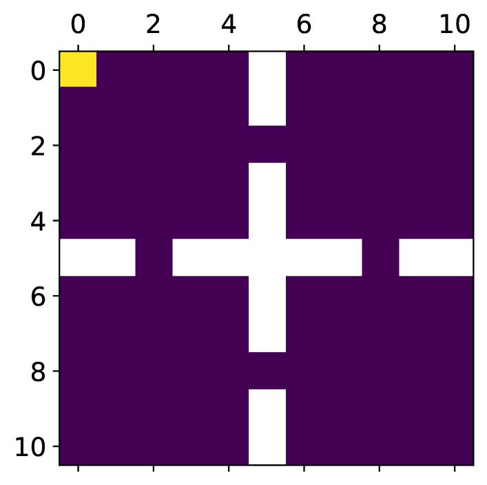
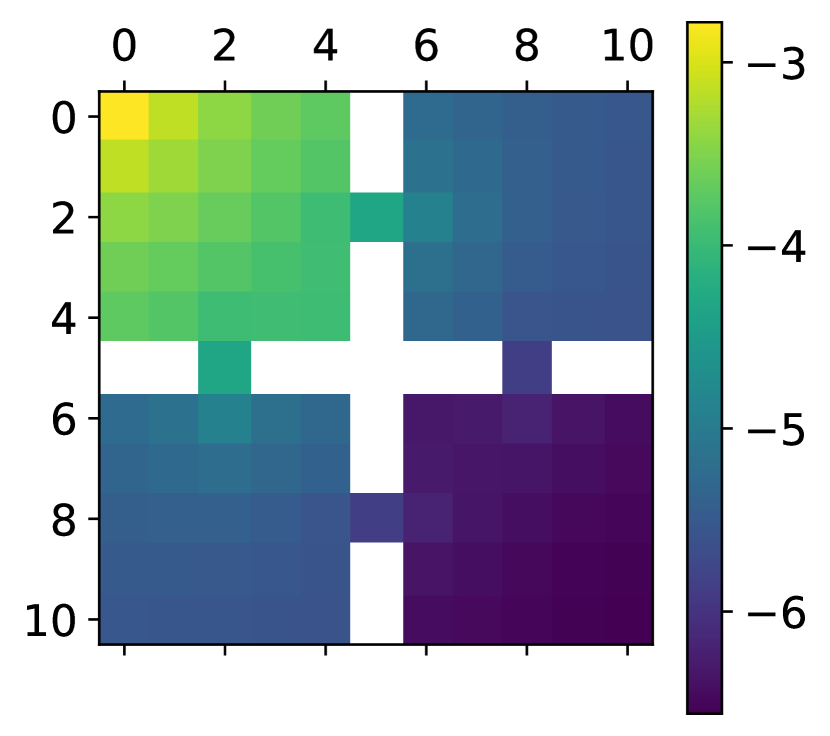
Numerical experiments.
For the sake of illustration, we now focus on the evolutive setting and compare the algorithms on the canonical example. We focus here on the exact iterative methods as described in Section 3, i.e. without RL approximations. In Figure 5, we use the notion of exploitability to check the performance of the following algorithms, which are based on the iterations described in (22):
-
•
Fixed point: is a best response against and is the mean field sequence induced by . We see that this method does not converge and the population concentrates on only a few states.
-
•
Fictitious play: As described in (37), we update the mean field by averaging over past iterations. This method converges since the exploitability goes towards . Furthermore, the final distribution is close to uniform.
-
•
Online Mirror Descent: As described in (39), the policy is updated by first computing a cumulative -function and then taking a softmax. This method converges even faster than Fictitious play, possibly because the size of each update in Fictitious play decreases with the iteration index whereas this is not the case for OMD. Accordingly, for the same number of iterations, the distribution is even closer to being uniform than with Fictitious play.
-
•
Damped Fixed Point: As described in (36), the mean field term is updated by taking the average of the previous mean field and the mean field induced by the most recent policy, with constant weights for the average. We see that the exploitability decreases but does not seem to converge, and the induced terminal distribution is not very close to uniform.
-
•
Softmax fixed point: This method is like the fixed point iterations except that the policy is a softmax of the -function instead of being an argmax as in the pure best response case. We see that the method does not converge, even though the exploitability is a bit lower than in the pure fixed point method case. The induced terminal distribution is concentrated in one of the four rooms.
-
•
Softmax fictitious play: This method is like the fictitious play iterations except that the policy is a softmax of the -function instead of being an argmax as in the pure fictitious play case. In this method, the exploitability goes down more quickly than the pure fictitious play case, as quickly as in the OMD case. However, it does not go towards . Instead, it remains roughly constant after a number of iterations. This is probably due to the regularization of the policy which prevents convergence towards the true Nash equilibrium policy. The induced terminal distribution is quite close to uniform but we see that the agents tend to avoid the walls, which is probably due to the extra regularization of the policy.
-
•
Boltzmann policy iteration: This method corresponds to the policy iteration method described in (35) except that the policy is a softmax of the -function instead of being an argmax as in the pure fictitious play case. This method does not converge as the exploitability increases to a very high level. The induced terminal distribution is concentrated in one small part of the domain.
Based on these observations, we see that a few methods are failing to converge even when using exact updates. As discussed in Section 3.4, this is probably due to the lack of contraction property for the operator on which the iterations rely.
For other methods, it is worth investigating how they perform when combined with RL as described in Section 4. The model of exploration with four rooms considered above as well as a few other examples have been treated using DRL in Laurière et al., (2022), where it is observed that a DRL versions of pure fixed point iterations still fail to converge, while a DRL version of OMD still tends to perform better than a DRL version of fictitious play. This tends to show that testing methods with exact methods before implementing DRL versions can be helpful to compare the performance of learning methods.
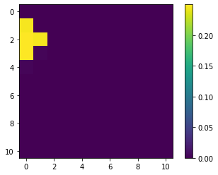
(a)
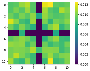
(b)
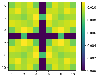
(c)
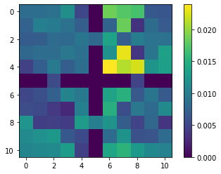
(d)
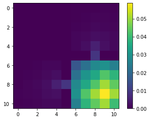
(e)
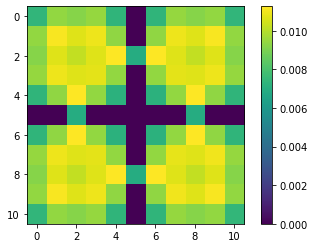
(f)
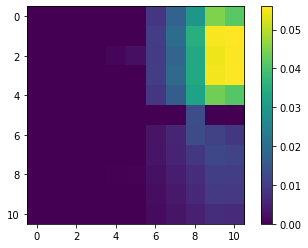
(g)
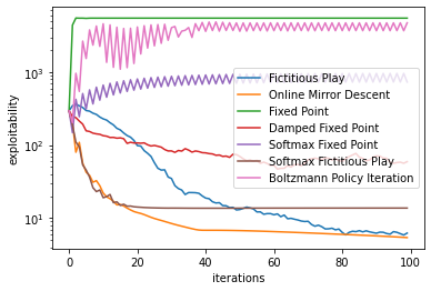
(h)
6 Conclusion and perspectives
In this work, we have surveyed some of the main recent developments related to the question of learning MFGs and MFC solutions. We first clarified the definitions of several classical settings that have appeared in the literature. As far as we know, it is the first time that these settings are summarized and discussed in comparison with each other. Second, we proposed an overview of iterative methods to learn MFG and MFC solutions by updating the mean field and the policy. Starting from simple fixed-point iterations, we explained how these procedures can be enhanced by incorporating various smoothing methods. Along the way, we clarified the link with the framework of MDPs. Third, building on this connection with MDPs, we presented RL and deep RL methods for MFGs and MFC. Finally, we provided some numerical results on a simple benchmark problem.
Several aspects were not discussed in detail here, such as:
-
•
games with multiple groups or sub-populations (Subramanian et al.,, 2018; Subramanian et al., 2020a, ; Perolat et al.,, 2021; Carmona et al.,, 2020; Yang et al.,, 2020; Cui and Koeppl, 2021b, ; Angiuli et al., 2022a, ; Mondal et al.,, 2022),
- •
-
•
games with strategic complementarities (Adlakha and Johari,, 2013; Lee et al.,, 2020; Lee et al., 2021a, ),
-
•
problems with more complex structures such as partially observable problems (Subramanian et al., 2020b, ), models with leader-follower or major-minor structures (Ghosh and Aggarwal,, 2020), and so on,
- •
-
•
other forms of RL techniques such as model-based RL (Pasztor et al.,, 2021) or inverse reinforcement learning (Yang et al., 2018a, ; Chen et al., 2021b, ; Chen et al.,, 2022).
Apart from the points covered in this survey, many directions remain to be investigated. For example, the question of approximation of the distribution has received relatively less interest than the question of approximating the policy and the value function. Efficiently representing and learning the distribution is important for mean field problems, particularly for large and complex environments for which exact tabular representations are not suitable.
Furthermore, the literature is quickly expanding in various directions and the numerical results are not always easy to compare. We hope that this survey will contribute to harmonizing the research on this topic although many aspects remain to be unified. Along these lines, having common benchmark problems and a common framework seem important. Recently, MFGs have been incorporated to the OpenSpiel library (Lanctot et al.,, 2019).111https://github.com/deepmind/open_spiel
Last but not least, one of the main motivations to use RL methods for MFGs is to be able to compute Nash equilibria at a large scale. We thus hope that the methods presented here and their extensions will find concrete applications in the near future.
Acknowledgements
The authors would like to thank their collaborators on the topic of this survey for fruitful discussions and collaborations, but also for contributions developing and maintaining the OpenSpiel code used in this survey, and in particular: Andrea Angiuli, Olivier Bachem, Theophile Cabannes, René Carmona, Gökçe Dayanikli, Romuald Élie, Jean-Pierre Fouque, Maximilien Germain, Sertan Girgin, Kenza Hamidouche, Ruimeng Hu, Ayush Jain, Marc Lanctot, Edward Lockhart, Raphael Marinier, Paul Muller, Rémi Munos, Julien Pérolat, Huyên Pham, Georgios Piliouras, Mark Rowland, Zongjun Tan, Karl Tuyls.
References
- (1) Achdou, Y., Bardi, M., and Cirant, M. (2017a). Mean field games models of segregation. Mathematical Models and Methods in Applied Sciences, 27(01).
- Achdou et al., (2014) Achdou, Y., Buera, F., Lasry, J.-M., Lions, P.-L., and Moll, B. (2014). PDE models in macroeconomics. Proceedings of the Royal Society of London. Series A, Mathematical and Physical Sciences.
- Achdou et al., (2012) Achdou, Y., Camilli, F., and Capuzzo-Dolcetta, I. (2012). Mean field games: numerical methods for the planning problem. SIAM Journal on Control and Optimization, 50(1).
- Achdou and Capuzzo-Dolcetta, (2010) Achdou, Y. and Capuzzo-Dolcetta, I. (2010). Mean field games: numerical methods. SIAM Journal on Numerical Analysis, 48(3).
- Achdou et al., (2020) Achdou, Y., Cardaliaguet, P., Delarue, F., Porretta, A., and Santambrogio, F. (2020). Mean Field Games: Cetraro, Italy 2019, volume 2281. Springer Nature.
- Achdou et al., (2016) Achdou, Y., Giraud, P.-N., Lasry, J.-M., and Lions, P.-L. (2016). A long-term mathematical model for mining industries. Applied Mathematics & Optimization, 74(3).
- (7) Achdou, Y., Han, J., Lasry, J.-M., Lions, P.-L., and Moll, B. (2017b). Income and wealth distribution in macroeconomics: A continuous-time approach. Technical report, National Bureau of Economic Research.
- Achdou and Lasry, (2019) Achdou, Y. and Lasry, J.-M. (2019). Mean field games for modeling crowd motion. In Contributions to partial differential equations and applications, pages 17–42. Springer.
- Achdou and Laurière, (2016) Achdou, Y. and Laurière, M. (2016). Mean field type control with congestion. Applied Mathematics & Optimization, 73(3).
- Achdou and Laurière, (2020) Achdou, Y. and Laurière, M. (2020). Mean field games and applications: Numerical aspects. Mean field games, pages 249–307.
- Adlakha and Johari, (2013) Adlakha, S. and Johari, R. (2013). Mean field equilibrium in dynamic games with strategic complementarities. Operations Research, 61(4):971–989.
- Alasseur et al., (2020) Alasseur, C., Taher, I. B., and Matoussi, A. (2020). An extended mean field game for storage in smart grids. Journal of Optimization Theory and Applications, 184(2).
- Anahtarci et al., (2019) Anahtarci, B., Kariksiz, C. D., and Saldi, N. (2019). Fitted Q-learning in mean-field games. arXiv preprint arXiv:1912.13309.
- Anahtarcı et al., (2019) Anahtarcı, B., Karıksız, C. D., and Saldi, N. (2019). Learning in discounted-cost and average-cost mean-field games. arXiv preprint arXiv:1912.13309.
- Anahtarci et al., (2020) Anahtarci, B., Kariksiz, C. D., and Saldi, N. (2020). Q-learning in regularized mean-field games. arXiv preprint arXiv:2003.12151.
- Anahtarcı et al., (2020) Anahtarcı, B., Karıksız, C. D., and Saldi, N. (2020). Value iteration algorithm for mean-field games. Systems & Control Letters, 143:104744.
- Anahtarci et al., (2021) Anahtarci, B., Kariksiz, C. D., and Saldi, N. (2021). Learning in discrete-time average-cost mean-field games. In 2021 60th IEEE Conference on Decision and Control (CDC), pages 3048–3053. IEEE.
- (18) Angiuli, A., Detering, N., Fouque, J.-P., and Lin, J. (2022a). Reinforcement learning algorithm for mixed mean field control games. arXiv preprint arXiv:2205.02330.
- Angiuli et al., (2021) Angiuli, A., Fouque, J.-P., and Lauriere, M. (2021). Reinforcement learning for mean field games, with applications to economics. To appear in Machine Learning And Data Sciences For Financial Markets (arXiv preprint arXiv:2106.13755).
- (20) Angiuli, A., Fouque, J.-P., and Laurière, M. (2022b). Unified reinforcement Q-learning for mean field game and control problems. Mathematics of Control, Signals, and Systems, pages 1–55.
- Angiuli et al., (2019) Angiuli, A., Graves, C. V., Li, H., Chassagneux, J.-F., Delarue, F., and Carmona, R. (2019). Cemracs 2017: numerical probabilistic approach to MFG. ESAIM: Proceedings and Surveys, 65.
- Anthony et al., (2017) Anthony, T., Tian, Z., and Barber, D. (2017). Thinking fast and slow with deep learning and tree search. In Proceedings of NeurIPS.
- Arulkumaran et al., (2017) Arulkumaran, K., Deisenroth, M. P., Brundage, M., and Bharath, A. A. (2017). Deep reinforcement learning: A brief survey. IEEE Signal Processing Magazine, 34(6):26–38.
- Aumann, (1964) Aumann, R. J. (1964). Markets with a continuum of traders. Econometrica: Journal of the Econometric Society, pages 39–50.
- Aumann and Shapley, (2015) Aumann, R. J. and Shapley, L. S. (2015). Values of non-atomic games. Princeton University Press.
- Aurell et al., (2022) Aurell, A., Carmona, R., Dayanikli, G., and Lauriere, M. (2022). Optimal incentives to mitigate epidemics: a stackelberg mean field game approach. SIAM Journal on Control and Optimization, 60(2):S294–S322.
- Aurell and Djehiche, (2019) Aurell, A. and Djehiche, B. (2019). Modeling tagged pedestrian motion: A mean-field type game approach. Transportation Research Part B: Methodological, 121.
- Bagagiolo and Bauso, (2014) Bagagiolo, F. and Bauso, D. (2014). Mean-field games and dynamic demand management in power grids. Dynamic Games and Applications, 4(2).
- Bäuerle, (2021) Bäuerle, N. (2021). Mean field Markov decision processes. arXiv preprint arXiv:2106.08755.
- (30) Bauso, D., Tembine, H., and Basar, T. (2016a). Opinion dynamics in social networks through mean-field games. SIAM Journal on Control and Optimization, 54(6).
- (31) Bauso, D., Zhang, X., and Papachristodoulou, A. (2016b). Density flow in dynamical networks via mean-field games. IEEE Transactions on Automatic Control, 62(3):1342–1355.
- Bellemare et al., (2013) Bellemare, M. G., Naddaf, Y., Veness, J., and Bowling, M. (2013). The arcade learning environment: An evaluation platform for general agents. Journal of Artificial Intelligence Research, 47:253–279.
- Bellman, (1957) Bellman, R. (1957). A Markovian decision process. Journal of mathematics and mechanics, pages 679–684.
- Bensoussan et al., (2013) Bensoussan, A., Frehse, J., Yam, P., et al. (2013). Mean field games and mean field type control theory, volume 101. Springer.
- Bensoussan et al., (2015) Bensoussan, A., Frehse, J., and Yam, S. C. P. (2015). The master equation in mean field theory. Journal de Mathématiques Pures et Appliquées, 103(6):1441–1474.
- Bensoussan et al., (2018) Bensoussan, A., Huang, T., and Laurière, M. (2018). Mean field control and mean field game models with several populations. arXiv preprint arXiv:1810.00783.
- Bertsekas, (2012) Bertsekas, D. (2012). Dynamic programming and optimal control, volume 1. Athena scientific.
- Bertsekas and Shreve, (1996) Bertsekas, D. and Shreve, S. E. (1996). Stochastic optimal control: the discrete-time case, volume 5. Athena Scientific.
- Bonnans et al., (2021) Bonnans, J. F., Lavigne, P., and Pfeiffer, L. (2021). Generalized conditional gradient and learning in potential mean field games. arXiv preprint arXiv:2109.05785.
- Borkar, (2009) Borkar, V. S. (2009). Stochastic approximation: a dynamical systems viewpoint, volume 48. Springer.
- Bowling et al., (2015) Bowling, M., Burch, N., Johanson, M., and Tammelin, O. (2015). Heads-up limit hold’em poker is solved. Science, 347(6218).
- Briceño Arias et al., (2019) Briceño Arias, L. M., Kalise, D., Kobeissi, Z., Laurière, M., Mateos González, A., and Silva, F. J. (2019). On the implementation of a primal-dual algorithm for second order time-dependent mean field games with local couplings. ESAIM: Proceedings, 65.
- Briceño Arias et al., (2018) Briceño Arias, L. M., Kalise, D., and Silva, F. J. (2018). Proximal methods for stationary mean field games with local couplings. SIAM Journal on Control and Optimization, 56(2).
- Brown, (1951) Brown, G. W. (1951). Iterative solution of games by fictitious play. Activity analysis of production and allocation, 13(1):374–376.
- Brown and Sandholm, (2017) Brown, N. and Sandholm, T. (2017). Superhuman AI for heads-up no-limit poker: Libratus beats top professionals. Science, 360(6385).
- Brown and Sandholm, (2019) Brown, N. and Sandholm, T. (2019). Superhuman AI for multiplayer poker. Science, 365(6456).
- Burger et al., (2013) Burger, M., Francesco, M., Markowich, P., and Wolfram, M.-T. (2013). Mean field games with nonlinear mobilities in pedestrian dynamics. Discrete and Continuous Dynamical Systems - Series B, 19.
- Cabannes et al., (2021) Cabannes, T., Lauriere, M., Perolat, J., Marinier, R., Girgin, S., Perrin, S., Pietquin, O., Bayen, A. M., Goubault, E., and Elie, R. (2021). Solving n-player dynamic routing games with congestion: a mean field approach. Extended abstract at AAMAS 2022 (long version: arXiv preprint arXiv:2110.11943).
- Cacace, Simone et al., (2021) Cacace, Simone, Camilli, Fabio, and Goffi, Alessandro (2021). A policy iteration method for mean field games. ESAIM: COCV, 27:85.
- Camilli and Tang, (2022) Camilli, F. and Tang, Q. (2022). Rates of convergence for the policy iteration method for mean field games systems. Journal of Mathematical Analysis and Applications, 512(1):126138.
- Campbell et al., (2002) Campbell, M., Hoane Jr, A. J., and Hsu, F.-h. (2002). Deep blue. Artificial intelligence, 134(1-2):57–83.
- Cao et al., (2020) Cao, H., Guo, X., and Laurière, M. (2020). Connecting GANs, MFGs, and OT. arXiv preprint arXiv:2002.04112.
- Cardaliaguet et al., (2019) Cardaliaguet, P., Delarue, F., Lasry, J.-M., and Lions, P. L. (2019). The master equation and the convergence problem in mean field games, volume 381 of AMS-201.
- Cardaliaguet and Hadikhanloo, (2017) Cardaliaguet, P. and Hadikhanloo, S. (2017). Learning in mean field games: the fictitious play. ESAIM Cont. Optim. Calc. Var.
- Cardaliaguet and Lehalle, (2018) Cardaliaguet, P. and Lehalle, C.-A. (2018). Mean field game of controls and an application to trade crowding. Mathematics and Financial Economics, 12(3):335–363.
- Cardaliaguet et al., (2016) Cardaliaguet, P., Porretta, A., and Tonon, D. (2016). A segregation problem in multi-population mean field games. In International Symposium on Dynamic Games and Applications. Springer.
- Carlini and Silva, (2014) Carlini, E. and Silva, F. J. (2014). A fully discrete semi-Lagrangian scheme for a first order mean field game problem. SIAM Journal on Numerical Analysis, 52(1).
- Carlini and Silva, (2015) Carlini, E. and Silva, F. J. (2015). A semi-Lagrangian scheme for a degenerate second order mean field game system. Discrete and Continuous Dynamical Systems, 35(9).
- Carmona, (2020) Carmona, R. (2020). Applications of mean field games in financial engineering and economic theory. arXiv preprint arXiv:2012.05237.
- Carmona and Delarue, (2013) Carmona, R. and Delarue, F. (2013). Mean field forward-backward stochastic differential equations. Electronic Communications in Probability, 18:1–15.
- (61) Carmona, R. and Delarue, F. (2018a). Probabilistic Theory of Mean Field Games with Applications I. Springer.
- (62) Carmona, R. and Delarue, F. (2018b). Probabilistic Theory of Mean Field Games with Applications II. Springer.
- Carmona et al., (2016) Carmona, R., Delarue, F., and Lacker, D. (2016). Mean field games with common noise. The Annals of Probability, 44(6):3740–3803.
- (64) Carmona, R., Graves, C. V., and Tan, Z. (2019a). Price of anarchy for mean field games. ESAIM: Proceedings and Surveys, 65:349–383.
- Carmona et al., (2020) Carmona, R., Hamidouche, K., Laurière, M., and Tan, Z. (2020). Policy optimization for linear-quadratic zero-sum mean-field type games. In 2020 59th IEEE Conference on Decision and Control (CDC), pages 1038–1043. IEEE.
- Carmona et al., (2021) Carmona, R., Hamidouche, K., Laurière, M., and Tan, Z. (2021). Linear-quadratic zero-sum mean-field type games: Optimality conditions and policy optimization. Journal of Dynamics & Games, 8(4):403.
- Carmona and Laurière, (2019) Carmona, R. and Laurière, M. (2019). Convergence analysis of machine learning algorithms for the numerical solution of mean field control and games: II - the finite horizon case. To appear in Annals of Applied Probability (preprint arXiv:1908.01613).
- Carmona and Laurière, (2021) Carmona, R. and Laurière, M. (2021). Convergence analysis of machine learning algorithms for the numerical solution of mean field control and games i: the ergodic case. SIAM Journal on Numerical Analysis, 59(3):1455–1485.
- (69) Carmona, R., Laurière, M., and Tan, Z. (2019b). Linear-quadratic mean-field reinforcement learning: convergence of policy gradient methods. arXiv preprint arXiv:1910.04295.
- (70) Carmona, R., Laurière, M., and Tan, Z. (2019c). Model-free mean-field reinforcement learning: mean-field MDP and mean-field Q-learning. arXiv preprint arXiv:1910.12802.
- Cecchin and Pelino, (2019) Cecchin, A. and Pelino, G. (2019). Convergence, fluctuations and large deviations for finite state mean field games via the master equation. Stochastic Processes and their Applications, 129(11):4510–4555.
- Chan and Sircar, (2015) Chan, P. and Sircar, R. (2015). Bertrand and Cournot mean field games. Applied Mathematics & Optimization, 71(3).
- Chan and Sircar, (2017) Chan, P. and Sircar, R. (2017). Fracking, renewables, and mean field games. SIAM Review, 59(3).
- Chassagneux et al., (2019) Chassagneux, J.-F., Crisan, D., and Delarue, F. (2019). Numerical method for FBSDEs of McKean–Vlasov type. The Annals of Applied Probability, 29(3):1640–1684.
- (75) Chen, M., Li, Y., Wang, E., Yang, Z., Wang, Z., and Zhao, T. (2021a). Pessimism meets invariance: Provably efficient offline mean-field multi-agent rl. Advances in Neural Information Processing Systems, 34.
- (76) Chen, Y., Liu, J., and Khoussainov, B. (2021b). Agent-level maximum entropy inverse reinforcement learning for mean field games. arXiv preprint arXiv:2104.14654.
- Chen et al., (2022) Chen, Y., Zhang, L., Liu, J., and Hu, S. (2022). Individual-level inverse reinforcement learning for mean field games. arXiv preprint arXiv:2202.06401.
- Chevalier et al., (2015) Chevalier, G., Le Ny, J., and Malhamé, R. (2015). A micro-macro traffic model based on mean-field games. In American Control Conference (ACC). IEEE.
- Cirant, (2015) Cirant, M. (2015). Multi-population mean field games systems with neumann boundary conditions. Journal de Mathématiques Pures et Appliquées, 103(5):1294–1315.
- Couillet et al., (2012) Couillet, R., Perlaza, S. M., Tembine, H., and Debbah, M. (2012). Electrical vehicles in the smart grid: A mean field game analysis. IEEE Journal on Selected Areas in Communications, 30(6).
- (81) Cui, K. and Koeppl, H. (2021a). Approximately solving mean field games via entropy-regularized deep reinforcement learning. In Banerjee, A. and Fukumizu, K., editors, Proceedings of The 24th International Conference on Artificial Intelligence and Statistics, volume 130 of Proceedings of Machine Learning Research, pages 1909–1917. PMLR.
- (82) Cui, K. and Koeppl, H. (2021b). Learning graphon mean field games and approximate Nash equilibria. arXiv preprint arXiv:2112.01280.
- Delarue and Vasileiadis, (2021) Delarue, F. and Vasileiadis, A. (2021). Exploration noise for learning linear-quadratic mean field games. arXiv preprint arXiv:2107.00839.
- (84) Djehiche, B., Tcheukam, A., and Tembine, H. (2017a). A mean-field game of evacuation in multilevel building. IEEE Transactions on Automatic Control, 62(10).
- (85) Djehiche, B., Tcheukam Siwe, A., and Tembine, H. (2017b). Mean-field-type games in engineering. AIMS Electronics and Electrical Engineering, 1.
- Doncel et al., (2022) Doncel, J., Gast, N., and Gaujal, B. (2022). A mean field game analysis of SIR dynamics with vaccination. Probability in the Engineering and Informational Sciences, 36(2):482–499.
- Duffie and Sun, (2012) Duffie, D. and Sun, Y. (2012). The exact law of large numbers for independent random matching. Journal of Economic Theory, 147(3):1105–1139.
- (88) Elie, R., Hubert, E., Mastrolia, T., and Possamaï, D. (2019a). Mean-field moral hazard for optimal energy demand response management. Mathematical Finance (to appear).
- (89) Elie, R., Hubert, E., and Turinici, G. (2020a). Contact rate epidemic control of COVID-19: an equilibrium view. Mathematical Modelling of Natural Phenomena.
- (90) Elie, R., Mastrolia, T., and Possamaï, D. (2019b). A tale of a principal and many, many agents. Mathematics of Operations Research, 44(2).
- (91) Elie, R., Perolat, J., Laurière, M., Geist, M., and Pietquin, O. (2020b). On the convergence of model free learning in mean field games. In Proceedings of the AAAI Conference on Artificial Intelligence, volume 34, pages 7143–7150.
- Feleqi, (2013) Feleqi, E. (2013). The derivation of ergodic mean field game equations for several populations of players. Dynamic Games and Applications, 3(4):523–536.
- Firoozi and Jaimungal, (2022) Firoozi, D. and Jaimungal, S. (2022). Exploratory LQG mean field games with entropy regularization. Automatica, 139:110177.
- Fouque and Zhang, (2020) Fouque, J.-P. and Zhang, Z. (2020). Deep learning methods for mean field control problems with delay. Frontiers in Applied Mathematics and Statistics, 6.
- François-Lavet et al., (2018) François-Lavet, V., Henderson, P., Islam, R., Bellemare, M. G., and Pineau, J. (2018). An introduction to deep reinforcement learning. Foundations and Trends® in Machine Learning, 11(3-4):219–354.
- Fudenberg et al., (1998) Fudenberg, D., Levine, D. K., et al. (1998). The theory of learning in games. MIT Press Books, 1.
- Fudenberg and Tirole, (1991) Fudenberg, D. and Tirole, J. (1991). Game theory. MIT press.
- Fujimoto et al., (2018) Fujimoto, S., Hoof, H., and Meger, D. (2018). Addressing function approximation error in actor-critic methods. In International Conference on Machine Learning, pages 1587–1596. PMLR.
- Gast et al., (2012) Gast, N., Gaujal, B., and Le Boudec, J.-Y. (2012). Mean field for Markov decision processes: from discrete to continuous optimization. IEEE Transactions on Automatic Control, 57(9):2266–2280.
- Geist et al., (2021) Geist, M., Pérolat, J., Laurière, M., Elie, R., Perrin, S., Bachem, O., Munos, R., and Pietquin, O. (2021). Concave utility reinforcement learning: the mean-field game viewpoint. AAMAS 2022 (arXiv preprint arXiv:2106.03787).
- Germain et al., (2022) Germain, M., Mikael, J., and Warin, X. (2022). Numerical resolution of McKean-Vlasov FBSDEs using neural networks. Methodology and Computing in Applied Probability, pages 1–30.
- Ghosh and Aggarwal, (2020) Ghosh, A. and Aggarwal, V. (2020). Model free reinforcement learning algorithm for stationary mean field equilibrium for multiple types of agents. arXiv preprint arXiv:2012.15377.
- (103) Gomes, D., Velho, R. M., and Wolfram, M.-T. (2014a). Socio-economic applications of finite state mean field games. Philosophical Transactions of the Royal Society A: Mathematical, Physical and Engineering Sciences, 372(2028).
- Gomes et al., (2010) Gomes, D. A., Mohr, J., and Souza, R. R. (2010). Discrete time, finite state space mean field games. Journal de mathématiques pures et appliquées, 93(3):308–328.
- (105) Gomes, D. A., Patrizi, S., and Voskanyan, V. (2014b). On the existence of classical solutions for stationary extended mean field games. Nonlinear Analysis: Theory, Methods & Applications, 99:49–79.
- Gomes and Saúde, (2020) Gomes, D. A. and Saúde, J. (2020). A mean-field game approach to price formation. Dynamic Games and Applications.
- Gomes and Voskanyan, (2016) Gomes, D. A. and Voskanyan, V. K. (2016). Extended deterministic mean-field games. SIAM Journal on Control and Optimization, 54(2):1030–1055.
- Goodfellow et al., (2016) Goodfellow, I., Bengio, Y., and Courville, A. (2016). Deep learning. MIT press.
- Goodfellow et al., (2014) Goodfellow, I. J., Pouget-Abadie, J., Mirza, M., Xu, B., Warde-Farley, D., Ozair, S., Courville, A., and Bengio, Y. (2014). Generative adversarial nets. In Advances in Neural Information Processing Systems 27 (NIPS).
- Graber and Bensoussan, (2018) Graber, P. J. and Bensoussan, A. (2018). Existence and uniqueness of solutions for Bertrand and Cournot mean field games. Applied Mathematics & Optimization, 77(1).
- Grover et al., (2018) Grover, P., Bakshi, K., and Theodorou, E. A. (2018). A mean-field game model for homogeneous flocking. Chaos: An Interdisciplinary Journal of Nonlinear Science, 28(6):061103.
- Gu et al., (2019) Gu, H., Guo, X., Wei, X., and Xu, R. (2019). Dynamic programming principles for mean-field controls with learning. arXiv preprint arXiv:1911.07314.
- Gu et al., (2020) Gu, H., Guo, X., Wei, X., and Xu, R. (2020). Q-learning for mean-field controls. arXiv preprint arXiv:2002.04131.
- (114) Gu, H., Guo, X., Wei, X., and Xu, R. (2021a). Mean-field controls with q-learning for cooperative marl: convergence and complexity analysis. SIAM Journal on Mathematics of Data Science, 3(4):1168–1196.
- (115) Gu, H., Guo, X., Wei, X., and Xu, R. (2021b). Mean-field multi-agent reinforcement learning: A decentralized network approach. arXiv preprint arXiv:2108.02731.
- Guéant et al., (2011) Guéant, O., Lasry, J.-M., and Lions, P.-L. (2011). Mean field games and applications. In Paris-Princeton lectures on mathematical finance 2010, pages 205–266. Springer.
- Gummadi et al., (2013) Gummadi, R., Johari, R., Schmit, S., and Yu, J. Y. (2013). Mean field analysis of multi-armed bandit games. Available at SSRN 2045842.
- Guo et al., (2019) Guo, X., Hu, A., Xu, R., and Zhang, J. (2019). Learning mean-field games. Advances in Neural Information Processing Systems, 32.
- (119) Guo, X., Hu, A., Xu, R., and Zhang, J. (2020a). A general framework for learning mean-field games. arXiv preprint arXiv:2003.06069.
- (120) Guo, X., Xu, R., and Zariphopoulou, T. (2020b). Entropy regularization for mean field games with learning. arXiv preprint arXiv:2010.00145.
- Hadikhanloo, (2017) Hadikhanloo, S. (2017). Learning in anonymous nonatomic games with applications to first-order mean field games. arXiv preprint arXiv:1704.00378.
- Hadikhanloo, (2018) Hadikhanloo, S. (2018). Learning in mean field games. PhD thesis, PhD thesis. Université Paris sciences et lettres.
- Hadikhanloo and Silva, (2019) Hadikhanloo, S. and Silva, F. J. (2019). Finite mean field games: fictitious play and convergence to a first order continuous mean field game. Journal de Mathématiques Pures et Appliquées, 132:369–397.
- Hamidouche et al., (2016) Hamidouche, K., Saad, W., Debbah, M., and Poor, H. V. (2016). Mean-field games for distributed caching in ultra-dense small cell networks. In 2016 American Control Conference (ACC). IEEE.
- Hu, (2021) Hu, R. (2021). Deep fictitious play for stochastic differential games. Communications in mathematical sciences, 19(2).
- Hu and Laurière, (2022) Hu, R. and Laurière, M. (2022). Recent developments in machine learning methods for stochastic control and games. SSRN preprint:4096569.
- Huang et al., (2017) Huang, K., Di, X., Du, Q., and Chen, X. (2017). A game-theoretic framework for autonomous vehicles velocity control: Bridging microscopic differential games and macroscopic mean field games. Discrete & Continuous Dynamical Systems - B, 22(11).
- Huang et al., (2019) Huang, K., Di, X., Du, Q., and Chen, X. (2019). Stabilizing traffic via autonomous vehicles: A continuum mean field game approach. In 2019 IEEE Intelligent Transportation Systems Conference (ITSC), pages 3269–3274. IEEE.
- Huang et al., (2006) Huang, M., Malhamé, R. P., and Caines, P. E. (2006). Large population stochastic dynamic games: closed-loop McKean-Vlasov systems and the Nash certainty equivalence principle. Communications in Information & Systems, 6(3):221–252.
- Hubert and Turinici, (2018) Hubert, E. and Turinici, G. (2018). Nash-MFG equilibrium in a SIR model with time dependent newborn vaccination. Ricerche di Matematica, 67(1).
- Iyer et al., (2014) Iyer, K., Johari, R., and Sundararajan, M. (2014). Mean field equilibria of dynamic auctions with learning. Management Science, 60(12):2949–2970.
- Kizilkale et al., (2019) Kizilkale, A. C., Salhab, R., and Malhamé, R. P. (2019). An integral control formulation of mean field game based large scale coordination of loads in smart grids. Automatica, 100.
- Kobeissi, (2022) Kobeissi, Z. (2022). On classical solutions to the mean field game system of controls. Communications in Partial Differential Equations, 47(3):453–488.
- Kolokoltsov and Bensoussan, (2016) Kolokoltsov, V. N. and Bensoussan, A. (2016). Mean-field-game model for botnet defense in cyber-security. Applied Mathematics & Optimization, 74(3).
- Kolokoltsov and Malafeyev, (2018) Kolokoltsov, V. N. and Malafeyev, O. A. (2018). Corruption and botnet defense: a mean field game approach. International Journal of Game Theory, 47(3).
- Koutsoupias and Papadimitriou, (1999) Koutsoupias, E. and Papadimitriou, C. (1999). Worst-case equilibria. In Annual symposium on theoretical aspects of computer science, pages 404–413. Springer.
- Lachapelle et al., (2016) Lachapelle, A., Lasry, J.-M., Lehalle, C.-A., and Lions, P.-L. (2016). Efficiency of the price formation process in presence of high frequency participants: a mean field game analysis. Mathematics and Financial Economics, 10(3).
- Lacker, (2017) Lacker, D. (2017). Limit theory for controlled McKean–Vlasov dynamics. SIAM Journal on Control and Optimization, 55(3):1641–1672.
- Lacker, (2020) Lacker, D. (2020). On the convergence of closed-loop Nash equilibria to the mean field game limit. The Annals of Applied Probability, 30(4):1693–1761.
- Lacker and Ramanan, (2019) Lacker, D. and Ramanan, K. (2019). Rare Nash equilibria and the price of anarchy in large static games. Mathematics of Operations Research, 44(2):400–422.
- Laguzet and Turinici, (2015) Laguzet, L. and Turinici, G. (2015). Individual vaccination as Nash equilibrium in a SIR model with application to the 2009–2010 influenza A (H1N1) epidemic in France. Bulletin of Mathematical Biology, 77(10):1955–1984.
- Lanctot et al., (2019) Lanctot, M., Lockhart, E., Lespiau, J.-B., Zambaldi, V., Upadhyay, S., Pérolat, J., Srinivasan, S., Timbers, F., Tuyls, K., Omidshafiei, S., et al. (2019). Openspiel: A framework for reinforcement learning in games. arXiv preprint arXiv:1908.09453.
- Lanctot et al., (2009) Lanctot, M., Waugh, K., Zinkevich, M., and Bowling, M. (2009). Monte carlo sampling for regret minimization in extensive games. volume 22, pages 1078–1086.
- Lasry and Lions, (2007) Lasry, J.-M. and Lions, P.-L. (2007). Mean field games. Japanese Journal of Mathematics, 2(1).
- Lauriere, (2021) Lauriere, M. (2021). Numerical methods for mean field games and mean field type control. Mean Field Games, 78:221.
- Laurière et al., (2022) Laurière, M., Perrin, S., Girgin, S., Muller, P., Jain, A., Cabannes, T., Piliouras, G., Pérolat, J., Élie, R., Pietquin, O., et al. (2022). Scalable deep reinforcement learning algorithms for mean field games. arXiv preprint arXiv:2203.11973.
- Laurière et al., (2021) Laurière, M., Song, J., and Tang, Q. (2021). Policy iteration method for time-dependent mean field games systems with non-separable hamiltonians. arXiv preprint arXiv:2110.02552.
- (148) Lee, K., Rengarajan, D., Kalathil, D., and Shakkottai, S. (2021a). Reinforcement learning for mean field games with strategic complementarities. In International Conference on Artificial Intelligence and Statistics, pages 2458–2466. PMLR.
- Lee et al., (2020) Lee, K.-Y., Rengarajan, D., Kalathil, D. M., and Shakkottai, S. (2020). Learning trembling hand perfect mean field equilibrium for dynamic mean field games. CoRR.
- (150) Lee, W., Liu, S., Tembine, H., Li, W., and Osher, S. (2021b). Controlling propagation of epidemics via mean-field control. SIAM Journal on Applied Mathematics, 81(1):190–207.
- Li et al., (2016) Li, F., Malhamé, R. P., and Le Ny, J. (2016). Mean field game based control of dispersed energy storage devices with constrained inputs. In 2016 IEEE 55th Conference on Decision and Control (CDC). IEEE.
- Li et al., (2021) Li, Y., Wang, L., Yang, J., Wang, E., Wang, Z., Zhao, T., and Zha, H. (2021). Permutation invariant policy optimization for mean-field multi-agent reinforcement learning: A principled approach. arXiv preprint arXiv:2105.08268.
- Lillicrap et al., (2016) Lillicrap, T. P., Hunt, J. J., Pritzel, A., Heess, N., Erez, T., Tassa, Y., Silver, D., and Wierstra, D. (2016). Continuous control with deep reinforcement learning. In ICLR (Poster).
- Lin et al., (2020) Lin, A. T., Fung, S. W., Li, W., Nurbekyan, L., and Osher, S. J. (2020). APAC-Net: Alternating the population and agent control via two neural networks to solve high-dimensional stochastic mean field games. arXiv preprint arXiv:2002.10113.
- Lions, (2012) Lions, P.-L. (2006-2012). Lecture at the collège de france.
- Maghsudi and Hossain, (2017) Maghsudi, S. and Hossain, E. (2017). Distributed user association in energy harvesting dense small cell networks: A mean-field multi-armed bandit approach. IEEE Access, 5:3513–3523.
- McAleer et al., (2020) McAleer, S., Lanier, J., Fox, R., and Baldi, P. (2020). Pipeline PSRO: A scalable approach for finding approximate Nash equilibria in large games. In Proceedings of NeurIPS.
- Mériaux et al., (2012) Mériaux, F., Varma, V., and Lasaulce, S. (2012). Mean field energy games in wireless networks. In 2012 Conference Record of the Forty Sixth Asilomar Conference on Signals, Systems and Computers (ASILOMAR). IEEE.
- Meyn, (2022) Meyn, S. (2022). Control Systems and Reinforcement Learning. Cambridge University Press.
- Mguni et al., (2018) Mguni, D., Jennings, J., and Munoz de Cote, E. (2018). Decentralised learning in systems with many, many strategic agents. In Proceedings of AAAI.
- Miehling et al., (2022) Miehling, E., Başar, T., et al. (2022). Reinforcement learning for non-stationary discrete-time linear–quadratic mean-field games in multiple populations. Dynamic Games and Applications, pages 1–47.
- Mishra et al., (2020) Mishra, R. K., Vasal, D., and Vishwanath, S. (2020). Model-free reinforcement learning for non-stationary mean field games. In 2020 59th IEEE Conference on Decision and Control (CDC), pages 1032–1037. IEEE.
- Mitchell et al., (1997) Mitchell, T. M. et al. (1997). Machine learning.
- Mnih et al., (2013) Mnih, V., Kavukcuoglu, K., Silver, D., Graves, A., Antonoglou, I., Wierstra, D., and Riedmiller, M. (2013). Playing atari with deep reinforcement learning. arXiv preprint arXiv:1312.5602.
- Mondal et al., (2022) Mondal, W. U., Agarwal, M., Aggarwal, V., and Ukkusuri, S. V. (2022). On the approximation of cooperative heterogeneous multi-agent reinforcement learning (marl) using mean field control (mfc). Journal of Machine Learning Research, 23(129):1–46.
- Moravčík et al., (2017) Moravčík, M., Schmid, M., Burch, N., Lisỳ, V., Morrill, D., Bard, N., Davis, T., Waugh, K., Johanson, M., and Bowling, M. (2017). Deepstack: Expert-level artificial intelligence in heads-up no-limit poker. Science, 356(6337):508–513.
- Motte and Pham, (2019) Motte, M. and Pham, H. (2019). Mean-field Markov decision processes with common noise and open-loop controls. arXiv preprint arXiv:1912.07883.
- Muller et al., (2021) Muller, P., Rowland, M., Elie, R., Piliouras, G., Perolat, J., Lauriere, M., Marinier, R., Pietquin, O., and Tuyls, K. (2021). Learning equilibria in mean-field games: Introducing mean-field psro. AAMAS 2022 (arXiv preprint arXiv:2111.08350).
- Nash, (1951) Nash, J. (1951). Non-cooperative games. Annals of mathematics, pages 286–295.
- Nash, (1950) Nash, J. F. (1950). Equilibrium points in n-person games. Proceedings of the national academy of sciences, 36(1):48–49.
- Nourian et al., (2010) Nourian, M., Caines, P. E., and Malhamé, R. P. (2010). Synthesis of cucker-smale type flocking via mean field stochastic control theory: Nash equilibria. In 2010 48th Annual Allerton Conference on Communication, Control, and Computing (Allerton), pages 814–819. IEEE.
- Nourian et al., (2011) Nourian, M., Caines, P. E., and Malhamé, R. P. (2011). Mean field analysis of controlled cucker-smale type flocking: Linear analysis and perturbation equations. IFAC Proceedings Volumes, 44(1):4471–4476.
- Papamakarios et al., (2021) Papamakarios, G., Nalisnick, E., Rezende, D. J., Mohamed, S., and Lakshminarayanan, B. (2021). Normalizing flows for probabilistic modeling and inference. Journal of Machine Learning Research, 22(57):1–64.
- Parise et al., (2015) Parise, F., Grammatico, S., Gentile, B., and Lygeros, J. (2015). Network aggregative games and distributed mean field control via consensus theory. arXiv preprint arXiv:1506.07719.
- Pasztor et al., (2021) Pasztor, B., Bogunovic, I., and Krause, A. (2021). Efficient model-based multi-agent mean-field reinforcement learning. arXiv preprint arXiv:2107.04050.
- Perolat et al., (2021) Perolat, J., Perrin, S., Elie, R., Laurière, M., Piliouras, G., Geist, M., Tuyls, K., and Pietquin, O. (2021). Scaling up mean field games with online mirror descent. AAMAS 2022 (arXiv preprint arXiv:2103.00623).
- (177) Perrin, S., Laurière, M., Pérolat, J., Élie, R., Geist, M., and Pietquin, O. (2021a). Generalization in mean field games by learning master policies. AAAI’22 (arXiv preprint arXiv:2109.09717).
- (178) Perrin, S., Laurière, M., Pérolat, J., Geist, M., Élie, R., and Pietquin, O. (2021b). Mean field games flock! the reinforcement learning way. IJCAI 2021 (arXiv preprint arXiv:2105.07933).
- Perrin et al., (2020) Perrin, S., Pérolat, J., Laurière, M., Geist, M., Elie, R., and Pietquin, O. (2020). Fictitious play for mean field games: Continuous time analysis and applications. In proc. of NeurIPS.
- Puterman, (2014) Puterman, M. L. (2014). Markov decision processes: discrete stochastic dynamic programming. John Wiley & Sons.
- Rezende and Mohamed, (2015) Rezende, D. and Mohamed, S. (2015). Variational inference with normalizing flows. In International conference on machine learning, pages 1530–1538. PMLR.
- Robinson, (1951) Robinson, J. (1951). An iterative method of solving a game. Annals of mathematics, pages 296–301.
- Roughgarden and Tardos, (2007) Roughgarden, T. and Tardos, E. (2007). Introduction to the inefficiency of equilibria. Algorithmic game theory, 17:443–459.
- Ruthotto et al., (2020) Ruthotto, L., Osher, S. J., Li, W., Nurbekyan, L., and Fung, S. W. (2020). A machine learning framework for solving high-dimensional mean field game and mean field control problems. Proceedings of the National Academy of Sciences, 117(17).
- Salhab et al., (2018) Salhab, R., Le Ny, J., and Malhamé, R. P. (2018). A mean field route choice game model. In 2018 IEEE Conference on Decision and Control (CDC), pages 1005–1010. IEEE.
- Samarakoon et al., (2015) Samarakoon, S., Bennis, M., Saad, W., Debbah, M., and Latva-Aho, M. (2015). Energy-efficient resource management in ultra dense small cell networks: A mean-field approach. In IEEE Global Communications Conference (GLOBECOM).
- Samuel, (1959) Samuel, A. L. (1959). Some studies in machine learning using the game of checkers. IBM Journal of Research and Development, 3(3).
- Schaeffer et al., (2007) Schaeffer, J., Burch, N., Björnsson, Y., Kishimoto, A., Müller, M., Lake, R., Lu, P., and Sutphen, S. (2007). Checkers is solved. Science, 317(5844).
- Schmeidler, (1973) Schmeidler, D. (1973). Equilibrium points of nonatomic games. Journal of statistical Physics, 7(4):295–300.
- Shannon, (1959) Shannon, C. E. (1959). Programming a computer playing chess. Philosophical Magazine, Ser.7, 41(312).
- Shiri et al., (2019) Shiri, H., Park, J., and Bennis, M. (2019). Massive autonomous UAV path planning: A neural network based mean-field game theoretic approach. In IEEE Global Communications Conference (GLOBECOM).
- Silver et al., (2016) Silver, D., Huang, A., Maddison, C. J., Guez, A., Sifre, L., Van Den Driessche, G., Schrittwieser, J., Antonoglou, I., Panneershelvam, V., Lanctot, M., et al. (2016). Mastering the game of Go with deep neural networks and tree search. Nature, 529(7587).
- Silver et al., (2018) Silver, D., Hubert, T., Schrittwieser, J., Antonoglou, I., Lai, M., Guez, A., Lanctot, M., Sifre, L., Kumaran, D., Graepel, T., Lillicrap, T., Simonyan, K., and Hassabis, D. (2018). A general reinforcement learning algorithm that masters chess, shogi, and Go through self-play. Science, 632(6419).
- Silver et al., (2017) Silver, D., Schrittwieser, J., Simonyan, K., Antonoglou, I., Huang, A., Guez, A., Hubert, T., Baker, L., Lai, M., Bolton, A., et al. (2017). Mastering the game of Go without human knowledge. Nature, 550(7676).
- Stella et al., (2013) Stella, L., Bagagiolo, F., Bauso, D., and Como, G. (2013). Opinion dynamics and stubbornness through mean-field games. In 52nd IEEE Conference on Decision and Control. IEEE.
- Subramanian and Mahajan, (2019) Subramanian, J. and Mahajan, A. (2019). Reinforcement learning in stationary mean-field games. In Proceedings of the 18th International Conference on Autonomous Agents and MultiAgent Systems, pages 251–259.
- Subramanian et al., (2018) Subramanian, J., Seraj, R., and Mahajan, A. (2018). Reinforcement learning for mean-field teams. In Workshop on Adaptive and Learning Agents at International Conference on Autonomous Agents and Multi-Agent Systems.
- (198) Subramanian, S. G., Poupart, P., Taylor, M. E., and Hegde, N. (2020a). Multi type mean field reinforcement learning. arXiv preprint arXiv:2002.02513.
- (199) Subramanian, S. G., Taylor, M. E., Crowley, M., and Poupart, P. (2020b). Partially observable mean field reinforcement learning. CoRR, abs/2012.15791.
- Sun, (2006) Sun, Y. (2006). The exact law of large numbers via Fubini extension and characterization of insurable risks. Journal of Economic Theory, 126(1):31–69.
- Sutton and Barto, (2018) Sutton, R. S. and Barto, A. G. (2018). Reinforcement Learning: An Introduction. The MIT Press, 2nd edition.
- Szepesvári, (2010) Szepesvári, C. (2010). Algorithms for reinforcement learning. Synthesis lectures on artificial intelligence and machine learning, 4(1):1–103.
- Sznitman, (1991) Sznitman, A.-S. (1991). Topics in propagation of chaos. In Ecole d’été de probabilités de Saint-Flour XIX—1989, pages 165–251. Springer.
- Tanaka et al., (2020) Tanaka, T., Nekouei, E., Pedram, A. R., and Johansson, K. H. (2020). Linearly solvable mean-field traffic routing games. IEEE Transactions on Automatic Control, 66(2):880–887.
- Tembine et al., (2012) Tembine, H., Tempone, R., and Vilanova, P. (2012). Mean-field learning: a survey. arXiv preprint arXiv:1210.4657.
- uz Zaman et al., (2020) uz Zaman, M. A., Zhang, K., Miehling, E., and Ba\textcommabelowsar, T. (2020). Reinforcement learning in non-stationary discrete-time linear-quadratic mean-field games. In 2020 59th IEEE Conference on Decision and Control (CDC), pages 2278–2284. IEEE.
- Vinyals et al., (2019) Vinyals, O., Babuschkin, I., Czarnecki, W. M., Mathieu, M., Dudzik, A., Chung, J., Choi, D. H., Powell, R., Ewalds, T., Georgiev, P., et al. (2019). Grandmaster level in starcraft ii using multi-agent reinforcement learning. Nature, 575(7782):350–354.
- Wang et al., (2020) Wang, L., Yang, Z., and Wang, Z. (2020). Breaking the curse of many agents: Provable mean embedding q-iteration for mean-field reinforcement learning. In International Conference on Machine Learning, pages 10092–10103. PMLR.
- Wang et al., (2021) Wang, W., Han, J., Yang, Z., and Wang, Z. (2021). Global convergence of policy gradient for linear-quadratic mean-field control/game in continuous time. In International Conference on Machine Learning, pages 10772–10782. PMLR.
- Wang et al., (2022) Wang, X., Cerny, J., Li, S., Yang, C., Yin, Z., Chan, H., and An, B. (2022). A unified perspective on deep equilibrium finding. arXiv preprint arXiv:2204.04930.
- Wang and Jia, (2021) Wang, X. and Jia, R. (2021). Mean field equilibrium in multi-armed bandit game with continuous reward. arXiv preprint arXiv:2105.00767.
- Watkins, (1989) Watkins, C. (1989). Learning form delayed rewards. Ph. D. thesis, King’s College, University of Cambridge.
- Watkins and Dayan, (1992) Watkins, C. J. and Dayan, P. (1992). Q-learning. Machine learning, 8(3-4):279–292.
- Williams, (1992) Williams, R. J. (1992). Simple statistical gradient-following algorithms for connectionist reinforcement learning. Machine learning, 8(3):229–256.
- Xie et al., (2021) Xie, Q., Yang, Z., Wang, Z., and Minca, A. (2021). Learning while playing in mean-field games: Convergence and optimality. In Meila, M. and Zhang, T., editors, Proceedings of the 38th International Conference on Machine Learning, volume 139 of Proceedings of Machine Learning Research, pages 11436–11447. PMLR.
- Yang et al., (2017) Yang, C., Li, J., Sheng, M., Anpalagan, A., and Xiao, J. (2017). Mean field game-theoretic framework for interference and energy-aware control in 5G ultra-dense networks. IEEE Wireless Communications, 25(1).
- Yang et al., (2020) Yang, F., Vereshchaka, A., Chen, C., and Dong, W. (2020). Bayesian multi-type mean field multi-agent imitation learning. Advances in Neural Information Processing Systems, 33:2469–2478.
- (218) Yang, J., Ye, X., Trivedi, R., Xu, H., and Zha, H. (2018a). Learning deep mean field games for modeling large population behavior. In International Conference on Learning Representations.
- (219) Yang, Y., Luo, R., Li, M., Zhou, M., Zhang, W., and Wang, J. (2018b). Mean field multi-agent reinforcement learning. In Proceedings of ICML.
- Yang and Wang, (2020) Yang, Y. and Wang, J. (2020). An overview of multi-agent reinforcement learning from game theoretical perspective. arXiv preprint arXiv:2011.00583.
- Zhang et al., (2021) Zhang, K., Yang, Z., and Başar, T. (2021). Multi-agent reinforcement learning: A selective overview of theories and algorithms. Handbook of Reinforcement Learning and Control, pages 321–384.
- Zinkevich et al., (2007) Zinkevich, M., Johanson, M., Bowling, M., and Piccione, C. (2007). Regret minimization in games with incomplete information. volume 20, pages 1729–1736.