A Critical Compilation of Experimental Data on the 1s2$l$2$l^{\prime}$ Core-Excited States of Li-like Ions from Carbon to Uranium

Recent advance in calculations of energy levels of the 1s2$l$2$l^{\prime}$ core-excited states for ions along the Li isoelectronic sequence from carbon to uranium suggested that theoretical predictions for the 1s${}^{2}2l$-1s2$l$2$l^{\prime}$ transitions are significantly more precise than most of the experimental results available today and can thus be used for calibrating measured X-ray spectra. This suggestion is verified in the present work by comparison with benchmark experimental results. We present a critical compilation of all available experimental data on the energy levels of the 1s2$l$2$l^{\prime}$ core-excited states of Li-like ions. The compiled experimental data include uncertainty estimates, which allowed proper weighted averaging and comparison with theoretical calculations. This comparison confirmed the supremacy of the most advanced theoretical calculations of the 1s2$l$2$l^{\prime}$ levels over the best experimental results available today.

Contentstoc

ldt

ldf

1 Introduction

Dielectronic satellite spectra of highly charged ions are an important source of spectroscopic data widely used for analyzing astrophysical plasmas as well as spectra from electron beam ion traps, tokamaks and laser-produced plasmas (see, e.g., [1, 2, 3, 4]). Such spectra provide crucial information on the electron temperature and density, the ionization state distribution, and other characteristics of hot plasmas. An analysis of such spectra requires detailed knowledge of energy levels of various excited states of highly charged ions. High-quality energies (theoretical or experimental) are critical for a proper fit of spectral line profiles and thus for a better plasma diagnostic.

A significant progress in theory of highly charged ions has been achieved in the last years. For Li-like ions, new advanced theoretical studies provided energies with estimations of uncertainties due to effects that are not included in previous calculations [5, 6]. For the core-excited states of these ions, these theoretical predictions were shown to be significantly (by an order of magnitude) more precise than the best experimental energies available today. This conclusion was based on a comparison of theoretical values with benchmark experimental results for several atomic numbers $Z$ in the region from $Z=6$ to $Z=80$ and for several different experiments. In the study by Yerokhin et al. [5, 6], energy levels and fine-structure intervals of the 1s2$l$2$l^{\prime}$ core-excited states were calculated for ions along the Li isoelectronic sequence from carbon to uranium. All theoretical energies were supplied with uncertainty estimates.

The goal of the present work is to extend a collection of benchmark experimental results used for the verification of the theoretical calculations in Refs. [5, 6] to all available experimental data on the 1s2$l$2$l^{\prime}$ core-excited states for ions along the Li isoelectronic sequence, and to compare these data with the theoretical results obtained in Refs. [5, 6]. Validation of both the calculated energies and their uncertainties is our task. If the correctness of the statement about precision of the theoretical predictions is confirmed on all available experimental data, high-precision theoretical energies of core-excited states of Li-like ions published in Refs. [5, 6] may become the preferable source of spectroscopic data for modeling plasma spectra and may be used for calibration of experimental X-ray spectra of ions with a larger number of electrons.

In this work, when discussing the satellite structures near the resonance lines of He-like ions, we use the designations of Gabriel [7] (a, b, c, etc.) for transitions forming these structures. Translation of these designations to standard spectroscopic notation of transitions will be discussed in the following Section.

2 Coupling schemes

When reading the literature on the core-excited levels of Li-like ions, one faces a difficulty with heterogeneous spectroscopic notation. In the early papers [8, 7] dealing with moderately charged ions, a peculiar kind of $LS$-coupling scheme was used to designate the 1s2s², 1s2p², and 1s2s2p energy levels, which we will call Gabriel’s scheme. For the 1s2p² configuration having two equivalent p-electrons it is impossible to distinguish between them, so the two p-electrons are combined first to produce an intermediate singlet (¹S or ¹D) or triplet (³P) term, which is then combined with the ²S term of the 1s shell to produce the final $LS$ term. For the odd 1s2s2p configuration, Gabriel’s coupling scheme first combines the 1s and 2p electron to produce an intermediate ¹P^∘ or ³P^∘, which then are combined with the remaining 2s electron to obtain the final doublet and quartet $LS$-terms. In many subsequent studies (see, e.g., Vainshtein and Safronova [9]), a ‘reordered’ $LS$-coupling was used, in which the two $n=2$ electrons are combined first, and then the intermediate singlet and quartet terms are combined with the 1s-electron. Other researchers (see, e.g., Chen [10]) used a ‘sequential’ $LS$-coupling, in which the electronic subshells are combined in the order of their binding energy, i.e., first 1s is combined with 2s, and then the 2p subshell is added. We put the word ‘sequential’ in quotes, because, as mentioned above, the 1s2p² configuration must be an exception: the two 2p-electrons are indistinguishable and thus must be combined first, same as in Gabriel’s scheme. Further advancement of both theory and experiments into the region of very high nuclear charges $Z$ led to realization that at high $Z$ the coupling changes to $jj$, which also has many different versions. Most relativistic atomic-structure codes have only a ‘sequential’ $jj$-coupling option (with the same exception for the 1s2p² configuration). However, Cowan’s codes [11, 12], while making all calculations in $LS$-coupling, have an option to transform the output to $jj$-coupling, as well as several other coupling schemes, with a given order of summation of subshells. For subshells with equivalent electrons, such as 2p², these codes can only compute the $LS$-coupling level composition.

Yerokhin et al. [5, 6] did not provide percentage composition of their calculated energy levels. To designate the levels, for all $Z$ they used the same ‘sequential’ $LS$-coupling labels as in C IV ($Z=6$). In Section 4 of Ref. [6] the authors mentioned in passing that at high $Z$ the levels structure approaches the $jj$-coupling limit. However, the choice of a physically appropriate coupling scheme for each $Z$ was, to our knowledge, never discussed in the literature. To illustrate the problem, we depicted their scaled energies of the 1s2s2p and 1s2p² configurations in Fig. 1. For the scaling, the energies counted from the lowest level of each configuration were divided by the energy spread of that configuration in each ion. The figure clearly shows that, indeed, the coupling conditions change drastically from the low-$Z$ to high-$Z$ end of the sequence. One can hardly expect the $LS$-coupling labels given by Yerokhin and Surzhykov [6] to have much physical meaning for Li-like uranium. The level labels used in Fig. 1 are explained below.

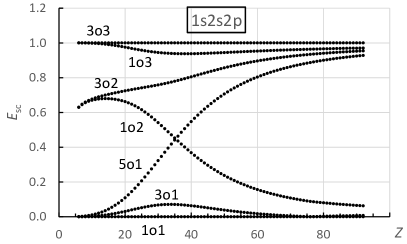
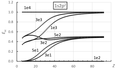
Fig. 1: Energy structure of the 1s2s2p (left) and 1s2p² (right) configurations of Li-like ions as a function of nuclear charge $Z$. $E_{\text{sc}}$ is the energy separation from the lowest level of each configuration divided by the energy spread of that configuration in each ion. For explanation of level labels, see text.

The smoothness of all energy-level dependencies on $Z$ seen in Fig. 1 suggests that, in the context of isoelectronic comparisons, the energy is a crucial part of the level identity. The dominant $LS$- or $jj$-coupling character of a level may change with $Z$, but we found that the energy order of levels within each $J^{\pi}$ set (where $J$ is the total angular momentum quantum number and $\pi$ is the parity) is preserved for the entire isoelectronic sequence. Therefore, we chose to designate the levels with labels constructed from three symbols: an integer number equal to $2J$ followed by a parity symbol (‘e’ for even and ‘o’ for odd) followed by sequential number of the level in the order of increasing energies in each $J^{\pi}$ set. The numbering starts with zero in the sets that include 1s²2$l$ levels and from 1 otherwise, so that the first core-excited level in each set has the number 1 in its label. These labels are used in Fig. 1 and in all other figures and tables, as well as the main text.

To determine the best coupling scheme describing the level structure for each ion, we calculated percentage compositions of levels in the ‘sequential’ and ‘reordered’ $LS$- and $jj$-coupling schemes for $Z=6$, 18, 26, 34, 42, 54, 68, 80, and 92. The ‘sequential’ $jj$-coupling calculations were made with the Flexible Atomic Code (FAC) code [13], while the ‘reordered’ $jj$-coupling, as well as ’sequential’ and ‘reordered’ $LS$-coupling calculations were made with Cowan’s codes [11, 12]. In the Cowan-code calculations, only the 1s²2s, 1s²2p, 1s2s², 1s2s2p, and 1s2p² configurations were included, and the Slater parameters were varied in the least-squares fitting procedure to fit the level values given by Yerokhin et al. [5, 6]. The FAC calculations additionally included the 1s${}^{2}nl$ ($n=3$, 4, 5, $l\leq n-1$), 1s(2s+2p)$nl$ ($n=3$, 4, $l\leq n-1$), and 1s(3s+3p+3d)² configurations (38 configurations in total). The only output in common to the two sets of calculations was the percentage composition in the ‘sequential’ $jj$-coupling for the 1s2s2p configuration. For this configuration, the two sets of our results for percentage composition were found to agree within 2.4 % on average.

The change in composition of the 1s2s2p and 1s2p² levels along the sequence in the ‘reordered’ $LS$-coupling scheme is illustrated in Fig. 2. This figure shows only the levels with the most drastic changes. For even parity, there are only two levels with $J=5/2$, so only one plot is shown. The plot for the other $J=5/2$ level, 5e2, looks exactly the same with the labels interchanged. It is these two levels, 5e1 and 5e2, that set the upper limit ($Z\leq 38$) for applicability of $LS$ coupling labels to the $n=2$ core-excited levels in Li-like ions. In odd parity, switching of the leading $LS$ components of the 3o2 and 3o3 levels happens at much greater $Z$, near $Z=60$.

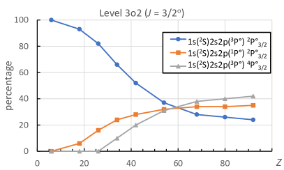
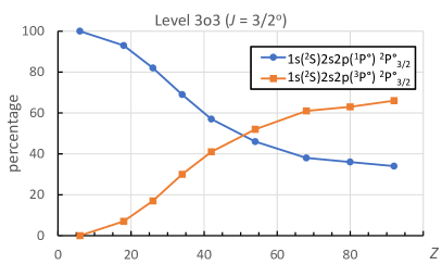
Fig. 2: Percentages of the eigenvector components in the composition of two 1s2s2p $J=3/2$ levels (top) and one 1s2p² $J=5/2$ level (bottom) of Li-like ions as a function of nuclear charge $Z$. The ‘reordered’ $LS$ coupling was used to construct the basis sets (see text).

Behavior of the $jj$-coupling level compositions that most drastically change along the isoelectronic sequence is shown in Fig. 3. The average purity of eigenvectors (i.e., mean percentage of the leading component) in ‘sequential’ $jj$ coupling at $Z=92$ was found to be 98 % (odd parity) and 88 % (even parity). Even at $Z=34$ the $jj$ purity is higher than in the $LS$ coupling: it is 90 % (odd) and 84 % (even), while in $LS$ it is 89 % (odd) and 80 % (even). However, in the context of isoelectronic comparisons, it is not the purity that determines the best coupling scheme. It is rather the constancy of the dominant eigenvector component associated with each level. From this point of view, as can be seen in Fig. 3, the $jj$ coupling has a disadvantage in the medium-$Z$ region. The two even-parity $J=3/2$ levels, 3e1 and 3e2 (bottom of Fig. 3) change their leading component. For the level 3e1, this change occurs at $Z\approx 53$, while the level 3e2 changes its leading component twice: at $Z\approx 18$ and at $Z\approx 53$.

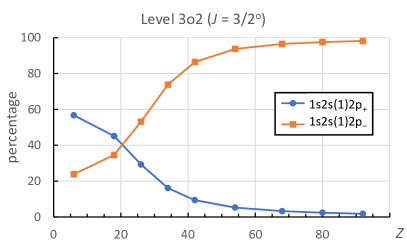
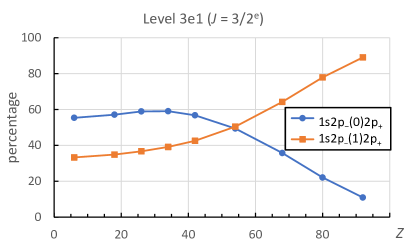
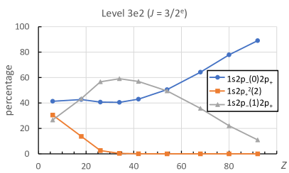
Fig. 3: Percentages of the eigenvector components in the composition of one 1s2s2p $J=3/2$ level (top left), one 1s2p² $J=5/2$ level (top right), and two 1s2p² $J=3/2$ levels (bottom) of Li-like ions as a function of nuclear charge $Z$. The ‘sequential’ $jj$ coupling was used to construct the basis sets (see text).

From this point of view, the best coupling scheme describing the 1s2s2p and 1s2p² levels of Li-like ions with low and moderate $Z$ is the ‘reordered’ $LS$ coupling (with the two $n=2$ electrons combined first to each other and then to 1s). It provides the highest average purity of level composition (100 % for odd parity and 98 % for even parity) at $Z=6$. The dominant components of the eigenvectors remain the same (with percentages greater than 50 %) up to $Z=38$. For higher $Z$, physically more adequate level labels are provided by the ‘sequential’ $jj$-coupling scheme, which has the highest purity of the eigenvectors at $Z=92$ (98 % for odd parity and 88 % for even parity) compared to all other schemes we tested.

The level labels to be used in the ranges of $Z$ specified above are listed in Table A.

Table A: Level labels. $LS$ labels are valid for $Z\leq 38$, while $jj$ labels are valid for higher $Z$ (see text). Energy values ($E$) are quoted from Yerokhin et al. [5, 6] for guidance to energy ordering. The column ‘Lbl’ contains labels referred to in other tables of this paper (see text).

Lbl	$Z=6$		$Z=92$
	$E$, cm-1 [5]	$LS$ label	$E$, cm-1 [6]	$jj$ label
1e0	0	1s22s 2S	0	1s22s
1e1	2351890	1s2s2 2S	773422346	1s2s2
1e2	2446336	1s2p2 4P	776509696	1s2p${}_{-}^{2}$(0)
1e3	2481997	1s2p2 2P	810836077	1s2p-(1)2p+
1e4	2521456	1s2p2 2S	846376043	1s2p${}_{+}^{2}$(0)
3e1	2446412	1s2p2 4P	810528593	1s2p-(1)2p+
3e2	2472063	1s2p2 2D	811560453	1s2p-(0)2p+
3e3	2482143	1s2p2 2P	846069107	1s2p${}_{+}^{2}$(2)
5e1	2446451	1s2p2 4P	810374741	1s2p-(1)2p+
5e2	2471954	1s2p2 2D	845332989	1s2p${}_{+}^{2}$(2)
1o0	64483	1s22p 2P∘	2264603	1s22p-
1o1	2371985	1s(2S)2s2p(3P∘) 4P∘	774051580	1s2s(1)2p-
1o2	2419321	1s(2S)2s2p(3P∘) 2P∘	776112227	1s2s(0)2p-
1o3	2447237	1s(2S)2s2p(1P∘) 2P∘	809788085	1s2s(1)2p+
3o0	64588	1s22p 2P∘	35968939	1s22p+
3o1	2371989	1s(2S)2s2p(3P∘) 4P∘	773775700	1s2s(1)2p-
3o2	2419419	1s(2S)2s2p(3P∘) 2P∘	809179263	1s2s(1)2p+
3o3	2447226	1s(2S)2s2p(1P∘) 2P∘	810879642	1s2s(0)2p+
5o1	2372086	1s(2S)2s2p(3P∘) 4P∘	808211489	1s2s(1)2p+

Throughout this paper, we use letter labels to denote the $n=2\rightarrow n=1$ satellite transitions of Li-like ions and the nearby transitions of He-like ions. Translation of these labels to the spectroscopic designations of the lower and upper levels of the transitions is given in Table B. Most of these labels were defined by Gabriel [7]. The forbidden transition labels E and U were introduced by Beier and Kunze [14].

Table B: Classification of satellite transitions near resonance transitions of He-like ions in the $LS$ and $jj$ coupling schemes. The first column contains transition labels, most of which were defined by Gabriel [7]. The numbers 1 and 2 in the column headings refer to the lower and upper levels of the transitions. The columns ‘Lbl1’ and ‘Lbl2’ refer to the column ‘Lbl’ of Table A. For transitions in Li-like ions, the $LS$-coupling labels are applicable to $Z\leq 38$, while the $jj$-coupling labels are applicable for higher $Z$ (see text). Either $LS$- or $jj$-labels unambiguously define the levels of transitions in He-like ions in the entire sequence.

Label	Lbl1	Lbl2	Level1 ($LS$)	Level2 ($LS$)	Level1 ($jj$)	Level2 ($jj$)
a	3o0	3e3	1s22p 2P${}^{\circ}_{3/2}$	1s2p2 2P3/2	(1s22p+)3/2	[1s2p${}_{+}^{2}$(2)]3/2
b	1o0	3e3	1s22p 2P${}^{\circ}_{1/2}$	1s2p2 2P3/2	(1s22p-)1/2	[1s2p${}_{+}^{2}$(2)]3/2
c	3o0	1e3	1s22p 2P${}^{\circ}_{3/2}$	1s2p2 2P1/2	(1s22p+)3/2	[1s2p-(1)2p+]1/2
d	1o0	1e3	1s22p 2P${}^{\circ}_{1/2}$	1s2p2 2P1/2	(1s22p-)1/2	[1s2p-(1)2p+]1/2
e	3o0	5e1	1s22p 2P${}^{\circ}_{3/2}$	1s2p2 4P5/2	(1s22p+)3/2	[1s2p-(1)2p+]5/2
E	1o0	5e1	1s22p 2P${}^{\circ}_{1/2}$	1s2p2 4P5/2	(1s22p-)1/2	[1s2p-(1)2p+]5/2
f	3o0	3e1	1s22p 2P${}^{\circ}_{3/2}$	1s2p2 4P3/2	(1s22p+)3/2	[1s2p-(1)2p+]3/2
g	1o0	3e1	1s22p 2P${}^{\circ}_{1/2}$	1s2p2 4P3/2	(1s22p-)1/2	[1s2p-(1)2p+]3/2
h	3o0	1e2	1s22p 2P${}^{\circ}_{3/2}$	1s2p2 4P1/2	(1s22p+)3/2	[1s2p${}_{-}^{2}$(0)]1/2
i	1o0	1e2	1s22p 2P${}^{\circ}_{1/2}$	1s2p2 4P1/2	(1s22p-)1/2	[1s2p${}_{-}^{2}$(0)]1/2
j	3o0	5e2	1s22p 2P${}^{\circ}_{3/2}$	1s2p2 2D5/2	(1s22p+)3/2	[1s2p${}_{+}^{2}$(2)]5/2
k	1o0	3e2	1s22p 2P${}^{\circ}_{1/2}$	1s2p2 2D3/2	(1s22p-)1/2	[1s2p-(0)2p+]3/2
l	3o0	3e2	1s22p 2P${}^{\circ}_{3/2}$	1s2p2 2D3/2	(1s22p+)3/2	(1s2p-(0)2p+)3/2
m	3o0	1e4	1s22p 2P${}^{\circ}_{3/2}$	1s2p2 2S1/2	(1s22p+)3/2	[1s2p${}_{+}^{2}$(0)]1/2
n	1o0	1e4	1s22p 2P${}^{\circ}_{1/2}$	1s2p2 2S1/2	(1s22p-)1/2	[1s2p${}_{+}^{2}$(0)]1/2
o	3o0	1e1	1s22p 2P${}^{\circ}_{3/2}$	1s2s2 2S1/2	(1s22p+)3/2	(1s2s2)1/2
p	1o0	1e1	1s22p 2P${}^{\circ}_{1/2}$	1s2s2 2S1/2	(1s22p-)1/2	(1s2s2)1/2
q	1e0	3o2	1s22s 2S1/2	1s(2S)2s2p(3P∘) 2P${}^{\circ}_{3/2}$	(1s22s)1/2	[1s2s(1)2p+]3/2
r	1e0	1o2	1s22s 2S1/2	1s(2S)2s2p(3P∘) 2P${}^{\circ}_{1/2}$	(1s22s)1/2	[1s2s(0)2p-]1/2
s	1e0	3o3	1s22s 2S1/2	1s(2S)2s2p(1P∘) 2P${}^{\circ}_{3/2}$	(1s22s)1/2	[1s2s(0)2p+]3/2
t	1e0	1o3	1s22s 2S1/2	1s(2S)2s2p(1P∘) 2P${}^{\circ}_{1/2}$	(1s22s)1/2	[1s2s(1)2p+]1/2
u	1e0	3o1	1s22s 2S1/2	1s(2S)2s2p(3P∘) 4P${}^{\circ}_{3/2}$	(1s22s)1/2	[1s2s(1)2p-]3/2
U	1e0	5o1	1s22s 2S1/2	1s(2S)2s2p(3P∘) 4P${}^{\circ}_{5/2}$	(1s22s)1/2	[1s2s(1)2p+]5/2
v	1e0	1o1	1s22s 2S1/2	1s(2S)2s2p(3P∘) 4P${}^{\circ}_{1/2}$	(1s22s)1/2	[1s2s(1)2p-]1/2
w			1s2 1S0	1s2p 1P${}^{\circ}_{1}$	(1s2)0	(1s2p+)1
x			1s2 1S0	1s2p 3P${}^{\circ}_{2}$	(1s2)0	(1s2p+)2
y			1s2 1S0	1s2p 3P${}^{\circ}_{1}$	(1s2)0	(1s2p-)1
z			1s2 1S0	1s2s 3S1	(1s2)0	(1s2s)1

$LS$- and $jj$-coupling percentage compositions of the Li-like ion levels calculated in this work for $Z=6$, 18, 26, 34, 42, 54, 68, 80, and 92 are given in Tables LABEL:table:composition_LS and LABEL:table:composition_jj, respectively.

Table C: Percentage composition of the levels of Li-like ions in the ‘reordered’ $LS$ coupling scheme from the present calculations. The top row specifies the nuclear charge $Z$. The basis states corresponding to the labels in column Lbl are given in the column of $Z=6$ of Table A. The leading percentage in the compositions given for each ion corresponds to the label given in the first column, unless it is followed by a label of another basis state. Contributions of one or two other basis states are specified as well, if they are 1 % or greater.

Lbl	6	18	26	34	42	54	68	80	92
1e0	100	100	100	100	100	100	100	100	100
1e1	91 + 9 1e4	93 + 7 1e4	94 + 5 1e4	95 + 4 1e4	94 + 4 1e4	96 + 2 1e4	96 + 2 1e4	96 + 2 1e4	87 + 6 1e2 + 5 1e4
1e2	100	99	94 + 4 1e4	79 + 12 1e4 + 7 1e3	63 + 20 1e4 + 13 1e3	52 + 27 1e4 + 18 1e3	47 + 29 1e4 + 20 1e3	45 + 30 1e4 + 20 1e3	41 + 28 1e4 + 19 1e3
1e3	100	99	93 + 4 1e4	83 + 13 1e2	75 + 23 1e2	70 + 30 1e2	68 + 32 1e2	68 + 32 1e2	67 + 33 1e2
1e4	91 + 9 1e1	92 + 7 1e1	87 + 5 1e3	80 + 10 1e3 + 8 1e2	74 + 13 1e2 + 12 1e3	71 + 17 1e2 + 12 1e3	69 + 20 1e2 + 12 1e3	68 + 21 1e2 + 11 1e3	67 + 21 1e2 + 11 1e3
3e1	100	100	98	96 + 2 3e2	93 + 4 3e2	91 + 6 3e2	89 + 7 3e2	89 + 8 3e2	89 + 6 3e2 + 5 3e3
3e2	100	94 + 6 3e3	79 + 21 3e3	70 + 29 3e3	66 + 33 3e3	63 + 37 3e3	61 + 38 3e3	60 + 39 3e3	61 + 39 3e3
3e3	100	94 + 6 3e2	79 + 20 3e2	69 + 27 3e2	64 + 30 3e2 + 6 3e1	60 + 32 3e2 + 9 3e1	58 + 32 3e2 + 10 3e1	57 + 33 3e2 + 10 3e1	56 + 33 3e2 + 10 3e1
5e1	100	99	87 + 13 5e2	62 + 38 5e2	53 5e2 + 47 5e1	61 5e2 + 39 5e1	64 5e2 + 36 5e1	65 5e2 + 35 5e1	65 5e2 + 35 5e1
5e2	100	99	87 + 13 5e1	62 + 38 5e1	53 5e1 + 47 5e2	61 5e1 + 39 5e2	64 5e1 + 36 5e2	65 5e1 + 35 5e2	65 5e1 + 35 5e2
1o0	100	100	100	100	100	100	100	100	100
1o1	100	100	99	97 + 2 1o3	95 + 3 1o3	92 + 4 1o3	91 + 6 1o3	90 + 6 1o3	90 + 7 1o3
1o2	100	100	98 + 2 1o3	90 + 10 1o3	83 + 16 1o3	78 + 22 1o3	75 + 24 1o3	75 + 25 1o3	74 + 25 1o3
1o3	100	100	98 + 2 1o2	89 + 9 1o2	81 + 15 1o2	74 + 19 1o2 + 7 1o1	70 + 21 1o2 + 9 1o1	69 + 21 1o2 + 10 1o1	68 + 22 1o2 + 10 1o1
3o0	100	100	100	100	100	100	100	100	100
3o1	100	100	97 + 2 3o3	89 + 7 3o3	78 + 15 3o3 + 7 3o2	67 + 23 3o3 + 9 3o2	61 + 28 3o3 + 10 3o2	59 + 30 3o3 + 11 3o2	58 + 32 3o3 + 11 3o2
3o2	100	93 + 6 3o3	82 + 16 3o3	66 + 24 3o3 + 10 3o1	52 + 28 3o3 + 20 3o1	39 + 31 3o1 + 30 3o3	38 3o1 + 34 3o3 + 28 3o2	40 3o1 + 34 3o3 + 26 3o2	42 3o1 + 35 3o3 + 24 3o2
3o3	100	93 + 7 3o2	82 + 17 3o2	69 + 30 3o2	57 + 41 3o2	52 3o2 + 46 3o3	61 3o2 + 38 3o3	63 3o2 + 36 3o3	66 3o2 + 34 3o3
5o1	100	100	100	100	100	100	100	100	100

Table C: (continued)

Table D: Percentage composition of the levels of Li-like ions in the ‘sequential’ $jj$-coupling scheme from the present calculations. The basis states corresponding to the labels in column Lbl are given in the column of $Z=92$ of Table A.

Lbl	6	18	26	34	42	54	68	80	92
1e0	100	100	100	100	100	100	100	100	100
1e1	89 + 7 1e4 + 3 1e2	91 + 5 1e4 + 4 1e2	92 + 4 1e2 + 4 1e4	94 + 4 1e2 + 2 1e4	94 + 5 1e2 + 1 1e4	95 + 5 1e2	95 + 5 1e2	95 + 5 1e2	95 + 5 1e2
1e2	43 + 34 1e3 + 22 1e4	51 + 30 1e3 + 19 1e4	66 + 21 1e3 + 12 1e4	84 + 8 1e3 + 5 1e4	92 + 4 1e1 + 2 1e3	94 + 5 1e1	95 + 5 1e1	95 + 5 1e1	95 + 5 1e1
1e3	65 + 23 1e2 + 12 1e4	69 + 25 1e2 + 6 1e4	78 + 20 1e2 + 1 1e4	91 + 8 1e2	97 + 2 1e2	100	100	100	100
1e4	59 + 30 1e2 + 10 1e1	70 + 21 1e2 + 9 1e1	83 + 10 1e2 + 6 1e1	93 + 3 1e2 + 3 1e1	97 + 1 1e1 + 1 1e2	99	100	100	100
3e1	55 3e2 + 33 3e1 + 11 3e3	57 3e2 + 35 3e1 + 8 3e3	59 3e2 + 37 3e1 + 4 3e3	59 3e2 + 39 3e1 + 2 3e3	57 3e2 + 43 3e1 + 1 3e3	50 + 49 3e2	64 + 36 3e2	78 + 22 3e2	89 + 11 3e2
3e2	41 + 31 3e3 + 27 3e1	43 3e1 + 43 3e2 + 14 3e3	57 3e1 + 41 3e2 + 3 3e3	59 3e1 + 41 3e2	57 3e1 + 43 3e2	51 + 49 3e1	64 + 36 3e1	78 + 22 3e1	89 + 11 3e1
3e3	58 + 39 3e1 + 2 3e2	78 + 22 3e1	93 + 7 3e1	98 + 2 3e1	99	100	100	100	100
5e1	65 5e2 + 34 5e1	55 5e2 + 45 5e1	70 + 30 5e2	92 + 8 5e2	98 + 2 5e2	100	100	100	100
5e2	65 5e1 + 34 5e2	55 5e1 + 45 5e2	70 + 30 5e1	92 + 8 5e1	98 + 2 5e1	100	100	100	100
1o0	99	100	100	100	100	100	100	100	100
1o1	88 + 11 1o3	91 + 9 1o3	94 + 6 1o3	97 + 3 1o3	98 + 1 1o3 + 1 1o2	98 + 2 1o2	97 + 3 1o2	95 + 5 1o2	93 + 7 1o2
1o2	57 + 38 1o3 + 5 1o1	67 + 30 1o3 + 3 1o1	85 + 15 1o3	95 + 5 1o3	98 + 2 1o3	98 + 2 1o1	97 + 3 1o1	95 + 5 1o1	93 + 7 1o1
1o3	50 + 42 1o2 + 6 1o1	61 + 33 1o2 + 6 1o1	79 + 15 1o2 + 5 1o1	92 + 5 1o2 + 3 1o1	97 + 1 1o1 + 1 1o2	99	100	100	100
3o0	99	100	100	100	100	100	100	100	100
3o1	55 + 44 3o2	62 + 38 3o2	73 + 26 3o2	87 + 13 3o2	95 + 5 3o2	99 + 1 3o2	100	100	100
3o2	57 3o3 + 24 3o2 + 19 3o1	45 3o3 + 35 3o2 + 20 3o1	53 + 29 3o3 + 18 3o1	74 + 16 3o3 + 10 3o1	86 + 9 3o3 + 4 3o1	94 + 5 3o3 + 1 3o1	97 + 3 3o3	98 + 2 3o3	98 + 2 3o3
3o3	43 + 31 3o2 + 25 3o1	55 + 27 3o2 + 18 3o1	71 + 20 3o2 + 9 3o1	84 + 13 3o2 + 3 3o1	90 + 8 3o2 + 1 3o1	95	97 + 3 3o2	98 + 2 3o2	98 + 2 3o2
5o1	99	100	100	100	100	100	100	100	100

Table D: (continued)

3 Collection and evaluation of experimental data

Our collection of experimental data includes absolute measurements of excitation energies for the levels of 1s2$l$2$l^{\prime}$ core-excited states [15, 16, 17, 14, 18, 19, 20, 21, 22, 23, 24, 25, 26, 27, 28, 29, 30, 31, 32, 33, 34, 35, 36, 37, 38, 39, 40, 41, 42, 43, 44, 45, 46, 8, 47, 48, 49, 50, 51, 52, 53, 54, 55, 56, 57, 58, 59, 60, 61, 62, 63, 64, 65, 66, 67, 68, 69, 70, 71, 72, 73, 74, 75, 76, 77, 78, 79, 80, 81, 82, 83, 84, 85, 86, 87, 88, 89, 90, 91, 92, 93, 94, 95, 96, 97, 98, 99, 100, 101, 102, 103, 104, 105], as well as relative measurements of the fine structure and term separations from 1s2s2p ⁴P^∘ [106, 107, 108, 109, 110, 111, 112, 113]. Our aim is to collect and review all available experimental data related to energy levels of the 1s2$l$2$l^{\prime}$ core-excited configurations in Li-like ions. The criteria for data to be included in our collection for comparison with theory are (i) availability of estimations of uncertainties of experimental energies and (ii) reasonably small deviations of energies obtained in the given experiment from those obtained in other experiments, as well as from theoretical predictions. Unfortunately, many studies, especially those published 40 years ago or earlier, either do not include estimations of measurement uncertainties or provide too rough estimations. For such works, we tried to estimate uncertainties by considering the number of decimals in the values published, comparing the results presented with other data obtained by the same group and/or on a similar experimental setup, by verifying the calibration standards and methods used, and/or by other methods.

Another problem we ran into is that many studies had used outdated reference data to calibrate the experimental setup. Those data, which include experimental and theoretical energies of levels and transitions, often turned out to be corrected in later publications. For such works, we adjusted the measured energies and/or corrected the related uncertainties.

For some studies, a review of the experiment and the data obtained shows that calibration of the experimental setup was done inaccurately or not quite correctly: the number of the standards used was too small, they did not cover the entire range of the experimental results, and/or the complexity of the calibration curve did not correspond to the number and the range of standards used. Where possible, we corrected the calibration curve used in the experiment, adjusted the experimental energies and/or revised the related uncertainties of energy values. All uncertainties given in the current study are on the level of one standard deviation.

In many studies, spectral resolution was insufficient to resolve components of multiple blended transitions. In some of these studies, the centers of gravity of the unresolved blends were measured very precisely, but the separation between the unresolved components was much larger than the measurement precision. This was the case, e.g., in the work of Hell et al. [53] on the spectra of Si and S. For the Si q+r blend, the statistical uncertainty (on the 1$\sigma$ level, reduced from their reported value on the 90 % confidence level) was 0.00011 Å, while the theoretical separation between q and r is 0.00200 Å [6]. If we use the reported central wavelength to derive the upper energy levels, 1s(²S)2s2p(³P^∘) ²P${}^{\circ}_{1/2,3/2}$ (levels 1o2 and 3o2, see Table A) of these two transitions, they would have the same value that strongly differs from theory, giving a wrong indication of a failure of theory. One way to deal with this is to compare not the energy levels derived from experiments, but the directly measured line positions. However, this would require a derivation of the corresponding theoretical positions for centers of blended lines. This, in turn, would require knowledge of relative intensities of all blended transitions. The latter strongly depend on plasma conditions that are not precisely known in most experiments. Furthermore, it would greatly increase the number of quantities used in comparisons, as in different experiments there are different blended transitions, and decrease the statistics of data available for comparison for each quantity. All experimental data involving blended transitions are for $Z\leq 29$, where the energy structure is described by the $LS$ coupling sufficiently well (see the previous Section). Therefore, in the present work we derive the energy levels of precisely measured blended transitions by assuming the theoretical separation between fine-structure components of $LS$ terms as calculated by Yerokhin et al. [5, 6]. If the observed blends involve transitions from different terms, we increase the measurement uncertainties according to theoretical separations between the terms.

In Refs. [18, 19, 24, 30, 31, 42, 44, 75, 91, 92, 98, 99], all experimental measurements were made relative to the resonance line w (1s^2 1S₀ – 1s2p ¹P${}^{\circ}_{1}$) or intercombination line y (1s^2 1S₀ – 1s2p ³P${}^{\circ}_{1}$) of the corresponding helium-like ions. Many of these measurements also used the lines x (1s^2 1S₀ – 1s2p ³P${}^{\circ}_{2}$) and z (1s^2 1S₀ – 1s2s ³S₁) for calibration. Reference wavelengths of these lines were taken from other experimental or theoretical studies. In 2005, after these articles had been published, Artemyev et al. [114] presented refined calculations of energy levels for the $n=1$ and $n=2$ states of He-like ions with nuclear charge in the range from $Z=12$ to $Z=100$. A significant improvement in precision of theoretical predictions was achieved, especially in the high-$Z$ region. For $Z<12$, theoretical wavelengths of Yerokhin and Surzhykov [115] are presently considered to be the most precise ones. They agree well with those of Drake [116] but, unlike the latter, they are accompanied by well determined small uncertainties. The calculated wavelengths of Refs. [114, 115, 116] are in good agreement with experimental data, with the calculated uncertainties provided being generally much smaller than the experimental ones. This good agreement with a large body of experimental data was recently convincingly demonstrated by Indelicato [117]. Therefore, we adjusted experimental data from the articles quoted above to the wavelengths of the lines w, x, y, and z taken from Ref. [115] for $Z<12$ and from Ref. [114] for $Z\geq 12$.

In 1942, Flemberg [45] calibrated his curved-crystal spectrograph with characteristic X-ray lines of various chemical elements. At that time, reference wavelengths of these lines were expressed in the so-called X units (X.U.). To convert the measured wavelengths to Å units, he used the relation 1000.00 X.U. = 1.00200 Å. In 1973, 31 years later, Deslattes and Henins [118] corrected this relation to 1000.00 X.U. = 1.0020802 Å. As a result, all Flemberg’s wavelengths given in angstroms are in error by roughly a factor of 1.0020802/1.00200 = 1.00008004. We analyzed Flemberg’s data for each of the elements studied (F, Mg, and Al) and determined the exact scaling factors for his X units by taking a weighted average for the particular reference lines he used, taking as standards the modern data on characteristic lines from Deslattes et al. [119]. These factors turned out to be 1.0020758(11) for F, 1.002073(7) for Mg, and 1.002078(6) for Al. The systematic uncertainties stemming from uncertainties of those scaling factors were taken into account in the derivation of energy levels from Flemberg’s corrected data.

Aglitskii et al. [16] and Boiko et al. [25] used Flemberg’s original (uncorrected) wavelengths expressed in angstroms as standards. Therefore, their wavelengths should be scaled by roughly a factor of 1.00008004. Besides that, in both these studies the experimental wavelengths of the He-like lines w and y differ notably from the much more precise theoretical values given by Artemyev et al. [114] and by Yerokhin and Surzhykov [115]. To take this into account, we recalibrated all their reported wavelengths using the reference data from the above sources, as well as the reference wavelengths for the H-like Ly$\alpha$ lines from Yerokhin and Shabaev [120]. For higher members of the H-like resonance series, we used the reference data from the Atomic Spectra Database (ASD) [15] of the National Institute of Standards and Technology (NIST).

Parkinson [75] reported high-resolution X-ray measurements of emission from solar active regions made with three rocket-borne crystal spectrometers. This study includes many lines of several spectra, including Ne-like Fe XVII and Ni XIX, as well as F-like Fe XVIII, so we found it important to analyse these data in detail. We re-calibrated Parkinson’s reported wavelengths for each crystal separately by using precise theoretical wavelengths of resonance lines of H-like and He-like Ne, Na, and Mg [120, 115, 15]. For the ADP and gypsum crystals, it was found appropriate to make additive corrections of $-0.0013(4)$ Å and $+0.0012(8)$ Å, respectively, where the values in parentheses (0.4 mÅ and 0.8 mÅ) represent the uncertainties of the weighted least-squares fit. For the KAP crystal, we found a linear correction amounting to $-0.0080(10)$ Å at 9.177 Å, $-0.0005(7)$ Å at 12.51 Å, $+0.0095(15)$ Å at 17.041 Å, and $+0.0207(27)$ Å at 22.07 Å. The uncertainties of the least-squares fit of this correction can be approximated by a cubic polynomial. We found that the statistical uncertainties for unblended lines are about 0.0012 Å for the ADP crystal and 0.0025 Å for both the gypsum and KAP crystals below 14 Å. For the region between 14 Å and 15.2 Å recorded with the KAP crystal, the measurements are hopelessly spoiled by an inexplicable distortion of the dispersion curve. For longer wavelengths, the statistical uncertainties of the corrected KAP measurements increase from 0.003 Å at (15.259–17.086) Å to 0.007 Å at (18–19) Å and 0.010 Å above that. For blended lines, such as the j and k lines in Li-like Mg X, which are on a shoulder of the much stronger z line, the statistical uncertainties specified above must be doubled. For this compilation, we derived the energy of the 1s(²S)2s2p(³P^∘) ²P^∘ term of Ne VIII from a weighted mean of the unresolved q and r satellites in the gypsum and KAP crystal spectra. For Mg X, only the ADP crystal measurements were used, since the gypsum and KAP spectra appear to have a much lower resolution.

One of the purposes of the work by Kononov et al. [60] was to experimentally observe, measure, and interpret the satellite structure near the Fe XXV resonance lines. The wavelength-measurement uncertainty of spectral lines was stated to be 0.0003 Å. The lines of interest for the present study are in the range of (1.85–1.88) Å. A comparison of the measured wavelengths of the w and y lines with the values given by Artemyev et al. [114] showed a difference of about $-0.0006$ Å and 0.0003 Å, respectively. In the initial analysis, we assumed that all identifications given by Kononov et al. are correct. Under this assumption, disagreement between the values of the 1s²2p ²P^∘ $J=3/2$–1/2 fine-structure splitting derived from several pairs of observed lines prompted us to double the wavelength uncertainties. However, a closer examination showed that this disagreement is due to several incorrect identifications. Kononov et al. [60] based their identifications on the old calculations of Vainshtein and Safronova (see references in [60]). Those theoretical wavelengths are systematically lower than the much more precise ones calculated in Refs. [114, 6] by 0.00047(9) Å. This systematic error is comparable in size with separations between the observed lines. Thus, it was easy to misidentify the lines. For example, the line observed at 1.8552 Å was interpreted as the Li-like satellite s. Based on the new calculations quoted above, we have identified it as the He-like 1s^{2 1}S₀ – 1s2p ³P${}^{\circ}_{2}$ forbidden transition (x in Gabriel’s designations [7]), while the neighboring line at 1.8563 Å has been re-interpreted as a blend of the s and m satellite transitions. Similarly, the line at 1.8678 Å has been re-interpreted as a blend of the Li-like satellite l and the He-like forbidden transition z (1s^{2 1}S₀ – 1s2p ³S₁). Assignments of the satellite transitions q, e, and u have been moved from the lines at 1.8604 Å, 1.8721 Å, and 1.8730 Å to those at 1.8614 Å, 1.8730 Å, and 1.8739 Å, respectively. We also added an assignment of the satellite transition b to the previous classification of the line at 1.8580 Å. After these revisions, all observed wavelength intervals appear to be statistically consistent with the wavelength uncertainty of 0.0003 Å stated by Kononov et al. [60]. However, we increased it to (0.0004–0.0006) Å for multiply classified lines where the relative intensities of the contributing transitions are not known. We have derived the Fe XXIV energy levels from the original observed wavelengths of Kononov et al. with our revised classifications by using the least-squares level optimization code LOPT [121] and used them in the present analysis.

Bombarda et al. [26] observed the spectrum of Li-like Ni in the vicinity of the He-like resonance line w with a carefully characterized crystal spectrometer. These observations were made in emission of the JET tokamak. The relative positions of the reported lines were stated to be accurate to about 0.0001 Å. By comparing the reported wavelengths of the He-like lines w, x, y, and z with the reference values of Artemyev et al. [114], we determined that the reported wavelengths must be shifted by a constant correction of 0.00017(6) Å. This correction was used to derive the experimental energy levels reported here. In addition to He- and Li-like lines, Bombarda et al. reported observed wavelengths of three lines of Be-like Ni. Their corrected wavelengths are 1.60444(11) Å, 1.60884(11) Å, and 1.61084(11) Å.

In the study by Safronova and Sidelnikov [86], Ni spectra were investigated in the region of (1.58–1.61) Å. Uncertainties of the wavelength measurements were not specified. However, the measurements were made with the same quartz crystal spectrometer and with the same calibration method as in Ref. [60], and thus the same uncertainty of 0.0003 Å can be expected for unblended lines. We analyzed the data of Ref. [86] by comparing them with theoretical values of Artemyev et al. [114] and of Yerokhin and Surzhykov [6] in the same way as described above for Ref. [60]. In addition, we used the wavelengths of three lines of Be-like Ni observed by Bombarda et al. [26] and corrected by us as described above. It turned out that many of the line classifications given in Ref. [86] must be revised. In particular, the three Be-like lines mentioned above were mis-identified, and the line assigned to the g satellite must have been blended with the He-like z line. The revisions of the He-like satellite assignments are straightforward, as they are based on matching the observed wavelengths with the theoretical ones from the above references. By comparing the reported wavelengths of the He-like w and y lines with the reference theoretical values [114] and the wavelengths of the three Be-like lines with the more precise experimental values described above, we determined that there is a significant systematic shift well described by a quadratic polynomial. To derive the Ni XXVI energy levels from the data of Ref.  [86], we used our revised classifications and removed the systematic shift. Its uncertainty was added in quadrature to the statistical uncertainties.

In the study of He- and Li-like Mo by Beier and Kunze [14], an ingenious technique of noise suppression by analyzing correlations of intensities recorded in several spectrograms was used. The uncertainties of the reported wavelengths were specified as $\pm$0.0002 Å. Beier and Kunze stated that theoretical wavelengths they used to identify the observed lines are accurate to $\pm$0.0005 Å. They referred to Ivanov et al. [122]. However, that paper was about He-like ions only. For He-like Mo, indeed, the reference wavelengths used by Beier and Kunze agree with those of Ref. [114] within $\pm$0.0003 Å. However, for Li-like Mo, the theoretical wavelengths of Goldsmith [123] (which were used by Beier and Kunze) differ from those of Yerokhin and Surzhykov [6] by $\pm$0.003 Å on average. As a result, some of the line identifications of Beier and Kunze had to be revised. We dropped both classifications of the line observed at 0.6859 Å, as their new theoretical wavelengths are too far from the observed one. Assignment of the r satellite transition has been moved from the line observed at 0.6885 Å to 0.6928 Å. Assignment of the s satellite transition has been dropped from the line at 0.6893 Å. Assignments of the t, q, and U satellite transitions have been added to the multiple classifications of the lines at 0.6885 Å, 0.6893 Å, and 0.6912 Å, respectively. The precise positions of the lines depicted in Figure 4 of Beier and Kunze [14] were determined by digitizing this figure and establishing a quadratic dispersion correction by using the He-like w, x, y, and z as reference standards. The resulting wavelengths were found to be accurate to better than 0.00010 Å (statistical uncertainty), while the systematic uncertainty due to the limited precision of calibration varied between 0.00003 Å and 0.00010 Å. These experimental data are the only ones currently available for Li-like Mo.

Unlike the experiment described above, we did not find it possible to utilize any of the results of the subsequent study of Beier [124] on Li-like Nb. The peaks observed were too weak to allow a confident detection of lines.

The X-ray measurements of the He-like and Li-like Ar spectra performed with the beam-foil method by Dohmann and Mann in 1979 [39] using a crystal spectrometer were made with a very high resolution, extraordinary for this type of experiments. The full width at half intensity of the narrowest lines was only 1.4 mÅ, which can be seen in Figure 2 of their paper. This shows a great potential of the now unpopular beam-foil technique. The observed wavelengths listed in their Table 1 were stated to have relative uncertainties of 0.3 mÅ, while the absolute uncertainty was 0.8 mÅ. The large systematic error was due to the lack of precise wavelength standards available at that time. Imprecision of the earlier calculations of wavelengths of the Li-like satellite lines led to misidentification of several observed lines. Nevertheless, the data of Dohmann and Mann were found to be usable after re-calibration with internal standards provided by high-precision calculations of Yerokhin and Surzhykov [115] for the He-like w line, measurements of Machado et al. [64] for the Li-like q, r, and U lines, and measurements of Tarbutt et al. [96] for the Li-like m line. Fitting the differences between the wavelengths reported by Dohmann and Mann and the reference wavelengths from the above sources revealed a systematic error varying linearly with wavelength. It amounted to $-0.57$ mÅ at the w line and $+0.73$ mÅ at the U line. The magnitude of this error is consistent with the absolute uncertainty stated by Dohmann and Mann. The satellite lines n, o, and p were found to be misidentified and were excluded from the present compilation. The line designated as q was found to be an unresolved blend of the q, b, and r transitions, while the line designated as r was re-classified as a blend of the a and d transitions. The line originally assigned to the a+d blend was discarded as spurious. The line assigned to the j satellite was also discarded. Similarly, the line assigned to the v satellite was re-classified as the u transition, while the line designated as h was re-classified as a blend of the v and h transitions. After these revisions and correction of the calibration, all observed wavelengths are in good agreement with other observations, as well as with the calculations of Yerokhin and Surzhykov [6]. It should be noted that the spectrogram shown in Figure 2 of Dohmann and Mann [39] contains many unidentified lines tentatively interpreted as transitions in Be-like, B-like, and C-like Ar. Their identification remains a challenge for theorists and experimentalists.

Biémont et al. [23] reported observed wavelengths in the inner-shell transition spectra of Li-like through F-like argon recorded at the PF-1000 plasma focus facility in Warsaw, Poland. They stated that their spectrograms were calibrated with an uncertainty of 0.3 mÅ. However, the reported wavelengths of the n and m Li-like satellite lines differ from the much more precise measurements of Tarbutt et al. [96] by about 5 mÅ. It seems probable that there was a large systematic error in the wavelength scale calibration of Biémont et al. caused by an error in determining the observed position of the He-like resonance line w. That line was one of the six reference lines used for calibration. As seen in Fig. 6 of Biémont et al. [23], this line (denoted as R in the figure) is broad and asymmetric, which was probably caused by blending with $n\geq 3$ Li-like satellite transitions. We re-calibrated the portion of the spectrum related to the observed Li-like transitions by using the nine wavelengths measured by Tarbutt et al. [96] as references. A quadratic polynomial was used in this correction. The corrected wavelengths agree with those of Tarbutt et al. within 1 mÅ on average, which we adopted as the uncertainty. For the very weak satellite line n (peak 1 on Fig. 6 of Biémont et al. [23]), the uncertainty was doubled.

In the article by Beiersdorfer et al. [20] describing measurements of nitrogen spectra made on an electron beam ion trap (EBIT) with a grazing incidence spectrometer, the w, y and z lines of nitrogen were used to verify the calibration of the experimental setup. Observed wavelengths of these lines were compared with the values calculated by Drake [116], and a very good agreement was noted in the article. For instance, for the w line, the experimental wavelength is 28.7861(22) Å, while the calculated value is 28.7870 Å. The authors stated that the wavelength of the q line at 29.4135(37) Å obtained in the experiment agrees well with the value of 29.443 Å calculated by Vainshtein and Safronova in 1978 [9] and with the value of 29.41 Å given by Gabriel and Jordan in 1969 [8]. The authors did not compare their results with the existing experimental data obtained with better precision. For example, in 1977, Nicolosi and Tondello [74] measured the q line at 29.434(3) Å. The value given by Yerokhin et al. [5] for this line is 29.43006(11) Å, which is very close to the experimental value of Nicolosi and Tondello. Given the fact that the result of Beiersdorfer et al. deviates from the values of Refs. [74, 5] by a factor of 4.3 and 4.5 times the combined uncertainties, respectively, we tried to find a cause of the difference. Having analyzed Figure 3 in the article, we noticed some discrepancy. Our measurements of line positions on the published plot gave wavelengths of the lines w, y and z within 0.006 Å from the published values. Our determination of the q line position gave a wavelength of 29.431(6) Å, which differs significantly (by 0.0175 Å) from the published value at 29.4135 Å. The q line position corresponding to the published value is visibly off the plotted peak. As privately communicated to us by P. Beiersdorfer, the spectrum tracing depicted in Figure 3 of Ref. [20] corresponds to one of the seven independent recordings used to derive the published wavelength value. The latter was obtained as an average of all these seven measurements, and there were no misprints in the published average value. The large deviation from the mean for the one measurement presented in the Figure discussed above indicates that there was a large scatter in the seven measurements of the q line, which was not taken into account in derivation of the small uncertainty given in Ref. [20]. Since the original measurement data are not available, it is impossible for us to correct the published value. Thus, we have omitted it from the present compilation.

In the EBIT measurement of He- and Li-like X-ray spectra of vanadium [18], made with a Si crystal spectrometer, wavelength calibration was made with the H-like Ly$\alpha$ and He-like w lines. While the reference wavelengths they used for the Ly$\alpha_{1,2}$ lines are sufficiently close to the presently recommended values of Yerokhin and Shabaev [120], the wavelength they chose to use for the w line was lower than that of Refs. [116, 114, 115] by 0.00008 Å. This choice was grounded on previously observed systematic discrepancies of a few experimental measurements in isoelectronic spectra with theory. As noted in the beginning of this Section, the very large body of experimental data accumulated since then refuted this discrepancy [117]. Thus, we re-calibrated the reported Li-like wavelengths by using the Ly$\alpha_{1,2}$, w, x, y, and z lines as standards, with the wavelengths taken from Refs. [120, 114]. For the y line, we assumed blending with the hyperfine-induced 1s^2 1S₀–1s2p ³P${}^{\circ}_{0}$ transition with the same intensity ratio of 4:1 as used by Beiersdorfer et al. [18]. We assumed the observed wavelengths of the Ly$\alpha_{1,2}$ and w to be equal to those used by Beiersdorfer et al. as standards with uncertainties of 0.00005 Å, twice smaller than the smallest uncertainty reported for other lines. The correction to the dispersion curve was assumed to be a linear function of wavelength.

The work of Chanter et al. [32] was devoted to measurements of lines in He-like vanadium. We inferred their observed wavelength of the q satellite in Li-like vanadium from their Figure 5 using the precise wavelengths of the w, x, y, and z lines [114] as standards.

In the work of Nicolosi and Tondello [74] mentioned above, the wavelengths of H-like and Li-like dielectronic satellites near H-like and He-like resonance lines of Be II, B III, C IV, N V, and O VI were measured in laser-produced plasmas using a 600 lines/mm 2-m grazing incidence grating spectrometer. They used the wavelengths of H- and He-like resonance lines as calibration standards. To verify their results, we compared their measured wavelengths of the He-like w and ‘x,y’ lines (in C IV, N V, and O VI) with the modern precisely calculated values from Yerokhin and Surzhykov [115]. The wavelengths of the w lines were given in the captions of Figures 7, 8, and 9 of Ref. [74] with limited precision. We restored the more precise values 40.270(7) Å, 28.795(10) Å, and 21.602(6) Å for C V, N VI, and O VII, respectively, from their Figure 11. This revealed a problem with their C V and C IV measurements. Namely, their value for the wavelength of the ‘x,y’ blend strongly deviates from the theoretical wavelength of the intercombination line y [115]. The forbidden line x (1s^2 1S₀–1s2p ³P₂) is expected to give a negligibly small contribution to the intensity of the ‘x,y’ blend in laser-produced plasmas and thus to determination of its wavelength. To investigate the origin of the disagreement, we digitized Figure 7 of Nicolosi and Tondello [74] and fitted their measured spectrum with Gaussian peak profiles. It turned out that the ‘x,y’ line in carbon is blended on the short-wavelength side with an equally strong pair of satellites m and n, which resulted in the wavelength disagreement mentioned above. We also found that the wavelength 40.816(10) Å given by Nicolosi and Tondello for the ‘s,t’ line of C IV corresponds to a misidentified peak of unknown origin, while the somewhat weaker ‘s,t’ line is partially resolved from it on the long-wavelength side. By decomposing this blended profile into two Gaussian peaks, we determined the wavelength of the ‘s,t’ line to be 40.857(10) Å in good agreement with the theoretical value, 40.86250(10) Å [115], where the uncertainty is entirely due to the unknown relative intensities of the s and t transitions. Furthermore, the wavelength 41.341(10) Å given by Nicolosi and Tondello for the ‘q,r’ line of C IV turned out to correspond to the center of gravity of an unresolved blend of the q, r, a, b, c, and d transitions. Therefore, we did not include the measurements of the ‘s,t’ and ‘q,r’ lines of C IV from Ref. [74] in this compilation. On the other hand, all their results for N V and O VI were confirmed.

Roth and Elton [84] reported measurements of 208 spectral lines of C V–VI, N VI–VII, O IV-VIII, and Si VII–XII in a theta pinch made with a grazing incidence grating spectrometer in the wavelength range of (16–210) Å. Of these lines, about half were measured only in the first diffraction order, while the other half were also measured in the second order, and a few tens were also measured in the third and fourth orders. By comparing their observed wavelengths of H-like and He-like resonance and intercombination lines of C and O with precise reference values from [120, 115, 15], we determined that the measurement uncertainty in the first diffraction order was about 0.004 Å for the shortest wavelengths and increased to about 0.009 Å for the longest wavelengths. These values pertain to isolated lines, i.e., those that are not perturbed by blending with lines of other species, other transitions in the same species, or lines from other diffraction orders. For lines measured in several orders of diffraction, we determined the wavelength as a weighted average of all measurements. Because of the large number of species in the plasma and presence of several orders of diffraction, uncertainties of several lines had to be increased.

In the article by Kádár et al. [56], Ne VIII spectra were studied. Having the same uncertainty of 0.1 eV as in the work by Bruch et al. [29], the level energies of Kádár et al. are all shifted by about 0.2 eV compared to the values given by Bruch et al., which are consistent with those given by Wargelin et al. [103], Parkinson [75] and Stolterfoht et al. [94]. Taking this into account, as well as the fact that Kádár et al. used a linear correction curve with a predetermined slope and only one reference point for determining the intercept, we concluded that the calibration curve used in their study was imprecise and made our adjustment of the curve and the resulting energies. The level energies have been shifted by 1623 cm^-1, and the shift uncertainty of 259 cm^-1 has been added in quadrature to the original level uncertainties. The published 1s(²S)2s2p(¹P^∘) ²P^∘ term value at 672.70(4) eV (7354138(868) cm^-1) does not fit the positions of levels predicted by Yerokhin et al. [5] at 7371805(49) cm^-1 and 7372047(45) cm^-1, for $J$ = 1/2 and 3/2 respectively (levels 1o3 and 3o3 in Table A), and is far from other experiments. For the 1s(²S)2s2p(¹P^∘) ²P^∘ term, Wargelin et al. [103], Stolterfoht et al. [94], Matthews et al. [70] and Pospieszczyk [80] gave values 7374100(1600) cm^-1, 7364600(5600) cm^-1, 7369000(12000) cm^-1, 7369000(11000) cm^-1, respectively. Therefore, we have discarded the value of Kádár et al. [56] for this term as incorrectly identified. We assigned the Auger electron peak observed at 674.65(0.10) eV (corrected as described above), which was listed as unidentified in the article by Kádár et al., to the 1s(²S)2s2p(¹P^∘) ²P^∘ term. The measurements by Kádár et al. [56] were used in the study by Kramida and Buchet-Poulizac [125], as well as in the NIST ASD [15]. We did not include the Ne VIII data from these two sources in the current compilation.

In 2013, Al Shorman et al. [126] measured the energies of the 1s²2s ²S – 1s(²S)2s2p(³P^∘) ²P^∘ and 1s²2s ²S – 1s(²S)2s2p(¹P^∘) ²P^∘ absorption resonance transitions in Li-like nitrogen at 421.472(30) eV and 425.449(30) eV, respectively. Deviations of these energies from theoretical values of Yerokhin et al. [5] are 4 to 6 times larger than the declared experimental uncertainty of 0.030 eV. In 2017, McLaughlin et al. [71] measured the energies of the resonance transitions 1s²2s ²S – 1s(²S)2s2p(³P^∘) ²P^∘ and 1s²2s ²S – 1s(²S)2s2p(¹P^∘) ²P^∘ in Li-like oxygen at 562.940 eV and 567.620(50) eV, where the uncertainty of the experimental energy was given relative to the first line. The additional calibration uncertainty was specified as 0.15 eV. Both experiments, by Al Shorman et al. [126] and by McLaughlin et al. [71], were performed at the SOLEIL synchrotron radiation facility in Saint-Aubin, France. It turned out that from these two similar studies in close energy regions, the work that was performed four years later than the first one has five times worse precision of the photon beam energy calibration. This caused us to doubt the small energy uncertainty given by Al Shorman et al. [126] and request those authors to re-evaluate their measurements. As privately communicated to us by them [127], the revised values for the energies of the 1s²2s ²S – 1s(²S)2s2p(³P^∘) ²P^∘ and 1s²2s ²S – 1s(²S)2s2p(¹P^∘) ²P^∘ transitions in N V are 421.39(7) eV and 425.37(9) eV, respectively. The corrected energy splitting of these two lines, 3.98(3) eV, reported in the same communication, was ignored in the present work. It disagrees with the calculated difference between the centers of gravity of the unresolved upper terms of these two transitions, 4.056(6) [5], where the uncertainty in parentheses corresponds to a quarter of the fine-structure interval of the 1s(²S)2s2p(³P^∘) ²P^∘ term. Although ratios of oscillator strengths of unresolved transitions from the fine-structure levels of both ²P^∘ terms should be almost equal to ratios of statistical weights [10], we assumed a large uncertainty in these predicted properties. Even so, the discrepancy of 0.08(3) eV between the observed and predicted line separations calls for a repeated measurement.

Measurements of the wavelength of the q+r line in Li-like oxygen were reported in 15 studies [69, 27, 28, 65, 54, 84, 8, 80, 74, 62, 89, 105, 47, 128, 47]. The most precise measurement was the one made on an EBIT by Schmidt et al. [89]. Three measurements were made using X-ray absorption spectra of interstellar media recorded by the Chandra orbital observatory [105, 47, 128]. While the first two of them are in fair agreement with all other observations, the measurement of Liao et al. [128] deviates from the mean by 3.5$\sigma$, where $\sigma=0.0023$ Å is the wavelength measurement uncertainty reported by Liao et al. Nevertheless, we retained this measurement in the tables for the purpose of testing our statistical analysis procedures. This will be discussed in the following Section.

Rudolph et al. [85] measured the photoabsorption X-ray spectrum of He-like through F-like iron with a very high resolution using a double-crystal high-heat-load monochromator (HHLM) equipped with two Si crystal pairs. They calibrated the absolute energy scale of the HHLM with the K-edge energies of Mn, Fe, Co, Ni, and Cu directly measured by Kraft et al. [129] with uncertainties of $\pm 20$ meV. The systematic uncertainty of this calibration was specified as $\approx 70$ meV and was stated to be strictly additive, i.e., that the relative positions of the measured lines were not affected by this systematic uncertainty. Those relative positions were claimed to be precise to between 3 meV and 6 meV for the He- and Li-like lines. However, the reported difference between the energies of the He-like w and y lines differs from the more precise value of Artemyev et al. [114] by 21(6) meV, where the uncertainty in parentheses is a combination in quadrature of experimental statistical uncertainties of Rudolph et al. and total uncertainties of Artemyev et al. Furthermore, we have recently been informed that there is a problem with the design of angular encoders commonly used in measurements on synchrotrons. These devices are used to scan the photon energy in steps. As reported by Crespo López-Urrutia and Leutenegger (private communication, 2021), the sizes of these steps have been found to possess periodic errors that greatly exceed manufacturers’ specifications typically trusted by experimentalists. These errors, although not detected nor evaluated by Rudolph et al., were likely contained within the $\pm$70 meV systematic errors. However, they made the size of these systematic errors not constant but quasi-random. Therefore, in the present work, the statistical uncertainties assigned to the Rudolph et al. measurements were determined as combinations in quadrature of the statistical and systematic parts specified by them. The measured energies of the w and y lines reported by Rudolph et al. are greater than the reference values of Artemyev et al. [114] by $114(70)$ meV and $92(69)$ meV, respectively. The energies of the Be-like lines reported at 6628.804(68) eV and 6597.858(67) eV deviate from those previously measured by Beiersdorfer et al. [19] also in the same direction, by $86(240)$ meV and $813(1060)$ eV. Therefore, we decreased all energies reported by Rudolph et al. by 104(48) meV, as determined by the weighted average of these four deviations. The uncertainty of this correction, 48 meV, was treated as an additional systematic error and added in quadrature to produce the adopted total uncertainties of the corrected values. We note that the discrepancy between the predicted line separations and those observed in the synchrotron measurements of Al Shorman et al. [126] discussed above may be caused by the same quasi-random systematic effects found in the work of Rudolph et al.

Tarbutt et al. [96] measured wavelengths of the satellite lines near the $n=2$ resonance lines of helium-like argon. In the experiment, the s and t transitions were partially blended with each other and with the y line at 3.96891(20) Å. As described by Tarbutt et al., the u and v transitions were blended with each other at 4.01012(20) Å. A linear dispersion of the spectrometer was assumed, and the wavelength calibration was done using only two lines: x and z. The w line was not used, because it did not appear on the detector simultaneously with the dielectronic satellites being studied, and the y line was not used because it was blended with the s and t lines. We did not use the wavelength of the s+t blend reported by Tarbutt et al. because the blend is on a shoulder of the several times stronger y line and because its observed value depends on the relative intensities of the two transitions that are difficult to estimate. The line observed at 4.01012(20) Å [96] and ascribed to the blend of the u and v transitions is probably due to a transition in Be-like Ar (see below).

In the article by Biedermann et al. [22], helium-like argon resonance lines and satellite transitions were investigated. For the observed dielectronic satellites, wavelengths were determined by calibrating the spectrum to the theoretical values of the w and z lines calculated by Drake [116] (3.94907 Å and 3.99415 Å, respectively). As stated in the article, one of the factors contributing to the uncertainty is non-linearity of the interpolation between the w and z lines. In the experiment, the $n=2$ dielectronic satellite transitions of lithium-like argon were observed in the region of (3.96–4.02) Å and measured with an uncertainty of (0.0002–0.0005) Å. The wavelengths of the s, t, u, v lines reported by Biedermann et al. deviate from those of Yerokhin and Surzhykov [6] by a factor of 3, 5, 8, and 11 times the experimental uncertainty, respectively. We made a closer analysis of the data of Biedermann et al. by comparison with the values given by Yerokhin and Surzhykov [6] and by adjusting the calibration curve. This resulted in the increased estimated wavelength uncertainties in the range of (0.0004–0.0008) Å, which were used in our compilation. We did not include lines s and t in our compilation as having questionable wavelength values or/and uncertainties. We noticed that on the scatter plot in Figure 1 of [22] there is a weaker line next to the line at 4.01084(40) Å identified as a blend of u and v lines. This weaker line was not measured in the study. Our measurements of the scatter plot gave the position of this line at 4.01515(40) Å, which is very close to the positions of the u and v lines predicted by Yerokhin and Surzhykov [6] at 4.015003(16) Å and 4.016111(16) Å, respectively. We included these new measurements of the u and v lines in the compilation. We note that the line observed at about 4.010 Å was incorrectly identified as a blend of the u and v lines in Refs. [96, 22]. This line is probably due to the 1s²2s^2 1S₀ – 1s2s²2p ¹P₁ transition in Be-like Ar measured by Schlesser et al. [88] at 4.0101287(39) Å and by Machado et al. [130] at 4.0101273(113) Å.

In the Auger electron studies of Mack and Niehaus [65] and of Lee et al. [61, 62], energies of autoionizing doubly excited 1s2$l$2$l^{\prime}$ states of Li-like ions were reported for C IV, N V, O VI, and F VII in the region of (227–605) eV. In these studies, the relative energy scale in each ion’s spectrum was calibrated relative to the theoretical center of gravity of the corresponding 1s2s2p ⁴P^∘ peak. Those theoretical values were taken from Refs. [10, 131, 9, 132, 28, 133]. Mack and Niehaus also measured the separations between the C IV, N V, and O VI 1s2s2p ⁴P^∘ peaks and thus were able to establish a common relative energy scale for all three ions, which was then fixed to the theoretical ⁴P^∘ value for C IV taken from Bruch et al. [134]. In Table LABEL:table:2 of Mack and Niehaus [65], uncertainties are provided for all peaks, except for the ⁴P^∘ peaks that were used in the calibration, which means that these uncertainties were given for the separations from ⁴P^∘. From Figures 1 and 2 of their article, it is seen that the lines used for calibration are blended (not fully resolved) and asymmetric. Thus, there were systematic errors in the fitted separations resulting from the errors in the fitted position of the reference peak. Similar errors are present in the measurements of Lee et al. [61, 62]. To bring those measurements to an absolute energy scale, we adopted a two-step procedure. First, a correction was calculated for the separations from ⁴P^∘ using the weighted average values available from all other experimental data on these spectra. Then the resulting energy levels were re-calibrated by calculating weighted average differences from the experimental means of all other studies. The systematic uncertainties of each of these two corrections were added in quadrature to the statistical uncertainties of each peak measurement given in the tables of Refs. [65, 61, 62]. In our tables, the values referred to these studies are the ones corrected as described above.

González Martínez et al. [49] observed six peaks corresponding to dielectronic recombination resonances in Li-like Hg⁷⁷⁺ recombining to He-like Hg⁷⁸⁺. They designated these peaks as He₁ through He₆. We derived excitation energies of the corresponding energy levels of Li-like Hg⁷⁷⁺ from their observed resonance energies by adding the ionization energy of Hg⁷⁷⁺ precisely calculated by Sapirstein and Cheng [135]. To verify the classification of the observed energy levels, we calculated the energies along with radiative and autoionization rates using the FAC code of Gu [13]. The classifications of González Martínez et al. have been confirmed, except for the He₅ peak. In Ref. [49], this peak was assigned to the same energy level as the He₃ peak. Although the observed energies of these two peaks are very close, 48844 eV and 48845 eV, they were observed in different areas of the two-dimensional map displayed in Figure 2 of Ref. [49], meaning that the observed energies of photons emitted during radiative decay of these two resonances were significantly different, with the difference corresponding to the excitation energy of the 1s²2p₊ level, 2370 eV [6]. Note that in the discussion of the spectrum of Li-like Hg⁷⁷⁺ we use the $jj$-coupling labels for the levels, as explained in Section 2. The [1s2s(0)2p₊]_3/2 level (a.k.a. 3o3, see Table A) correctly assigned to the He₃ resonance has no allowed radiative transition to 1s²2p₊, so the He₅ peak cannot originate from the same autoionizing level. However, there is another autoionizing level nearby, [1s2p_-(1)2p₊]_5/2 (a.k.a. 5e1), which has an allowed transition to 1s²2p₊. According to our calculations, the strength of the dielectronic capture resonance from this even-parity level should be similar to that of the He₃ peak. In fact, very similar data were calculated by the authors of Ref. [49]. Results of those calculations are listed in Table A.1 of the thesis of González Martínez [136]. Thus, in the present tables, we assigned the He₅ peak to the [1s2p_-(1)2p₊]_5/2 level. We note that the energy level observed by González Martínez et al. [49] at 48844 eV was misidentified by Yerokhin and Surzhykov [6]. They denoted it as 1s2p^{2 4}P_3/2, which corresponds to a $jj$-coupling label [1s2p_-(1)2p₊]_3/2. The predicted intensity of radiative decay from this $J=3/2$ level is much smaller than from the $J=5/2$ level, while the energies of these two levels are very close. The absolute calibration of the energy scale was made in Ref. [49] with an uncertainty of ${\pm}14$ eV, while uncertainties of the energy intervals relative to the 1s2s² resonance were stated to be much smaller, between 4 eV and 9 eV. In our tables, we assigned to these data the total uncertainties equal to a combination in quadrature of the statistical and systematic contributions. All Li-like data of González Martínez et al. agree with calculations of Yerokhin and Surzhykov [6] well within these total uncertainties.

The only reported observations of spectra of Li-like Ga, Ge, and Y [137, 138, 139] do not contain numerical data, but present tracings of the recorded spectrograms. We extracted the data from the figures of Refs. [137, 138] by using the theoretical wavelengths of He-like lines [140] and reference data on X-ray characteristic lines [119], while for the Ga spectrum of Seely et al. [139] we had the original raw spectrograms in a digital format. We have not included these data in the present tables because of their low precision, but they all agree with predictions of Yerokhin and Surzhykov [6] within uncertainties.

To conclude this Section, we note that reports of preliminary measurements that were refined and published subsequently are excluded from the present compilation. An example is the work of Indelicato et al. [141], which was a preliminary result of the work published later by Schlesser et al. [88].

3.1 Beam-foil measurements of fine-structure intervals in quartet terms

The beam-foil measurements of Livingston and Berry [109], Träbert et al. [112, 113], Martinson et al. [111], Buchet et al. [106], Livingston et al. [110], Knystautas and Druetta [108], and Engström et al. [107] stand apart from the absolute measurements discussed above. In these experiments, only transitions between fine-structure levels of the even and odd quartet terms of ions with $Z\leq 13$ were observed, but transitions connecting these levels to the ground level were in a much shorter wavelength range not covered by the instruments used. Thus, only relative positions of the levels within the quartet system were established, making it necessary to use a different approach in comparison of these data with the calculations of Yerokhin et al. [5].

In each of these beam-foil studies, wavelengths of seven fine-structure transitions (some of them blended) were measured. These data are available for nuclear charges $Z=6$, 7, 8, 9, 10, 12, and 13. For each $Z$, wherever more than one measurement was available, we determined the weighted mean experimental wavelength, which has a slightly reduced uncertainty compared to the original measurements. From these mean observed wavelengths, one can derive the energy levels by fixing one of the quartet levels at the theoretical value of Yerokhin et al. [5]. This preserves the experimentally determined separations between the quartet levels, which can be directly compared with the calculations. By means of a least-squares level optimization with the LOPT code [121], we derived optimized energy levels, Ritz wavenumbers for the fine-structure intervals, and separations between the centers of gravity (cg) of the quartet terms. Comparison of these data with theory will be discussed in Section 5 below. These experimental data are used to derive the recommended values of energy levels and transition wavenumbers for the quartet levels of these Li-like ions, which will also be discussed in Section 5.

4 Statistical analysis procedures

A weighted mean $M$ of several measurements $M_{i}(i=1,...,N)$ is determined using reciprocal squares of the standard measurement uncertainties $u_{i}$ as weights. The standard uncertainty of the weighted mean is determined as $u_{M}=(\Sigma u_{i}^{-2})^{-1/2}$. It is not uncommon to have one or more measurements significantly deviating from the weighted mean. Here, a deviation is significant when it exceeds the measurement uncertainty. Presence of such outlying measurements requires a modification of this standard procedure, because it usually indicates presence of errors that were not anticipated in those outlying measurements. This means that the stated standard uncertainty of those measurements was underestimated, which influences the value of the weighted mean and leads to underestimation of its uncertainty. Many different solutions to this problem were used in scientific literature.

For example, in the least-squares level optimization code LOPT [121], the measure of uncertainty of the relative positions of energy levels is calculated using a formula formula developed by Radziemski and Kaufman [142], given here in an adapted form:

$$u_{M}=\frac{[\sum{(u_{i}^{-2}+u_{i}^{-4}{\Delta}_{i}^{2})}]^{1/2}}{\sum{u_{i}^{-2}}},$$ (1)

where ${\Delta}_{i}$ is the difference of the $i$-th measurement from the weighted mean.

This ad-hoc equation does increase the uncertainty of the weighted mean if outlying measurements are present. However, it does not change the mean value, which is equivalent to multiplying all participating uncertainties by the same factor that is greater than one. Equation (1) is not justified by rigorous statistical theory. In the studies where it was applied, including Ref. [121], its use was motivated by the argument that those unaccounted errors empirically accounted for by this equation are of systematic nature, and there cannot be any rigorous theory for systematic errors. However, the currently prevailing view of statisticians is that systematic errors of quasi-random nature should be treated in the same way as statistical errors. There are many statistical theories relevant to this question; see, e.g., the review by Rukhin [143] and references therein. The term ‘dark uncertainty’ is now commonly used by statisticians for the unaccounted sources of measurement errors mentioned above. One of the best estimators of the dark uncertainty equally distributed between all participating measurements can be calculated with the Mandel–Paule algorithm (see Ref. [143]). Recently published works of Rukhin [144, 145] represent an important new development in statistical theory. Namely, the method suggested in these studies accounts for the heterogeneous character of the measurements. The studies quoted above were developed for statistical treatment of interlaboratory studies. Such studies are usually performed by different people in different experimental settings, using different methods. It is counterintuitive to expect that the unanticipated measurement errors (dark uncertainty) would be distributed equally between such measurements. It is more natural to expect that such errors are present in only a limited subset of the measurements.

Rukhin’s methods [144, 145] use the maximum likelihood principle to determine the proper division of the entire set of measurements into two clusters, ‘homogeneous’ and ‘heterogeneous’. The dark uncertainty is assigned only to the members of the heterogeneous cluster. The measurements considered in the present paper are not always made in different laboratories or by different people. Nevertheless, they are all made with different experimental equipment or different light sources. For example, Lawrence Livermore National Laboratory (LLNL) has several EBIT devices and many different spectrometers, including dispersive crystals of various materials and various geometry and grating instruments. We treat measurements made with different instrumentation as independent, even though they may have been made by the same researchers.

We have implemented the two methods developed by Rukhin [144, 145], originally coded in the R language, in Excel Visual Basic functions within the newly developed statistical toolbox for atomic spectroscopy. The methods are called ‘clustered maximum likelihood estimator’ (CMLE) and ‘clustered restricted maximum likelihood estimator’ (CRMLE). In all cases where there were three or more measurements of the same energy level, the two estimators gave similar results, i.e., the same cluster division and close values of the dark uncertainty. In these cases, we used the CMLE results to determine the total uncertainties of the participating measurements and their weighted mean. However, in many cases where only two measurements are available, the CMLE and CRMLE methods resulted in alternate assignments of the ‘heterogeneous cluster’, i.e., they pinpointed a different culprit in the case of disagreeing measurements. In such cases, we used the Mandel–Paule method (also included in our Excel toolbox) that assigns the same dark uncertainty to both measurements.

To verify the statistical consistency of various measurement results, we use the normal probability plots described in the NIST/SEMATECH Handbook of Statistical Methods [146]. Their use will be illustrated in the following Sections.

5 Comparison of experimental data with theoretical calculations

5.1 Comparison of level intervals within the quartet term system

We started by comparing the measurements of fine-structure level separations from the levels of the 1s2s2p ⁴P^∘ term [106, 107, 108, 62, 109, 110, 65, 111, 112, 113] with theoretical calculations by Yerokhin et al. [5]. For the purpose of comparing experiment with theory, we used the method outlined in Section 3 for deriving the energy levels from the observed wavelengths. Namely, in each ion’s spectrum we fixed one quartet energy level, 1s(²S)2s2p(³P^∘) ⁴P${}^{\circ}_{3/2}$ (1o1 in Table A), at its theoretical value of Yerokhin et al. This preserves the directly observed level separations and allows them to be compared with theory. The differences between the observed and theoretical quartet energy levels are shown in Figure 4.

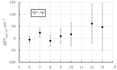
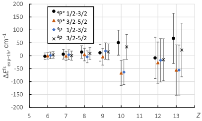
Fig. 4: Comparison of experimental and theoretical energies of the 1s(²S)2s2p(³P^∘) ⁴P^∘ and 1s2p^{2 4}P fine-structure energy levels of Li-like ions. Left: separations between centers of gravity of the quartet terms; right: fine-structure intervals within the quartet terms. Experimental data are from beam-foil experiments (see text). Theoretical data are from Yerokhin et al. [5]. The error bars are combinations in quadrature of the experimental and theoretical uncertainties. They are dominated by theoretical uncertainties.

As seen from Figure 4, the theoretical data of Yerokhin et al. [5] are entirely corroborated by this comparison: both the separations between the quartet terms and the fine-structure intervals within the terms agree with experiments. The uncertainties of all quantities compares in Figure 4 are dominated by the theoretical uncertainties specified by Yerokhin et al., and this comparison essentially validates these uncertainty estimates. For the separations between the quartet terms, the beam-foil experimental data are more precise than the theory [5] by a factor ranging between 2.5 and 7 (4.1 on average). For the fine-stricture intervals, these ratios are between 1.4 and 5.5 (2.9 on average). On the other hand, the connection between the quartet and doublet systems cannot be tested by these experimental data. Such tests are provided by the comparisons of absolute energy-level measurements described in the next subsection. They also confirm the validity of the data of Yerokhin et al. [5]. However, experimental precision of these absolute measurements is much lower than that of the theory (by a factor ranging from 18 to 250). Therefore, we chose the theoretical values of Yerokhin et al. [5] for the 1s(²S)2s2p(³P^∘) ⁴P${}^{\circ}_{3/2}$ base level (1o1) in each spectrum, which is used to determine the excitation energies from the ground level.

The experimental and theoretical data for the quartet levels discussed above are presented in Table LABEL:table:quart_E, where for each level we give the nuclear charge number of the atom, $Z$, the calculated energy and its uncertainty, $E_{\text{th}}$ and $u_{\text{th}}$, respectively, (in cm^-1) as given by Yerokhin et al. [5], recommended experimental energy $E_{\text{exp}}$ and its uncertainty $u_{\text{rel}}$ (in cm^-1) for separation from the 1s(²S)2s2p(³P^∘) ⁴P${}^{\circ}_{3/2}$ base level (1o1), and the list of references to the sources used to derive the level value. To determine the total uncertainty of the recommended energy for excitation from the ground level, the given $u_{\text{rel}}$ value must be combined in quadrature with the uncertainty $u_{\text{th}}$ of the theoretical energy of the base level. The contribution of the latter dominates in those total uncertainties.

5.2 Comparison of absolute energy measurements with theory

Absolute measurements of excitation energies are compared with theoretical calculations of Yerokhin et al. [5, 6] in Table LABEL:table:2. This table contains 999 measurements for $Z$ from 6 to 80. The table is divided into 16 sections with each section containing measurements of the same energy level in various spectra. The sections are sorted in the order of increasing excitation energy in C IV. The level identifiers are given at the top of each section. They start with the (2$J$)^π# identifier defined in Table A and are followed by the $LS$- and $jj$-coupling labels. As discussed in Section 2, the $LS$-coupling labels are valid for $Z\leq 38$, while the $jj$-labels should be used for greater $Z$. As mentioned in Section 2, the $jj$-labels of levels 3e1 and 3e2 for $Z\leq 53$ represent the second leading $jj$-component of their eigenvectors (see Table LABEL:table:composition_jj).

Each section of Table LABEL:table:2 contains the same set of columns. The first column is the nuclear charge of the element, $Z$. The second column is the sequential number $N_{m}$ of the measurement for the same level and the same $Z$. Sorting of these measurements is arbitrary. The only purpose of $N_{m}$ is to visualize the groups of measurements of the same quantity. The total number of distinct measured quantities (energy levels of a certain ion) is 329. Since there are 999 measurements in total, the average number of measurements per quantity is about three. The largest number of measurements, fifteen, is for the levels 1o2 and 3o2 (1s(²S)2s2p(³P^∘) ²P${}^{\circ}_{1/2,3/2}$) in O VI. Fourteen distinct energy levels in $Z$ = 6, 8, 10, 18, and 26 have ten or more measurements included in the table. For 137 quantities (about 42 % of the total 329), there is only one measurement available.

The third and fourth columns in Table LABEL:table:2 give the theoretical energy and its uncertainty ($E_{\text{th}}$ and $u_{\text{th}}$), both quoted from Yerokhin et al. [5] for $Z\leq 17$ and from Yerokhin and Surzhykov [6] for higher $Z$. The fifth and sixth columns give the experimentally measured energy and its uncertainty, respectively ($E_{\text{exp}}$ and $u_{\text{exp}}$). The reference to the original measurement is given in the last column of the table. We remind the reader that most of these measurements have been adjusted or corrected as described in Section 3, while some are our new determinations based on the data or figures of the original papers. Even in the cases where no changes were made to the originally reported data, we have evaluated and validated these original data and their uncertainties. Therefore, when quoting the data from our Table LABEL:table:2, it would be prudent to include a reference to the present paper.

The seventh column of Table LABEL:table:2 gives the value of the ‘dark uncertainty’, assigned to each measurement by our statistical analysis procedure described in Section 4. Out of 862 measurements that are not unique for the measured quantity (an energy level in a certain ion), only sixteen got assigned a non-zero dark uncertainty. Five of these dark uncertainty values are relatively small ($\leq 60$ % of the measurement uncertainty). They correspond to the cases of only a relatively small disagreement between the two or more measurements of the same quantity. The remaining cases represent a large disagreement between different studies and will be discussed further below.

The total experimental uncertainty, $u_{\text{etot}}$, given in the eighth column of Table LABEL:table:2 is the sum in quadrature of $u_{\text{exp}}$ and $u_{\text{dark}}$. It was used to determine the weighted mean experimental energy, $E_{\text{em}}$, and its uncertainty, $u_{\text{em}}$, given in the ninth and tenth columns, respectively. This derivation was made with the standard statistical formulas, $E_{\text{em}}$ = $(\Sigma E_{\text{exp}}u_{\text{etot}}^{-2})/\Sigma u_{\text{etot}}^{-2}$ and $u_{\text{em}}$ = $(\Sigma u_{\text{etot}}^{-2})^{-1/2}$. To make comparisons easier, the same values of $E_{\text{em}}$ and $u_{\text{em}}$ are repeated for all measurements of the same quantity.

The eleventh column of Table LABEL:table:2 contains the ratios of the uncertainties of the mean experimental and theoretical values, $u_{\text{em}}/u_{\text{th}}$. These ratios are given only in the rows containing the first measurement of a quantity ($N_{\text{m}}=1$). Only seven of these ratios are smaller than 1.0 (ranging from 0.14 to 0.77). They represent the cases where the mean experimental energy $E_{\text{em}}$ is more precise than the theoretical energy $E_{\text{em}}$. These few experimental results are all in good agreement with the theory (well within the combined uncertainties) and provide our recommended values for the level 1s(²S)2s2p(³P^∘) ⁴P${}^{\circ}_{5/2}$ (5o1) in S XIV, as well as the levels 1s(²S)2s2p(³P^∘) ²P${}^{\circ}_{1/2,3/2}$ (1o2 and 3o2) in S XIV, Cl XV, and Ar XVI. The next three columns of Table LABEL:table:2 contain three different normalized residuals: $R_{\text{e}-\text{em}}$, $R_{\text{em}-\text{t}}$, and $R_{\text{e}-\text{t}}$. All three represent the ratios of energy differences divided by the uncertainty of that difference. The first normalized residual, $R_{\text{e}-\text{em}}$, is for the differences between individual measurements of a quantity ($E_{\text{exp}}$) and its weighted experimental mean ($E_{\text{em}}$). These are non-blank only for the measurements that are not unique for the quantity measured and are used in the discussion of statistics of measurements. The second normalized residual, $R_{\text{em}-\text{t}}$, is used for comparing the mean experimental energy with theory. It is non-blank only in the rows with $N_{\text{m}}=1$. The third residual, $R_{\text{e}-\text{em}}$, is given for each measurement as a measure of deviation of this measurement from theory.

The last column of Table LABEL:table:2 gives the reference to each original measurement. Some of the original studies contained two or more measurements of the same spectrum. If these measurements were made with a similar technique, we derived a mean value that is given in Table LABEL:table:2. However, the results presented by Matthews et al. [70] were obtained with two very different techniques, X-ray emission and Auger electron spectroscopy. We treat these results as independent measurements. Thus, the reference [70] is followed by ‘(Auger)’ or ‘(X-ray)’ in Table LABEL:table:2 to distinguish between these two sets of results.

For rounding of values given with uncertainties in Table LABEL:table:2, the “rule-of-99” based on the uncertainty value was used. Literally, the rule is formulated as follows: in units of the last significant digit of the value, the uncertainty must be not greater than 99 and not smaller than 10, always keeping two significant digits in the uncertainty. This preserves a reasonable numerical precision of the values in line with recommendations of International Committee for Weights and Measures (CIPM; formerly BIPM), see Ref. [147], Section 7.2.6.

In the table, the fractional number of measurements with $R_{\text{e}-\text{t}}\leq 1.0$ and $R_{\text{e}-\text{t}}\leq 2.0$ are 90.6 % and 99.7 %, respectively. For the ratio $R_{\text{em}-\text{t}}$, the corresponding fractions are 84.5 % and 99.1 %, respectively.

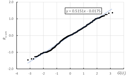
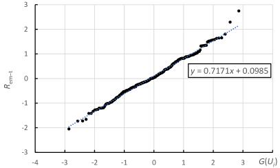
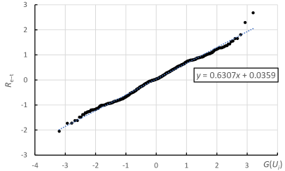
Fig. 5: Normal probability plots of three normalized residuals given in Table LABEL:table:2: $R_{\text{e}-\text{em}}$ (top left), $R_{\text{em}-\text{t}}$ (top right), and $R_{\text{e}-\text{t}}$ (bottom). The quantity $G(U_{i})$ on the horizontal axes of these plots is the percent point function of the uniform order statistic median of the normal distribution [146]. The dotted lines are linear fits to the data points.

Normal probability plots of the three normalized residuals are shown in Fig. 5. For detailed explanations of properties of such plots, see Filliben and Heckert [146]. Briefly, the residual values $R_{i}$ are sorted in increasing order and numbered sequentially with their index $i$. Then they are plotted against the values of the function $G(U_{i})$, which is the percent point function of the uniform order statistic median of the normal distribution. If the statistical distribution function of the measurements is close to normal, the points on the plot lie close to a straight line with a slope of 1.0 crossing the origin. All three plots in Fig. 5 are indeed close to a straight line crossing the origin, but the slopes are significantly less than 1.0. This may indicate that the total uncertainties of the energy differences used in the calculation of these normalized residuals are overestimated by a factor between 1.5 and 2. Those uncertainties are in most cases dominated by the measurement uncertainties. Their overestimation may be due to a significant contribution of systematic uncertainties. The plot of $R_{\text{e}-\text{em}}$ (Fig. 5, top left) shows that the measurements themselves are internally consistent, i.e., there are no abnormally large discrepancies between individual measurements and their weighted means. The plot of $R_{\text{em}-\text{t}}$ (Fig. 5, top right) shows that the mean experimental energies are all statistically consistent with theory, although the two points in the right upper corner of the plot visibly deviate from the overall linear trend. These two points correspond to the level 1s(²S)2s2p(³P^∘) ⁴P${}^{\circ}_{5/2}$ (5o1) in Ar XVI and 1s(²S)2s2p(³P^∘) ²P${}^{\circ}_{3/2}$ (3o2) in Co XXV. They will be discussed further below.

The third normal probability plot (Fig. 5, bottom) shows the distribution of differences of all individual measurements from theory. One can see that there are no individual measurements with abnormally large differences from theory. The two points in the right upper corner of this plot correspond to the same levels (5o1 in Ar XVI and 3o2 in Co XXV) that are somewhat off the linear trend of $R_{\text{em}-\text{t}}$ discussed above. These are the measurements of Machado et al. [64] for Ar XIV and Smith et al. [93] for Co XXV. Although the deviations of these measurements from theory are entirely within the statistically allowed range for a set of nearly a thousand measurements, it is worth discussing their possible reasons.

The 5o1 level of Ar XVI is directly measured by Machado et al. [64] as the energy of the U satellite line (see Table B for the definition of satellite line labels). Figure 6 of their paper indicates that this measurement might have been affected (shifted to higher energies) by presence of a small additional peak on the wing of the stronger high-energy peak. Such a small peak was indeed detected and measured by Machado et al. in the spectrum of S XIV (see their Fig. 9 and its discussion in [64]). This peak corresponds to the satellite transition i. However, Machado et al. stated that they could not find statistical evidence for the presence of this peak in the argon spectrum. Figure 6(b) of Ref. [64] gives a hint that this might have been due to a combination of a too low signal-to-noise ratio and an imperfection of the modeled shape of the much stronger peak at a higher energy (which is due to Be-like Ar).

The 3o2 level in Co XXV is defined by the wavelength of the satellite line q reported by Smith et al. [93] to be at 1.72126(11) Å. According to the calculations presented in Table I of their paper, this line should have been at least 10 times weaker than the satellite ‘a’ located very close to it at the longer-wavelength side. On the short-wavelength side, also within the line width, there is the strong He-like intercombination line y. Figure 3 of Smith et al. indicates that, even if the blending problems might have been mitigated by the use of different beam energies, the signal-to-noise ratio must have been very low for the weak q line, so the small uncertainty assigned to its wavelength was probably underestimated.

Let us now turn to the discussion of measurements that were penalized by large dark uncertainty values in our statistical analysis (see Section 4).

As mentioned in Section 3, the measurement of the q+r satellite line in O VI by Liao et al. [128] was found to strongly deviate from the other 14 measurements available for this line. This measurement is responsible for experimental values of two energy levels included in Table LABEL:table:2: 1s(²S)2s2p(³P^∘) ²P^∘ $J$ = 1/2 (1o2) and $J$ = 3/2 (3o2) at $Z=8$. Both statistical models of Rukhin [144, 145], CMLE and CRMLE, unanimously singled out this measurement and assigned to it a large dark uncertainty value of about 1500 cm^-1, which resulted in the total uncertainty $u_{\text{etot}}=1600$ cm^-1. This is more than three times greater than the uncertainty specified by Liao et al., 470 cm^-1. It corresponds to the wavelength uncertainty of 0.008 Å, while Liao et al. stated it to be $(^{+0.0023}_{-0.0020})$ Å. The line in question is marked as O VI K$\alpha$ in Fig. 3 of Liao et al. (bottom panel) near 22 Å. From this figure, the full width at half maximum is about 0.032 Å for this line. It is unlikely that an error of 0.008 Å could be due to statistical uncertainties of fitting the line profile. There must have been either an error in the calibration of the wavelength scale or some physical phenomenon peculiar to absorption spectra of the interstellar media studied by Liao et al. We note that the wavelength of this line measured by Yao et al. [105] and by Gatuzz et al. [47] in similar absorption spectra of interstellar media is also too long compared to the laboratory measurements, as well as the calculations of Yerokhin et al. [5], which suggests that a physical explanation (unknown at present) is more likely than a calibration error. The measurements of Yao et al. and Gatuzz et al. had larger uncertainties (0.004 Å and 0.003 Å, respectively) and thus are statistically compatible with the laboratory measurements. The large dark uncertainty assigned to the measurement of Liao et al. makes its contribution to the determination of the experimental mean very small and masks the problem in comparison plots. However, we stress that this is an unresolved problem requiring additional experimental and theoretical study.

Another important case is the measurement of the same q and r satellite transitions in S XIV by Machado et al. [64]. Unlike the oxygen measurements discussed above, these satellite transitions were well resolved in the sulfur spectra observed by Machado et al. Both the CMLE and CRMLE methods assigned relatively large dark uncertainties to these measurements, 390 cm^-1 for the 1o2 level (r line) and 440 cm^-1 for the 3o2 level (q line), to be compared with the reported uncertainties of 89 cm^-1 and 81 cm^-1, respectively [64]. For each of these two levels, there are six measurements included in Table LABEL:table:2. However, only three of them have uncertainties small enough to influence the experimental means. These are the measurements of Machado et al. [64], Schlesser et al. [88], and Hell et al. [53]. Although in the latter work the q and r lines were unresolved, we extracted the separate values for their upper levels, 3o2 and 1o2, by using their theoretical separation [5]. The resulting values agree very well with those reported by Schlesser et al., which leads to singling out the measurements of Machado et al. as discrepant. For these two O VI levels, the uncertainties of experimental mean energies are a few times smaller than those of the theoretical data [5]. Thus, these values are included in the list of the few experimental values that we recommend as reference data. Nevertheless, the discrepancy discussed above calls for an additional experimental study.

All other cases of a non-zero dark uncertainty involve relatively low-resolution measurements in laser-produced, vacuum-spark, tokamak, or EBIT plasmas in $Z=10$ [80, 103], $Z=21$ [25, 81, 99], $Z=24$ [99], $Z=26$ [36], and $Z=28$ [86, 26]. For each of the levels involved, there are only two or three measurements available, and their uncertainties are comparable. The additional dark uncertainties assigned to these measurements range from 0.02 to 1.6 of the $u_{\text{exp}}$ values of Table LABEL:table:2. They may be explained by difficulties in interpretation of partially blended line profiles in these experiments.

In addition to the normal probability plots shown in Fig. 5, it would be interesting to see a direct comparison of the experimental and theoretical values similar to the plots presented in the review of H- and He-like spectra by Indelicato [117]. This turned out difficult because of the large number of measurements (999) and the wide range of their precision (between 1 part in 10⁶ and 6 parts in 10³). To make plots easier to view, we scaled the measured energies by $Z^{-2}$ and divided all measurements into four sets based on their scaled uncertainties. Instead of making plots for each energy level, we chose to plot data for all levels together. These plots are presented in Fig. 6.

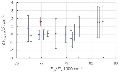
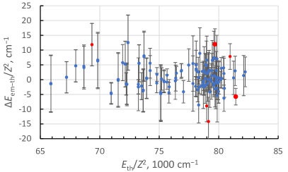
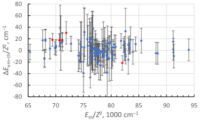
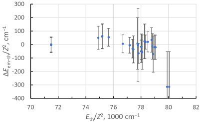
Fig. 6: Differences between scaled experimental and theoretical core-excited $n=2$ energy levels of Li-like ions. Experimental values are the mean values ($E_{\text{em}}$) given in Table LABEL:table:2. Theoretical data are from Yerokhin et al. [5] for $Z\leq 17$ and from Yerokhin and Surzhykov [6] for higher $Z$. The small red dots correspond to the cases of a moderate disagreement ($1<|R_{\text{em}-\text{t}}|<1.5$ in Table LABEL:table:2). The large red circles indicate a large disagreement ($|R_{\text{em}-\text{t}}|>1.5$).

The most meaningful comparison of theory with experiment is given by the top left panel of Fig. 6, which contains the energy differences ${\Delta}E_{\text{em}-\text{th}}$ with the smallest scaled uncertainties, $u_{\text{sc}}=(u_{\text{exp}}^{2}+u_{\text{th}}^{2})^{1/2}/Z^{2}<2$ cm^-1. This panel contains measurements in $Z=14,16,17,18,26$, and 36. The ratios of the experimental and theoretical uncertainties, $u_{\text{em}}/u_{\text{th}}$, range between 0.14 and 5.3 for these measurements (see Table LABEL:table:2). In this panel, the only point showing a large discrepancy between experiment and theory corresponds to the measurements of the U transition in Ar XVI. The mean experimental value for the upper level of this transition, 5o1, is dominated by the high-precision measurement of Machado et al. [64]. The possible reasons of its discrepancy with theory have already been discussed above.

The top right panel of Fig. 6 represents less precise comparisons with the total uncertainties $u_{\text{sc}}$ in the range between 2 cm^-1 and 10 cm^-1. One can see that there are only two strongly discrepant data points in this panel. One of them corresponds to the measurement of the q satellite in $Z=27$ by Smith et al. [93], which was already discussed above. The other one is for the 1s(²S)2s2p(¹P^∘) ²P${}^{\circ}_{3/2}$ (3o3) level in Kr XXXIV ($Z=36$) by Widmann et al. [104]. This level is defined by the measured wavelength of the ‘s’ satellite, 0.94761(3) Å. As explained in Section 3, similar to several other studies published by the LLNL group, we adjusted the wavelength calibration of Widmann et al. by subtracting the weighted average difference of the reported He-like lines w, x, y, and z from the precise reference values of Artemyev et al. [114]. This correction amounted to $-0.000007(11)$ Å and decreased the s-satellite wavelength to 0.94760(3) Å. This is the value we used to derive the experimental energy of the 3o3 level in Table LABEL:table:2. It is the only measurement available for this level in Kr XXXIV. Although the correction decreased the discrepancy with Yerokhin and Surzhykov [6] from $-2.5\sigma$ to $-2.1\sigma$, it is still significant and calls for additional experimental studies. We note that the theoretical uncertainty for this level [6] is seven times smaller than that of Widmann et al., so it is unlikely that the reason for the discrepancy is related to theory. It might be due to blending with some other line, e.g., from a $n=3$ Li-like satellite transition, which was not suspected in the study of Widmann et al.

The bottom panels of Fig. 6 show the scaled energy differences between experiment and theory for the much cruder measurements with scaled uncertainties $u_{\text{sc}}$ in the ranges (10–50) cm^-1 (left bottom) and (50–270) cm^-1 (right bottom).

Overall, the comparisons shown in Fig. 6 show a good agreement of experiments with theory. There are only a few measurements that deviate from theory by more than 1.5$\sigma$ (the red circles in the plots), and they are all well within the range of deviations that can be expected for a normal statistical distribution. This corroborates the conclusion following from the normal probability plots shown in Fig. 5: the theory of Yerokhin et al. [5, 6] largely agrees with the available experimental data. Thus, we recommend the use of these theoretical data in the cases where more precise experimental data are not available.

However, we must note that the theory [5, 6] is really contested by absolute energy measurement only for $Z=16$, 17, and 18, where the ratios of experimental and theoretical uncertainties, $u_{\text{em}}/u_{\text{th}}$, are smaller than $\approx 1.5$ (see Table LABEL:table:2). For measurements of the energy intervals within the quartet system, this theory is contested (and confirmed) by experiments for $Z=6$–13 (see subsection 5.1. Therefore, high-precision measurements are still needed to meaningfully test the theory for heavier elements ($Z>18$), and our recommendation for these elements can only be treated as provisional.

6 Conclusion

For the 16 energy levels of the 1s2$l$2$l^{\prime}$ core-excited configurations of Li-like ions, 999 absolute and 35 relative experimental energy-level measurements from 101 publications have been collected and analyzed. Except for a small number of measurements discussed in the previous Sections, agreement between the experimental and theoretical data is very good: all the data obey the normal statistical distribution for the combined (experimental and theoretical) uncertainties. For 35 energy intervals of quartet levels relative to the second lowest quartet level, we provide recommended values derived from experimental data. We also provide recommended absolute experimental energies for seven levels: 1s(²S)2s2p(³P^∘) ⁴P${}^{\circ}_{5/2}$ (5o1) in S XIV, as well as the levels 1s(²S)2s2p(³P^∘) ²P${}^{\circ}_{1/2,3/2}$ (1o2 and 3o2) in S XIV, Cl XV, and Ar XVI. For the rest of the 1s2$l$2$l^{\prime}$ levels in all Li-like spectra of the elements between carbon and uranium, we recommend the use of the theoretical data of Yerokhin et al. [5, 6] for modeling plasma spectra and for calibration of experimental X-ray spectral measurements in ions with a larger number of electrons. The validity of these theoretical data is meaningfully tested and confirmed for nuclear charges $Z\leq 18$. For higher $Z$, although all available measurements also agree with this theory, their precision is insufficient for a meaningful comparison. High-precision measurements are still needed to contest the theory in this high-$Z$ region.

Several problems in interpretation of experimental data have been detected. Some of them have been solved by re-calibration of experimental wavelength scale and correcting the identification of observed spectral features. However, a few cases require additional experimental and/or theoretical work. One example is the absorption spectrum of Li-like oxygen observed in interstellar media studied with the Chandra orbital X-ray laboratory [105, 47, 128]. Another example is the absorption spectrum measurements using synchrotrons [85, 126, 71]. Such experiments can potentially reach very high precision, but this requires an improvement in the instrumentation used.

A new framework of statistical treatment of experimental data has been developed and successfully tested in this work. The newly designed statistics module for Excel implements the recently developed statistical methods for estimation of hidden errors in experiments by using the clustered maximum likelihood and restricted maximum likelihood estimators. This implementation was found to work efficiently in comparisons of up to 22 independent measurements of a single quantity. For a greater number of measurements, the number of possible combinations that needs to be tested to find the optimal division of the data pool into clusters becomes too large to be tractable by these methods. More research is needed to further develop methods for statistical treatment of large sets of measurements.

Explanation of Tables

Table LABEL:table:quart_E. Recommended theoretical and experimental energies of core-excited 1s2$l$2$l^{\prime}$ quartet levels in Li-like ions.
Experimental energies are derived from beam-foil measurements of separations of levels relative to the 1s2s2p ⁴P${}^{\circ}_{3/2}$ level.

$Z$	Atomic number
Lbl	Level label in Table A
Configuration	Configuration label in $LS$ coupling
Term	Term label in $LS$ coupling
$J$	Total angular momentum quantum number
$E_{\text{th}}$	Calculated energy (cm-1) [5]
$u_{\text{th}}$	Uncertainty of the calculated energy (cm-1) [5]
$E_{\text{exp}}$	Experimental energy (cm-1)
$u_{\text{rel}}$	Uncertainty of the experimental separation from the 1s2s2p 4P${}^{\circ}_{3/2}$ base level (cm-1).
	To obtain the total uncertainty of excitation energy from the ground level, add $u_{\text{th}}$ of the
	base level in quadrature.
References	Reference to studies used to derive the level value. TW means ‘This Work’.

Table LABEL:table:quart_wl. Experimental and recommended (Ritz) wavenumbers for transitions between core-excited 1s2$l$2$l^{\prime}$ quartet levels in Li-like ions.
Observed wavelengths and wavenumbers are derived as weighted means of beam-foil measurements.
Recommended Ritz wavenumbers are derived in a least-squares level optimization in this work.

$Z$	Atomic number
Lbl1	Lower level label in Table A
Lbl2	Upper level label in Table A
$\lambda_{\text{obs}}$	Observed wavelength in Å
$u(\lambda_{\text{obs}})$	Uncertainty of observed wavelength in Å
$\sigma_{\text{obs}}$	Observed wavenumber in cm-1
$u(\sigma_{\text{obs}})$	Uncertainty of observed wavenumber in cm-1
$\sigma_{\text{Ritz}}$	Ritz wavenumber in cm-1. This is the recommended experimental value derived in this
	work.
$u(\sigma_{\text{Ritz}})$	Uncertainty of Ritz wavenumber in cm-1
$E_{1}$	Lower level value in cm-1 from Table LABEL:table:quart_E
$E_{2}$	Upper level value in cm-1 from Table LABEL:table:quart_E
F	Line flag: P – predicted wavenumber; b – blended line
Weight	Transition weight in the level optimization procedure (1 for unblended lines, 0 for lines
	excluded from the level optimization, other values for blended lines)
References	References to line observations used to derive the weighted mean $\lambda_{\text{obs}}$

Table LABEL:table:2. Comparison of theoretical and experimental energies of the core-excited 1s2$l$2$l^{\prime}$ states in Li-like ions.

$Z$	Atomic number
$E_{\text{th}}$	Calculated energy (cm-1) [5, 6]
$U_{\text{th}}$	Uncertainty of the calculated energy (cm-1) [5, 6]
$E_{\text{exp}}$	Experimental energy (cm-1)
$U_{\text{exp}}$	Uncertainty of the experimental energy (cm-1)
${\Delta}$	Difference between the experimental and calculated energy values,
	$E_{\text{exp}}-E_{\text{th}}$ (cm-1)
$R$	Ratio ${\Delta}$/$U_{\text{exp}}$ of the difference between the experimental
	and calculated energy values to the uncertainty of the experimental energy
$E_{\text{exp,mean}}$	Mean experimental energy (cm-1), averaged over all values $E_{\text{exp}}$
	with the same $Z$ using weights equal to $U_{\text{exp}}^{-2}$
$U_{\text{exp,mean}}$	Uncertainty of the mean experimental energy (cm-1)
${\Delta}_{\text{mean}}$	Difference between the mean experimental and calculated energy values,
	$E_{\text{exp,mean}}-E_{\text{th}}$ (cm-1)
$U_{\text{mean}}$	Uncertainty of the difference between the mean experimental and
	calculated energy values (cm-1), with $U_{\text{th}}$ included
$R_{\text{mean}}$	Ratio ${\Delta}_{\text{mean}}$/$U_{\text{mean}}$ of the difference between the mean experimental
	and calculated energy values to the uncertainty of the difference
$N$	The number of the data point (measurement number) for the given level
Ref	Reference

Table 1: Recommended theoretical and experimental energies of core-excited 1s2$l$2$l^{\prime}$ quartet levels in Li-like ions. Experimental energies are derived from beam-foil measurements of separations of levels relative to the 1s2s2p ⁴P${}^{\circ}_{3/2}$ level. See page Table . Recommended theoretical and experimental energies of core-excited 1s2$l$2$l^{\prime}$ quartet levels in Li-like ions. Experimental energies are derived from beam-foil measurements of separations of levels relative to the 1s2s2p ⁴P${}^{\circ}_{3/2}$ level. for Explanation of Tables.

$Z$	Lbl	Configuration	Term	$J$	$E_{\text{th}}$	$u_{\text{th}}$	$E_{\text{exp}}$	$u_{\text{rel}}$	References
					cm-1	cm-1	cm-1	cm-1
6	1o1	1s(2S)2s2p(3P∘)	4P∘	1/2	2371985	9	2371987.9	2.8	[109, 107, 5],TW
6	3o1	1s(2S)2s2p(3P∘)	4P∘	3/2	2371989	9	2371990.6	0.0	[109, 107, 5],TW
6	5o1	1s(2S)2s2p(3P∘)	4P∘	5/2	2372086	9	2372086.8	2.3	[109, 107, 5],TW
6	1e2	1s(2S)2p2(3P)	4P	1/2	2446336	9	2446332.3	2.1	[109, 107, 5],TW
6	3e1	1s(2S)2p2(3P)	4P	3/2	2446412	9	2446409.4	2.4	[109, 107, 5],TW
6	5e1	1s(2S)2p2(3P)	4P	5/2	2446451	9	2446452.3	1.8	[109, 107, 5],TW
7	1o1	1s(2S)2s2p(3P∘)	4P∘	1/2	3337990	11	3337980	8	[109, 5],TW
7	3o1	1s(2S)2s2p(3P∘)	4P∘	3/2	3338024	11	3338015	0	[109, 5],TW
7	5o1	1s(2S)2s2p(3P∘)	4P∘	5/2	3338236	11	3338227	7	[109, 5],TW
7	1e2	1s(2S)2p2(3P)	4P	1/2	3427951	11	3427956	7	[109, 5],TW
7	3e1	1s(2S)2p2(3P)	4P	3/2	3428109	11	3428122	6	[109, 5],TW
7	5e1	1s(2S)2p2(3P)	4P	5/2	3428222	11	3428233	6	[109, 5],TW
8	1o1	1s(2S)2s2p(3P∘)	4P∘	1/2	4468990	15	4468986	10	[109, 5],TW
8	3o1	1s(2S)2s2p(3P∘)	4P∘	3/2	4469088	15	4469094	0	[109, 5],TW
8	5o1	1s(2S)2s2p(3P∘)	4P∘	5/2	4469497	15	4469506	10	[109, 5],TW
8	1e2	1s(2S)2p2(3P)	4P	1/2	4574629	14	4574627	8	[109, 5],TW
8	3e1	1s(2S)2p2(3P)	4P	3/2	4574924	14	4574917	8	[109, 5],TW
8	5e1	1s(2S)2p2(3P)	4P	5/2	4575172	14	4575172	9	[109, 5],TW
9	1o1	1s(2S)2s2p(3P∘)	4P∘	1/2	5765148	21	5765143	11	[111, 5],TW
9	3o1	1s(2S)2s2p(3P∘)	4P∘	3/2	5765357	21	5765358	0	[111, 5],TW
9	5o1	1s(2S)2s2p(3P∘)	4P∘	5/2	5766077	21	5766072	11	[111, 5],TW
9	1e2	1s(2S)2p2(3P)	4P	1/2	5886600	20	5886591	14	[111, 5],TW
9	3e1	1s(2S)2p2(3P)	4P	3/2	5887104	20	5887107	8	[111, 5],TW
9	5e1	1s(2S)2p2(3P)	4P	5/2	5887577	20	5887591	8	[111, 5],TW
10	1o1	1s(2S)2s2p(3P∘)	4P∘	1/2	7226607	33	7226590	12	[108, 110, 5],TW
10	3o1	1s(2S)2s2p(3P∘)	4P∘	3/2	7226994	33	7227021	0	[108, 110, 5],TW
10	5o1	1s(2S)2s2p(3P∘)	4P∘	5/2	7228173	33	7228141	12	[108, 110, 5],TW
10	1e2	1s(2S)2p2(3P)	4P	1/2	7364053	33	7364088	9	[108, 110, 5],TW
10	3e1	1s(2S)2p2(3P)	4P	3/2	7364867	33	7364847	9	[108, 110, 5],TW
10	5e1	1s(2S)2p2(3P)	4P	5/2	7365686	33	7365694	9	[108, 110, 5],TW
12	1o1	1s(2S)2s2p(3P∘)	4P∘	1/2	10646364	55	10646349	19	[112, 5],TW
12	3o1	1s(2S)2s2p(3P∘)	4P∘	3/2	10647382	55	10647360	0	[112, 5],TW
12	5o1	1s(2S)2s2p(3P∘)	4P∘	5/2	10650117	55	10650071	18	[112, 5],TW
12	1e2	1s(2S)2p2(3P)	4P	1/2	10816615	55	10816652	29	[112, 5],TW
12	3e1	1s(2S)2p2(3P)	4P	3/2	10818457	55	10818489	13	[112, 5],TW
12	5e1	1s(2S)2p2(3P)	4P	5/2	10820468	55	10820483	20	[112, 5],TW
13	1o1	1s(2S)2s2p(3P∘)	4P∘	1/2	12605132	66	12605086	27	[113, 106, 5],TW
13	3o1	1s(2S)2s2p(3P∘)	4P∘	3/2	12606652	66	12606662	0	[113, 106, 5],TW
13	5o1	1s(2S)2s2p(3P∘)	4P∘	5/2	12610590	66	12610554	27	[113, 106, 5],TW
13	1e2	1s(2S)2p2(3P)	4P	1/2	12792324	66	12792375	13	[113, 106, 5],TW
13	3e1	1s(2S)2p2(3P)	4P	3/2	12794956	66	12794961	23	[113, 106, 5],TW
13	5e1	1s(2S)2p2(3P)	4P	5/2	12797892	66	12797909	39	[113, 106, 5],TW

Table 1: (continued)

Table 2: Experimental and recommended (Ritz) wavenumbers for transitions between core-excited 1s2$l$2$l^{\prime}$ quartet levels in Li-like ions. Observed wavelengths and wavenumbers are derived as weighted means of beam-foil measurements. Recommended Ritz wavenumbers are derived in a least-squares level optimization in this work. See page Table . Experimental and recommended (Ritz) wavenumbers for transitions between core-excited 1s2$l$2$l^{\prime}$ quartet levels in Li-like ions. Observed wavelengths and wavenumbers are derived as weighted means of beam-foil measurements. Recommended Ritz wavenumbers are derived in a least-squares level optimization in this work. for Explanation of Tables.

$Z$	Lbl1	Lbl2	$\lambda_{\text{obs}}$	$u(\lambda_{\text{obs}})$	$\sigma_{\text{obs}}$	$u(\sigma_{\text{obs}})$	$\sigma_{\text{Ritz}}$	$u(\sigma_{\text{Ritz}})$	$\Delta\sigma_{\text{obs}-\text{Ritz}}$	$E_{1}$	$E_{2}$	F	Weight	References
			Å	Å	cm-1	cm-1	cm-1	cm-1	cm-1	cm-1	cm-1
6	3o1	5e1	1342.990	0.037	74460.7	2.1	74461.7	1.8	$-1$	2371990.6	2446452.3		1	[109, 107]
6	1o1	3e1	1343.690	0.037	74421.9	2.3	74421.5	2.1	$0.4$	2371987.9	2446409.4		0.781	[109, 107]
6	3o1	3e1	1343.690	0.037	74421.9	4.4	74418.8	2.4	$3.1$	2371990.6	2446409.4		0.219	[109, 107]
6	5o1	5e1	1344.690	0.037	74366.6	2.0	74365.5	1.8	$1.1$	2372086.8	2446452.3		1	[109, 107]
6	1o1	1e2	1345.133	0.037	74342.1	4.4	74344.4	3.0	$-2.3$	2371987.9	2446332.3		0.214	[109, 107]
6	3o1	1e2	1345.133	0.037	74342.1	2.3	74341.7	2.1	$0.4$	2371990.6	2446332.3		0.786	[109, 107]
6	5o1	3e1	1345.507	0.037	74321.4	2.0	74322.6	1.8	$-1.2$	2372086.8	2446409.4		1	[109, 107]
6	1e2	3e1					77.1	2.8		2446332.3	2446409.4	P	0
6	3e1	5e1					42.9	2.3		2446409.4	2446452.3	P	0
7	3o1	5e1	1108.4	0.1	90220	8	90218	6	$2$	3338015	3428233		1	[109]
7	1o1	3e1	1109.3	0.1	90147	8	90141	7	$6$	3337980	3428122		1	[109]
7	3o1	3e1	1109.8	0.1	90106	8	90107	6	$0$	3338015	3428122		1	[109]
7	5o1	5e1	1111.0	0.1	90009	8	90006	6	$4$	3338227	3428233		1	[109]
7	1o1	1e2					89976	10		3337980	3427956	P	0
7	3o1	1e2	1111.8	0.1	89944	8	89941	7	$3$	3338015	3427956		1	[109]
7	5o1	3e1	1112.4	0.1	89896	8	89894	6	$1$	3338227	3428122		1	[109]
7	1e2	3e1					165	8		3427956	3428122	P	0
7	3e1	5e1					111	7		3428122	3428233	P	0
8	3o1	5e1	942.7	0.1	106078	11	106077	9	$1$	4469094	4575172		1	[109]
8	1o1	3e1	944.0	0.1	105932	11	105931	9	$1$	4468986	4574917		1	[109]
8	3o1	3e1	945.0	0.1	105820	11	105823	8	$-2$	4469094	4574917		1	[109]
8	5o1	5e1	946.4	0.1	105664	11	105665	9	$-2$	4469506	4575172		1	[109]
8	1o1	1e2	946.6	0.1	105641	11	105640	9	$1$	4468986	4574627		1	[109]
8	3o1	1e2	947.6	0.1	105530	11	105532	8	$-2$	4469094	4574627		1	[109]
8	5o1	3e1	948.7	0.1	105407	11	105411	9	$-3$	4469506	4574917		1	[109]
8	1e2	3e1					291	9		4574627	4574917	P	0
8	3e1	5e1					255	9		4574917	4575172	P	0
9	3o1	5e1	818.09	0.06	122235.9	9	122234	8	$2$	5765358	5887591		1	[111]
9	1o1	3e1	819.89	0.06	121967.6	9	121965	8	$3$	5765143	5887107		1	[111]
9	3o1	3e1	821.37	0.06	121747.8	9	121750	8	$-2$	5765358	5887107		1	[111]
9	5o1	5e1	822.91	0.06	121520	9	121519	8	$1$	5766072	5887591		1	[111]
9	1o1	1e2	823.42	0.08	121445	12	121448	11	$-4$	5765143	5886591		1	[111]
9	3o1	1e2			121214		121234	14		5765358	5886591	P	0
9	5o1	3e1			121032		121035	13		5766072	5887107	P	0
9	1e2	3e1					516	12		5886591	5887107	P	0
9	3e1	5e1					484	11		5887107	5887591	P	0
10	3o1	5e1	721.11	0.05	138675.1	9.6	138673	9	$2$	7227021	7365694		1	[108, 110]
10	1o1	3e1	723.29	0.05	138257.1	9.6	138256	9	$1$	7226590	7364847		1	[108, 110]
10	3o1	3e1	725.59	0.05	137818.9	9.5	137826	9	$-7$	7227021	7364847		1	[108, 110]
10	5o1	5e1	727.15	0.20	137523	53	137553	14	$-29$	7228141	7365694	b	0.73	[108, 110]
10	1o1	1e2	727.15	0.20	137523	53	137497	15	$26$	7226590	7364088	b	0.27	[108, 110]
10	3o1	1e2	729.56	0.05	137068.9	9.4	137067	9	$2$	7227021	7364088		1	[108, 110]
10	5o1	3e1	731.48	0.05	136709.1	9.3	136705	9	$4$	7228141	7364847		1	[108, 110]
10	1e2	3e1					759	12		7364088	7364847	P	0
10	3e1	5e1					847	12		7364847	7365694	P	0
12	3o1	5e1	577.62	0.08	173124	24	173123	20	$1$	10647360	10820483		1	[112]
12	1o1	3e1	580.93	0.05	172138	15	172140	14	$-2$	10646349	10818489		1	[112]
12	3o1	3e1	584.35	0.05	171130	15	171129	13	$1$	10647360	10818489		1	[112]
12	5o1	5e1	586.80	0.15	170416	44	170412	24	$4$	10650071	10820483		1	[112]
12	1o1	1e2	587.10	0.15	170329	44	170303	29	$26$	10646349	10816652		1	[112]
12	3o1	1e2	590.70	0.15	169291	43	169292	29	$-1$	10647360	10816652	b	1	[112]
12	5o1	3e1	593.75	0.05	168421	14	168418	13	$3$	10650071	10818489		1	[112]
12	1e2	3e1					1837	29		10816652	10818489	P	0
12	3e1	5e1					1994	22		10818489	10820483	P	0
13	3o1	5e1	522.95	0.17	191223	62	191247	39	$-24$	12606662	12797909	b	1	[113, 106]
13	1o1	3e1	526.67	0.05	189872	18	189875	17	$-3$	12605086	12794961		1	[113, 106]
13	3o1	3e1	531.04	0.08	188310	28	188299	23	$11$	12606662	12794961		1	[113, 106]
13	5o1	5e1	533.64	0.17	187392	60	187355	39	$37$	12610554	12797909	b	1	[113, 106]
13	1o1	1e2	533.73	0.17	187361	60	187289	28	$72$	12605086	12792375	b	1	[113, 106]
13	3o1	1e2	538.47	0.04	185711	14	185713	13	$-2$	12606662	12792375		1	[113, 106]
13	5o1	3e1	542.28	0.05	184407	17	184407	16	$0$	12610554	12794961		1	[113, 106]
13	1e2	3e1					2586	25		12792375	12794961	P	0
13	3e1	5e1					2948	39		12794961	12797909	P	0

Table 2: (continued)

Table 3: Comparison of theoretical and experimental energies of core-excited 1s2$l$2$l^{\prime}$ states in Li-like ions. See page Table . Comparison of theoretical and experimental energies of the core-excited 1s2$l$2$l^{\prime}$ states in Li-like ions. for Explanation of Tables

$Z$	$N_{\text{m}}$	$E_{\text{th}}$	$u_{\text{th}}$	$E_{\text{exp}}$	$u_{\text{exp}}$	$u_{\text{dark}}$	$u_{\text{etot}}$	$E_{\text{em}}$	$u_{\text{em}}$	$u_{\text{em}}/u_{\text{th}}$	$R_{\text{e}-\text{em}}$	$R_{\text{em}-\text{t}}$	$R_{\text{e}-\text{t}}$	Ref
		cm-1	cm-1	cm-1	cm-1	cm-1	cm-1	cm-1	cm-1
1e1: 1s2s2 2S1/2 or [1s2s2]1/2
6	1	2351890	66	2355900	4000	0	4000	2351790	480	7.3	1.03	-0.21	1.00	[83]
6	2	2351890	66	2355100	8100	0	8100	2351790	480		0.41		0.40	[90]
6	3	2351890	66	2351860	810	0	810	2351790	480		0.09		-0.04	[67]
6	4	2351890	66	2350200	4400	0	4400	2351790	480		-0.36		-0.38	[54]
6	5	2351890	66	2351710	860	0	860	2351790	480		-0.09		-0.21	[68]
6	6	2351890	66	2351460	990	0	1000	2351790	480		-0.33		-0.43	[65]
6	7	2351890	66	2352100	1700	0	1700	2351790	480		0.18		0.12	[62]
7	1	3314286	66	3318100	8300	0	8300	3315130	880	13	0.36	0.96	0.46	[54]
7	2	3314286	66	3315100	890	0	890	3315130	880		-0.04		0.91	[65]
8	1	4441684	66	4442700	1600	0	1600	4442850	710	11	-0.09	1.63	0.63	[28]
8	2	4441684	66	4447000	12000	0	12000	4442850	710		0.35		0.44	[54]
8	3	4441684	66	4441300	3800	0	3800	4442850	710		-0.41		-0.10	[52]
8	4	4441684	66	4443060	900	0	900	4442850	710		0.23		1.53	[65]
8	5	4441684	66	4442400	1900	0	1900	4442850	710		-0.24		0.38	[62]
9	1	5734301	66	5737800	8300	0	8300	5737500	3100	48	0.04	1.00	0.42	[54]
9	2	5734301	66	5737400	3400	0	3400	5737500	3100		-0.02		0.91	[61]
10	1	7192195	77	7188900	4100	0	4100	7192770	610	7.9	-0.94	0.94	-0.80	[94]
10	2	7192195	77	7192830	810	0	810	7192770	610		0.07		0.78	[29]
10	3	7192195	77	7196000	13000	0	13000	7192770	610		0.25		0.29	[51]
10	4	7192195	77	7192930	970	0	970	7192770	610		0.17		0.76	[56]
10	5	7192195	77	7191900	4100	0	4100	7192770	610		-0.21		-0.07	[70](Auger)
14	1	14681290	120	14691000	17000	0	17000	14691000	17000	140		0.57	0.57	[41]
23	1	41312760	250	41315400	2600	0	2600	41315400	2600	10		1.01	1.01	[18]
26	1	53239600	290	53239300	9400	0	9400	53237900	1900	6.6	0.15	-0.88	-0.03	[19]
26	2	53239600	290	53237300	2000	0	2000	53237900	1900		-0.31		-1.14	[92]
26	3	53239600	290	53245000	4800	5200	7100	53237900	1900		1.00		0.76	[36]
36	1	104294100	590	104290300	3900	0	3900	104290300	3900	6.6		-0.96	-0.96	[104]
54	1	242429000	1500	242405000	73000	0	73000	242460000	32000	21	-0.75	0.95	-0.33	[46]
54	2	242429000	1500	242473000	36000	0	36000	242460000	32000		0.37		1.22	[79]
59	1	292185700	1900	292177000	74000	0	74000	292177000	74000	40		-0.12	-0.12	[100]
80	1	563830300	4600	563800000	120000	0	120000	563800000	120000	26		-0.25	-0.25	[49]
1o1: 1s(2S)2s2p(3P∘) 4P${}^{\circ}_{1/2}$ or [1s2s(1)2p-]1/2
6	1	2371984.9	8.8	2372800	4000	0	4000	2371930	350	39	0.22	-0.15	0.20	[83]
6	2	2371984.9	8.8	2374400	8100	0	8100	2371930	350		0.30		0.30	[90]
6	3	2371984.9	8.8	2371970	810	0	810	2371930	350		0.04		-0.02	[67]
6	4	2371984.9	8.8	2374400	8300	0	8300	2371930	350		0.30		0.29	[54]
6	5	2371984.9	8.8	2371880	410	0	410	2371930	350		-0.13		-0.26	[65]
6	6	2371984.9	8.8	2372100	1100	0	1100	2371930	350		0.15		0.10	[62]
7	1	3337990	11	3350000	16000	0	16000	3338910	830	76	0.69	1.10	0.75	[54]
7	2	3337990	11	3338760	980	0	980	3338910	830		-0.15		0.79	[65]
7	3	3337990	11	3339200	1600	0	1600	3338910	830		0.18		0.76	[84]
8	1	4468990	15	4469300	1600	0	1600	4469410	600	39	-0.07	0.71	0.19	[28]
8	2	4468990	15	4487000	24000	0	24000	4469410	600		0.73		0.75	[54]
8	3	4468990	15	4469400	1600	0	1600	4469410	600		-0.01		0.26	[52]
8	4	4468990	15	4470300	2000	0	2000	4469410	600		0.44		0.66	[69]
8	5	4468990	15	4469460	940	0	940	4469410	600		0.05		0.50	[65]
8	6	4468990	15	4468900	8100	0	8100	4469410	600		-0.06		-0.01	[27]
8	7	4468990	15	4469000	1300	0	1300	4469410	600		-0.32		0.01	[62]
9	1	5765148	21	5778000	16000	0	16000	5766600	950	46	0.71	1.53	0.80	[54]
9	2	5765148	21	5766400	1400	0	1400	5766600	950		-0.14		0.89	[57]
9	3	5765148	21	5766700	1300	0	1300	5766600	950		0.08		1.19	[61]
10	1	7226607	33	7228300	4100	0	4100	7226440	680	21	0.45	-0.24	0.41	[94]
10	2	7226607	33	7226600	810	0	810	7226440	680		0.19		-0.01	[29]
10	3	7226607	33	7227700	9500	0	9500	7226440	680		0.13		0.12	[51]
10	4	7226607	33	7225200	2000	0	2000	7226440	680		-0.62		-0.70	[56]
10	5	7226607	33	7231500	5600	0	5600	7226440	680		0.90		0.87	[70](X-ray)
10	6	7226607	33	7225700	2100	0	2100	7226440	680		-0.35		-0.43	[103]
10	7	7226607	33	7225700	4100	0	4100	7226440	680		-0.18		-0.22	[70](Auger)
12	1	10646364	55	10646400	1000	0	1000	10646440	980	18	-0.04	0.08	0.04	[45, 25]
12	2	10646364	55	10650000	15000	0	15000	10646440	980		0.24		0.24	[87]
12	3	10646364	55	10647300	5800	0	5800	10646440	980		0.15		0.16	[8]
14	1	14730168	88	14741000	11000	0	11000	14736400	8100	92	0.41	0.77	0.98	[16, 25]
14	2	14730168	88	14731000	17000	0	17000	14736400	8100		-0.32		0.05	[101]
14	3	14730168	88	14731000	17000	0	17000	14736400	8100		-0.32		0.05	[102]
15	1	17021800	110	17034000	15000	0	15000	17034000	15000	140		0.81	0.81	[16, 25]
16	1	19480330	140	19491000	20000	0	20000	19484000	10000	72	0.35	0.36	0.53	[16, 25]
16	2	19480330	140	19467000	23000	0	23000	19484000	10000		-0.74		-0.58	[102]
16	3	19480330	140	19487000	14000	0	14000	19484000	10000		0.21		0.48	[35]
17	1	22106130	180	22109400	13000	0	13000	22109000	13000	74		0.25	0.25	[16, 25]
18	1	24899710	100	24900830	870	0	870	24900650	800	8.0	0.21	1.16	1.28	[21]
18	2	24899710	100	24901100	2500	0	2500	24900650	800		0.18		0.56	[22]
18	3	24899710	100	24914000	88000	0	88000	24900650	800		0.15		0.16	[77]
18	4	24899710	100	24896100	3800	0	3800	24900650	800		-1.20		-0.95	[39]
19	1	27861170	120	27859000	21000	0	21000	27859000	21000	170		-0.10	-0.10	[16]
20	1	30991120	130	30993100	2200	0	2200	30993100	2200	17		0.90	0.90	[82]
21	1	34290050	140	34288300	7200	0	7200	34288300	7200	50		-0.24	-0.24	[81]
22	1	37758350	160	37750000	46000	0	46000	37750000	46000	280		-0.18	-0.18	[16]
23	1	41396580	190	41409000	68000	0	68000	41409000	68000	360		0.18	0.18	[16, 25]
26	1	53336150	240	53327600	17100	0	17000	53339600	2300	9.6	-0.70	1.48	-0.50	[60]
26	2	53336150	240	53345000	11000	0	11000	53339600	2300		0.49		0.80	[91]
26	3	53336150	240	53339600	2400	0	2400	53339600	2300		-0.01		1.43	[36]
28	1	62155980	300	62126000	35000	0	35000	62126000	35000	120		-0.86	-0.86	[86]
3o1: 1s(2S)2s2p(3P∘) 4P${}^{\circ}_{3/2}$ or [1s2s(1)2p-]3/2
6	1	2371989.3	8.8	2372800	4000	0	4000	2371940	350	39	0.21	-0.13	0.20	[83]
6	2	2371989.3	8.8	2374400	8100	0	8100	2371940	350		0.30		0.30	[90]
6	3	2371989.3	8.8	2371970	810	0	810	2371940	350		0.03		-0.02	[67]
6	4	2371989.3	8.8	2374400	8300	0	8300	2371940	350		0.30		0.29	[54]
6	5	2371989.3	8.8	2371880	410	0	410	2371940	350		-0.16		-0.27	[65]
6	6	2371989.3	8.8	2372200	1100	0	1100	2371940	350		0.23		0.19	[62]
7	1	3338024	11	3350000	16000	0	16000	3338930	830	76	0.69	1.09	0.75	[54]
7	2	3338024	11	3338790	980	0	980	3338930	830		-0.14		0.78	[65]
7	3	3338024	11	3339200	1600	0	1600	3338930	830		0.17		0.73	[84]
8	1	4469088	15	4469300	1600	0	1600	4469490	600	39	-0.12	0.67	0.13	[28]
8	2	4469088	15	4488000	24000	0	24000	4469490	600		0.77		0.79	[54]
8	3	4469088	15	4469500	1600	0	1600	4469490	600		0.01		0.26	[52]
8	4	4469088	15	4470300	2000	0	2000	4469490	600		0.40		0.61	[69]
8	5	4469088	15	4469560	940	0	940	4469490	600		0.07		0.50	[65]
8	6	4469088	15	4469000	8100	0	8100	4469490	600		-0.06		-0.01	[27]
8	7	4469088	15	4469100	1300	0	1300	4469490	600		-0.30		0.01	[62]
9	1	5765357	21	5778000	16000	0	16000	5766800	950	46	0.70	1.52	0.79	[54]
9	2	5765357	21	5766600	1400	0	1400	5766800	950		-0.14		0.89	[57]
9	3	5765357	21	5766900	1300	0	1300	5766800	950		0.08		1.19	[61]
10	1	7226994	33	7228700	4100	0	4100	7226850	680	21	0.45	-0.22	0.42	[94]
10	2	7226994	33	7226980	810	0	810	7226850	680		0.17		-0.02	[29]
10	3	7226994	33	7225600	2000	0	2000	7226850	680		-0.62		-0.70	[56]
10	4	7226994	33	7231900	5600	0	5600	7226850	680		0.90		0.88	[70](X-ray)
10	5	7226994	33	7226700	4100	0	4100	7226850	680		-0.04		-0.07	[70](Auger)
10	6	7226994	33	7226100	2100	0	2100	7226850	680		-0.36		-0.43	[103]
10	7	7226994	33	7228100	9500	0	9500	7226850	680		0.13		0.12	[51]
12	1	10647382	55	10647400	1000	0	1000	10647440	980	18	-0.04	0.06	0.02	[45, 25]
12	2	10647382	55	10650000	15000	0	15000	10647440	980		0.17		0.17	[87]
12	3	10647382	55	10648300	5800	0	5800	10647440	980		0.15		0.16	[8]
14	1	14732346	88	14743000	11000	0	11000	14738400	8100	92	0.41	0.75	0.97	[16, 25]
14	2	14732346	88	14733000	17000	0	17000	14738400	8100		-0.32		0.04	[101]
14	3	14732346	88	14733000	17000	0	17000	14738400	8100		-0.32		0.04	[102]
15	1	17024810	110	17037000	15000	0	15000	17037000	15000	140		0.81	0.81	[16, 25]
16	1	19484390	140	19495000	20000	0	20000	19488000	10000	72	0.35	0.36	0.53	[16, 25]
16	2	19484390	140	19471000	23000	0	23000	19488000	10000		-0.74		-0.58	[102]
16	3	19484390	140	19491000	14000	0	14000	19488000	10000		0.21		0.47	[35]
17	1	22111470	180	22114800	13000	0	13000	22115000	13000	74		0.26	0.26	[16, 25]
18	1	24906580	100	24907590	810	0	810	24907590	740	7.3	0.00	1.35	1.24	[21]
18	2	24906580	100	24908000	2500	0	2500	24907590	740		0.17		0.57	[22]
18	3	24906580	100	24921000	88000	0	88000	24907590	740		0.15		0.16	[77]
18	4	24906580	100	24907100	2600	0	2600	24907590	740		-0.19		0.20	[39]
19	1	27869850	120	27868000	21000	0	21000	27868000	21000	170		-0.09	-0.09	[16]
20	1	31001900	130	30993100	6900	0	6900	30993100	6900	52		-1.28	-1.28	[82]
21	1	34303240	140	34301500	7200	0	7200	34301500	7200	50		-0.24	-0.24	[81]
22	1	37774270	160	37766000	46000	0	46000	37766000	46000	280		-0.18	-0.18	[16]
23	1	41415540	190	41428000	68000	0	68000	41428000	68000	360		0.18	0.18	[16, 25]
26	1	53366060	240	53364600	16100	0	16000	53366020	640	2.6	-0.09	-0.05	-0.09	[60]
26	2	53366060	240	53375000	14000	0	14000	53366020	640		0.64		0.64	[19]
26	3	53366060	240	53371500	6100	0	6100	53366020	640		0.90		0.89	[91]
26	4	53366060	240	53365894	669	0	670	53366020	640		-0.19		-0.23	[85]
26	5	53366060	240	53366600	2400	0	2400	53366020	640		0.24		0.22	[36]
27	1	57693750	260	57683400	6000	0	6000	57683400	6000	23		-1.72	-1.72	[93]
28	1	62194500	300	62185000	14000	0	14000	62185000	14000	47		-0.68	-0.68	[86]
5o1: 1s(2S)2s2p(3P∘) 4P${}^{\circ}_{5/2}$ or [1s2s(1)2p+]5/2
6	1	2372085.9	8.8	2374500	8300	0	8300	2372030	350	39	0.30	-0.15	0.29	[54]
6	2	2372085.9	8.8	2371980	410	0	410	2372030	350		-0.13		-0.26	[65]
6	3	2372085.9	8.8	2372800	4000	0	4000	2372030	350		0.19		0.18	[83]
6	4	2372085.9	8.8	2372100	810	0	810	2372030	350		0.08		0.02	[67]
6	5	2372085.9	8.8	2372200	1100	0	1100	2372030	350		0.15		0.10	[62]
7	1	3338236	11	3351000	16000	0	16000	3339040	980	89	0.75	0.83	0.80	[54]
7	2	3338236	11	3339000	980	0	980	3339040	980		-0.05		0.78	[65]
8	1	4469497	15	4488000	24000	0	24000	4469760	690	45	0.76	0.39	0.77	[54]
8	2	4469497	15	4469970	940	0	940	4469760	690		0.22		0.50	[65]
8	3	4469497	15	4469400	8100	0	8100	4469760	690		-0.04		-0.01	[27]
8	4	4469497	15	4469500	1600	0	1600	4469760	690		-0.16		0.00	[28]
8	5	4469497	15	4469500	1300	0	1300	4469760	690		-0.20		0.00	[62]
9	1	5766077	21	5779000	16000	0	16000	5767300	1300	62	0.73	0.93	0.81	[54]
9	2	5766077	21	5767200	1300	0	1300	5767300	1300		-0.06		0.86	[61]
10	1	7228173	33	7228160	810	0	810	7228020	720	22	0.18	-0.22	-0.02	[29]
10	2	7228173	33	7229900	4100	0	4100	7228020	720		0.46		0.42	[94]
10	3	7228173	33	7229300	9500	0	9500	7228020	720		0.14		0.12	[51]
10	4	7228173	33	7227300	4100	0	4100	7228020	720		-0.17		-0.21	[70](Auger)
10	5	7228173	33	7226800	2000	0	2000	7228020	720		-0.61		-0.69	[56]
13	1	12610590	66	12611600	7300	0	7300	12611600	7300	110		0.14	0.14	[72]
15	1	17032330	110	17036700	9700	0	9700	17036700	9700	88		0.45	0.45	[37]
16	1	19494450	140	19494400	110	0	110	19494400	110	0.77	0.01	-0.29	-0.28	[64]
16	2	19494450	140	19490200	7600	0	7600	19494400	110		-0.55		-0.56	[35]
17	1	22124690	180	22130000	14000	0	14000	22130000	14000	80		0.38	0.38	[34]
18	1	24923670	100	24918100	6500	0	6500	24924190	160	1.5	-0.94	2.74	-0.86	[38]
18	2	24923670	100	24924100	2500	0	2500	24924190	160		-0.03		0.17	[39]
18	3	24923670	100	24924180	160	0	160	24924190	160		-0.04		2.68	[64]
18	4	24923670	100	24924540	930	0	930	24924190	160		0.38		0.93	[21]
42	1	144696100	760	144658000	22000	0	22000	144658000	22000	29		-1.73	-1.73	[14]
1o2: 1s(2S)2s2p(3P∘) 2P${}^{\circ}_{1/2}$ or [1s2s(0)2p-]1/2
6	1	2419321	12	2419430	240	0	240	2419350	190	16	0.34	0.14	0.45	[73]
6	2	2419321	12	2419500	8100	0	8100	2419350	190		0.02		0.02	[90]
6	3	2419321	12	2419540	810	0	810	2419350	190		0.24		0.27	[67]
6	4	2419321	12	2418600	4400	0	4400	2419350	190		-0.17		-0.16	[54]
6	5	2419321	12	2418890	880	0	880	2419350	190		-0.52		-0.49	[78]
6	6	2419321	12	2419300	1100	0	1100	2419350	190		-0.04		-0.02	[59]
6	7	2419321	12	2418300	1200	0	1200	2419350	190		-0.87		-0.85	[55]
6	8	2419321	12	2419900	1800	0	1800	2419350	190		0.31		0.32	[74]
6	9	2419321	12	2419310	460	0	460	2419350	190		-0.08		-0.02	[68]
6	10	2419321	12	2419500	1200	0	1200	2419350	190		0.13		0.15	[8]
6	11	2419321	12	2417100	2500	0	2500	2419350	190		-0.90		-0.89	[65]
6	12	2419321	12	2419500	4000	0	4000	2419350	190		0.04		0.04	[83]
6	13	2419321	12	2419000	2700	0	2700	2419350	190		-0.13		-0.12	[62]
7	1	3397685	14	3398500	8300	0	8300	3398270	350	25	0.03	1.65	0.10	[54]
7	2	3397685	14	3397300	690	0	690	3398270	350		-1.40		-0.56	[74]
7	3	3397685	14	3398610	560	0	560	3398270	350		0.61		1.65	[126]
7	4	3397685	14	3400100	2300	0	2300	3398270	350		0.80		1.05	[8]
7	5	3397685	14	3398450	950	0	950	3398270	350		0.19		0.81	[65]
7	6	3397685	14	3398520	820	0	820	3398270	350		0.31		1.02	[84]
8	1	4541169	17	4541700	1600	0	1600	4540880	230	13	0.51	-1.27	0.33	[28]
8	2	4541169	17	4536000	12000	0	12000	4540880	230		-0.41		-0.43	[54]
8	3	4541169	17	4541160	860	0	860	4540880	230		0.33		-0.01	[80]
8	4	4541169	17	4541200	330	0	330	4540880	230		0.97		0.10	[89]
8	5	4541169	17	4542000	1100	0	1100	4540880	230		1.02		0.76	[84]
8	6	4541169	17	4541100	1200	0	1200	4540880	230		0.18		-0.06	[74]
8	7	4541169	17	4540200	1200	0	1200	4540880	230		-0.57		-0.81	[71]
8	8	4541169	17	4541100	4100	0	4100	4540880	230		0.05		-0.02	[8]
8	9	4541169	17	4537400	4100	0	4100	4540880	230		-0.85		-0.92	[69]
8	10	4541169	17	4540720	900	0	900	4540880	230		-0.18		-0.50	[65]
8	11	4541169	17	4541600	5700	0	5700	4540880	230		0.13		0.08	[27]
8	12	4541169	17	4540250	620	0	620	4540880	230		-1.02		-1.48	[47]
8	13	4541169	17	4539840	820	0	820	4540880	230		-1.27		-1.62	[105]
8	14	4541169	17	4539260	470	1500	1600	4540880	230		-1.00		-1.18	[128]
8	15	4541169	17	4540700	1900	0	1900	4540880	230		-0.09		-0.25	[62]
9	1	5849913	22	5849790	340	0	340	5849800	300	13	-0.02	-0.38	-0.36	[45]
9	2	5849913	22	5842200	8300	0	8300	5849800	300		-0.92		-0.93	[54]
9	3	5849913	22	5847900	2100	0	2100	5849800	300		-0.90		-0.96	[80]
9	4	5849913	22	5851000	2700	0	2700	5849800	300		0.45		0.40	[78]
9	5	5849913	22	5850030	770	0	770	5849800	300		0.30		0.15	[43]
9	6	5849913	22	5850000	2000	0	2000	5849800	300		0.10		0.04	[61]
10	1	7324064	33	7325300	4100	0	4100	7323820	240	7.2	0.36	-1.01	0.30	[94]
10	2	7324064	33	7323620	810	0	810	7323820	240		-0.25		-0.55	[29]
10	3	7324064	33	7323600	1000	0	1000	7323820	240		-0.22		-0.46	[56]
10	4	7324064	33	7324200	1600	0	1600	7323820	240		0.24		0.09	[80]
10	5	7324064	33	7319900	6600	0	6600	7323820	240		-0.59		-0.63	[87]
10	6	7324064	33	7315200	8600	0	8600	7323820	240		-1.00		-1.03	[70](X-ray)
10	7	7324064	33	7323800	270	0	270	7323820	240		-0.08		-0.97	[103]
10	8	7324064	33	7323200	3800	0	3800	7323820	240		-0.16		-0.23	[77]
10	9	7324064	33	7325000	1300	0	1300	7323820	240		0.91		0.72	[75]
10	10	7324064	33	7323900	4000	0	4000	7323820	240		0.02		-0.04	[58]
10	11	7324064	33	7325900	4100	0	4100	7323820	240		0.51		0.45	[70](Auger)
11	1	8963874	44	8962900	3400	0	3400	8962800	3300	75	0.04	-0.33	-0.29	[16]
11	2	8963874	44	8960000	16000	0	16000	8962800	3300		-0.17		-0.24	[87]
12	1	10769541	56	10769800	2500	0	2500	10769370	470	8.5	0.17	-0.35	0.10	[16]
12	2	10769541	56	10769800	1200	0	1200	10769370	470		0.35		0.22	[45]
12	3	10769541	56	10762000	14000	0	14000	10769370	470		-0.53		-0.54	[87]
12	4	10769541	56	10770100	2500	0	2500	10769370	470		0.29		0.22	[78]
12	5	10769541	56	10770400	1400	0	1400	10769370	470		0.73		0.61	[75]
12	6	10769541	56	10769050	580	0	580	10769370	470		-0.56		-0.84	[42]
13	1	12741371	66	12737400	5600	0	5600	12741300	630	9.5	-0.70	-0.11	-0.71	[16]
13	2	12741371	66	12741700	870	0	870	12741300	630		0.46		0.38	[45]
13	3	12741371	66	12741100	970	0	970	12741300	630		-0.20		-0.28	[33]
13	4	12741371	66	12740200	3600	0	3600	12741300	630		-0.31		-0.33	[78]
13	5	12741371	66	12733500	8400	0	8400	12741300	630		-0.93		-0.94	[102]
14	1	14879605	88	14879900	4700	0	4700	14879750	310	3.5	0.03	0.44	0.06	[16]
14	2	14879605	88	14879740	310	0	310	14879750	310		-0.02		0.42	[53]
14	3	14879605	88	14884600	9400	0	9400	14879750	310		0.52		0.53	[101]
14	4	14879605	88	14880200	9400	0	9400	14879750	310		0.05		0.06	[102]
15	1	17184610	110	17183500	4200	0	4200	17183500	4200	38		-0.26	-0.26	[16]
16	1	19656680	140	19651000	11000	0	11000	19656665	38	0.26	-0.51	-0.11	-0.52	[16]
16	2	19656680	140	19657068	89	390	400	19656665	38		1.00		0.90	[64]
16	3	19656680	140	19656658	40	0	40	19656665	38		-0.17		-0.16	[88]
16	4	19656680	140	19656690	120	0	120	19656665	38		0.21		0.05	[53]
16	5	19656680	140	19668000	16000	0	16000	19656665	38		0.71		0.71	[101]
16	6	19656680	140	19649000	22000	0	22000	19656665	38		-0.35		-0.35	[102]
17	1	22296240	180	22292700	4300	0	4300	22296213	40	0.23	-0.82	-0.13	-0.82	[16, 25]
17	2	22296240	180	22296213	40	0	40	22296213	40		0.01		-0.13	[88]
18	1	25103750	100	25103794	58	0	58	25103768	54	0.53	0.45	0.19	0.41	[64]
18	2	25103750	100	25103611	170	0	170	25103768	54		-0.92		-0.68	[88]
18	3	25103750	100	25103360	690	0	690	25103768	54		-0.59		-0.55	[21]
18	4	25103750	100	25098300	4300	0	4300	25103768	54		-1.27		-1.27	[22]
18	5	25103750	100	25103240	630	0	630	25103768	54		-0.84		-0.79	[96]
18	6	25103750	100	25100000	11000	0	11000	25103768	54		-0.34		-0.34	[23]
18	7	25103750	100	25073000	42000	0	42000	25103768	54		-0.73		-0.73	[77]
18	8	25103750	100	25104500	1300	0	1300	25103768	54		0.56		0.58	[98]
18	9	25103750	100	25103900	1200	0	1200	25103768	54		0.11		0.13	[40]
18	10	25103750	100	25102100	2400	0	2400	25103768	54		-0.70		-0.68	[39]
19	1	28079360	120	28073000	12000	0	12000	28073000	12000	99		-0.53	-0.53	[16]
20	1	31223670	130	31215300	8400	0	8400	31222800	1300	10	-0.89	-0.68	-1.00	[16, 25]
20	2	31223670	130	31217500	6800	0	6800	31222800	1300		-0.77		-0.91	[44]
20	3	31223670	130	31216400	7600	0	7600	31222800	1300		-0.84		-0.96	[95]
20	4	31223670	130	31223400	1400	0	1400	31222800	1300		0.46		-0.19	[82]
21	1	34537140	150	34510000	24000	0	24000	34533400	2700	17	-0.97	-1.42	-1.13	[25]
21	2	34537140	150	34533300	3800	0	3800	34533400	2700		-0.02		-1.01	[99]
21	3	34537140	150	34534000	3800	0	3800	34533400	2700		0.17		-0.83	[81]
22	1	38020170	160	38027000	14000	0	14000	38019200	1500	9.1	0.56	-0.66	0.49	[16]
22	2	38020170	160	38019100	1500	0	1500	38019200	1500		-0.05		-0.71	[76]
22	3	38020170	160	37985000	72000	0	72000	38019200	1500		-0.47		-0.49	[63]
23	1	41673290	190	41677000	15000	0	15000	41674900	4300	23	0.14	0.38	0.25	[16, 25]
23	2	41673290	190	41677400	5000	0	5000	41674900	4300		0.50		0.82	[18]
23	3	41673290	190	41664000	10000	0	10000	41674900	4300		-1.09		-0.93	[99]
24	1	45496980	210	45490800	6400	0	6400	45491800	3100	15	-0.16	-1.66	-0.97	[31]
24	2	45496980	210	45493900	5900	0	5900	45491800	3100		0.35		-0.52	[97]
24	3	45496980	210	45491200	4400	0	4400	45491800	3100		-0.15		-1.31	[99]
25	1	49491830	230	49493800	4200	0	4200	49493800	4200	18		0.47	0.47	[99]
26	1	53658350	250	53667000	20000	0	20000	53657980	640	2.5	0.45	-0.54	0.43	[48, 25]
26	2	53658350	250	53656700	8600	0	8600	53657980	640		-0.15		-0.19	[60]
26	3	53658350	250	53665000	24000	0	24000	53657980	640		0.29		0.28	[50]
26	4	53658350	250	53667900	8700	0	8700	53657980	640		1.14		1.10	[19]
26	5	53658350	250	53680000	140000	0	140000	53657980	640		0.16		0.15	[63]
26	6	53658350	250	53670000	15000	0	15000	53657980	640		0.80		0.78	[44]
26	7	53658350	250	53665900	7200	0	7200	53657980	640		1.10		1.05	[91]
26	8	53658350	250	53671000	11000	0	11000	53657980	640		1.18		1.15	[92]
26	9	53658350	250	53657834	678	0	680	53657980	640		-0.21		-0.72	[85]
26	10	53658350	250	53665300	7000	0	7000	53657980	640		1.05		0.99	[24]
26	11	53658350	250	53656100	2500	0	2500	53657980	640		-0.75		-0.90	[36]
27	1	57997200	270	57996200	2800	0	2800	57996200	2800	10		-0.36	-0.36	[93]
28	1	62508960	300	62503000	16000	0	16000	62509700	4100	14	-0.42	0.19	-0.37	[86]
28	2	62508960	300	62510200	4200	0	4200	62509700	4100		0.11		0.29	[26]
29	1	67194380	320	66930000	220000	0	220000	66930000	220000	690		-1.20	-1.20	[63]
36	1	104916950	530	104927100	5600	0	5600	104927100	5600	11		1.80	1.80	[104]
42	1	144273950	760	144303000	22000	0	22000	144303000	22000	29		1.32	1.32	[14]
54	1	243488900	1300	243542000	65000	0	65000	243542000	65000	49		0.82	0.82	[46]
80	1	565873000	4300	565840000	120000	0	120000	565840000	120000	28		-0.27	-0.27	[49]
3o2: 1s(2S)2s2p(3P∘) 2P${}^{\circ}_{3/2}$ or [1s2s(1)2p+]3/2
6	1	2419419	11	2419530	240	0	240	2419450	190	17	0.34	0.16	0.46	[73]
6	2	2419419	11	2419600	8100	0	8100	2419450	190		0.02		0.02	[90]
6	3	2419419	11	2419640	810	0	810	2419450	190		0.24		0.27	[67]
6	4	2419419	11	2418800	4400	0	4400	2419450	190		-0.15		-0.14	[54]
6	5	2419419	11	2418990	880	0	880	2419450	190		-0.52		-0.49	[78]
6	6	2419419	11	2419400	1100	0	1100	2419450	190		-0.04		-0.02	[59]
6	7	2419419	11	2418400	1200	0	1200	2419450	190		-0.87		-0.85	[55]
6	8	2419419	11	2420000	1800	0	1800	2419450	190		0.31		0.32	[74]
6	9	2419419	11	2419410	460	0	460	2419450	190		-0.08		-0.02	[68]
6	10	2419419	11	2419600	1200	0	1200	2419450	190		0.13		0.15	[8]
6	11	2419419	11	2419600	4000	0	4000	2419450	190		0.04		0.05	[83]
6	12	2419419	11	2417200	2500	0	2500	2419450	190		-0.90		-0.89	[65]
6	13	2419419	11	2419100	2700	0	2700	2419450	190		-0.13		-0.12	[62]
7	1	3397887	13	3398900	8300	0	8300	3398470	350	26	0.05	1.65	0.12	[54]
7	2	3397887	13	3397500	690	0	690	3398470	350		-1.40		-0.56	[74]
7	3	3397887	13	3398810	560	0	560	3398470	350		0.61		1.65	[126]
7	4	3397887	13	3400300	2300	0	2300	3398470	350		0.80		1.05	[8]
7	5	3397887	13	3398650	950	0	950	3398470	350		0.19		0.80	[65]
7	6	3397887	13	3398720	820	0	820	3398470	350		0.31		1.02	[84]
8	1	4541542	17	4542000	1600	0	1600	4541240	230	14	0.48	-1.33	0.29	[28]
8	2	4541542	17	4536000	12000	0	12000	4541240	230		-0.44		-0.46	[54]
8	3	4541542	17	4541530	860	0	860	4541240	230		0.34		-0.01	[80]
8	4	4541542	17	4541570	330	0	330	4541240	230		1.01		0.09	[89]
8	5	4541542	17	4542300	1100	0	1100	4541240	230		0.97		0.69	[84]
8	6	4541542	17	4541400	1200	0	1200	4541240	230		0.14		-0.12	[74]
8	7	4541542	17	4540500	1200	0	1200	4541240	230		-0.61		-0.87	[71]
8	8	4541542	17	4541400	4100	0	4100	4541240	230		0.04		-0.03	[8]
8	9	4541542	17	4537700	4100	0	4100	4541240	230		-0.86		-0.94	[69]
8	10	4541542	17	4541090	900	0	900	4541240	230		-0.16		-0.50	[65]
8	11	4541542	17	4541900	5700	0	5700	4541240	230		0.12		0.06	[27]
8	12	4541542	17	4540620	620	0	620	4541240	230		-1.00		-1.49	[47]
8	13	4541542	17	4540210	820	0	820	4541240	230		-1.25		-1.62	[105]
8	14	4541542	17	4539640	474	1500	1600	4541240	230		-1.00		-1.19	[128]
8	15	4541542	17	4541000	1900	0	1900	4541240	230		-0.13		-0.29	[62]
9	1	5850547	22	5850420	340	0	340	5850430	300	14	-0.02	-0.40	-0.37	[45]
9	2	5850547	22	5843000	8300	0	8300	5850430	300		-0.89		-0.91	[54]
9	3	5850547	22	5848500	2100	0	2100	5850430	300		-0.92		-0.97	[80]
9	4	5850547	22	5851600	2700	0	2700	5850430	300		0.43		0.39	[78]
9	5	5850547	22	5850660	770	0	770	5850430	300		0.30		0.15	[43]
9	6	5850547	22	5850600	2000	0	2000	5850430	300		0.09		0.03	[61]
10	1	7325071	33	7326300	4100	0	4100	7324820	240	7.2	0.36	-1.04	0.30	[94]
10	2	7325071	33	7324630	810	0	810	7324820	240		-0.24		-0.54	[29]
10	3	7325071	33	7324600	1000	0	1000	7324820	240		-0.22		-0.47	[56]
10	4	7325071	33	7325200	1600	0	1600	7324820	240		0.24		0.08	[80]
10	5	7325071	33	7320900	6600	0	6600	7324820	240		-0.59		-0.63	[87]
10	6	7325071	33	7316200	8600	0	8600	7324820	240		-1.00		-1.03	[70](X-ray)
10	7	7325071	33	7324800	270	0	270	7324820	240		-0.08		-1.00	[103]
10	8	7325071	33	7324000	3800	0	3800	7324820	240		-0.22		-0.28	[77]
10	9	7325071	33	7326000	1300	0	1300	7324820	240		0.91		0.71	[75]
10	10	7325071	33	7324900	4000	0	4000	7324820	240		0.02		-0.04	[58]
10	11	7325071	33	7326900	4100	0	4100	7324820	240		0.51		0.45	[70](Auger)
11	1	8965416	44	8964400	3400	0	3400	8964300	3300	76	0.03	-0.34	-0.30	[16]
11	2	8965416	44	8962000	16000	0	16000	8964300	3300		-0.14		-0.21	[87]
12	1	10771800	55	10772100	2500	0	2500	10772050	330	6.0	0.02	0.76	0.12	[16]
12	2	10771800	55	10772100	1200	0	1200	10772050	330		0.04		0.25	[45]
12	3	10771800	55	10765000	14000	0	14000	10772050	330		-0.50		-0.49	[87]
12	4	10771800	55	10772400	2500	0	2500	10772050	330		0.14		0.24	[78]
12	5	10771800	55	10772700	1400	0	1400	10772050	330		0.46		0.64	[75]
12	6	10771800	55	10772120	580	0	580	10772050	330		0.11		0.55	[30]
12	7	10771800	55	10771930	460	0	460	10772050	330		-0.27		0.28	[42]
13	1	12744578	66	12740600	4000	0	4000	12744460	630	9.5	-0.96	-0.19	-0.99	[16]
13	2	12744578	66	12744900	870	0	870	12744460	630		0.51		0.37	[45]
13	3	12744578	66	12744310	970	0	970	12744460	630		-0.15		-0.28	[33]
13	4	12744578	66	12743400	3600	0	3600	12744460	630		-0.29		-0.33	[78]
13	5	12744578	66	12736700	8400	0	8400	12744460	630		-0.92		-0.94	[102]
14	1	14884043	88	14884400	4700	0	4700	14884190	310	3.5	0.05	0.45	0.08	[16]
14	2	14884043	88	14884180	310	0	310	14884190	310		-0.02		0.43	[53]
14	3	14884043	88	14889100	9400	0	9400	14884190	310		0.52		0.54	[101]
14	4	14884043	88	14884700	9400	0	9400	14884190	310		0.05		0.07	[102]
15	1	17190620	110	17189500	4200	0	4200	17189500	4200	38		-0.27	-0.27	[16]
16	1	19664670	140	19659000	6700	0	6700	19664653	24	0.16	-0.84	-0.12	-0.85	[16]
16	2	19664670	140	19665102	81	440	450	19664653	24		1.00		0.91	[64]
16	3	19664670	140	19664651	24	0	24	19664653	24		-0.10		-0.14	[88]
16	4	19664670	140	19664680	120	0	120	19664653	24		0.22		0.05	[53]
16	5	19664670	140	19676000	16000	0	16000	19664653	24		0.71		0.71	[101]
16	6	19664670	140	19657000	22000	0	22000	19664653	24		-0.35		-0.35	[102]
17	1	22306700	180	22303200	4300	0	4300	22306698	24	0.14	-0.81	0.01	-0.81	[16, 25]
17	2	22306700	180	22306698	24	0	24	22306698	24		0.00		0.01	[88]
18	1	25117250	110	25117308	58	0	58	25117278	54	0.52	0.52	0.20	0.45	[64]
18	2	25117250	110	25117089	170	0	170	25117278	54		-1.11		-0.83	[88]
18	3	25117250	110	25116730	690	0	690	25117278	54		-0.79		-0.75	[21]
18	4	25117250	110	25115800	2800	0	2800	25117278	54		-0.53		-0.52	[22]
18	5	25117250	110	25117170	630	0	630	25117278	54		-0.17		-0.13	[96]
18	6	25117250	110	25114000	11000	0	11000	25117278	54		-0.30		-0.30	[23]
18	7	25117250	110	25087000	42000	0	42000	25117278	54		-0.72		-0.72	[77]
18	8	25117250	110	25117030	730	0	730	25117278	54		-0.34		-0.30	[98]
18	9	25117250	110	25115600	2400	0	2400	25117278	54		-0.70		-0.69	[39]
19	1	28096620	120	28073000	27000	0	27000	28073000	27000	220		-0.87	-0.87	[16, 25]
20	1	31245480	130	31250300	4600	0	4600	31246740	930	7.1	0.77	1.33	1.05	[95]
20	2	31245480	130	31246400	1300	0	1300	31246740	930		-0.26		0.70	[44]
20	3	31245480	130	31246800	1400	0	1400	31246740	930		0.04		0.94	[82]
21	1	34564470	150	34563100	1200	0	1200	34563350	960	6.2	-0.21	-1.15	-1.13	[99]
21	2	34564470	150	34563800	1600	0	1600	34563350	960		0.28		-0.42	[81]
22	1	38054150	160	38019000	72000	0	72000	38055500	1500	9.1	-0.51	0.89	-0.49	[63]
22	2	38054150	160	38055500	1500	0	1500	38055500	1500		0.01		0.90	[76]
23	1	41715220	190	41717400	1900	0	1900	41716400	1200	6.4	0.50	1.00	1.14	[18]
23	2	41715220	190	41716900	1900	0	1900	41716400	1200		0.24		0.88	[99]
23	3	41715220	190	41713600	2700	0	2700	41716400	1200		-1.05		-0.60	[32]
24	1	45548380	210	45543900	4400	0	4400	45548400	1600	7.8	-1.02	0.01	-1.02	[31]
24	2	45548380	210	45549000	2100	0	2100	45548400	1600		0.29		0.29	[97]
24	3	45548380	210	45549300	3100	0	3100	45548400	1600		0.29		0.30	[99]
25	1	49554440	230	49554500	2500	0	2500	49554500	2500	11		0.02	0.02	[99]
26	1	53734170	250	53738000	11000	0	11000	53733690	610	2.4	0.39	-0.72	0.35	[48, 25]
26	2	53734170	250	53723000	12000	0	12000	53733690	610		-0.89		-0.93	[60]
26	3	53734170	250	53722000	15000	0	15000	53733690	610		-0.78		-0.81	[50]
26	4	53734170	250	53731700	4100	0	4100	53733690	610		-0.49		-0.60	[19]
26	5	53734170	250	53760000	140000	0	140000	53733690	610		0.19		0.18	[63]
26	6	53734170	250	53729700	5800	0	5800	53733690	610		-0.69		-0.77	[44]
26	7	53734170	250	53734300	4100	0	4100	53733690	610		0.15		0.03	[91]
26	8	53734170	250	53734300	4100	0	4100	53733690	610		0.15		0.03	[92]
26	9	53734170	250	53733760	680	0	680	53733690	610		0.10		-0.57	[85]
26	10	53734170	250	53733800	3200	0	3200	53733690	610		0.03		-0.12	[24]
26	11	53734170	250	53734300	2500	0	2500	53733690	610		0.24		0.05	[36]
27	1	58088470	270	58097200	3800	0	3800	58097200	3800	14		2.29	2.29	[93]
28	1	62618230	300	62608000	15000	0	15000	62614100	7100	24	-0.40	-0.59	-0.68	[86]
28	2	62618230	300	62615800	8000	0	8000	62614100	7100		0.22		-0.30	[26]
29	1	67324440	320	67060000	220000	0	220000	67060000	220000	690		-1.20	-1.20	[63]
36	1	105299710	540	105300500	7300	0	7300	105300500	7300	14		0.11	0.11	[104]
42	1	145090520	770	145106000	22000	0	22000	145106000	22000	29		0.70	0.70	[14]
54	1	246185200	1400	246217000	36000	0	36000	246217000	36000	25		0.88	0.88	[79]
59	1	297464600	1800	297523000	74000	0	74000	297523000	74000	42		0.79	0.79	[100]
1e2: 1s2p2 4P1/2 or [1s2p${}_{-}^{2}$(0)]1/2
6	1	2446336.1	9.0	2439800	8100	0	8100	2445830	540	60	-0.74	-0.95	-0.81	[90]
6	2	2446336.1	9.0	2445840	540	0	540	2445830	540		0.02		-0.92	[84]
6	3	2446336.1	9.0	2446900	4800	0	4800	2445830	540		0.22		0.12	[83]
8	1	4574629	14	4574500	8100	0	8100	4574600	3600	250	-0.01	-0.01	-0.02	[27]
8	2	4574629	14	4574600	4000	0	4000	4574600	3600		0.00		-0.01	[8]
10	1	7364053	33	7365800	4100	0	4100	7363670	720	22	0.52	-0.53	0.43	[94]
10	2	7364053	33	7363530	810	0	810	7363670	720		-0.17		-0.64	[29]
10	3	7364053	33	7357000	13000	0	13000	7363670	720		-0.51		-0.54	[51]
10	4	7364053	33	7365900	2100	0	2100	7363670	720		1.06		0.88	[56]
10	5	7364053	33	7359100	4900	0	4900	7363670	720		-0.93		-1.01	[87]
10	6	7364053	33	7359800	5600	0	5600	7363670	720		-0.69		-0.76	[70](X-ray)
10	7	7364053	33	7362600	4100	0	4100	7363670	720		-0.26		-0.35	[70](Auger)
12	1	10816615	55	10816100	1400	0	1400	10816000	1400	25	0.08	-0.46	-0.37	[45, 25]
12	2	10816615	55	10811000	11000	0	11000	10816000	1400		-0.45		-0.51	[87]
12	3	10816615	55	10815500	6000	0	6000	10816000	1400		-0.08		-0.19	[8]
14	1	14934703	88	14935300	8100	0	8100	14932400	6700	76	0.36	-0.34	0.07	[16]
14	2	14934703	88	14926000	12000	0	12000	14932400	6700		-0.53		-0.73	[102]
15	1	17244210	110	17246700	11000	0	11000	17247000	11000	100		0.23	0.23	[16]
16	1	19721150	140	19722000	14000	0	14000	19720100	960	6.7	0.14	-1.08	0.06	[16]
16	2	19721150	140	19714300	9000	0	9000	19720100	960		-0.64		-0.76	[35]
16	3	19721150	140	19720150	970	0	970	19720100	960		0.06		-1.02	[64]
16	4	19721150	140	19721000	15000	0	15000	19720100	960		0.06		-0.01	[102]
17	1	22365990	160	22357000	20000	0	20000	22357000	20000	120		-0.45	-0.45	[16, 25]
18	1	25179295	91	25181000	62000	0	62000	25178700	3600	39	0.04	-0.16	0.03	[77]
18	2	25179295	91	25178700	3600	0	3600	25178700	3600		0.00		-0.17	[39]
19	1	28161200	100	28143000	30000	0	30000	28143000	30000	290		-0.61	-0.61	[16]
20	1	31312380	120	31313400	2000	0	2000	31313400	2000	17		0.51	0.51	[82]
22	1	38124520	140	38141000	44000	0	44000	38141000	44000	310		0.37	0.37	[16]
23	1	41786440	160	41776000	48000	0	48000	41776000	48000	290		-0.22	-0.22	[16, 25]
26	1	53801810	220	53806800	6100	0	6100	53806800	6100	28		0.82	0.82	[60]
28	1	62675520	260	62687000	14000	0	14000	62687000	14000	53		0.82	0.82	[86]
3e1: 1s2p2 4P3/2 or [1s2p-(1)2p+]3/2
6	1	2446411.8	8.9	2439800	8100	0	8100	2445900	540	60	-0.75	-0.96	-0.82	[90]
6	2	2446411.8	8.9	2445910	540	0	540	2445900	540		0.02		-0.93	[84]
6	3	2446411.8	8.9	2447000	4800	0	4800	2445900	540		0.23		0.12	[83]
8	1	4574924	14	4574800	8100	0	8100	4574600	3600	250	0.02	-0.08	-0.02	[27]
8	2	4574924	14	4574600	4000	0	4000	4574600	3600		-0.01		-0.08	[8]
10	1	7364867	33	7366600	4100	0	4100	7364490	720	22	0.52	-0.53	0.42	[94]
10	2	7364867	33	7364350	810	0	810	7364490	720		-0.17		-0.64	[29]
10	3	7364867	33	7366700	2100	0	2100	7364490	720		1.05		0.87	[56]
10	4	7364867	33	7359900	4900	0	4900	7364490	720		-0.94		-1.01	[87]
10	5	7364867	33	7360600	5600	0	5600	7364490	720		-0.69		-0.76	[70](X-ray)
10	6	7364867	33	7363400	4100	0	4100	7364490	720		-0.27		-0.36	[70](Auger)
10	7	7364867	33	7358000	13000	0	13000	7364490	720		-0.50		-0.53	[51]
12	1	10818457	55	10817900	1400	0	1400	10817800	1400	25	0.10	-0.51	-0.40	[45, 25]
12	2	10818457	55	10811000	11000	0	11000	10817800	1400		-0.62		-0.68	[87]
12	3	10818457	55	10817300	6000	0	6000	10817800	1400		-0.08		-0.19	[8]
14	1	14938369	88	14938900	8100	0	8100	14935800	6700	76	0.38	-0.38	0.07	[16]
14	2	14938369	88	14929000	12000	0	12000	14935800	6700		-0.57		-0.78	[102]
15	1	17249200	110	17251700	11000	0	11000	17252000	11000	100		0.23	0.23	[16]
16	1	19727820	140	19728000	14000	0	14000	19723800	6800	47	0.30	-0.59	0.01	[16]
16	2	19727820	140	19721000	9000	0	9000	19723800	6800		-0.32		-0.76	[35]
16	3	19727820	140	19727000	15000	0	15000	19723800	6800		0.21		-0.05	[102]
17	1	22374770	160	22366000	20000	0	20000	22366000	20000	120		-0.44	-0.44	[16, 25]
18	1	25190690	91	25193000	62000	0	62000	25193000	62000	680		0.04	0.04	[77]
19	1	28175830	100	28158000	30000	0	30000	28158000	30000	290		-0.59	-0.59	[16]
20	1	31330970	120	31330000	6900	0	6900	31330000	6900	57		-0.14	-0.14	[82]
21	1	34656780	130	34654000	10000	0	10000	34654000	10000	76		-0.28	-0.28	[81]
22	1	38153820	140	38147000	46000	0	46000	38147000	46000	320		-0.15	-0.15	[16]
23	1	41822830	160	41812000	48000	0	48000	41812000	48000	290		-0.23	-0.23	[16, 25]
26	1	53869190	220	53871800	8700	0	8700	53867100	4100	19	0.54	-0.51	0.30	[60]
26	2	53869190	220	53865700	4700	0	4700	53867100	4100		-0.29		-0.74	[91]
28	1	62774550	260	62770000	36000	0	36000	62770000	36000	140		-0.13	-0.13	[86]
42	1	145445090	670	145465000	22000	0	22000	145465000	22000	33		0.90	0.90	[14]
5e1: 1s2p2 4P5/2 or [1s2p-(1)2p+]5/2
6	1	2446451.3	8.9	2445950	540	0	540	2445960	540	60	-0.02	-0.91	-0.93	[84]
6	2	2446451.3	8.9	2447000	4800	0	4800	2445960	540		0.22		0.11	[83]
8	1	4575172	14	4575200	4000	0	4000	4575200	3600	250	0.00	0.00	0.01	[8]
8	2	4575172	14	4575100	8100	0	8100	4575200	3600		-0.01		-0.01	[27]
10	1	7365686	33	7360500	6900	0	6900	7365330	720	22	-0.70	-0.49	-0.75	[87]
10	2	7365686	33	7365170	810	0	810	7365330	720		-0.20		-0.64	[29]
10	3	7365686	33	7366800	4100	0	4100	7365330	720		0.36		0.27	[94]
10	4	7365686	33	7359000	13000	0	13000	7365330	720		-0.49		-0.51	[51]
10	5	7365686	33	7364200	4100	0	4100	7365330	720		-0.28		-0.36	[70](Auger)
10	6	7365686	33	7361400	5600	0	5600	7365330	720		-0.70		-0.77	[70](X-ray)
10	7	7365686	33	7367500	2100	0	2100	7365330	720		1.03		0.86	[56]
12	1	10820468	55	10819900	1400	0	1400	10819800	1400	25	0.05	-0.47	-0.41	[45, 25]
12	2	10820468	55	10815000	15000	0	15000	10819800	1400		-0.32		-0.36	[87]
12	3	10820468	55	10819300	6000	0	6000	10819800	1400		-0.09		-0.19	[8]
14	1	14942503	88	14942000	11000	0	11000	14939000	9200	110	0.27	-0.37	-0.05	[16]
14	2	14942503	88	14932000	17000	0	17000	14939000	9200		-0.41		-0.62	[102]
15	1	17254840	110	17256000	15000	0	15000	17256000	15000	140		0.08	0.08	[16]
16	1	19735330	140	19734000	20000	0	20000	19732700	7600	53	0.07	-0.35	-0.07	[16]
16	2	19735330	140	19752000	20000	0	20000	19732700	7600		0.97		0.83	[102]
16	3	19735330	140	19728500	9000	0	9000	19732700	7600		-0.46		-0.76	[35]
17	1	22384540	160	22374000	29000	0	29000	22374000	29000	180		-0.36	-0.36	[16, 25]
18	1	25203141	91	25202000	88000	0	88000	25202000	88000	970		-0.01	-0.01	[77]
19	1	28191400	100	28171000	46000	0	46000	28171000	46000	440		-0.44	-0.44	[16]
22	1	38181340	140	38147000	65000	0	65000	38147000	65000	460		-0.53	-0.53	[16]
23	1	41855110	160	41838000	68000	0	68000	41856500	3500	21	-0.27	0.38	-0.25	[16, 25]
23	2	41855110	160	41856500	3500	0	3500	41856500	3500		0.01		0.40	[18]
26	1	53917160	220	53911000	8600	0	8600	53916400	5900	27	-0.63	-0.12	-0.72	[60]
26	2	53917160	220	53925000	17000	0	17000	53916400	5900		0.50		0.46	[19]
26	3	53917160	220	53920200	9300	0	9300	53916400	5900		0.41		0.33	[91]
27	1	58287230	240	58286400	4100	0	4100	58286400	4100	17		-0.20	-0.20	[93]
28	1	62833250	260	62823000	14000	0	14000	62823000	14000	53		-0.73	-0.73	[86]
36	1	105653740	470	105655700	2500	0	2500	105655700	2500	5.3		0.77	0.77	[104]
42	1	145549220	670	145545000	25000	0	25000	145545000	25000	37		-0.17	-0.17	[14]
80	1	583763200	4000	583860000	120000	0	120000	583860000	120000	30		0.81	0.81	[49]
1o3: 1s(2S)2s2p(1P∘) 2P${}^{\circ}_{1/2}$ or [1s2s(1)2p+]1/2
6	1	2447237	53	2447000	4800	0	4800	2447400	190	3.6	-0.08	0.85	-0.05	[83]
6	2	2447237	53	2447420	240	0	240	2447400	190		0.06		0.74	[73]
6	3	2447237	53	2447800	8100	0	8100	2447400	190		0.05		0.07	[90]
6	4	2447237	53	2447030	810	0	810	2447400	190		-0.46		-0.26	[67]
6	5	2447237	53	2447000	4400	0	4400	2447400	190		-0.09		-0.05	[54]
6	6	2447237	53	2447390	900	0	900	2447400	190		-0.02		0.17	[78]
6	7	2447237	53	2445500	2500	0	2500	2447400	190		-0.76		-0.69	[59]
6	8	2447237	53	2447390	780	0	780	2447400	190		-0.02		0.20	[55]
6	9	2447237	53	2447620	480	0	480	2447400	190		0.45		0.79	[68]
6	10	2447237	53	2447450	900	0	900	2447400	190		0.05		0.24	[65]
6	11	2447237	53	2446500	1700	0	1700	2447400	190		-0.53		-0.43	[62]
7	1	3430524	49	3435100	8300	0	8300	3430780	650	13	0.52	0.39	0.55	[54]
7	2	3430524	49	3432900	2400	0	2400	3430780	650		0.88		0.99	[74]
7	3	3430524	49	3430840	730	0	730	3430780	650		0.09		0.43	[126]
7	4	3430524	49	3429000	1800	0	1800	3430780	650		-0.99		-0.85	[65]
8	1	4578936	40	4584000	16000	0	16000	4578940	580	15	0.32	0.01	0.32	[54]
8	2	4578936	40	4583300	4600	0	4600	4578940	580		0.95		0.95	[80]
8	3	4578936	40	4577700	2100	0	2100	4578940	580		-0.59		-0.59	[74]
8	4	4578936	40	4579180	740	0	740	4578940	580		0.33		0.33	[71, 89]
8	5	4578936	40	4577800	2400	0	2400	4578940	580		-0.47		-0.47	[65]
8	6	4578936	40	4582200	8100	0	8100	4578940	580		0.40		0.40	[27]
8	7	4578936	40	4579000	1600	0	1600	4578940	580		0.04		0.04	[28]
8	8	4578936	40	4578000	1900	0	1900	4578940	580		-0.49		-0.49	[62]
9	1	5892638	40	5899000	8300	0	8300	5893600	1000	26	0.65	0.90	0.77	[54]
9	2	5892638	40	5895300	2200	0	2200	5893600	1000		0.78		1.21	[80]
9	3	5892638	40	5893820	1500	0	1500	5893600	1000		0.16		0.79	[43]
9	4	5892638	40	5891400	2000	0	2000	5893600	1000		-1.09		-0.62	[61]
10	1	7371805	49	7371660	1300	0	1300	7372580	840	17	-0.71	0.92	-0.11	[56]
10	2	7371805	49	7372800	1600	0	1600	7372580	840		0.14		0.62	[80]
10	3	7371805	49	7371600	4100	0	4100	7372580	840		-0.24		-0.05	[70](Auger)
10	4	7371805	49	7373900	1600	0	1600	7372580	840		0.83		1.31	[103]
11	1	9016702	59	9017700	4400	0	4400	9018600	4100	70	-0.20	0.45	0.23	[16]
11	2	9016702	59	9025000	12000	0	12000	9018600	4100		0.54		0.69	[87]
12	1	10827558	72	10817500	12000	0	12000	10827590	540	7.5	-0.84	0.05	-0.84	[78]
12	2	10827558	72	10827000	1400	0	1400	10827590	540		-0.42		-0.40	[75]
12	3	10827558	72	10827290	830	0	830	10827590	540		-0.36		-0.32	[30]
12	4	10827558	72	10828140	830	0	830	10827590	540		0.67		0.70	[42]
13	1	12804724	80	12810600	8000	0	8000	12806100	5900	74	0.57	0.23	0.73	[16]
13	2	12804724	80	12794000	12000	0	12000	12806100	5900		-1.01		-0.89	[78]
13	3	12804724	80	12808300	13000	0	13000	12806100	5900		0.17		0.28	[102]
14	1	14948470	100	14951900	6300	0	6300	14952800	5300	52	-0.14	0.81	0.54	[16]
14	2	14948470	100	14960000	15000	0	15000	14952800	5300		0.48		0.77	[101]
14	3	14948470	100	14951100	12500	0	12000	14952800	5300		-0.13		0.21	[102]
15	1	17259240	120	17259500	8000	0	8000	17259500	8000	64		0.03	0.03	[16]
16	1	19737380	160	19736900	10000	0	10000	19737400	8700	55	-0.05	0.00	-0.05	[16]
16	2	19737380	160	19741000	25000	0	25000	19737400	8700		0.14		0.14	[101]
16	3	19737380	160	19737000	24000	0	24000	19737400	8700		-0.02		-0.02	[102]
17	1	22383380	180	22380800	5800	0	5800	22380800	5800	33		-0.44	-0.44	[16, 25]
18	1	25197840	120	25186000	10000	0	10000	25196200	4100	34	-1.02	-0.41	-1.18	[23]
18	2	25197840	120	25210000	33000	0	33000	25196200	4100		0.42		0.37	[77]
18	3	25197840	120	25191000	49000	0	49000	25196200	4100		-0.11		-0.14	[102]
18	4	25197840	120	25198000	4500	0	4500	25196200	4100		0.41		0.04	[66]
19	1	28181010	140	28171700	9200	0	9200	28171700	9200	64		-1.01	-1.01	[16]
20	1	31333660	150	31341000	21000	0	21000	31341000	21000	140		0.35	0.35	[16, 25]
21	1	34656440	160	34642000	10000	5600	11000	34651300	6700	41	-0.81	-0.77	-1.26	[25]
21	2	34656440	160	34656100	6000	5600	8200	34651300	6700		0.58		-0.04	[81]
22	1	38149940	190	38150000	19000	0	19000	38150000	19000	100		0.00	0.00	[16]
23	1	41814910	200	41814800	15000	0	15000	41816000	1700	8.5	-0.08	0.65	-0.01	[16, 25]
23	2	41814910	200	41818600	3600	0	3600	41816000	1700		0.72		1.02	[18]
23	3	41814910	200	41815300	1900	0	1900	41816000	1700		-0.37		0.20	[99]
24	1	45652080	220	45647500	6300	0	6300	45649700	3000	14	-0.34	-0.81	-0.73	[17]
24	2	45652080	220	45647500	4200	0	4200	45649700	3000		-0.52		-1.09	[97]
24	3	45652080	220	45655300	3100	4700	5600	45649700	3000		1.00		0.57	[99]
25	1	49662320	240	49666400	4200	0	4200	49666400	4200	17		0.97	0.97	[99]
26	1	53846430	250	53840000	29000	0	29000	53846590	630	2.5	-0.23	0.23	-0.22	[48, 25]
26	2	53846430	250	53844500	8700	0	8700	53846590	630		-0.24		-0.22	[60]
26	3	53846430	250	53838000	19000	0	19000	53846590	630		-0.45		-0.44	[50]
26	4	53846430	250	53850600	6800	0	6800	53846590	630		0.59		0.61	[19]
26	5	53846430	250	53849400	6000	0	6000	53846590	630		0.47		0.49	[44]
26	6	53846430	250	53840700	5000	0	5000	53846590	630		-1.18		-1.15	[91]
26	7	53846430	250	53851200	4400	0	4400	53846590	630		1.05		1.08	[92]
26	8	53846430	250	53846368	679	0	680	53846590	630		-0.33		-0.09	[85]
26	9	53846430	250	53851000	5500	0	5500	53846590	630		0.80		0.83	[24]
26	10	53846430	250	53848000	2500	0	2500	53846590	630		0.56		0.62	[36]
27	1	58205360	270	58210500	5800	0	5800	58210500	5800	21		0.88	0.88	[93]
28	1	62739970	310	62725000	16000	320	16000	62740400	4300	14	-0.96	0.11	-0.94	[86]
28	2	62739970	310	62741600	4400	320	4400	62740400	4300		0.27		0.37	[26]
36	1	105468850	540	105472700	6400	0	6400	105472700	6400	12		0.60	0.60	[104]
42	1	145300810	770	145299000	30000	0	30000	145299000	30000	39		-0.06	-0.06	[14]
3o3: 1s(2S)2s2p(1P∘) 2P${}^{\circ}_{3/2}$ or [1s2s(0)2p+]3/2
6	1	2447226	46	2447000	4800	0	4800	2447400	190	4.1	-0.08	0.87	-0.05	[83]
6	2	2447226	46	2447410	240	0	240	2447400	190		0.06		0.75	[73]
6	3	2447226	46	2447800	8100	0	8100	2447400	190		0.05		0.07	[90]
6	4	2447226	46	2447030	810	0	810	2447400	190		-0.45		-0.24	[67]
6	5	2447226	46	2447000	4400	0	4400	2447400	190		-0.09		-0.05	[54]
6	6	2447226	46	2447380	900	0	900	2447400	190		-0.02		0.17	[78]
6	7	2447226	46	2445500	2500	0	2500	2447400	190		-0.76		-0.69	[59]
6	8	2447226	46	2447380	780	0	780	2447400	190		-0.02		0.20	[55]
6	9	2447226	46	2447610	480	0	480	2447400	190		0.45		0.80	[68]
6	10	2447226	46	2447440	900	0	900	2447400	190		0.05		0.24	[65]
6	11	2447226	46	2446500	1700	0	1700	2447400	190		-0.53		-0.43	[62]
7	1	3430535	45	3435100	8300	0	8300	3430780	650	14	0.52	0.37	0.55	[54]
7	2	3430535	45	3432900	2400	0	2400	3430780	650		0.88		0.99	[74]
7	3	3430535	45	3430840	730	0	730	3430780	650		0.09		0.42	[126]
7	4	3430535	45	3429000	1800	0	1800	3430780	650		-0.99		-0.85	[65]
8	1	4578980	35	4584000	16000	0	16000	4578960	580	17	0.31	-0.03	0.31	[54]
8	2	4578980	35	4583300	4600	0	4600	4578960	580		0.94		0.94	[80]
8	3	4578980	35	4577700	2100	0	2100	4578960	580		-0.60		-0.61	[74]
8	4	4578980	35	4579220	740	0	740	4578960	580		0.35		0.32	[71, 89]
8	5	4578980	35	4577800	2400	0	2400	4578960	580		-0.48		-0.49	[65]
8	6	4578980	35	4582200	8100	0	8100	4578960	580		0.40		0.40	[27]
8	7	4578980	35	4579000	1600	0	1600	4578960	580		0.02		0.01	[28]
8	8	4578980	35	4578000	1900	0	1900	4578960	580		-0.51		-0.52	[62]
9	1	5892759	35	5899100	8300	0	8300	5893700	1000	30	0.65	0.89	0.76	[54]
9	2	5892759	35	5895400	2200	0	2200	5893700	1000		0.78		1.20	[80]
9	3	5892759	35	5893940	1500	0	1500	5893700	1000		0.17		0.79	[43]
9	4	5892759	35	5891500	2000	0	2000	5893700	1000		-1.09		-0.63	[61]
10	1	7372047	45	7371900	1300	0	1300	7372850	840	18	-0.73	0.97	-0.11	[56]
10	2	7372047	45	7373100	1600	0	1600	7372850	840		0.15		0.66	[80]
10	3	7372047	45	7371900	4100	0	4100	7372850	840		-0.23		-0.04	[70](Auger)
10	4	7372047	45	7374200	1600	0	1600	7372850	840		0.84		1.35	[103]
11	1	9017141	56	9018100	4400	0	4400	9018900	4100	74	-0.19	0.43	0.22	[16]
11	2	9017141	56	9025000	12000	0	12000	9018900	4100		0.51		0.65	[87]
12	1	10828271	67	10818200	12000	0	12000	10828300	540	8.0	-0.84	0.06	-0.84	[78]
12	2	10828271	67	10827700	1400	0	1400	10828300	540		-0.43		-0.41	[75]
12	3	10828271	67	10828010	830	0	830	10828300	540		-0.35		-0.31	[30]
12	4	10828271	67	10828860	830	0	830	10828300	540		0.67		0.71	[42]
13	1	12805822	78	12811700	8000	0	8000	12807200	5900	76	0.57	0.22	0.73	[16]
13	2	12805822	78	12795000	12000	0	12000	12807200	5900		-1.01		-0.90	[78]
13	3	12805822	78	12809400	13000	0	13000	12807200	5900		0.17		0.28	[102]
14	1	14950090	100	14953500	6300	0	6300	14954400	5300	53	-0.14	0.82	0.54	[16]
14	2	14950090	100	14962000	15000	0	15000	14954400	5300		0.51		0.79	[101]
14	3	14950090	100	14952700	12500	0	12000	14954400	5300		-0.14		0.21	[102]
15	1	17261520	120	17261800	8000	0	8000	17261800	8000	66		0.04	0.04	[16]
16	1	19740500	150	19740000	10000	0	10000	19740500	8700	56	-0.05	0.00	-0.05	[16]
16	2	19740500	150	19744000	25000	0	25000	19740500	8700		0.14		0.14	[101]
16	3	19740500	150	19740000	24000	0	24000	19740500	8700		-0.02		-0.02	[102]
17	1	22387540	180	22385000	5800	0	5800	22385000	5800	33		-0.44	-0.44	[16, 25]
18	1	25203250	120	25192000	10000	0	10000	25203600	3300	27	-1.16	0.10	-1.12	[23]
18	2	25203250	120	25216000	33000	0	33000	25203600	3300		0.38		0.39	[77]
18	3	25203250	120	25197000	49000	0	49000	25203600	3300		-0.13		-0.13	[102]
18	4	25203250	120	25203400	4500	0	4500	25203600	3300		-0.04		0.03	[66]
18	5	25203250	120	25207200	5600	0	5600	25203600	3300		0.65		0.71	[39]
19	1	28187910	130	28178600	9200	0	9200	28178600	9200	70		-1.01	-1.01	[16]
20	1	31342270	150	31341000	16000	0	16000	31341000	16000	100		-0.08	-0.08	[16, 25]
21	1	34667020	160	34653000	10000	1800	10000	34663200	5200	31	-1.00	-0.75	-1.38	[25]
21	2	34667020	160	34666700	6000	0	6000	34663200	5200		0.59		-0.05	[81]
22	1	38162730	180	38163000	19000	0	19000	38163000	19000	110		0.01	0.01	[16]
23	1	41830170	200	41830100	15000	0	15000	41829500	3200	16	0.04	-0.20	0.00	[16, 25]
23	2	41830170	200	41829600	3700	0	3700	41829500	3200		0.02		-0.16	[99]
23	3	41830170	200	41829100	7500	0	7500	41829500	3200		-0.06		-0.14	[18]
26	1	53870580	250	53878000	15000	0	15000	53878500	8300	33	-0.03	0.96	0.49	[48, 25]
26	2	53870580	250	53870600	16400	0	16000	53878500	8300		-0.48		0.00	[60]
26	3	53870580	250	53884000	15000	0	15000	53878500	8300		0.37		0.89	[91]
26	4	53870580	250	53882000	22000	0	22000	53878500	8300		0.16		0.52	[50]
28	1	62771170	300	62775000	28000	0	28000	62775000	28000	95		0.14	0.14	[86]
36	1	105536860	540	105529400	3600	0	3600	105529400	3600	6.7		-2.05	-2.05	[104]
80	1	583847200	4400	583860000	120000	0	120000	583860000	120000	27		0.11	0.11	[49]
3e2: 1s2p2 2D3/2 or [1s2p-(0)2p+]3/2
6	1	2472063	38	2473700	4800	0	4800	2472210	260	6.7	0.31	0.56	0.34	[83]
6	2	2472063	38	2472100	8100	0	8100	2472210	260		-0.01		0.00	[90]
6	3	2472063	38	2472100	810	0	810	2472210	260		-0.14		0.05	[67]
6	4	2472063	38	2471350	870	0	870	2472210	260		-0.99		-0.82	[78]
6	5	2472063	38	2472600	1000	0	1000	2472210	260		0.39		0.54	[59]
6	6	2472063	38	2472500	750	0	750	2472210	260		0.39		0.58	[55]
6	7	2472063	38	2472390	580	0	580	2472210	260		0.31		0.56	[74]
6	8	2472063	38	2472360	460	0	460	2472210	260		0.33		0.64	[68]
6	9	2472063	38	2471300	1200	0	1200	2472210	260		-0.76		-0.64	[8]
6	10	2472063	38	2471940	990	0	1000	2472210	260		-0.27		-0.12	[65]
7	1	3461949	48	3462840	690	0	690	3462800	540	11	0.05	1.57	1.29	[74]
7	2	3461949	48	3462400	2300	0	2300	3462800	540		-0.17		0.20	[8]
7	3	3461949	48	3462800	950	0	950	3462800	540		0.00		0.89	[65]
8	1	4617057	48	4616520	860	0	860	4617390	490	10	-1.01	0.67	-0.62	[80]
8	2	4617057	48	4619300	3900	0	3900	4617390	490		0.49		0.58	[84]
8	3	4617057	48	4617600	1000	0	1000	4617390	490		0.21		0.54	[74]
8	4	4617057	48	4619400	4100	0	4100	4617390	490		0.49		0.57	[8]
8	5	4617057	48	4617770	900	0	900	4617390	490		0.42		0.79	[65]
8	6	4617057	48	4623000	10000	0	10000	4617390	490		0.56		0.59	[27]
8	7	4617057	48	4617900	1600	0	1600	4617390	490		0.32		0.53	[28]
9	1	5937612	51	5937400	2100	0	2100	5938060	500	9.9	-0.32	0.89	-0.10	[80]
9	2	5937612	51	5941400	4900	0	4900	5938060	500		0.68		0.77	[78]
9	3	5937612	51	5937920	540	0	540	5938060	500		-0.27		0.57	[43]
9	4	5937612	51	5940300	2100	0	2100	5938060	500		1.06		1.28	[61]
10	1	7423830	100	7423200	4100	0	4100	7424140	500	4.9	-0.23	0.60	-0.15	[94]
10	2	7423830	100	7414000	13000	0	13000	7424140	500		-0.78		-0.76	[51]
10	3	7423830	100	7424690	990	0	1000	7424140	500		0.56		0.86	[56]
10	4	7423830	100	7423700	1600	0	1600	7424140	500		-0.27		-0.08	[80]
10	5	7423830	100	7424200	4100	0	4100	7424140	500		0.02		0.09	[70](Auger)
10	6	7423830	100	7424070	640	0	640	7424140	500		-0.11		0.37	[103]
10	7	7423830	100	7422600	3700	0	3700	7424140	500		-0.42		-0.33	[77]
11	1	9076055	74	9071300	4000	0	4000	9071300	4000	54		-1.19	-1.19	[16]
12	1	10894552	96	10894000	1800	0	1800	10894770	290	3.1	-0.43	0.70	-0.31	[16]
12	2	10894552	96	10895500	1900	0	1900	10894770	290		0.39		0.50	[45]
12	3	10894552	96	10894400	2600	0	2600	10894770	290		-0.14		-0.06	[78]
12	4	10894552	96	10892800	2200	0	2200	10894770	290		-0.89		-0.80	[75]
12	5	10894552	96	10895140	420	0	420	10894770	290		0.89		1.37	[30]
12	6	10894552	96	10894440	450	0	450	10894770	290		-0.73		-0.24	[42]
13	1	12879730	94	12874400	5400	0	5400	12878200	2900	30	-0.70	-0.53	-0.99	[16]
13	2	12879730	94	12879900	3600	0	3600	12878200	2900		0.47		0.05	[78]
13	3	12879730	94	12878200	9300	0	9300	12878200	2900		0.00		-0.16	[102]
14	1	15031890	120	15030600	6200	0	6200	15030900	5400	46	-0.05	-0.18	-0.21	[16]
14	2	15031890	120	15032000	11000	0	11000	15030900	5400		0.10		0.01	[102]
15	1	17351530	140	17352500	2900	0	2900	17352500	2900	21		0.34	0.34	[16]
16	1	19839000	160	19840200	3700	0	3700	19839800	3700	23	0.11	0.22	0.32	[16]
16	2	19839000	160	19817000	28000	0	28000	19839800	3700		-0.81		-0.79	[102]
17	1	22494820	190	22496400	2700	0	2700	22496400	2700	14		0.58	0.58	[16, 25]
18	1	25319610	120	25320600	2800	0	2800	25319630	590	4.9	0.35	0.02	0.35	[22]
18	2	25319610	120	25319750	750	0	750	25319630	590		0.16		0.18	[96]
18	3	25319610	120	25324400	9000	0	9000	25319630	590		0.53		0.53	[23]
18	4	25319610	120	25309000	32000	0	32000	25319630	590		-0.33		-0.33	[77]
18	5	25319610	120	25328000	44000	0	44000	25319630	590		0.19		0.19	[102]
18	6	25319610	120	25319500	1400	0	1400	25319630	590		-0.09		-0.08	[98]
18	7	25319610	120	25318700	1800	0	1800	25319630	590		-0.51		-0.51	[40]
18	8	25319610	120	25314700	7600	0	7600	25319630	590		-0.65		-0.65	[66]
18	9	25319610	120	25320000	3100	0	3100	25319630	590		0.12		0.12	[39]
19	1	28313600	130	28313300	3800	0	3800	28313300	3800	29		-0.08	-0.08	[16]
20	1	31477520	140	31479300	4700	0	4700	31477100	1000	7.4	0.47	-0.39	0.38	[16, 25]
20	2	31477520	140	31478300	3600	0	3600	31477100	1000		0.33		0.22	[95]
20	3	31477520	140	31475900	1900	0	1900	31477100	1000		-0.64		-0.85	[44]
20	4	31477520	140	31477400	1400	0	1400	31477100	1000		0.20		-0.09	[82]
21	1	34812020	160	34817200	8400	0	8400	34811160	930	5.7	0.72	-0.91	0.62	[25]
21	2	34812020	160	34811400	1200	0	1200	34811160	930		0.20		-0.51	[99]
21	3	34812020	160	34810600	1500	0	1500	34811160	930		-0.38		-0.94	[81]
22	1	38317660	180	38316600	7000	0	7000	38316600	7000	40		-0.15	-0.15	[16]
23	1	41995150	190	41983000	13000	0	13000	41994800	3200	17	-0.91	-0.10	-0.93	[16, 25]
23	2	41995150	190	41995200	3600	0	3600	41994800	3200		0.10		0.01	[18]
23	3	41995150	190	41997800	8300	0	8300	41994800	3200		0.36		0.32	[99]
24	1	45845200	210	45848300	6400	0	6400	45849300	3100	15	-0.16	1.33	0.48	[31]
24	2	45845200	210	45851300	5900	0	5900	45849300	3100		0.34		1.03	[97]
24	3	45845200	210	45848700	4400	0	4400	45849300	3100		-0.14		0.79	[99]
25	1	49868630	220	49868500	3000	0	3000	49868500	3000	14		-0.04	-0.04	[99]
26	1	54066230	240	54058000	19000	0	19000	54063500	2700	11	-0.29	-1.02	-0.43	[48, 25]
26	2	54066230	240	54071000	14000	0	14000	54063500	2700		0.54		0.34	[60]
26	3	54066230	240	54059900	7300	0	7300	54063500	2700		-0.49		-0.87	[19]
26	4	54066230	240	54061700	6800	0	6800	54063500	2700		-0.26		-0.67	[44]
26	5	54066230	240	54072300	6600	0	6600	54063500	2700		1.33		0.92	[91]
26	6	54066230	240	54062800	5100	0	5100	54063500	2700		-0.14		-0.67	[92]
26	7	54066230	240	54061100	5900	0	5900	54063500	2700		-0.41		-0.87	[24]
26	8	54066230	240	54055000	19000	0	19000	54063500	2700		-0.45		-0.59	[50]
27	1	58438870	260	58438900	2000	0	2000	58438900	2000	7.6		0.01	0.01	[93]
28	1	62987450	290	63006000	15000	9500	18000	62992000	10000	36	0.81	0.40	1.05	[86]
28	2	62987450	290	62984200	8400	9500	13000	62992000	10000		-0.58		-0.26	[26]
36	1	105833960	480	105835900	2400	0	2400	105835900	2400	5.0		0.79	0.79	[104]
42	1	145760060	680	145742000	23000	0	23000	145742000	23000	34		-0.78	-0.78	[14]
80	1	584512000	4000	584450000	130000	0	130000	584450000	130000	33		-0.48	-0.48	[49]
5e2: 1s2p2 2D5/2 or [1s2p${}_{+}^{2}$(2)]5/2
6	1	2471954	35	2473600	4800	0	4800	2472120	260	7.3	0.31	0.63	0.34	[83]
6	2	2471954	35	2472000	8100	0	8100	2472120	260		-0.01		0.01	[90]
6	3	2471954	35	2472040	810	0	810	2472120	260		-0.09		0.11	[67]
6	4	2471954	35	2471240	870	0	870	2472120	260		-1.01		-0.82	[78]
6	5	2471954	35	2472500	1000	0	1000	2472120	260		0.38		0.55	[59]
6	6	2471954	35	2472440	750	0	750	2472120	260		0.43		0.65	[55]
6	7	2471954	35	2472280	580	0	580	2472120	260		0.28		0.56	[74]
6	8	2471954	35	2472250	460	0	460	2472120	260		0.29		0.64	[68]
6	9	2471954	35	2471300	1200	0	1200	2472120	260		-0.68		-0.54	[8]
6	10	2471954	35	2471830	990	0	1000	2472120	260		-0.29		-0.12	[65]
7	1	3461784	46	3462670	690	0	690	3462650	540	12	0.03	1.59	1.28	[74]
7	2	3461784	46	3462500	2300	0	2300	3462650	540		-0.06		0.31	[8]
7	3	3461784	46	3462630	950	0	950	3462650	540		-0.02		0.89	[65]
8	1	4616761	46	4616220	860	0	860	4617100	490	11	-1.02	0.69	-0.63	[80]
8	2	4616761	46	4619000	3900	0	3900	4617100	490		0.49		0.57	[84]
8	3	4616761	46	4617300	1000	0	1000	4617100	490		0.20		0.54	[74]
8	4	4616761	46	4619700	4100	0	4100	4617100	490		0.63		0.72	[8]
8	5	4616761	46	4617470	900	0	900	4617100	490		0.41		0.79	[65]
8	6	4616761	46	4623000	10000	0	10000	4617100	490		0.59		0.62	[27]
8	7	4616761	46	4617600	1600	0	1600	4617100	490		0.31		0.52	[28]
9	1	5937173	47	5936900	2100	0	2100	5937620	500	11	-0.34	0.88	-0.13	[80]
9	2	5937173	47	5940900	4900	0	4900	5937620	500		0.67		0.76	[78]
9	3	5937173	47	5937480	540	0	540	5937620	500		-0.25		0.57	[43]
9	4	5937173	47	5939800	2100	0	2100	5937620	500		1.04		1.25	[61]
10	1	7423240	95	7422600	4100	0	4100	7423800	500	5.3	-0.29	1.10	-0.16	[94]
10	2	7423240	95	7424090	990	0	1000	7423800	500		0.30		0.85	[56]
10	3	7423240	95	7423100	1600	0	1600	7423800	500		-0.43		-0.09	[80]
10	4	7423240	95	7424200	4100	0	4100	7423800	500		0.10		0.23	[70](Auger)
10	5	7423240	95	7423830	640	0	640	7423800	500		0.05		0.91	[103]
10	6	7423240	95	7423700	3900	0	3900	7423800	500		-0.02		0.12	[77]
10	7	7423240	95	7414000	13000	0	13000	7423800	500		-0.75		-0.71	[51]
11	1	9075287	69	9072900	3100	0	3100	9072900	3100	45		-0.77	-0.77	[16]
12	1	10893608	92	10893500	1800	0	1800	10893490	340	3.8	0.01	-0.33	-0.06	[16]
12	2	10893608	92	10894500	1900	0	1900	10893490	340		0.53		0.47	[45]
12	3	10893608	92	10893400	2600	0	2600	10893490	340		-0.03		-0.08	[78]
12	4	10893608	92	10891600	2400	0	2400	10893490	340		-0.79		-0.84	[75]
12	5	10893608	92	10892930	580	0	580	10893490	340		-0.96		-1.15	[30]
12	6	10893608	92	10893870	470	0	470	10893490	340		0.81		0.55	[42]
13	1	12878644	91	12879200	4200	0	4200	12879300	2600	29	-0.02	0.24	0.13	[16]
13	2	12878644	91	12878800	3600	0	3600	12879300	2600		-0.14		0.04	[78]
13	3	12878644	91	12883400	9800	0	9800	12879300	2600		0.42		0.49	[102]
14	1	15030740	110	15038100	6500	0	6500	15038300	5700	51	-0.03	1.32	1.13	[16]
14	2	15030740	110	15039000	12000	0	12000	15038300	5700		0.06		0.69	[102]
15	1	17350440	130	17349600	4800	0	4800	17349600	4800	36		-0.17	-0.17	[16]
16	1	19838180	160	19837700	4200	0	4200	19837200	4100	26	0.12	-0.24	-0.12	[16]
16	2	19838180	160	19828000	18000	0	18000	19837200	4100		-0.51		-0.57	[102]
17	1	22494580	190	22494200	2700	0	2700	22494200	2700	14		-0.14	-0.14	[16, 25]
18	1	25320390	120	25319100	2900	0	2900	25320430	600	5.0	-0.46	0.05	-0.45	[22]
18	2	25320390	120	25320660	690	0	690	25320430	600		0.34		0.38	[96]
18	3	25320390	120	25319100	9600	0	9600	25320430	600		-0.14		-0.13	[23]
18	4	25320390	120	25333000	33000	0	33000	25320430	600		0.38		0.38	[77]
18	5	25320390	120	25352000	47000	0	47000	25320430	600		0.67		0.67	[102]
18	6	25320390	120	25319400	2100	0	2100	25320430	600		-0.49		-0.47	[98]
18	7	25320390	120	25320400	1900	0	1900	25320430	600		-0.01		0.00	[40]
18	8	25320390	120	25318300	4500	0	4500	25320430	600		-0.47		-0.46	[66]
19	1	28315960	130	28315800	4300	0	4300	28315800	4300	33		-0.04	-0.04	[16]
20	1	31482200	140	31482000	5300	0	5300	31481500	3200	22	0.10	-0.22	-0.04	[16, 25]
20	2	31482200	140	31481200	4000	0	4000	31481500	3200		-0.07		-0.25	[95]
21	1	34819970	160	34826200	8400	0	8400	34823200	4700	28	0.36	0.69	0.74	[25]
21	2	34819970	160	34813300	5200	8400	9900	34823200	4700		-1.00		-0.67	[99]
21	3	34819970	160	34825900	6800	0	6800	34823200	4700		0.40		0.87	[81]
22	1	38330030	180	38326100	8200	0	8200	38326100	8200	47		-0.48	-0.48	[16]
23	1	42013370	200	41998000	13000	0	13000	42014100	1900	9.7	-1.24	0.37	-1.18	[16, 25]
23	2	42013370	200	42015200	5000	0	5000	42014100	1900		0.22		0.37	[18]
23	3	42013370	200	42014300	2100	0	2100	42014100	1900		0.11		0.44	[99]
24	1	45870960	210	45871300	4700	0	4700	45871700	1600	7.8	-0.09	0.48	0.07	[31]
24	2	45870960	210	45872900	2100	0	2100	45871700	1600		0.55		0.92	[97]
24	3	45870960	210	45869400	3100	0	3100	45871700	1600		-0.75		-0.50	[99]
25	1	49903910	220	49902100	2400	0	2400	49902100	2400	11		-0.75	-0.75	[99]
26	1	54113350	240	54114000	12000	0	12000	54113990	830	3.4	0.00	0.74	0.05	[48, 25]
26	2	54113350	240	54125700	8600	0	8600	54113990	830		1.36		1.44	[60]
26	3	54113350	240	54099000	17000	0	17000	54113990	830		-0.88		-0.84	[50]
26	4	54113350	240	54116500	3200	0	3200	54113990	830		0.78		0.98	[19]
26	5	54113350	240	54107700	4300	0	4300	54113990	830		-1.46		-1.31	[44]
26	6	54113350	240	54113900	1300	0	1300	54113990	830		-0.07		0.42	[91]
26	7	54113350	240	54113900	1300	0	1300	54113990	830		-0.07		0.42	[92]
26	8	54113350	240	54115000	3300	0	3300	54113990	830		0.31		0.50	[24]
27	1	58500490	260	58500800	2400	0	2400	58500800	2400	9.1		0.13	0.13	[93]
28	1	63066540	270	63072000	16000	0	16000	63068200	4100	15	0.24	0.40	0.34	[86]
28	2	63066540	270	63067900	4200	0	4200	63068200	4100		-0.06		0.32	[26]
36	1	106200910	470	106203000	2500	0	2500	106203000	2500	5.3		0.82	0.82	[104]
42	1	146588300	680	146560000	44000	0	44000	146560000	44000	65		-0.64	-0.64	[14]
80	1	601743600	4000	601750000	120000	0	120000	601750000	120000	30		0.05	0.05	[49]
1e3: 1s2p2 2P1/2 or [1s2p-(1)2p+]1/2
6	1	2481997	16	2481620	880	0	880	2482120	640	40	-0.57	0.19	-0.43	[78]
6	2	2481997	16	2490300	6500	0	6500	2482120	640		1.26		1.28	[59]
6	3	2481997	16	2480600	2800	0	2800	2482120	640		-0.54		-0.50	[84]
6	4	2481997	16	2482800	1000	0	1000	2482120	640		0.68		0.80	[55]
6	5	2481997	16	2480000	8100	0	8100	2482120	640		-0.26		-0.25	[90]
7	1	3474171	18	3474800	2300	0	2300	3474800	2300	130		0.27	0.27	[74]
8	1	4631565	23	4632370	880	0	880	4632370	600	26	0.01	1.34	0.91	[80]
8	2	4631565	23	4632500	1200	0	1200	4632370	600		0.11		0.78	[74]
8	3	4631565	23	4631500	4100	0	4100	4632370	600		-0.21		-0.02	[8]
8	4	4631565	23	4632300	1200	0	1200	4632370	600		-0.05		0.61	[84]
8	5	4631565	23	4623000	10000	0	10000	4632370	600		-0.94		-0.86	[27]
8	6	4631565	23	4633900	4100	0	4100	4632370	600		0.37		0.57	[69]
9	1	5954343	27	5953910	540	0	540	5954170	370	14	-0.48	-0.48	-0.80	[45]
9	2	5954343	27	5954500	2200	0	2200	5954170	370		0.15		0.07	[80]
9	3	5954343	27	5955200	1900	0	1900	5954170	370		0.54		0.45	[78]
9	4	5954343	27	5954320	540	0	540	5954170	370		0.28		-0.04	[43]
10	1	7442681	34	7441400	1700	0	1700	7442300	1600	46	-0.51	-0.26	-0.75	[80]
10	2	7442681	34	7448500	5400	0	5400	7442300	1600		1.16		1.08	[87]
10	3	7442681	34	7461000	17000	0	17000	7442300	1600		1.10		1.08	[51]
10	4	7442681	34	7443700	8600	0	8600	7442300	1600		0.17		0.12	[70](X-ray)
11	1	9096860	45	9104000	11000	0	11000	9104000	11000	240		0.65	0.65	[87]
12	1	10917120	56	10918200	3000	0	3000	10916490	500	9.0	0.57	-1.26	0.36	[16, 25]
12	2	10917120	56	10916800	1200	0	1200	10916490	500		0.26		-0.27	[45]
12	3	10917120	56	10923000	10000	0	10000	10916490	500		0.65		0.59	[87]
12	4	10917120	56	10917000	2500	0	2500	10916490	500		0.21		-0.05	[78]
12	5	10917120	56	10916330	840	0	840	10916490	500		-0.18		-0.94	[30]
12	6	10917120	56	10916270	800	0	800	10916490	500		-0.27		-1.06	[42]
13	1	12903804	67	12903500	1100	0	1100	12903700	1100	16	-0.21	-0.07	-0.28	[45]
13	2	12903804	67	12906200	3600	0	3600	12903700	1100		0.69		0.67	[78]
15	1	17377770	110	17377800	6400	0	6400	17377800	6400	58		0.00	0.00	[16, 25]
16	1	19865840	140	19864100	5500	0	5500	19864100	4500	31	0.01	-0.40	-0.32	[16, 25]
16	2	19865840	140	19864000	7700	0	7700	19864100	4500		-0.01		-0.24	[35]
18	1	25346484	94	25350800	6700	0	6700	25345400	1300	14	0.81	-0.84	0.64	[23]
18	2	25346484	94	25334000	33000	0	33000	25345400	1300		-0.34		-0.38	[77]
18	3	25346484	94	25346400	3200	0	3200	25345400	1300		0.32		-0.03	[98]
18	4	25346484	94	25344100	1900	0	1900	25345400	1300		-0.67		-1.25	[40]
18	5	25346484	94	25346200	4000	0	4000	25345400	1300		0.21		-0.07	[66]
18	6	25346484	94	25346200	3000	0	3000	25345400	1300		0.27		-0.09	[39]
19	1	28339880	110	28347000	27000	0	27000	28347000	27000	250		0.26	0.26	[16, 25]
20	1	31502760	120	31505400	8400	0	8400	31506000	5100	43	-0.07	0.63	0.31	[16, 25]
20	2	31502760	120	31506400	6500	0	6500	31506000	5100		0.06		0.56	[95]
21	1	34835730	130	34817000	24000	0	24000	34838600	3600	27	-0.90	0.81	-0.78	[25]
21	2	34835730	130	34840000	5400	0	5400	34838600	3600		0.25		0.79	[99]
21	3	34835730	130	34838400	4900	0	4900	34838600	3600		-0.05		0.55	[81]
23	1	42014340	160	42018000	15000	0	15000	42016000	3100	19	0.14	0.53	0.24	[16, 25]
23	2	42014340	160	42013900	6400	0	6400	42016000	3100		-0.32		-0.07	[99]
23	3	42014340	160	42016500	3600	0	3600	42016000	3100		0.15		0.60	[18]
26	1	54074850	220	54065000	19000	0	19000	54074300	4800	22	-0.49	-0.11	-0.52	[48, 25]
26	2	54074850	220	54077600	7700	0	7700	54074300	4800		0.43		0.36	[60]
26	3	54074850	220	54072300	6600	0	6600	54074300	4800		-0.31		-0.39	[91]
26	4	54074850	220	54099000	38000	0	38000	54074300	4800		0.65		0.64	[50]
28	1	62986790	260	62986000	13000	0	13000	62986000	13000	49		-0.06	-0.06	[86]
42	1	145683680	670	145742000	70000	0	70000	145742000	70000	100		0.83	0.83	[14]
3e3: 1s2p2 2P3/2 or [1s2p${}_{+}^{2}$(2)]3/2
6	1	2482143	15	2481770	880	0	880	2482250	640	43	-0.54	0.17	-0.42	[78]
6	2	2482143	15	2490400	6500	0	6500	2482250	640		1.25		1.27	[59]
6	3	2482143	15	2480750	2800	0	2800	2482250	640		-0.54		-0.50	[84]
6	4	2482143	15	2482900	1000	0	1000	2482250	640		0.65		0.76	[55]
6	5	2482143	15	2480100	8100	0	8100	2482250	640		-0.27		-0.25	[90]
7	1	3474483	17	3475100	2300	0	2300	3475100	2300	140		0.27	0.27	[74]
8	1	4632150	21	4632950	880	0	880	4632950	600	28	0.00	1.35	0.91	[80]
8	2	4632150	21	4633100	1200	0	1200	4632950	600		0.12		0.79	[74]
8	3	4632150	21	4632100	4100	0	4100	4632950	600		-0.21		-0.01	[8]
8	4	4632150	21	4632900	1200	0	1200	4632950	600		-0.05		0.62	[84]
8	5	4632150	21	4623000	10000	0	10000	4632950	600		-1.00		-0.92	[27]
8	6	4632150	21	4634500	4100	0	4100	4632950	600		0.38		0.57	[69]
9	1	5955354	26	5954920	540	0	540	5955180	370	14	-0.47	-0.48	-0.80	[45]
9	2	5955354	26	5955500	2200	0	2200	5955180	370		0.15		0.07	[80]
9	3	5955354	26	5956200	1900	0	1900	5955180	370		0.54		0.45	[78]
9	4	5955354	26	5955330	540	0	540	5955180	370		0.28		-0.04	[43]
10	1	7444327	33	7463000	17000	0	17000	7443800	1600	47	1.13	-0.33	1.10	[51]
10	2	7444327	33	7443000	1700	0	1700	7443800	1600		-0.47		-0.78	[80]
10	3	7444327	33	7450100	5400	0	5400	7443800	1600		1.17		1.07	[87]
10	4	7444327	33	7437000	16000	0	16000	7443800	1600		-0.42		-0.46	[103]
10	5	7444327	33	7445300	8600	0	8600	7443800	1600		0.17		0.11	[70](X-ray)
11	1	9099413	44	9107000	11000	0	11000	9107000	11000	250		0.69	0.69	[87]
12	1	10920936	55	10920200	2100	0	2100	10920590	350	6.4	-0.18	-0.98	-0.35	[16, 25]
12	2	10920936	55	10920600	1200	0	1200	10920590	350		0.01		-0.28	[45]
12	3	10920936	55	10927000	10000	0	10000	10920590	350		0.64		0.61	[87]
12	4	10920936	55	10920800	2500	0	2500	10920590	350		0.09		-0.05	[78]
12	5	10920936	55	10920420	990	0	1000	10920590	350		-0.17		-0.52	[30]
12	6	10920936	55	10920610	410	0	410	10920590	350		0.06		-0.79	[42]
13	1	12909332	66	12909320	750	0	750	12909420	730	11	-0.13	0.12	-0.02	[45]
13	2	12909332	66	12911700	3600	0	3600	12909420	730		0.63		0.66	[78]
15	1	17388570	110	17388000	3300	0	3300	17388000	3300	30		-0.17	-0.17	[16]
16	1	19880480	140	19879800	4000	0	4000	19879600	3500	25	0.06	-0.26	-0.17	[16]
16	2	19880480	140	19878700	7700	0	7700	19879600	3500		-0.11		-0.23	[35]
17	1	22541420	180	22540400	4300	0	4300	22540400	4300	24		-0.24	-0.24	[16, 25]
18	1	25372157	95	25372480	940	0	940	25372390	710	7.5	0.09	0.33	0.34	[96]
18	2	25372157	95	25372200	7300	0	7300	25372390	710		-0.03		0.01	[23]
18	3	25372157	95	25360000	33000	0	33000	25372390	710		-0.38		-0.37	[77]
18	4	25372157	95	25373300	1400	0	1400	25372390	710		0.65		0.81	[98]
18	5	25372157	95	25369700	2300	0	2300	25372390	710		-1.17		-1.07	[40]
18	6	25372157	95	25373400	4100	0	4100	25372390	710		0.25		0.30	[66]
18	7	25372157	95	25370900	4000	0	4000	25372390	710		-0.37		-0.31	[39]
19	1	28373150	110	28379000	12000	0	12000	28379000	12000	110		0.49	0.49	[16]
20	1	31545330	120	31546200	8400	0	8400	31545500	3400	28	0.08	0.05	0.10	[16, 25]
20	2	31545330	120	31544100	4400	0	4400	31545500	3400		-0.32		-0.28	[95]
20	3	31545330	120	31548400	6800	0	6800	31545500	3400		0.43		0.45	[44]
21	1	34889530	130	34868000	24000	0	24000	34890700	2700	20	-0.95	0.44	-0.90	[25]
21	2	34889530	130	34890700	3800	0	3800	34890700	2700		0.00		0.31	[99]
21	3	34889530	130	34891300	3800	0	3800	34890700	2700		0.15		0.47	[81]
22	1	38406560	150	38413000	14000	0	14000	38413000	14000	91		0.46	0.46	[16]
23	1	42097350	160	42103200	9500	0	9500	42096300	2100	13	0.72	-0.49	0.62	[16, 25]
23	2	42097350	160	42098500	3600	0	3600	42096300	2100		0.60		0.32	[18]
23	3	42097350	160	42094700	2600	0	2600	42096300	2100		-0.63		-1.02	[99]
24	1	45962840	190	45963900	6900	0	6900	45964600	3700	20	-0.10	0.48	0.15	[97]
24	2	45962840	190	45964900	4400	0	4400	45964600	3700		0.07		0.47	[99]
26	1	54222070	220	54217300	7700	0	7700	54224700	2500	11	-0.96	1.04	-0.62	[48, 25]
26	2	54222070	220	54234000	14000	0	14000	54224700	2500		0.67		0.85	[60]
26	3	54222070	220	54215000	19000	0	19000	54224700	2500		-0.51		-0.37	[50]
26	4	54222070	220	54222700	8500	0	8500	54224700	2500		-0.23		0.07	[19]
26	5	54222070	220	54225700	7100	0	7100	54224700	2500		0.15		0.51	[91]
26	6	54222070	220	54222000	11000	0	11000	54224700	2500		-0.24		-0.01	[92]
26	7	54222070	220	54226000	3200	0	3200	54224700	2500		0.42		1.22	[24]
27	1	58618000	240	58620900	2800	0	2800	58620900	2800	12		1.03	1.03	[93]
28	1	63192970	260	63201000	13000	0	13000	63201000	13000	49		0.62	0.62	[86]
36	1	106397120	470	106398900	8800	0	8800	106398900	8800	19		0.20	0.20	[104]
42	1	146833380	680	146850000	27000	0	27000	146850000	27000	40		0.62	0.62	[14]
1e4: 1s2p2 2S1/2 or [1s2p${}_{+}^{2}$(0)]1/2
6	1	2521456	77	2521200	5600	0	5600	2521740	360	4.6	-0.10	0.78	-0.05	[83]
6	2	2521456	77	2528000	16000	0	16000	2521740	360		0.39		0.41	[90]
6	3	2521456	77	2521100	2000	0	2000	2521740	360		-0.32		-0.18	[59]
6	4	2521456	77	2521500	1200	0	1200	2521740	360		-0.20		0.04	[55]
6	5	2521456	77	2521730	480	0	480	2521740	360		-0.02		0.56	[68]
6	6	2521456	77	2521640	990	0	1000	2521740	360		-0.10		0.19	[65]
6	7	2521456	77	2522040	810	0	810	2521740	360		0.37		0.72	[67]
7	1	3522030	88	3523510	950	0	950	3523510	950	11		1.55	1.55	[65]
8	1	4687759	88	4688140	880	0	880	4687660	570	6.4	0.55	-0.18	0.43	[80]
8	2	4687759	88	4687900	1300	0	1300	4687660	570		0.19		0.11	[74]
8	3	4687759	88	4687040	900	0	900	4687660	570		-0.69		-0.79	[65]
8	4	4687759	88	4687000	16000	0	16000	4687660	570		-0.04		-0.05	[27]
9	1	6018883	88	6017200	2100	0	2100	6017500	1200	13	-0.13	-1.20	-0.80	[80]
9	2	6018883	88	6017600	1400	0	1400	6017500	1200		0.09		-0.91	[43]
10	1	7515634	99	7514300	1500	2400	2800	7516100	2100	22	-0.66	0.24	-0.47	[80]
10	2	7515634	99	7518600	2200	2400	3200	7516100	2100		0.76		0.91	[103]
12	1	11007360	110	11006700	1800	0	1800	11007670	310	2.8	-0.54	0.95	-0.36	[16]
12	2	11007360	110	11008900	2500	0	2500	11007670	310		0.49		0.62	[78]
12	3	11007360	110	11008900	2500	0	2500	11007670	310		0.49		0.62	[78]
12	4	11007360	110	11006600	1000	0	1000	11007670	310		-1.07		-0.75	[75]
12	5	11007360	110	11007460	580	0	580	11007670	310		-0.36		0.18	[30]
12	6	11007360	110	11007950	420	0	420	11007670	310		0.67		1.37	[42]
13	1	13003050	120	13003900	2500	0	2500	13003700	2400	20	0.07	0.28	0.34	[16]
13	2	13003050	120	13021000	19000	0	19000	13003700	2400		0.91		0.94	[78]
13	3	13003050	120	12989000	14000	0	14000	13003700	2400		-1.05		-1.00	[102]
14	1	15165820	130	15166800	3400	0	3400	15166800	3000	22	0.01	0.32	0.29	[16]
14	2	15165820	130	15159000	13000	0	13000	15166800	3000		-0.60		-0.52	[101]
14	3	15165820	130	15168700	6700	0	6700	15166800	3000		0.29		0.43	[102]
15	1	17496180	150	17495100	3000	0	3000	17495100	3000	20		-0.36	-0.36	[16]
16	1	19994610	180	19995500	2800	0	2800	19995500	2400	14	-0.01	0.38	0.32	[16]
16	2	19994610	180	19979000	21000	0	21000	19995500	2400		-0.79		-0.74	[101]
16	3	19994610	180	19996520	4900	0	4900	19995500	2400		0.20		0.39	[53]
17	1	22661730	200	22664300	2500	0	2500	22664300	2500	13		1.02	1.02	[16, 25]
18	1	25498300	140	25495300	4900	0	4900	25498140	690	4.9	-0.58	-0.23	-0.61	[22]
18	2	25498300	140	25498150	760	0	760	25498140	690		0.02		-0.19	[96]
18	3	25498300	140	25501400	6900	0	6900	25498140	690		0.47		0.45	[23]
18	4	25498300	140	25493000	21000	0	21000	25498140	690		-0.24		-0.25	[77]
18	5	25498300	140	25474000	32000	0	32000	25498140	690		-0.75		-0.76	[102]
18	6	25498300	140	25498100	2600	0	2600	25498140	690		-0.01		-0.08	[98]
18	7	25498300	140	25497900	3700	0	3700	25498140	690		-0.06		-0.11	[40]
18	8	25498300	140	25510000	14000	0	14000	25498140	690		0.85		0.84	[66]
18	9	25498300	140	25498500	4000	0	4000	25498140	690		0.09		0.05	[39]
19	1	28504680	150	28506400	3000	0	3000	28506400	3000	20		0.57	0.57	[16]
20	1	31681830	160	31678000	11000	0	11000	31678000	11000	67		-0.35	-0.35	[16, 25]
21	1	35030570	180	35031800	8500	0	8500	35031800	8500	48		0.15	0.15	[25]
22	1	38551650	190	38545000	19000	0	19000	38545000	19000	100		-0.35	-0.35	[16]
23	1	42246090	200	42251800	7600	0	7600	42246400	3000	15	0.70	0.12	0.75	[16, 25]
23	2	42246090	200	42245100	7500	0	7500	42246400	3000		-0.18		-0.13	[18]
23	3	42246090	200	42245500	3700	0	3700	42246400	3000		-0.25		-0.16	[99]
25	1	50158870	230	50149700	7700	0	7700	50149700	7700	33		-1.19	-1.19	[99]
26	1	54379370	250	54373000	10000	0	10000	54375100	3000	12	-0.21	-1.42	-0.64	[48, 25]
26	2	54379370	250	54381700	8300	0	8300	54375100	3000		0.79		0.28	[60]
26	3	54379370	250	54360000	14000	0	14000	54375100	3000		-1.08		-1.38	[50]
26	4	54379370	250	54371000	10000	0	10000	54375100	3000		-0.41		-0.84	[19]
26	5	54379370	250	54375100	4200	0	4200	54375100	3000		0.00		-1.02	[91]
26	6	54379370	250	54378000	8000	0	8000	54375100	3000		0.36		-0.17	[24]
27	1	58777440	260	58771700	8900	0	8900	58771700	8900	34		-0.64	-0.64	[93]
28	1	63354280	290	63359000	16000	0	16000	63359000	16000	56		0.29	0.29	[86]
36	1	106567600	480	106571000	6500	0	6500	106571000	6500	13		0.52	0.52	[104]
42	1	147009150	690	147016000	18000	0	18000	147016000	18000	26		0.38	0.38	[14]

Table 3: (continued)

References

- [1] K. Phillips, U. Feldman, L. Harra, X-ray observations of solar long-duration flares, Ap. J. 634 (1, 1) (2005) 641–650. doi:{10.1086/491693}.
- [2] A. C. Gall, A. R. Foster, R. Silwal, J. M. Dreiling, L. Borovik, Jr., E. Kilgore, M. Ajello, J. D. Gillaspy, Y. Ralchenko, E. Takacs, EBIT Observation of Ar Dielectronic Recombination Lines near the Unknown Faint X-Ray Feature Found in the Stacked Spectrum of Galaxy Clusters, ASTROPHYSICAL JOURNAL 872 (2) (FEB 20 2019). doi:{10.3847/1538-4357/ab0177}.
- [3] G. Bertschinger, O. Marchuk, T. Team, X-ray spectroscopy at TEXTOR, Fusion Science and Technology 47 (2) (2005) 253–259. doi:{10.13182/FST05-A704}.
- [4] M. E. Weller, P. Beiersdorfer, T. E. Lockard, G. Brown, V, A. McKelvey, J. Nilsen, R. Shepherd, V. A. Soukhanovskii, M. P. Hill, L. M. R. Hobbs, D. Burridge, D. J. Hoarty, J. Morton, L. Wilson, S. J. Rose, P. Hatfield, Observation of He-like Satellite Lines of the H-like Potassium K XIX Emission, Ap. J. 881 (2) (AUG 20 2019). doi:{10.3847/1538-4357/ab2dff}.
- [5] V. Yerokhin, A. Surzhykov, A. Müller, Relativistic Configuration-Interaction Calculations of the Energy Levels of the 1s22 and 1s22 States in Lithiumlike Ions: Carbon through Chlorine, Phys. Rev. A 96 (2017) 042505, Erratum: 96 (2017) 069901. doi:10.1103/PhysRevA.96.042505.
- [6] V. Yerokhin, A. Surzhykov, Energy Levels of Core-Excited 1s22 States in Lithium-like Ions: Argon to Uranium, J. Phys. Chem. Ref. Data 47 (2018) 023105. doi:10.1063/1.5034574.
- [7] A. H. Gabriel, Dielectronic Satellite Spectra for Highly-Charged Helium-like Ion lines, Mon. Not. R. Astron. Soc. 160 (1972) 99. doi:10.1093/mnras/160.1.99.
- [8] A. H. Gabriel, C. Jordan, Long Wavelength Satellites to the He-like Ion Resonance Lines in the Laboratory and in the Sun, Nature Comm. 221 (5184) (1969) 947–949. doi:10.1038/221947a0.
- [9] L. A. Vainshtein, U. I. Safronova, Wavelengths and Transition Probabilities of Satellites to Resonance Lines of H- and He- like Ions, Atomic Data and Nuclear Data Tables 21 (1978) 49. doi:10.1016/0092-640X(78)90003-7.
- [10] M. H. Chen, Dielectronic Satellite Spectra for He-like Ions, Atomic Data and Nuclear Data Tables 34 (1986) 301–356.
- [11] R. D. Cowan, The Theory of Atomic Structure and Spectra, Univ. California Press, Berkeley, CA, 1981.
-
[12]
A. Kramida, A Suite of Atomic
Structure Codes Originally Developed by R. D. Cowan Adapted for Windows-Based
Personal Computers, NIST Public Data Repository, online at
https://doi.org/10.18434/T4/1502500. (2019).
doi:10.18434/T4/1502500.
URL https://doi.org/10.18434/T4/1502500 - [13] M. F. Gu, The Flexible Atomic Code, Canadian Journal of Physics 86 (5) (2008) 675–689. doi:10.1139/P07-197.
- [14] R. Beier, H.-J. Kunze, Observation of Line Radiation from Highly Charged Mo Ions in a Vacuum-Spark Plasma, Zeitschrift für Physik A Hadrons and Nuclei 285 (4) (1978) 347–352. doi:10.1007/BF01813233.
-
[15]
A. Kramida, Yu. Ralchenko, J. Reader, and NIST ASD Team,
NIST Atomic Spectra Database (ver. 5.8),
National Institute of Standards and Technology, Gaithersburg, MD, online at
https://physics.nist.gov/asd. (2020).
doi:https://doi.org/10.18434/T4W30F.
URL https://physics.nist.gov/asd - [16] E. V. Aglitskii and V. A. Boiko and S. M. Zakharov and S. A. Pikuz and A. Ya. Faenov, Observation in Laser Plasmas and Identification of Dielectron Satellites of Spectral Lines of Hydrogen- and Helium-like Ions of Elements in the Na–V Range, Quantum Electronics 4 (4) (1974) 500–513. doi:10.1070/QE1974v004n04ABEH006795.
- [17] M. L. Apicella, R. Bartiromo, F. Bombarda, R. Giannella, Plasma Diagnostic Application of Dielectronic Satellites to the Resonance Line of Cr XXIII, Physics Letters A 98 (4) (1983) 174–178. doi:10.1016/0375-9601(83)90577-7.
- [18] P. Beiersdorfer, M. H. Chen, R. E. Marrs, M. B. Schneider, R. S. Walling, Dielectronic Satellite Spectrum of Heliumlike Vanadium, Phys. Rev. A 44 (1) (1991) 396–409. doi:10.1103/PhysRevA.44.396.
- [19] P. Beiersdorfer, T. Phillips, V. L. Jacobs, K. W. Hill, M. Bitter, S. von Goeler, S. M. Kahn, High-Resolution Measurements, Line Identification, and Spectral Modeling of K Transitions in Fe XVIII–Fe XXV, Astrophys. J. 409 (1993) 846–859. doi:10.1086/172715.
- [20] P. Beiersdorfer, J. R. Crespo López-Urrutia, P. Springer, S. B. Utter, K. L. Wong, Spectroscopy in the Extreme Ultraviolet on an Electron Beam Ion Trap, Review of Scientific Instruments 70 (1) (1999) 276–279. doi:10.1063/1.1149324.
- [21] P. Beiersdorfer, M. Bitter, D. Hey, K. J. Reed, Identification of the 1s2s2p 4P5/2 → 1s22s 2S1/2 Magnetic Quadrupole Inner-Shell Satellite Line in the Ar16+ K-Shell X-ray Spectrum, Phys. Rev. A 66 (3) (2002) 032504. doi:10.1103/PhysRevA.66.032504.
- [22] C. Biedermann, R. Radtke, K. Fournier, Line Ratios and Wavelengths of Helium-like Argon Satellite Transitions and Resonance Lines, Nuclear Instruments and Methods in Physics Research B 205 (2003) 255–259. doi:10.1016/S0168-583X(02)01973-0.
- [23] E. Biémont, P. Quinet, A. Y. Faenov, I. Skobelev, J. Nilsen, V. M. Romanova, M. Scholz, L. Karpinski, Dielectronic Structure of 2-1s Transitions of Multicharged Ions of Argon with Nuclear Charges –17, Phys. Scr. 61 (5) (2000) 555–566. doi:10.1238/Physica.Regular.061a00555.
- [24] M. Bitter, K. W. Hill, N. R. Sauthoff, P. C. Efthimion, E. Meservey, W. Roney, S. von Goeler, R. Horton, M. Goldman, W. Stodiek, Dielectronic Satellite Spectrum of Heliumlike Iron (Fe XXV), Phys. Rev. A 43 (2) (1979) 129–132. doi:10.1103/PhysRevLett.43.129.
- [25] V. A. Boiko and A. Ya. Faenov and S. A. Pikuz, X-ray Spectroscopy of Multiply-Charged Ions from Laser Plasmas., J. Quant. Spectrosc. Radiat. Transfer 19 (1978) 11–50. doi:10.1016/0022-4073(78)90038-9.
- [26] F. Bombarda, R. Giannella, E. Kallne, G. J. Tallents, F. Bely-Dubau, Observations and Comparisons with Theory of the Heliumlike and Hydrogenlike Resonance Lines and Satellites of Nickel from the JET Tokamak, Phys. Rev. A 37 (2) (1988) 504–522. doi:10.1103/PhysRevA.37.504.
- [27] R. Bruch, D. Schneider, W. H. E. Schwarz, M. Meinhart, B. M. Johnson, K. Taulbjerg, Projectile Auger Spectra of Gas- and Foil-Excited Oxygen Ions at MeV Energies, Phys. Rev. A 19 (2) (1979) 587–606. doi:10.1103/PhysRevA.19.587.
- [28] R. Bruch, N. Stolterfoht, S. Datz, P. D. Miller, P. L. Pepmiller, Y. Yamazaki, H. F. Krause, J. K. Swenson, K. T. Chung, B. F. Davis, High-Resolution KLL Auger Spectra of Multiply Ionized Oxygen Projectiles Studied by Zero-Degree Electron Spectroscopy, Phys. Rev. A 35 (10) (1987) 4114–4121. doi:10.1103/PhysRevA.35.4114.
- [29] R. Bruch, D. Schneider, M. H. Chen, K. T. Chung, B. F. Davis, Projectile K Auger Spectra of Li-, Be-, and B-like Multiply Charged Ne Ions: Auger Energies, Auger Rates, and Intensity Ratios, Phys. Rev. A 44 (9) (1991) 5659–5673. doi:10.1103/PhysRevA.44.5659.
- [30] B. A. Bryunetkin, A. Y. Faenov, M. Kalashnikov, P. Nickles, M. Schnuerer, I. Y. Skobelev, J. Abdallah, J., R. E. H. Clark, X-Ray Spectral Investigations of a High Irradiance Picosecond Laser Produced Plasma, J. Quant. Spectrosc. Radiat. Transfer 53 (1) (1995) 45–58. doi:10.1016/0022-4073(94)00099-S.
- [31] V. A. Bryzgunov and S. Yu. Lukyanov and M. T. Pakhomov and A. M. Potapov and S. A. Chuvatin, X-ray spectrum of he-like chromium in a laboratory plasma, Sov. Phys.–JETP 55 (1982) 1095–1098.
- [32] C. T. Chantler, D. Paterson, L. T. Hudson, F. G. Serpa, J. D. Gillaspy, E. Takács, Absolute Measurement of the Resonance Lines in Heliumlike Vanadium on an Electron-Beam Ion Trap, Phys. Rev. A 62 (4) (2000) 042501. doi:10.1103/PhysRevA.62.042501.
- [33] J. Clementson, P. Beiersdorfer, M. F. Gu, X-ray Spectroscopy of E2 and M3 Transitions in Ni-like W, Phys. Rev. A 81 (1) (2010) 012505. doi:10.1103/PhysRevA.81.012505.
- [34] C. L. Cocke, B. Curnutte, J. R. Macdonald, R. Randall, X-ray Emission from Foil-Excited Chlorine Beams, Phys. Rev. A 9 (1) (1974) 57–67. doi:10.1103/PhysRevA.9.57.
- [35] C. L. Cocke, B. Curnutte, R. Randall, X-ray Emission from Foil-Exited Sulphur Beams, Phys. Rev. A 9 (5) (1974) 1823–1827. doi:10.1103/PhysRevA.9.1823.
- [36] V. Decaux, V. L. Jacobs, P. Beiersdorfer, D. A. Liedahl, S. M. Kahn, Modeling of High-Resolution K Emission Spectra from Fe XVIII through Fe XXIV, Phys. Rev. A 68 (1) (2003) 012509. doi:10.1103/PhysRevA.68.012509.
- [37] Ph. Deschepper and P. Lebrun and L. Palffy and P. Pellegrin, Energy and Lifetime Measurements in Heliumlike and Lithiumlike Phosphorus, Phys. Rev. A 26 (3) (1982) 1271–1277. doi:10.1103/PhysRevA.26.1271.
- [38] H. D. Dohmann, H. Pfeng, Measurement of the Population of the 4P5/2-State in Ar15+ by Cascading Processes, Zeitschrift für Physik A Hadrons and Nuclei 288 (1) (1978) 29–33. doi:10.1007/BF01408197.
- [39] H. D. Dohmann, R. Mann, Measurement of the Lifetime of the 3P2 and 4P5/2 states in Ar16+ and Ar15+, Zeitschrift fur Physik A Hadrons and Nuclei 291 (1) (1979) 15–22. doi:10.1007/BF01415809.
- [40] V. M. Dyakin, I. Y. Skobelev, A. Y. Faenov, A. Bartnik, H. Fiedorowicz, M. Szczurek, A. Osterheld, J. Nilsen, Precision Measurements of the Wavelengths of Spectral Lines of Multiply Charged Krypton and Argon Ions Formed in a Gas Target Heated by Laser Radiation, Quantum Electronics 27 (8) (1997) 691–695. doi:10.1070/QE1997v027n08ABEH001028.
- [41] R. C. Elton, J. A. Cobble, H. R. Griem, D. S. Montgomery, R. C. Mancini, V. L. Jacobs, E. Behar, Anomalous Satellite-Line Intensities from a TRIDENT Laser-Produced Plasma, J. Quant. Spectrosc. Radiat. Transfer 65 (1-3) (2000) 185–193. doi:10.1016/S0022-4073(99)00066-7.
- [42] A. Y. Faenov, B. A. Bryunetkin, V. M. Dyakin, T. A. Pikuz, I. Y. Skobelev, S. A. Pikuz, J. Nilsen, A. L. Osterheld, U. I. Safronova, High-Resolution Measurements of Mg XI and Cu XX Resonance and Satellite Transitions and the Resonance Defect in the Mg-Pumped Cu X-ray Laser Scheme, Phys. Rev. A 52 (5) (1995) 3644–3650. doi:10.1103/PhysRevA.52.3644.
- [43] U. Feldman, G. A. Doschek, J. Nagel, W. E. Behring, R. D. Cowan, Laser-Plasma Spectra of Highly Ionized Fluorine, Astrophys. J. 187 (1974) 417–422. doi:10.1086/152648.
- [44] U. Feldman, G. A. Doschek, R. W. Kreplin, High-Resolution X-ray Spectra of the 1979 March 25 Solar Flare, Astrophys. J. 238 (1980) 365–374. doi:10.1086/157993.
- [45] H. Flemberg, Optical Spectra within the Ordinary X-ray Region Recorded with Curved Crystal, Ark. Mat. Astron. Fys. 28A(18) (1942) 1–47.
- [46] Y. Fu, K. Yao, B. Wei, D. Lu, R. Hutton, Y. Zou, Overview of the Shanghai EBIT, Journal of Instrumentation 5 (8) (2010) C08011. doi:10.1088/1748-0221/5/08/C08011.
- [47] E. Gatuzz, J. García, C. Mendoza, T. R. Kallman, M. Witthoeft, A. Lohfink, M. A. Bautista, P. Palmeri, P. Quinet, Photoionization Modeling of Oxygen K Absorption in the Interstellar Medium: The Chandra Grating Spectra of XTE J1817-330, Astrophys. J. 768 (1) (2013) 60, Erratum: 778 (2013) 83. arXiv:1303.2396, doi:10.1088/0004-637X/768/1/60.
- [48] É. Y. Gol’ts, I. A. Zhitnik, É. Y. Kononov, S. L. Mandel’shtam, Y. V. Sidel’nikov, Laboratory Reproduction of Solar X-ray Flare Spectrum, Sov. Phys.–Doklady (Eng. Transl.) 20 (1975) 49–51.
- [49] A. J. González Martínez, J. R. Crespo López-Urrutia, J. Braun, G. Brenner, H. Bruhns, A. Lapierre, V. Mironov, R. Soria Orts, H. Tawara, M. Trinczek, J. Ullrich, A. N. Artemyev, Z. Harman, U. D. Jentschura, C. H. Keitel, J. H. Scofield, I. I. Tupitsyn, Benchmarking High-Field Few-Electron Correlation and QED Contributions in Hg75+ to Hg78+ Ions. I. Experiment, Phys. Rev. A 73 (5) (2006) 052710. doi:10.1103/PhysRevA.73.052710.
- [50] Yu. I. Grineva and V. I. Karev and V. V. Korneev and V. V. Krutov and S. L. Mandelstam and L. A. Vainstein and B. N. Vasilyev and I. A. Zhitnik, Solar X-ray Spectra Observed from the ‘Intercosmos-4’ Satellite and the ‘Vertical-2’ Rocket, Solar Physics 29 (2) (1973) 441–446. doi:10.1007/BF00150824.
- [51] K. O. Groeneveld, R. Mann, G. Nolte, S. Schumann, R. Spohr, B. Fricke, Beam-Foil-Excited Auger Transitions in Neon, Zeitschrift für Physik A Hadrons and Nuclei 274 (3) (1975) 191–194. doi:10.1007/BF01437729.
- [52] M. F. Gu, M. Schmidt, P. Beiersdorfer, H. Chen, D. B. Thorn, E. Träbert, E. Behar, S. M. Kahn, Laboratory Measurement and Theoretical Modeling of K-Shell X-ray Lines from Inner-Shell Excited and Ionized Ions of Oxygen, Astrophys. J. 627 (2) (2005) 1066–1071. arXiv:astro-ph/0503667, doi:10.1086/430666.
- [53] N. Hell, G. V. Brown, J. Wilms, V. Grinberg, J. Clementson, D. Liedahl, F. S. Porter, R. L. Kelley, C. A. Kilbourne, P. Beiersdorfer, Laboratory Measurements of the K-Shell Transition Energies in L-Shell Ions of Si and S, Astrophys. J. 830 (1) (2016) 26. arXiv:1609.00403, doi:10.3847/0004-637X/830/1/26.
- [54] G. Hofmann, A. Müller, K. Tinschert, E. Salzborn, Indirect Processes in the Electron Impact Ionization of Li-like Ions, Zeitschrift für Physik D Atoms, Molecules and Clusters 16 (2) (1990) 113–127. doi:10.1007/BF01679572.
- [55] E. Jannitti, P. Nicolosi, G. Tondello, Absorption Spectra from 1s Inner Shell Electron of Ionized and Neutral Carbon, Phys. Scr. 41 (4) (1990) 458–463. doi:10.1088/0031-8949/41/4/017.
- [56] I. Kádár, S. Ricz, J. Végh, B. Sulik, D. Varga, D. Berényi, High-Resolution Ne K Auger Spectra from Collisions between Ne and H+, Ne3+, Ne10+, Ar6+, and Ar16+ (5.5 MeV/u), Phys. Rev. A 41 (7) (1990) 3518–3533. doi:10.1103/PhysRevA.41.3518.
- [57] R. L. Kauffman, C. W. Woods, F. F. Hopkins, D. O. Elliott, K. A. Jamison, P. Richard, X-ray Decay Energies of Highly Ionized Fluorine Atoms, Journal of Physics B: Atomic, Molecular and Optical Physics 6 (10) (1973) 2197–2203. doi:10.1088/0022-3700/6/10/031.
- [58] R. L. Kauffman, C. W. Woods, K. A. Jamison, P. Richard, Relative Multiple Ionization Cross Sections of Neon by Projectiles in the 1–2-MeV/amu Energy Range, Phys. Rev. A 11 (3) (1975) 872–883. doi:10.1103/PhysRevA.11.872.
- [59] G. Kilgus, D. Habs, D. Schwalm, A. Wolf, R. Schuch, N. R. Badnell, Dielectronic Recombination from the Ground State of Heliumlike Carbon Ions, Phys. Rev. A 47 (6) (1993) 4859–4864. doi:10.1103/PhysRevA.47.4859.
- [60] E. Ya. Kononov and K. N. Koshelev and Yu. V. Sidelnikov, Spectra of Multiply Ionized Iron Atoms in a Low-Inductance Vacuum Discharge Time-Varying Ionization Model for the ‘Plasma Point’, Soviet Journal of Plasma Physics 3 (1977) 375–381.
- [61] D. H. Lee, P. Richard, J. M. Sanders, T. J. M. Zouros, J. L. Shinpaugh, S. L. Varghese, KLL Resonant Transfer Excitation to F6+(1s2) Intermediate States, Phys. Rev. A 44 (3) (1991) 1636–1643. doi:10.1103/PhysRevA.44.1636.
- [62] D. H. Lee, T. J. M. Zouros, J. M. Sanders, P. Richard, J. M. Anthony, Y. D. Wang, J. H. McGuire, K-Shell Ionization of O4+ and C2+ Ions in Fast Collisions with H2 and He Gas Targets, Phys. Rev. A 46 (3) (1992) 1374–1387. doi:10.1103/PhysRevA.46.1374.
- [63] T. N. Lie, R. C. Elton, X Radiation from Optical and Inner-Shell Transitions in a Highly Ionized Dense Plasma, Phys. Rev. A 3 (3) (1971) 865–871. doi:10.1103/PhysRevA.3.865.
- [64] J. Machado, G.-J. Bian, N. Paul, M. Trassinelli, P. Amaro, M. Guerra, C. I. Szabo, A. Gumberidze, J. M. Isac, J. P. Santos, J. P. Desclaux, P. Indelicato, Reference-Free Measurements of the 1s2s2p 2P → 1s22s 2S1/2 and 1s2s2p 4P5/2 → 1s22s 2S1/2 Transition Energies and Widths in Lithiumlike Sulfur and Argon Ions, Phys. Rev. A 101 (6) (2020) 062505. doi:10.1103/PhysRevA.101.062505.
- [65] M. Mack, A. Niehaus, K-Shell Excited Li-like Ions: Electron Spectroscopy of the Doublet Term System, Nuclear Instruments and Methods in Physics Research B 23 (1-2) (1987) 291–296. doi:10.1016/0168-583X(87)90464-2.
- [66] A. I. Magunov, A. Y. Faenov, I. Y. Skobelev, T. A. Pikuz, E. Biémont, P. Quinet, F. Blasco, C. Bonte, F. Dorchies, T. Caillaud, F. Salin, C. Stenz, Observation of Dielectronic Satellites in the K-Spectrum of Argon Ions in Plasma Produced by Femtosecond Laser Pulses, Soviet Journal of Experimental and Theoretical Physics 95 (6) (2002) 998–1005. doi:10.1134/1.1537292.
- [67] R. Mann, High-Resolution K and L Auger Electron Spectra Induced by Single- and Double-Electron Capture from H2, He, and Xe Atoms to C4+ and C5+ Ions at 10–100-keV Energies, Phys. Rev. A 35 (12) (1987) 4988–5004. doi:10.1103/PhysRevA.35.4988.
- [68] S. Mannervik, S. Asp, L. Broströautm, D. R. DeWitt, J. Lidberg, R. Schuch, K. T. Chung, Spectroscopic Study of Lithiumlike Carbon by Dielectronic Recombination of a Stored Ion Beam, Phys. Rev. A 55 (3) (1997) 1810–1819. doi:10.1103/PhysRevA.55.1810.
- [69] D. L. Matthews, W. J. Braithwaite, H. H. Wolter, C. F. Moore, Multiply Excited States in the Two- and Three-Electron Oxygen Ion, Phys. Rev. A 8 (3) (1973) 1397–1402. doi:10.1103/PhysRevA.8.1397.
- [70] D. L. Matthews, R. J. Fortner, D. Schneider, C. F. Moore, Evidence for Nonstatistical Population of Configurations in Li-like Neon Following Cl13+ → Ne Collisions, Phys. Rev. A 14 (4) (1976) 1561–1565. doi:10.1103/PhysRevA.14.1561.
- [71] B. M. McLaughlin, J.-M. Bizau, D. Cubaynes, S. Guilbaud, S. Douix, M. M. Al Shorman, M. O. A. El Ghazaly, I. Sakho, M. F. Gharaibeh, K-Shell Photoionization of O4+ and O5+ Ions: Experiment and Theory, Mon. Not. R. Astron. Soc. 465 (4) (2017) 4690–4702. doi:10.1093/mnras/stw2998.
- [72] J. R. Mowat, K. W. Jones, B. M. Johnson, Excitation Energy of the (1s2s2p)4P state in lithiumlike aluminum, Phys. Rev. A 14 (3) (1976) 1109–1113. doi:10.1103/PhysRevA.14.1109.
- [73] A. Müller, S. Schippers, R. A. Phaneuf, S. W. J. Scully, A. Aguilar, A. M. Covington, I. Álvarez, C. Cisneros, E. D. Emmons, M. F. Gharaibeh, G. Hinojosa, A. S. Schlachter, B. M. McLaughlin, K-Shell Photoionization of Ground-State Li-like Carbon Ions [C3+]: Experiment, Theory and Comparison with Time-Reversed Photorecombination, Journal of Physics B: Atomic, Molecular and Optical Physics 42 (23) (2009) 235602. arXiv:1203.5441, doi:10.1088/0953-4075/42/23/235602.
- [74] P. Nicolosi, G. Tondello, Satellite Spectra from Laser-Produced Plasmas of Be, B, C, N, and O in He-like and Li-like Configurations, J. Opt. Soc. Am. 67 (8) (1977) 1033–1039. doi:10.1364/JOSA.67.001033.
- [75] J. H. Parkinson, The Analysis of a High Resolution X-Ray Spectrum of a Solar Active Region, Solar Physics 42 (1) (1975) 183–207. doi:10.1007/BF00153295.
- [76] A. T. Payne, C. T. Chantler, M. N. Kinnane, J. D. Gillaspy, L. T. Hudson, L. F. Smale, A. Henins, J. A. Kimpton, E. Takacs, Helium-Like Titanium X-ray Spectrum as a Probe of QED Computation, Journal of Physics B Atomic Molecular Physics 47 (18) (2014) 185001. doi:10.1088/0953-4075/47/18/185001.
- [77] N. J. Peacock, R. J. Speer, M. G. Hobby, Spectra of Highly Ionized Neon and Argon in a Plasma Focus Discharge, Journal of Physics B: Atomic, Molecular and Optical Physics 2 (7) (1969) 798–819. doi:10.1088/0022-3700/2/7/310.
- [78] N. J. Peacock, M. G. Hobby, M. Galanti, Satellite Spectra for Helium-like Ions in Laser-Produced Plasmas, Journal of Physics B: Atomic, Molecular and Optical Physics 6 (10) (1973) L298–L304. doi:10.1088/0022-3700/6/10/007.
- [79] F. S. Porter, J. S. Adams, P. Beiersdorfer, G. V. Brown, J. Clementson, M. Frankel, S. M. Kahn, R. L. Kelley, C. A. Kilbourne, High-Resolution X-ray Spectroscopy with the EBIT Calorimeter Spectrometer, in: B. Young, B. Cabrera, A. Miller (Eds.), The Thirteenth International Workshop on Low Temperature Detectors - LTD13, Vol. 1185 of American Institute of Physics Conference Series, 2009, pp. 454–457. doi:10.1063/1.3292376.
- [80] A. Pospieszczyk, Dielectronic Recombination of Ne IX-, F VIII-, and O VII-Ions, Astron. Astrophys. 39 (1975) 357.
- [81] J. E. Rice, M. A. Graf, J. L. Terry, E. S. Marmar, K. Giesing, F. Bombarda, X-Ray Observations of Helium-like Scandium from the Alcator C-Mod Tokamak, Journal of Physics B Atomic Molecular Physics 28 (5) (1995) 893–905. doi:10.1088/0953-4075/28/5/021.
- [82] J. E. Rice, M. L. Reinke, J. M. A. Ashbourn, C. Gao, M. M. Victora, M. A. Chilenski, L. Delgado-Aparicio, N. T. Howard, A. E. Hubbard, J. W. Hughes, J. H. Irby, X-Ray Observations of Ca19+, Ca18+ and Satellites from Alcator C-Mod Tokamak Plasmas, Journal of Physics B Atomic Molecular Physics 47 (7) (2014) 075701. doi:10.1088/0953-4075/47/7/075701.
- [83] M. Rødbro, R. Bruch, P. Bisgaard, High-Resolution Projectile Auger Spectroscopy for Li, Be, B and C Excited in Single Gas Collisions I. Line Energies for Prompt Decays, Journal of Physics B: Atomic, Molecular and Optical Physics 12 (15) (1979) 2413–2447. doi:10.1088/0022-3700/12/15/009.
- [84] N. V. Roth, R. C. Elton, Measurement and identification of laboratory produced vacuum ultraviolet spectral lines (nrl report 6638), Tech. inform., U. S. Clearinghouse Fed. Sci., aD 667584, 41 pp. (1968).
- [85] J. K. Rudolph, S. Bernitt, S. W. Epp, R. Steinbrügge, C. Beilmann, G. V. Brown, S. Eberle, A. Graf, Z. Harman, N. Hell, M. Leutenegger, A. Müller, K. Schlage, H.-C. Wille, H. Yavaş, J. Ullrich, J. R. Crespo López-Urrutia, X-Ray Resonant Photoexcitation: Linewidths and Energies of K Transitions in Highly Charged Fe Ions, Phys. Rev. Lett. 111 (10) (2013) 103002. arXiv:1306.4348, doi:10.1103/PhysRevLett.111.103002.
- [86] U. I. Safronova and Yu. V. Sidelnikov, Ni XXVII–XXV Ion Spectra in the Plasma of a Low Inductance Vacuum Spark, in: Prikladnaya Spektroskopiya, Akademiya Nauk SSSR, Otdeleniye Obshchey Fiziki i Astronomii, Nauchnyi Sovet po Spektroskopii, Moscow, 1977, pp. 5–7.
- [87] G. A. Sawyer, F. C. Jahoda, F. L. Ribe, T. F. Stratton, X-Ray Spectroscopic Measurements of a High-Temperature Plasma, J. Quant. Spectrosc. Radiat. Transfer 2 (4) (1962) 467–475. doi:10.1016/0022-4073(62)90032-8.
- [88] S. Schlesser, S. Boucard, D. S. Covita, J. M. F. dos Santos, H. Fuhrmann, D. Gotta, A. Gruber, M. Hennebach, A. Hirtl, P. Indelicato, E.-O. Le Bigot, L. M. Simons, L. Stingelin, M. Trassinelli, J. F. C. A. Veloso, A. Wasser, J. Zmeskal, High-Accuracy X-ray Line Standards in the 3-keV Region, Phys. Rev. A 88 (2) (2013) 022503. doi:10.1103/PhysRevA.88.022503.
- [89] M. Schmidt, P. Beiersdorfer, H. Chen, D. B. Thorn, E. Träbert, E. Behar, Laboratory Wavelengths of K-Shell Resonance Lines of O V and O VI, Astrophys. J. 604 (2) (2004) 562–564. doi:10.1086/381961.
- [90] D. Schneider, R. Bruch, W. H. E. Schwarz, T. C. Chang, C. F. Moore, Identifications of Auger Spectra from 2-MeV Foil-Excited Carbon Ions, Phys. Rev. A 15 (3) (1977) 926–934. doi:10.1103/PhysRevA.15.926.
- [91] J. F. Seely, U. Feldman, High-Resolution Observations of X-ray Transitions in Fe XXV–XXIII, Journal of Physics B: Atomic, Molecular and Optical Physics 18 (23) (1985) L797–L801. doi:10.1088/0022-3700/18/23/001.
- [92] J. F. Seely, U. Feldman, U. I. Safronova, Measurement of Wavelengths and Lamb Shifts for Inner-Shell Transitions in Fe XVIII–XXIV, Astrophys. J. 304 (1986) 838–848. doi:10.1086/164220.
- [93] A. J. Smith, P. Beiersdorfer, V. Decaux, K. Widmann, A. Osterheld, M. Chen, Measurement of Doubly Excited Levels in Lithiumlike and Berylliumlike Cobalt, Phys. Rev. A 51 (4) (1995) 2808–2814. doi:10.1103/PhysRevA.51.2808.
- [94] N. Stolterfoht, D. Schneider, R. Mann, F. Folkmann, Auger Emission for Highly Ionised Neon Produced in 200 MeV Xe31++Ne Collisions, Journal of Physics B: Atomic, Molecular and Optical Physics 10 (8) (1977) L281–L285. doi:10.1088/0022-3700/10/8/004.
- [95] J. Suleiman, H. G. Berry, R. W. Dunford, R. D. Deslattes, P. Indelicato, Observations of Doubly Excited States in Lithiumlike Calcium, Phys. Rev. A 49 (1) (1994) 156–160. doi:10.1103/PhysRevA.49.156.
- [96] M. R. Tarbutt, R. Barnsley, N. J. Peacock, J. D. Silver, Wavelength Measurements of the Satellite Transitions to the Resonance Lines of Helium-like Argon, Journal of Physics B: Atomic, Molecular and Optical Physics 34 (20) (2001) 3979–3991. doi:10.1088/0953-4075/34/20/309.
- [97] TFR Group, J. Dubau, M. Loulergue, High-Resolution Spectra from Inner-Shell Transitions in Highly Ionised Chromium (Cr XIX–XXIII), Journal of Physics B: Atomic, Molecular and Optical Physics 15 (7) (1982) 1007–1019. doi:10.1088/0022-3700/15/7/010.
- [98] TFR Group, F. Bombarda, F. Bely-Dubau, P. Faucher, M. Cornille, J. Dubau, M. Loulergue, Dielectronic Satellite Spectrum of Heliumlike Argon: A Contribution to the Physics of Highly Charged Ions and Plasma Impurity Transport, Phys. Rev. A 32 (4) (1985) 2374–2383. doi:10.1103/PhysRevA.32.2374.
- [99] TFR Group, M. Cornille, J. Dubau, M. Loulergue, Charge-Dependent Wavelength Shifts and Line Intensities in the Dielectronic Satellite Spectrum of Heliumlike Ions, Phys. Rev. A 32 (5) (1985) 3000–3004. doi:10.1103/PhysRevA.32.3000.
- [100] D. B. Thorn, G. V. Brown, J. H. T. Clementson, H. Chen, M. Chen, P. Beiersdorfer, K. R. Boyce, C. A. Kilbourne, F. S. Porter, R. L. Kelley, High-Resolution Spectroscopy of K-Shell Praseodymium with a High-Energy Microcalorimeter, Canadian Journal of Physics 86 (1) (2008) 241–244. doi:10.1139/P07-134.
- [101] A. B. C. Walker, Jr., H. R. Rugge, Observation of Autoionizing States in the Solar Corona, Astrophys. J. 164 (1971) 181. doi:10.1086/150828.
- [102] A. B. C. Walker, Jr., H. R. Rugge, K. Weiss, Relative Coronal Abundances Derived from X-Ray Observations. I. Sodium, Magnesium, Aluminum, Silicon, Sulfur, and Argon, Astrophys. J. 188 (1974) 423–440. doi:10.1086/152730.
- [103] B. J. Wargelin, S. M. Kahn, P. Beiersdorfer, Dielectronic Satellite Contributions to Ne VIII and Ne IX K-Shell Spectra, Phys. Rev. A 63 (2) (2001) 022710. doi:10.1103/PhysRevA.63.022710.
- [104] K. Widmann, P. Beiersdorfer, V. Decaux, S. R. Elliott, D. Knapp, A. Osterheld, M. Bitter, A. Smith, Studies of He-like Krypton for Use in Determining Electron and Ion Temperatures in Very-High-Temperature Plasmas, Review of Scientific Instruments 66 (1) (1995) 761–763. doi:10.1063/1.1146281.
- [105] Y. Yao, N. S. Schulz, M. F. Gu, M. A. Nowak, C. R. Canizares, High-Resolution X-Ray Spectroscopy of the Multiphase Interstellar Medium Toward Cyg X-2, Astrophys. J. 696 (2) (2009) 1418–1430. arXiv:0902.2778, doi:10.1088/0004-637X/696/2/1418.
- [106] J. P. Buchet, M. C. Buchet-Poulizac, A. Denis, J. Desesquelles, M. Druetta, S. Martin, J. P. Grandin, D. Hennecart, X. Husson, D. Lecler, Détermination de la structure fine des états doublement excités 1s2s2p 4P∘ et 1s2p2 4P et de la durée de vie du niveau 1s2p2 4P1/2 de Al XI, Journale de Physique Lett. 45 (1984) 361–366. doi:10.1051/jphyslet:01984004508036100.
- [107] L. Engström, R. Hutton, N. Reistad, I. Martinson, S. Huldt, S. Mannervik, E. Träbert, A New Measurement of the 1s2s2p 4P∘-1s2p2 4P Transitions in C IV: Wavelengths, Fine Structure Intervals and Lifetimes, Phys. Scr. 36 (2) (1987) 250–254. doi:10.1088/0031-8949/36/2/011.
- [108] E. J. Knystautas, M. Druetta, Fine Structure and Differential Metastability Measurements for the Doubly Excited 1s2s2p 4P∘ and 1s2p2 4P States of Lithiumlike Ne VIII, Phys. Rev. A 31 (4) (1985) 2279–2282. doi:10.1103/PhysRevA.31.2279.
- [109] A. E. Livingston, H. G. Berry, Fine Structure of the 1s2s2p 4P∘ and 1s2p2 4P Doubly Excited States in Lithiumlike Carbon, Nitrogen, and Oxygen, Phys. Rev. A 17 (6) (1978) 1966–1975. doi:10.1103/PhysRevA.17.1966.
- [110] A. E. Livingston, J. E. Hardis, L. J. Curtis, R. L. Brooks, H. G. Berry, Observation of Quartet-State Fine Structures and Lifetimes in Lithiumlike Ne VIII, Phys. Rev. A 30 (4) (1984) 2089–2092. doi:10.1103/PhysRevA.30.2089.
- [111] I. Martinson, B. Denne, J. O. Ekberg, L. Engström, S. Huldt, C. Jupén, U. Litzén, S. Mannervik, A. Trigueiros, Transitions in Multiply Excited F VI and F VII, Phys. Scr. 27 (3) (1983) 201–206. doi:10.1088/0031-8949/27/3/009.
- [112] E. Träbert, H. Hellmann, P. H. Heckmann, S. Bashkin, H. A. Klein, J. D. Silver, Finestructure Transitions in Doubly Excited Three-Electron Mg9+, Physics Letters A 93 (2) (1982) 76–80. doi:10.1016/0375-9601(82)90220-1.
- [113] E. Träbert, H. Hellmann, P. H. Heckmann, Observation of Transitions between Quartet Levels of Doubly Excited Al10+, Zeitschrift für Physik A Hadrons and Nuclei 313 (4) (1983) 373–374. doi:10.1007/BF01439495.
- [114] A. N. Artemyev, V. M. Shabaev, V. A. Yerokhin, G. Plunien, G. Soff, QED Calculation of the and Energy Levels in He-like Ions, Phys. Rev. A 71 (2005) 062104. doi:10.1103/PhysRevA.71.062104.
- [115] V. A. Yerokhin, A. Surzhykov, Theoretical Energy Levels of 1ss and 1sp States of Helium-Like Ions, Journal of Physical and Chemical Reference Data 48 (3) (2019) 033104. arXiv:1908.08940, doi:10.1063/1.5121413.
- [116] G. W. Drake, Theoretical Energies for the and 2 States of the Helium Isoelectronic Sequence up to , Canadian Journal of Physics 66 (1988) 586. doi:10.1139/p88-100.
- [117] P. Indelicato, QED Tests with Highly Charged Ions, J. Phys. B 52 (2019) 232001. doi:10.1088/1361-6455/ab42c9.
- [118] R. D. Deslattes, A. Henins, X-Ray to Visible Wavelength Ratios, Phys. Rev. Lett. 31 (16) (1973) 972–975. doi:10.1103/PhysRevLett.31.972.
- [119] R. D. Deslattes, E. G. Kessler, P. Indelicato, L. de Billy, E. Lindroth, J. Anton, X-ray Transition Energies: New Approach to a Comprehensive Evaluation, Reviews of Modern Physics 75 (1) (2003) 35–99. doi:10.1103/RevModPhys.75.35.
- [120] V. A. Yerokhin, V. M. Shabaev, Lamb Shift of and States of Hydrogen-like Atoms, 1 Z 110, Journal of Physical and Chemical Reference Data 44 (3) (2015) 033103. arXiv:1506.01885, doi:10.1063/1.4927487.
- [121] A. E. Kramida, The Program LOPT for Least-Squares Optimization of Energy Levels, Computer Physics Communications 182 (2) (2011) 419–434. doi:10.1016/j.cpc.2010.09.019.
- [122] L. Ivanov, E. P. Ivanova, U. I. Safronova, Relativistic Calculation of the Spectra of the Two-Electron Atomic Ions—I, J. Quant. Spectrosc. Radiat. Transfer 15 (7-8) (1975) 553–559. doi:10.1016/0022-4073(75)90022-9.
- [123] S. Goldsmith, Relativistic and Second Order -Dependent Calculations for the 1s-2p Transitions in Li I-like Ions, Journal of Physics B: Atomic, Molecular and Optical Physics 7 (17) (1974) 2315–2319. doi:10.1088/0022-3700/7/17/016.
- [124] R. Beier, Weak-Line Detection in the X-ray Spectrum of a Niobium Plasma Produced by a Low-Inductance Vacuum Spark, Zeitschrift fur Physik A Hadrons and Nuclei 292 (3) (1979) 219–226. doi:10.1007/BF01547465.
- [125] A. E. Kramida, M.-C. Buchet-Poulizac, Energy Levels and Spectral Lines of Ne VII, European Physical Journal D 38 (2) (2006) 265–276. doi:10.1140/epjd/e2006-00025-3.
- [126] M. M. Al Shorman, M. F. Gharaibeh, J. M. Bizau, D. Cubaynes, S. Guilbaud, N. El Hassan, C. Miron, C. Nicolas, E. Robert, I. Sakho, C. Blancard, B. M. McLaughlin, K-shell Photoionization of Be-like and Li-like Ions of Atomic Nitrogen: Experiment and Theory, Journal of Physics B: Atomic, Molecular and Optical Physics 46 (19) (2013) 195701. doi:10.1088/0953-4075/46/19/195701.
- [127] D. Cubaynes, J. M. Bizau, private communication from D. Cubaynes on July 20, 2021 (2021).
- [128] J.-Y. Liao, S.-N. Zhang, Y. Yao, Wavelength Measurements of K Transitions of Oxygen, Neon, and Magnesium with X-Ray Absorption Lines, Astrophys. J. 774 (2) (2013) 116. arXiv:1307.2952, doi:10.1088/0004-637X/774/2/116.
- [129] S. Kraft, J. Stümpel, P. Becker, U. Kuetgens, High Resolution X-ray Absorption Spectroscopy with Absolute Energy Calibration for the Determination of Absorption Edge Energies, Review of Scientific Instruments 67 (3) (1996) 681–687. doi:10.1063/1.1146657.
- [130] J. Machado, C. I. Szabo, J. P. Santos, P. Amaro, M. Guerra, A. Gumberidze, G.-J. Bian, J. M. Isac, P. Indelicato, High-Precision Measurements of → Transition Energies and Level Widths in He- and Be-like Argon Ions, Phys. Rev. A 97 (3) (2018) 032517. arXiv:1802.05970, doi:10.1103/PhysRevA.97.032517.
- [131] K. T. Chung, Fine Structures and Transition Wavelengths for 1s2s2p 4P and 1s2p2p 4P of Lithiumlike Ions, Phys. Rev. A 29 (2) (1984) 682–689. doi:10.1103/PhysRevA.29.682.
- [132] E. Holøien, S. Geltman, Variational Calculations for Quartet States of Three-Electron Atomic Systems, Physical Review 153 (1) (1967) 81–86. doi:10.1103/PhysRev.153.81.
- [133] C. Can, T. W. Tunnell, C. P. Bhalla, K-Shell Auger Rates for Multiply-Ionized Atoms. II. Fluorine, J. Electron Spectrosc. Relat. Phenom. 27 (1982) 75–81. doi:10.1016/0368-2048(82)85055-X.
- [134] R. Bruch, K. T. Chung, W. L. Luken, J. C. Culberson, Recalibration of the KLL Auger Spectrum of Carbon, Phys. Rev. A 31 (1) (1985) 310–315. doi:10.1103/PhysRevA.31.310.
- [135] J. Sapirstein, K. T. Cheng, S-Matrix Calculations of Energy Levels of the Lithium Isoelectronic Sequence, Phys. Rev. A 83 (1) (2011) 012504. doi:10.1103/PhysRevA.83.012504.
- [136] A. J. González Martínez, Quantum interference in the dielectronic recombination of heavy highly charged ions, Ph.D. thesis, Heidelberg Univ., Germany (2005). doi:10.11588/heidok.00005636.
- [137] E. V. Aglitskii, P. S. Antsiferov, A. M. Panin, X-Ray Spectra of He-like Ions of Ga and Ge, Excited in the Low-Inductance Spark Plasma, Optics Communications 50 (1) (1984) 16–18. doi:10.1016/0030-4018(84)90004-X.
- [138] E. V. Aglitsky, P. S. Antsiferov, S. L. Mandelstam, A. M. Panin, U. I. Safronova, S. A. Ulitin, L. A. Vainshtein, Comparison of Calculated and Measured Wavelengths of Resonance Transitions in He-like Ions for –39, Physica Scripta 38 (2) (1988) 136–142. doi:10.1088/0031-8949/38/2/003.
- [139] J. F. Seely, J. Fein, M. Manuel, P. Keiter, P. Drake, C. Kuranz, P. Belancourt, Y. Ralchenko, L. Hudson, U. Feldman, Properties of Laser-Produced GaAs Plasmas Measured from Highly Resolved X-ray Line Shapes and Ratios, High Energy Density Physics 26 (2018) 73–80. doi:10.1016/j.hedp.2018.02.002.
- [140] A. N. Artemyev, T. Beier, G. Plunien, V. M. Shabaev, G. Soff, V. A. Yerokhin, Vacuum-Polarization Screening Corrections to the Energy Levels of Lithiumlike Ions, Phys. Rev. A 60 (1999) 45–49. doi:10.1103/PhysRevA.60.45.
- [141] P. Indelicato, S. Boucard, D. S. Covita, D. Gotta, A. Gruber, A. Hirtl, H. Fuhrmann, E.-O. Le Bigot, S. Schlesser, J. M. F. dos Santos, L. M. Simons, L. Stingelin, M. Trassinelli, J. Veloso, A. Wasser, J. Zmeskal, Highly Charged Ion X-rays from Electron Cyclotron Resonance Ion Sources, Nuclear Instruments and Methods in Physics Research A 580 (2007) 8–13. arXiv:physics/0610264, doi:10.1016/j.nima.2007.05.011.
- [142] L. J. Radziemski, Jr., V. Kaufman, Wavelengths, Energy Levels, and Analysis of Neutral Atomic Chlorine (CI I), J. Opt. Soc. Am. 59 (4) (1969) 424–443. doi:10.1364/JOSA.59.000424.
- [143] A. L. Rukhin, Weighted Means Statistics in Interlaboratory Studies, Metrologia 46 (3) (2009) 323–331. doi:10.1088/0026-1394/46/3/021.
- [144] A. L. Rukhin, Homogeneous Data Clusters in Interlaboratory Studies, Metrologia 56 (3) (2019) 035002. doi:10.1088/1681-7575/ab1559.
- [145] A. L. Rukhin, Estimating Heterogeneity Variances to Select a Random Effects Model, Journal of Statistical Planning and Inference 202 (2019) 1–13. doi:10.1016/j.jspi.2018.12.003.
- [146] J. J. Filliben and A. Heckert, NIST/SEMATECH e-Handbook of Statistical Methods, National Institute of Standards and Technology, Chapter 1.3.3.21, Online at http://www.itl.nist.gov/div898/handbook/. (2013).
-
[147]
Joint Committee for Guides in Metrology, Working Group 1 (JCGM/WG 1),
JCGM
100:2008: Evaluation of Measurement Data — Guide to the Expression of
Uncertainty in Measurement, International Bureau of Weights and Measures
(BIPM), Sévres, France, 2008, Online at
https://www.bipm.org/en/committees/jc/jcgm/publications.
URL https://www.bipm.org/documents/20126/2071204/JCGM_100_2008_E.pdf/cb0ef43f-baa5-11cf-3f85-4dcd86f77bd6?version=1.9&t=1641292658931&download=true