Mitigating multiple descents:
A model-agnostic framework for risk monotonization

Abstract

Recent empirical and theoretical analyses of several commonly used prediction procedures reveal a peculiar risk behavior in high dimensions, referred to as double/multiple descent, in which the asymptotic risk is a non-monotonic function of the limiting aspect ratio of the number of features or parameters to the sample size. To mitigate this undesirable behavior, we develop a general framework for risk monotonization based on cross-validation that takes as input a generic prediction procedure and returns a modified procedure whose out-of-sample prediction risk is, asymptotically, monotonic in the limiting aspect ratio. As part of our framework, we propose two data-driven methodologies, namely zero- and one-step, that are akin to bagging and boosting, respectively, and show that, under very mild assumptions, they provably achieve monotonic asymptotic risk behavior. Our results are applicable to a broad variety of prediction procedures and loss functions, and do not require a well-specified (parametric) model. We exemplify our framework with concrete analyses of the minimum $\ell_{2}$, $\ell_{1}$-norm least squares prediction procedures. As one of the ingredients in our analysis, we also derive novel additive and multiplicative forms of oracle risk inequalities for split cross-validation that are of independent interest.

Keywords: Risk monotonicity, cross-validation, proportional asymptotics, bagging, boosting.

1 Introduction

Modern machine learning models deploy a large number of parameters relative to the number of observations. Even though such overparameterized models typically have the capacity to (nearly) interpolate noisy training data, they often generalize well on unseen test data in practice (Zhang et al.,, 2017, 2021). The striking and widespread successes of interpolating models has been a topic of growing interest in the recent mathematical statistics literature (see, e.g., Belkin et al., 2019a, ; Belkin et al., 2018a, ; Belkin et al., 2019b, ; Bartlett et al.,, 2020), as it seemingly defies the widely-accepted statistical wisdom that interpolation will generally lead to over-fitting and poor generalization (Hastie et al.,, 2009, Figure 2.11). A body of recent work has both empirically and theoretically investigated this surprising phenomenon for different models, including linear regression (Hastie et al.,, 2019; Muthukumar et al.,, 2020; Belkin et al.,, 2020; Bartlett et al.,, 2020), kernel regression (Liang and Rakhlin,, 2020), nearest neighbor methods (Xing et al.,, 2018, 2022), boosting algorithms (Liang and Sur,, 2020), among others. See the survey papers by Bartlett et al., (2021) and Dar et al., (2021) for more related references.

A closely related and equally striking feature of overparameterized models is the so-called “double/multiple descent” behavior in the generalization error curve when plotted against the number of parameters or as a function of the aspect ratio of the number of parameters to the sample size. In a typical double descent scenario, the generalization or test error initially increases as a function of the aspect ratio. It peaks and in some cases explodes as this ratio crosses the interpolation threshold, where the learning algorithm achieves a degree of complexity that allows for perfect interpolation of the data. Past the interpolation threshold, the test error tapers down as the complexity of the algorithm increases relative to the sample size. Furthermore, for some algorithms and settings, e.g., the lasso and the minimum $\ell_{1}$-norm least square (e.g., Li and Wei,, 2021) or various structures of the design matrix (Adlam and Pennington,, 2020; Chen et al.,, 2020), multiple descents may occur. Double and multiple descent phenomena have been first demonstrated empirically, e.g., for decision trees, random features and two-layer and deep neural networks, and some of these findings have now been corroborated by rigorous theories in a growing body of work: see, e.g., Neyshabur et al., (2014); Nakkiran et al., (2019); Belkin et al., 2018b ; Belkin et al., 2019a ; Mei and Montanari, (2019); Adlam and Pennington, (2020); Chen et al., (2020); Li and Wei, (2021), among others. However, in general, the shape and number of local minima associated with a non-monotonic risk profile due to double descent depend non-trivially on the learning problem, the algorithm deployed, and to an extent, the properties of the data generating distribution in ways that are only partially understood.

The non-monotonic behavior of the generalization error as a function of the aspect ratio in the over-parameterized settings suggests the jarring conclusion that, in high dimensions, increasing the sample size might actually yield a worse generalization error. In contrast, it is highly desirable to rely on prediction procedures that are guaranteed to deliver, at least asymptotically, a risk profile that is monotonically increasing in the aspect ratio, over a large class of data generating distributions. (Note that increasing in aspect ratio is same as decreasing in sample size for a given number of features.) To that effect, some authors have considered ridge-regularized estimators; see Nakkiran et al., (2020); Hastie et al., (2019). In those cases, under fairly restrictive settings and distributional assumptions, a monotonic risk profile can be assured. However, in general settings and for any given procedure, it is unclear how to determine whether the associated risk profile is at least approximately non-monotonic and, if so, how to mitigate it. The ubiquity of the double and multiple descent phenomenon in over-parameterized settings begs the question:

Is it possible to modify any given prediction procedure in order to achieve a monotonic risk behavior?

In this paper, we answer this question in the affirmative. More specifically, we develop a simple, general-purpose framework that takes as input an arbitrary learning algorithm and returns a modified version whose out-of-sample risk will be asymptotically no larger than the smallest risk achievable beyond the aspect ratio for the problem at hand. In particular, the asymptotic risk of the returned procedure, as a function of the aspect ratio, will stay below the “monotonized” asymptotic risk profile of the original procedure corresponding to its largest non-decreasing minorant (see Figure 1 for an illustration). As a result, when the risk function of the original procedure exhibits double or multiple descents, our modification will guarantee, asymptotically, a far smaller out-of-sample risk near the peaks of the risk function. Our approach is applicable to a large class of data generating distributions and learning problems, with mild to no assumptions on the learning algorithm of choice.

To illustrate the type of guarantees obtained in this paper, we provide a preview of one of our main results from Section 3.3.1 and comment on its implication. Adopting a standard regression framework, we assume that the data $\mathcal{D}_{n}=\{(X_{1},Y_{1}),\ldots,(X_{n},Y_{n})\}$ are comprised of $n$ i.i.d. pairs of a $p$-dimensional covariate and a response variable from an unknown distribution. Using $\mathcal{D}_{n}$, suppose one fits a predictor ${\widehat{f}}$ — a random function that maps $x\in\mathbb{R}^{p}\mapsto{\widehat{f}}(x)\in\mathbb{R}$. Given a loss function $\ell\colon\mathbb{R}\times\mathbb{R}\to\mathbb{R}_{\geq 0}$, we evaluate the performance of ${\widehat{f}}$ by its conditional predictive risk given the data, defined by $R({\widehat{f}};\mathcal{D}_{n})=\mathbb{E}[\ell(Y_{0},{\widehat{f}}(X_{0}))\mid\mathcal{D}_{n}]$, where $(X_{0},Y_{0})$ is an unseen data point, drawn independently from the data generating distribution. Note the risk is a random variable, as it depends on the data $\mathcal{D}_{n}$. We are interested in the limiting behavior of the risk under the proportional asymptotic regime in which $n,p\to\infty$ with the aspect ratio $p/n$ converging to a constant $\gamma\in(0,\infty)$. As noted above, in such regime the asymptotic risk profile of ${\widehat{f}}$ has been recently shown to be non-monotonic for a wide variety of problems and procedures. In order to mitigate such behavior, we devise a modification of the original procedure ${\widehat{f}}$ that results into a new procedure ${\widehat{f}}^{\mathrm{zs}}$, called zero-step procedure (described in Algorithm 2), whose asymptotic risk profile is provably monotonic in $\gamma$. The following informal result can be derived as a consequence of results in Section 3.3.1.

Theorem 1.1 (Informal monotonization result).

Suppose there exists a deterministic function $R^{\mathrm{det}}(\cdot;{\widehat{f}}):(0,\infty]\to[0,\infty]$ such that for any $\phi\in(0,\infty]$ for any dataset $\mathcal{D}$ consisting of $m$ i.i.d. observations with $p_{m}$ features, $R({\widehat{f}};\mathcal{D})\xrightarrow{\text{p}}R^{\mathrm{det}}(\phi;{\widehat{f}})$, whenever $m,p_{m}\to\infty$ and $p_{m}/m\to\phi$. Then, under mild assumptions on $R^{\mathrm{det}}$, the loss function $\ell$, and the data generating distribution, the zero-step procedure ${\widehat{f}}^{\mathrm{zs}}$ satisfies

$$\Big{|}R({\widehat{f}}^{\mathrm{zs}};\mathcal{D}_{n})-\min_{\zeta\geq\gamma}R^{\mathrm{det}}(\zeta;{\widehat{f}})\Big{|}~{}\xrightarrow{\text{p}}~{}0$$

as $n,p\to\infty$ and $p/n\to\gamma\in(0,\infty)$.

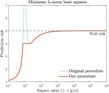
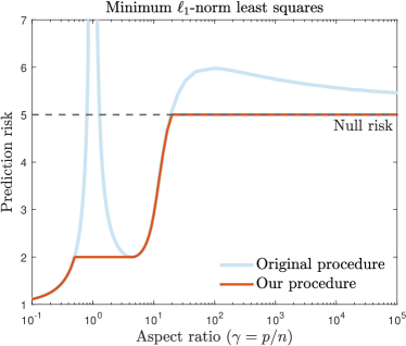
Figure 1: Monotonized asymptotic conditional prediction risk of the zero-step procedure (described in Algorithm 2) for the minimum $\ell_{2}$-norm and $\ell_{1}$-norm least squares procedures. The figure in the left panel follows the setup of Figure 2 of Hastie et al., (2019), and the figure in the right panel follows the setup of Figure 3 of Li and Wei, (2021) (at sparsity level = 0.01). Both settings assume isotropic features and a linear model with noise variance $\sigma^{2}=1$ and linear coefficients of squared Euclidean norm $\rho^{2}=4$. Note that the risk is lower bounded by $\sigma^{2}=1$ and the risk of the null predictor (null risk) is $\rho^{2}+\sigma^{2}=5$.

Figure 1 illustrates the above result for the minimum $\ell_{2}$-norm least squares estimator (Hastie et al.,, 2019) and the minimum $\ell_{1}$-norm least squares estimator (Li and Wei,, 2021). The light-blue lines show the asymptotic risk profiles of the two procedures, which are non-monotonic as they diverge to infinity around the interpolation threshold of $1$, at which the sample size and the number of features are equal. The red lines depict the risk profiles of the zero-step procedure ${\widehat{f}}^{\mathrm{zs}}$, which corresponds to the map

$$\gamma\in(0,\infty)~{}\mapsto~{}\min_{\zeta\geq\gamma}R^{\mathrm{det}}(\zeta;{\widehat{f}}).$$ (1)

The function (1) is a monotonically non-decreasing function of $\gamma$, regardless of whether $\gamma\mapsto R^{\mathrm{det}}(\gamma;{\widehat{f}})$ is non-monotonic. Furthermore, since

$$\smash{\min_{\zeta\geq\gamma}R^{\mathrm{det}}(\zeta;{\widehat{f}})\leq R^{\mathrm{det}}(\gamma;{\widehat{f}})},\mbox{ for all }\gamma>0,$$

the asymptotic risk of ${\widehat{f}}^{\mathrm{zs}}$ is no worse than that of ${\widehat{f}}$. We refer to the function described in (1) as the monotonized risk of the base procedure ${\widehat{f}}$.

The assumptions required in Theorem 1.1 are very mild, and apply to a broad range of procedures and settings. Indeed, as remarked above, the risk profile $R^{\mathrm{det}}(\cdot;{\widehat{f}})$ of several estimators have been recently identified under proportional asymptotics regime; see Remark 3.16. The requirements on the loss functions are also mild and can be verified for common loss functions. In fact, our results do not require proportional asymptotics and hold more generally.

We also develop a more sophisticated methodology whose asymptotic risk profile is not only monotonic in the aspect ratio but can be strictly smaller than the monotonized risk profile (1), a fact that we again verify for the minimum $\ell_{2}$, $\ell_{1}$-norm least squares procedures. See Section 4.

Core idea: the zero-step procedure.

Our methodology is conceptually straightforward, as it relies on a combination of sample splitting, sub-sampling, and cross-validation. The core principle is as follows. Starting off with an aspect ratio of $p/n$, if the risk were to be lower at, say, twice this aspect ratio $2p/n$, then we could just use half the data to evaluate the predictor, enjoying a smaller risk than the one obtained when training with the entire data. To decide whether the out-of-sample error is lower at any larger aspect ratio, we use cross-validation to “glean at” the values of the risk function at all aspect ratios larger than the one for the full data. To elaborate, we next give an informal description of one of our main methods, the zero-step procedure that we study in Section 3.

We initially split the data into a training and a validation set in such a way that the size of the validation set is a vanishing proportion of that of the training set. In the first step, we compute a collection of predictors, each resulting from applying the same base prediction procedure on a sub-sample of size $k_{n}$ varying over a grid of values in $\mathcal{K}_{n}$. Depending on the size of the sub-sample, we are able to mimic the behavior of the risk at larger aspect ratios ($p/k_{n}$, $k_{n}\in\mathcal{K}_{n}$). In the second step, we estimate the out-of-sample risk of each of these predictors using the validation set. With $\{p/k_{n}:k_{n}\in\mathcal{K}_{n}\}$ approximating the set $[p/n,\infty]$, these estimated out-of-sample risks act as proxies for the true generalization error at larger aspect ratios. In the final step, we perform model selection by minimizing the estimated test error across the candidate aspect ratios. In order to make full use of the data, one can use more than one sub-sample for each $k_{n}\in\mathcal{K}_{n}$, a practice that closely resembles bagging. To prove the “correctness” of the split-sample cross-validation, we develop novel oracle inequalities in additive and multiplicative forms that are of independent interest.

Because the core components of our approach are sub-sampling and cross-validation, our methodology is applicable to virtually any algorithm – even the black-box type – and its validity holds under minimal assumptions on the data generating distribution.

1.1 Summary of results

Below we summarize the main contributions of this paper.

• Novel guarantees for split-sample cross-validation. At its core, our methodology performs model selection of arbitrary learning procedures built over sub-samples of different sizes, with the size of the sub-samples treated as a tuning parameter to optimize. Towards that goal, we rely on split-sample cross-validation, which we analyze in Section 2. In Proposition 2.1, we provide deterministic inequalities for the risk of split cross-validated predictors in both additive and multiplicative form. We remark that multiplicative oracle inequalities allow for the possibility of unbounded oracle risk values, and are therefore well suited to incorporate prediction procedures exhibiting the double descent phenomena around the interpolating threshold. Leveraging concentration inequalities for both the mean estimator of the prediction risk and the median-of-means estimator, in Section 2.3, we show how these bounds imply finite-sample oracle inequalities for split-sample cross-validation that are applicable to a broad range of loss functions and under minimal assumptions on the learning procedure. In particular, our results do not require well-specified (parametric) models. We exemplify our bounds on various loss functions for both regression and classification, and in Theorem 2.22, we give a general multiplicative oracle inequality for arbitrary linear predictors under mild distributional assumptions.

• Zero-step procedure. Using oracle inequalities for split-sample cross-validation, we put forth a general methodology that takes as input an arbitrary prediction procedure and minimizes the prediction risk of its bagged version over a grid of sub-sample sizes. We call this the “zero-step” prediction procedure. We analyze the asymptotic risk behavior of the zero-step procedure under proportional asymptotics, in which the number of features grows proportionally with the number of observations. In Theorem 3.11, we prove that the risk of predictor returned by the zero-step procedure is upper bounded by the monotonized risk given in (1). Unlike most contributions in the literature on over-parameterized learning, our results do not depend on well-specified (parametric) models and only require the existence of a sufficiently well-behaved asymptotic risk profile.

• One-step procedure. In Section 4, we further generalize the zero-step procedure by considering an adjustment of the original predictor that is inspired by the one-step estimation method used in parametric statistics to improve efficiency (Van der Vaart,, 2000, Section 5.7). This modification, which can be thought of as a single-iterate boosting of the baseline procedure, is shown, both in theory and in simulations, to produce an asymptotic monotonized risk that is smaller than the monotonized risk of the zero-step procedure; see Theorem 4.4. We derive explicit expressions of the asymptotic risk profile of the one-step procedure for the minimum $\ell_{2}$, $\ell_{1}$-norm least squares prediction procedures. The main insight we draw from the minimum $\ell_{2}$-norm least squares example is that the one-step procedure in addition to changing the aspect ratio of the predictor also reduces the signal energy leading to a smaller asymptotic risk; see Remark 4.12.

• Risk profiles. In our study of the performance of the zero-step and one-step procedures, we derive several auxiliary results that might of independent interest. Specifically, we provide a systematic way to certify the continuity or lower semicontinuity of the asymptotic risk profile of any prediction procedure, assuming only point-wise convergence of the conditional prediction risk under proportional asymptotics; see Proposition 3.10. This is often hard to prove directly from the asymptotic risk profiles as they are usually defined implicitly via one or more fixed-point equations. Also of independent interest is a representation that we prove, for the conditional prediction risk of an arbitrary linear predictor with a one-iterate boosting with minimum $\ell_{2}$-norm least squares, using the recent tools from random matrix theory. This, in particular, involves deriving deterministic equivalents for the generalized bias and variance of the ridgeless predictor which may be of independent interest; see Lemmas S.5.3 and 4.8.

We corroborate our theoretical results with several illustrative simulations. An intriguing finding emerging from our numerical studies is the fact that bagging, i.e., aggregation over sub-sample, appears to have a significant positive impact on the asymptotic risk profile of both the zero- and one-step procedure: averaging over an increasing number of sub-samples results in a downward shift of the risk asymptotic profile, especially around the interpolation threshold: see, e.g., Figures 4 and 3. Though we do not provide a theoretical justification for this interesting phenomenon, we offer some conjectures in the discussion section; see Section 5.

1.2 Other related work

In this section, we review some related work on risk non-monotonicity, cross-validation, as well as exact asymptotic risk characterization. Explicit references to these works, when appropriate, are also made in the main sections of the paper.

Non-monotonicity of generalization performance.

The study of non-monotone risk behavior is largely motivated by empirical evidence in standard statistical learning tasks such as classification and prediction, where instances of non-monotonic risk profiles were originally discovered and reported. See Trunk, (1979); Duin, (1995); Opper and Kinzel, (1996) and Loog et al., (2020) for some earlier findings on the double descent risk behavior. Recently, it has garnered growing interest due to the remarkable successes of neural networks where similar non-monotonic behavior has also been observed; see LeCun et al., (1990); Geiger et al., (2019); Zhang et al., (2017, 2021) and references therein. The non-monotonic behavior of the test error as a function of the model size in general context was brought up by Belkin et al., 2019a and has since been theoretically established for many other classical estimators such as linear/kernel regression, ridge regression, logistic regression, and under stylized models such as linear model or random features model. Besides the work discussed in our main sections, see also Kini and Thrampoulidis, (2020); Mei and Montanari, (2019); Mitra, (2019); Derezinski et al., (2020); Frei et al., (2022) and the survey paper Bartlett et al., (2021). When it comes to the sample-wise non-monotonic performances, a recent line of work asks and provides partial answers to the question: given additional observation points, when and to what extend will the generalization performance improve (Viering et al.,, 2019; Nakkiran,, 2019; Nakkiran et al.,, 2020; Mhammedi,, 2021). In particular, Nakkiran et al., (2020) investigates the role of optimal tuning in the context of ridge regression, and for a class of linear models, demonstrated that the optimally-tuned $\ell_{2}$ regularization achieves monotonic generalization performance.

Data-splitting and cross-validation.

The framework developed in the current paper crucially depends on split-sample cross-validation, which compares different predictors trained on one part of the sample using out-of-sample risk estimates from the remaining part. The split-sample cross-validation is a well-known methodology studied in several works (e.g., Stone, (1974); Györfi et al., (2002); Yang, (2007); Arlot and Celisse, (2010)). Split-sample cross-validation is theoretically easier to analyze compared to the $k$-fold cross-validation and is shown to yield optimal rates in the context of non-parametric regression (Yang,, 2007; Van der Laan et al.,, 2007; Van der Vaart et al.,, 2006). These works have derived oracle inequalities that show that split-sample cross-validation based predictor has asymptotically the smallest risk among the collection of predictors up to an additive error (that converges to zero). The oracle inequalities are either called exact or inexact depending on whether the constant multiplying the smallest risk is 1 or $1+\delta$ (for an arbitrarily $\delta$); see, e.g., Lecué and Mendelson, (2012). All these works have used split-sample cross-validation for the purpose of choosing predictors with good prediction risk, and the existing oracle inequalities are all additive in nature.

Application of cross-validation for over-parameterized learning is more recent and here special care is required in choosing the split sizes because splitting in half would change the aspect ratios in the proportional asymptotics regime. In contrast to the low dimensional or non-parametric setting, it is well-known that the classical $k$-fold cross-validation framework suffers from severe bias and thus requires careful modification or a diverging choice of $k$ (see, e.g., Mücke et al., (2021); Rad and Maleki, (2020)). In particular, when $k$ is taken to be $n$, the resulting procedure is also known as leave-one-out cross-validation (LOOCV), which mitigates these bias issue and has proven to be effective in a variety of settings; see  Beirami et al., (2017); Wang et al., (2018); Giordano et al., (2019); Stephenson and Broderick, (2020); Wilson et al., (2020); Austern and Zhou, (2020); Xu et al., (2021); Patil et al., (2021, 2022) and references therein.

Our use of cross-validation is slightly different: the goal is to choose the “optimal” sub-sample size for a single prediction procedure. Furthermore, supplementing the existing oracle inequalities for cross-validation, we also provide a multiplicative oracle inequality which shows that the split-sample cross-validated predictor attains the smallest risk in the collection up to a factor converging to $1$ with the sample size. This multiplicative version is crucial for our study, allowing us to consider ingredient predictors whose risk might diverge with sample size.

Risk characterization.

In developing our zero-step and one-step procedures, we assume existence of a deterministic risk profile function for every aspect ratio. As discussed, the exact formulas for the risk profile functions have been obtained for various estimators in both classification and regression settings. In the past decade, several distinct techniques and tools have been developed to explicitly describe and analyze these risk functions. Prominent examples include the leave-one-out type perturbation analysis (e.g., Karoui, (2013, 2018)), the approximate message passing machinery (e.g., Donoho et al., (2009); Donoho and Montanari, (2016); Bayati and Montanari, (2011)), and the convex Gaussian min-max theorem (e.g., Stojnic, (2013); Thrampoulidis et al., (2015, 2018)). These techniques rely critically upon a well-specified model, as well as the assumption that the entries of the design matrix are drawn i.i.d. from standard normal distribution, while some restricted universality results are developed in Bayati et al., (2015); Montanari and Nguyen, (2017); Chen and Lam, (2021); Hu and Lu, (2020). In this work, however, we take a more direct approach and develop some non-asymptotic oracle risk inequalities. Leveraging upon these oracle inequalities, our results do not require well-specified models, and only assume the existence of a relatively well-behaved risk profile, which presumably allows for weaker distributional assumptions.

1.3 Organization and notation

Organization.

The rest of the paper is organized as follows.

• In Section 2, we describe the general cross-validation and model selection algorithm, derive associated oracle risk inequalities, and provide probabilistic bounds on the error terms. We then obtain concrete results for a variety of classification and regression loss functions.

• In Section 3, we describe the zero-step prediction procedure, and provide its risk monotonization guarantee. We then explicitly verify the related assumptions for the ridgeless and lassoless prediction procedures, and show corresponding numerical illustrations.

• In Section 4, we describe the one-step prediction procedure, and provide its risk monotonization guarantee. We then explicitly verify assumptions for arbitrary linear predictors, the special cases of ridgeless and lassoless prediction procedures, and show corresponding numerical illustrations.

• In Section 5, we conclude the paper and provide three concrete directions for future work.

Nearly all the proofs in the paper are deferred to the Supplementary Material. The sections and the equation numbers in the Supplementary Material are prefixed with the letters “S” and “E”, respectively.

Notation.

We use $\mathbb{N}$ to denote the set of natural numbers, $\mathbb{R}$ to denote the set of real numbers, $\mathbb{R}_{\geq 0}$ to denote the set of non-negative real numbers, $\mathbb{R}_{>0}$ to denote the set of positive real numbers, and $\overline{\mathbb{R}}$ to denote the extended real number system, i.e., $\overline{\mathbb{R}}=\mathbb{R}\cup\{-\infty,+\infty\}$. For a real number $a$, $(a)_{+}$ denotes its positive part, $\lfloor a\rfloor$ denotes its floor, $\lceil a\rceil$ denotes its ceiling. For a set $\mathcal{A}$, we use $\smash{\mathbbm{1}_{\mathcal{A}}}$ to denote its indicator function. We denote convergence in probability by $\smash{\xrightarrow{\text{p}}}$, almost sure convergence by $\smash{\xrightarrow{\text{a.s.}}}$, and weak convergence by $\smash{\xrightarrow{\text{d}}}$. We use generic letters $C,C_{1},C_{2},\dots$ to denote constants whose values may change from line to line.

For a comprehensive list of notation used in the paper, see Section S.9.

2 General cross-validation and model selection

The primary focus of this paper is to develop a framework to improve upon prediction procedures in the overparameterized regime in which the number of features $p$ is comparable to and often exceeds the number of observations $n$, and where the predictive risk may be non-monotonic in the aspect ratio $p/n$. As discussed in Section 1, a fundamental component of our methodology is the selection of an optimal size of the sub-samples through cross-validation. To that effect, we begin by deriving some general, non-asymptotic oracle risk inequalities for split-sample cross-validation, as described in Algorithm 1, that hold under minimal assumptions. While our bounds apply to a wide range of learning problems and may be of independent interest, they are crucial in demonstrating the risk monotonization properties of the procedures presented in Sections 3 and 4.

Though cross-validation is a well-known and well-studied procedure  (see, e.g., Van der Laan et al.,, 2007; Györfi et al.,, 2002; Yang,, 2007), our work extends the previous results on cross-validation in a couple of ways: (1) We derive two forms of oracle risk inequalities: the additive form that is better suited for bounded loss functions (especially classification losses), and the multiplicative form that is better suited unbounded loss functions (especially regression losses); (2) In addition to common sample mean based estimation of the prediction risk, we also analyze the median-of-means based estimation of the prediction risk that proves to be useful in relaxing strong moment assumption on the predictors.

Inputs:

• a dataset $\mathcal{D}_{n}=\{(X_{i},Y_{i})\in\mathbb{R}^{p}\times\mathbb{R}:1\leq i\leq n\}$;

• a positive integer $n_{\mathrm{te}}<n$;

• an index set $\Xi$;

• a set of prediction procedures $\{{\widehat{f}}^{\xi}$: $\xi\in\Xi\}$;

• a loss function $\ell:\mathbb{R}\times\mathbb{R}\to\mathbb{R}_{\geq 0}$;

• a centering procedure $\texttt{CEN}\in\{\texttt{AVG},\texttt{MOM}\}$;

• a real number $\eta>0$ if CEN is MOM.

Output:

• a predictor ${\widehat{f}}^{\mathrm{cv}}(\cdot;\mathcal{D}_{n}):\mathbb{R}^{p}\to\mathbb{R}$.

Procedure:

1. Randomly split the index set $\mathcal{I}_{n}=\{1,\dots,n\}$ into two disjoint sets $\mathcal{I}_{\mathrm{tr}}$ and $\mathcal{I}_{\mathrm{te}}$ such that $|\mathcal{I}_{\mathrm{tr}}|=n-n_{\mathrm{te}}$ (which we denote by $n_{\mathrm{tr}}$), $|\mathcal{I}_{\mathrm{te}}|=n_{\mathrm{te}}$. Denote the corresponding splitting of the dataset $\mathcal{D}_{n}$ by $\mathcal{D}_{\mathrm{tr}}=\{(X_{i},Y_{i}):i\in\mathcal{I}_{\mathrm{tr}}\}$ (for training) and $\mathcal{D}_{\mathrm{te}}=\{(X_{j},Y_{j}):j\in\mathcal{I}_{\mathrm{te}}\}$ (for testing).

2. For each $\xi\in\Xi$, fit the prediction procedure ${\widehat{f}}^{\xi}$ on $\mathcal{D}_{\mathrm{tr}}$ to obtain the predictor ${\widehat{f}}^{\xi}(\cdot;\mathcal{D}_{\mathrm{tr}}):\mathbb{R}^{p}\to\mathbb{R}$.

3. For each $\xi\in\Xi$,

• if $\texttt{CEN}~{}=~{}\texttt{AVG}$, estimate the conditional prediction risk of ${\widehat{f}}^{\xi}$ using

  $${\widehat{R}}({\widehat{f}}^{\xi}(\cdot;\mathcal{D}_{\mathrm{tr}}))=\frac{1}{|\mathcal{D}_{\mathrm{te}}|}\sum_{j\in\mathcal{I}_{\mathrm{te}}}\ell(Y_{j},{\widehat{f}}^{\xi}(X_{j};\mathcal{D}_{\mathrm{tr}})).$$ (2)

• if $\texttt{CEN}~{}=~{}\texttt{MOM}$, estimate the conditional prediction risk of ${\widehat{f}}^{\xi}$ using

  $${\widehat{R}}({\widehat{f}}^{\xi}(\cdot;\mathcal{D}_{\mathrm{tr}}))=\texttt{MOM}\big{(}\big{\{}\ell(Y_{j},{\widehat{f}}^{\xi}(X_{j};\mathcal{D}_{\mathrm{tr}})),\,j\in\mathcal{I}_{\mathrm{te}}\big{\}},\,\eta\big{)}.$$ (3)

  See discussion after Lemma S.8.2 for the definition of $\texttt{MOM}(\cdot,\cdot)$.

Set $\widehat{\xi}\in\Xi$ to be the index that minimizes the estimated prediction risk using

$$\widehat{\xi}\in\mathop{\mathrm{arg\,min}}_{\xi\in\Xi}{\widehat{R}}({\widehat{f}}^{\xi}(\cdot;\mathcal{D}_{\mathrm{tr}})).$$ (4)

Note that $\widehat{\xi}$ need not be unique (hence the set notation) and any choice that leads to the minimum estimated risk enjoys the subsequent theoretical guarantees in the paper.

Return the predictor ${\widehat{f}}^{\mathrm{cv}}(\cdot;\mathcal{D}_{n})={\widehat{f}}^{\widehat{\xi}}(\cdot;\mathcal{D}_{\mathrm{tr}})$.

Algorithm 1 General cross-validation and model selection procedure

2.1 Oracle risk inequalities

Setting the stage, suppose we are given $n$ samples of labeled data $\mathcal{D}_{n}=\{(X_{1},Y_{1}),(X_{2},Y_{2}),\dots,(X_{n},Y_{n})\}$, where $X_{i}\in\mathbb{R}^{p}$ is a $p$-dimensional feature vector and $Y_{i}\in\mathbb{R}$ is a scalar response variable for $i=1,\dots,n$. Let ${\widehat{f}}$ be a prediction procedure that maps $\mathcal{D}_{n}$ to a predictor ${\widehat{f}}(\cdot;\mathcal{D}_{n}):\mathbb{R}^{p}\to\mathbb{R}$ (a measurable function of the data $\mathcal{D}_{n}$). For any predictor ${\widehat{f}}(\cdot;\mathcal{D}_{n})$, trained on the data set $\mathcal{D}_{n}$, that takes in a feature vector $x\in\mathbb{R}^{p}$ and outputs a real-valued prediction ${\widehat{f}}(x;\mathcal{D}_{n})$, we measure its predictive accuracy via a non-negative loss function $\ell:\mathbb{R}\times\mathbb{R}\to\mathbb{R}_{\geq 0}$. Given a new feature vector $X_{0}\in\mathbb{R}^{p}$ with associated response variable $Y_{0}\in\mathbb{R}$ so that $(X_{0},Y_{0})$ is independent of $\mathcal{D}_{n}$, the prediction error or out-of-sample error incurred by ${\widehat{f}}(\cdot;\mathcal{D}_{n})$ is $\ell(Y_{0},{\widehat{f}}(X_{0};\mathcal{D}_{n}))$. Note that the prediction error $\ell(Y_{0},{\widehat{f}}(X_{0};\mathcal{D}_{n}))$ is a random variable that is a function of both $\mathcal{D}_{n}$ and $(X_{0},Y_{0})$.

We will quantify the performance of ${\widehat{f}}(\cdot;\mathcal{D}_{n})$ using the conditional expected prediction loss. The conditional expected prediction loss given the data $\mathcal{D}_{n}$, or the conditional prediction risk for short, of ${\widehat{f}}(\cdot;\mathcal{D}_{n})$ is defined as

$$R({\widehat{f}}(\cdot;\mathcal{D}_{n}))~{}:=~{}\mathbb{E}_{X_{0},Y_{0}}[\ell(Y_{0},{\widehat{f}}(X_{0};\mathcal{D}_{n}))\mid\mathcal{D}_{n}]~{}=~{}\int\ell(y,{\widehat{f}}(x;\mathcal{D}_{n}))\;\mathrm{d}P(x,y),$$ (5)

where $P$ denotes the joint probability distribution of $(X_{0},Y_{0})$. Note that $R({\widehat{f}}(\cdot;\mathcal{D}_{n}))$ is a random variable that depends on $\mathcal{D}_{n}$. An empirical estimator of $R({\widehat{f}}(\cdot;\mathcal{D}_{n}))$ is denoted by ${\widehat{R}}({\widehat{f}}(\cdot;\mathcal{D}_{n}))$. In this paper, we mainly consider two such estimators: the average estimator and the median-of-means estimator as defined in (2) and (3), respectively.

Consider any prescribed index set $\Xi$, where each $\xi\in\Xi$ corresponds to a specific model that will be clear from the context. Based on the training data, a predictor ${\widehat{f}}^{\xi}(\cdot;\mathcal{D}_{\mathrm{tr}})$ is fitted for each model $\xi$ and estimated risks of ${\widehat{f}}^{\xi}$, $\xi\in\Xi$ are compared on a validation data set as described in Algorithm 1. Let ${\widehat{f}}^{\mathrm{cv}}(\cdot;\mathcal{D}_{n})$ be the final predictor returned by Algorithm 1. We shall consider two types of oracle inequalities: one in an additive form and the other in a multiplicative form. More specifically, for any prescribed model set $\Xi$, define the additive error term and multiplicative error term respectively as follows:

$$\Delta_{n}^{\mathrm{add}} :=\max_{\xi\in\Xi}\Big{|}{\widehat{R}}({\widehat{f}}^{\xi}(\cdot;\mathcal{D}_{\mathrm{tr}}))-R({\widehat{f}}^{\xi}(\cdot;\mathcal{D}_{\mathrm{tr}}))\Big{|},$$ (6a)

$$\Delta_{n}^{\mathrm{mul}} :=\max_{\xi\in\Xi}\Big{|}\frac{{\widehat{R}}({\widehat{f}}^{\xi}(\cdot;\mathcal{D}_{\mathrm{tr}}))}{R({\widehat{f}}^{\xi}(\cdot;\mathcal{D}_{\mathrm{tr}}))}-1\Big{|}.$$ (6b)

The following proposition relates the performance of ${\widehat{f}}^{\mathrm{cv}}(\cdot;\mathcal{D}_{n})$ to the “oracle” prediction risk in terms of these errors terms.

Proposition 2.1 (Deterministic oracle risk inequalities).

The prediction risk of ${\widehat{f}}^{\mathrm{cv}}(\cdot;\mathcal{D}_{n})$ satisfies the following deterministic oracle inequalities:

1. additive form:

   $$\begin{split}R({\widehat{f}}^{\mathrm{cv}}(\cdot;\mathcal{D}_{n}))~{}&\leq~{}\min_{\xi\in\Xi}R({\widehat{f}}^{\xi}(\cdot;\mathcal{D}_{\mathrm{tr}})+2\Delta_{n}^{\mathrm{add}},\\ \mathbb{E}[R({\widehat{f}}^{\mathrm{cv}}(\cdot;\mathcal{D}_{n}))]~{}&\leq~{}\min_{\xi\in\Xi}\mathbb{E}[R({\widehat{f}}^{\xi}(\cdot;\mathcal{D}_{\mathrm{tr}})]+2\mathbb{E}[\Delta_{n}^{\mathrm{add}}].\end{split}$$ (7)

2. multiplicative form:

   $$R({\widehat{f}}^{\mathrm{cv}}(\cdot;\mathcal{D}_{n}))~{}\leq~{}\frac{1+\Delta_{n}^{\mathrm{mul}}}{(1-\Delta_{n}^{\mathrm{mul}})_{+}}\cdot\min_{\xi\in\Xi}R({\widehat{f}}^{\xi}(\cdot;\mathcal{D}_{\mathrm{tr}}).$$ (8)

Proposition 2.1 provides oracle bounds on the prediction risk of ${\widehat{f}}^{\mathrm{cv}}(\cdot;\mathcal{D}_{n})$ in terms of the error terms $\Delta_{n}^{\mathrm{add}}$ and $\Delta_{n}^{\mathrm{mul}}$. Note that Proposition 2.1 does not make any assumptions about the underlying model of the data or the dependence structure between the observations. Under some general conditions on the data, one can show that $\Delta_{n}^{\mathrm{add}}$ and/or $\Delta_{n}^{\mathrm{mul}}$ converge to zero in probability as $n\to\infty$. The exact rate of convergence depends on the number of observations $n_{\mathrm{te}}$ in the test data and also on the tail behavior of $\ell(Y_{0},\widehat{f}^{\xi}(X_{0};\mathcal{D}_{\mathrm{tr}}))$ conditional on $\widehat{f}^{\xi}(\cdot;\mathcal{D}_{\mathrm{tr}})$. For notational convenience, from now, we will write ${\widehat{f}}^{\mathrm{cv}}$ and ${\widehat{f}}^{\xi}$ to denote ${\widehat{f}}^{\mathrm{cv}}(\cdot;\mathcal{D}_{n})$ and ${\widehat{f}}^{\xi}(\cdot;\mathcal{D}_{\mathrm{tr}})$, respectively.

Remark 2.2 (Lower bound on $R({\widehat{f}}^{\mathrm{cv}})$).

Proposition 2.1 provides upper bounds on the (conditional) prediction risk of ${\widehat{f}}^{\mathrm{cv}}$ in terms of the minimum risk of ${\widehat{f}}^{\xi}$. It can be readily seen that the risk of ${\widehat{f}}^{\mathrm{cv}}$ is always lower bounded by the minimum risk. More formally, note that ${\widehat{f}}^{\mathrm{cv}}=\sum_{\xi\in\Xi}{\widehat{f}}^{\xi}\mathbbm{1}_{{\widehat{\xi}}=\xi}$, and, therefore,

$$R({\widehat{f}}^{\mathrm{cv}})~{}=~{}\sum_{\xi\in\Xi}R({\widehat{f}}^{\xi})\mathbbm{1}_{{\widehat{\xi}}=\xi}~{}\geq~{}\min_{\xi\in\Xi}R({\widehat{f}}^{\xi})\sum_{\xi\in\Xi}\mathbbm{1}_{{\widehat{\xi}}=\xi}~{}=~{}\min_{\xi\in\Xi}R({\widehat{f}}^{\xi}).$$

Combined with Proposition 2.1, we conclude that

$$\min_{\xi\in\Xi}R({\widehat{f}}^{\xi})~{}\leq~{}R({\widehat{f}}^{\mathrm{cv}})~{}\leq~{}\begin{cases}\min_{\xi\in\Xi}R({\widehat{f}}^{\xi})+\Delta_{n}^{\mathrm{add}}\\ \min_{\xi\in\Xi}R({\widehat{f}}^{\xi})\cdot(1+\Delta_{n}^{\mathrm{mul}})/(1-\Delta_{n}^{\mathrm{mul}})_{+}.\end{cases}$$

Thus, convergence (in probability) of either $\Delta_{n}^{\mathrm{add}}$ or $\Delta_{n}^{\mathrm{mul}}$ to $0$ implies that the risk of ${\widehat{f}}^{\mathrm{cv}}$ is asymptotically the same as the minimum risk of ${\widehat{f}}^{\xi}$, $\xi\in\Xi$ in either additive or multiplicative sense, respectively.

The additive and multiplicative form of oracle inequalities have their own advantages. Traditionally, the additive form is more common. The additive oracle inequality for the prediction risk readily implies the additive oracle inequality on the excess risk. In other words,

$$R({\widehat{f}}^{\mathrm{cv}})-R(f^{\star})\leq\min_{\xi\in\Xi}R({\widehat{f}}^{\xi})-R(f^{\star})+\Delta_{n}^{\mathrm{add}},$$

for any predictor $f^{\star}$. In particular, this will hold for the best (oracle) predictor for the prediction risk. This is not true of the multiplicative oracle inequality, which instead only implies the bound

$$R({\widehat{f}}^{\mathrm{cv}})-R(f^{\star})\leq c_{n}\big{\{}\min_{\xi\in\Xi}R({\widehat{f}}^{\xi})-R(f^{\star})\big{\}}+(c_{n}-1)R(f^{\star}),$$

where $f^{\star}$ is any predictor (in particular, the one with the best prediction risk) and

$$c_{n}=\frac{1+\Delta_{n}^{\mathrm{mul}}}{(1-\Delta_{n}^{\mathrm{mul}})_{+}},\quad c_{n}-1=\frac{2\Delta_{n}^{\mathrm{mul}}}{(1-\Delta_{n}^{\mathrm{mul}})_{+}}.$$

In terms of claiming that ${\widehat{f}}^{\mathrm{cv}}$ has prediction risk close to the best in the collection of predictors $\{{\widehat{f}}^{\xi},\xi\in\Xi\}$, the multiplicative form has certain advantages compared to the additive form. In the case that $\min_{\xi\in\Xi}R({\widehat{f}}^{\xi})$ converges to $0$, the additive oracle inequality (7) implies that the risk of the selected predictor $\widehat{f}^{\mathrm{cv}}$ asymptotically matches the risk of the best predictor among the collection $\{\widehat{f}^{\xi},\xi\in\Xi\}$ only if $\Delta_{n}^{\mathrm{add}}$ converges to zero faster than $\min_{\xi\in\Xi}R(\widehat{f}^{\xi})$. If, however, $\Delta_{n}^{\mathrm{add}}$ converges to zero slower than the minimum risk in the collection, then the additive oracle inequality does not imply a favorable result. In this case, a multiplicative oracle inequality helps. As long as $\Delta_{n}^{\mathrm{mul}}$ converges to 0, the multiplicative oracle inequality implies that ${\widehat{f}}^{\mathrm{cv}}$ matches in risk with the best predictor in the collection, irrespective of whether the minimum risk converges to zero or not. Note that $\Delta_{n}^{\mathrm{add}}$ only controls the additive error of the risk estimator $\widehat{R}(\widehat{f}^{\xi})$, which is easier to control than the multiplicative error; think of controlling the error of sample mean of $\mbox{Bernoulli}(p)$ random variables with $p=p_{n}\to 0$; See Remark 2.12 for a more mathematical discussion. Even when $\min_{\xi\in\Xi}R({\widehat{f}}^{\xi})$ does not converge to zero, the multiplicative form might be advantageous compared to the additive form. Indeed, suppose that ${\widehat{f}}^{\xi_{0}}$ is in the collection and its risk diverges as $n\to\infty$. Then, it may not be true that

$$\big{|}{\widehat{R}}({\widehat{f}}^{\xi_{0}})-R({\widehat{f}}^{\xi_{0}})\big{|}\overset{p}{\to}0,$$

because both ${\widehat{R}}({\widehat{f}}^{\xi_{0}})$ and $R({\widehat{f}}^{\xi_{0}})$ are diverging. This implies that $\Delta_{n}^{\mathrm{add}}$ does not converge to $0$ and in fact, might diverge. However, the minimum risk in the collection could still be finite, and the additive oracle inequality fails to capture this. On the other hand, ${\widehat{R}}({\widehat{f}}^{\xi_{0}})/R({\widehat{f}}^{\xi_{0}})$ can still converge to $1$ as $n\to\infty$ even if $R({\widehat{f}}^{\xi_{0}})$ diverges to $\infty$. In our applications in overparameterized learning, we will encounter this situation where the number of features ($p$) is close to the number of observations ($n$), i.e., $p/n\approx 1$. See Remark 2.23 for more details.

Remark 2.3 (From multiplicative to additive oracle inequality).

Note that if $\Delta_{n}^{\mathrm{mul}}=o_{p}(1)$, then $(1+\Delta_{n}^{\mathrm{mul}})/(1-\Delta_{n}^{\mathrm{mul}})_{+}=1+O_{p}(1)\Delta_{n}^{\mathrm{mul}}=1+o_{p}(1)$, then the multiplicative oracle inequality (8) yields

$$R(\widehat{f}^{\mathrm{cv}})~{}\leq~{}(1+O_{p}(1)\Delta_{n}^{\mathrm{mul}})\min_{\xi\in\Xi}R(\widehat{f}^{\xi})~{}=~{}(1+o_{p}(1))\min_{\xi\in\Xi}R(\widehat{f}^{\xi}).$$

Observe that this multiplicative form can be converted into an additive form as

$$R(\widehat{f}^{\mathrm{cv}})~{}\leq~{}\min_{\xi\in\Xi}R(\widehat{f}^{\xi})~{}+~{}O_{p}(1)\Delta_{n}^{\mathrm{mul}}\min_{\xi\in\Xi}R(\widehat{f}^{\xi}),$$

where the second term on the right hand side is always smaller order compared to the first term as long as $\Delta_{n}^{\mathrm{mul}}$ converges in probability to zero.

From this discussion, it follows that one can choose a predictor with the best prediction risk in a collection if either $\Delta_{n}^{\mathrm{add}}$ or $\Delta_{n}^{\mathrm{mul}}$ converges in probability to zero. The application of Algorithm 1 for risk monotonizing procedures will be discussed in the next three sections. In the next two subsections, we provide some general sufficient conditions to verify $\Delta_{n}^{\mathrm{add}}=o_{p}(1)$ and $\Delta_{n}^{\mathrm{mul}}=o_{p}(1)$ for independent data. We also provide examples of common loss functions and show that under some mild moment assumptions, they satisfy $\Delta_{n}^{\mathrm{add}}=o_{p}(1)$ and $\Delta_{n}^{\mathrm{mul}}=o_{p}(1)$.

2.2 Control of $\Delta_{n}^{\mathrm{add}}$ and $\Delta_{n}^{\mathrm{mul}}$

In order to characterize $R({\widehat{f}}^{\mathrm{cv}})$, by Proposition 2.1 it is sufficient to control $\Delta_{n}^{\mathrm{add}}$ and $\Delta_{n}^{\mathrm{mul}}$. In this section, we demonstrate that under certain assumptions on the loss function $\ell$, the error terms are small both in probability and in expectation, which in turn yields optimality of ${\widehat{f}}^{\mathrm{cv}}$ among the predictors in $\{\widehat{f}^{\xi},\xi\in\Xi\}$.

To facilitate our discussion, for each $\xi\in\Xi$, define the conditional $\psi_{1}$-Orlicz norm of $\ell(Y_{0},{\widehat{f}}^{\xi}(X_{0}))$ given $\mathcal{D}_{n}$ as

$$\|\ell(Y_{0},{\widehat{f}}^{\xi}(X_{0}))\|_{\psi_{1}\mid\mathcal{D}_{n}}:=\inf\big{\{}C>0:\,\mathbb{E}\big{[}\exp\big{(}|\ell(Y_{0},{\widehat{f}}^{\xi}(X_{0}))|/C\big{)}\mid\mathcal{D}_{n}\big{]}\leq 2\big{\}}.$$ (9)

Similarly, for $r\geq 1$, define the conditional $L_{r}$-norm as

$$\|\ell(Y_{0},{\widehat{f}}^{\xi}(X_{0}))\|_{L_{r}\mid\mathcal{D}_{n}}:=\big{(}\mathbb{E}\big{[}\big{|}\ell(Y_{0},{\widehat{f}}^{\xi}(X_{0}))\big{|}^{r}\mathrel{\big{|}}\mathcal{D}_{n}\big{]}\big{)}^{1/r}.$$ (10)

It is well-known (Vershynin,, 2018, Proposition 2.7.1) that

$$\|\ell(Y_{0},\widehat{f}^{\xi}(X_{0}))\|_{\psi_{1}|\mathcal{D}_{n}}~{}\asymp~{}\sup_{r\geq 1}r^{-1}\|\ell(Y_{0},\widehat{f}^{\xi}(X_{0}))\|_{L_{r}|\mathcal{D}_{n}},$$

i.e., there are absolute constants $C_{l}$ and $C_{u}$ such that

$$0<C_{l}\leq\frac{\|\ell(Y_{0},{\widehat{f}}^{\xi}(X_{0}))\|_{\psi_{1}\mid\mathcal{D}}}{\sup_{r\geq 1}r^{-1}\|\ell(Y_{0},{\widehat{f}}^{\xi}(X_{0}))\|_{L_{r}\mid\mathcal{D}_{n}}}\leq C_{u}<\infty.$$

2.2.1 Control of $\Delta_{n}^{\mathrm{add}}$

Let ${\widehat{f}}^{\xi}$, $n_{\mathrm{te}}$, and CEN be as defined in Algorithm 1, and $\Delta_{n}^{\mathrm{add}}$ be as defined in (6a).

Lemma 2.4 (Control of $\Delta_{n}^{\mathrm{add}}$ and its expectation for losses with bounded conditional $\psi_{1}$ norm).

Suppose $(X_{i},Y_{i}),i\in\mathcal{I}_{\mathrm{te}}$ are sampled i.i.d. from $P$. Suppose the loss function $\ell$ is such that

$$\|\ell(Y_{0},{\widehat{f}}^{\xi}(X_{0}))\|_{\psi_{1}\mid\mathcal{D}_{n}}\leq\widehat{\sigma}_{\xi}$$

for $(X_{0},Y_{0})\sim P$ and set $\widehat{\sigma}_{\Xi}:=\max_{\xi\in\Xi}\widehat{\sigma}_{\xi}$. Fix any $0<A<\infty$. Then, for $\texttt{CEN}=\texttt{AVG}$, or $\texttt{CEN}=\texttt{MOM}$ with $\eta=n^{-A}/|\Xi|$, there exists an absolute constant $C_{1}>0$ such that

$$\mathbb{P}\left(\Delta_{n}^{\mathrm{add}}\geq C_{1}\widehat{\sigma}_{\Xi}\max\left\{\sqrt{\frac{\log\left(|\Xi|n^{A}\right)}{n_{\mathrm{te}}}},\frac{\log\left(|\Xi|n^{A}\right)}{n_{\mathrm{te}}}\right\}\right)\leq n^{-A}.$$

Additionally, if for some $A>0$, there exists a $C_{2}>0$ such that $\mathbb{P}(\widehat{\sigma}_{\Xi}\geq C_{2})\leq n^{-A}$, then there exists an absolute constant $C_{3}>0$ such that

$$\begin{split}\mathbb{E}[\Delta_{n}^{\mathrm{add}}]&\leq C_{1}C_{2}\max\left\{\sqrt{\frac{\log\left(|\Xi|n^{A}\right)}{n_{\mathrm{te}}}},\frac{\log\left(|\Xi|n^{A}\right)}{n_{\mathrm{te}}}\right\}+C_{3}n^{-A/r}|\Xi|^{1/t}\max\left\{\sqrt{\frac{t}{n_{\mathrm{te}}}},\frac{t}{n_{\mathrm{te}}}\right\}\max_{\xi\in\Xi}\|\widehat{\sigma}_{\xi}\|_{L_{t}}\end{split}$$ (11)

for every $r,t\geq 2$ and $1/r+1/t=1$.

Lemma 2.5 (Control of $\Delta_{n}^{\mathrm{add}}$ and its expectation for losses with bounded conditional $L_{2}$ norm).

Suppose $(X_{i},Y_{i}),i\in\mathcal{I}_{\mathrm{te}}$ are sampled i.i.d. from $P$. Suppose the loss function $\ell$ is such that

$$\|\ell(Y_{0},{\widehat{f}}^{\xi}(X_{0}))\|_{L_{2}\mid\mathcal{D}_{n}}\leq\widehat{\sigma}_{\xi}$$

for $(X_{0},Y_{0})\sim P$ and set $\widehat{\sigma}_{\Xi}:=\max_{\xi\in\Xi}\widehat{\sigma}_{\xi}$. Fix any $0<A<\infty$. Then, for $\texttt{CEN}=\texttt{MOM}$ with $\eta=n^{-A}/|\Xi|$, there exists an absolute constant $C_{1}>0$ such that

$$\mathbb{P}\left(\Delta_{n}^{\mathrm{add}}\geq C_{1}\widehat{\sigma}_{\Xi}\sqrt{\frac{\log(|\Xi|n^{A})}{n_{\mathrm{te}}}}\right)\leq n^{-A}.$$ (12)

Additionally, if for some $A>0$ there exists a $C_{2}>0$ such that $\mathbb{P}(\widehat{\sigma}_{\Xi}\geq C_{2})\leq n^{-A}$, then for $\texttt{CEN}=\texttt{MOM}$,

$$\mathbb{E}\left[\Delta_{n}^{\mathrm{add}}\right]\leq C_{1}C_{2}\sqrt{\frac{\log(|\Xi|n^{A})}{n_{\mathrm{te}}}}+C_{3}n^{-A/2}|\Xi|^{1/2}\sqrt{\frac{\log^{2}(|\Xi|n^{A})}{n_{\mathrm{te}}}}\max_{\xi\in\Xi}\|\widehat{\sigma}_{\xi}\|_{L_{2}}$$ (13)

for some absolute constant $C_{3}>0$.

Remark 2.6 (Comparison of assumptions for $\texttt{CEN}=\texttt{AVG}$ and $\texttt{CEN}=\texttt{MOM}$.).

Comparing Lemmas 2.4 and 2.5, we note that the median-of-means method of risk estimation only requires control of the $L_{2}$ moments of the loss function compared to the $\psi_{1}$ (exponential) moments of the loss function. This is not surprising given that the median-of-means was developed as a sub-Gaussian estimator of the mean, only assuming finite variance (Lemma S.8.2). The $L_{2}$ moment assumption in Lemma 2.5 can be further relaxed to an $L_{1+\alpha}$ moment assumption for $\alpha\in(0,1]$ (Lugosi and Mendelson,, 2019, Theorem 3) at the cost of weaker rate of convergence of $\Delta_{n}^{\mathrm{add}}$. One can, of course, replace the median-of-means estimator with any other sub-Gaussian or sub-exponential mean estimator (Catoni,, 2012; Minsker,, 2015; Fan et al.,, 2017) and obtain a similar weakening of the moment assumptions. Same remark continues to hold for $\Delta_{n}^{\mathrm{mul}}$ discussed in Section 2.2.2.

Remark 2.7 (Restriction on $A$ for $\texttt{CEN}=\texttt{MOM}$).

In Lemmas 2.4 and 2.5, we allow for a free parameter $A$. However, in order for the choice of $\eta$ to be feasible in the MOM construction (see, e.g., Lemma S.8.2 in Section S.8), we need $B=\lceil 8\log(1/\eta)\rceil\leq n_{\mathrm{te}}$, which puts the following constraint on $A$:

$$8\log(n^{A}|\Xi|)\leq n_{\mathrm{te}}\quad\iff\quad A\log n\leq\frac{n_{\mathrm{te}}}{8}-\log(|\Xi|)\quad\iff\quad A\leq\frac{n_{\mathrm{te}}}{8\log n}-\frac{\log(|\Xi|)}{\log n}.$$

For a large enough $n$, this allows for a large range of $A$. In addition, the right hand side is large enough to imply exponentially small probability bound for the event that $\Delta_{n}^{\mathrm{add}}$ is large. The same remark holds for Lemmas 2.9 and 2.10 below.

The key quantities that drive the tail probability and expectation bound on $\Delta_{n}^{\mathrm{add}}$ in both Lemmas 2.4 and 2.5 are $\widehat{\sigma}_{\Xi}$ and $|\Xi|$. The following remark specifies the permissible growth rates on $\widehat{\sigma}_{\Xi}$ and $|\Xi|$ to ensure that $\Delta_{n}^{\mathrm{add}}$ is asymptotically small in probability.

Remark 2.8 (Tolerable growth rates on $\widehat{\sigma}_{\Xi}$ for $\Delta_{n}^{\mathrm{add}}=o_{p}(1)$).

Suppose $|\Xi|\leq n^{S}$ for some constant $S>0$ independent of $n,p$. If

$$\widehat{\sigma}_{\Xi}=o_{p}\left(\sqrt{\frac{n_{\mathrm{te}}}{\log n}}\right),$$

then under the setting of Lemmas 2.4 and 2.5, $\Delta_{n}^{\mathrm{add}}=o_{p}(1)$ as $n\to\infty$. The remark follows simply by noting that the dominating term in the probabilistic bound on $\Delta_{n}^{\mathrm{add}}$ in (12) is of order

$$\widehat{\sigma}_{\Xi}\sqrt{\frac{\log(|\Xi|n^{A})}{n_{\mathrm{te}}}}\leq\widehat{\sigma}_{\Xi}\sqrt{\frac{(S+A)\log n}{n_{\mathrm{te}}}}=O\left(\widehat{\sigma}_{\Xi}\sqrt{\frac{\log n}{n_{\mathrm{te}}}}\right).$$

See Section S.6.9 for feasible rates for $\widehat{\sigma}_{\Xi}$ to ensure that $\mathbb{E}[\Delta_{n}^{\mathrm{add}}]=o(1)$.

2.2.2 Control of $\Delta_{n}^{\mathrm{mul}}$

Moving on to $\Delta_{n}^{\mathrm{mul}}$, analogously to Lemmas 2.4 and 2.5, the following results provide high probability bounds on $\Delta_{n}^{\mathrm{mul}}$ in terms of a coefficient of variation parameter $\kappa$ which is the relative standard deviation of $\ell(Y_{0},\widehat{f}^{\xi}(X_{0}))$ conditional on $\mathcal{D}_{n}$. Let ${\widehat{f}}^{\xi}$, $n_{\mathrm{te}}$, CEN be as defined Algorithm 1, and $\Delta_{n}^{\mathrm{mul}}$ be as in (6b).

Lemma 2.9 (Control of $\Delta_{n}^{\mathrm{mul}}$ for losses with bounded conditional $\psi_{1}$ norm).

Suppose $(X_{j},Y_{j})$, $j\in\mathcal{I}_{\mathrm{te}}$ are sampled i.i.d. from $P$. Suppose the loss function $\ell$ is such that

$$\|\ell(Y_{0},{\widehat{f}}^{\xi}(X_{0}))\|_{\psi_{1}\mid\mathcal{D}_{n}}\leq\widehat{\sigma}_{\xi}~{}\text{ for }(X_{0},Y_{0})\sim P.$$

Define $\widehat{\kappa}_{\xi}=\widehat{\sigma}_{\xi}/R({\widehat{f}}^{\xi})$ and $\widehat{\kappa}_{\Xi}=\max_{\xi\in\Xi}\widehat{\kappa}_{\xi}$. Fix any $0<A<\infty$. Then, for $\texttt{CEN}=\texttt{AVG}$, or $\texttt{CEN}=\texttt{MOM}$ with $\eta=n^{-A}/|\Xi|$,

$$\mathbb{P}\left(\Delta_{n}^{\mathrm{mul}}\geq C\widehat{\kappa}_{\Xi}\max\left\{\sqrt{\frac{\log(|\Xi|n^{A})}{n_{\mathrm{te}}}},\frac{\log(|\Xi|n^{A})}{n_{\mathrm{te}}}\right\}\right)\leq n^{-A}$$

for a positive constant $C$.

Lemma 2.10 (Control of $\Delta_{n}^{\mathrm{mul}}$ for losses with bounded conditional $L_{2}$ norm).

Suppose $(X_{j},Y_{j})$, $j\in\mathcal{I}_{\mathrm{te}}$ are sampled i.i.d. from $P$. Suppose the loss function $\ell$ is such that

$$\|\ell(Y_{0},{\widehat{f}}^{\xi}(X_{0}))\|_{L_{2}\mid\mathcal{D}_{n}}\leq\widehat{\sigma}_{\xi}~{}\text{ for }(X_{0},Y_{0})\sim P.$$

Define $\widehat{\kappa}_{\xi}:=\widehat{\sigma}_{\xi}/R({\widehat{f}}^{\xi})$ and $\widehat{\kappa}_{\Xi}:=\max_{\xi\in\Xi}\widehat{\kappa}_{\xi}$. Fix any $0<A<\infty$. Then, for $\texttt{CEN}=\texttt{MOM}$ with $\eta=n^{-A}/|\Xi|$,

$$\mathbb{P}\left(\Delta_{n}^{\mathrm{mul}}\geq C\widehat{\kappa}_{\Xi}\sqrt{\frac{\log(|\Xi|n^{A})}{n_{\mathrm{te}}}}\right)\leq n^{-A}$$

for a positive constant $C$.

Remark 2.11 (Tolerable growth rate on $\widehat{\kappa}_{\Xi}$ for probabilistic bound).

Suppose $|\Xi|\leq n^{S}$ for some $S<\infty$. If

$$\widehat{\kappa}_{\Xi}=o_{p}\left(\sqrt{\frac{n_{\mathrm{te}}}{\log n}}\right),$$

then under the setting of Lemmas 2.9 and 2.10, $\Delta_{n}^{\mathrm{mul}}=o_{p}(1)$ as $n\to\infty$.

Remark 2.12 (Comparing the control of $\Delta_{n}^{\mathrm{add}}$ versus $\Delta_{n}^{\mathrm{mul}}$).

Note that from Lemmas 2.4 and 2.9, controlling $\Delta_{n}^{\mathrm{add}}$ requires controlling $\widehat{\sigma}_{\Xi}$, while controlling $\Delta_{n}^{\mathrm{mul}}$ requires controlling $\widehat{\kappa}_{\Xi}$. The former is on the scale of the standard deviation of the loss, while the latter is normalized standard deviation (where the normalization is with respect to the expectation of the loss). The advantage of the latter is that, even if the standard deviation diverges, the normalized standard deviation can be finite. This, in fact, happens for the case of minimum $\ell_{2}$-norm least squares predictor when $\gamma\approx 1$, in which case the control of $\Delta_{n}^{\mathrm{mul}}$ is feasible. See also the discussion in Remark 2.23.

Remark 2.13 (Choice of $n_{\mathrm{te}}$).

The above results hold true as long as $n_{\mathrm{te}}\to\infty$. Of course, the choice $n_{\mathrm{te}}$ restricts the allowable growth rate of $\widehat{\sigma}_{\Xi}$ and $\widehat{\kappa}_{\Xi}$ as discussed in Remarks 2.8 and 2.11. In our later applications in overparameterized learning, we adopt the proportional asymptotics framework in which the number of covariates to the number of observations converges to a non-zero constant. For this reason, we restrict ourselves to the choices of $n_{\mathrm{te}}$ such that $n_{\mathrm{te}}/n\to 0$ as $n\to\infty$; for example, one can take $n_{\mathrm{te}}=n^{\nu}$ for some $\nu<1$. This allows us to have training models with the same limiting aspect ratio (dimension/sample size) as that of the original data without splitting. However, the larger the $n_{\mathrm{te}}$, the more accurate our estimator of the prediction risk. For this reason, we suggest $n_{\mathrm{te}}=O(n/\log n)$ rather than $n_{\mathrm{te}}=n^{\nu}$.

2.3 Applications to loss functions

Below we consider several examples of common predictors and loss functions, and bound the corresponding conditional $\widehat{\sigma}$ parameters used in Lemmas 2.4 and 2.5, and conditional $\widehat{\kappa}$ parameters used in Lemmas 2.9 and 2.10. Recall the conditional $\psi_{1}$ and $L_{r}$ norms from (9) and (10), respectively. In addition, let $\psi_{2}$ denote the $\psi_{2}$-Orlicz norm.

Recall $\widehat{\sigma}_{\Xi}$ is the maximum of either $\|\ell(Y_{0},{\widehat{f}}^{\xi}(X_{0}))\|_{\psi_{1}\mid\mathcal{D}_{n}}$ or $\|\ell(Y_{0},{\widehat{f}}^{\xi}(X_{0}))\|_{L_{2}\mid\mathcal{D}_{n}}$ over $\xi\in\Xi$. Also recall $\widehat{\kappa}_{\Xi}$ is the maximum of either $\|\ell(Y_{0},{\widehat{f}}^{\xi}(X_{0}))\|_{\psi_{1}\mid\mathcal{D}_{n}}/\|\ell(Y_{0},{\widehat{f}}^{\xi}(X_{0}))\|_{L_{1}\mid\mathcal{D}_{n}}$ or $\|\ell(Y_{0},{\widehat{f}}^{\xi}(X_{0}))\|_{L_{2}\mid\mathcal{D}_{n}}/\|\ell(Y_{0},{\widehat{f}}^{\xi}(X_{0}))\|_{L_{1}\mid\mathcal{D}_{n}}$ over $\xi\in\Xi$. In the following, we control each of these quantities for one of the predictors ${\widehat{f}}^{\xi}$, $\xi\in\Xi$, which we denote simply by ${\widehat{f}}$ for brevity.

2.3.1 Bounded classification loss functions

Proposition 2.14 (Generic classifier and 0-1 loss and hinge loss).

Let ${\widehat{f}}$ be any predictor.

1. Suppose $\ell(Y_{0},{\widehat{f}}(X_{0}))=\max\big{\{}0,1-Y_{0}{\widehat{f}}(X_{0})\big{\}}$ is the hinge loss. Assume $|Y_{0}|\leq 1$ and $|{\widehat{f}}(X_{0})|\leq 1$. Then,

   $$\|\ell(Y_{0},{\widehat{f}}(X_{0}))\|_{\psi_{1}|\mathcal{D}_{n}}\leq 2,\quad\text{ and }\quad\|\ell(Y_{0},{\widehat{f}}(X_{0}))\|_{L_{2}\mid\mathcal{D}_{n}}\leq 2.$$

2. Suppose $\ell(Y_{0},{\widehat{f}}(X_{0}))=\mathbbm{1}\{Y_{0}\neq{\widehat{f}}(X_{0})\}$ is the 0-1 loss. Then,

   $$\|\ell(Y_{0},{\widehat{f}}(X_{0}))\|_{\psi_{1}\mid\mathcal{D}_{n}}\leq 1,\quad\text{ and }\quad\|\ell(Y_{0},{\widehat{f}}(X_{0}))\|_{L_{2}\mid\mathcal{D}_{n}}\leq 1.$$ (14)

More generally, any loss function that is bounded by $1$ satisfies (14).

Proposition 2.14 implies that the parameter $\widehat{\sigma}_{\Xi}$ is bounded by $1$ (with probability $1$) for any collection of bounded classifiers $\{{\widehat{f}}^{\xi},\xi\in\Xi\}$. Hence, Lemmas 2.4 and 2.5 imply that $\Delta_{n}^{\mathrm{add}}=O_{p}(\sqrt{\log(|\Xi|)/n_{\mathrm{te}}})$. Therefore, the additive form of oracle inequality from Proposition 2.1 can be used to conclude the following result.

Theorem 2.15 (Oracle inequality for arbitrary classifiers).

For any collection of classifiers $\{{\widehat{f}}^{\xi},\xi\in\Xi\}$ with $\log(|\Xi|)=o(n_{\mathrm{te}})$ and the loss being the mis-classification or hinge loss with bounded response and predictor,

$$\Big{|}R({\widehat{f}}^{\mathrm{cv}})-\min_{\xi\in\Xi}R({\widehat{f}}^{\xi})\Big{|}~{}=~{}O_{p}\left(\sqrt{\frac{\log(|\Xi|)}{n_{\mathrm{te}}}}\right).$$

Theorem 2.15 can be used to argue that tuning of hyperparameters in an arbitrary classifier using Algorithm 1 leads to an “optimal” classifier under the $0-1$ or hinge loss. Moreover, Proposition 2.14 extends to arbitrary bounded loss functions.

For logistic or the cross-entropy loss, being unbounded, is not covered by Proposition 2.14. However, we can use the multiplicative form of the oracle risk inequality (8) as done in the next section in Proposition 2.18.

2.3.2 Unbounded regression loss functions

Proposition 2.16 (Linear predictor and square loss).

Let ${\widehat{f}}$ be a linear predictor, i.e., for any $x_{0}\in\mathbb{R}^{p}$, ${\widehat{f}}(x_{0})=x_{0}^{\top}{\widehat{\beta}}$ for some estimator ${\widehat{\beta}}\in\mathbb{R}^{p}$ fitted on $\mathcal{D}_{n}$. Suppose $\ell(Y_{0},{\widehat{f}}(X_{0}))=(Y_{0}-{\widehat{f}}(X_{0}))^{2}$ is the square loss. Let $(X_{0},Y_{0})\sim P$. Assume $\mathbb{E}[X_{0}]=0_{p}$ and let $\Sigma:=\mathbb{E}[X_{0}X_{0}^{\top}]$. Then, the following statements hold:

1. If $(X_{0},Y_{0})\in\mathbb{R}^{p}\times\mathbb{R}$ satisfies $\psi_{2}-L_{2}$ equivalence, i.e., $\|aY_{0}+b^{\top}X_{0}\|_{\psi_{2}}\leq\tau\|aY_{0}+b^{\top}X_{0}\|_{L_{2}}$ for all $a\in\mathbb{R}$ and $b\in\mathbb{R}^{p}$, then

   $$\|\ell(Y_{0},{\widehat{f}}(X_{0}))\|_{\psi_{1}|\mathcal{D}_{n}} \leq\tau^{2}\inf_{\beta\in\mathbb{R}^{p}}(\|Y_{0}-X_{0}^{\top}\beta\|_{\psi_{2}}+\|{\widehat{\beta}}-\beta\|_{\Sigma})^{2},\quad\text{and}\quad\frac{\|\ell(Y_{0},{\widehat{f}}(X_{0}))\|_{\psi_{1}\mid\mathcal{D}_{n}}}{\mathbb{E}[\ell(Y_{0},{\widehat{f}}(X_{0}))\mid\mathcal{D}_{n}]}\leq\tau^{2}.$$ (15)

2. If $(X_{0},Y_{0})$ satisfies the $L_{4}-L_{2}$ equivalence, i.e., $\|aY_{0}+b^{\top}X_{0}\|_{L_{4}}\leq\tau\|aY_{0}+b^{\top}X_{0}\|_{L_{2}}$ for all $a\in\mathbb{R}$ and $b\in\mathbb{R}^{p}$, then

   $$\|\ell(Y_{0},{\widehat{f}}(X_{0}))\|_{L_{2}|\mathcal{D}_{n}}\leq\tau^{2}\inf_{\beta\in\mathbb{R}^{p}}(\|Y_{0}-X_{0}^{\top}\beta\|_{L_{2}}+\|{\widehat{\beta}}-\beta\|_{\Sigma})^{2},\quad\text{and}\quad\frac{\|\ell(Y_{0},{\widehat{f}}(X_{0}))\|_{L_{2}\mid\mathcal{D}_{n}}}{\mathbb{E}[\ell(Y_{0},{\widehat{f}}(X_{0}))\mid\mathcal{D}_{n}]}\leq\tau^{2}.$$ (16)

Proposition 2.17 (Linear predictor and absolute loss).

Let ${\widehat{f}}$ be a linear predictor corresponding to estimator ${\widehat{\beta}}$ fitted on $\mathcal{D}_{n}$. Suppose $\ell(Y_{0},{\widehat{f}}(X_{0}))=|Y_{0}-X_{0}^{\top}{\widehat{\beta}}|$ is the absolute loss. Let $(X_{0},Y_{0})\sim P$. Assume $\mathbb{E}[X_{0}]=0_{p}$ and let $\Sigma:=\mathbb{E}[X_{0}X_{0}^{\top}]$. Then, the following statements hold:

1. If $(X_{0},Y_{0})\in\mathbb{R}^{p}\times\mathbb{R}$ satisfies $\psi_{1}-L_{1}$ equivalence, i.e., $\|aY_{0}+b^{\top}X_{0}\|_{\psi_{1}}\leq\tau\|aY_{0}+b^{\top}X_{0}\|_{L_{1}}$ for all $a\in\mathbb{R}$ and $b\in\mathbb{R}^{p}$, then

   $$\|\ell(Y_{0},{\widehat{f}}(X_{0}))\|_{\psi_{1}\mid\mathcal{D}_{n}}\leq\tau\inf_{\beta\in\mathbb{R}^{p}}(\|Y_{0}-X_{0}^{\top}\beta\|_{L_{1}}+\|X_{0}^{\top}({\widehat{\beta}}-\beta)\|_{L_{1}\mid\mathcal{D}_{n}}),\quad\frac{\|\ell(Y_{0},{\widehat{f}}(X_{0}))\|_{\psi_{1}\mid\mathcal{D}_{n}}}{\mathbb{E}[\ell(Y_{0},{\widehat{f}}(X_{0}))\mid\mathcal{D}_{n}]}\leq\tau.$$ (17)

2. If $(X_{0},Y_{0})$ satisfies $L_{2}-L_{1}$ equivalence, i.e., $\|aY_{0}+b^{\top}X_{0}\|_{L_{2}}\leq\tau\|aY_{0}+b^{\top}X_{0}\|_{L_{1}}$, for all $a\in\mathbb{R}^{p}$ and $b\in\mathbb{R}{p}$, then

   $$\|\ell(Y_{0},{\widehat{f}}(X_{0}))\|_{L_{2}\mid\mathcal{D}_{n}}\leq\tau\inf_{\beta\in\mathbb{R}^{p}}(\|Y_{0}-X_{0}^{\top}\beta\|_{L_{1}}+\|X_{0}^{\top}({\widehat{\beta}}-\beta)\|_{L_{1}\mid\mathcal{D}_{n}}),\quad\frac{\|\ell(Y_{0},{\widehat{f}}(X_{0}))\|_{L_{2}\mid\mathcal{D}_{n}}}{\mathbb{E}[\ell(Y_{0},{\widehat{f}}(X_{0}))\mid\mathcal{D}_{n}]}\leq\tau.$$ (18)

Proposition 2.18 (Linear predictor and logistic loss).

Let $Y_{0}\in[0,1]$ almost surely. Let ${\widehat{f}}$ be a linear predictor corresponding to an estimator ${\widehat{\beta}}$ fitted on $\mathcal{D}_{n}$. Suppose $\ell(Y_{0},{\widehat{f}}(X_{0}))$ is the logistic or cross-entropy loss:

$$\ell(Y_{0},{\widehat{f}}(X_{0}))=-Y_{0}\log\left(\frac{1}{1+e^{-X_{0}^{\top}{\widehat{\beta}}}}\right)-(1-Y_{0})\log\left(1-\frac{1}{1+e^{-X_{0}^{\top}{\widehat{\beta}}}}\right).$$

Assume there exists $p_{\min}\in(0,1)$ such that $p_{\min}\leq\mathbb{E}[Y_{0}\mid X_{0}=x]\leq 1-p_{\min}$ for all $x$. Then, the following statements hold:

1. If $X_{0}\in\mathbb{R}^{p}$ satisfies $\psi_{1}-L_{1}$ equivalence, i.e., $\|b^{\top}X_{0}\|_{\psi_{1}}\leq\tau\|b^{\top}X_{0}\|_{L_{1}}$ for all $b\in\mathbb{R}^{p}$, then

   $$\frac{\|\ell(Y_{0},{\widehat{f}}(X_{0}))\|_{\psi_{1}\mid\mathcal{D}_{n}}}{\mathbb{E}[\ell(Y_{0},{\widehat{f}}(X_{0}))\mid\mathcal{D}_{n}]}\leq 2\tau p_{\min}^{-1}.$$

2. If $X_{0}\in\mathbb{R}^{p}$ satisfies $L_{2}-L_{1}$ equivalence, i.e., $\|b^{\top}X_{0}\|_{L_{2}}\leq\tau\|b^{\top}X_{0}\|_{L_{1}}$ for all $b\in\mathbb{R}^{p}$, then

   $$\frac{\|\ell(Y_{0},{\widehat{f}}(X_{0}))\|_{L_{2}\mid\mathcal{D}_{n}}}{\mathbb{E}[\ell(Y_{0},{\widehat{f}}(X_{0}))\mid\mathcal{D}_{n}]}\leq 2\tau p_{\min}^{-1}.$$

In the remarks that follow we offer a discussion of the different types of norm equivalences assumed in Propositions 2.16 to 2.18.

Remark 2.19 (Discussion of $\psi_{2}-L_{2}$ and $L_{4}-L_{2}$ equivalences).

A centered random vector $Z\in\mathbb{R}^{p}$ is said to be $\tau$-sub-Gaussian if

$$\sup_{a\in\mathbb{R}^{p}}\frac{\|a^{\top}Z\|_{\psi_{2}}}{\|a\|_{\Sigma_{Z}}}\leq\tau<\infty\quad\mbox{where}\quad\Sigma_{Z}:=\mbox{Cov}(Z).$$ (19)

See for instance Definition 1.2 and Remark 1.3 of Mendelson and Zhivotovskiy, (2020) for more details. The $L_{4}-L_{2}$ equivalence assumption is popular in robust estimation of covariance matrices. See, for example, Minsker and Wei, (2020); Minsker, (2018); Mendelson and Zhivotovskiy, (2020). This is weaker than the sub-Gaussianity assumption in (19) in the sense that $\psi_{2}-L_{2}$ equivalence implies $L_{4}-L_{2}$ equivalence. This follows from the well-known fact that

$$C_{l}\leq\frac{\|W\|_{\psi_{2}}}{\sup_{r\geq 1}r^{-1/2}\|W\|_{L_{r}}}\leq C_{u}$$

for some universal constants $C_{l}$ and $C_{u}$; see Vershynin, (2018, Proposition 2.5.2). The $L_{4}-L_{2}$ equivalence assumption is also weaker than a commonly used assumption in the random matrix theory (RMT) literature. In RMT, one typically assumes features of the form $\Sigma^{1/2}Z$, where $Z$ have i.i.d. entries and $\Sigma$ is feature covariance matrix. If the components of $Z$ are independent and have bounded kurtosis, then this typical RMT assumption implies $L_{4}-L_{2}$ equivalence.

Remark 2.20 (Discussion of $\psi_{1}-L_{1}$ and $L_{2}-L_{1}$ equivalences).

In Remark 2.19, we have given examples of distributions that satisfy $\psi_{2}-L_{2}$ and/or $L_{4}-L_{2}$ equivalence. From the fact that, for any random variable $W$, the function $r\mapsto\log\mathbb{E}[|W|^{r}]$ ($r\geq 1$) is convex (Loeve,, 2017, Section 9, inequality (b)), we can conclude that $\psi_{2}-L_{2}$ equivalence implies $\psi_{1}-L_{1}$ equivalence, and $L_{4}-L_{2}$ equivalence implies $L_{2}-L_{1}$ equivalence; see Proposition S.6.21. We further note that distributions satisfying $\psi_{1}-L_{2}$ equivalence also satisfy $\psi_{1}-L_{1}$ and $L_{2}-L_{1}$ equivalence. See Figure S.7 for a visual summary of these equivalences and their proofs in Section S.6.10.

We will now discuss other distributions that satisfy $\psi_{1}-L_{2}$ equivalence (which implies $\psi_{1}-L_{1}$ equivalence). A random vector $Z\in\mathbb{R}^{q}$ is log-concave if for any two measurable subsets $A$ and $B$ of $\mathbb{R}^{q}$, and for any $\theta\in[0,1]$,

$$\log\mathbb{P}(Z\in\theta A+(1-\theta)B)~{}\geq~{}\theta\cdot\mathbb{P}(Z\in A)+(1-\theta)\cdot\mathbb{P}(Z\in B),$$

whenever the set $\theta A+(1-\theta)B=\{\theta x_{1}+(1-\theta)x_{2}:x_{1}\in A,x_{2}\in B\}$ is measurable; see Definition 2.2 of Adamczak et al., (2010). There exist a universal constant $C$ such that all log-concave random vectors $Z\in\mathbb{R}^{q}$ with mean $0$ satisfy

$$\|a^{\top}Z\|_{\psi_{1}}\leq C\|a^{\top}Z\|_{L_{1}}$$

for all $a\in\mathbb{R}^{q}$. This follows from the results of Adamczak et al., (2010) and Latała, (1999); see also Nayar and Oleszkiewicz, (2012, Corollary 3), Proposition 2.1.1 of Warsaw, (2003), and Proposition 2.14 of Ledoux, (2001). In particular, Lemma 2.3 of Adamczak et al., (2010) implies that there exists a universal constant $C$ such that for all $a\in\mathbb{R}^{q}$

$$\|a^{\top}Z\|_{\psi_{1}}\leq C\|a^{\top}Z\|_{L_{2}}.$$

Finally, note that since $L_{4}-L_{2}$ equivalence implies $L_{2}-L_{1}$ equivalence, and the RMT features as described in Remark 2.19 satisfy $L_{4}-L_{2}$ equivalence, they in turn satisfy $L_{2}-L_{1}$ equivalence.

Remark 2.21 (Model-free nature of assumptions).

It is worth emphasizing that we do not require a well-specified linear model for Propositions 2.16 and 2.17. Hence, our results are model agnostic.

Propositions 2.16 to 2.18 imply that, under the stated assumptions, for any collection of predictors $\{{\widehat{f}}^{\xi}:{\widehat{f}}^{\xi}(x)=x^{\top}{\widehat{\beta}}^{\xi},\xi\in\Xi\}$, $\widehat{\kappa}_{\Xi}$ is bounded if $(X_{0},Y_{0})$ satisfies a requisite moment equivalence assumption. On the other hand, the control of $\widehat{\sigma}_{\Xi}$ depends crucially on behavior of $\max_{\xi\in\Xi}\|{\widehat{\beta}}^{\xi}-\beta_{0}\|_{\Sigma}$. Because $\widehat{\kappa}_{\Xi}$ is bounded with probability $1$, Lemmas 2.9 and 2.10 can be used to conclude $\Delta_{n}^{\mathrm{mul}}=O_{p}(K_{X,Y}\sqrt{\log(|\Xi|)/n_{\mathrm{te}}})$, where $K_{X,Y}$ is the constant in the moment equivalence. Hence, the multiplicative form of the oracle inequality from Proposition 2.1 can used to conclude the following general result for an arbitrary collection of linear predictors.

Theorem 2.22 (Oracle inequality for arbitrary linear predictors).

Fix any collection of predictors $\{{\widehat{f}}^{\xi}:{\widehat{f}}^{\xi}(x)=x^{\top}{\widehat{\beta}}^{\xi},\xi\in\Xi\}$. Let ${\widehat{f}}^{\mathrm{cv}}$ be the output of Algorithm 1 with ${\widehat{f}}^{\xi},\xi\in\Xi$ as the ingredient predictors. Suppose one of the following conditions hold:

1. The loss is squared error, $(X_{0},Y_{0})$ satisfies $\psi_{2}-L_{2}$ equivalence when $\texttt{CEN}=\texttt{AVE}$ and $L_{4}-L_{2}$ equivalence when $\texttt{CEN}=\texttt{MOM}$.

2. The loss is absolute error, $(X_{0},Y_{0})$ satisfies $\psi_{1}-L_{2}$ equivalence when $\texttt{CEN}=\texttt{AVE}$ and $L_{2}-L_{1}$ equivalence when $\texttt{CEN}=\texttt{MOM}$.

3. The loss is logistic error and $p_{\min}\leq\mathbb{E}[Y_{0}\mid X=x]\leq 1-p_{\min}$ for some $p_{\min}\in(0,1)$, $X_{0}$ satisfies $\psi_{1}-L_{1}$ equivalence when $\texttt{CEN}=\texttt{AVE}$ and $L_{2}-L_{1}$ equivalence when $\texttt{CEN}=\texttt{MOM}$.

Then, there exists a constant $C$ depending only on the moment equivalence condition such that for any $A>0$ and for ${\widehat{f}}^{\mathrm{cv}}$ returned by Algorithm 1, we have with probability at least $1-n^{-A}$,

$$\left|\frac{R({\widehat{f}}^{\mathrm{cv}})}{\min_{\xi\in\Xi}R({\widehat{f}}^{\xi})}-1\right|~{}\leq~{}C\sqrt{\frac{\log(|\Xi|n^{A})}{n_{\mathrm{te}}}}.$$

Here, for $\texttt{CEN}=\texttt{AVE}$, there are no restrictions on $A$. For $\texttt{CEN}=\texttt{MOM}$, we need $\eta$ to be $n^{-A}/|\Xi|$ in Algorithm 1.

Theorem 2.22 implies that a multiplicative form of oracle inequality holds true for any collection of linear predictors with three commonly used loss functions – square, absolute, or logistic loss – under certain moment equivalence conditions on the underlying data. It is worth stressing that Theorem 2.22 does not require any parametric model assumption on the data. The moment equivalence conditions required are quite mild as indicated in Remarks 2.19 and 2.20. Theorem 2.22 can be used to argue that tuning of hyperparameters for an arbitrary linear predictor using Algorithm 1 leads to an “optimal” linear predictor. In particular, this includes variable selection in linear regression, and penalty selection in ridge regression or lasso.

Remark 2.23 (Divergence of $\Delta_{n}^{\mathrm{add}}$).

As mentioned above, control of $\widehat{\sigma}_{\Xi}$ for a collection of linear predictors depends crucially on $\max_{\xi\in\Xi}\|{\widehat{\beta}}^{\xi}-\beta_{0}\|_{\Sigma}$. Controlling this maximum is not difficult in the “low-dimensional” regime, where the number of features is asymptotically negligible compared to the number of observations. If, however, the collection of linear predictors involves the least squares estimator with the number of features approximately same as the number of observations, then Corollaries 1 and 3 of Hastie et al., (2019) implies that $\max_{\xi\in\Xi}\|{\widehat{\beta}}^{\xi}-\beta_{0}\|_{\Sigma}\to\infty$ almost surely under some regularity assumptions. The case of number of features approximately the same as the number of observations can be seen in the problem of tuning the number of basis functions in series regression (see also Mei and Montanari, (2019); Bartlett et al., (2021) for similar results on random features regression and kernel regression). In this case, $\Delta_{n}^{\mathrm{add}}$ diverges while $\Delta_{n}^{\mathrm{mul}}$ is bounded hinting the advantages of the multiplicative form of the oracle inequality over the additive form.

2.4 Illustrative prediction procedures

In the following two sections, we provide concrete applications of the results from this section in the context of overparameterized learning. The main motivation of our applications is to synthesize a predictor whose prediction risk is approximately monotonically non-increasing in the sample size. Although this represents the basic idea of “more data does not hurt,” many commonly studied predictors such as minimum $\ell_{2}$-norm least squares, minimum $\ell_{1}$-norm least squares in the overparameterized regime do not satisfy this property. In the following sections, we will provide two different ways to synthesize a predictor with this property starting from any given base prediction procedure.

Definition 2.24 (Prediction procedure).

A prediction procedure, denoted by ${\widetilde{f}}$ is a real-valued map, with two arguments: (1) a feature vector; and (2) a dataset. If $\mathcal{D}_{m}=\{(X_{i},Y_{i}):1\leq i\leq m\}$ represents a dataset of size $m$, then ${\widetilde{f}}(x;\mathcal{D}_{m})$ represents prediction at $x$ of the prediction procedure ${\widetilde{f}}$ trained on the dataset $\mathcal{D}_{m}$.

Example 2.25 (Minimum $\ell_{2}$-norm least squares prediction procedure).

Suppose $\mathcal{D}_{m}=\{(X_{i},Y_{i})\in\mathbb{R}^{p}\times\mathbb{R}:1\leq i\leq m\}$. The minimum $\ell_{2}$-norm least squares (MN2LS) estimator trained on $\mathcal{D}_{m}$ is defined as

$${\widetilde{\beta}}_{\mathrm{mn2}}(\mathcal{D}_{m}):=\mathop{\mathrm{arg\,min}}_{\beta\in\mathbb{R}^{p}}\bigg{\{}\|\beta\|_{2}:\beta\text{ is a minimizer of the function }\theta\mapsto\sum_{i=1}^{m}(Y_{i}-X_{i}^{\top}\theta)^{2}\bigg{\}}.$$

The estimator can be written explicitly in terms of $(X_{i},Y_{i})$, $i=1,\dots,m$ as

$${\widetilde{\beta}}_{\mathrm{mn2}}(\mathcal{D}_{m})=\left(\frac{1}{m}\sum_{i=1}^{m}X_{i}X_{i}^{\top}\right)^{\dagger}\left(\frac{1}{m}\sum_{i=1}^{m}X_{i}Y_{i}\right),$$ (20)

where $A^{\dagger}$ denotes the Moore-Penrose inverse of $A$. It is also the “ridgeless” least squares estimator because of the fact that ${\widetilde{\beta}}_{\mathrm{mn2}}(\mathcal{D}_{m})=\lim_{\lambda\to 0^{+}}{\widetilde{\beta}}_{\mathrm{ridge},\lambda}(\mathcal{D}_{m})$, where ${\widetilde{\beta}}_{\mathrm{ridge},\lambda}(\mathcal{D}_{m})$ is the ridge estimator at a regularization parameter $\lambda>0$ trained on $\mathcal{D}_{m}$:

$${\widetilde{\beta}}_{\mathrm{ridge},\lambda}(\mathcal{D}_{m}):=\mathop{\mathrm{arg\,min}}_{\theta\in\mathbb{R}^{p}}\bigg{\{}\frac{1}{m}\sum_{i=1}^{m}(Y_{i}-X_{i}^{\top}\theta)^{2}+\lambda\|\theta\|_{2}^{2}\bigg{\}}.$$ (21)

The MN2LS estimator has been attracted attention in the last few years and its risk behavior has been studied by Bartlett et al., (2020); Belkin et al., (2020); Hastie et al., (2019); Muthukumar et al., (2020), among others. The MN2LS predictor is now defined as

$${\widetilde{f}}_{\mathrm{mn2}}(x;\mathcal{D}):=x^{\top}{\widetilde{\beta}}_{\mathrm{mn2}}(\mathcal{D}),$$ (22)

for any vector $x\in\mathbb{R}^{p}$ and dataset $\mathcal{D}$ containing random vectors from $\mathbb{R}^{p}\times\mathbb{R}$.

Example 2.26 (Minimum $\ell_{1}$-norm least squares prediction procedure).

Suppose $\mathcal{D}_{m}=\{(X_{i},Y_{i})\in\mathbb{R}^{p}\times\mathbb{R}:1\leq i\leq m\}$. The minimum $\ell_{1}$-norm least squares (MN1LS) estimator trained on $\mathcal{D}_{m}$ is defined as

$${\widetilde{\beta}}_{\mathrm{mn1}}(\mathcal{D}_{m})=\mathop{\mathrm{arg\,min}}_{\beta\in\mathbb{R}^{p}}\bigg{\{}\|\beta\|_{1}:\beta\text{ is a minimizer of the function }\theta\mapsto\sum_{i=1}^{m}(Y_{i}-X_{i}^{\top}\theta)^{2}\bigg{\}}.$$ (23)

It is also the “lassoless” least squares estimator because of the fact that ${\widetilde{\beta}}_{\mathrm{mn1}}(\mathcal{D}_{m})=\lim_{\lambda\to 0^{+}}{\widetilde{\beta}}_{\mathrm{lasso},\lambda}$, where ${\widetilde{\beta}}_{\mathrm{lasso},\lambda}(\mathcal{D}_{m})$ is the lasso estimator at a regularization parameter $\lambda>0$ trained on $\mathcal{D}_{m}$:

$${\widetilde{\beta}}_{\mathrm{lasso},\lambda}(\mathcal{D}_{m}):=\mathop{\mathrm{arg\,min}}_{\theta\in\mathbb{R}^{p}}\bigg{\{}\frac{1}{2m}\sum_{i=1}^{m}(Y_{i}-X_{i}^{\top}\theta)^{2}+\lambda\|\theta\|_{1}\bigg{\}}.$$ (24)

The MN1LS estimator connects naturally to the basis pursuit estimator in compressed sensing literature (e.g. Candes and Tao, (2006); Donoho, (2006)) and its risk in the proportional regime has been recently analyzed in Mitra, (2019); Li and Wei, (2021). The MN1LS predictor is now defined as

$${\widetilde{f}}_{\mathrm{mn1}}(x;\mathcal{D}):=x^{\top}{\widetilde{\beta}}_{\mathrm{mn1}}(\mathcal{D}),$$ (25)

for any vector $x\in\mathbb{R}^{p}$ and dataset $\mathcal{D}$ containing random vectors from $\mathbb{R}^{p}\times\mathbb{R}$.

Note that the MN2LS and MN1LS estimators coincide when there is a unique minimizer of the function $\theta\mapsto\textstyle\sum_{i=1}^{m}(Y_{i}-X_{i}^{\top}\theta)^{2}$, in which case both the estimators become the least squares estimator.

We focus mostly on the case of linear predictors and squared error loss, although all our results are easily extendable to general predictors and loss functions. (See Remark 3.16 later in the paper for more details.)

3 Application 1: Zero-step prediction procedure

3.1 Motivation

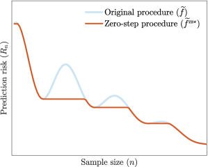
Figure 2: Illustration of risk monotonization.

Suppose $R_{n}$ represents the prediction risk of a given prediction procedure ${\widetilde{f}}$ on a dataset containing $n$ i.i.d. observations. It is desirable that $R_{n}$ as a function of $n\geq 1$ is non-increasing. As described above, this however may not hold for an arbitrary procedure ${\widetilde{f}}$. If we have access to $R_{k}$ for $1\leq k\leq n$, then one could just return the predictor obtained by applying the prediction procedure ${\widetilde{f}}$ on a subset of $k^{\star}_{n}$ i.i.d. observations where $k^{\star}_{n}=\mathop{\mathrm{arg\,min}}\{R_{k}:1\leq k\leq n\}$. This procedure, (denoted by, say) ${\widetilde{f}}^{\mathrm{zs}\star}$, essentially returns a predictor whose risk is the largest non-increasing function that is below the risk of ${\widetilde{f}}$; see Figure 2 for an illustration.

It is trivially true that the risk of the prediction procedure ${\widetilde{f}}^{\mathrm{zs}\star}$ as a function of $n\geq 1$ is non-decreasing and its risk at the sample size $n$ is given by $\min_{k\leq n}R_{k}$. This procedure ${\widetilde{f}}^{\mathrm{zs}\star}$ is, however, not actionable in practice because one seldom has access to the true risk $R_{n}$ of ${\widetilde{f}}$.

The goal of this section is to develop a prediction procedure ${\widehat{f}}^{\mathrm{zs}}$ starting with the base prediction procedure ${\widetilde{f}}$ such that the risk of ${\widehat{f}}^{\mathrm{zs}}$ is the largest non-increasing function that is below the risk of ${\widetilde{f}}$ (asymptotically). We achieve this goal by applying Algorithm 1 with the ingredient predictors being the prediction procedure ${\widetilde{f}}$ applied on the subsets of the original data of varying sample sizes.

Remark 3.1 (Conditional versus unconditional risk).

There are two versions of the prediction risk $R_{n}$ that one can consider: conditional (on the dataset $\mathcal{D}_{n}$) and unconditional/non-stochastic. The conditional risk is not just a function of sample size, but also of the data $\mathcal{D}_{n}$. Hence, the conditional risk $R_{k}$, for $k\leq n$, is ill-defined as just a function of the sample size $k$. Therefore, the motivation above should be considered with respect to a non-stochastic approximation of the conditional risk. See Section 3.3 for a precise definition of a non-stochastic approximation of the conditional risk which respect to which we talk of risk monotonization in the sample size.

3.2 Formal description

Formally, let the original dataset be denoted by $\mathcal{D}_{n}=\{(X_{1},Y_{1}),\dots,(X_{n},Y_{n})\}$. As in Algorithm 1, consider the training and testing datasets $\mathcal{D}_{\mathrm{tr}}$ and $\mathcal{D}_{\mathrm{te}}$, respectively. Note that our choice of $n_{\mathrm{te}}$ as described in Remark 2.13 satisfies $n_{\mathrm{te}}=o(n)$, and hence, the risk of ${\widetilde{f}}$ trained on $\mathcal{D}_{\mathrm{tr}}$ is expected to be asymptotically the same as the risk of ${\widetilde{f}}$ trained on $\mathcal{D}_{n}$.

To achieve the goal described in Section 3.1, one can define the ingredient predictors required in Algorithm 1 as follows: Let $\mathcal{D}_{\mathrm{tr}}^{k}$ denote a subset of $\mathcal{D}_{\mathrm{tr}}$ with $n_{\mathrm{tr}}-k$ observations for $1\leq k\leq n_{\mathrm{tr}}$. For $\Xi_{n}=\{1,2,\dots,n_{\mathrm{tr}}-1\}$ and $\xi\in\Xi_{n}$, define ${\widetilde{f}}^{\xi}(x)={\widetilde{f}}(x;\mathcal{D}_{\mathrm{tr}}^{\xi})$ as the predictor obtained by training ${\widetilde{f}}$ on $\mathcal{D}_{\mathrm{tr}}^{\xi}$. Proposition 2.1 along with Lemmas 2.4 and 2.5 and Lemmas 2.9 and 2.10 can be used to imply that ${\widehat{f}}^{\mathrm{cv}}$ thus obtained has a non-increasing risk as a function of the sample size.

There are two important points to note here:

1. The external randomness of choosing a subset $\mathcal{D}_{\mathrm{tr}}^{\xi}\subseteq\mathcal{D}_{n}$ of size $\xi$. Observe that there are $\binom{n_{\mathrm{tr}}}{\xi}$ different subsets each with $n_{\mathrm{tr}}-\xi$ i.i.d. observations. Asymptotically, the prediction risk of ${\widetilde{f}}$ trained on any of these subsets would be the same. To reduce such external randomness and make use of many different subsets of the same size, we take the ingredient predictor ${\widehat{f}}^{\xi}$ to be:

   $${\widehat{f}}^{\xi}(x)=\frac{1}{M}\sum_{j=1}^{M}{\widetilde{f}}(x;\mathcal{D}_{\mathrm{tr}}^{\xi,j}),$$ (26)

   where $\mathcal{D}_{\mathrm{tr}}^{\xi,j}$, $1\leq j\leq M$ are $M$ sets drawn independently (with replacement) from the collection of $\binom{n_{\mathrm{tr}}}{\xi}$ subsets of $\mathcal{D}_{\mathrm{tr}}$ of size $n_{\mathrm{tr}}-\xi$. With $M=\infty$, ${\widehat{f}}^{\xi}$ becomes the average of ${\widetilde{f}}$ trained on all possible subsets of $\mathcal{D}_{\mathrm{tr}}$ of size $n_{\mathrm{tr}}-\xi$. This choice of $M$ removes any potential external randomness in defining ${\widehat{f}}^{\xi}$. The choice of $M=1$ has the largest amount of external randomness. Based on the theory of $U$-statistics (Serfling,, 2009, Chapter 5), we expect the choice $M=\infty$ to yield a predictor with the smallest variance; see (63). Observe that the expected value ${\widehat{f}}^{\xi}(x)$ remains constant as $M$ changes because the distribution of $\mathcal{D}_{\mathrm{tr}}^{\xi,j}$ remains identical across $j\geq 1$. However, the computation of ${\widehat{f}}^{\xi}$ with $M=\infty$ is infeasible, and hence, we use a finite $M\geq 1$.

2. In the description above, we have $n_{\mathrm{tr}}$ predictors to use in Algorithm 1. Note that the risk of a predictor trained on $m+1$ observations is asymptotically no different from that of a predictor trained on $m$ observations. The same comment holds true for predictors trained on $m+o(m)$ and $m$ observations. For this reason, we can replace $\Xi_{n}=\{1,2,\dots,n_{\mathrm{tr}}-1\}$ with

   $$\Xi_{n}=\left\{1,2,\dots,\left\lceil\frac{n_{\mathrm{tr}}}{\lfloor n^{\nu}\rfloor}-2\right\rceil\right\},\quad\text{ for some }\nu\in(0,1),$$ (27)

   and consider predictors obtained by training ${\widetilde{f}}$ on subsets of sizes $n_{\mathrm{tr}}-\xi\lfloor n^{\nu}\rfloor$ for $\xi\in\Xi_{n}$. This helps in reducing the computational cost of obtaining ${\widehat{f}}^{\mathrm{cv}}$ using Algorithm 1. This further helps in the theoretical properties of ${\widehat{f}}^{\mathrm{cv}}$ in our application of union bound in the results of Section 2.

Taking into account the remarks above, with $\Xi$ as in (27), for $\xi\in\Xi_{n}$, we define ${\widehat{f}}^{\xi}$ as in (26), but with an important change that $\mathcal{D}_{\mathrm{tr}}^{\xi,j}$, $1\leq j\leq M$, now represent randomly drawn subsets of $\mathcal{D}_{\mathrm{tr}}$ of size $n_{\xi}=n_{\mathrm{tr}}-\xi\lfloor n^{\nu}\rfloor$. The ingredient predictors used in Algorithm 1 are given by ${\widehat{f}}^{\xi}$, $\xi\in\Xi_{n}$. We call the resulting predictor obtained from Algorithm 1 as the zero-step predictor based on ${\widetilde{f}}$ and we denote the corresponding prediction procedure to be ${\widehat{f}}^{\mathrm{zs}}$. The zero-step procedure is summarized in Algorithm 2.

Inputs:

• all inputs of Algorithm 1 other than the index set $\Xi$;

• a positive integer $M$.

Output:

• a predictor ${\widehat{f}}^{\mathrm{zs}}$

Procedure:

1. Let $n_{\mathrm{tr}}=n-n_{\mathrm{te}}$. Construct an index set $\Xi_{n}$ per (27).

2. Construct train and test sets $\mathcal{D}_{\mathrm{tr}}$ and $\mathcal{D}_{\mathrm{te}}$ per Step 1 of Algorithm 1.

3. Let $n_{\xi}=n_{\mathrm{tr}}-\xi\lfloor n^{\nu}\rfloor$. For each $\xi\in\Xi_{n}$ and $j=1,\dots,M$, draw random subsets $\mathcal{D}_{\mathrm{tr}}^{\xi,j}$ of size $n_{\xi}$ from $\mathcal{D}_{\mathrm{tr}}$. For each $\xi\in\Xi$, fit predictors ${\widehat{f}}^{\xi}$ per (26) using prediction procedure ${\widetilde{f}}$ and $\{\mathcal{D}_{\mathrm{tr}}^{\xi,j}:1\leq j\leq M\}$.

4. Run Steps 3–5 of Algorithm 1 using index set $\Xi=\Xi_{n}$ and set of predictors $\{{\widehat{f}}^{\xi}$, $\xi\in\Xi\}$.

5. Return ${\widehat{f}}^{\mathrm{zs}}$ as the resulting ${\widehat{f}}^{\mathrm{cv}}$ from Algorithm 1.

Algorithm 2 Zero-step procedure

3.3 Risk behavior of ${\widehat{f}}^{\mathrm{zs}}$

As alluded to before, in order to talk about risk monotonization, one needs to consider a non-stochastic approximation to the conditional risk that depends only on the prediction procedure, the sample size, and properties of the data distribution. The definition below makes this precise.

Definition 3.2 (Deterministic approximation of conditional prediction risk).

For any prediction procedure ${\widetilde{f}}$, we call a map $R^{\mathrm{det}}(\cdot;{\widetilde{f}}):\mathbb{N}\to\mathbb{R}_{\geq 0}$ a deterministic (or non-stochastic) approximation of the conditional risk of ${\widetilde{f}}$ if for all datasets $\mathcal{D}_{m}$ of $m$ i.i.d. random vectors,

$$\frac{|R({\widetilde{f}}(\cdot;\mathcal{D}_{m}))-R^{\mathrm{det}}(m;{\widetilde{f}})|}{R^{\mathrm{det}}(m;{\widetilde{f}})}=o_{p}(1),$$ (28)

as $m\to\infty$. (Recall that $R({\widetilde{f}}(\cdot,\mathcal{D}_{m}))=\int\ell(y;{\widetilde{f}}(x;\mathcal{D}_{m}))\mathrm{d}P(x,y)$.)

It is important to recognize that $R^{\mathrm{det}}(m;{\widehat{f}})$ is only a function of the sample size $m$, the prediction procedure ${\widetilde{f}}$, and the underlying distribution $P$, and not the dataset $\mathcal{D}_{m}$. Note that we do not necessarily require $R^{\mathrm{det}}(m;{\widetilde{f}})$ to be the expected value of $R({\widetilde{f}}(\cdot;\mathcal{D}_{m}))$. Furthermore, a non-asymptotic approximation $R^{\mathrm{det}}(\cdot;{\widetilde{f}})$ of the conditional risk may not be unique.

Remark 3.3 (Relative convergence in Definition 3.2).

In (28), the division by $R^{\mathrm{det}}(m;{\widetilde{f}})$ ensures that the deterministic approximation to the conditional risk of ${\widetilde{f}}(\cdot;\mathcal{D}_{m})$ is non-trivial (i.e., non-zero) even if the conditional risk converges in probability to zero. If the conditional risk is bounded away from zero, asymptotically, then (28) is trivially implied by

$$|R({\widetilde{f}}(\cdot;\mathcal{D}_{m}))-R^{\mathrm{det}}(m;{\widetilde{f}})|=o_{p}(1),$$

as $m\to\infty$. In most settings of overparameterized learning, the conditional prediction risk is asymptotically bounded away from zero (see (36), for example).

Because $|\Xi_{n}|\leq n$, the results of Section 2 imply that with appropriate choices of CEN and $\eta$ in Algorithm 1 we obtain ${\widehat{f}}^{\mathrm{zs}}$ that satisfies the following risk bound:

$$R({\widehat{f}}^{\mathrm{zs}})=\begin{cases}\min_{\xi\in\Xi_{n}}R({\widehat{f}}^{\xi})+O_{p}(1)\sqrt{\log n/n_{\mathrm{te}}}&\text{ if }\widehat{\sigma}_{\Xi}=O_{p}(1)\\ \min_{\xi\in\Xi_{n}}R({\widehat{f}}^{\xi})\big{(}1+O_{p}(1)\sqrt{\log n/n_{\mathrm{te}}}\big{)}&\text{ if }\widehat{\kappa}_{\xi}=O_{p}(1).\end{cases}$$ (29)

Assume now there exists a function $R^{\mathrm{det}}:\mathbb{N}\to\mathbb{R}_{\geq 0}$ such that the following holds:

$$\lim_{n\to\infty}\,\sup_{\xi_{n}\in\Xi_{n}}\,\mathbb{P}\left(\frac{|R({\widetilde{f}}(\cdot;\mathcal{D}_{\mathrm{tr}}^{\xi_{n},j}))-R^{\mathrm{det}}(n_{\xi_{n}};{\widetilde{f}})|}{R^{\mathrm{det}}(n_{\xi_{n}};{\widetilde{f}})}>\epsilon\right)=0\quad\text{for all }\epsilon>0.$$ (DET)

Recall that $\mathcal{D}_{\mathrm{tr}}^{\xi_{n},j}$ for $1\leq j\leq n$ are identically distributed, and hence, ${\widetilde{f}}(\cdot,\mathcal{D}_{\mathrm{tr}}^{\xi_{n},j})$ are also identically distributed predictors. This implies that assuming (DET) for $j=1$ is the same as assuming it for all $1\leq j\leq M$. Note that (DET) is essentially the same as (28), but with a different sequence of sample sizes $\{n_{\xi_{n}}\}_{n\geq 1}$ with $\xi_{n}\in\Xi_{n}$. In accordance with our goal of monotonizing the non-stochastic approximation $R^{\mathrm{det}}(\cdot;{\widetilde{f}})$ of the prediction procedure ${\widetilde{f}}$, we aim to show that the zero-step prediction procedure ${\widehat{f}}^{\mathrm{zs}}$ has its conditional prediction risk approximated by $\min_{\xi\in\Xi_{n}}R^{\mathrm{det}}(n_{\xi};{\widetilde{f}})$. For notational convenience, set

$$R^{\mathrm{det}}_{\nearrow}(n;{\widetilde{f}})~{}:=~{}\min_{\xi\in\Xi_{n}}R^{\mathrm{det}}(n_{\xi};{\widetilde{f}})\quad\text{and}\quad\xi^{\star}_{n}~{}\in~{}\mathop{\mathrm{arg\,min}}_{\xi\in\Xi_{n}}R^{\mathrm{det}}(n_{\xi};{\widetilde{f}}).$$ (30)

Note the notation above is meant to reflect that the index $\xi^{\star}_{n}$ can be chosen to be any element of the minimizing set. If $\Xi_{n}=\{1,\dots,n_{\mathrm{tr}}-1\}$, and $\nu=0$, then $R^{\mathrm{det}}_{\nearrow}(n;{\widetilde{f}})=\min\{R^{\mathrm{det}}(k;{\widetilde{f}}):1\leq k\leq n_{\mathrm{tr}}-1\}$. Although it might be tempting to take $\Xi_{n}=\{1,\dots,n_{\mathrm{tr}}-1\}$ and $\nu=0$, instead of the one in (27), assumption (DET) for all non-stochastic sequences $\{n_{\xi_{n}}\}_{n\geq 1}$ with $\xi_{n}\in\Xi_{n}$ becomes almost certainly unreasonable. To see this, observe that $\xi_{n}=n_{\mathrm{tr}}-1$ belongs to $\Xi_{n}$ for every $n$, and for this choice, $n_{\xi_{n}}=1$. Hence, the predictor ${\widetilde{f}}(\cdot;\mathcal{D}_{\mathrm{tr}}^{\xi,j})$ is computed based on one observation, and cannot satisfy (DET). In the following calculations, however, we only require assumption (DET) for the non-stochastic sequence $\{\xi^{\star}_{n}\}_{n\geq 1}$. If $n_{\xi^{\star}_{n}}$ is known to diverge to $\infty$ and the distribution of the data stays constant, then assumption (DET) is reasonable and is exactly the same as the existence of a deterministic approximation to the conditional risk of ${\widetilde{f}}$ in the sense of Definition 3.2. In this favorable case of $n_{\xi_{n}^{\star}}$ diverging to $\infty$ with $n$, one can take $\Xi_{n}=\{1,\dots,n_{\mathrm{tr}}-1\}$, and $\nu=0$. Note that with $\Xi_{n}$ as defined in (27), $n_{\xi_{n}}\to\infty$ for all $\xi_{n}\in\Xi_{n}$, and thus in particular $n_{\xi_{n}^{\star}}\to\infty$ as $n\to\infty$.

It should be stressed that (DET) is an assumption on the base prediction procedure ${\widetilde{f}}$ and not on the ingredient predictors ${\widehat{f}}^{\xi}$. In general, the risk behavior of ${\widetilde{f}}$ does not necessarily imply that of ${\widehat{f}}^{\xi}$ which is an average of $M$ predictors obtained from ${\widetilde{f}}$. However, the risk of ${\widehat{f}}^{\xi}$ can be bounded in terms of the risk ${\widetilde{f}}$ for loss functions $\ell(\cdot,\cdot)$ that are convex in the second argument. Observe that

$$R({\widehat{f}}^{\xi})~{}=~{}R\left(\frac{1}{M}\sum_{j=1}^{M}{\widetilde{f}}(\cdot;\mathcal{D}_{\mathrm{tr}}^{\xi,j})\right)~{}\leq~{}\frac{1}{M}\sum_{j=1}^{M}R({\widetilde{f}}(\cdot;\mathcal{D}_{\mathrm{tr}}^{\xi,j})).$$ (31)

The inequality (31) follows from Jensen’s inequality. It becomes an equality if $M=1$ without the requirement that the loss function is convex.

Inequality (31) along with the non-stochastic risk approximation (DET) can be used to control $\min_{\xi\in\Xi_{n}}R({\widehat{f}}^{\xi})$ in (29). From (30), we obtain

$$\begin{split}\min_{\xi\in\Xi_{n}}R({\widehat{f}}^{\xi})\overset{(a)}{\leq}\min_{\xi\in\Xi_{n}}\frac{1}{M}\sum_{j=1}^{M}R({\widetilde{f}}(\cdot;\mathcal{D}_{\mathrm{tr}}^{\xi,j}))&\overset{(b)}{\leq}\frac{1}{M}\sum_{j=1}^{M}R({\widetilde{f}}(\cdot;\mathcal{D}_{\mathrm{tr}}^{\xi_{n}^{\star},j}))\\ &=R^{\mathrm{det}}(n_{\xi_{n}^{\star}};{\widetilde{f}})\left(1+\frac{1}{M}\sum_{j=1}^{M}\frac{R({\widetilde{f}}(\cdot,\mathcal{D}_{\mathrm{tr}}^{\xi_{n}^{\star},j}))-R^{\mathrm{det}}(n_{\xi_{n}^{\star}};{\widetilde{f}})}{R^{\mathrm{det}}(n_{\xi_{n}^{\star}};{\widetilde{f}})}\right)\\ &\overset{(c)}{=}\min_{\xi\in\Xi_{n}}R^{\mathrm{det}}(n_{\xi};{\widetilde{f}})(1+o_{p}(1))\\ &=R^{\mathrm{det}}_{\nearrow}(n;{\widetilde{f}})(1+o_{p}(1)).\end{split}$$ (32)

Inequality $(a)$ in (32) follows from using Jensen’s inequality. Inequality $(b)$ follows because $\xi_{n}^{\star}\in\Xi_{n}$. Equality $(c)$ follows for any fixed $M\geq 1$ from the non-stochastic risk approximation (DET); this can be seen from the fact that the sum of a finite number of $o_{p}(1)$ random variables is $o_{p}(1)$.

All the inequalities in (32) can be made equalities for $M=1$, if instead of (DET) we make the stronger assumption that

$$\lim_{n\to\infty}\,\mathbb{P}\left(\sup_{\xi_{n}\in\Xi_{n}}\,\frac{|R({\widetilde{f}}(\cdot;\mathcal{D}_{\mathrm{tr}}^{\xi_{n},j}))-R^{\mathrm{det}}(n_{\xi_{n}};{\widetilde{f}})|}{R^{\mathrm{det}}(n_{\xi_{n}};{\widetilde{f}})}>\epsilon\right)=0\quad\text{for all }\epsilon>0.$$ (DET*)

This is clearly a stronger assumption than required for (32), where we only required such relative convergence for a specific $\xi_{n}^{\star}\in\Xi_{n}$. Under (DET*), we can write

$$\min_{\xi\in\Xi_{n}}\frac{1}{M}\sum_{j=1}^{M}R({\widetilde{f}}(\cdot;\mathcal{D}_{\mathrm{tr}}^{\xi,j})) =\min_{\xi\in\Xi_{n}}R^{\mathrm{det}}(n_{\xi};{\widetilde{f}})\left(1+\frac{1}{M}\sum_{j=1}^{M}\frac{R({\widetilde{f}}(\cdot;\mathcal{D}_{\mathrm{tr}}^{\xi,j}))-R^{\mathrm{det}}(n_{\xi};{\widetilde{f}})}{R^{\mathrm{det}}(n_{\xi};{\widetilde{f}})}\right)$$

$$\lessgtr R^{\mathrm{det}}_{\nearrow}(n;{\widetilde{f}})\left(1\pm\frac{1}{M}\sum_{j=1}^{M}\sup_{\xi\in\Xi_{n}}\left|\frac{R({\widetilde{f}}(\cdot;\mathcal{D}_{\mathrm{tr}}^{\xi,j}))-R^{\mathrm{det}}(n_{\xi};{\widetilde{f}})}{R^{\mathrm{det}}(n_{\xi};{\widetilde{f}})}\right|\right)$$

$$=R^{\mathrm{det}}_{\nearrow}(n;{\widetilde{f}})(1+o_{p}(1)).$$

We now conclude that for $M=1$,

$$\min_{\xi\in\Xi_{n}}R({\widehat{f}}^{\xi})=\min_{\xi\in\Xi_{n}}R({\widetilde{f}}(\cdot;\mathcal{D}_{\mathrm{tr}}^{\xi,1}))=R^{\mathrm{det}}_{\nearrow}(n;{\widetilde{f}})(1+o_{p}(1)).$$ (33)

This proves that all the inequalities in (32) can be made equalities for $M=1$ under the stronger assumption (DET*). Combined with (29), this implies that

$$\begin{split}R({\widehat{f}}^{\mathrm{zs}})&=\begin{cases}R^{\mathrm{det}}_{\nearrow}(n;{\widetilde{f}})(1+o_{p}(1))+O_{p}(1)\sqrt{\log n/n_{\mathrm{te}}}&\text{ if }\widehat{\sigma}_{\Xi}=O_{p}(1)\\ R^{\mathrm{det}}_{\nearrow}(n;{\widetilde{f}})(1+o_{p}(1))&\text{ if }\widehat{\kappa}_{\Xi}=O_{p}(1)\end{cases}\\ &=R^{\mathrm{det}}_{\nearrow}(n;{\widetilde{f}})\begin{cases}1+o_{p}(1)+\sqrt{\log n/n_{\mathrm{te}}}/R^{\mathrm{det}}_{\nearrow}(n;{\widetilde{f}})&\text{ if }\widehat{\sigma}_{\Xi}=O_{p}(1)\\ 1+o_{p}(1)&\text{ if }\widehat{\kappa}_{\Xi}=O_{p}(1).\end{cases}\end{split}$$ (34)

As mentioned before, assumption (DET*) is significantly stronger than (DET). In the absence of (DET*), inequality (32) combined with (29) implies that (34) holds with inequalities instead of equalities. For simplicity, denote:

1. $\widehat{\sigma}_{\Xi}=O_{p}(1)$ and $R^{\mathrm{det}}_{\nearrow}(n;{\widetilde{f}})\sqrt{n_{\mathrm{te}}/\log n}\to\infty$.

2. $\widehat{\kappa}_{\Xi}=O_{p}(1)$.

Hence, we have proved the following result:

Theorem 3.4 (Monotonization by zero-step procedure).

For $M=1$, if assumption (DET*) and either (O1) or (O2) hold true, then $R^{\mathrm{det}}_{\nearrow}(\cdot;{\widetilde{f}})$ is a deterministic approximation of the prediction procedure ${\widehat{f}}^{\mathrm{zs}}$, i.e.,

$$\frac{|R({\widehat{f}}^{\mathrm{zs}})-R^{\mathrm{det}}_{\nearrow}(n;{\widetilde{f}})|}{R^{\mathrm{det}}_{\nearrow}(n;{\widetilde{f}})}=o_{p}(1).$$

For $M\geq 1$, if $\ell(\cdot,\cdot)$ is convex in the second argument, assumption (DET), and either (O1) or (O2) hold true, then

$$\frac{(R({\widehat{f}}^{\mathrm{zs}})-R^{\mathrm{det}}_{\nearrow}(n;{\widetilde{f}}))_{+}}{R^{\mathrm{det}}_{\nearrow}(n;{\widetilde{f}})}=o_{p}(1).$$

Remark 3.5 (Choice of $\Xi_{n}$).

All the calculations presented in this section hold for any set $\Xi_{n}$ with $|\Xi_{n}|\leq n$. As long as either (DET) (for $\xi_{n}=\xi_{n}^{\star}$ in (30)) or (DET*) holds true, then one can use $\Xi_{n}=\{1,2,\ldots,n_{\mathrm{tr}}-1\}$ and $\nu=0$. For this choice, $R^{\mathrm{det}}_{\nearrow}(\cdot;\widehat{f})$ is the monotonized risk as illustrated in Figure 2. With the choice of $\Xi_{n}$ mentioned in (27), $R^{\mathrm{det}}_{\nearrow}(\cdot;\widehat{f})$ is not a complete monotonization but it serves as an approximate monotone risk.

Remark 3.6 (Exact risk ${\widehat{f}}^{\mathrm{zs}}$).

For $M=1$ (under (DET*)), Theorem 3.4 essentially implies that the risk of the zero-step procedure closely tracks the monotonized deterministic approximation to the conditional prediction risk of ${\widetilde{f}}$ trained on $\mathcal{D}_{\mathrm{tr}}$. For $M\geq 1$ (under (DET)), Theorem 3.4 does not imply the risk of the zero-step predictor is monotonic or even that that a non-stochastic approximation of the risk exists in the sense of Definition 3.2. However, our simulations in limited settings presented in Section 3.4 suggest that the risk of the zero-step prediction procedure is monotone even for $M\geq 1$.

Remark 3.7 (Verification of assumptions in Theorem 3.4).

The bound on $\widehat{\sigma}_{\Xi}$ and $\widehat{\kappa}_{\Xi}$ in Assumptions (O1) and (O2) can be verified for some common loss functions and predictors as discussed in Section 2.3. The verification of assumption (DET) or (DET*) is very much tied to the exact prediction procedure. We verify (DET) in a specific setting in Section 3.3.1.

3.3.1 Risk behavior of ${\widehat{f}}^{\mathrm{zs}}$ under proportional asymptotics

In the discussion leading up to Theorem 3.4, we have not made a specific reference to the growth or non-growth of the dimension of the features. Technically, Theorem 3.4 does allow for the dimension $p$ of the features to change with the sample size $n$, i.e., one can have $p=p_{n}$.

Risk monotonization is an interesting phenomenon to study in light of the double (or multiple) descent results in the overparameterized setting where $p_{n}/n\to\gamma$ as $n\to\infty$. In our previous discussion of non-stochastic approximation of the conditional prediction risk, we did not stress the dependence on the dimension of features. In the following, we consider the implications of Theorem 3.4 in the context of overparameterized learning and hence consider the following setting.

Recall that the original dataset $\mathcal{D}_{n}$ consists of $n$ i.i.d. observations $(X_{i},Y_{i})\in\mathbb{R}^{p}\times\mathbb{R}$, $1\leq i\leq n$ from distribution $P$. In the following as we allow the dimension $p$ of the features to change with the sample size $n$ and assume that $p=p_{n}$ satisfies

1. $p_{n}/n\to\gamma\in(0,\infty)$ as $n\to\infty$.

The above asymptotic regime, which is standard in random matrix theory (Bai and Silverstein,, 2010), is used in the overparameterized learning literature, where it has been referred to as proportional asymptotics. (see e.g., Dobriban and Wager, (2018); Hastie et al., (2019); Mei and Montanari, (2019); Bartlett et al., (2021)). Note that under assumption (PA($\gamma$)) the underlying distribution $P$ of the observations in $\mathcal{D}_{n}$ should be indexed by the sample size $n$. We suppress this dependence for convenience. Under the proportional asymptotics regime for commonly studied prediction procedures, a deterministic approximation to the conditional prediction risk of a subset $\mathcal{D}_{m}\subseteq\mathcal{D}_{n}$ depends not on $m$ but on $p_{n}/m$, among other properties of the distribution $P$. For this reason, in any discussion of the deterministic approximation of the conditional prediction risk, we write $R^{\mathrm{det}}(p_{n}/m;{\widetilde{f}})$ instead of $R^{\mathrm{det}}(m;{\widetilde{f}})$. Now the goal of this subsection is to derive the deterministic approximation of the conditional risk of the zero-step predictor under (PA($\gamma$)).

Recall that from the crucial calculation in (32) leading to the risk of zero-step predictor, we require

$$\frac{R({\widetilde{f}}(\cdot,\mathcal{D}_{\mathrm{tr}}^{\xi_{n}^{\star},j}))-R^{\mathrm{det}}(n_{\xi_{n}^{\star}};{\widetilde{f}})}{R^{\mathrm{det}}(n_{\xi_{n}^{\star}};{\widetilde{f}})}=o_{p}(1),$$ (35)

with $\xi^{\star}_{n}$ defined as in (30). Except for (35), all the remaining steps in (32) hold true even in the overparameterized setting. In the following, we will provide simple sufficient condition for verification of (35) under (PA($\gamma$)). As mentioned above, the deterministic risk under (PA($\gamma$)) often depends not only on the sample size alone, but also on the ratio of the number of features to the sample size. Therefore, we find it helpful to rewrite (35) as

$$\frac{R({\widetilde{f}}(\cdot;\mathcal{D}_{\mathrm{tr}}^{\xi_{n}^{\star},j}))-R^{\mathrm{det}}(p_{n}/n_{\xi_{n}^{\star}};{\widetilde{f}})}{R^{\mathrm{det}}(p_{n}/n_{\xi_{n}^{\star}};{\widetilde{f}})}=o_{p}(1),\quad\text{where}\quad\xi_{n}^{\star}\in\mathop{\mathrm{arg\,min}}_{\xi\in\Xi_{n}}R^{\mathrm{det}}(p_{n}/n_{\xi};{\widetilde{f}}).$$ (DETPA-0)

Note that assumption (PA($\gamma$)) does not imply that $p_{n}/n_{\xi_{n}^{\star}}$ converges to a fixed limit as $n\to\infty$.

Under assumption (DETPA-0), Theorem 3.4 readily implies the risk behavior of ${\widehat{f}}^{\mathrm{zs}}$. However, the possibility that $p_{n}/n_{\xi_{n}^{\star}}$ does not converge to a fixed limit necessitates a closer examination of assumption (DETPA-0). We provide a two-fold reduction of assumption (DETPA-0). Firstly, it suffices to verify that the absolute difference between $R({\widetilde{f}}(\cdot;\mathcal{D}_{\mathrm{tr}}^{\xi_{n}^{\star},j}))$ and $R^{\mathrm{det}}(p_{n}/n_{\xi_{n}^{\star}};{\widetilde{f}})$ converges to $0$ when $R^{\mathrm{det}}(\cdot;{\widetilde{f}})$ is uniformly bounded away from $0$. This is a reasonable assumption in practice because several loss functions under mild conditions on the response have risk lower bounded by the unavoidable error which is strictly positive. For example, assuming the loss $\ell$ is the squared loss and that $\mathbb{E}[(Y_{0}-\mathbb{E}[Y_{0}\mid X_{0}])^{2}]>0$, we have for any prediction procedure $\widetilde{f}$ and any training dataset $\mathcal{D}_{m}$ containing $m$ observation,

$$R(\widetilde{f}(\cdot;\mathcal{D}_{m}))~{}=~{}\mathbb{E}[(Y_{0}-\widetilde{f}(X_{0};\mathcal{D}_{m}))^{2}\big{|}\mathcal{D}_{m}]~{}\geq~{}\mathbb{E}[(Y_{0}-\mathbb{E}[Y_{0}|X_{0}])^{2}]>0.$$ (36)

Hence, in this case, if there exists a deterministic function $R^{\mathrm{det}}:(0,\infty]\to[0,\infty]$ such that under (PA($\gamma$)), as $n\to\infty$,

$$R({\widetilde{f}}(\cdot;\mathcal{D}_{\mathrm{tr}}^{\xi_{n}^{\star},j}))-R^{\mathrm{det}}(p_{n}/n_{\xi_{n}^{\star}};{\widetilde{f}})=o_{p}(1),\quad\text{where}\quad\xi_{n}^{\star}\in\mathop{\mathrm{arg\,min}}_{\xi\in\Xi_{n}}R^{\mathrm{det}}(p_{n}/n_{\xi};{\widetilde{f}}),$$ (37)

then (DETPA-0) is satisfied. Secondly, the following lemma shows that under (PA($\gamma$)), (37) is satisfied if there exists a deterministic approximation for the conditional risk with datasets having a converging aspect ratio (i.e., datasets for which the ratio of the number of features to the sample size converges to a constant).

For any $\gamma>0$, define

$$\mathcal{M}_{\gamma}^{\mathrm{zs}}~{}:=~{}\mathop{\mathrm{arg\,min}}_{\zeta:\zeta\geq\gamma}R^{\mathrm{det}}(\zeta;{\widetilde{f}}).$$

Lemma 3.8 (Reduction of (DETPA-0)).

Let $\mathcal{D}_{k_{m}}$ be a dataset with $k_{m}$ observations and $p_{m}$ features. Consider a prediction procedure ${\widetilde{f}}$ trained on $\mathcal{D}_{k_{m}}$. Assume the loss function $\ell$ is such that $R({\widetilde{f}}(\cdot;\mathcal{D}_{k_{m}}))$ is uniformly bounded from below by $0$. Let $\gamma>0$ be a real number. Suppose there exists a proper, lower semicontinuous function $R^{\mathrm{det}}(\cdot;{\widetilde{f}}):[\gamma,\infty]\to[0,\infty]$ such that

$$R({\widetilde{f}}(\cdot;\mathcal{D}_{k_{m}}))~{}\xrightarrow{\text{p}}~{}R^{\mathrm{det}}(\phi;{\widetilde{f}}),$$ (DETPAR-0)

as $k_{m},p_{m}\to\infty$ and $p_{m}/k_{m}\to\phi\in\mathcal{M}_{\gamma}^{\mathrm{zs}}$. Further suppose that $R^{\mathrm{det}}(\cdot;{\widetilde{f}})$ is continuous on the set $\mathcal{M}_{\gamma}^{\mathrm{zs}}$. Then, (DETPA-0) is satisfied.

We prove Lemma 3.8 using the real analysis fact that a sequence $\{a_{n}\}_{n\geq 1}$ converges to $0$ if and only if for any subsequence $\{a_{n_{k}}\}_{k\geq 1}$, there exists a further subsequence $\{a_{n_{k_{l}}}\}_{l\geq 1}$ that converges to $0$ (see, for example, Problem 12 of Royden, (1988); also see Lemma S.6.3 for a self-contained proof). We apply this fact to the sequence

$$a_{n}(\epsilon)=\mathbb{P}\left(\left|R({\widetilde{f}}(\cdot;\mathcal{D}_{\mathrm{tr}}^{\xi_{n}^{\star},j}))-R^{\mathrm{det}}(p_{n}/n_{\xi_{n}^{\star}};{\widetilde{f}})\right|\geq\epsilon\right),$$

for every $\epsilon>0$. A crucial component in applying this technique is to first produce a subsequence $\{n_{k_{l}}\}_{l\geq 1}$ such that $p_{n_{k_{l}}}/n_{\xi^{\star}_{n_{k_{l}}}}$ converges to a point in $\mathop{\mathrm{arg\,min}}_{\zeta\in[\gamma,\infty]}R^{\mathrm{det}}(\zeta;{\widetilde{f}})$. A few remarks on the assumptions of Lemma 3.8 are in order.

• In most cases, the set of minimizers of $R^{\mathrm{det}}(\cdot;{\widetilde{f}})$ is a singleton set. For such a scenario, Lemma 3.8 only requires the deterministic approximation of the conditional prediction risk for a single limiting aspect ratio (i.e., (DETPAR-0) is only required for a single $\phi$). Several commonly studied predictors satisfy (DETPAR-0) as discussed below.

• Assuming lower semicontinuity of $R^{\mathrm{det}}(\cdot;{\widetilde{f}})$ is a mild assumption. In particular, it does not preclude the possibility that $R^{\mathrm{det}}$ diverges to $\infty$ at several values in the domain as shown in Proposition 3.9. Such risk diverging behavior is a common occurrence for several popular predictors in overparameterized learning, for example, MN2LS, MN1LS, etc. The requirement of the lower semicontinuity stems from the goal of monotonizing $R^{\mathrm{det}}$ from below.

Proposition 3.9 (Verifying lower semicontinuity for diverging risk profiles).

Suppose $h:[a,c]\to\mathbb{R}$ is continuous on $[a,b)\cup(b,c]$ and $\lim_{x\to b^{-}}h(x)=\lim_{x\to b^{+}}h(x)=\infty$. Then, $h$ is lower semicontinuous on $[a,c]$.

• Proposition 3.9 implies that if $R^{\mathrm{det}}$ is continuous on a set except for a point where it diverges to $\infty$, then $R^{\mathrm{det}}$ is lower semicontinuous on that set. In this sense, Proposition 3.9 relates the lower semicontinuity assumption of Lemma 3.8 to the continuity assumption of the lemma.

• Continuity assumption on $R^{\mathrm{det}}(\cdot;{\widetilde{f}})$ at the argmin set $\mathop{\mathrm{arg\,min}}_{\zeta\in[\gamma,\infty]}R^{\mathrm{det}}(\zeta;{\widetilde{f}})$ is also mild. Proposition 3.10 below shows that (DETPAR-0) holding for $\phi$ in any open set $\mathcal{I}$ implies continuity of $R^{\mathrm{det}}$ on $\mathcal{I}$. In particular, this implies continuity on the sets of the type $\mathcal{I}=(a,\infty]$. If the set of minimizers of $R^{\mathrm{det}}$ is a singleton set, then (DETPAR-0) itself does not suffice to guarantee the continuity of $R^{\mathrm{det}}$ at the minimizer. Proposition 3.10 in such a case requires verifying (DETPAR-0) on an open interval containing the minimizer.

Proposition 3.10 (Certifying continuity from continuous convergence).

Let $\mathcal{D}_{k_{m}}$ be a dataset with $k_{m}$ observations and $p_{m}$ features, and consider a prediction procedure ${\widetilde{f}}$ trained on $\mathcal{D}_{k_{m}}$. Let $\mathcal{I}$ be an open set in $(0,\infty)$. Suppose there exists a function $R^{\mathrm{det}}:(0,\infty]\to[0,\infty]$ such that

$$R({\widetilde{f}}(\cdot;\mathcal{D}_{k_{m}}))~{}\xrightarrow{\text{p}}~{}R^{\mathrm{det}}(\phi;{\widetilde{f}})$$ (38)

as $k_{m},p_{m}\to\infty$ and $p_{m}/k_{m}\to\phi\in\mathcal{I}$. Then, $R^{\mathrm{det}}(\cdot;{\widetilde{f}})$ is continuous on $\mathcal{I}$.

Combining the results and the discussion above, the verification of (DETPA-0) under (PA($\gamma$)) can proceed with the following two-step program.

1. For $\phi$ such that $R^{\mathrm{det}}(\phi;{\widetilde{f}})<\infty$, verify that for all datasets $\mathcal{D}_{k_{m}}$ with limiting aspect ratio $\phi$, $R({\widetilde{f}}(\cdot;\mathcal{D}_{k_{m}}))\xrightarrow{\text{p}}R^{\mathrm{det}}(\phi;{\widetilde{f}})$.

2. Whenever $R^{\mathrm{det}}(\phi;{\widetilde{f}})=\infty$,

   $$\lim_{\phi^{\prime}\to\phi^{-}}R^{\mathrm{det}}(\phi^{\prime};{\widetilde{f}})=\lim_{\phi^{\prime}\to\phi^{+}}R^{\mathrm{det}}(\phi^{\prime};{\widetilde{f}})=\infty.$$

The continuity of $R^{\mathrm{det}}$ at points where it is finite follows from (PRG-0-C1) via Proposition 3.10. This kind of convergence is verified in the literature for several commonly used prediction procedures, such as ridge regression and MN2LS (Hastie et al.,, 2019), lasso and MN1LS (Li and Wei,, 2021), etc; see Remark 3.16 for more details. This combined with (PRG-0-C2) via Proposition 3.9 implies lower semicontinuity of $R^{\mathrm{det}}$ on $[\gamma,\infty]$. If there is more than one $\phi$ at which $R^{\mathrm{det}}$ is $\infty$, then Proposition 3.9 should be applied separately by splitting the domain to only contain one point of divergence. A more general result of this flavour can be found in Proposition 4.2 in Section 4.3.1.

We will follow these steps to verify (DETPA-0) for the ridge and lasso prediction procedures in Section 3.3.2. But first we will complete the derivation of the deterministic approximation to the conditional risk of ${\widehat{f}}^{\mathrm{zs}}$ under (DETPA-0) following (32). Lemma 3.8 combined with Theorem 3.4 proves that the zero-step prediction procedure approximately monotonizes the risk of the base prediction procedure ${\widetilde{f}}$ as shown in the following result:

Theorem 3.11 (Asymptotic risk profile of zero-step predictor).

For any prediction procedure ${\widetilde{f}}$, suppose (PA($\gamma$)), either (O1) or (O2), and the assumptions of Lemma 3.8 hold true. In addition, if the loss function is convex in the second argument, then for any $M\geq 1$,

$$\left(R({\widehat{f}}^{\mathrm{zs}};\mathcal{D}_{n})-\min_{\zeta\geq\gamma}R^{\mathrm{det}}(\zeta;{\widetilde{f}})\right)_{+}=o_{p}(1).$$

Remark 3.12 (Monotonicity in the limiting aspect ratio and improvement over base procedure).

If we replace assumption (DETPA-0) with the stronger version

$$\sup_{\xi\in\Xi_{n}}\frac{|R({\widetilde{f}}(\cdot;\mathcal{D}_{\mathrm{tr}}^{\xi,j}))-R^{\mathrm{det}}(p_{n}/n_{\xi};{\widetilde{f}})|}{R^{\mathrm{det}}(p_{n}/n_{\xi};{\widetilde{f}})}=o_{p}(1),$$ (DETPA-0*)

as $n\to\infty$, then for $M=1$, the conclusion of Theorem 3.11 can be strengthened to

$$\left|R({\widehat{f}}^{\mathrm{zs}};\mathcal{D}_{n})-\min_{\zeta\geq\gamma}R^{\mathrm{det}}(\zeta;{\widetilde{f}})\right|=o_{p}(1).$$ (39)

This implies that the risk of the zero-step procedure is monotonically non-decreasing in $\gamma$. Under the assumptions of Theorem 3.11, one can only conclude that the risk of zero-step procedure is asymptotically bounded above by a monotonically non-decreasing function in $\gamma$ in general. It is trivially true that $\min_{\zeta\leq\gamma}R^{\mathrm{det}}(\zeta;{\widetilde{f}})\leq R^{\mathrm{det}}(\gamma;{\widetilde{f}})$. Hence, the asymptotic risk of zero-step procedure is no worse than that of the base procedure.

Remark 3.13 (Finiteness of the risk of ${\widehat{f}}^{\mathrm{zs}}$).

Predictors such the MN2LS or MN1LS undergo divergence in the prediction risk. The zero-step prediction procedure does not have such a divergence in the risk under general regularity conditions. In particular, as long as $\mathbb{E}[\ell(y,0)]<\infty$, then the risk of ${\widehat{f}}^{\mathrm{zs}}$ is asymptotically bounded by $\mathbb{E}[\ell(y,0)]$. Observe that $\mathbb{E}[\ell(y,0)]$ is the risk of the null predictor which always returns $0$ as its prediction. By including the zero predictor in Algorithm 1, the risk of ${\widehat{f}}^{\mathrm{zs}}$ will always be asymptotically bounded by this null risk.

3.3.2 Verifying deterministic profile assumption (DETPAR-0)

In the following, we will restrict ourselves to the case of linear predictors and squared error loss, and verify assumption (DETPAR-0) for MN2LS and MN1LS base procedures.

Suppose $\mathcal{D}_{k_{m}}=\{(X_{i},Y_{i})\in\mathbb{R}^{p_{m}}\times\mathbb{R}:1\leq i\leq k_{m}\}$. Recall the MN2LS and MN1LS predictor procedures defined in Examples 2.25 and 2.26. It is now well-known that the MN2LS and MN1LS prediction procedures has a non-monotone risk as a function of sample size $n$ (Nakkiran et al.,, 2020; Hastie et al.,, 2019; Li and Wei,, 2021). The following two results verify assumption (DETPAR-0) for these two procedures under some regularity conditions stated in Hastie et al., (2019); Li and Wei, (2021).

Proposition 3.14 (Verification of (DETPAR-0) for MN2LS procedure).

Assume the setting of Theorem 3 of Hastie et al., (2019). Then, there exists a function $R^{\mathrm{det}}(\cdot;{\widetilde{f}}_{\mathrm{mn2}}):(0,\infty]\to[0,\infty]$ such that (PRG-0-C1) holds for all $\phi\neq 1$ and (PRG-0-C2) holds for $\phi=1$.

Proposition 3.15 (Verification of (DETPAR-0) for MN1LS procedure).

Assume the setting of Theorem 2 of Li and Wei, (2021). Then, there exists a function $R^{\mathrm{det}}(\cdot;{\widetilde{f}}_{\mathrm{mn1}}):(0,\infty]\to[0,\infty]$ such that (PRG-0-C1) holds for all $\phi\neq 1$ and (PRG-0-C2) holds for $\phi=1$.

Remark 3.16 (Extending Propositions 3.14 and 3.15 to other predictors).

Theorem 3 of Hastie et al., (2019) only provides the asymptotic behavior of the prediction risk computed conditional only on $\{X_{i},1\leq i\leq k_{m}\}$. The proof in Section S.3 of Proposition 3.14 extends the calculations of of Hastie et al., (2019) for prediction risk conditional on $\mathcal{D}_{k_{m}}$. These calculations can be further extended in a straightforward manner to cover the case of $\lambda>0$, i.e., the ridge regression procedure. See Proposition 3.14 for more details. Similar comments apply to Proposition 3.15 where the proposition can be easily extended to cover the case of $\lambda>0$, i.e., the lasso prediction procedure.

Additionally, most results in the literature under (PA($\gamma$)) derive the risk behavior as $p_{m}/k_{m}\to\phi<\infty$. Propositions 3.14 and 3.15 also extend the existing results to the case when $p_{m}/k_{m}\to\infty$ as $m\to\infty$.

We present Propositions 3.14 and 3.15 as example results to show the verification of our assumptions follow rather easily from the existing asymptotic profile results in the literature. In the proportional asymptotic regime, the risk profiles have been characterized for various other prediction procedures including, high dimensional robust $M$-estimator (Karoui,, 2013, 2018; Donoho and Montanari,, 2016), the Lasso estimator (Miolane and Montanari,, 2021; Celentano et al.,, 2020), and various classification procedures (Montanari et al.,, 2019; Liang and Sur,, 2020; Sur et al.,, 2019). Our results can be suitably extended to verify (DETPA-0) for these other predictors. Note that for our results, we only need to know that the asymptotic risk exists, which can potentially hold true under weaker assumptions.

3.4 Numerical illustrations

In this section, we provide numerical illustration of the risk monotonization of zero-step prediction procedure in the overparameterized setting, when the base prediction procedures are minimum $\ell_{2}$-norm least squares (MN2LS) and minimum $\ell_{1}$-norm least squares (MN1LS). In order to illustrate risk monotonization as in Theorem 3.11, we need to show the risk behavior of ${\widehat{f}}^{\mathrm{zs}}$ at different aspect ratios. We use the following simulation setups for the two predictors.

Minimum $\ell_{2}$-norm least squares (MN2LS).

We fix $n=1000$ and vary the dimension $p$ of the features from $100$ to $10000$ (for a total of $20$ values of $\gamma=p/n$ logarithmically spaced between $0.1$ to $10$). This will show the risk behavior of zero-step procedure for aspect ratios between $0.1$ to $10$. For every pair of sample size $n=1000$ and dimension $p$, we generate $100$ independent datasets each with $n$ i.i.d. observations from the linear model $Y_{i}=X_{i}^{\top}\beta_{0}+\varepsilon_{i}$, where $X_{i}\sim\mathcal{N}(0_{p},I_{p})$, $\beta_{0}\sim\mathcal{N}(0_{p},\rho^{2}/pI_{p})$ and $\varepsilon_{i}\sim\mathcal{N}(0,\sigma^{2})$ drawn independently of $X_{i}$. The model represents a dense signal regime with average signal energy $\rho^{2}$. We define the signal-to-noise ratio (SNR) to be $\rho^{2}/\sigma^{2}$. On each dataset, we apply the MN2LS baseline procedure as well as the zero-step procedure.

In each run, we additionally generate independent test datasets each with $10000$ i.i.d. observations from the same $p+1$ dimensional distribution described above in order to approximate the true risk of the zero-step and the base prediction procedure. Figure 3 shows the risks of the baseline MN2LS procedure and the zero-step prediction procedure for high (left, SNR = 4) and low (right, SNR = 1) SNR regimes; we take $\sigma^{2}=1$ and $\rho^{2}$=SNR. We also present the null risk ($\rho^{2}+\sigma^{2}$), i.e., the risk of the zero predictor as a baseline in both the plots. We observe from the figure that the risk of the zero-step procedure for every $M\geq 1$ is non-decreasing in $\gamma$. Theorem 3.11 implies that the risk of the zero-step prediction procedure for every $M\geq 1$ is asymptotically bounded by the risk of the base prediction procedure at each aspect ratio $(\gamma)$. Although this is somewhat evident from Figure 3, it is not satisfied for all $\gamma$, especially for $M=1$. This primarily stems from the smaller sample size at hand and the fact that we are comparing MN2LS trained on full data ($n=1000$) to the zero-step predictor computed on the train data $(n_{\mathrm{tr}}=900)$. With an increased sample size (to say, $n=2500$), this finite-sample discrepancy vanishes.

Figure 3 shows that the zero-step procedure with $M=1$ attains risk monotonization in a precise sense that its risk is the largest non-increasing function (of $\gamma$) below the risk of the MN2LS predictor. For $M>1$, our results do not characterize the risk of zero-step predictor, but Figure 3 shows that averaging has a significant effect in further reducing the risk. As mentioned before, this is expected from the theory of $U$-statistics as $U$-statistics are UMVUE’s of their expectations (see, e.g., Chapter 5 of Serfling, (2009)). All these comments hold for both low and high SNR alike.

Note that the base predictor has unbounded risk near $\gamma=1$. The risk of the zero-step procedure, on the other hand, is always bounded for all $M\geq 1$ and all $\gamma$. In this sense, the zero-step procedure can also be used as a general procedure for mitigating the surprising descent behavior in the prediction risk.

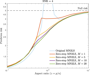
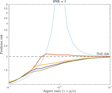
Figure 3: Illustration of the zero-step prediction procedure with MN2LS as the base predictor with varying $M$. The left panel shows a high SNR regime (SNR = 4), while the right panel shows a low SNR regime (SNR = 1). Here, $n=1000$, $n_{\mathrm{tr}}=900$, $n_{\mathrm{te}}=100$, $n^{\nu}=50$. The features are drawn from an isotropic Gaussian distribution, the response follows a linear model. The figure show averaged risk over 100 dataset repetitions.

Minimum $\ell_{1}$-norm least squares (MN1LS).

We fix $n=500$ and vary the dimension $p$ of the features from $50$ to $50000$ (for a total of $30$ values of $\gamma=p/n$ logarithmically spaced between 0.1 to 100). This will show risk behavior of zero-step procedure for aspect ratios between 0.1 and 100. For every pair of sample size $n=500$ and dimension $p$, we generate $250$ independent dataset each with $n$ i.i.d. observations from the linear model $Y_{i}=X_{i}^{\top}\beta_{0}+\varepsilon_{i}$, where $X_{i}\in\mathcal{N}(0_{p},I_{p})$, $\beta_{0}$ has coordinates generated i.i.d. from the distribution $B\delta_{r/\sqrt{p\pi}}+(1-B)\delta_{0}$, where $B\sim\textrm{Bernoulli}(\pi=0.005)$ and $\varepsilon_{i}\sim\mathcal{N}(0,\sigma^{2})$ is independent of $X_{i}$. The model represents a sparse signal regime (with linear sparsity level $\pi$) with average signal energy $\rho^{2}$. We again define SNR to be $\rho^{2}/\sigma^{2}$. On each dataset, we apply MN1LS baseline procedure as well as the zero-step procedure.

In each run, we additionally generate independent test datasets each with $10000$ i.i.d. observations from the same $p+1$ dimensional distribution described above in order to approximate the true risk of the zero-step and the base prediction procedure. Figure 4 shows the risks of the baseline MN1LS procedure and the zero-step procedure for high (left, SNR = 4) and low (right, SNR = 1) SNR regimes. We take $\sigma^{2}=1$ and $\rho^{2}$=SNR. We also present the null risk ($\rho^{2}+\sigma^{2}$), i.e., the risk of the zero predictor as a baseline in both the plots. We again observe that the risk of the zero-step procedure for every $M\geq 1$ is non-decreasing in $\gamma$.

Similar to Figure 3, we observe in Figure 4 that the zero-step procedure with $M=1$ attains precise risk monotonization while zero-step with $M>1$ improves significantly upon the $M=1$ when $\gamma$ is near one. All these comments hold for both low and high SNR alike.

As with Figure 3, note that the base predictor MN2LS has unbounded risk near $\gamma=1$ in Figure 4. The risk of the zero-step procedure, on the other hand, is always bounded for all $M\geq 1$ and all $\gamma$.

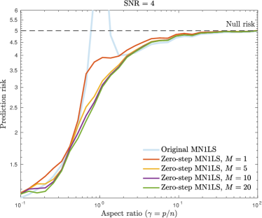
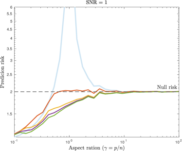
Figure 4: Illustration of the zero-step prediction procedure with MN1LS as the base predictor with varying $M$. The left panel shows a high SNR regime (SNR = 4), while the right panel shows a low SNR regime (SNR = 1). Here, $n=500$, $n_{\mathrm{tr}}=420$, $n_{\mathrm{te}}=80$, $n^{\nu}=42$. The features are drawn from an isotropic Gaussian distribution, the response follows a linear model with sparse signal (sparsity level = 0.005). The risks are averaged over 250 dataset repetitions.

4 Application 2: One-step prediction procedure

4.1 Motivation

The zero-step procedure introduced in Section 3 provides the desired asymptotic monotonization of the conditional prediction risk under certain regularity conditions. It takes advantage of the fact that we can train our predictors on a smaller subset of the data when it is appropriate. In addition, it uses repeated sampling and averaging in order to remove the external randomness in the choice of the subset.

In this section, we introduce a variant of the zero-step procedure motivated by the classical statistical idea of one-step estimation (see, e.g., Section 5.7 of Van der Vaart,, 2000). In the simplest case of linear regression where the feature dimension is fixed, the idea of one-step estimation is that we can start with an arbitrary linear predictor and add to it an adjustment computed based on the residuals of the initial linear predictor. More precisely, starting with any initial estimator ${\widetilde{\beta}}^{\mathrm{init}}$ and the associated linear predictor ${\widetilde{f}}(x)=x^{\top}{\widetilde{\beta}}^{\mathrm{init}}$, we have

$$\underbrace{\vphantom{\left(\frac{1}{n}\sum_{i=1}^{n}X_{i}X_{i}^{\top}\right)^{-1}}X^{\top}{\widetilde{\beta}}^{\mathrm{init}}}_{\text{initial predictor}}+~{}\underbrace{X^{\top}\left(\frac{1}{n}\sum_{i=1}^{n}X_{i}X_{i}^{\top}\right)^{-1}\left(\frac{1}{n}\sum_{i=1}^{n}X_{i}(Y_{i}-X_{i}^{\top}{\widetilde{\beta}}^{\mathrm{init}})\right)}_{\text{one-step adjustment}}=X^{\top}{\widetilde{\beta}}^{\mathrm{ols}},$$ (40)

where the final resulting predictor corresponds to the ordinary least squares (OLS) estimator ${\widetilde{\beta}}^{\mathrm{ols}}$ that enjoys $n^{-1/2}$ rate and risk optimality under a well-specified linear model.

This idea of one-step estimation is not specific to ordinary least squares. It can be generalized to other estimators that are solutions to estimating equation $\Psi_{n}(\beta)=0$ where $\Psi_{n}:\mathbb{R}^{p}\to\mathbb{R}^{p}$. The general idea is to solve a linear approximation to the estimating equation, i.e., given an initial estimator ${\widetilde{\beta}}^{\mathrm{init}}$, the one-step estimator is the solution (in $\beta$) to the linearized estimating equation (around ${\widetilde{\beta}}^{\mathrm{init}}$)

$$\Psi_{n}({\widetilde{\beta}}^{\mathrm{init}})+\nabla{\Psi_{n}}({\widetilde{\beta}}^{\mathrm{init}})(\beta-{\widetilde{\beta}}^{\mathrm{init}})=0.$$

The solution can be expressed as

$${\widetilde{\beta}}=\underbrace{\vphantom{\dot{(}\Psi)({\widetilde{\beta}}^{\mathrm{init}})^{-1}}{\widetilde{\beta}}^{\mathrm{init}}}_{\text{initial estimator}}-~{}\underbrace{(\nabla{\Psi}({\widetilde{\beta}}^{\mathrm{init}}))^{-1}\Psi({\widetilde{\beta}}^{\mathrm{init}})}_{\text{one-step adjustment}}.$$ (41)

Here $\nabla{\Psi}:\mathbb{R}^{p}\to\mathbb{R}^{p}\times\mathbb{R}^{p}$ denotes the Jacobian of $\Psi$.

One can also view the one-step estimator from the point of view of the Newton’s algorithm. The classical one-step estimator starts at an initial estimator ${\widetilde{\beta}}^{\mathrm{init}}$ and takes a Newton’s step on the empirical risk minimization problem. For a parametric predictor $f(\cdot;{\widetilde{\beta}}^{\mathrm{init}})$, starting with a base estimator ${\widetilde{\beta}}^{\mathrm{init}}$, we can define the corresponding one-step predictor as $f(\cdot;{\widetilde{\beta}})$, where ${\widetilde{\beta}}$ is the Newton’s step update starting with ${\widetilde{\beta}}^{\mathrm{init}}$ given by

$${\widetilde{\beta}}=\underbrace{\vphantom{\left(\frac{1}{n}\sum_{i=1}^{n}\ddot{\ell}\right)^{-1}}{\widetilde{\beta}}^{\mathrm{init}}}_{\text{initial estimator}}-~{}\underbrace{\left(\frac{1}{n}\sum_{i=1}^{n}\nabla^{2}{\ell}(Y_{i},f(X_{i};{\widetilde{\beta}}^{\mathrm{init}}))\right)^{-1}\left(\frac{1}{n}\sum_{i=1}^{n}\nabla{\ell}(Y_{i},f(X_{i};{\widetilde{\beta}}^{\mathrm{init}}))\right)}_{\text{Newton's step}}.$$ (42)

Here, for $1\leq i\leq n$, $\nabla\ell(Y_{i},f(X_{i};\cdot)):\mathbb{R}^{p}\to\mathbb{R}^{p}$ denotes the gradient of the prediction loss function $\ell(Y_{i},f(X_{i};\beta))$ with respect to $\beta$, and $\nabla^{2}{\ell}(Y_{i},f(X_{i};\cdot)):\mathbb{R}^{p}\to\mathbb{R}^{p\times p}$ denotes the Hessian of the prediction loss function with respect to $\beta$. In the special case of a linear predictor, where $f(x;\beta)=x^{T}\beta$, the one-step estimator becomes

$${\widetilde{\beta}}={\widetilde{\beta}}^{\mathrm{init}}-\left(\frac{1}{n}\sum_{i=1}^{n}X_{i}X_{i}^{T}\ell^{\prime\prime}(Y_{i},X_{i}^{T}{\widetilde{\beta}}^{\mathrm{init}})\right)^{-1}\left(\frac{1}{n}\sum_{i=1}^{n}X_{i}\ell^{\prime}(Y_{i},X_{i}^{T}{\widetilde{\beta}}^{\mathrm{init}})\right),$$

where $\ell^{\prime}:\mathbb{R}\times\mathbb{R}\to\mathbb{R}$ is the first derivative of the loss function $\ell(\cdot,\cdot)$ in the second coordinate, and $\ell^{\prime\prime}:\mathbb{R}\times\mathbb{R}\to\mathbb{R}$ is the second derivative of the loss function in the second coordinate.

Our goal in this section is to build upon this idea of one-step estimation towards risk-monotonization and improve on the zero-step procedure. We will restrict ourselves to one-step adjustment with respect to the square error loss and linear predictors (per (40)). We leave extension to a more general one-step adjustment (per (41) or (42)) for future work. For more discussion, see Section 5.

There are two points to note when defining (40).

1. The inverse of the sample covariance matrix $\sum_{i=1}^{n}X_{i}X_{i}^{\top}/n$ in (40) need not always exist. In particular, when the feature dimension $p>n$, the sample covariance matrix is guaranteed to be rank deficient.

2. In the overparameterized regime, the residuals $Y_{i}-X_{i}^{\top}{\widetilde{\beta}}^{\mathrm{init}}$ for $i=1,\dots,n$ in (40) are identically zero for several commonly used estimators such MN2LS or MN1LS, if ${\widetilde{\beta}}^{\mathrm{init}}$ and the residuals are computed on the same dataset.

In order to overcome these two limitations, we consider a variant of the idea of one-step estimation, in which we make the following changes:

1. We use a Moore-Penrose pseudo-inverse in place of regular matrix inverse. Note that this is the same as adding a MN2LS component fitted on the residuals $Y_{i}-X_{i}^{\top}{\widetilde{\beta}}^{\mathrm{init}}$.

2. We split the training data and use one part to compute ${\widetilde{\beta}}^{\mathrm{init}}$ and use the other part to compute the residuals $Y_{i}-X_{i}^{\top}{\widetilde{\beta}}^{\mathrm{init}}$. This ensures that the residuals are not identically zero in the overparameterized regime.

In summary, to construct the one-step predictor, we start with a base predictor computed on a subset of data, evaluate the residuals of this predictor on a different subset of data, and add to the base predictor a MN2LS fit on the residuals. We formalize this construction next.

4.2 Formal description

As before, let the original dataset be denoted by $\mathcal{D}_{n}=\{(X_{1},Y_{1}),\dots,(X_{n},Y_{n})\}$ and let ${\widetilde{f}}$ be a base prediction procedure. As per Algorithm 1, let the train and test datasets be $\mathcal{D}_{\mathrm{tr}}$ and $\mathcal{D}_{\mathrm{te}}$, respectively. We define the ingredient predictors to be used in Algorithm 1 constructed using the one-step methodology as follows: Define the index set $\Xi_{n}$ as

$$\Xi_{n}:=\Big{\{}(\xi_{1},\xi_{2})~{}:~{}\xi_{1}\in\{0,1,\dots,n_{\mathrm{tr}}-1\},\xi_{2}\in\{0,1,\dots,\xi_{1}-1\}\Big{\}}.$$

Let $\mathcal{D}_{\mathrm{tr}}^{\xi_{1}}$ and $\mathcal{D}_{\mathrm{tr}}^{\xi_{2}}$ be disjoint subsets of $\mathcal{D}_{\mathrm{tr}}$ with $n_{\mathrm{tr}}-\xi_{1}$ (for $0\leq\xi_{1}\leq n_{\mathrm{tr}}-1$) and $\xi_{2}$ (for $0\leq\xi_{2}\leq\xi_{1}$) observations, respectively. Let $\mathcal{I}_{\mathrm{tr}}^{\xi_{1}}$ and $\mathcal{I}_{\mathrm{tr}}^{\xi_{2}}$ denote the corresponding index sets of $\mathcal{D}_{\mathrm{tr}}^{\xi_{1}}$ and $\mathcal{D}_{\mathrm{tr}}^{\xi_{2}}$, respectively. For each index $\xi=(\xi_{1},\xi_{2})\in\Xi_{n}$, define the ingredient predictor ${\widetilde{f}}^{\xi}$ to be used in Algorithm 1 in three steps:

1. Fit a base prediction procedure ${\widetilde{f}}$ on $\mathcal{D}_{\mathrm{tr}}^{\xi_{1}}$. Call this ${\widetilde{f}}(\cdot;\mathcal{D}_{\mathrm{tr}}^{\xi_{1}})$.

2. Compute the residuals of predictor ${\widetilde{f}}(\cdot;\mathcal{D}_{\mathrm{tr}}^{\xi_{1}})$ on $\mathcal{D}_{\mathrm{tr}}^{\xi_{2}}$, i.e., $r_{j}=Y_{j}-{\widetilde{f}}(X_{j};\mathcal{D}_{\mathrm{tr}}^{\xi_{1}})$ for $j\in\mathcal{I}_{\mathrm{tr}}^{\xi_{2}}$.

3. Fit the MN2LS predictor on $\{(X_{j},r_{j}):j\in\mathcal{I}_{\mathrm{tr}}^{\xi_{2}}\}$. This is the one-step adjustment.

The final ingredient predictor ${\widetilde{f}}^{\xi}$ is given by

$${\widetilde{f}}^{\xi}(x;\mathcal{D}_{\mathrm{tr}}^{\xi_{1}},\mathcal{D}_{\mathrm{tr}}^{\xi_{2}})~{}:=~{}{\widetilde{f}}(x;\mathcal{D}_{\mathrm{tr}}^{\xi_{1}})+x^{\top}\left(\sum_{j\in\mathcal{I}_{\mathrm{tr}}^{\xi_{2}}}X_{j}X_{j}^{\top}\right)^{\dagger}\left(\sum_{j\in\mathcal{I}_{\mathrm{tr}}^{\xi_{2}}}X_{j}r_{j}\right).$$

If $\xi_{2}=0$, then $\mathcal{I}_{\mathrm{tr}}^{\xi_{2}}$ is an empty set and there are no residuals $r_{j}$ computed. In this case, we adopt the convention that there is no one-step adjustment. Therefore, the ingredient predictors for our one-step procedure includes the ingredient predictors for the zero-step procedure. As with the zero-step procedure, two remarks are in order:

• There is external randomness in choosing subsets $\mathcal{D}_{\mathrm{tr}}^{\xi_{1}}$ and $\mathcal{D}_{\mathrm{tr}}^{\xi_{2}}$ of sizes $n_{\mathrm{tr}}-\xi_{1}$ and $\xi_{2}$, respectively. To reduce such randomness, we make use of many different subsets of the same sizes and average such different one-step predictors. More precisely, for each $\xi=(\xi_{1},\xi_{2})\in\Xi$, draw $m$ disjoint pairs of sets $(\mathcal{D}_{\mathrm{tr}}^{\xi_{1},j},\mathcal{D}_{\mathrm{tr}}^{\xi_{2},j}),\dots,(\mathcal{D}_{\mathrm{tr}}^{\xi_{1},j},\mathcal{D}_{\mathrm{tr}}^{\xi_{2},j})$ from $\mathcal{D}_{\mathrm{tr}}$. Formally, for $1\leq j\leq m$, we randomly draw a subset $\mathcal{D}_{\mathrm{tr}}^{\xi_{1},j}$ from $\mathcal{D}_{\mathrm{tr}}$ of size $n_{\mathrm{tr}}-\xi_{1}$ and a subset $\mathcal{D}_{\mathrm{tr}}^{\xi_{2},j}$ from $\mathcal{D}_{\mathrm{tr}}\setminus\mathcal{D}_{\mathrm{tr}}^{\xi_{1},j}$ of size $\xi_{2}$. We then fit different one-step predictors ${\widetilde{f}}({\cdot;\mathcal{D}_{\mathrm{tr}}^{\xi_{i},j},\mathcal{D}_{\mathrm{tr}}^{\xi_{2},j}})$ on $(\mathcal{D}_{\mathrm{tr}}^{\xi_{1},j},\mathcal{D}_{\mathrm{tr}}^{\xi_{2},j})$ for $1\leq j\leq M$, and take the final ingredient predictor ${\widehat{f}}^{\xi}$ to be the average of $M$ such predictors:

  $${\widehat{f}}^{\xi}(x)=\frac{1}{M}\sum_{j=1}^{M}{\widetilde{f}}(x;\mathcal{D}_{\mathrm{tr}}^{\xi_{1},j},\mathcal{D}_{\mathrm{tr}}^{\xi_{2},j}).$$ (43)

  As before, when $M=\infty$, ${\widehat{f}}^{\xi}$ becomes the average of all possible pairs of disjoints subsets $\mathcal{D}_{\mathrm{tr}}$ of sizes $n_{\mathrm{tr}}-\xi_{1}$ and $\xi_{2}$, while the case of $M=1$ has the largest amount of external randomness. Based on the theory of $U$-statistics, we again expect the choice of $M=\infty$ to provide a predictor with the smallest variance. For computational reasons, we use a finite value of $M\geq 1$.

• In the description above, we have $n_{\mathrm{tr}}(n_{\mathrm{tr}}+1)/2$ predictors to use in Algorithm 1. Similar to the zero-step procedure, we replace $\Xi_{n}$ with

  $$\Xi_{n}:=\left\{(\xi_{1},\xi_{2})~{}:~{}\xi_{1}\in\left\{2,\dots,\left\lceil\frac{n_{\mathrm{tr}}}{\lfloor n^{\nu}\rfloor}-2\right\rceil\right\},\xi_{2}\in\left\{1,\dots,\xi_{1}-1\right\}\right\},\quad\text{for some }\nu\in(0,1),$$ (44)

  and consider predictors obtained by training components of ${\widetilde{f}}$ on subsets of sizes $n_{\mathrm{tr}}-\xi_{1}\lfloor n^{\nu}\rfloor$ and $\xi_{2}\lfloor n^{\nu}\rfloor$. Such a change helps in reducing the cost of computing ${\widehat{f}}^{\mathrm{cv}}$ using Algorithm 1. In addition, this also helps in the statistical properties of ${\widehat{f}}^{\mathrm{cv}}$ when applying the union bound in the results of Section 2.

With these two modifications, with $\Xi_{n}$ as defined in (44), for $\xi\in\Xi_{n}$, we define ${\widehat{f}}^{\xi}$ as in (43) with the subsets $\mathcal{D}_{\mathrm{tr}}^{\xi_{1},j}$, $\mathcal{D}_{\mathrm{tr}}^{\xi_{2},j}$ (for $1\leq j\leq M$) now representing disjoints subsets of sizes $n_{\mathrm{tr}}-\xi_{1}\lfloor n^{\nu}\rfloor$ and $\xi_{2}\lfloor n^{\nu}\rfloor$, respectively. The ingredients predictors to be used in Algorithm 1 are given by ${\widehat{f}}^{\xi}$, $\xi\in\Xi_{n}$. We call the resulting predictor obtained from Algorithm 1 as the one-step predictor based on ${\widetilde{f}}$, and we denote the corresponding prediction procedure to be ${\widehat{f}}^{\mathrm{os}}$. The one-step procedure is summarized in Algorithm 3.

Inputs:

• all inputs of Algorithm 1 other than the index set $\Xi$;

• a positive integer $M$.

Output:

• a predictor ${\widehat{f}}^{\mathrm{os}}$

Procedure:

1. Let $n_{\mathrm{tr}}=n-n_{\mathrm{te}}$. Construct an index set $\Xi_{n}$ per (44).

2. Construct train and test sets $\mathcal{D}_{\mathrm{tr}}$ and $\mathcal{D}_{\mathrm{te}}$ per Step 1 of Algorithm 1.

3. Let $n_{1,\xi_{1}}=n_{\mathrm{tr}}-\xi_{1}\lfloor n^{\nu}\rfloor$ and $n_{2,\xi_{2}}=\xi_{2}\lfloor n^{\nu}\rfloor$. For each $(\xi_{1},\xi_{2})\in\Xi_{n}$ and $j=1,\dots,M$, draw random pairs of disjoint subsets $(\mathcal{D}_{\mathrm{tr}}^{\xi_{1},j},\mathcal{D}_{\mathrm{tr}}^{\xi_{2},j})$ of sizes $n_{1,\xi_{1}}$ and $n_{2,\xi_{2}}$ from $\mathcal{D}_{\mathrm{tr}}$, respectively. For each $(\xi_{1},\xi_{2})\in\Xi_{n}$, fit predictors ${\widehat{f}}^{\xi}$ as described by (43) using prediction procedure ${\widetilde{f}}$ and $\{(\mathcal{D}_{\mathrm{tr}}^{\xi_{1},j},\mathcal{D}_{\mathrm{tr}}^{\xi_{2},j}):1\leq j\leq M\}$.

4. Run Steps 3–5 of Algorithm 1 using index set $\Xi=\Xi_{n}$ and set of predictors $\{{\widehat{f}}^{\xi}$, $\xi\in\Xi\}$.

5. Return ${\widehat{f}}^{\mathrm{os}}$ as the resulting ${\widehat{f}}^{\mathrm{cv}}$ from Algorithm 1.

Algorithm 3 One-step procedure

4.3 Risk behavior of ${\widehat{f}}^{\mathrm{os}}$

In this section, we examine the risk behavior of one-step predictor ${\widehat{f}}^{\mathrm{os}}$. Similar treatment as done for the zero-step procedure in Section 3.3 applies in general. To avoid repetition, we will primarily restrict ourselves to overparameterized setting in this section.

4.3.1 Risk behavior of ${\widehat{f}}^{\mathrm{os}}$ under proportional asymptotics

Define $n_{1,\xi_{1}}=n_{\mathrm{tr}}-\xi_{1}\lfloor n^{\nu}\rfloor$ and $n_{2,\xi_{2}}=\xi_{2}\lfloor n^{\nu}\rfloor$. Assume that there exists a deterministic profile $R^{\mathrm{det}}(\cdot,\cdot;{\widetilde{f}}):\mathbb{R}\times\mathbb{R}\to\mathbb{R}$ of ${\widetilde{f}}$ such that the following holds:

$$\left|R\big{(}{\widetilde{f}}(\cdot;\mathcal{D}_{\mathrm{tr}}^{\xi_{1,n}^{\star},j},\mathcal{D}_{\mathrm{tr}}^{\xi_{2,n}^{\star},j})\big{)}-R^{\mathrm{det}}\left(\frac{p}{n_{1,\xi_{1,n}^{\star}}},\frac{p}{n_{2,\xi_{2,n}^{\star}}};{\widetilde{f}}\right)\right|~{}=~{}o_{p}(1)R^{\mathrm{det}}\left(\frac{p}{n_{1,\xi_{1,n}^{\star}}},\frac{p}{n_{2,\xi_{2,n}^{\star}}};{\widetilde{f}}\right),$$ (DETPA-1)

where $(\xi_{1,n}^{\star},\xi_{2,n}^{\star})$ are the indices that minimize the deterministic profile $R^{\mathrm{det}}(\cdot,\cdot;{\widetilde{f}})$:

$$(\xi_{1,n}^{\star},\xi_{2,n}^{\star})\in\mathop{\mathrm{arg\,min}}_{(\xi_{1},\xi_{2})\in\Xi_{n}}R^{\mathrm{det}}\left(\frac{p}{n_{1,\xi_{1}}},\frac{p}{n_{2,\xi_{2}}};{\widetilde{f}}\right).$$ (45)

Because $\log(|\Xi_{n}|)\leq 2\log(n)$, following the arguments in Section 3.3, we conclude that if (DETPA-1) and either (O1) or (O2) hold, then

$$\left(R({\widehat{f}}^{\mathrm{os}})-\min_{(\xi_{1},\xi_{2})\in\Xi_{n}}R^{\mathrm{det}}\left(\frac{p}{n_{1,\xi_{1}}},\frac{p}{n_{2,\xi_{2}}};{\widetilde{f}}\right)\right)_{+}~{}=~{}o_{p}(1)\cdot\min_{(\xi_{1},\xi_{2})\in\Xi_{n}}R^{\mathrm{det}}\left(\frac{p}{n_{1,\xi_{1}}},\frac{p}{n_{2,\xi_{2}}};{\widetilde{f}}\right).$$ (46)

Just as we reduced verification of (DETPA-0) to (DETPAR-0), we state below a reduction of the verification of (DETPA-1) that only considers non-deterministic sequences for which the aspect ratios of the split datasets for the constituent one-step predictors converge.

For any $\gamma>0$, define

$$\mathcal{M}_{\gamma}^{\mathrm{os}}~{}:=~{}\mathop{\mathrm{arg\,min}}_{(\zeta_{1},\zeta_{2}):\zeta_{1}^{-1}+\zeta_{2}^{-1}\leq\gamma^{-1}}R^{\mathrm{det}}(\zeta_{1},\zeta_{2};{\widetilde{f}}).$$

Lemma 4.1 (Reduction of (DETPA-1)).

Suppose $\mathcal{D}_{k_{1,m}}$ and $\mathcal{D}_{k_{2,m}}$ are dataset with $k_{1,m}$ and $k_{2,m}$ observations and $p_{m}$ features. Assume the loss function $\ell$ is such that $R({\widetilde{f}}(\cdot;\mathcal{D}_{k_{1,m}},\mathcal{D}_{k_{2,m}}))$ is uniformly bounded away from $0$. Let $\gamma>0$ be a real number. Suppose there exists a proper, lower semicontinuous function $R^{\mathrm{det}}:[\gamma,\infty]\times[\gamma,\infty]\to[0,\infty]$ such that the following holds true:

$$R\big{(}{\widetilde{f}}(\cdot;\mathcal{D}_{k_{1,m}},\mathcal{D}_{k_{2,m}})\big{)}\xrightarrow{\text{p}}R^{\mathrm{det}}(\phi_{1},\phi_{2};{\widetilde{f}})$$ (DETPAR-1)

as $k_{1,m},k_{2,m},p_{m}\to\infty$ and $(p_{m}/k_{1,m},p_{m}/k_{2,m})\to(\phi_{1},\phi_{2})\in\mathcal{M}_{\gamma}^{\mathrm{os}}$. Furthermore, suppose that $R^{\mathrm{det}}(\cdot,\cdot;{\widetilde{f}})$ is continuous on the set $\mathcal{M}_{\gamma}^{\mathrm{os}}$. Then, (DETPA-1) is satisfied.

The proof of Lemma 4.1 follows analogously to that of Lemma 3.8 where we show that even though the sequence $\{\bm{\Phi}_{n}=(p_{n}/n_{1,\xi_{1,n}^{\star}},p_{n}/n_{2,\xi_{2,n}^{\star}})\}_{n\geq 1}$ may not converge, there exists a subsequence $\{\bm{\Phi}_{n_{k_{l}}}\}_{l\geq 1}$ that converges to some $(\phi_{1},\phi_{2})\in\mathcal{M}_{\gamma}^{\mathrm{os}}$. Below we provide some commentary on the assumptions of Lemma 4.1.

• We note that assuming lower semicontinuity of $R^{\mathrm{det}}(\cdot,\cdot;{\widetilde{f}})$ is a mild assumption. In particular, it does not preclude the possibility that $R^{\mathrm{det}}$ diverges to $\infty$ at several values in the domain as shown in Proposition 4.2. For example, the proposition implies that if $R^{\mathrm{det}}(\cdot,\cdot;{\widetilde{f}})$ is continuous on a set except for when $\phi_{1}=1$ or $\phi_{2}=1$, then $R^{\mathrm{det}}$ is lower semicontinuous, provided $R^{\mathrm{det}}$ diverges to $\infty$ when either $\phi_{1}$ or $\phi_{2}$ converges to $1$. The condition of lower semicontinuous deterministic approximation $R^{\mathrm{det}}(\cdot;\cdot;{\widetilde{f}})$ follows from the continuity of the domain of $R^{\mathrm{det}}(\cdot,\cdot;{\widetilde{f}})$ (i.e., points of finite function value). This is similar to Proposition 3.9 discussed in the context of the zero-step predictor. The formal statement for the one-step predictor is as follows.

Proposition 4.2 (Verifying lower semicontinuity for diverging risk profiles).

Let $(M,d)$ be a metric space. Let $C$ be a closed set. Suppose $h:M\to\overline{\mathbb{R}}$ is a function such that $h(x)<\infty$ for $x\in M\setminus C$, and $h(x)=\infty$ for $x\in C$. In addition, if $h$ restricted to $M\setminus C$ (denoted by $h|_{M\setminus C}(\cdot)$) is continuous, and for any sequence $\{x_{n}\}_{n\geq 1}$ that converges to a point in $C$, $\{h(x_{n})\}_{n\geq 1}$ converges to $\infty$. Then, $h$ is lower semicontinuous on $M$.

• Continuity assumption on $R^{\mathrm{det}}(\cdot,\cdot;{\widetilde{f}})$ at the argmin set $\mathcal{M}_{\gamma}^{\mathrm{os}}$ is also mild. Proposition 4.3 below shows that (DETPAR-0) holding for $(\phi_{1},\phi_{2})$ in any open set $\mathcal{I}$ implies continuity of $R^{\mathrm{det}}$ on $\mathcal{I}$.

Proposition 4.3 (Certifying continuity from continuous convergence).

Let $\mathcal{D}_{k_{1,m}}$ and $\mathcal{D}_{k_{2,m}}$ be datasets with $k_{1,m}$ and $k_{2,m}$ observations and $p_{m}$ features, and consider one-step ingredient prediction procedure ${\widetilde{f}}$ trained on $\mathcal{D}_{k_{1,m}}$ and $\mathcal{D}_{k_{2,m}}$. Fix a open set $\mathcal{I}\subseteq(0,\infty]\times(0,\infty]$. Suppose there exists a function $R^{\mathrm{det}}:(0,\infty]\times(0,\infty]\to[0,\infty]$ such that

$$R({\widetilde{f}}(\cdot;\mathcal{D}_{k_{1,m}},\mathcal{D}_{k_{2,m}}))~{}\xrightarrow{\text{p}}~{}R^{\mathrm{det}}(\phi_{1},\phi_{2};{\widetilde{f}})$$ (47)

as $k_{1,m},k_{2,m},p_{m}\to\infty$ and $(p_{m}/k_{1,m},p_{m}/k_{2,m})\to(\phi_{1},\phi_{2})\in\mathcal{I}$. Then, $R^{\mathrm{det}}(\cdot,\cdot;{\widetilde{f}})$ is continuous on $\mathcal{I}$.

Combining the results and the discussion above, the verification of (DETPAR-1) under (PA($\gamma$)) can proceed the following three-point program:

1. For $(\phi_{1},\phi_{2})$ such that $R^{\mathrm{det}}(\phi_{1},\phi_{2};{\widetilde{f}})<\infty$, verify that for all datasets $\mathcal{D}_{k_{1,m}}$ and $\mathcal{D}_{k_{2,m}}$ with limiting aspect ratios $(\phi_{1},\phi_{2})$, $R({\widetilde{f}}(\cdot,\cdot;\mathcal{D}_{k_{1,m},\mathcal{D}_{k_{2,m}}}))\xrightarrow{\text{p}}R^{\mathrm{det}}(\phi_{1},\phi_{2};{\widetilde{f}})$.

2. Whenever $R^{\mathrm{det}}(\phi_{1},\phi_{2};{\widetilde{f}})=\infty$, it obeys that

   $$\lim_{(\phi^{\prime}_{1},\phi^{\prime}_{2})\to(\phi_{1},\phi_{2})}R^{\mathrm{det}}(\phi^{\prime}_{1},\phi^{\prime}_{2};{\widetilde{f}})=\infty.$$

3. The set of all points where $R^{\mathrm{det}}(\phi_{1},\phi_{2};{\widetilde{f}})=\infty$ is a closed set.

We will follow these steps to verify (DETPAR-1) for the MN2LS and MN1LS prediction procedures in Section 4.3.2. But we will first complete the derivation of the deterministic approximation to the conditional risk of ${\widehat{f}}^{\mathrm{os}}$ under (DETPAR-1). Following similar arguments as those in Section 3.3 for the zero-step procedure, Lemma 4.1 along with (46) provides the following monotonization result for the one-step procedure:

Theorem 4.4 (Asymptotic risk profile of one-step predictor).

For any prediction procedure ${\widetilde{f}}$ suppose (PA($\gamma$)), either (O1) or (O2), and the assumptions of Lemma 4.1 hold true. In addition, if the loss function is convex in the second argument, then for any $M\geq 1$,

$$\left(R({\widehat{f}}^{\mathrm{os}};\mathcal{D}_{n})-\min_{1/\zeta_{1}+1/\zeta_{2}\leq 1/\gamma}R^{\mathrm{det}}(\zeta_{1},\zeta_{2};{\widetilde{f}})\right)_{+}=o_{p}(1).$$ (48)

Theorem 4.4 hinges on (DETPA-1) and continuity of $R^{\mathrm{det}}(\cdot,\cdot;{\widetilde{f}})$ which we will verify below in a specific model setting. Before doing that, let us briefly remark about the extensions and implications of (48).

Remark 4.5 (Exact risk of ${\widehat{f}}^{\mathrm{os}}$).

For $M=1$ under (DETPA-1), (48) only guarantees that the risk of ${\widehat{f}}^{\mathrm{os}}$ is bounded above by the minimum in (48). Considering a stricter version (DETPA-1*) of (DETPA-1) that requires the $o_{p}(1)$ in (DETPA-1) to be uniform over all $(\xi_{1,n},\xi_{2,n})\in\Xi_{n}$, conclusion (48) can be extended to imply for $M=1$ that

$$\left|R({\widehat{f}}^{\mathrm{os}};\mathcal{D}_{n})-\min_{1/\zeta_{1}+1/\zeta_{2}\leq 1/\gamma}R^{\mathrm{det}}(\zeta_{1},\zeta_{2};{\widetilde{f}})\right|=o_{p}(1).$$ (49)

This shows that the risk of the one-step procedure with $M=1$ under the stricter assumption of (DETPA-1*) is exactly the same as the minimum in the display above. This is the characterization of the risk of the one-step procedure in the same vein as (39) is the characterization of the risk of the zero-step procedure.

Remark 4.6 (Monotonicity in the limiting aspect ratio).

Observe that the following map

$$\min_{1/\zeta_{1}+1/\zeta_{2}\leq 1/\gamma}R^{\mathrm{det}}(\zeta_{1},\zeta_{2};{\widetilde{f}})$$

is non-decreasing in $\gamma$. This is because

$$\{(\zeta_{1},\zeta_{2}):1/\zeta_{1}+1/\zeta_{2}\leq 1/\gamma_{u}\}\subseteq\{(\zeta_{1},\zeta_{2}):1/\zeta_{1}+1/\zeta_{2}\leq 1/\gamma_{l}\}\quad\text{ for }\gamma_{l}\leq\gamma_{u},$$

and hence the minimum can only be larger as $\gamma$ increases. This implies that the risk of the one-step procedure in asymptotically bounded above by a monotonically non-decreasing function in $\gamma$ under the assumptions of Theorem 4.4.

Remark 4.7 (Comparison with ${\widehat{f}}^{\mathrm{zs}}$).

Observe that

$$\min_{1/\zeta_{1}+1/\zeta_{2}\leq 1/\gamma}R^{\mathrm{det}}(\zeta_{1},\zeta_{2};{\widetilde{f}})~{}\leq~{}\min_{1/\zeta_{1}\leq 1/\gamma}R^{\mathrm{det}}(\zeta_{1};{\widetilde{f}}),$$ (50)

where the left hand side is the asymptotic risk of ${\widehat{f}}^{\mathrm{os}}$ (with $M=1$ and under (DETPA-1*)), the right hand side is the asymptotic risk of ${\widehat{f}}^{\mathrm{zs}}$ (with $M=1$ under (DETPA-0*)). Hence, under some regularity conditions, the one-step procedure is as good as the zero-step procedure if not better. See Remark 4.12 for more details. For $M>1$ such a comparison is not readily plausible from our results.

4.3.2 Verification of (DETPAR-1)

We now verify the assumption (DETPAR-1) in a specific model setting when the base prediction procedure is either MN2LS or MN1LS. But first, we provide a general result describing the asymptotic risk profile of $R({\widetilde{f}}(\cdot;\mathcal{D}_{k_{1,m}},\mathcal{D}_{k_{2,m}}))$ when the base prediction procedure is linear.

Let ${\widetilde{f}}$ be a linear base prediction procedure given by ${\widetilde{f}}(x;\mathcal{D}_{k_{1,m}})=x^{\top}{\widetilde{\beta}}(\mathcal{D}_{k_{1,m}})$, for some ${\widetilde{\beta}}(\mathcal{D}_{k_{1,m}})\in\mathbb{R}^{p}$ computed on $\mathcal{D}_{k_{1,m}}$. If $\mathcal{D}_{k_{2,m}}=\{(X_{i},Y_{i}):1\leq i\leq k_{2,m}\}$, the ingredient predictor ${\widetilde{f}}(\cdot;\mathcal{D}_{k_{1,m}},\mathcal{D}_{k_{2,m}})$ for the one-step prediction procedure is given by

$${\widetilde{f}}(x;\mathcal{D}_{k_{1,m}},\mathcal{D}_{k_{2,m}})=x^{\top}{\widetilde{\beta}}(\mathcal{D}_{k_{1,m}})+x^{\top}{\widetilde{\beta}}_{\mathrm{mn2}}(\{(X_{i},Y_{i}-X_{i}^{\top}{\widetilde{\beta}}(\mathcal{D}_{k_{1,m}})):1\leq i\leq k_{2,m}\})).$$ (51)

The following result characterizes the conditional prediction risk of ${\widetilde{f}}(\cdot;\mathcal{D}_{k_{1,m}},\mathcal{D}_{k_{2,m}})$ for the squared error loss in terms of the risk behavior of ${\widetilde{\beta}}(\mathcal{D}_{k_{1,m}})$. This is possible because the one-step adjustment is fixed to be the MN2LS prediction procedure and its risk behavior can be completely characterized as done in Section 3.3.1.

Consider the setting of Proposition 3.14. Let $\Sigma=WRW^{\top}$ denote the eigenvalue decomposition of the covariance matrix $\Sigma=\mbox{Cov}(X_{0})$, where $R\in\mathbb{R}^{p_{m}\times p_{m}}$ is a diagonal matrix containing eigenvalues $r_{1}\geq r_{2}\geq\dots\geq r_{p_{m}}\geq 0$, and $W~{}\in~{}\mathbb{R}^{p_{m}\times p_{m}}$ is an orthonormal matrix containing the corresponding eigenvectors $w_{1},w_{2},\dots,w_{p_{m}}~{}\in~{}\mathbb{R}^{p_{m}}$. In preparation for the statement to follow, define the following (random) probability distribution on $\mathbb{R}_{\geq 0}$:

$$\widehat{Q}_{n}(r):=\frac{1}{R({\widetilde{f}}(\cdot;\mathcal{D}_{k_{1,m}}))-\sigma^{2}}\sum_{i=1}^{p_{m}}(({\widetilde{\beta}}(\mathcal{D}_{k_{1,m}})-\beta_{0})^{\top}w_{i})^{2}r_{i}\mathbbm{1}\{r_{i}\leq r\}.$$ (52)

Let $H_{p_{m}}$ denote the empirical spectral distribution of $\Sigma$, whose value at any $r\in\mathbb{R}$ is given by

$$H_{p_{m}}(r)=\frac{1}{p_{m}}\sum_{i=1}^{p_{m}}\mathbbm{1}_{\{r_{i}\leq r\}},$$ (53)

and let $H$ denote the corresponding limiting spectral distribution, i.e., $H_{p_{m}}\xrightarrow{\text{d}}H$ as $p_{m}\to\infty$. See ($\ell_{2}$A5) in the proof of Proposition 3.14 for more details.

Lemma 4.8 (Continuous convergence of squared risk for one-step procedure).

Let ${\widetilde{f}}$ be any linear prediction procedure, and assume the setting of Proposition 3.14. Let $k_{1,m},k_{2,m},p_{m}\to\infty$ such that $(p_{m}/k_{1,m},p_{m}/k_{2,m})\to(\phi_{1},\phi_{2})$. Suppose there exists a deterministic approximation $R^{\mathrm{det}}(\phi_{1};{\widetilde{f}})$ to the conditional squared prediction risk of ${\widetilde{f}}(\cdot;\mathcal{D}_{k_{1,m}})$ such that $R({\widetilde{f}}(\cdot;\mathcal{D}_{k_{1,m}}))\xrightarrow{\text{p}}R^{\mathrm{det}}(\phi_{1};{\widetilde{f}})$ for $\phi_{1}$ that satisfy $R^{\mathrm{det}}(\phi_{1};{\widetilde{f}})<\infty$. Assume the distribution $\widehat{Q}_{n}$ as defined in (52) converges weakly to a fixed distribution $Q$, in probability. Then, for $\phi_{2}\in(0,1)\cup(1,\infty]$, we have $R({\widetilde{f}}(\cdot;\mathcal{D}_{k_{1,m}},\mathcal{D}_{k_{2,m}}))\xrightarrow{\text{p}}R^{\mathrm{det}}(\phi_{1},\phi_{2};{\widetilde{f}})$, where $R^{\mathrm{det}}(\phi_{1},\phi_{2};{\widetilde{f}})$ is given by

$$R^{\mathrm{det}}(\phi_{1},\phi_{2};{\widetilde{f}})=\begin{dcases}R^{\mathrm{det}}(\phi_{1};{\widetilde{f}})&\text{if}~{}\phi_{2}=\infty\\ R^{\mathrm{det}}(\phi_{1};{\widetilde{f}})\Upsilon_{b}(\phi_{1},\phi_{2})+\sigma^{2}(1-\Upsilon_{b}(\phi_{1},\phi_{2}))+\sigma^{2}\widetilde{v}_{g}(0;\phi_{2})&\text{if}~{}\phi_{2}\in(1,\infty)\\ \sigma^{2}\left(\frac{1}{1-\phi_{2}}\right)&\text{if}~{}\phi_{2}\in(0,1).\end{dcases}$$ (54)

Here, the scalars $v(0;\phi_{2})$, $\widetilde{v}(0;\phi_{2})$, $\widetilde{v}_{g}(0;\phi_{2})$, and $\Upsilon_{b}(\phi_{1},\phi_{2})$, for $\phi_{2}\in(1,\infty)$, are defined as follows:

• $v(0;\phi_{2})$ is the unique solution to the fixed-point equation:

  $$v(0;\phi_{2})=\left(\phi_{2}\int\frac{r}{v(0;\phi_{2})r+1}\,\mathrm{d}H(r)\right)^{-1},$$ (55)

• $\widetilde{v}(0;\phi_{2})$ is defined in terms of $v(0;\phi_{2})$ by the equation:

  $$\widetilde{v}(0;\phi_{2})=\left(\frac{1}{v(0;\phi_{2})^{2}}-\phi_{2}\int\frac{r^{2}}{(v(0;\phi_{2})r+1)^{2}}\,\mathrm{d}H(r)\right)^{-1},$$ (56)

• $\widetilde{v}_{g}(0;\phi_{2})$ is defined in terms of $v(0;\phi_{2})$ and $\widetilde{v}(0;\phi_{2})$ by the equation:

  $$\widetilde{v}_{g}(0;\phi_{2})=\widetilde{v}(0;\phi_{2})\phi_{2}\int\frac{r^{2}}{(v(0;\phi_{2})r+1)^{2}}\,\mathrm{d}H(r),$$ (57)

• $\Upsilon_{b}(\phi_{1},\phi_{2})$ is defined in terms of $v(0;\phi_{2})$ and $\widetilde{v}_{g}(0;\phi_{2})$ by the equation:

  $$\Upsilon_{b}(\phi_{1},\phi_{2})=(1+\widetilde{v}_{g}(0;\phi_{2}))\int\frac{1}{(v(0;\phi_{2})r+1)^{2}}\,\mathrm{d}Q(r).$$ (58)

Lemma 4.8 provides a deterministic risk approximation for the ingredient one-step predictor ${\widetilde{f}}(\cdot;\mathcal{D}_{k_{1,m}},\mathcal{D}_{k_{2,m}})$ in terms of the deterministic risk approximation of the base prediction procedure ${\widetilde{f}}$. In case of isotropic covariates, i.e., $\Sigma=I_{p_{m}}$, the distribution $H$ is degenerate at $1$, and $R^{\mathrm{det}}(\phi_{1},\phi_{2};{\widetilde{f}})$ can be simplified because $\Upsilon_{b}(\phi_{1},\phi_{2})=(1-1/\phi_{2})$, and $\widetilde{v}_{g}(0;\phi_{2})=1/(\phi_{2}-1)$. See the proof of Proposition 4.11 for more details.

Note that the assumed limiting distribution $Q$ in general depends on $\phi_{1}$, $\phi_{2}$, and hence $\Upsilon_{b}(\phi_{1},\phi_{2})$ is in general a function of $\phi_{1}$, $\phi_{2}$, and the distribution of the data. On the other hand, $v(0;\phi_{2})$ defined in (55), is a function of $\phi_{2}$ alone, and hence $\widetilde{v}_{g}(0;\phi_{2})$ is just a function of $\phi_{2}$. Furthermore, it can be verified that $\widetilde{v}_{g}(0;\cdot)$ is a continuous function on $(1,\infty)$ and $\lim_{\phi_{2}\to 1^{+}}\widetilde{v}_{g}(0;\phi_{2})=\infty$; see Lemma S.6.13 (4). This implies that $R^{\mathrm{det}}(\phi_{1},\phi_{2};{\widetilde{f}})$ satisfies (PRG-1-C1)–(PRG-1-C3), if the base prediction procedure satisfies (PRG-0-C2). Hence, any prediction procedure that can be used for zero-step can also be used for one-step as long as the convergence assumption on $\widehat{Q}_{n}$ is satisfied. We make this precise in the following result.

Corollary 4.9 (Verification of one-step deterministic profile program).

Assume the setting of Lemma 4.8. In addition, suppose $R^{\mathrm{det}}(\phi_{1};{\widetilde{f}})$ satisfies (PRG-0-C2). Then, ${\widetilde{f}}(\cdot;\mathcal{D}_{k_{1,m}},\mathcal{D}_{k_{2,m}})$ satisfies (PRG-1-C1)–(PRG-1-C3) and hence satisfies (DETPAR-1).

Therefore, the prediction procedures mentioned in Remark 3.16 can be easily shown to satisfy (DETPAR-1). Although we assume that $\widehat{Q}_{n}$ converges weakly to $Q$ in probability, we only need in probability convergence of $\int f(r)\,\mathrm{d}\widehat{Q}_{n}(r)$ to $\int f(r)\,\mathrm{d}Q(r)$ for $f(r)=r/(v(0;\phi_{2})r+1)^{2}$, which is a weaker requirement. Intuitively, this assumption comes from the representation of ${\widetilde{f}}(x;\mathcal{D}_{k_{1,m}},\mathcal{D}_{k_{2,m}})$ in (51) as ${\widetilde{f}}(x;\mathcal{D}_{k_{1,m}},\mathcal{D}_{k_{2,m}})=x^{\top}\widehat{A}{\widetilde{\beta}}(\mathcal{D}_{k_{1,m}})+x^{\top}{\widetilde{\beta}}_{\mathrm{mn2}}(\mathcal{D}_{k_{2,m}})$ for some random matrix $\widehat{A}$; see Lemma S.5.1. Hence, the risk of ${\widetilde{f}}$ can be written in terms of a weighted prediction error of ${\widetilde{\beta}}(\mathcal{D}_{k_{1,m}})$ with the weights depending on $f(\cdot)$; see (E.69).

Proposition 4.10 (Verification of (DETPAR-1) for the MN2LS base procedure).

Assume the setting of Proposition 3.14. Then, the one-step ingredient predictor constructed from the MN2LS base prediction procedure satisfies (DETPAR-1).

Proposition 4.11 (Verification of (DETPAR-1) for the MN1LS base procedure).

Assume the setting of Proposition 3.15. Then, the one-step ingredient predictor constructed from the MN1LS base prediction procedure satisfies (DETPAR-1).

Remark 4.12 (Comparison of zero and one-step procedure for isotropic covariance).

In order to get an intuition about the risk of one-step procedure, consider the case of isotropic features. In this case, $R^{\mathrm{det}}(\phi_{1},\phi_{2};{\widetilde{f}})$ simplifies to

$$R^{\mathrm{det}}(\phi_{1},\phi_{2};{\widetilde{f}})=\begin{dcases}R^{\mathrm{det}}(\phi_{1};{\widetilde{f}})&\text{ if }\phi_{2}=\infty\\ R^{\mathrm{det}}(\phi_{1};{\widetilde{f}})\left(1-\frac{1}{\phi_{2}}\right)+\sigma^{2}\left(\frac{1}{\phi_{2}}+\frac{1}{\phi_{2}-1}\right)&\text{ if }\phi_{2}\in(1,\infty)\\ \sigma^{2}\left(\frac{1}{1-\phi_{2}}\right)&\text{ if }\phi_{2}\in(0,1).\end{dcases}$$ (59)

Note that $\phi_{2}=\infty$ corresponds to simply using the base predictor without any one-step residual adjustment. This is the same as the ingredient predictor used in the zero-step prediction procedure. The one-step prediction procedure would minimize the expression shown in (59), over $\phi_{1}$ and $\phi_{2}$ satisfying $\phi_{1}^{-1}+\phi_{2}^{-1}\leq\gamma^{-1}$. If the optimal $\phi_{2}$ turned out to be $\infty$, then one-step predictor and the zero-step predictor become the same, and the resulting limiting risk is $R^{\mathrm{det}}(\phi_{1};{\widetilde{f}})$. From (59), the risk for $\phi_{2}\in(1,\infty)$ can be decomposed as

$$R^{\mathrm{det}}(\phi_{1};{\widetilde{f}})+\left(\frac{\sigma^{2}}{\phi_{2}}+\frac{\sigma^{2}}{\phi_{2}-1}-\frac{R^{\mathrm{det}}(\phi_{1};{\widetilde{f}})}{\phi_{2}}\right).$$

If the quantity in the parenthesis is negative for some $(\phi_{1},\phi_{2})$ satisfying the condition $\phi_{1}^{-1}+\phi_{2}^{-1}\leq\gamma^{-1}$, then the one-step prediction procedure will yield a strictly better risk than the zero-step prediction procedure (for $M=1$).

One can gain more insight into how one-step procedure improves on the zero-step by considering the case of isotropic covariance and MN2LS base prediction procedure. The intriguing finding in this case is that the one-step prediction procedure with base MN2LS procedure is effectively the same as applying MN2LS on new data with reduced signal energy and with a larger limiting aspect ratio.

Formally, under isotropic covariance with MN2LS base procedure, $R^{\mathrm{det}}$ can be written as follows. Recall $\rho^{2}$ denotes the limit of $\|\beta_{0}\|_{2}^{2}$ and $\sigma^{2}$ is the noise variance. Then, one has

$$R^{\mathrm{det}}(\phi_{1},\phi_{2};{\widetilde{f}}_{\mathrm{mn2}})$$

$$=\begin{dcases}\left[\rho^{2}\left(1-\frac{1}{\phi_{1}}\right)+\sigma^{2}\left(\frac{1}{\phi_{1}-1}\right)\right]\left(1-\frac{1}{\phi_{2}}\right)+\sigma^{2}\left(\frac{1}{\phi_{2}-1}\right)+\sigma^{2}&\text{ if }(\phi_{1},\phi_{2})\in(1,\infty]\times(1,\infty]\\ \left[\sigma^{2}\left(\frac{\phi_{1}}{1-\phi_{1}}\right)\right]\left(1-\frac{1}{\phi_{2}}\right)+\sigma^{2}\left(\frac{1}{\phi_{2}-1}\right)+\sigma^{2}&\text{ if }(\phi_{1},\phi_{2})\in(0,1)\times(1,\infty)\\ \sigma^{2}\left(\frac{\phi_{2}}{1-\phi_{2}}\right)+\sigma^{2}&\text{ if }(\phi_{1},\phi_{2})\in(0,\infty)\times(0,1).\end{dcases}$$

Here, we treat $1/x$ and $1/(x-1)$ to be $0$ when $x=\infty$.

Let $R^{\mathrm{det}}_{\mathrm{mn2}}(\phi;\rho^{2},\sigma^{2})$ denote the asymptotic risk profile of the MN2LS predictor at aspect ratio $\phi$, signal energy $\rho^{2}$, and noise energy $\sigma^{2}$; from the proof of Proposition 3.14 (see also Hastie et al.,, 2019, Theorem 1), we have

$$R^{\mathrm{det}}_{\mathrm{mn2}}(\phi;\rho^{2},\sigma^{2})=\begin{cases}\rho^{2}\left(1-\frac{1}{\phi}\right)+\sigma^{2}\left(\frac{1}{\phi-1}\right)+\sigma^{2}&\text{ if }\phi\in(1,\infty]\\ \sigma^{2}\left(\frac{\phi}{1-\phi}\right)+\sigma^{2}&\text{ if }\phi\in(0,1).\end{cases}$$

Let $R^{\mathrm{det}}_{\mathrm{mn2}}(\phi_{1},\phi_{2};\rho^{2},\sigma^{2})$ denote the asymptotic risk profile of the one-step ingredient predictor with MN2LS base predictor with signal and noise energy $\rho^{2}$ and $\sigma^{2}$, respectively – which above we have denoted with $R^{\mathrm{det}}(\phi_{1},\phi_{2};{\widetilde{f}}_{\mathrm{mn2}})$. Then, we can write

$$R^{\mathrm{det}}_{\mathrm{mn2}}(\phi_{1},\phi_{2};\rho^{2},\sigma^{2})=R^{\mathrm{det}}_{\mathrm{mn2}}(\phi_{2};R^{\mathrm{det}}_{\mathrm{mn2}}(\phi_{1};\rho^{2},\sigma^{2})-\sigma^{2},\sigma^{2}).$$ (60)

Thus, the limiting risk of the one-step predictor computed on a data with limiting aspect ratio $\gamma$ is given by

$$R^{\mathrm{det}}_{\mathrm{mn2}}(\phi_{2}(\gamma);R^{\mathrm{det}}_{\mathrm{mn2}}(\phi_{1}(\gamma);\rho^{2},\sigma^{2})-\sigma^{2},\sigma^{2}),$$ (61)

where $(\phi_{1}(\gamma),\phi_{2}(\gamma))$ represents the minimizer of $R^{\mathrm{det}}_{\mathrm{mn2}}(\zeta_{1},\zeta_{2};\rho^{2},\sigma^{2})$ over $\zeta_{1}^{-1}+\zeta_{2}^{-1}\leq\gamma^{-1}$. Now the risk expression (61) can be interpreted as follows: The one-step prediction procedure with base MN2LS procedure is effectively the same as applying MN2LS on new data with reduced signal energy (because $R^{\mathrm{det}}_{\mathrm{mn2}}(\phi_{1}(\gamma);\rho^{2},\sigma^{2})<\rho^{2}+\sigma^{2}$) and with a larger limiting aspect ratio $\phi_{2}(\gamma)>\gamma$. Note that reducing the signal energy reduces the risk for MN2LS due to a reduction in the estimation bias; see Figure S.6 and Lemma S.6.18 (5). Recall that the effect of the zero-step procedure would just be applying MN2LS on a data set with a large limiting aspect ratio, but with the original signal energy $\rho^{2}$. Hence, the improvement of the one-step procedure over the zero-step procedure (which only takes place in the overparametrized regime) essentially stems from reducing the signal energy and thus the bias, which “boosts” the asymptotic risk.

In this case, we can also explicitly carry out the optimization of minimizing $R^{\mathrm{det}}(\zeta_{1},\zeta_{2};{\widetilde{f}})$ subject to the constraint $\zeta_{1}^{-1}+\zeta_{2}^{-1}\leq\gamma^{-1}$. See Section S.6.7 for the details. See Figure 5 for an illustration of the comparison the limiting risk of the one-step prediction procedure with the the zero-step prediction procedure.

Finally, we comment that for base predictors other than the MN2LS, the risk of one-step procedure may not have as nice an interpretation as “boosting” the asymptotic risk by reducing the signal energy in addition to increasing aspect ratio. However, the message is that the one-step procedure adds another knob to the zero-step procedure which leads to an improved risk.

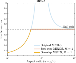
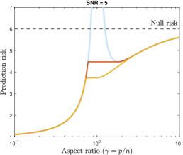
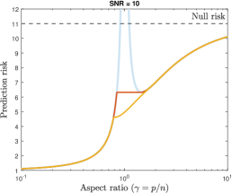
Figure 5: Comparison of zero-step and one-step procedures with MN2LS base procedures under isotropic feature covariance, and low, moderate, and high SNR regimes. Observe that for SNR = 1, zero-step and one-step both have the same risk profile with $M=1$. This holds true even for SNR $\leq$ 1, as shown in Theorem S.6.16. For SNR $>1$, there exists a range of $\gamma$ for which one-step is strictly better than zero-step. See Theorem S.6.16 for more details.

4.4 Numerical illustrations

In this section, we provide numerical illustration of the risk monotonization of one-step prediction procedure in the proportional asymptotic regime, when the base prediction procedures are MN2LS and MN1LS prediction procedures, and the one-step adjustment is always performed via MN2LS. In order to illustrate risk monotonization as in Theorem 4.4, we need to show the risk behavior of ${\widehat{f}}^{\mathrm{os}}$ at different aspect ratios. We use the same simulation settings used for the illustration of the zero-step procedure in Section 3.4. Figures 6 and 7 present our simulation results. The conclusions are essentially the same as those stated for the zero-step procedure in Section 3.4.

Minimum $\ell_{2}$-norm least squares (MN2LS).

Figure 6 shows the risks of the baseline MN2LS procedure and the one-step prediction procedure with MN2LS as the base prediction procedure for high and low SNR regimes (left: SNR = 4; right: SNR = 1); we take $\sigma^{2}=1$, so that $\rho^{2}$=SNR. We also present the null risk ($\rho^{2}+\sigma^{2}$), i.e., the risk of the zero predictor as a baseline in both the plots.

Similar to the behavior of the zero-step procedure we observe that the risk of the one-step procedure is non-decreasing in $\gamma$ for every $M\geq 1$. Although the risk of the one-step procedure is close to being below the risk of the base procedure, Figure 6 shows the effects of working with a finite sample. (The risk of one-step for $M=1$ is sometimes above the risk of the base procedure.)

Figure 6 also shows that the one-step prediction procedure can be strictly better than the zero-step prediction procedure. In particular, the left panel of Figure 6 shows that around the interpolation threshold of $1$, the risk of one-step prediction procedure is not flat. It is strictly increasing. The risk of one-step procedure for $M>1$ is once again seen to be a strict improvement over $M=1$.

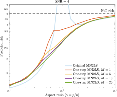
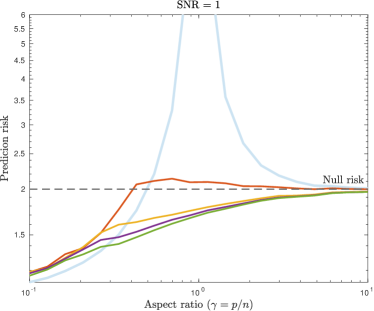
Figure 6: Illustration of the one-step procedure with the MN2LS as the base predictor and MN2LS one-step adjustment with varying $M$. The left panel shows a high SNR setting (SNR = 4), while the right panel shows a low SNR setting (SNR = 1). The setup has $n=1000$, $n_{\mathrm{tr}}=900$, $n_{\mathrm{te}}=100$, $n^{\nu}=50$. The features are drawn from an isotropic Gaussian distribution, the response follows a linear model with dense signal. The risks are averaged over 100 dataset repetitions.

Minimum $\ell_{1}$-norm least squares (MN1LS).

Figure 7 shows the risks of the baseline MN1LS procedure and the one-step procedure with MN1LS as the base prediction procedure for high (left, SNR = 4) and low (right, SNR = 1) SNR regimes. We take $\sigma^{2}=1$ and $\rho^{2}=$ SNR. We also present the null risk ($\rho^{2}+\sigma^{2}$), i.e., the risk of the zero predictor as a baseline in both the plots. We again observe that the risk of the one-step procedure for every $M\geq 1$ is non-decreasing in $\gamma$. As before, once again we observe in Figure 7 that the one-step procedure with $M=1$ attains precise risk monotonization while zero-step with $M>1$ improves significantly upon the $M=1$ case when $\gamma$ is near one. All these comments hold for both low and high SNR regimes.

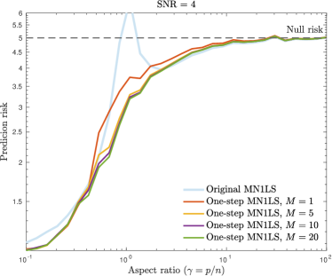
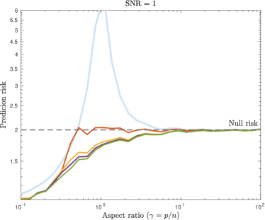
Figure 7: Illustration of the one-step procedure with MN1LS as the base procedure and MN2LS one-step adjustment with varying $M$. The left panel shows a high SNR setting (SNR = 4), while the right panel shows a low SNR setting (SNR = 1). In the setup, $n=500$, $n_{\mathrm{tr}}=420$, $n_{\mathrm{te}}=80$, $n^{\nu}=42$. The features are drawn from an isotropic Gaussian distribution, the response follows a linear model with sparse signal (sparsity level = 0.0005). The risks are averaged over 100 dataset repetitions.

5 Discussion

In this paper, we have proposed a generic cross-validation framework to monotonize any given prediction procedure in terms of the sample size. We studied two concrete methodologies: zero-step and one-step prediction procedures. The ingredient predictors for the zero-step prediction procedure is the base procedure applied on a subset of the data. The ingredient predictor for the one-step prediction procedure can be thought of as boosting applied to the base procedure learned on a subset of data (Schapire and Freund, (2013)). In both cases, we also introduced averaging over the subsets of the data (via the parameter $M$). This particular averaging step can be seen as bagging, which is known to have a variance reduction effect.

We have analyzed the properties of zero-step and one-step prediction procedures in a model-free setting under mild regularity assumptions. This is in contrast to many other works in this literature that require strong distributional assumptions. In part this is possible because we assume the existence of the limiting risk and monotonize it (in a data-driven way) without requiring the knowledge/form of the risk.

Monotonization of asymptotic risk also has implications for minimax risk. If the base prediction procedure has a finite asymptotic risk $\underline{R}$ and $\overline{R}$, respectively, at the limiting aspect ratios of $0$ and $\infty$, then both zero-step and one-step prediction procedures applied to such a base procedure yield predictors whose asymptotic risk lies between $[\underline{R},\overline{R}]$ for all limiting aspect ratios. For example, for the squared error loss and a linear model, the MN1LS and MN2LS predictors have $\underline{R}=\sigma^{2}$ and $\overline{R}=\|\beta_{0}\|_{\Sigma}^{2}+\sigma^{2}$, where $\sigma^{2}$ is the noise energy, which is also the unavoidable prediction risk, and $\|\beta_{0}\|_{\Sigma}^{2}$ is the effective signal energy. Because $\sigma^{2}$ is the unavoidable prediction risk, and hence a minimax lower bound, the zero-step and one-step predictors based on MN1LS and MN2LS are minimax optimal up to a multiplicative factor of $1~{}+~{}\text{SNR}=1~{}+~{}\|\beta_{0}\|_{\Sigma}^{2}/{\sigma^{2}}$ over all aspect ratios ranging from $0$ to $\infty$. Any base prediction procedure that leads to the null predictor (i.e., ${\widehat{f}}(x)=0$ for all $x$) for the limiting aspect ratio of $\infty$ also has the same property. (Most reasonable prediction procedures would yield the null predictor as the limiting aspect ratio tends to $\infty$.) Furthermore, for every procedure, there exists another procedure (such as the zero-step) whose risk is at least as good and is monotone. Thus, the minimax risk is a monotone function of the limiting aspect ratio. To our knowledge, the minimax risk in the proportional asymptotics regime under generic signal structure is not available in the literature.

Although the focus of the current paper is exclusively on choosing optimal sample size, one could apply the cross-validation framework proposed for selecting optimal predictors from any collection. In particular, one can use our methodology to find optimal penalty parameter for ridge regression or lasso. It can also be used to select the number of random features in random features regression or kernel features in kernel regression, or more generally, the number of parameters in a neural network. In the latter case, our procedures will yield model-wise monotonicity (Nakkiran et al.,, 2019).

There are several interesting future directions that one can pursue. We will discuss three specific directions below.

Theoretical characterization of the effect of bagging.

We have only characterized the risk of the zero-step and one-step with $M=1$ in terms of the limiting risk of the base procedure. In this sense, we did not fully analyze the effect of bagging ($M>1$) for both zero-step and one-step procedures. It is of interest to characterize the effect of bagging:

What is the limiting risk of the zero-step and one-step procedures when $M>1$?

From the theory of $U$-statistics, it is expected that the risk for $M>1$ is non-increasing in $M$. It is hard to however argue that the risk of zero/one-step predictors is monotone in the limiting aspect ratio when $M>1$. The main difficulty lies in proving that the ingredient predictors for the zero-step procedure have an asymptotic risk profile for $M\geq 1$. Once this is guaranteed, the theory developed in Section 3.3.1 will readily imply that the zero-step procedure with $M>1$ has an asymptotic monotonic risk profile. We now briefly mention the difficulty in proving the existence of the asymptotic risk profile for the ingredient predictor when $M>1$.

For concreteness, consider the ingredient predictor of the zero-step prediction procedure with $M>1$ that uses $k_{n}\leq n$ observations. This is given by

$${\widetilde{f}}_{M}(x)=\frac{1}{M}\sum_{j=1}^{M}{\widetilde{f}}(x;\mathcal{D}_{\mathrm{tr}}^{j})\quad\text{ with }\quad|\mathcal{D}_{\mathrm{tr}}^{j}|=k_{n}.$$

Note that we take subsets $\mathcal{D}_{\mathrm{tr}}^{j}$ as independent and identically distributed subsets of size $k_{n}$ from the data and hence for $M=\infty$, we get

$${\widetilde{f}}_{\infty}(x;\mathcal{D}_{\mathrm{tr}})=\frac{1}{\binom{n}{k_{n}}}\sum_{1\leq i_{1}<\ldots<i_{k_{n}}\leq n_{\mathrm{tr}}}{\widetilde{f}}(x;\{(X_{i_{j}},Y_{i_{j}}):1\leq j\leq k_{n}\}).$$ (62)

This is a $U$-statistics of order $k_{n}$ for every fixed $x$ in terms of the training data. If $R({\widetilde{f}}(\cdot;\mathcal{D}_{\mathrm{tr}}^{j}))\xrightarrow{\text{p}}R^{\mathrm{det}}(\phi)$ whenever $p/k_{n}\to\phi$, then from the theory developed in Section 3.3.1, it follows that $R({\widehat{f}}^{\mathrm{zs}}_{M})\xrightarrow{\text{p}}\min_{\zeta\geq\gamma}R^{\mathrm{det}}(\zeta)$ under (PA($\gamma$)). Hence, the main difficulty in characterizing the effect of bagging lies in proving the existence of limit of $R({\widetilde{f}})$. For the squared error loss, it can be proved that (see Section S.6.11)

$$R({\widetilde{f}}_{M})=R({\widetilde{f}}_{\infty}(\cdot;\mathcal{D}_{\mathrm{tr}}))+\frac{1}{M}\frac{1}{\binom{n}{k_{n}}}\sum_{i_{1},\dots,i_{k_{n}}}\int\left({\widetilde{f}}(x;\{(X_{i_{j}},Y_{i_{j}}):1\leq j\leq k_{n}\})-{\widetilde{f}}_{\infty}(x;\mathcal{D}_{\mathrm{tr}})\right)^{2}\,\mathrm{d}P_{X_{0}}(x).$$ (63)

It is interesting to note that the risk of ${\widetilde{f}}_{M}$ only depends on $M$ as a linear function of $1/M$. If the base predictor ${\widetilde{f}}$ is non-zero almost surely, then the risk of ${\widetilde{f}}_{M}$ is a strictly decreasing function of $M$. Observe that (53) holds true even for $M=1$ and from our results, we know that the right hand side with $M=1$ has a finite deterministic approximation. This implies that each of the components in (53) is asymptotically bounded. Hence, as $M\to\infty$, we can conclude that $R({\widetilde{f}}_{M})-R({\widetilde{f}}_{\infty})\xrightarrow{\text{p}}0$.

Because $k_{n}\to\infty$ and $p/k_{n}\to\phi$, the second term in (63) above could be analyzed using deterministic representation for ${\widetilde{f}}(X_{0};\{(X_{i_{j}},Y_{i_{j}}):1\leq j\leq k_{n}\})$ (e.g., Theorem 1 of Liu and Dobriban, (2019) for ridge regression) and the theory of $U$-statistics. On the other hand, $R({\widetilde{f}}_{\infty})$ could also be similarly analyzed using deterministic representations and the theory of $U$-statistics. We leave this for future work.

Other variants of boosting.

In our empirical studies, we found that the one-step predictor (for $M=1$) which is a boosted version of the subsampled predictor has a much better performance than the zero-step predictor (with $M=1$), especially around the interpolation threshold. For reasons unclear to us currently, the performance of one-step predictor (for $M=1$) can be matched, at least in shape, by a zero-step predictor with some $M>1$. In this sense, the effect of one iterate boosting can be matched by the effect of multi-subsample bagging. Furthermore, as $M$ increases, both zero-step and one-step seem to approach the same limit in our empirical studies. The interesting aspect is that the work done by $M$ subsample bagging is achieved by one boosting iterate. This begs the question: is there a better boosting mechanism that can match zero-step predictors performance at $M=\infty$. In particular:

What are the other choices of one-step residual adjustments? And what is the “best” choice?

We have only analyzed the one-step residual adjustment done via MN2LS. Other choices are certainly possible: for instance, one could do MN1LS or minimum $\ell_{p}$-norm least squares or minimum $\ell_{2}$ robust least squares in the context of linear regression. It seems cumbersome to analyze each one of these residuals adjustments case-by-case and find the best choice. For general models, one can think of the residuals adjustment we proposed as a variant of Newton’s step for the squared error loss under homoscedasticity as mentioned in (41). The discussion of the “best” choice of the residual adjustment very much hinges on the question of what is the best predictor in a given model in the proportional asymptotics regime. Although we do not know the answer to this question, one can potentially target the question of deriving a residual adjustment that yields an asymptotic risk performance similar to that of the zero-step predictor with $M=\infty$. For any given predictor, is there a one iterate boosted version (i.e., one-step predictor with $M=1$) that achieves the same asymptotic performance as the $M$-subsample bagging with $M=\infty$?

Similar to the one-step predictor one can develop a $k$-step predictor by splitting the data into potentially $(k+1)$ batches and optimizing over the number of observations in each batch. This is analogues to $k$-iterate boosting as our one-step procedure (with $M=1$) is analogues to the one iterate boosting. This gets computationally intensive very quickly as $k$ increases. Furthermore, we believe that $k$-step predictor combined with bagging would yield the same asymptotic risk profile as the zero- and one-step predictors with $M=\infty$. In this sense, it seems a worth problem to investigate a better one iterate booster than to investigate the $k$-step predictor precisely.

Comparison with other regularization strategies.

On the surface, zero-step and one-step procedures might seem to use only a subset of the data, and hence might appear sub-optimal. Along the same lines, one might also wonder why not employ regularization techniques and optimize over the regularization parameter. To the first point, note that we make use of the whole data in estimating the risk and comparing predictors at different sample sizes, and hence make use of the full data. To the second point, it is somewhat surprising to report that optimally-regularized procedures such as ridge regression with optimal choice of penalty need not have monotone risk (in the limiting aspect ratio); see, for example, Figure 1 of Hastie et al., (2019). But our procedure will always lead to a monotone risk and hence makes better use of the data compared to optimum regularization procedures in general. Irrespective, it is still interesting to consider the relation between zero-step and one-step, and the optimum regularization procedures in cases where the latter has a monotone risk. In our empirical studies we found that in a well-specified linear model, zero-step and one-step procedures (with the MN2LS base procedure) with a large enough $M$ have asymptotic risk very close to the risk of the optimum ridge regression procedure. See the left panel of Figure 8. In a sparse linear regression model, zero-step and one-step procedures (with the MN1LS base procedure) with a large enough $M$ has asymptotic risk very close to the risk of the optimum lasso regression. It is also interesting to observe that the risk is monotone for optimally tuned lasso. See the right panel of Figure 8. The effect of both bagging and boosting with large $M$ in this case appears to be similar. In other words, thinking of the base procedures MN2LS and MN1LS as ridge and lasso, respectively, with zero penalty parameter, the zero- and one-step predictors with $M$ large attaining the same asymptotic risk as optimum ridge or lasso can be considered as finding optimal regularization for these procedures. Without explicitly formalizing the regularization predictor, zero- and one-step perform “optimal” implicit regularization. To what extent such similarity extends to other settings is an interesting future direction:

Under what conditions, do zero- and one-step predictors with MN2LS/MN1LS base predictor match the asymptotic risk profile of optimized regularization of ridge/lasso regression? What other base predictors (and corresponding classes of regularized predictors) does this phenomenon extend to?

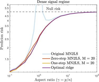
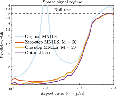
Figure 8: Comparison of different regularization strategies of zero-step, one-step, optimal ridge, and optimal lasso. The left panel shows a dense signal regime and the right panel shows a sparse signal regime. The setup has $n=100$, SNR = 4. The features are drawn from an isotropic Gaussian distribution, the response follows a linear model with dense (left panel) and sparse signal (right panel, sparsity level = $0.0005$). The risks are averaged over 100 dataset repetitions.

Supplement to “Mitigating multiple descents:
A model-agnostic framework for risk monotonization”

This document serves as a supplement to the paper “Mitigating multiple descents: A model-agnostic framework for risk monotonization.” The section and equation numbers in this document begin with the letters “S” and “E” to differentiate them from those in the main paper. The content of the document is organized as follows.

• In Section S.1, we present proofs of results related to general cross-validation and model selection from Sections 2.1 to 2.3.

• In Section S.2, we present proofs of results related to risk monotonization behavior of the zero-step procedure from Section 3.3.

• In Section S.3, we present proofs for the verification of the deterministic risk profile assumption for the MN2LS and MN1LS prediction procedures from Section 3.3.2.

• In Section S.4, we present proofs of results related to risk monotonization behavior of the one-step procedure from Section 4.3.1.

• In Section S.5, we present proofs for the verification of the deterministic risk profile assumption for arbitrary linear prediction procedures, and the MN2LS and MN1LS prediction procedures from Section 4.3.2.

• In Section S.6, we collect various technical helper lemmas and their proofs that are used in proofs in Sections S.2, S.3, S.4 and S.5, and other miscellaneous details.

• In Section S.7, we list calculus rules for a certain notion of asymptotic equivalence of sequences of matrices that are used in proofs in Sections S.3 and S.5.

• In Section S.8, we record statements of useful concentration results available in the literature that are used in proofs in Sections S.1, S.3 and S.5.

• In Section S.9, we list some of the main notation used in the paper.

S.1 Proofs related to general cross-validation and model selection

S.1.1 Proof of Proposition 2.1

Additive form.

We will first prove the oracle risk inequalities (7) in additive form. Recall Algorithm 1 returns ${\widehat{f}}^{\mathrm{cv}}={\widehat{f}}^{\widehat{\xi}}$. Adding and subtracting $\min_{\xi\in\Xi}R({\widehat{f}}^{\xi})$ and $\min_{\xi\in\Xi}{\widehat{R}}({\widehat{f}}^{\xi})$ to $R({\widehat{f}}^{\mathrm{cv}})$, we can break $R({\widehat{f}}^{\mathrm{cv}})$ into the following additive form:

$$R({\widehat{f}}^{\mathrm{cv}}) =\min_{\xi\in\Xi}R({\widehat{f}}^{\xi})+\min_{\xi\in\Xi}{\widehat{R}}({\widehat{f}}^{\xi})-\min_{\xi\in\Xi}R({\widehat{f}}^{\xi})-\min_{\xi\in\Xi}{\widehat{R}}({\widehat{f}}^{\xi})+R({\widehat{f}}^{\widehat{\xi}}).$$ (E.1)

An application of triangle inequality then lets us upper bound $R({\widehat{f}}^{\mathrm{cv}})$ into sum of three terms:

$$R({\widehat{f}}^{\mathrm{cv}})\leq\min_{\xi\in\Xi}R({\widehat{f}}^{\xi})+\underbrace{\Big{|}\min_{\xi\in\Xi}{\widehat{R}}({\widehat{f}}^{\xi})-\min_{\xi\in\Xi}R({\widehat{f}}^{\xi})\Big{|}}_{(a)}+\underbrace{\Big{|}R({\widehat{f}}^{\widehat{\xi}})-\min_{\xi\in\Xi}{\widehat{R}}({\widehat{f}}^{\xi})\Big{|}}_{(b)}.$$ (E.2)

We will next upper bound both terms (a) and (b) by $\Delta_{n}^{\mathrm{add}}$ to finish the first inequality of (7).

By definition (6a) of $\Delta_{n}^{\mathrm{add}}$, for every $\xi\in\Xi$, we can write

$$R({\widehat{f}}^{\xi})\leq{\widehat{R}}({\widehat{f}}^{\xi})+\Delta_{n}^{\mathrm{add}}\quad\text{and}\quad{\widehat{R}}({\widehat{f}}^{\xi})\leq R({\widehat{f}}^{\xi})+\Delta_{n}^{\mathrm{add}}.$$ (E.3)

Taking minimum on both sides of the inequalities in (E.3) then yields

$$\min_{\xi\in\Xi}{\widehat{R}}({\widehat{f}}^{\xi})\leq\min_{\xi\in\Xi}R({\widehat{f}}^{\xi})+\Delta_{n}^{\mathrm{add}}\quad\text{and}\quad\min_{\xi\in\Xi}R({\widehat{f}}^{\xi})\leq\min_{\xi\in\Xi}{\widehat{R}}({\widehat{f}}^{\xi})+\Delta_{n}^{\mathrm{add}}.$$

Combining the two inequalities, we arrive at the desired bound for term (a):

$$\Big{|}\min_{\xi\in\Xi}{\widehat{R}}({\widehat{f}}^{\xi})-\min_{\xi\in\Xi}R({\widehat{f}}^{\xi})\Big{|}\leq\Delta_{n}^{\mathrm{add}}.$$ (E.4)

Since ${\widehat{\xi}}\in\mathop{\mathrm{arg\,min}}_{\xi\in\Xi}{\widehat{R}}({\widehat{f}}^{\xi})$, we can obtain the following upper bound for term (b):

$$\Big{|}R({\widehat{f}}^{\widehat{\xi}})-\min_{\xi\in\Xi}{\widehat{R}}({\widehat{f}}^{\xi})\Big{|}=\left|R({\widehat{f}}^{\widehat{\xi}})-{\widehat{R}}({\widehat{f}}^{\widehat{\xi}})\right|\leq\Delta_{n}^{\mathrm{add}},$$ (E.5)

where the inequality follows from the definition of $\Delta_{n}^{\mathrm{add}}$.

Substituting the bounds (E.4) and (E.5) into (E.2), we conclude that

$$\Big{|}R({\widehat{f}}^{\mathrm{cv}})-\min_{\xi\in\Xi}R(\widehat{f}^{\xi})\Big{|}\leq 2\Delta_{n}^{\mathrm{add}}.$$ (E.6)

This implies the first inequality of (7). Taking expectations on the both sides of the first inequality of (7), we obtain

$$\mathbb{E}\big{[}R({\widehat{f}}^{\mathrm{cv}})\big{]}\leq\mathbb{E}\big{[}\min_{\xi\in\Xi}R(\widehat{f}^{\xi})\big{]}+2\mathbb{E}\big{[}\Delta_{n}^{\mathrm{add}}\big{]}.$$ (E.7)

It is clear that the first term on the right hand side is bounded above by $\min_{\xi\in\Xi}\mathbb{E}[R(\widehat{f}^{\xi})]$, and thus we obtain the second inequality of (7). This completes the proof of the oracle risk inequalities in additive form.

Multiplicative form.

We now turn to prove the oracle risk inequality (8) in multiplicative form. Recall again that Algorithm 1 returns ${\widehat{f}}^{\mathrm{cv}}={\widehat{f}}^{\widehat{\xi}}$. In contrast to the proof of Proposition 2.1, we now break $R({\widehat{f}}^{\mathrm{cv}})$ into the following multiplicative form:

$$R({\widehat{f}}^{\mathrm{cv}})=\frac{R({\widehat{f}}^{\mathrm{cv}})}{\widehat{R}({\widehat{f}}^{\mathrm{cv}})}\cdot\widehat{R}({\widehat{f}}^{\mathrm{cv}})~{} =~{}\frac{R({\widehat{f}}^{\mathrm{cv}})}{\widehat{R}({\widehat{f}}^{\mathrm{cv}})}\cdot\widehat{R}({\widehat{f}}^{\widehat{\xi}})$$

$$\overset{(i)}{=}\frac{R({\widehat{f}}^{\mathrm{cv}})}{{\widehat{R}}({\widehat{f}}^{\mathrm{cv}})}\cdot\min_{\xi\in\Xi}{\widehat{R}}({\widehat{f}}^{\xi})$$

$$=~{}\frac{R({\widehat{f}}^{\mathrm{cv}})}{{\widehat{R}}({\widehat{f}}^{\mathrm{cv}})}\cdot\min_{\xi\in\Xi}\left[\frac{{\widehat{R}}({\widehat{f}}^{\xi})}{R({\widehat{f}}^{\xi})}\cdot R({\widehat{f}}^{\xi})\right]$$

$$\overset{(ii)}{\leq}~{}\frac{R({\widehat{f}}^{\mathrm{cv}})}{{\widehat{R}}({\widehat{f}}^{\mathrm{cv}})}\cdot\min_{\xi\in\Xi}\left[\left(\max_{\rho\in\Xi}\frac{{\widehat{R}}({\widehat{f}}^{\rho})}{R({\widehat{f}}^{\rho})}\right)\cdot R({\widehat{f}}^{\xi})\right]$$

$${\leq}~{}\frac{R({\widehat{f}}^{\mathrm{cv}})}{{\widehat{R}}({\widehat{f}}^{\mathrm{cv}})}\cdot\left(\max_{\xi\in\Xi}\frac{{\widehat{R}}({\widehat{f}}^{\xi})}{R({\widehat{f}}^{\xi})}\right)\cdot\min_{\xi\in\Xi}R({\widehat{f}}^{\xi})$$

$$\overset{(iii)}{\leq}~{}\frac{\displaystyle 1}{\displaystyle\min_{\xi\in\Xi}\frac{{\widehat{R}}({\widehat{f}}^{\xi})}{R({\widehat{f}}^{\xi})}}\cdot\left(\max_{\xi\in\Xi}\frac{{\widehat{R}}({\widehat{f}}^{\xi})}{R({\widehat{f}}^{\xi})}\right)\cdot\min_{\xi\in\Xi}R({\widehat{f}}^{\xi})$$

$$=~{}\frac{\displaystyle\max_{\xi\in\Xi}\frac{{\widehat{R}}({\widehat{f}}^{\xi})}{R({\widehat{f}}^{\xi})}}{\displaystyle\min_{\xi\in\Xi}\frac{{\widehat{R}}({\widehat{f}}^{\xi})}{R({\widehat{f}}^{\xi})}}\cdot\min_{\xi\in\Xi}R({\widehat{f}}^{\xi}).$$ (E.8)

In the chain above, equality $(i)$ follows from the definition of ${\widehat{\xi}}$ in Algorithm 1, inequality $(ii)$ follows from the inequality $a_{i}b_{i}\leq(\max_{j}a_{j})b_{i}$ for any two sequences $a_{i},b_{i},1\leq i\leq m$, and inequality $(iii)$ follows by noting that

$$\frac{R({\widehat{f}}^{\mathrm{cv}})}{{\widehat{R}}({\widehat{f}}^{\mathrm{cv}})}=\frac{\displaystyle 1}{\displaystyle\frac{{\widehat{R}}({\widehat{f}}^{\mathrm{cv}})}{R({\widehat{f}}^{\mathrm{cv}})}}=\frac{\displaystyle 1}{\displaystyle\frac{{\widehat{R}}({\widehat{f}}^{\widehat{\xi}})}{R({\widehat{f}}^{\widehat{\xi}})}}\leq\frac{\displaystyle 1}{\displaystyle\min_{\xi\in\Xi}\frac{{\widehat{R}}({\widehat{f}}^{\xi})}{R({\widehat{f}}^{\xi})}}.$$

Now, from the definition of $\Delta_{n}^{\mathrm{mul}}$, for all $\xi\in\Xi$, we have

$$1-\Delta_{n}^{\mathrm{mul}}\leq\frac{{\widehat{R}}({\widehat{f}}^{\xi})}{R({\widehat{f}}^{\xi})}\leq 1+\Delta_{n}^{\mathrm{mul}}.$$

In addition, since the loss function is assumed to be non-negative, both $R({\widehat{f}}^{\xi})$ and ${\widehat{R}}({\widehat{f}}^{\xi})$ are non-negative for all $\xi$. Hence, we can bound

$$(1-\Delta_{n}^{\mathrm{mul}})_{+}\leq\min_{\xi\in\Xi}\frac{{\widehat{R}}({\widehat{f}}^{\xi})}{R({\widehat{f}}^{\xi})}\leq\max_{\xi\in\Xi}\frac{{\widehat{R}}({\widehat{f}}^{\xi})}{R({\widehat{f}}^{\xi})}\leq 1+\Delta_{n}^{\mathrm{mul}}.$$ (E.9)

Using (E.9) in (E.8) then implies the desired upper bound:

$$R(\widehat{f}^{\mathrm{cv}})\leq\frac{1+\Delta_{n}^{\mathrm{mul}}}{(1-\Delta_{n}^{\mathrm{mul}})_{+}}\cdot\min_{\xi\in\Xi}R({\widehat{f}}^{\xi}).$$

This completes the proof of the oracle risk inequality in multiplicative form.

S.1.2 Proof of Lemma 2.4

Tail bound.

We begin by applying the Bernstein inequality (see Lemma S.8.1 for the exact statement) on the random variables $\ell(Y_{j},{\widehat{f}}^{\xi}(X_{j})),j\in\mathcal{I}_{\mathrm{te}}$ with mean $R({\widehat{f}}^{\xi})$ conditionally on $\mathcal{D}_{\mathrm{tr}}$. (Note that the random variables are i.i.d. conditionally on $\mathcal{D}_{\mathrm{tr}}$.) For any $0<\eta<1$ and $\xi\in\Xi$, we have the tail bound

$$\mathbb{P}\left(\left|\frac{1}{|\mathcal{D}_{\mathrm{te}}|}\sum_{j\in\mathcal{I}_{\mathrm{te}}}\ell(Y_{j},{\widehat{f}}^{\xi}(X_{j}))-R({\widehat{f}}^{\xi})\right|\geq C_{1}\max\left\{\sqrt{\widehat{\sigma}_{\xi}^{2}\frac{\log\left(2/\eta\right)}{|\mathcal{D}_{\mathrm{te}}|}},\widehat{\sigma}_{\xi}\frac{\log\left(2/\eta\right)}{|\mathcal{D}_{\mathrm{te}}|}\right\}\,\mathrel{\Bigg{|}}\mathcal{D}_{\mathrm{tr}}\right)\leq\eta.$$ (E.10)

Taking expectation on both sides, we get that the unconditional probability is also bounded by $\eta$. Denoting the prediction risk estimate by ${\widehat{R}}({\widehat{f}}^{\xi})$, and choosing $\eta={\eta}/{|\Xi|}$, for any $\xi\in\Xi$, we can equivalently write the bound as

$$\mathbb{P}\left(\left|{\widehat{R}}({\widehat{f}}^{\xi})-R({\widehat{f}}^{\xi})\right|\geq C_{1}\widehat{\sigma}_{\xi}\max\left\{\sqrt{\frac{\log\left({2|\Xi|}/{\eta}\right)}{n_{\mathrm{te}}}},\frac{\log\left({2|\Xi|}/{\eta}\right)}{n_{\mathrm{te}}}\right\}\right)\leq\frac{\eta}{|\Xi|}.$$

Applying union bound over $\xi\in\Xi$, for any $0<\eta<1/|\Xi|$, we get uniform bound

$$\mathbb{P}\left(\max_{\xi\in\Xi}\left|{\widehat{R}}({\widehat{f}}^{\xi})-R({\widehat{f}}^{\xi})\right|\geq C_{1}\max_{\xi\in\Xi}\widehat{\sigma}_{\xi}\max\left\{\sqrt{\frac{\log\left({2|\Xi|}/{\eta}\right)}{n_{\mathrm{te}}}},\frac{\log\left({2|\Xi|}/{\eta}\right)}{n_{\mathrm{te}}}\right\}\right)\leq\eta.$$

Using the definition of $\Delta_{n}^{\mathrm{add}}$, and setting $\widehat{\sigma}_{\Xi}:=\max_{k\in\Xi}\widehat{\sigma}_{\xi}$, so far we have that

$$\mathbb{P}\left(\Delta_{n}^{\mathrm{add}}\geq C_{1}\widehat{\sigma}_{\Xi}\max\left\{\sqrt{\frac{\log\left({2|\Xi|}/{\eta}\right)}{n_{\mathrm{te}}}},\frac{\log\left({2|\Xi|}/{\eta}\right)}{n_{\mathrm{te}}}\right\}\right)\leq\eta.$$ (E.11)

Choosing $\eta=n^{-A}$ for $A>0$ provides the desired tail bound (for a modified constant $C_{1}>0$)

$$\mathbb{P}\left(\Delta_{n}^{\mathrm{add}}\geq C_{1}\widehat{\sigma}_{\Xi}\max\left\{\sqrt{\frac{\log\left(|\Xi|n^{A}\right)}{n_{\mathrm{te}}}},\frac{\log\left(|\Xi|n^{A}\right)}{n_{\mathrm{te}}}\right\}\right)\leq n^{-A}.$$

Expectation bound.

We now turn to bounding $\mathbb{E}[\Delta_{n}^{\mathrm{add}}]$. Define the event

$$\mathcal{B}_{n}^{\complement}:=\left\{\Delta_{n}^{\mathrm{add}}\geq C_{1}C_{2}\max\left\{\sqrt{\frac{\log\left(|\Xi|n^{A}\right)}{n_{\mathrm{te}}}},\frac{\log\left(|\Xi|n^{A}\right)}{n_{\mathrm{te}}}\right\}\right\}.$$

Since $\mathbb{P}(\widehat{\sigma}_{n}\geq C_{2})\leq n^{-A}$, combining this with (E.11), we conclude that $\mathbb{P}(\mathcal{B}_{n}^{\complement})\leq 2n^{-A}$. For the case of $\texttt{CEN}=\texttt{MOM}$, the proof follows from that of Lemma 2.5. This follows because bounded $\psi_{1}$ norm implies bounded $L_{2}$ norm.

We can bound $\mathbb{E}[\Delta_{n}^{\mathrm{add}}]$ by breaking the expected value as

$$\begin{split}\mathbb{E}[\Delta_{n}^{\mathrm{add}}]&=\mathbb{E}[\Delta_{n}^{\mathrm{add}}\mathbbm{1}_{\mathcal{B}_{n}}]+\mathbb{E}[\Delta_{n}^{\mathrm{add}}\mathbbm{1}_{\mathcal{B}_{n}^{\complement}}]\\ &\leq C_{1}C_{2}\max\left\{\sqrt{\frac{\log\left(|\Xi|n^{A}\right)}{n_{\mathrm{te}}}},\frac{\log\left(|\Xi|n^{A}\right)}{n_{\mathrm{te}}}\right\}+\left(\mathbb{E}[(\Delta_{n}^{\mathrm{add}})^{t}]\right)^{1/t}(\mathbb{P}(\mathcal{B}_{n}^{c}))^{1/r}\\ &\leq C_{1}C_{2}\max\left\{\sqrt{\frac{\log\left(|\Xi|n^{A}\right)}{n_{\mathrm{te}}}},\frac{\log\left(|\Xi|n^{A}\right)}{n_{\mathrm{te}}}\right\}+\left(\mathbb{E}[(\Delta_{n}^{\mathrm{add}})^{t}]\right)^{1/t}(2n^{-A})^{1/r},\end{split}$$ (E.12)

for Hölder conjugates $t,r\geq 2$ satisfying $1/t+1/r=1$. Observe now that

$$\mathbb{E}[(\Delta_{n}^{\mathrm{add}})^{t}] \leq|\Xi|\max_{\xi\in\Xi}\mathbb{E}\left[\big{|}\widehat{R}(\widehat{f}^{\xi})-R(\widehat{f}^{\xi})\big{|}^{t}\right]$$

$$\leq|\Xi|\max_{\xi\in\Xi}\mathbb{E}\left[\mathbb{E}\left[\big{|}\widehat{R}(\widehat{f}^{\xi})-R(\widehat{f}^{\xi})\big{|}^{t}\mathrel{\big{|}}\mathcal{D}_{\mathrm{tr}}\right]\right]$$

$$\leq C_{3}|\Xi|\max_{\xi\in\Xi}\mathbb{E}\left[\widehat{\sigma}_{\xi}^{t}\max\left\{\left(\frac{t}{n_{\mathrm{te}}}\right)^{t/2},\left(\frac{t}{n_{\mathrm{te}}}\right)^{t}\right\}\right],$$

where the last inequality follows from integrating the quantile bound in (E.10) and $C_{3}$ is a constant potentially larger than $C_{1}$. Substituting this bound in (E.12), we obtain the desired expectation bound

$$\begin{split}\mathbb{E}[\Delta_{n}^{\mathrm{add}}]&\leq C_{1}C_{2}\max\left\{\sqrt{\frac{\log\left(|\Xi|n^{A}\right)}{n_{\mathrm{te}}}},\frac{\log\left(|\Xi|n^{A}\right)}{n_{\mathrm{te}}}\right\}+C_{3}n^{-A/r}|\Xi|^{1/t}\max\left\{\sqrt{\frac{t}{n_{\mathrm{te}}}},\frac{t}{n_{\mathrm{te}}}\right\}\max_{\xi\in\Xi}\left(\mathbb{E}[\widehat{\sigma}_{\xi}^{t}]\right)^{1/t}.\end{split}$$

for $t,r\geq 2$ such that $1/r+1/t=1$. This completes the proof.

S.1.3 Proof of Lemma 2.5

Tail bound.

The proof is similar to the proof of Lemma 2.4. Our main workhorse is going to be Lemma S.8.2. We use $\eta=\big{(}|\Xi|n^{A}\big{)}^{-1}$ in Algorithm 1. Applying the lemma with such $\eta$ on the random variables $\ell(Y_{j},{\widehat{f}}^{\xi}(X_{j})),j\in\mathcal{I}_{\mathrm{te}}$ conditionally on $\mathcal{D}_{\mathrm{tr}}$, for each $\xi\in\Xi$ we get the tail bound

$$\mathbb{P}\left(\left|\frac{1}{|\mathcal{D}_{\mathrm{te}}|}\sum_{j\in\mathcal{I}_{\mathrm{te}}}\ell(Y_{j},{\widehat{f}}^{\xi}(X_{j}))-R({\widehat{f}}^{\xi})\right|\geq C_{1}\widehat{\sigma}_{\xi}\sqrt{\frac{\log(|\Xi|n^{A})}{|\mathcal{D}_{\mathrm{te}}|}}\,\mathrel{\Bigg{|}}\mathcal{D}_{\mathrm{tr}}\right)\leq\frac{n^{-A}}{|\Xi|}$$

for some absolute constant $C_{1}>0$. In other words,

$$\mathbb{P}\left(\left|{\widehat{R}}({\widehat{f}}^{\xi})-R({\widehat{f}}^{\xi})\right|\geq C_{1}\widehat{\sigma}_{\xi}\sqrt{\frac{\log(|\Xi|n^{A})}{n_{\mathrm{te}}}}\mathrel{\Bigg{|}}\mathcal{D}_{\mathrm{tr}}\right)\leq\frac{n^{-A}}{|\Xi|}.$$

Integrating out $\mathcal{D}_{\mathrm{tr}}$ and applying union bound over $\xi\in\Xi$ then leads to the uniform bound

$$\mathbb{P}\left(\max_{\xi\in\Xi}\left|{\widehat{R}}({\widehat{f}}^{\xi})-R({\widehat{f}}^{\xi})\right|\geq C_{1}\max_{\xi\in\Xi}\widehat{\sigma}_{\xi}\sqrt{\frac{\log(|\Xi|n^{A})}{n_{\mathrm{te}}}}\right)\leq n^{-A}.$$ (E.13)

Substituting for the definitions of $\Delta_{n}^{\mathrm{add}}$ and $\widehat{\sigma}_{\Xi}$ gives the desired tail bound

$$\mathbb{P}\left(\Delta_{n}^{\mathrm{add}}\geq C_{1}\widehat{\sigma}_{\Xi}\sqrt{\frac{\log(|\Xi|n^{A})}{n_{\mathrm{te}}}}\right)\leq n^{-A}.$$ (E.14)

Expectation bound.

For bounding $\mathbb{E}[\Delta_{n}^{\mathrm{add}}]$, we again follow similar strategy as in the proof of Lemma 2.4. In order to bound certain expectations, we begin by extending the tail bound (E.14). From the assumption, $\mathbb{P}(\widehat{\sigma}_{\Xi}\geq C_{2})\leq n^{-A}$ for a constant $C_{2}>0$. For such a constant, consider the event

$$\mathcal{B}_{n}^{\complement}:=\left\{\Delta_{n}^{\mathrm{add}}\geq C_{1}C_{2}\sqrt{\frac{\log(|\Xi|n^{A})}{n_{\mathrm{te}}}}\right\}.$$

Conditioning on the event $\{\widehat{\sigma}_{\Xi}\geq C_{2}\}$, we can bound the probability of $\mathcal{B}_{n}^{\complement}$ as follows:

$$\mathbb{P}(\mathcal{B}_{n}^{\complement}) =\mathbb{P}\left(\Delta_{n}^{\mathrm{add}}\geq C_{1}C_{2}\sqrt{\frac{\log(|\Xi|n^{A})}{n_{\mathrm{te}}}},\widehat{\sigma}_{\Xi}\leq C_{2}\right)+\mathbb{P}\left(\Delta_{n}^{\mathrm{add}}\geq C_{1}C_{2}\sqrt{\frac{\log(|\Xi|n^{A})}{n_{\mathrm{te}}}},\widehat{\sigma}_{\Xi}\geq C_{2}\right)$$

$$\leq\mathbb{P}\left(\Delta_{n}^{\mathrm{add}}\geq C_{1}\widehat{\sigma}_{\Xi}\sqrt{\frac{\log(|\Xi|n^{A})}{n_{\mathrm{te}}}}\right)+\mathbb{P}\left(\widehat{\sigma}_{n}\geq C_{2}\right)\leq\frac{2}{n^{A}},$$

where we used the bound from (E.14). We are now ready to bound $\mathbb{E}[\Delta_{n}^{\mathrm{add}}]$ by splitting using the event $\mathcal{B}_{n}^{\complement}$. We have

$$\mathbb{E}\left[\Delta_{n}^{\mathrm{add}}\right] =\mathbb{E}\left[\Delta_{n}^{\mathrm{add}}\mathbbm{1}_{\mathcal{B}_{n}}\right]+\mathbb{E}\left[\Delta_{n}^{\mathrm{add}}\mathbbm{1}_{\mathcal{B}_{n}^{\complement}}\right]$$

$$\leq C_{1}C_{2}\sqrt{\frac{\log(|\Xi|n^{A})}{n_{\mathrm{te}}}}+\left(\mathbb{P}(\mathcal{B}_{n}^{\complement})\right)^{1/2}\left(\mathbb{E}[|\Delta_{n}^{\mathrm{add}}|^{2}]\right)^{1/2}$$

$$\leq C_{1}C_{2}\sqrt{\frac{\log(|\Xi|n^{A})}{n_{\mathrm{te}}}}+\left(2n^{-A}\right)^{1/2}\left(\mathbb{E}[|\Delta_{n}^{\mathrm{add}}|^{2}]\right)^{1/2}$$ (E.15)

where in the first inequality, we used Cauchy-Schwartz inequality for the second term. It remains to bound $\mathbb{E}[|\Delta_{n}^{\mathrm{add}}|^{2}]$, which we do below. We have

$$\mathbb{E}[\left|\Delta_{n}^{\mathrm{add}}\right|^{2}] =\mathbb{E}\left[\max_{\xi\in\Xi}\left|{\widehat{R}}({\widehat{f}}^{\xi})-R({\widehat{f}}^{\xi})\right|^{2}\right]\leq|\Xi|\max_{\xi\in\Xi}\mathbb{E}\left[|{\widehat{R}}({\widehat{f}}^{\xi})-R({\widehat{f}}^{\xi})|^{2}\right].$$

For bounding the second term, recall that the MOM procedure computes ${\widehat{R}}({\widehat{f}}^{\xi})$ as the median of empirical means computed on $B$ partitions of the test data. For each of the $B$ partitions, the variance of the empirical mean is $\widehat{\sigma}_{\xi}^{2}/(n_{\mathrm{te}}/B)$. To bound the variance of the median of means on $B$ partitions, we invoke Theorem 1 of Gribkova, (2020) (with $k=2$, $\rho=1$, and $i$ corresponding to the median position). Note that each of the $B$ empirical means are independent and identically distributed. This provides

$$\mathbb{E}\left[\left|{\widehat{R}}({\widehat{f}}^{\xi})-R({\widehat{f}}^{\xi})\right|^{2}\mathrel{\Big{|}}\mathcal{D}_{\mathrm{tr}}\right] \leq C\left(\frac{\widehat{\sigma}_{\xi}^{2}}{n_{\mathrm{te}}/B}\right)\leq C\frac{B\widehat{\sigma}_{\xi}^{2}}{n_{\mathrm{te}}}.$$

for some absolute constant $C$. Thus,

$$\left(\mathbb{E}\left[|\Delta_{n}^{\mathrm{add}}|^{2}\right]\right)^{1/2} \leq C\left(|\Xi|\frac{B}{n_{\mathrm{te}}}\max_{\xi\in\Xi}\mathbb{E}[\widehat{\sigma}_{\xi}^{2}]\right)^{1/2}$$

$$\leq C|\Xi|^{1/2}\sqrt{\frac{B}{n_{\mathrm{te}}}}\max_{\xi\in\Xi}\Big{(}\mathbb{E}[\widehat{\sigma}_{\xi}^{2}]\Big{)}^{1/2}$$

Recalling $B=\lceil 8\log(|\Xi|n^{A})\rceil$ and combining this bound with (E.15), we finally have the desired expectation bound

$$\mathbb{E}\left[\Delta_{n}^{\mathrm{add}}\right]\leq C_{1}C_{2}\sqrt{\frac{\log(|\Xi|n^{A})}{n_{\mathrm{te}}}}+C_{3}n^{-A/2}|\Xi|^{1/2}\sqrt{\frac{\log(|\Xi|n^{A})}{n_{\mathrm{te}}}}\max_{\xi\in\Xi}\Big{(}\mathbb{E}[\widehat{\sigma}_{\xi}^{2}]\Big{)}^{1/2}.$$

for some absolute constant $C_{3}>0$. This completes the proof.

S.1.4 Proof of Lemma 2.9

As argued in the proof of Lemma 2.4, using Lemma S.8.1, for any $A>0$, we have the tail bound:

$$\mathbb{P}\left(\left|{\widehat{R}}({\widehat{f}}^{\xi})-R({\widehat{f}}^{\xi})\right|\geq C\widehat{\sigma}_{\xi}\max\left\{\sqrt{\frac{\log(|\Xi|n^{A})}{|\mathcal{D}_{\mathrm{te}}|}},\frac{\log(|\Xi|n^{A})}{|\mathcal{D}_{\mathrm{te}}|}\right\}\mathrel{\Bigg{|}}\mathcal{D}_{\mathrm{tr}}\right)\leq\frac{n^{-A}}{|\Xi|}$$

for some universal constant $C>0$. By diving $R({\widehat{f}}^{\xi})$ on the both side of error event, and denoting $\widehat{\sigma}_{\xi}/R({\widehat{f}}^{\xi})$ by $\widehat{\kappa}_{\xi}$, equivalently we have

$$\mathbb{P}\left(\left|\frac{{\widehat{R}}({\widehat{f}}^{\xi})}{R({\widehat{f}}^{\xi})}-1\right|\geq C\widehat{\kappa}_{\xi}\max\left\{\sqrt{\frac{\log(|\Xi|n^{A})}{|\mathcal{D}_{\mathrm{te}}|}},\frac{\log(|\Xi|n^{A})}{|\mathcal{D}_{\mathrm{te}}|}\right\}\mathrel{\Bigg{|}}\mathcal{D}_{\mathrm{tr}}\right)\leq\frac{n^{-A}}{|\Xi|}.$$

Integrating over randomness in $\mathcal{D}_{\mathrm{tr}}$, and applying union bound over $\xi\in\Xi$, we obtain

$$\mathbb{P}\left(\max_{\xi\in\Xi}\bigg{|}\frac{{\widehat{R}}({\widehat{f}}^{\xi})}{R({\widehat{f}}^{\xi})}-1\bigg{|}\geq C\max_{\xi\in\Xi}\widehat{\kappa}_{\xi}\max\left\{\sqrt{\frac{\log(|\Xi|n^{A})}{n_{\mathrm{te}}}},\frac{\log(|\Xi|n^{A})}{n_{\mathrm{te}}}\right\}\right)\leq n^{-A}.$$

In other words, in terms $\Delta_{n}^{\mathrm{mul}}$ and $\widehat{\kappa}_{\Xi}$, we have

$$\mathbb{P}\left(\Delta_{n}^{\mathrm{mul}}\geq C\widehat{\kappa}_{\Xi}\max\left\{\sqrt{\frac{\log(|\Xi|n^{A})}{n_{\mathrm{te}}}},\frac{\log(|\Xi|n^{A})}{n_{\mathrm{te}}}\right\}\right)\leq n^{-A},$$

as desired. This completes the proof.

S.1.5 Proof of Lemma 2.10

As argued in the proof of Lemma 2.5, using Lemma S.8.2, for any $A>0$, we have the following tail bound:

$$\mathbb{P}\left(\left|{\widehat{R}}({\widehat{f}}^{\xi})-R({\widehat{f}}^{\xi})\right|\geq C\widehat{\sigma}_{\xi}\sqrt{\frac{\log(|\Xi|n^{A})}{|\mathcal{D}_{\mathrm{te}}|}}\mathrel{\Bigg{|}}\mathcal{D}_{\mathrm{tr}}\right)\leq\frac{n^{-A}}{|\Xi|}$$

for some universal constant $C>0$. By diving $R({\widehat{f}}^{\xi})$ on the both side of error event, and denoting $\widehat{\sigma}_{\xi}/R({\widehat{f}}^{\xi})$ by $\widehat{\kappa}_{\xi}$, we obtain

$$\mathbb{P}\left(\left|\frac{{\widehat{R}}({\widehat{f}}^{\xi})}{R({\widehat{f}}^{\xi})}-1\right|\geq C\widehat{\kappa}_{\xi}\sqrt{\frac{\log(|\Xi|n^{A})}{|\mathcal{D}_{\mathrm{te}}|}}\mathrel{\Bigg{|}}\mathcal{D}_{\mathrm{tr}}\right)\leq\frac{n^{-A}}{|\Xi|}.$$

Integrating over randomness in $\mathcal{D}_{\mathrm{tr}}$, and applying union bound over $\xi\in\Xi$, this implies that

$$\mathbb{P}\left(\max_{\xi\in\Xi}\bigg{|}\frac{{\widehat{R}}({\widehat{f}}^{\xi})}{R({\widehat{f}}^{\xi})}-1\bigg{|}\geq C\max_{\xi\in\Xi}\widehat{\kappa}_{\xi}\sqrt{\frac{\log(|\Xi|n^{A})}{n_{\mathrm{te}}}}\right)\leq n^{-A}.$$

Writing in terms $\Delta_{n}^{\mathrm{mul}}$ and $\widehat{\kappa}_{\Xi}$, we arrive at the desired bound:

$$\mathbb{P}\left(\Delta_{n}^{\mathrm{mul}}\geq C\widehat{\kappa}_{\Xi}\sqrt{\frac{\log(|\Xi|n^{A})}{n_{\mathrm{te}}}}\right)\leq n^{-A}.$$

This finishes the proof.

S.1.6 Proof of Proposition 2.14

Part 1.

For the first part, observe that $|\ell(Y_{0},{\widehat{f}}(X_{0}))|=\max\{0,1-Y_{0}{\widehat{f}}(X_{0})\}\leq 2$ assuming $|Y_{0}|\leq 1$ and $|{\widehat{f}}(X_{0})|\leq 1$. For a bounded random variable $Z$, $\|Z\|_{\psi_{2}}\lesssim\|Z\|_{\infty}$ (see, e.g., Example 2.5.8 of Vershynin, (2018)). Thus, the random variable $\ell(Y_{0},{\widehat{f}}(X_{0}))$ is conditionally sub-Gaussian with sub-Gaussian norm $2$ (up to constants), and consequently sub-exponential with the same sub-exponential norm upper bound. The conditional $L_{2}$ norm bound follows similarly.

Part 2.

The second part follows in the same vein by noting that $\ell(Y_{0},{\widehat{f}}(X_{0}))=\mathbbm{1}_{Y_{0}\neq{\widehat{f}}(X_{0})}$ only takes values $0$ or $1$, and Bernoulli random variables are sub-Gaussian with sub-Gaussian norm $1$ (up to constants) and hence sub-exponential with the same sub-exponential norm upper bound. The bound on the conditional $L_{2}$ norm follows analogously.

S.1.7 Proof of Theorem 2.15

An outline for the proof is already provided in Section 2.3. The theorem follows by combining the additive form of the oracle inequality from Proposition 2.1, along with the probabilistic bounds on $\Delta^{\mathrm{add}}$ from Lemmas 2.5 and 2.4, and the bounds on conditional $\psi_{1}$ and $L_{2}$ norm bounds from Proposition 2.14.

S.1.8 Proof of Proposition 2.16

Part 1.

For the first part, we bound the $\psi_{1}$ norm of the squared error by the squared $\psi_{2}$ norm of the error to get

$$\|\ell(Y_{0},{\widehat{f}}(X_{0}))\|_{\psi_{1}\mid\mathcal{D}_{n}}=\|(Y_{0}-X_{0}^{\top}{\widehat{\beta}})^{2}\|_{\psi_{1}\mid\mathcal{D}_{n}}\leq\|Y_{0}-X_{0}^{\top}{\widehat{\beta}}\|_{\psi_{2}\mid\mathcal{D}_{n}}^{2},$$ (E.16)

where the inequality follows by Lemma 2.7.7 of Vershynin, (2018). Note that for any $\beta\in\mathbb{R}^{p}$, we have

$$(Y_{0}-X_{0}^{\top}{\widehat{\beta}})=(Y_{0}-X_{0}^{\top}\beta)+X_{0}^{\top}(\beta-{\widehat{\beta}}).$$ (E.17)

Because $\|Z_{1}+Z_{2}\|_{\psi_{2}}\leq\|Z_{1}\|_{\psi_{2}}+\|Z\|_{\psi_{2}}$ we can bound

$$\|Y_{0}-X_{0}^{\top}{\widehat{\beta}}\|_{\psi_{2}\mid\mathcal{D}_{n}}\leq\|Y_{0}-X_{0}^{\top}\beta\|_{\psi_{2}}+\|X_{0}^{\top}(\beta-{\widehat{\beta}})\|_{\psi_{2}\mid\mathcal{D}_{n}}.$$ (E.18)

Noting that $Y_{0}-X_{0}^{\top}\beta=(Y_{0},X_{0})^{\top}(1,-\beta)$ and $(\beta-{\widehat{\beta}})$ is a fixed vector conditioned on $\mathcal{D}_{n}$, by using $\psi_{2}-L_{2}$ equivalence on $(X_{0},Y_{0})$, we have

$$\|Y_{0}-X_{0}^{\top}\beta\|_{\psi_{2}}\leq\tau\|Y_{0}-X_{0}^{\top}\beta\|_{L_{2}}\quad\text{and}\quad\|X_{0}^{\top}(\beta-{\widehat{\beta}})\|_{\psi_{2}\mid\mathcal{D}_{n}}\leq\tau\|X_{0}^{\top}(\beta-{\widehat{\beta}})\|_{L_{2}\mid\mathcal{D}_{n}}=\tau\|{\widehat{\beta}}-\beta\|_{\Sigma},$$ (E.19)

where in the last inequality we used the fact that $\mathbb{E}[X_{0}]=0$ and $\mathbb{E}[X_{0}X_{0}^{\top}]=\Sigma$. Thus, combining (E.16), (E.18), and (E.19), for $\beta\in\mathbb{R}^{p}$, we have

$$\|\ell(Y_{0}-X_{0}^{\top}{\widehat{\beta}})\|_{\psi_{1}\mid\mathcal{D}_{n}}\leq(\|Y_{0}-X_{0}^{\top}\beta\|_{\psi_{2}}+\|{\widehat{\beta}}-\beta\|_{\Sigma})^{2}.$$

Taking infimum over $\beta$, we have that for squared loss

$$\|\ell(Y_{0},{\widehat{f}}(X_{0}))\|_{\psi_{1}\mid\mathcal{D}_{n}}\leq\tau^{2}\inf_{\beta\in\mathbb{R}^{p}}(\|Y_{0}-X_{0}^{\top}\beta\|_{\psi_{2}}+\|{\widehat{\beta}}-\beta\|_{\Sigma})^{2},$$

as desired. This completes the proof of the first inequality in (15). For the second inequality in (15), using the $\psi_{2}-L_{2}$ equivalence on the vector $(X_{0},Y_{0})$, observe that

$$\mathbb{E}[\ell(Y_{0},{\widehat{f}}(X_{0}))\mid\mathcal{D}_{n}]=\mathbb{E}[(Y_{0}-X_{0}^{\top}{\widehat{\beta}})^{2}\mid\mathcal{D}_{n}]=\|Y_{0}-X_{0}^{\top}\|_{L_{2}\mid\mathcal{D}_{n}}^{2}.$$ (E.20)

Hence, from (E.16) and (E.20), we have

$$\frac{\|\ell(Y_{0},{\widehat{f}}(X_{0}))\|_{\psi_{1}\mid\mathcal{D}_{n}}}{\mathbb{E}[\ell(Y_{0},{\widehat{f}}(X_{0}))\mid\mathcal{D}_{n}]}\leq\frac{\|Y_{0}-X_{0}^{\top}{\widehat{\beta}}\|^{2}_{\psi_{2}\mid\mathcal{D}_{n}}}{\|Y_{0}-X_{0}^{\top}{\widehat{\beta}}\|^{2}_{L_{2}\mid\mathcal{D}_{n}}}=\left(\frac{\|(Y_{0},X_{0})(1,-{\widehat{\beta}})\|_{\psi_{2}\mid\mathcal{D}_{n}}}{\|(Y_{0},X_{0})(1,-{\widehat{\beta}})\|_{L_{2}\mid\mathcal{D}_{n}}}\right)^{2}\leq\tau^{2},$$

as desired. This completes the proof of the first part.

Part 2.

We now turn to the second part to bound the conditional $L_{2}$ norm of the square loss. For the square loss, note that

$$\|\ell(Y_{0},{\widehat{f}}(X_{0}))\|_{L_{2}\mid\mathcal{D}_{n}}^{2}=\mathbb{E}[(Y_{0}-{\widehat{f}}(X_{0}))^{4}\mid\mathcal{D}_{n}].$$ (E.21)

Using the decomposition (E.17) and triangle inequality with respect to the $L_{4}$ norm, we have

$$\mathbb{E}[(Y_{0}-X_{0}^{\top}{\widehat{\beta}})^{4}\mid\mathcal{D}_{n}]^{1/4}\leq\mathbb{E}[(Y_{0}-X_{0}^{\top}\beta)^{4}\mid\mathcal{D}_{n}]^{1/4}+\mathbb{E}[X_{0}^{\top}(\beta-{\widehat{\beta}})^{4}\mid\mathcal{D}_{n}]^{1/4}$$ (E.22)

Using the $L_{4}-L_{2}$ equivalence for $(Y_{0},X_{0})$, we can bound

$$\|Y_{0}-X_{0}^{\top}\beta\|_{L_{4}}\leq\tau\|Y_{0}-X_{0}^{\top}\beta\|_{L_{2}}\quad\text{and}\quad\|X_{0}^{\top}(\beta-{\widehat{\beta}})\|_{L_{4}\mid\mathcal{D}_{n}}\leq\tau\|X_{0}^{\top}(\beta-{\widehat{\beta}})\|_{L_{2}\mid\mathcal{D}_{n}}.$$ (E.23)

Thus, combining (E.21), (E.22), and (E.23), we have for any $\beta\in\mathbb{R}^{p}$,

$$\|(Y_{0},{\widehat{f}}(X_{0}))\|_{L_{2}\mid\mathcal{D}_{n}}\leq(\tau\|Y_{0}-X_{0}^{\top}\beta\|_{L_{2}}+\tau\|{\widehat{\beta}}-\beta\|_{\Sigma})^{2}\leq\tau^{2}(\|Y_{0}-X_{0}^{\top}\beta\|_{L_{2}}+\|{\widehat{\beta}}-\beta\|_{\Sigma})^{2}.$$

This completes the proof of first inequality in (16). For the second inequality of (16), note that

$$\frac{\|\ell(Y_{0},{\widehat{f}}(X_{0}))\|_{L_{2}\mid\mathcal{D}_{n}}}{\mathbb{E}[\ell(Y_{0},{\widehat{f}}(X_{0}))\mid\mathcal{D}_{n}]}\leq\frac{\|Y_{0}-{\widehat{f}}(X_{0})\|_{L_{4}\mid\mathcal{D}_{n}}^{2}}{\|Y_{0}-{\widehat{f}}(X_{0})\|_{L_{2}\mid\mathcal{D}_{n}}^{2}}=\left(\frac{\|(Y_{0},X_{0})(1,-{\widehat{\beta}})\|_{L_{4}\mid\mathcal{D}_{n}}}{\|(Y_{0},X_{0})(1,-{\widehat{\beta}})\|_{L_{2}\mid\mathcal{D}_{n}}}\right)^{2}\leq\tau^{2}.$$

This concludes the proof of the second part.

S.1.9 Proof of Proposition 2.17

The proof is similar to that of Proposition 2.16.

Part 1.

From the decomposition (E.17) and the triangle inequality on $\psi_{1}$ norm, we have for any $\beta\in\mathbb{R}^{p}$,

$$\|Y_{0}-X_{0}^{\top}{\widehat{\beta}}\|_{\psi_{1}\mid\mathcal{D}_{n}}\leq\|Y_{0}-X_{0}^{\top}\beta\|_{\psi_{1}}+\|X_{0}^{\top}(\beta-{\widehat{\beta}})\|_{\psi_{1}\mid\mathcal{D}_{n}}.$$ (E.24)

Using the $\psi_{1}-L_{1}$ equivalence of $(X_{0},Y_{0})$, note that

$$\|Y_{0}-X_{0}^{\top}\beta\|_{\psi_{1}}\leq\tau\|Y_{0}-X_{0}^{\top}\beta\|_{L_{1}}\quad\text{and}\quad\|X_{0}^{\top}(\beta-{\widehat{\beta}})\|_{\psi_{1}\mid\mathcal{D}_{n}}\leq\tau\|X_{0}^{\top}(\beta-{\widehat{\beta}})\|_{\psi_{1}\mid\mathcal{D}_{n}}.$$ (E.25)

Thus, from (E.24) and (E.25), for any $\beta\in\mathbb{R}^{p}$, we have

$$\|Y_{0}-X_{0}^{\top}{\widehat{\beta}}\|_{\psi_{1}\mid\mathcal{D}_{n}}\leq\tau(\|Y_{0}-X_{0}^{\top}\beta\|_{L_{1}}+\|X_{0}^{\top}({\widehat{\beta}}-\beta)\|_{L_{1}\mid\mathcal{D}_{n}}).$$

Now taking infimum over $\beta\in\mathbb{R}^{p}$ yields the first inequality of (18). To show the second inequality, observe that

$$\frac{\|\ell(Y_{0},{\widehat{f}}(X_{0}))\|_{\psi_{1}\mid\mathcal{D}_{n}}}{\mathbb{E}[\ell(Y_{0},{\widehat{f}}(X_{0}))\mid\mathcal{D}_{n}]}\leq\frac{\|Y_{0}-X_{0}^{\top}{\widehat{\beta}}\|_{\psi_{1}\mid\mathcal{D}_{n}}}{\|Y_{0}-X_{0}^{\top}{\widehat{\beta}}\|_{L_{1}\mid\mathcal{D}_{n}}}\leq\tau,$$

as desired. This finishes the proof.

Part 2.

The second part follows analogously to the first part by using the $L_{2}-L_{1}$ equivalence on $(X_{0},Y_{0})$.

S.1.10 Proof of Proposition 2.18

We start by writing the loss as

$$\ell(Y_{0},{\widehat{f}}(X_{0})) =Y_{0}\log(1+e^{-X_{0}^{\top}{\widehat{\beta}}})+(1-Y_{0})\log(1+e^{X_{0}^{\top}{\widehat{\beta}}})$$

$$=\mathrm{KL}(Y_{0},\,(1+\exp(-X_{0}^{\top}{\widehat{\beta}}))^{-1}).$$

Observe that the loss is non-negative since $\log(1+e^{t})\geq 0$ for all $t$.

Upper bounds on $\psi_{1}$ and $L_{2}$ norms.

We will first obtain an upper on the loss and consequently on the $\psi_{1}$ and $L_{2}$ norms of the loss. Because $Y_{0}$ takes values $0$ or $1$, we have that

$$\ell(Y_{0},{\widehat{f}}(X_{0})) \leq\max\big{\{}\log(1+e^{-X_{0}^{\top}{\widehat{\beta}}}),\log(1+e^{X_{0}^{\top}{\widehat{\beta}}})\big{\}}$$

$$\leq\log(1+e^{|X_{0}^{\top}{\widehat{\beta}}|}),$$

where the second inequality follows since $t\mapsto e^{t}$ is monotonically increasing in $t$. Now using the following bound on $\log(1+e^{|t|})$:

$$\log(1+e^{|t|})\leq\begin{cases}\log 2&\text{ if }e^{|t|}\leq 1\\ \log(2e^{|t|})=\log 2+|t|&\text{ otherwise},\end{cases}$$

we can upper bound the loss by

$$\ell(Y_{0},{\widehat{f}}(X_{0}))\leq|X_{0}^{\top}{\widehat{\beta}}|+\log 2.$$

Hence, we can upper bound the $\psi_{1}$ and $L_{2}$ norm of the loss as follows:

$$\|\ell(Y_{0},\widehat{f}(X_{0}))\|_{\psi_{1}\mid\mathcal{D}_{n}} \leq\log(2)+\|X_{0}^{\top}{\widehat{\beta}}\|_{\psi_{1}\mid\mathcal{D}_{n}},$$ (E.26)

$$(\mathbb{E}[\ell^{2}(Y_{0},\widehat{f}(X_{0}))\mid\mathcal{D}_{n}])^{1/2} \leq\log(2)+(\mathbb{E}[|X_{0}^{\top}{\widehat{\beta}}|^{2}\mid\mathcal{D}_{n}])^{1/2}.$$ (E.27)

Lower bound on expectation.

Next we obtain a lower bound on $\mathbb{E}[\ell(Y_{0},{\widehat{f}}(X_{0}))\mid\mathcal{D}_{n}]$. Setting $p(x)=\mathbb{E}[Y_{0}|X_{0}=x]$, it is clear that

$$\mathbb{E}[\ell(Y_{0},{\widehat{f}}(X_{0}))\mid\mathcal{D}_{n},X_{0}]=p(X_{0})\log(1+\exp(-X_{0}^{\top}{\widehat{\beta}}))+(1-p(X_{0}))\log(1+\exp(X_{0}^{\top}{\widehat{\beta}})).$$

Because $0<p_{\min}\leq\min\{p(x),1-p(x)\}$ for all $x$, we have

$$\mathbb{E}[\ell(Y_{0},{\widehat{f}}(X_{0}))\mid\mathcal{D}_{n}] \geq p_{\min}\,\mathbb{E}[\max\{\log(1+\exp(-X_{0}^{\top}{\widehat{\beta}})),\,\log(1+\exp(X_{0}^{\top}{\widehat{\beta}}))\}\mid\mathcal{D}_{n}]$$

$$=p_{\min}\,\mathbb{E}[\log(1+\exp(|X_{0}^{\top}{\widehat{\beta}}|))\mid\mathcal{D}_{n}]$$

$$\geq\frac{p_{\min}}{2}\,\mathbb{E}[\log(2)+|X_{0}^{\top}{\widehat{\beta}}|\mid\mathcal{D}_{n}]=\frac{p_{\min}}{2}(\log(2)+\mathbb{E}|X^{\top}_{0}{\widehat{\beta}}|),$$ (E.28)

where the second equality follows since $t\mapsto e^{t}$ is monotonically increasing in $t\in\mathbb{R}$, and the last inequality follows from the fact that $1/2\leq\log(1+\exp(x))/(\log(2)+x)\leq 1$ for all $x\geq 0$.

Using (E.26) and (E.28), we have

$$\frac{\|\ell(Y_{0},{\widehat{f}}(X_{0}))\|_{\psi_{1}\mid\mathcal{D}_{n}}}{\mathbb{E}[\ell(Y_{0},{\widehat{f}}(X_{0}))\mid\mathcal{D}_{n}]}\leq\frac{\|X_{0}^{\top}{\widehat{\beta}}\|_{\psi_{1}\mid\mathcal{D}_{n}}+\log(2)}{p_{\min}(\mathbb{E}[|X_{0}^{\top}{\widehat{\beta}}|\mid\mathcal{D}_{n}]+\log(2))/2}\leq\frac{\tau\|X_{0}^{\top}{\widehat{\beta}}\|_{L_{1}\mid\mathcal{D}_{n}}+\log(2)}{p_{\min}(\tau\|X_{0}^{\top}{\widehat{\beta}}\|_{L_{1}\mid\mathcal{D}_{n}}+\log(2))/2}=2\tau p_{\min}^{-1}.$$

This proves the first part of Proposition 2.18. A similar bound holds for the second inequality of Proposition 2.18 using upper bound from (E.27) and lower bound (E.28). This completes the proof.

S.1.11 Proof of Theorem 2.22

An outline for the proof is provided in Section 2.3. The theorem follows by combining the multiplicative form of the oracle inequality from Proposition 2.1, along with probabilistic bounds on $\Delta^{\mathrm{mul}}$ from Lemmas 2.9 and 2.10, and the bounds on ratio of conditional $\psi_{1}$ and $L_{1}$ norms, and $L_{2}$ and $L_{1}$ norms from Proposition 2.16.

S.2 Proofs related to risk monotonization for zero-step procedure

S.2.1 Proof of Theorem 3.4

An outline for the proof is already provided in Section 3.3. For the sake of completeness, we briefly summarize the main steps below.

The deterministic additive and multiplicative oracle risk inequalities from Proposition 2.1, along with probabilistic bounds from Lemmas 2.4, 2.5, 2.9 and 2.10, provide the following bound on the risk of the zero-step predictor

$$R({\widehat{f}}^{\mathrm{zs}})=\begin{cases}\min_{\xi\in\Xi_{n}}R({\widehat{f}}^{\xi})+O_{p}(1)\sqrt{\log n/n_{\mathrm{te}}}&\text{ if }\widehat{\sigma}_{\Xi}=O_{p}(1),\\ \min_{\xi\in\Xi_{n}}R({\widehat{f}}^{\xi})\big{(}1+O_{p}(1)\sqrt{\log n/n_{\mathrm{te}}}\big{)}&\text{ if }\widehat{\kappa}_{\xi}=O_{p}(1).\end{cases}$$ (E.29)

Depending on the value of $M$, we now bound the term $\min_{\xi\in\Xi_{n}}R({\widehat{f}}^{\xi})$ under the assumptions (DET*) or (DET).

Case of $M=1$.

Under (DET*), we have from (33),

$$\min_{\xi\in\Xi_{n}}R({\widehat{f}}^{\xi})=\min_{\xi\in\Xi_{n}}R({\widetilde{f}}(\cdot;\mathcal{D}_{\mathrm{tr}}^{\xi,1}))=R^{\mathrm{det}}_{\nearrow}(n;{\widetilde{f}})(1+o_{p}(1)).$$ (E.30)

Combining (E.30) with (E.29) yields

$$\begin{split}R({\widehat{f}}^{\mathrm{zs}})&=\begin{cases}R^{\mathrm{det}}_{\nearrow}(n;{\widetilde{f}})(1+o_{p}(1))+O_{p}(1)\sqrt{\log n/n_{\mathrm{te}}}&\text{ if }\widehat{\sigma}_{\Xi}=O_{p}(1)\\ R^{\mathrm{det}}_{\nearrow}(n;{\widetilde{f}})(1+o_{p}(1))&\text{ if }\widehat{\kappa}_{\Xi}=O_{p}(1)\end{cases}\\ &=R^{\mathrm{det}}_{\nearrow}(n;{\widetilde{f}})\begin{cases}1+o_{p}(1)+\sqrt{\log n/n_{\mathrm{te}}}/R^{\mathrm{det}}_{\nearrow}(n;{\widetilde{f}})&\text{ if }\widehat{\sigma}_{\Xi}=O_{p}(1)\\ 1+o_{p}(1)&\text{ if }\widehat{\kappa}_{\Xi}=O_{p}(1).\end{cases}\end{split}$$ (E.31)

Thus, under (O1) or (O2), we have ${|R({\widehat{f}}^{\mathrm{zs}})-R^{\mathrm{det}}_{\nearrow}(n;{\widetilde{f}})|}/{R^{\mathrm{det}}_{\nearrow}(n;{\widetilde{f}})}=o_{p}(1)$ as desired.

Case of $M>1$.

Under (DET), we have from (32),

$$\begin{split}\min_{\xi\in\Xi_{n}}R({\widehat{f}}^{\xi})\leq R^{\mathrm{det}}_{\nearrow}(n;{\widetilde{f}})(1+o_{p}(1)).\end{split}$$ (E.32)

Now similar to the case of $M=1$, combining (E.32) with (E.29), and under (O1) or (O2), we have that ${(R({\widehat{f}}^{\mathrm{zs}})-R^{\mathrm{det}}_{\nearrow}(n;{\widetilde{f}}))_{+}}/{R^{\mathrm{det}}_{\nearrow}(n;{\widetilde{f}})}=o_{p}(1)$ as claimed. This finishes the proof.

S.2.2 Proof of Lemma 3.8

Our goal is to verify (DETPA-0), i.e., existence of a deterministic profile $R^{\mathrm{det}}(\cdot;{\widetilde{f}})$ such that for all non-stochastic sequences $\xi^{\star}_{n}\in\mathop{\mathrm{arg\,min}}_{\xi\in\Xi_{n}}R^{\mathrm{det}}(p_{n}/n_{\xi};{\widetilde{f}})$ and $1\leq j\leq M$,

$$\frac{R({\widetilde{f}}(\cdot;\mathcal{D}_{\mathrm{tr}}^{\xi_{n}^{\star},j}))-R^{\mathrm{det}}(p_{n}/n_{\xi_{n}^{\star}};{\widetilde{f}})}{R^{\mathrm{det}}(p_{n}/n_{\xi_{n}^{\star}};{\widetilde{f}})}\xrightarrow{\text{p}}0,$$

as $n\to\infty$ under (PA($\gamma$)). Recall here ${\widetilde{f}}(\cdot;\mathcal{D}_{\mathrm{tr}}^{\xi_{n}^{\star},j})$, $1\leq j\leq M$, is a predictor trained on the dataset $\mathcal{D}_{\mathrm{tr}}^{\xi_{n}^{\star},j}$ of sample size $n_{\xi_{n}^{\star}}=n_{\mathrm{tr}}-\xi_{n}^{\star}\lfloor n^{\nu}\rfloor$ and feature dimension $p_{n}$. We will make a series of reductions to verify (DETPA-0) from the assumptions of Lemma 3.8.

First, note that $R({\widetilde{f}}(\cdot;\mathcal{D}_{\mathrm{tr}}^{\xi_{n},j}))$ for $1\leq j\leq M$ are identically distributed. It thus suffices to pick $j=1$, which we will do below and drop the index for notational brevity. Second, since $R({\widetilde{f}}(\cdot;\mathcal{D}_{k_{m}}))>0$ for all $k_{m}$, it suffices to show that as $n\to\infty$ under (PA($\gamma$)),

$$R({\widetilde{f}}(\cdot;\mathcal{D}_{\mathrm{tr}}^{\xi_{n}^{\star}}))-R^{\mathrm{det}}(p_{n}/n_{\xi_{n}^{\star}};{\widetilde{f}})\xrightarrow{\text{p}}0,\quad\text{where}\quad\xi_{n}^{\star}\in\mathop{\mathrm{arg\,min}}_{\xi\in\Xi_{n}}R^{\mathrm{det}}(p_{n}/n_{\xi};{\widetilde{f}}).$$

More explicitly, that for all $\epsilon>0$, it suffices to verify that as $n\to\infty$ under (PA($\gamma$)),

$$\mathbb{P}\big{(}{|R({\widetilde{f}}(\cdot;\mathcal{D}_{\mathrm{tr}}^{\xi_{n}^{\star}}))-R^{\mathrm{det}}(p_{n}/n_{\xi_{n}^{\star}};{\widetilde{f}})|}\geq\epsilon\big{)}\to 0,\quad\text{where}\quad\xi_{n}^{\star}\in\mathop{\mathrm{arg\,min}}_{\xi\in\Xi_{n}}R^{\mathrm{det}}(p_{n}/n_{\xi};{\widetilde{f}}).$$

Now, we will do our final reduction. Fix $\epsilon>0$. Define a sequence $\{h_{n}(\epsilon)\}_{n\geq 1}$ as follows:

$$h_{n}(\epsilon):=\mathbb{P}\big{(}{|R({\widetilde{f}}(\cdot;\mathcal{D}_{\mathrm{tr}}^{\xi_{n}^{\star}}))-R^{\mathrm{det}}(p_{n}/n_{\xi_{n}^{\star}};{\widetilde{f}})|}\geq\epsilon\big{)}.$$

From the discussion in Section 3.3.1, we know that $p_{n}/n_{\xi_{n}^{\star}}$ may not necessarily converge as $n\to\infty$. But applying Lemma S.6.3 on the sequence $\{h_{n}(\epsilon)\}_{n\geq 1}$, in order to verify that $h_{n}(\epsilon)\to 0$ as $n\to\infty$, it suffices to show that for any index subsequence $\{n_{k}\}_{k\geq 1}$, there exists a further subsequence $\{n_{k_{l}}\}_{l\geq 1}$ such that $h_{n_{k_{l}}}(\epsilon)\to 0$ as $l\to 0$. Towards that goal, fix an arbitrary index subsequence $\{n_{k}\}_{k\geq 1}$. We will appeal to Lemma S.6.5 to construct the desired subsequence $\{n_{k_{l}}\}_{l\geq 1}$ along which we will argue that $h_{n_{k_{l}}}\to 0$ provided the assumptions of Lemma 3.8 are satisfied. In particular, from Lemma S.6.1, note that since $n_{\mathrm{tr}}/n\to 1$ as $n\to\infty$, we have $\Pi_{\Xi_{n}}(\zeta)\to\zeta$ for any $\zeta\in[\gamma,\infty]$ as $n\to\infty$. Now applying Lemma S.6.5 on $R^{\mathrm{det}}(\cdot;{\widetilde{f}})$ and the grid $\Xi_{n}$ guarantees that for any subsequence $\{p_{n_{k}}/n_{\xi_{n_{k}}^{\star}}\}_{k\geq 1}$, there exists a subsequence $\{p_{n_{k_{l}}}/n_{\xi_{n_{k_{l}}}^{\star}}\}_{l\geq 1}$ such that as $l\to\infty$,

$$\frac{p_{n}}{n_{\xi^{\star}_{n_{k_{l}}}}}\to\phi\in\mathop{\mathrm{arg\,min}}_{\zeta\in[\gamma,\infty]}R^{\mathrm{det}}(\zeta;{\widetilde{f}}).$$ (E.33)

We will now show that $h_{n_{k_{l}}}(\epsilon)\to 0$ as $l\to\infty$ if the profile convergence assumption (DETPAR-0) of Lemma 3.8 is satisfied, i.e., for a dataset $\mathcal{D}_{k_{m}}$ with $k_{m}$ observations and $p_{m}$ features, there exists $R^{\mathrm{det}}(\cdot;{\widetilde{f}})$ such that

$$R({\widetilde{f}}(\cdot;\mathcal{D}_{k_{m}}))\xrightarrow{\text{p}}R^{\mathrm{det}}(\phi;{\widetilde{f}})\quad\text{whenever}\quad\frac{p_{m}}{k_{m}}\to\phi\in\mathop{\mathrm{arg\,min}}_{\zeta\in[\gamma,\infty]}R^{\mathrm{det}}(\zeta;{\widetilde{f}}).$$ (E.34)

This follows easily because the profile convergence condition (E.34) implies that as $l\to\infty$,

$$\mathbb{P}\left(\left|R({\widetilde{f}}(\cdot;\mathcal{D}_{\mathop{\mathrm{tr}}}^{\xi^{\star}_{n_{k_{l}}}}))-R^{\mathrm{det}}(\phi;{\widetilde{f}})\right|\geq\epsilon\right)\to 0\quad\text{whenever}\quad\frac{p_{n}}{n_{\xi^{\star}_{n_{k_{l}}}}}\to\phi\in\mathop{\mathrm{arg\,min}}_{\zeta\in[\gamma,\infty]}R^{\mathrm{det}}(\zeta;{\widetilde{f}}).$$

But since $R^{\mathrm{det}}(\cdot;{\widetilde{f}})$ is continuous at $\phi$, and $p_{n}/n_{\xi^{\star}_{n_{k_{l}}}}\to\phi\in\mathop{\mathrm{arg\,min}}_{\zeta\in[\gamma,\infty]}R^{\mathrm{det}}(\zeta;{\widetilde{f}})$ as $l\to\infty$ from (E.33) this implies that, as $l\to\infty$,

$$\mathbb{P}\left(\left|R({\widetilde{f}}(\cdot;\mathcal{D}_{\mathop{\mathrm{tr}}}^{\xi^{\star}_{n_{k_{l}}}}))-R^{\mathrm{det}}(p_{n}/n_{\xi^{\star}_{n_{k_{l}}}};{\widetilde{f}})\right|\geq\epsilon\right)=h(n_{k_{l}})\to 0.$$

This concludes the proof.

S.2.3 Proof of Proposition 3.9

In order to verify lower semicontinuity of $h$, if suffices to show that for any $t\in\mathbb{R}_{\geq 0}$, the set $\{x:h(x)\leq t\}$ is closed. Because $\lim_{x\to b^{-}}h(x)=\infty$ and $h$ continuous on $[a,b)$, there exists $b_{-}(t)<b$ such that $h(x)>t$ for all $x>b_{-}(t)$. Similarly, there exists $b_{+}(t)>b$ such that $h(x)>t$ for all $x<b_{+}(t)$. Note that

$$\{x:h(x)\leq t\}=\{x:h|_{[a,b_{-}(t)]}(x)\leq t\}\cup\{x:h|_{[b_{+}(t),c]}(x)\leq t\}.$$

Because $h$ is continuous on $[a,b_{-}(t)]$ and $[b_{+}(t),c]$, it is also lower semicontinuous on these intervals, and hence the corresponding level sets are closed. Because the intersection of two closed sets is closed, the statement follows.

S.2.4 Proof of Proposition 3.10

The proof builds on similar idea as that in the proof of Lemma S.6.7 and employs a proof by contradiction. However, since the random functions in this case (which are conditional prediction risks) are not simply indexed by $n$ (but also by other properties of the data distributions), we will need to do a bit more work.

We wish to show that $R^{\mathrm{det}}(\cdot;{\widetilde{f}})$ is continuous on $\mathcal{I}\in(0,\infty)$. We will first show that $R^{\mathrm{det}}(\cdot;{\widetilde{f}})$ is $\mathbb{Q}$-continuous (see Definition S.6.8) on $\mathcal{I}$ and use Lemma S.6.9 to lift $\mathbb{Q}$-continuity to $\mathbb{R}$-continuity. Towards showing $\mathbb{Q}$-continuity, for the sake of contradiction, suppose $R^{\mathrm{det}}(\cdot;{\widetilde{f}})$ is $\mathbb{Q}$-discontinuous at some point $\phi_{\infty}\in\mathcal{I}$. This implies that there exists a sequence $\{\phi_{r}\}_{r\geq 1}$ in $\mathbb{Q}_{>0}$ such that $\phi_{r}\to\phi_{\infty}$, but for some $\epsilon>0$ and all $r\geq 1$,

$$R^{\mathrm{det}}(\phi_{r};{\widetilde{f}})\notin[R^{\mathrm{det}}(\phi_{\infty};{\widetilde{f}})-2\epsilon,R^{\mathrm{det}}(\phi_{\infty};{\widetilde{f}})+2\epsilon].$$ (E.35)

(Note that $R^{\mathrm{det}}(\phi_{r};{\widetilde{f}})\not\to R^{\mathrm{det}}(\phi_{\infty};{\widetilde{f}})$ as $\phi_{r}\to\phi_{\infty}$.) The proof strategy is now to construct a sequence of datasets $\{\mathcal{D}^{\prime}_{k_{m}}\}_{m\geq 1}$ whose aspects ratios $p_{m}/k_{m}$ converge to $\phi_{\infty}$, but the conditional prediction risks $R({\widetilde{f}}(\cdot;\mathcal{D}^{\prime}_{k_{m}}))$ of predictors ${\widetilde{f}}(\cdot;\mathcal{D}^{\prime}_{k_{m}})$ trained on these datasets do not converge to $R^{\mathrm{det}}(\phi_{\infty};{\widetilde{f}})$, thereby supplying a contradiction to the hypothesis of continuous convergence of $R({\widetilde{f}}(\cdot;\mathcal{D}^{\prime}_{k_{m}}))$ to $R^{\mathrm{det}}(\phi_{\infty};{\widetilde{f}})$. We will construct such a sequence of datasets below.

For every $r\geq 1$, construct a sequence of datasets $\{\mathcal{D}_{k_{m}}^{\phi_{r}}\}_{m\geq 1}$ with $k_{m}$ observations and $p_{m}=\phi_{i}k_{m}$ features. (Since $\phi_{r}\in\mathbb{Q}_{>0}$, the resulting $p_{m}$ is a positive integer.) See Figure S.1 for a visual illustration. For every $r\geq 1$, from the assumption of Proposition 3.10, we have that

$$R({\widetilde{f}}(\cdot;\mathcal{D}^{\phi_{r}}_{k_{m}}))\xrightarrow{\text{p}}R^{\mathrm{det}}(\phi_{r};{\widetilde{f}})$$ (E.36)

as $k_{m},p_{m}\to\infty$ because $p_{m}/k_{m}\to\phi_{r}$ as $m\to\infty$. Now, fix $p\in(0,1)$. For $r=1$, the convergence in (E.36) guarantees that there exists an integer $m_{1}\geq 1$ such that the event

$$\Omega_{m_{1}}:=\{|R({\widetilde{f}}(\cdot;\mathcal{D}^{\phi_{1}}_{k_{m_{1}}}))-R^{\mathrm{det}}(\phi_{1};{\widetilde{f}})|\leq\epsilon\}$$ (E.37)

has probability at least $p$. In addition, on the event $\Omega_{m_{1}}$, by the triangle inequality we have that

$$|R({\widetilde{f}}(\cdot;\mathcal{D}^{\phi_{1}}_{k_{m_{1}}}))-R^{\mathrm{det}}(\phi_{\infty};{\widetilde{f}})|\geq|R^{\mathrm{det}}(\phi_{1};{\widetilde{f}})-R^{\mathrm{det}}(\phi_{\infty};{\widetilde{f}})|-|R({\widetilde{f}}(\cdot;\mathcal{D}^{\phi_{1}}_{k_{m_{1}}}))-R^{\mathrm{det}}(\phi_{1};{\widetilde{f}})|>\epsilon,$$ (E.38)

where the second inequality follows by using (E.35) and (E.37). Next, for $r\geq 2$, let $m_{r}>m_{r-1}$ be an integer such that the event

$$\Omega_{m_{r}}:=\{|R({\widetilde{f}}(\cdot;\mathcal{D}^{\phi_{r}}_{k_{m_{r}}}))-R^{\mathrm{det}}(\phi_{r};{\widetilde{f}})|\leq\epsilon\}$$ (E.39)

has probability at least $p$. Such sequence of integers $\{m_{r}\}_{r\geq 2}$ and the associated events $\{\Omega_{m_{r}}\}_{r\geq 2}$ indeed exist as a consequence of the convergence in (E.36) for $r\geq 2$. On each $\Omega_{m_{r}}$

$$|R({\widetilde{f}}(\cdot;\mathcal{D}^{\phi_{r}}_{k_{m_{r}}}))-R^{\mathrm{det}}(\phi_{\infty};{\widetilde{f}})|>\epsilon$$

by similar reasoning as that for (E.38) using (E.35) and (E.39) for $r\geq 2$. Moreover, note that since $m_{r}>m$, $m_{r}\to\infty$ as $r\to\infty$.

Consider now a sequence of datasets $\{\mathcal{D}^{\prime}_{k_{m}}\}_{m\geq 1}$ such that:

1. The first $m_{1}$ datasets are $\{\mathcal{D}^{\phi_{1}}_{k_{m}}\}_{m=1}^{m_{1}}$ that have $k_{m}$ number of observations and $p_{m}=\phi_{1}k_{m}$ number of features for $m=1,\dots,m_{1}$.

2. The next $m_{2}-m_{1}$ datasets are $\{\mathcal{D}^{\phi_{2}}_{k_{m}}\}_{m=m_{1}+1}^{m_{2}}$ that have $k_{m}$ number of observations and $p_{m}=\phi_{2}k_{m}$ number of features for $m=m_{1}+1,\dots,m_{2}$.

3. The next $m_{3}-m_{2}$ datasets are $\{\mathcal{D}_{k_{m}}^{\phi_{3}}\}_{m=m_{2}+1}^{m_{3}}$ that have $k_{m}$ number of observations and $p_{m}=\phi_{3}k_{m}$ number of features for $m=m_{2}+1,\dots,m_{3}$.

4. And so on …

We will argue now that the sequence of datasets $\{\mathcal{D}^{\prime}_{k_{m}}\}_{m\geq 1}$ works for our promised contradiction. Observe that in the construction above the aspect ratios $p_{m}/k_{m}\to\phi_{\infty}$ because $\phi_{r}\to\phi_{\infty}$. However, we have that for all $r\geq 1$,

$$\mathbb{P}(|R({\widetilde{f}}(\cdot;\mathcal{D}^{\prime}_{k_{m_{r}}}))-R^{\mathrm{det}}(\phi_{\infty};{\widetilde{f}})|>\epsilon)=\mathbb{P}(|R({\widetilde{f}}(\cdot;\mathcal{D}_{k_{m_{r}}}))-R^{\mathrm{det}}(\phi_{\infty};{\widetilde{f}})|>\epsilon)\geq p.$$

Therefore, there exists an $\epsilon>0$ for which there is no $M\geq 1$ such that for $m\geq M$,

$$\mathbb{P}(|R({\widetilde{f}}(\cdot;\mathcal{D}^{\prime}_{k_{m}}))-R^{\mathrm{det}}(\phi_{\infty};{\widetilde{f}})|>\epsilon)<p/2.$$

Hence, we get the desired contraction that

$$R({\widetilde{f}}(\cdot;\mathcal{D}_{k_{m}}^{\prime}))\not\xrightarrow{\text{p}}R^{\mathrm{det}}(\phi_{\infty},{\widetilde{f}})$$

as $k_{m},p_{m}\to\infty$ and $p_{m}/k_{m}\to\phi_{\infty}$. This completes the proof.

It is worth pointing out that the proof above bears similarity to the proof of Lemma S.6.9. It is possible to combine the two and not have to go through the route of $\mathbb{Q}$-continuity. We, however, find it easier to break them so that the main ideas are easier to digest even though it leads to some repetition of overall proof strategies.

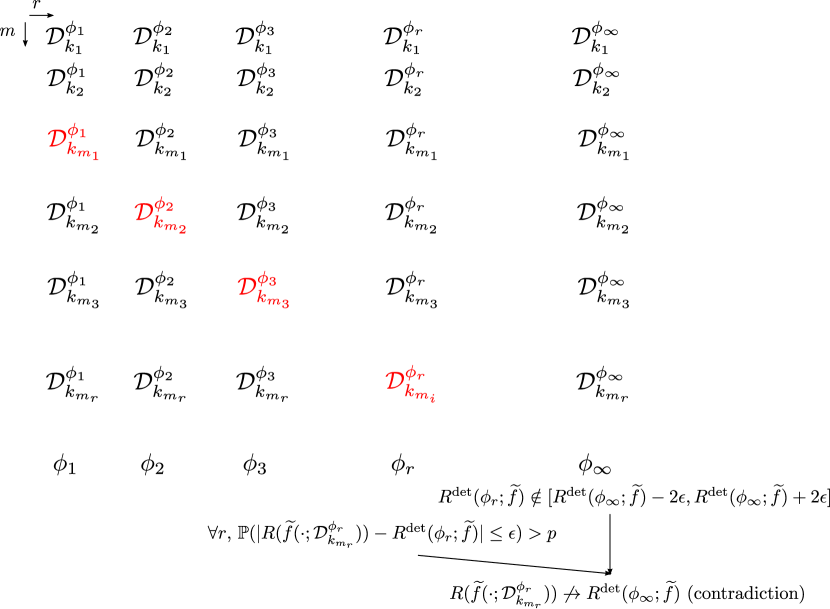
Figure S.1: Illustration of construction of grid of datasets used in the proof of Proposition 3.10. (Side note: as can be seen from the figure, the argument bears similarity to the standard diagonalization argument.)

S.2.5 Proof of Theorem 3.11

We will split the proof depending on the value of $M$.

Case of $M=1$.

Consider first the case when $M=1$. In this case, for every $\xi\in\Xi$, ${\widehat{f}}^{\xi}={\widetilde{f}}_{1}^{\xi}$ (and thus, ${\widetilde{f}}^{\star}={\widehat{f}}^{\mathrm{cv}}$), which we denote by ${\widetilde{f}}^{\xi}$ for simplicity of notation. To bound the desired difference, we break it into three terms:

$$\begin{split}\left(R({\widehat{f}}^{\mathrm{cv}})-\min_{\zeta\geq p/n}R^{\mathrm{det}}({\widetilde{f}};\zeta)\right)_{+}&=\left(R({\widehat{f}}^{\mathrm{cv}})-\min_{\xi\in\Xi}R({\widetilde{f}}^{\xi})\right)_{+}\\ &\quad+\left(\min_{\xi\in\Xi}R({\widetilde{f}}^{\xi})-\min_{\xi\in\Xi}R^{\mathrm{det}}\left({\widetilde{f}};\frac{p_{n}}{n_{\xi}}\right)\right)_{+}\\ &\quad+\left(\min_{\xi\in\Xi}R^{\mathrm{det}}\left({\widetilde{f}};\frac{p_{n}}{n_{\xi}}\right)-\min_{\zeta\geq p/n}R^{\mathrm{det}}({\widetilde{f}};\zeta)\right)_{+}.\end{split}$$ (E.40)

This inequality follows from the fact that $(a+b+c)_{+}\leq(a)_{+}+(b)_{+}+(c)_{+}$ for any $a,b,c\in\mathbb{R}$. We show below that each of the three terms asymptotically vanish in probability as $n\to\infty$ with $p/n\leq\Gamma$.

Term 1: Because $|\Xi|\leq n^{1-\nu}\leq n$, and $\widehat{\sigma}_{\Xi}=o_{p}(\sqrt{n^{\nu}/\log(n)})$, following Remark 2.8, under the assumptions of Lemma 2.4 or Lemma 2.5, we have

$$\left|R({\widetilde{f}}^{\mathrm{cv}})-\min_{\xi\in\Xi}R({\widetilde{f}}^{\xi})\right|=o_{p}(1),$$ (E.41)

which proves that the first term on the right hand side of (E.40) converges to zero in probability.

Term 2: To deal with the second term on the right hand side of (E.40), define

$$\xi_{n}^{\star}~{}\in~{}\mathop{\mathrm{arg\,min}}_{\xi\in\Xi}\,R^{\mathrm{det}}\left(\widetilde{f};\,\frac{p_{n}}{n_{\xi}}\right).$$

Because $R^{\mathrm{det}}(\cdot;\cdot)$ is a non-stochastic function, $\{\xi_{n}^{\star}\}_{n\geq 1}$ is a non-stochastic sequence and further, trivially, $\xi_{i}^{\star}\in\Xi$ for all $n\geq 1$. Observe now that

$$\begin{split}\min_{\xi\in\Xi}R(\widetilde{f}^{\xi})&\leq R(\widetilde{f}^{\xi_{n}^{\star}})\\ &=R(\widetilde{f}^{\xi_{n}^{\star}})-R^{\mathrm{det}}\left(\widetilde{f};\,\frac{p_{n}}{n_{\xi_{n}^{\star}}}\right)+\min_{\xi\in\Xi}\,R^{\mathrm{det}}\left(\widetilde{f};\,\frac{p_{n}}{n_{\xi}}\right).\end{split}$$ (E.42)

Hence, assumption (DETPA-0) implies that

$$\left(\min_{\xi\in\Xi}R(\widetilde{f}^{\xi})-\min_{\xi\in\Xi}\,R^{\mathrm{det}}\left(\widetilde{f};\,\frac{p_{n}}{n_{\xi}}\right)\right)_{+}=o_{p}(1),$$ (E.43)

as $n\to\infty$.

Term 3: Finally, because the risk profile $\zeta\mapsto R^{\mathrm{det}}({\widetilde{f}};\zeta)$ is assumed to be continuous at $\zeta^{\star}$, Lemma S.6.1 with the grid $\Xi$ yields

$$\left|\min_{\xi\in\Xi}R^{\mathrm{det}}\left({\widetilde{f}};\frac{p_{n}}{n_{\xi}}\right)-\inf_{\zeta\geq\gamma}R^{\mathrm{det}}({\widetilde{f}};\zeta)\right|=o(1).$$ (E.44)

Combining (E.41), (E.43), and (E.44), we have the desired result that

$$\left|R({\widehat{f}}^{\mathrm{cv}})-\min_{\zeta\geq\gamma}R^{\mathrm{det}}({\widetilde{f}};\zeta)\right|\xrightarrow{\text{p}}0.$$

Case of $M>1$.

Consider now the case when $M>1$. Note that $(x+y)_{+}\leq(x)_{+}+(y)_{+}$ since $\max\{z,0\}$ is a convex function of $z$. Thus, we can break and bound the desired difference as:

$$\left(R({\widehat{f}}^{\mathrm{cv}})-\min_{\zeta\geq p/n}R^{\mathrm{det}}({\widetilde{f}};\zeta)\right)_{+}$$

$$\leq\left(R({\widehat{f}}^{\mathrm{cv}})-\min_{\xi\in\Xi}R({\widehat{f}}^{\xi})\right)_{+}+\left(\min_{\xi\in\Xi}R({\widehat{f}}^{\xi})-\min_{\xi\in\Xi}\frac{1}{M}\sum_{j=1}^{M}R({\widetilde{f}}_{j}^{\xi})\right)_{+}$$

$$\quad+\left(\min_{\xi\in\Xi}\frac{1}{M}\sum_{j=1}^{M}R({\widetilde{f}}_{j}^{\xi})-\min_{\xi\in\Xi}R^{\mathrm{det}}\left({\widetilde{f}}^{\xi};\frac{p_{n}}{n_{\xi}}\right)\right)_{+}$$

$$\quad+\left(\min_{\xi\in\Xi}R^{\mathrm{det}}\left({\widetilde{f}};\frac{p_{n}}{n_{\xi}}\right)-\min_{\zeta\geq\gamma}R^{\mathrm{det}}({\widetilde{f}};\zeta)\right)_{+}.$$

As before, we show below that each of these terms are asymptotically vanishing in probability.

Term 1: Note that $\widehat{\sigma}_{\Xi}\leq{\widetilde{\sigma}}_{\Xi}$ (from the triangle inequality for $L_{2}$ and $\psi_{1}$ norms). Thus, as argued above for the case of $m=1$, the first term is $o_{p}(1)$.

Term 2: For the second term, observe that, for all $\xi\in\Xi$,

$$R\left({\widehat{f}}^{\xi}\right)=R\left(\frac{1}{M}\sum_{j=1}^{M}{\widetilde{f}}_{j}^{\xi}\right) =\mathbb{E}\left[\ell\left(Y_{0},\frac{1}{M}\sum_{i=1}^{M}{\widetilde{f}}_{j}^{\xi}(X_{0})\right)\mathrel{\Big{|}}\mathcal{D}_{1}\right]$$

$$\leq\frac{1}{M}\sum_{j=1}^{M}\mathbb{E}\left[\ell(Y_{0},{\widetilde{f}}_{j}^{\xi}(X_{0}))\mathrel{\big{|}}\mathcal{D}_{1}\right]$$

$$\leq\frac{1}{M}\sum_{j=1}^{M}R({\widetilde{f}}_{j}^{\xi}).$$

Therefore, we have

$$\min_{\xi\in\Xi}R({\widehat{f}}^{\xi})\leq\min_{\xi\in\Xi}\frac{1}{M}\sum_{j=1}^{M}R({\widetilde{f}}_{j}^{\xi})$$

and the second term is 0.

Term 3: For the third term, as before, note that

$$\left(\min_{\xi\in\Xi}\frac{1}{M}\sum_{j=1}^{M}R({\widetilde{f}}_{j}^{\xi})-\min_{\xi\in\Xi}R^{\mathrm{det}}\left({\widetilde{f}}^{\xi};\frac{p}{n_{\xi}}\right)\right)_{+}\leq\left(\frac{1}{M}\sum_{j=1}^{M}R({\widetilde{f}}_{j}^{\xi_{n}^{\star}})-R^{\mathrm{det}}\left({\widetilde{f}};\frac{p_{n}}{n_{\xi_{n}^{\star}}}\right)\right)_{+},$$

with the right hand side being $o_{p}(1)$ because of (DETPA-0).

Term 4: Analogous to the argument for the $m=1$ case, the fourth term is $o(1)$.

Combined together, we have the final result. This completes the proof. For an overview, a schematic for the proof of Theorem 3.11 is provided in Figure S.2.

Figure S.2: Schematic of the proof of Theorem 3.11.

S.3 Proofs related to deterministic profile verification for zero-step procedure

In this section, we verify the assumption (DETPAR-0) for the MN2LS and MN1LS prediction procedures.

S.3.1 Proof of Proposition 3.14

Recall $\mathcal{D}_{k_{m}}$ is a dataset with $k_{m}$ observations and $p_{m}$ features. Theorem 3 of Hastie et al., (2019) assumes the following distributional assumptions on the dataset $\mathcal{D}_{k_{m}}$.

1. The observations $(X_{i},Y_{i})$, $1\leq i\leq k_{m}$, are sampled i.i.d. from the model $Y_{i}=X_{i}^{\top}\beta_{0}+\varepsilon_{i}$ for some (deterministic) unknown signal vector $\beta_{0}\in\mathbb{R}^{p_{m}}$ and (random) unobserved error $\varepsilon_{i}$, assumed to be independent of $X_{i}\in\mathbb{R}^{p_{m}}$, with mean $0$, variance $\sigma^{2}$, and bounded moment of order $4+\delta$ for some $\delta>0$.

2. The feature vector $X_{i}$, $1\leq i\leq k_{m}$, decomposes as $X_{i}=\Sigma^{1/2}Z_{i}$, where $\Sigma\in\mathbb{R}^{p_{m}\times p_{m}}$ is a positive semidefinite (covariance) matrix and $Z_{i}\in\mathbb{R}^{p_{m}\times 1}$ is a random vector containing i.i.d. entries with mean $0$, variance $1$, and bounded moment of order $4+\delta$ for some $\delta>0$.

3. The norm of the signal vector $\|\beta_{0}\|_{2}$ is uniformly bounded in $p$, and $\lim_{p_{m}\to\infty}\|\beta_{0}\|_{2}^{2}=\rho^{2}<\infty$.

4. There exist real numbers $r_{\min}$ and $r_{\max}$ with $0<r_{\min}\leq r_{\max}<\infty$ such that $r_{\min}I_{p_{m}}~{}\preceq~{}\Sigma~{}\preceq~{}r_{\max}I_{p_{m}}$.

5. Let $\Sigma=WRW^{\top}$ denote the eigenvalue decomposition of the covariance matrix $\Sigma$, where $R\in\mathbb{R}^{p_{m}\times p_{m}}$ is a diagonal matrix containing eigenvalues (in non-increasing order) $r_{1}\geq r_{2}\geq\dots\geq r_{p_{m}}\geq 0$, and $W~{}\in~{}\mathbb{R}^{p_{m}\times p_{m}}$ is an orthonormal matrix containing the associated eigenvectors $w_{1},w_{2},\dots,w_{p_{m}}~{}\in~{}\mathbb{R}^{p_{m}}$. Let $H_{p_{m}}$ denote the empirical spectral distribution of $\Sigma$ (supposed on $\mathbb{R}_{>0}$) whose value at any $r\in\mathbb{R}$ is given by

   $$H_{p_{m}}(r)=\frac{1}{p_{m}}\sum_{i=1}^{p_{m}}\mathbbm{1}_{\{r_{i}\leq r\}}.$$

   Let $G_{p_{m}}$ denote a certain distribution (supported on $\mathbb{R}_{>0}$) that encodes the components of the signal vector $\beta_{0}$ in the eigenbasis of $\Sigma$ via the distribution of (squared) projection of $\beta_{0}$ along the eigenvectors $w_{j},1\leq j\leq p_{m}$, whose value any $r\in\mathbb{R}$ is given by

   $$G_{p_{m}}(r)=\frac{1}{\|\beta_{0}\|_{2}^{2}}\sum_{i=1}^{p_{m}}(\beta_{0}^{\top}w_{i})^{2}\,\mathbbm{1}_{\{r_{i}\leq r\}}.$$

   Assume there exist fixed distributions $H$ and $G$ (supported on $\mathbb{R}_{>0}$) such that $H_{p_{m}}\overset{d}{\to}H$ and $G_{p_{m}}\overset{d}{\to}G$ as $p_{m}\to\infty$.

Under assumptions ($\ell_{2}$A1)–($\ell_{2}$A5), we will verify that, for the MN2LS base prediction procedure ${\widetilde{f}}_{\mathrm{mn2}}$, there exists a deterministic risk approximation $R^{\mathrm{det}}(\cdot;{\widetilde{f}}_{\mathrm{mn2}}):(0,\infty]\to[0,\infty]$ that satisfy the two conditions stated in Proposition 3.14. In particular, we will show that the function $R^{\mathrm{det}}(\cdot;{\widetilde{f}}_{\mathrm{mn2}})$ defined below satisfies the required conditions:

$$R^{\mathrm{det}}(\phi;{\widetilde{f}}_{\mathrm{mn2}})=\begin{dcases}\sigma^{2}\frac{1}{1-\phi}&\text{ if }\phi\in(0,1)\\ \infty&\text{ if }\phi=1\\ \rho^{2}(1+\widetilde{v}_{g}(0;\phi))\int\frac{r}{(1+v(0;\phi)r)^{2}}\,\mathrm{d}G(r)\\ \quad+~{}\sigma^{2}\left(\phi\widetilde{v}(0;\phi)\int\frac{r^{2}}{(1+v(0;\phi)r)^{2}}\,\mathrm{d}H(r)+1\right)&\text{ if }\phi=(1,\infty)\\ \rho^{2}\int r\,\mathrm{d}G(r)+\sigma^{2}&\text{ if }\phi=\infty,\end{dcases}$$ (E.45)

where the scalars $v(0;\phi)$, $\widetilde{v}(0;\phi)$, and $\widetilde{v}_{g}(0;\phi)$, for $\phi\in(1,\infty)$, are defined as follows:

• $v(0;\phi)$ is the unique solution to the fixed-point equation:

  $$\frac{1}{\phi}=\int\frac{v(0;\phi)r}{1+v(0;\phi)r}\,\mathrm{d}H(r),$$ (E.46)

• $\widetilde{v}(0;\phi)$ is defined through $v(0;\phi)$ by the equation:

  $$\widetilde{v}(0;\phi)=\left(\frac{1}{v(0;\phi)^{2}}-\phi\int\frac{r^{2}}{(1+v(0;\phi)r)^{2}}\,\mathrm{d}H(r)\right)^{-1},$$ (E.47)

• $\widetilde{v}_{g}(0;\phi)$ is defined through $v(0;\phi)$ and $\widetilde{v}(0;\phi)$ by the equation:

  $$\widetilde{v}_{g}(0;\phi)=\widetilde{v}(0;\phi)\phi\int\frac{r^{2}}{(1+v(0;\phi)r)^{2}}\,\mathrm{d}H(r).$$ (E.48)

We will verify the two conditions of Proposition 3.14 below.

The limiting risk for the MN2LS predictor provided in (E.45), although in a different notation, matches the one obtained in Theorem 3 of Hastie et al., (2019). We believe our notation makes the subsequent analysis for the one-step procedure easy to follow for the reader. It is worth mentioning, however, that Hastie et al., (2019) only explicitly consider $\phi\in(0,1)\cup(1,\infty)$. We extend the analysis to show that the risk continuously diverges to $\infty$ as $\phi\to 1$ and also continuously converges to the null risk as $\phi\to\infty$. In addition, as mentioned in Remark 3.16, we analyze the prediction risk conditioned on both $(\bm{X},\bm{Y})$ as opposed to only on $\bm{X}$ as done in Hastie et al., (2019). Furthermore, we also establish continuity properties of the deterministic risk approximation in the aspect ratio that is needed for our analysis.

Condition 1: Continuous convergence of conditional risk over $\phi\in(0,1)\cup(1,\infty]$.

Let $\bm{X}\in\mathbb{R}^{k_{m}\times p_{m}}$ denote the design matrix and $\bm{Y}\in\mathbb{R}^{k_{m}}$ denote the response vector associated with the dataset $\mathcal{D}_{k_{m}}$. Let $\bm{\varepsilon}\in\mathbb{R}^{k_{m}}$ denote the error vector containing errors $\varepsilon_{i}$, $1\leq i\leq k_{m}$. Write the data model from assumption ($\ell_{2}$A1) as $\bm{Y}=\bm{X}^{\top}\beta_{0}+\bm{\varepsilon}$, and the MN2LS estimator (20) as

$${\widetilde{\beta}}_{\mathrm{mn2}}(\mathcal{D}_{k_{m}})=(\bm{X}^{\top}\bm{X}/k_{m})^{\dagger}\bm{X}^{\top}\bm{Y}/k_{m}.$$ (E.49)

The associated predictor ${\widetilde{f}}_{\mathrm{mn2}}(\cdot;\mathcal{D}_{k_{m}})$ is given by (22). Recall the prediction risk $R_{\bm{X},\bm{Y}}({\widetilde{f}}_{\mathrm{mn2}}(\cdot;\mathcal{D}_{k_{m}}))$ (where we use the subscripts $\bm{X},\bm{Y}$ to explicitly indicate the dependence of $R({\widetilde{f}}_{\mathrm{mn2}}(\cdot;\mathcal{D}_{k_{m}}))$ on the training data $(\bm{X},\bm{Y})$) under the squared error loss is given by

$$R_{\bm{X},\bm{Y}}({\widetilde{f}}_{\mathrm{mn2}}(\cdot;\mathcal{D}_{k_{m}}))=\mathbb{E}[(Y_{0}-{\widetilde{f}}_{\mathrm{mn2}}(X_{0};\mathcal{D}_{k_{m}}))^{2}\mid\bm{X},\bm{Y}],$$ (E.50)

where $(X_{0},Y_{0})$ is sampled independently from the same distribution as the training data $(\bm{X},\bm{Y})$.

Our goal is to show that as $k_{m},p_{m}\to\infty$, if $p_{m}/k_{m}\to\phi\in(0,1)\cup(1,\infty]$, $R_{\bm{X},\bm{Y}}({\widetilde{f}}_{\mathrm{mn2}}(\cdot;\mathcal{D}_{k_{m}}))\xrightarrow{\text{a.s.}}R^{\mathrm{det}}(\phi;{\widetilde{f}}_{\mathrm{mn2}})$. The proof follows by combining Propositions S.3.1, S.3.2 and S.3.3. Specifically:

1. Propositions S.3.1 and S.3.2 combined together imply that $R_{\bm{X},\bm{Y}}({\widetilde{f}}_{\mathrm{mn2}}(\cdot;\mathcal{D}_{k_{m}}))\xrightarrow{\text{a.s.}}R^{\mathrm{det}}(\phi;{\widetilde{f}}_{\mathrm{mn2}})$ as $p_{m},k_{m}\to\infty$ and $p_{m}/k_{m}\to\phi\in(0,1)\cup(1,\infty)$.

2. Proposition S.3.3 imply that $R_{\bm{X},\bm{Y}}({\widetilde{f}}_{\mathrm{mn2}}(\cdot;\mathcal{D}_{k_{m}}))\xrightarrow{\text{a.s.}}R^{\mathrm{det}}(\infty;{\widetilde{f}}_{\mathrm{mn2}})$ as $p_{m},k_{m}\to\infty$ and $p_{m}/k_{m}\to\infty$.

Below we prove Propositions S.3.1 to S.3.3.

In preparation for the statements to follow, denote by ${\widehat{\bm{\Sigma}}}:=\bm{X}^{\top}\bm{X}/k_{m}$ the sample covariance matrix. Let the singular value decomposition of $\bm{X}/\sqrt{k_{m}}$ be $\bm{X}/\sqrt{k_{m}}=\bm{U}\bm{S}\bm{V}^{\top}$, where $\bm{U}\in\mathbb{R}^{k_{m}\times k_{m}}$ and $\bm{V}\in\mathbb{R}^{p_{m}\times p_{m}}$ are orthonormal matrices, and $\bm{S}\in\mathbb{R}^{k_{m}\times p}$ is a diagonal matrix containing singular values in non-increasing order $s_{1}\geq s_{2}\geq\dots$.

The proposition below provides conditional convergence for the prediction risk (E.50) when $p_{m}/k_{m}\to\phi\in(0,1)\cup(1,\infty)$ as $p_{m},k_{m}\to\infty$.

Proposition S.3.1 (Conditional convergence of squared prediction risk of MN2LS predictor).

Suppose assumptions ($\ell_{2}$A1)–($\ell_{2}$A4) hold. Then, as $k_{m},p_{m}\to\infty$, if $p_{m}/k_{m}\to\phi\in(0,1)\cup(1,\infty)$, then

$$R_{\bm{X},\bm{Y}}({\widetilde{f}}_{\mathrm{mn2}}(\cdot;\mathcal{D}_{k_{m}}))-\beta_{0}^{\top}(I_{p_{m}}-{\widehat{\bm{\Sigma}}}^{\dagger}{\widehat{\bm{\Sigma}}})\Sigma(I_{p_{m}}-{\widehat{\bm{\Sigma}}}^{\dagger}{\widehat{\bm{\Sigma}}})\beta_{0}-\sigma^{2}\mathop{\mathrm{tr}}[{\widehat{\bm{\Sigma}}}^{\dagger}\Sigma]/k_{m}-\sigma^{2}\xrightarrow{\text{a.s.}}0.$$ (E.51)

Proof.

Under assumption ($\ell_{2}$A1), the squared prediction risk (E.50) decomposes into

$$R_{\bm{X},\bm{Y}}({\widetilde{f}}_{\mathrm{mn2}}(\cdot;\mathcal{D}_{k_{m}}))=({\widetilde{\beta}}_{\mathrm{mn2}}(\mathcal{D}_{k_{m}})-\beta_{0})^{\top}\Sigma({\widetilde{\beta}}_{\mathrm{mn2}}(\mathcal{D}_{k_{m}})-\beta_{0})+\sigma^{2}.$$ (E.52)

Similarly, under assumption ($\ell_{2}$A1), the estimator (E.49) decomposes into

$${\widetilde{\beta}}_{\mathrm{mn2}}(\mathcal{D}_{k_{m}})=(\bm{X}^{\top}\bm{X}/k_{m})^{\dagger}\bm{X}^{\top}\bm{X}/k_{m}\,\beta_{0}+(\bm{X}^{\top}\bm{X}/k_{m})^{\dagger}\bm{X}^{\top}\bm{\varepsilon}/k_{m}.$$

Consequently, the difference between the estimator and the true parameter decomposes as

$${\widetilde{\beta}}_{\mathrm{mn2}}(\mathcal{D}_{k_{m}})-\beta_{0}=\big{\{}(\bm{X}^{\top}\bm{X}/k_{m})^{\dagger}\bm{X}^{\top}\bm{X}/k_{m}-I_{p_{m}}\big{\}}\beta_{0}+(\bm{X}^{\top}\bm{X}/k_{m})^{\dagger}\bm{X}^{\top}\bm{\varepsilon}/k_{m}.$$ (E.53)

Substituting (E.53) into (E.52), we can split the first term on the right hand side of (E.52) into three component terms:

$$({\widetilde{\beta}}_{\mathrm{mn2}}(\mathcal{D}_{k_{m}})-\beta_{0})^{\top}\Sigma({\widetilde{\beta}}_{\mathrm{mn2}}(\mathcal{D}_{k_{m}})-\beta_{0}) =\bm{B}_{0}+\bm{V}_{0}+\bm{C}_{0},$$

where the component terms are given by:

$$\bm{B}_{0} =\beta_{0}^{\top}\big{\{}(\bm{X}^{\top}\bm{X}/k_{m})^{\dagger}\bm{X}^{\top}\bm{X}/k_{m}-I_{p_{m}}\big{\}}\Sigma\big{\{}(\bm{X}^{\top}\bm{X}/k_{m})^{\dagger}\bm{X}^{\top}\bm{X}/k_{m}-I_{p_{m}}\big{\}}\beta_{0}=\beta_{0}^{\top}(I_{p_{m}}-{\widehat{\bm{\Sigma}}}^{\dagger}{\widehat{\bm{\Sigma}}})\Sigma(I_{p_{m}}-{\widehat{\bm{\Sigma}}}^{\dagger}{\widehat{\bm{\Sigma}}})\beta_{0},$$

$$\bm{C}_{0} =\beta_{0}^{\top}\big{\{}(\bm{X}^{\top}\bm{X}/k_{m})^{\dagger}\bm{X}^{\top}\bm{X}/k_{m}-I_{p_{m}}\big{\}}\Sigma(\bm{X}^{\top}\bm{X}/k_{m})^{\dagger}\bm{X}^{\top}\bm{\varepsilon}/k_{m}=-\beta_{0}^{\top}(I_{p_{m}}-{\widehat{\bm{\Sigma}}}^{\dagger}{\widehat{\bm{\Sigma}}})\Sigma{\widehat{\bm{\Sigma}}}^{\dagger}\bm{X}^{\top}\bm{\varepsilon}/k_{m},$$

$$\bm{V}_{0} =\bm{\varepsilon}^{\top}\bm{X}/k_{m}(\bm{X}^{\top}\bm{X}/k_{m})^{\dagger}\Sigma(\bm{X}^{\top}\bm{X}/k_{m})^{\dagger}\bm{X}^{\top}\bm{\varepsilon}/k_{m}=\bm{\varepsilon}^{\top}(\bm{X}{\widehat{\bm{\Sigma}}}^{\dagger}\Sigma{\widehat{\bm{\Sigma}}}^{\dagger}\bm{X}^{\top}/k_{m})\bm{\varepsilon}/k_{m}.$$

To finish the proof, we will show concentration of the terms $\bm{C}_{0}$ and $\bm{V}_{0}$ below.

Term $\bm{C}_{0}$: We will show that $\bm{C}_{0}\xrightarrow{\text{a.s.}}0$ as $k_{m},p_{m}\to\infty$ such that $p_{m}/k_{m}\to\phi\in(0,1)\cup(1,\infty)$. Note that

$$\|\bm{X}{\widehat{\bm{\Sigma}}}^{\dagger}\Sigma(I_{p_{m}}-{\widehat{\bm{\Sigma}}}^{\dagger}{\widehat{\bm{\Sigma}}})\beta_{0}\|_{2}^{2}/k_{m} =\beta_{0}^{\top}(I_{p_{m}}-{\widehat{\bm{\Sigma}}}^{\dagger}{\widehat{\bm{\Sigma}}})\Sigma{\widehat{\bm{\Sigma}}}^{\dagger}\bm{X}^{\top}\bm{X}{\widehat{\bm{\Sigma}}}^{\dagger}\Sigma(I_{p_{m}}-{\widehat{\bm{\Sigma}}}^{\dagger}{\widehat{\bm{\Sigma}}})\beta_{0}/k_{m}$$

$$\leq\|\beta_{0}\|_{2}^{2}\|\|(I_{p_{m}}-{\widehat{\bm{\Sigma}}}^{\dagger}{\widehat{\bm{\Sigma}}})\Sigma{\widehat{\bm{\Sigma}}}^{\dagger}{\widehat{\bm{\Sigma}}}{\widehat{\bm{\Sigma}}}^{\dagger}\Sigma(I_{p_{m}}-{\widehat{\bm{\Sigma}}}^{\dagger}{\widehat{\bm{\Sigma}}})\|_{\mathrm{op}}$$

$$\leq\|\beta_{0}\|_{2}^{2}\|\cdot r_{\max}^{2}\cdot\|{\widehat{\bm{\Sigma}}}^{\dagger}\|_{\mathrm{op}},$$ (E.54)

where in the last inequality (E.54), we used the fact that $\|I_{p_{m}}-{\widehat{\bm{\Sigma}}}^{\dagger}{\widehat{\bm{\Sigma}}}\|_{\mathrm{op}}\leq 1$, $\|\Sigma\|_{\mathrm{op}}\leq r_{\max}$, and that ${\widehat{\bm{\Sigma}}}^{\dagger}{\widehat{\bm{\Sigma}}}{\widehat{\bm{\Sigma}}}^{\dagger}={\widehat{\bm{\Sigma}}}^{\dagger}$, along with the submultiplicativity of the operator norm. Now, note that $\liminf\min_{1\leq i\leq p}s_{i}^{2}\geq r_{\min}(1-\sqrt{\phi})^{2}$ almost surely from Bai and Silverstein, (2010) for $\phi\in(0,1)\cup(1,\infty)$. Therefore, $\limsup\|{\widehat{\bm{\Sigma}}}^{\dagger}\|_{\mathrm{op}}\leq C$ for some constant $C<\infty$ almost surely. Applying Lemma S.8.5, we thus have that $\bm{C}_{0}\xrightarrow{\text{a.s.}}0$.

Term $\bm{V}_{0}$: We will show that $\bm{V}_{0}-\mathop{\mathrm{tr}}[{\widehat{\bm{\Sigma}}}^{+}\Sigma]/k_{m}\xrightarrow{\text{a.s.}}0$ as $k_{m},p_{m}\to\infty$ such that $p_{m}/k_{m}\to\phi\in(0,1)\cup(1,\infty)$. Observe that

$$\|\bm{X}{\widehat{\bm{\Sigma}}}^{\dagger}\Sigma{\widehat{\bm{\Sigma}}}^{\dagger}\bm{X}^{\top}/k_{m}\|_{\mathrm{op}}\leq r_{\max}\|{\widehat{\bm{\Sigma}}}\|_{\mathrm{op}}\|{\widehat{\bm{\Sigma}}}^{\dagger}\|_{\mathrm{op}}^{2}.$$ (E.55)

Now, note that $\limsup\|{\widehat{\bm{\Sigma}}}\|_{\mathrm{op}}\leq\limsup\max_{1\leq i\leq p}s_{i}^{2}\leq r_{\max}(1+\sqrt{\phi})^{2},$ almost surely for $\phi\in(0,1)\cup(1,\infty)$ from Bai and Silverstein, (2010). In addition, as argued above, $\|{\widehat{\bm{\Sigma}}}^{\dagger}\|_{\mathrm{op}}\leq C$ almost surely for some constant $C<\infty$. Thus, using Lemma S.8.6, it follows that $\bm{V}_{0}-\sigma^{2}\mathop{\mathrm{tr}}[\bm{X}{\widehat{\bm{\Sigma}}}^{+}\Sigma{\widehat{\bm{\Sigma}}}^{+}\bm{X}^{\top}]/k_{m}\xrightarrow{\text{a.s.}}0.$ Finally, since $\mathop{\mathrm{tr}}[\bm{X}{\widehat{\bm{\Sigma}}}^{+}\Sigma{\widehat{\bm{\Sigma}}}^{+}\bm{X}^{\top}]/k_{m}=\mathop{\mathrm{tr}}[{\widehat{\bm{\Sigma}}}^{\dagger}{\widehat{\bm{\Sigma}}}{\widehat{\bm{\Sigma}}}^{\dagger}\Sigma]/k_{m}=\mathop{\mathrm{tr}}[{\widehat{\bm{\Sigma}}}^{\dagger}\Sigma]/k_{m}$, we obtain that $\bm{V}_{0}-\sigma^{2}\mathop{\mathrm{tr}}[{\widehat{\bm{\Sigma}}}^{\dagger}\Sigma]/k_{m}\xrightarrow{\text{a.s.}}0$.

∎

The next proposition provides deterministic limits of the conditional risk functionals in Proposition S.3.1 when $p_{m}/k_{m}\to\phi\in(0,1)\cup(1,\infty)$ as $k_{m},p_{m}\to\infty$.

Proposition S.3.2 (Limits of conditional risk functionals over $\phi\in(0,1)\cup(1,\infty)$).

Suppose assumptions ($\ell_{2}$A2)–($\ell_{2}$A5) hold. Then, as $k_{m},p_{m}\to\infty$, and $p_{m}/k_{m}\to\phi\in(0,1)\cup(1,\infty)$, the following holds:

• Bias functional:

  $$\beta_{0}^{\top}(I_{p_{m}}-{\widehat{\bm{\Sigma}}}^{\dagger}{\widehat{\bm{\Sigma}}})\Sigma(I_{p_{m}}-{\widehat{\bm{\Sigma}}}^{\dagger}{\widehat{\bm{\Sigma}}})\beta_{0}\xrightarrow{\text{a.s.}}\begin{dcases}0&\text{ if }\phi\in(0,1)\\ \rho^{2}(1+\widetilde{v}_{g}(0;\phi))\int\frac{r}{(1+v(0;\phi)r)^{2}}\,\mathrm{d}G(r)&\text{ if }\phi\in(1,\infty),\end{dcases}$$

• Variance functional:

  $$\sigma^{2}\mathop{\mathrm{tr}}[{\widehat{\bm{\Sigma}}}^{\dagger}\Sigma]/k_{m}\xrightarrow{\text{a.s.}}\begin{dcases}\sigma^{2}\frac{\phi}{1-\phi}&\text{ if }\phi\in(0,1)\\ \sigma^{2}\phi\widetilde{v}(0;\phi)\int\frac{r^{2}}{(1+v(0;\phi)r)^{2}}\,\mathrm{d}H(r)&\text{ if }\phi\in(1,\infty),\end{dcases}$$

where $v(0;\phi)$, $\widetilde{v}(0;\phi)$, and $\widetilde{v}_{g}(0;\phi)$ are as defined in (E.46), (E.47), and (E.48), respectively.

Proof.

We will consider the bias and functionals separately below.

Bias functional.

Consider first the bias functional $\beta_{0}^{\top}(I_{p_{m}}-{\widehat{\bm{\Sigma}}}^{\dagger}{\widehat{\bm{\Sigma}}})\Sigma(I_{p_{m}}-{\widehat{\bm{\Sigma}}}^{\dagger}{\widehat{\bm{\Sigma}}})\beta_{0}$. Since $r_{\min}>0$, the smallest eigenvalue of ${\widehat{\bm{\Sigma}}}^{\dagger}$ is almost surely positive, and the matrix ${\widehat{\bm{\Sigma}}}$ is almost surely invertible as $k_{m},p_{m}\to\infty$ and $p_{m}/k_{m}\to\phi\in(0,1)$. Therefore, in this case, ${\widehat{\bm{\Sigma}}}^{\dagger}{\widehat{\bm{\Sigma}}}=I_{p_{m}}$ almost surely, and $\beta_{0}^{\top}(I_{p_{m}}-{\widehat{\bm{\Sigma}}}^{\dagger}{\widehat{\bm{\Sigma}}})\Sigma(I_{p_{m}}-{\widehat{\bm{\Sigma}}}^{\dagger}{\widehat{\bm{\Sigma}}})\beta_{0}\xrightarrow{\text{a.s.}}0$. For the case when $k_{m},p_{m}\to\infty$ and $p_{m}/k_{m}\to\phi\in(1,\infty)$, from the second part of Corollary S.6.12 by taking $f(\Sigma)=\Sigma$, we have

$$(I_{p_{m}}-{\widehat{\bm{\Sigma}}}^{\dagger}{\widehat{\bm{\Sigma}}})\Sigma(I_{p_{m}}-{\widehat{\bm{\Sigma}}}^{\dagger}{\widehat{\bm{\Sigma}}})\simeq(1+\widetilde{v}_{g}(0;\phi))(v(0;\phi)\Sigma+I_{p_{m}})^{-1}\Sigma(v(0;\phi)\Sigma+I_{p_{m}})^{-1},$$

where $v(0;\phi)$ and $\widetilde{v}_{g}(0)$ are as defined by (E.46) and (E.48), respectively. Note that from Lemma S.6.13 (1) $v(0;\phi)$ is bounded for $\phi\in(1,\infty)$, and the function $r\mapsto r/(1+rv(0;\phi))^{2}$ is continuous. Hence, under ($\ell_{2}$A3) and ($\ell_{2}$A5), using Lemma S.7.2 (4), we have

$$\beta_{0}^{\top}(I_{p_{m}}-{\widehat{\bm{\Sigma}}}^{\dagger}{\widehat{\bm{\Sigma}}})\Sigma(I_{p_{m}}-{\widehat{\bm{\Sigma}}}^{\dagger}{\widehat{\bm{\Sigma}}})\beta_{0} \xrightarrow{\text{a.s.}}\lim_{p_{m}\to\infty}\sum_{i=1}^{p_{m}}(1+\widetilde{v}_{g}(0;\phi))\frac{r_{i}}{(1+r_{i}v(0;\phi))^{2}}(\beta_{0}^{\top}w_{i})^{2}$$

$$=\lim_{p_{m}\to\infty}\|\beta_{0}\|_{2}^{2}(1+\widetilde{v}_{g}(0;\phi))\int\frac{r}{(1+rv(0;\phi))^{2}}\,\mathrm{d}G_{p_{m}}(r)$$

$$=\rho^{2}(1+\widetilde{v}_{g}(0;\phi))\int\frac{r}{(1+rv(0;\phi))^{2}}\,\mathrm{d}G(r),$$

where in the last line we used the fact that $G_{p_{m}}$ and $G$ have compact supports, and $\lim_{p_{m}\to\infty}\|\beta_{0}\|_{2}^{2}=\rho^{2}$. This completes the proof of the first part.

Variance functional.

Consider next the variance functional $\mathop{\mathrm{tr}}[{\widehat{\bm{\Sigma}}}^{\dagger}\Sigma]/k_{m}$. As $k_{m},p_{m}\to\infty$ and $p_{m}/k_{m}\to\phi\in(0,1)$, ${\widehat{\bm{\Sigma}}}$ is almost surely invertible as explained above. In this case, $\mathop{\mathrm{tr}}[{\widehat{\bm{\Sigma}}}^{\dagger}\Sigma]/k_{m}-\mathop{\mathrm{tr}}[(\bm{Z}^{\top}\bm{Z}/k_{m})^{-1}]/k_{m}\xrightarrow{\text{a.s.}}0$, where $\bm{Z}\in\mathbb{R}^{k_{m}\times p_{m}}$ is matrix with rows $Z_{i}$, $1\leq i\leq k_{m}$. From the proof of Proposition 2 of Hastie et al., (2019), this limit is given by $\phi/(1-\phi)$. In the case when $k_{m},p_{m}\to\infty$ and $p_{m}/k_{m}\to\phi\in(1,\infty)$, from Corollary S.6.12, we have

$${\widehat{\bm{\Sigma}}}^{\dagger}\Sigma\simeq\widetilde{v}(0;\phi)(v(0;\phi)\Sigma+I_{p})^{-2}\Sigma^{2}.$$

Along the same lines as above, from Lemma S.6.13 (1), $v(0;\phi)$ is bounded for $\phi\in(1,\infty)$, and the the function $r\mapsto{r^{2}}/{(1+v(0;\phi)r)^{2}}$ is continuous. Thus, under ($\ell_{2}$A5), using Lemma S.7.2 (4), we have

$$\sigma^{2}\mathop{\mathrm{tr}}[{\widehat{\bm{\Sigma}}}^{\dagger}\Sigma]/k_{m} \xrightarrow{\text{a.s.}}\lim_{p_{m}\to\infty}\frac{p_{m}}{k_{m}}\frac{1}{p_{m}}\widetilde{v}(0;\phi)\sum_{i=1}^{p_{m}}\frac{r_{i}^{2}}{(1+v(0;\phi)r_{i})^{2}}$$

$$=\lim_{p_{m}\to\infty}\frac{p_{m}}{k_{m}}\widetilde{v}(0;\phi)\int\frac{r^{2}}{(1+v(0;\phi)r)^{2}}\,\mathrm{d}H(r)$$

$$=\phi\widetilde{v}(0;\phi)\int\frac{r^{2}}{(1+v(0;\phi)r)^{2}}\,\mathrm{d}H(r).$$

This completes the proof of the second part. ∎

We remark that Corollary S.6.12 used in the proof of Proposition S.3.2 assumes existence of moments of order $8+\alpha$ for some $\alpha>0$ on the entries of $Z_{i}$, $1\leq i\leq k_{m}$, mentioned in assumption ($\ell_{2}$A1). As done in the proof of Theorem 6 of Hastie et al., (2019) (in Appendix A.1.4 therein), this can be relaxed to only requiring existence of moments of order $4+\alpha$. This being a simple truncation argument, we omit the details and refer the readers to Hastie et al., (2019).

The proposition below covers the case when $p_{m}/k_{m}\to\infty$ as $p_{m},k_{m}\to\infty$.

Proposition S.3.3 (Limits of risk and deterministic risk approximation as $\phi\to\infty$).

Suppose assumptions ($\ell_{2}$A1)–($\ell_{2}$A5) hold. Then, as $k_{m},p_{m}\to\infty$ and $p_{m}/k_{m}\to\infty$, we have

$$R_{\bm{X},\bm{Y}}({\widetilde{f}}_{\mathrm{mn2}}(\cdot;\mathcal{D}_{k_{m}}))-\beta_{0}^{\top}\Sigma\beta_{0}-\sigma^{2}\xrightarrow{\text{a.s.}}0.$$

In addition,

$$\lim_{\phi\to\infty}R^{\mathrm{det}}(\cdot;{\widetilde{f}}_{\mathrm{mn2}})=\lim_{p_{m}\to\infty}\beta_{0}\Sigma\beta_{0}+\sigma^{2}=\rho^{2}\int r\,\mathrm{d}G(r)+\sigma^{2}.$$

Proof.

From (E.52), note that

$$R_{\bm{X},\bm{Y}}({\widetilde{f}}_{\mathrm{mn2}}(\cdot;\mathcal{D}_{k_{m}}))-(\|\beta_{0}\|_{\Sigma}^{2}+\sigma^{2}) =\|{\widetilde{\beta}}_{\mathrm{mn2}}(\mathcal{D}_{k_{m}})\|_{\Sigma}^{2}-2{\widetilde{\beta}}_{\mathrm{mn2}}(\mathcal{D}_{k_{m}})^{\top}\Sigma\beta_{0}$$

$$\leq r_{\min}^{-1}\|{\widetilde{\beta}}_{\mathrm{mn2}}\|_{2}^{2}+2\|{\widetilde{\beta}}_{\mathrm{mn2}}(\mathcal{D}_{k_{m}})\|_{2}\|\Sigma\beta_{0}\|_{2}$$

$$\leq r_{\min}^{-1}\|{\widetilde{\beta}}_{\mathrm{mn2}}(\mathcal{D}_{k_{m}})\|_{2}^{2}+2r_{\max}r\|{\widetilde{\beta}}_{\mathrm{mn2}}(\mathcal{D}_{k_{m}})\|_{2},$$

where the first inequality follows by using the lower bound $r_{\min}$ on the smallest eigenvalue of $\Sigma$, and the Cauchy-Schwarz inequality, and the second inequality follows by using the upper bound $r_{\max}$ on the largest eigenvalue of $\Sigma$. Thus, for the first part it suffices to show that $\|{\widetilde{\beta}}_{\mathrm{mn2}}\|_{2}\to 0$ as $k_{m},p\to 0$ and $p/k_{m}\to\infty$. Towards that end, note that

$$\|{\widetilde{\beta}}_{\mathrm{mn2}}(\mathcal{D}_{k_{m}})\|_{2} =\|(\bm{X}^{\top}\bm{X}/k_{m})^{\dagger}\bm{X}^{\top}\bm{Y}/k_{m}\|_{2}$$

$$\leq\|(\bm{X}^{\top}\bm{X}/k_{m})^{\dagger}\bm{X}/\sqrt{k_{m}}\|_{\mathrm{\mathop{op}}}\|\bm{Y}/\sqrt{k_{m}}\|_{2}$$

$$\leq C\|(\bm{X}^{\top}\bm{X}/k_{m})^{\dagger}\bm{X}/\sqrt{k_{m}}\|_{\mathrm{op}}\sqrt{\rho^{2}+\sigma^{2}},$$

where the last inequality holds eventually almost surely since ($\ell_{2}$A1) and ($\ell_{2}$A3) imply that the entries of $\bm{Y}$ have bounded 4-th moment, and thus from the strong law of large numbers, $\|\bm{Y}/\sqrt{k_{m}}\|_{2}$ is eventually almost surely bounded above by $\sqrt{\mathbb{E}[Y^{2}]}=\sqrt{\rho^{2}+\sigma^{2}}$. Observe that operator norm of the matrix $(\bm{X}^{\top}\bm{X}/k_{m})^{\dagger}\bm{X}/\sqrt{k_{m}}$ is upper bounded by the inverse of the smallest non-zero singular value $s_{\min}$ of $\bm{X}$. As $k_{m},p_{m}\to\infty$ such that $p_{m}/k_{m}\to\infty$, $s_{\min}\to\infty$ almost surely (e.g., from results in Bloemendal et al., (2016)) and therefore, $\|\beta\|_{2}\to 0$ almost surely. This completes the proof of first part.

Now, from Lemma S.6.13 (1) $\lim_{\phi\to\infty}v(0;\phi)=0$, and from Lemma S.6.13 (4) $\lim_{\phi\to\infty}\widetilde{v}_{g}(0;\phi)=0$. Thus,

$$\lim_{\phi\to\infty}\rho^{2}(1+\widetilde{v}_{g}(0;\phi))\int\frac{r}{(1+v(0;\phi)r)^{2})}\,\mathrm{d}G(r)=\rho^{2}\int r\,\mathrm{d}G(r).$$

On the other hand, from Lemma S.6.13 (4),

$$\lim_{\phi\to\infty}\sigma^{2}\phi\widetilde{v}(0;\phi)\int\frac{r}{(1+v(0;\phi)r)^{2}}\,\mathrm{d}H(r)=0.$$

This proves the second part, and finishes the proof. ∎

Condition 2: Left and right limits of deterministic risk approximation as $\phi\to 1$.

Next we verify that $\lim_{\phi\to 1}R^{\mathrm{det}}(\phi;{\widetilde{f}}_{\mathrm{mn2}})=\infty$. First note that $\lim_{\phi\to 1^{-}}R^{\mathrm{det}}(\phi;{\widetilde{f}}_{\mathrm{mn2}})=\lim_{\phi\to 1^{-}}1/(1-\phi)=\infty$. Now, from Lemma S.6.13 (4), observe that

$$\lim_{\phi\to 1^{+}}\phi\widetilde{v}(0;\phi)\int\frac{r^{2}}{(1+v(0;\phi)r)^{2}}\,\mathrm{d}H(r)=\infty.$$

Since $\lim_{\phi\to 1^{-}}R^{\mathrm{det}}(\phi)=\lim_{\phi\to 1^{+}}R^{\mathrm{det}}(\phi)=\infty$, we have that $\lim_{\phi\to 1}R^{\mathrm{det}}(\phi)=\infty$, as claimed. This finishes the verification.

S.3.2 Proof of Proposition 3.15

Recall that $\mathcal{D}_{k_{m}}$ is a dataset with $k_{m}$ observations and $p_{m}$ features. Li and Wei, (2021) makes the following distributional assumptions on the dataset $\mathcal{D}_{k_{m}}$. We adapt the scalings of Li and Wei, (2021) to match the current paper for easy comparisons.

1. $(X_{i},Y_{i})$ for $1\leq i\leq k_{m}$ are i.i.d. observations from the model: $Y=X^{\top}\beta_{0}+\varepsilon$ for some fixed unknown vector $\beta_{0}\in\mathbb{R}^{p_{m}\times 1}$ and unobserved error $\varepsilon$ where $\varepsilon_{i}\stackrel{{\scriptstyle\textsf{i.i.d.}}}{{\sim}}\mathcal{N}(0,\sigma^{2})$ independent of $X$.

2. Each design vector is independently drawn by $X_{i}\stackrel{{\scriptstyle\textsf{i.i.d.}}}{{\sim}}\mathcal{N}(0,I_{p})$.

3. The signal vector $\beta_{0}$ is random such that the scaled coordinates $\{\sqrt{p_{m}}\cdot\beta_{0}^{i}\}_{i=1}^{p_{m}}$ converge weakly to a probability measure $P_{\Theta}$, where $\mathbb{E}[\Theta^{2}]<\infty$ and $\mathbb{P}(\Theta\neq 0)>0.$

Under these assumptions, Theorem 2 of Li and Wei, (2021) demonstrates that the prediction risk of the MN1LS estimator obeys

$$\lim_{\begin{subarray}{c}p/n\to\phi\\ n,\,p\to\infty\end{subarray}}R({\widetilde{f}}_{\mathrm{mn1}}(\cdot;\mathcal{D}_{k_{m}}))~{}=~{}\tau^{\star 2},$$ (E.56)

almost surely with respect to $X$ and $Y.$ Here, $(\tau^{\star},\alpha^{\star})$ stands for the unique solution to the following system of equations

$$\tau^{2} =\sigma^{2}+\mathbb{E}\left[\big{(}\eta(\Theta+\tau Z;\alpha\tau)-\Theta\big{)}^{2}\right],$$ (E.57a)

$$\phi^{-1} =\mathbb{P}\big{(}|\Theta+\tau Z|>\alpha\tau\big{)},$$ (E.57b)

where $\Theta\sim P_{\Theta}$, and $Z\sim\mathcal{N}(0,1)$ and is independent of $\Theta$. Here, $\eta(\cdot;b)$ is the soft-thresholding function at level $b\geq 0$ that maps $x\in\mathbb{R}$ to

$$\eta(x;b)=(|x|-b)_{+}\operatorname{sgn}(x).$$

The existence and uniqueness of the equation set (E.57) is established in Li and Wei, (2021). To facilitate accurate characterization of $\tau^{\star}$ as a function of $\phi$, we make assumption on how the ground true is generated as follows.

1. Suppose that each coordinate of $\beta_{0}=[\beta_{0}^{i}]_{1\leq i\leq p}$ is identically and independently drawn as follows

   $$\beta_{0}^{i}\overset{\mathrm{i.i.d.}}{\sim}\epsilon\mathcal{P}_{M/\sqrt{p_{m}}}+(1-\epsilon)\mathcal{P}_{0},$$ (E.58)

   where $\mathcal{P}_{c}$ corresponds to the Dirac measure at point $c\in\mathbb{R}$, and $M>0$ is some given scalar that determines the magnitude of a non-zero entry.

Under the above four assumptions, it is proved in Lemma 2 (p. 50) of Li and Wei, (2021) that

$$\lim_{\phi\to 1^{+}}\tau^{\star 2}(\phi)=\infty,$$ (E.59)

and Lemma 1 (p. 51) of Li and Wei, (2021) that

$$\lim_{\phi\to\infty}\tau^{\star 2}(\phi)=\sigma^{2}+\mathbb{E}\|\beta_{0}\|^{2}_{2}=\sigma^{2}+\epsilon M^{2}.$$

We remark that the above results are stated slight differently therein due to a different scaling, where a global $1/\sqrt{k_{m}}$ is applied to the design matrix and $\sqrt{p_{m}}$ is applied to the ground truth parameter $\beta_{0}.$ Here, we adapt a global scaling to allow for convenient comparisons with the MN2LS estimator.

From the discussion above, it is therefore clear that, one can set

$$R^{\mathrm{det}}(\cdot;{\widetilde{f}}_{\mathrm{mn1}})=\begin{dcases}\sigma^{2}\frac{1}{1-\phi}&\text{ if }\phi\in(0,1)\\ \infty&\text{ if }\phi=1\\ \tau^{\star 2}&\text{ if }\phi\in(1,\infty)\\ \sigma^{2}+\epsilon M^{2}&\text{ if }\phi=\infty\end{dcases}$$ (E.60)

which satisfies the conditions of Proposition 3.15.

In order to see this, first recognizing that the convergence (E.56) holds almost surely, the first condition of Proposition 3.15 is satisfied naturally. Additionally, as established in Section S.3.1 and in (E.59), one has

$$\lim_{\phi\to 1^{+}}R^{\mathrm{det}}(\phi;{\widetilde{f}}_{\mathrm{mn1}})=\infty,\quad\text{and}\quad\lim_{\phi\to 1^{-}}R^{\mathrm{det}}(\phi;{\widetilde{f}}_{\mathrm{mn1}})=\infty,$$ (E.61)

which validates the second condition of Proposition 3.15. Putting everything together completes the proof of Proposition 3.15.

S.4 Proofs related to risk monotonization for one-step procedure

S.4.1 Proof of Lemma 4.1

The idea of the proof is similar to proof of Lemma 3.8. We wish to verify that there exists a deterministic approximation $R^{\mathrm{det}}:\mathbb{R}\times\mathbb{R}\to\mathbb{R}$ to the conditional prediction risk of the predictor ${\widetilde{f}}(\cdot;\mathcal{D}_{\mathrm{tr}}^{\xi_{1,n},j},\mathcal{D}_{\mathrm{tr}}^{\xi_{2,n},j})$, $1\leq j\leq M$ that satisfy

$$\left|R({\widetilde{f}}(\cdot;\mathcal{D}_{\mathrm{tr}}^{\xi_{1,n}^{\star},j},\mathcal{D}_{\mathrm{tr}}^{\xi_{2,n}^{\star},j}))-R^{\mathrm{det}}\left(\frac{p_{n}}{n_{1,\xi_{1,n}^{\star}}},\frac{p_{n}}{n_{2,\xi_{2,n}^{\star}}};{\widetilde{f}}\right)\right|=o_{p}(1)R^{\mathrm{det}}\left(\frac{p_{n}}{n_{1,\xi_{1,n}^{\star}}},\frac{p_{n}}{n_{2,\xi_{2,n}^{\star}}};{\widetilde{f}}\right)$$

as $n\to\infty$ under (PA($\gamma$)), where $(\xi_{1,n}^{\star},\xi_{2,n}^{\star})$ are indices such that

$$(\xi_{1,n}^{\star},\xi_{2,n}^{\star})\in\mathop{\mathrm{arg\,min}}_{(\xi_{1},\xi_{2})\in\Xi_{n}}R^{\mathrm{det}}\left(\frac{p_{n}}{n_{1,\xi_{1}}},\frac{p_{n}}{n_{2,\xi_{2}}};{\widetilde{f}}\right).$$

Following the arguments in the proof of Lemma 3.8, using the lower bound on $R({\widetilde{f}}(\cdot;\mathcal{D}_{\mathrm{tr}}^{\xi_{1,n,j}},\mathcal{D}_{\mathrm{tr}}^{\xi_{2,n,j}}))$ and identical distribution across $j$, it suffices to show that for all $\epsilon>0$,

$$\mathbb{P}\left(\left|R({\widetilde{f}}(\cdot;\mathcal{D}_{\mathrm{tr}}^{\xi_{1,n}^{\star}},\mathcal{D}_{\mathrm{tr}}^{\xi_{2,n}^{\star}}))-R^{\mathrm{det}}\left(\frac{p_{n}}{n_{1,\xi_{1,n}^{\star}}},\frac{p_{n}}{n_{2,\xi_{2,n}^{\star}}};{\widetilde{f}}\right)\right|\geq\epsilon\right)\to 0$$

as $n\to\infty$ under (PA($\gamma$)). Note that here we have dropped the superscript $j$ for brevity. Now we will show that (DETPAR-1) along with the assumed continuity behavior of $R^{\mathrm{det}}(\cdot,\cdot;{\widetilde{f}})$ implies desired conclusion. Fix $\varepsilon>0$ and define a sequence $h_{n}(\epsilon)$ as follows:

$$h_{n}(\epsilon):=\mathbb{P}\left(\left|R({\widetilde{f}}(\cdot;\mathcal{D}_{\mathrm{tr}}^{\xi_{1,n}^{\star}},\mathcal{D}_{\mathrm{tr}}^{\xi_{2,n}^{\star}}))-R^{\mathrm{det}}\left(\frac{p_{n}}{n_{1,\xi_{1,n}^{\star}}},\frac{p_{n}}{n_{2,\xi_{2,n}^{\star}}};{\widetilde{f}}\right)\right|\geq\epsilon\right).$$

We want to show that $h_{n}(\epsilon)\to\infty$ as $n\to\infty$ under (PA($\gamma$)). We first note that using Lemma S.6.3, it suffices to show that for an arbitrary subsequence $\{n_{k}\}_{k\geq 1}$, there exists further subsequence $\{n_{k_{l}}\}_{l\geq 1}$ such that $h_{n_{k_{l}}}\to 0$ as $n\to\infty$. Also, note that since $n_{\mathrm{tr}}/n\to 1$, the grid $\Xi_{n}$ satisfies the space-filling property from Lemma S.6.2 that $\Pi_{\Xi_{n}}(\zeta_{1},\zeta_{2})\to(\zeta_{1},\zeta_{2})$ for any $(\zeta_{1},\zeta_{2})$ that satisfy $\zeta_{1}^{-1}+\zeta_{2}^{-1}\leq\gamma^{-1}$ and the set of $(\zeta_{1},\zeta_{2})$ that satisfy this condition is compact. Now, we apply Lemma S.6.5 on the function $R^{\mathrm{det}}(\cdot,\cdot;{\widetilde{f}})$ and the grid $\Xi_{n}$. Let sequence $\{x_{n}\}_{n\geq 1}$ be such that $x_{n}:=(p_{n}/n_{1,\xi_{1,n}^{\star}},p_{n}/n_{2,\xi_{2,n}^{\star}})$ for $n\geq 1$. Lemma S.6.5 guarantees that for any arbitrary subsequence $\{x_{n_{k}}\}_{k\geq 1}$, there exists a further subsequence $\{x_{n_{k_{l}}}\}_{l\geq 1}$ such that

$$x_{n_{k_{l}}}\to(\phi_{1},\phi_{2})\in\mathop{\mathrm{arg\,min}}_{\zeta_{1}^{-1}+\zeta_{2}^{-1}\leq\gamma^{-1}}R^{\mathrm{det}}(\zeta_{1},\zeta_{2};{\widetilde{f}}).$$ (E.62)

We will now show that $h_{n_{k_{l}}}\to 0$ as $l\to\infty$ if assumption (DETPAR-1) Lemma 4.1 is satisfied. It is easy to see that the assumption implies

$$R({\widetilde{f}}(\cdot;\mathcal{D}_{\mathrm{tr}}^{\xi_{1,n}^{\star}},\mathcal{D}_{\mathrm{tr}}^{\xi_{2,n}^{\star}}))\xrightarrow{\text{p}}R^{\mathrm{det}}(\phi_{1},\phi_{2};{\widetilde{f}})$$

as $n,p_{n},\xi_{1,n}^{\star},\xi_{2,n}^{\star}\to\infty$, whenever

$$(p_{n}/n_{1,\xi_{1,n}^{\star}},p_{n}/n_{2,\xi_{2,n}^{\star}})\to(\phi_{1},\phi_{2})\in\mathop{\mathrm{arg\,min}}_{\zeta_{1}^{-1}+\zeta_{2}^{-1}\leq\gamma^{-1}}R^{\mathrm{det}}(\zeta_{1},\zeta_{2};{\widetilde{f}}).$$

But using the continuity of $R^{\mathrm{det}}(\cdot,\cdot;{\widetilde{f}})$ on the set $\mathop{\mathrm{arg\,min}}_{\zeta_{1}^{-1}+\zeta_{2}^{-1}\leq\gamma^{-1}}R^{\mathrm{det}}(\zeta_{1},\zeta_{2};{\widetilde{f}})$ and the fact that the sequence $\{x_{n_{k_{l}}}\}_{l\geq 1}$ converges to a point in this minimizing set from (E.62), it follows that that $h_{n_{k_{l}}}\to 0$ as $l\to\infty$ as desired. This finishes the proof.

S.4.2 Proof of Proposition 4.2

Fix $t<\infty$. We will verify that the set $C_{t}:=\{x:h(x)\leq t\}$ is closed. Note that $C_{t}\subseteq M\setminus C$ because $h(x)<\infty$ for $x\in C_{t}$. Now consider any converging sequence $\{x_{n}\}_{n\geq 1}$ in $C_{t}$ with limit point $p$. We will argue that $p\in C_{t}$. First note that the function $h$ is continuous over $C_{t}$ because $C_{t}\subseteq M\setminus C$. Note that $p\notin C$, because if it does then $h(x_{n})\to\infty$ as $n\to\infty$, which in turn implies that for infinitely many $k\geq 1$, $h(x_{k})>t$, contradicting $x_{n}\in C_{t}$ for all $n\geq 1$. Hence, $p\in M\setminus C$ and $x_{n}\in M\setminus C$ for all $n\geq 1$. Therefore, continuity of $h$ on $M\setminus C$ yields $h(x_{n})\to h(p)$. Moreover, $h(x_{n})\leq t$ implies that $\lim_{n\to\infty}h(x_{n})\leq t$, which in turn implies that $h(p)\leq t$. Hence $p\in C$, finishing the proof.

S.4.3 Proof of Proposition 4.3

The proof uses a similar contradiction strategy employed in the proof of Proposition 3.10. We only sketch the proof, and omit the details.

Suppose $R^{\mathrm{det}}(\cdot,\cdot;{\widetilde{f}})$ is discontinuous at some point $(\phi_{1,\infty},\phi_{2,\infty})$. This gives us a sequence $\{(\phi_{1,r},\phi_{2,r})\}_{r\geq 1}$ such that for some $\epsilon>0$ and all $r\geq 1$,

$$R^{\mathrm{det}}(\phi_{1,r},\phi_{2,r};{\widetilde{f}})\notin[R^{\mathrm{det}}(\phi_{1,\infty},\phi_{2,\infty};{\widetilde{f}})-2\epsilon,R^{\mathrm{det}}(\phi_{1,\infty},\phi_{2,\infty};{\widetilde{f}})+2\epsilon],$$ (E.63)

while $(\phi_{1,r},\phi_{2,r})\to(\phi_{1,\infty},\phi_{2,\infty})$ as $r\to\infty$. From the continuous convergence hypothesis, for each $r\geq 1$, one can then construct a sequence of datasets $\{(\mathcal{D}^{\phi_{1,r}}_{k_{1,m}},\mathcal{D}^{\phi_{2,r}}_{k_{2,m}})\}_{m\geq 1}$ with $p_{m}$ features and $(k_{1,m},k_{2,m})$ observations for which

$$R({\widetilde{f}}(\cdot;\mathcal{D}^{\phi_{1,r}}_{k_{1,m}},\mathcal{D}^{\phi_{2,r}}_{k_{2,m}}))\xrightarrow{\text{p}}R^{\mathrm{det}}(\phi_{1,r},\phi_{2,r};{\widetilde{f}})$$ (E.64)

as $p_{m},k_{1,m},k_{2,m}\to\infty$ and $(p_{m}/k_{1,m},p_{m}/k_{2,m})\to(\phi_{1,r},\phi_{2,r})$. From (E.63) and (E.64), one can obtain a sequence of increasing integers $\{m_{r}\}_{r\geq 1}$ such that for each $r\geq 1$, with probability $0<p<1$,

$$|R({\widetilde{f}}(\cdot;\mathcal{D}^{\phi_{1,r}}_{k_{1,m}},\mathcal{D}^{\phi_{2,r}}_{k_{2,m}}))-R^{\mathrm{det}}(\phi_{1,\infty},\phi_{2,\infty};{\widetilde{f}})|>\epsilon.$$

This then lets us construct a sequence of datasets $\{(\mathcal{D}^{\prime}_{k_{1,m}},\mathcal{D}^{\prime}_{k_{2,m}})\}_{m\geq 1}$ similar as done in the proof of Proposition 3.10 for which

$$R({\widetilde{f}}(\cdot;\mathcal{D}^{\prime}_{k_{1,m}},\mathcal{D}^{\prime}_{k_{2,m}}))\not\xrightarrow{\text{p}}R^{\mathrm{det}}(\phi_{1,\infty},\phi_{2,\infty};{\widetilde{f}})$$

as $p_{m},k_{1,m},k_{2,m}\to\infty$ and $(p_{m}/k_{1,m},p_{m}/k_{2,m})\to(\phi_{1,\infty},\phi_{2,\infty})$. This supplies the required contradiction to the continuous convergence hypothesis.

S.4.4 Proof of Theorem 4.4

The idea of the proof is similar to that of the proof of Theorem 3.11. We will break the proof in two cases.

Case of $M=1$.

Consider first the case when $m=1$. In this case, ${\widehat{f}}^{\mathrm{cv}}={\widetilde{f}}_{1}^{\xi}$, which we denote by ${\widetilde{f}}^{\xi}$ for notational simplicity. Bound the desired difference as

$$\left|R({\widehat{f}}^{\mathrm{cv}})-\min_{1/\zeta_{1}+1/\zeta_{2}\leq n/p}R^{\mathrm{det}}({\widehat{f}};\zeta_{1},\zeta_{2})\right|$$

$$\leq\left|R({\widehat{f}}^{\mathrm{cv}})-\min_{\xi\in\Xi}R({\widetilde{f}}^{\xi})\right|+\left|\min_{\xi\in\Xi}R({\widetilde{f}}^{\xi})-\min_{\xi\in\Xi}R^{\mathrm{det}}\left({\widetilde{f}};\frac{p_{n}}{n-\xi_{1}\lfloor n^{\nu}\rfloor},\frac{p_{n}}{\xi_{2}\lfloor n^{\nu}\rfloor}\right)\right|$$

$$\quad+\left|\min_{\xi\in\Xi}R^{\mathrm{det}}\left({\widetilde{f}};\frac{p_{n}}{n-\xi_{1}\lfloor n^{\nu}\rfloor},\frac{p_{n}}{\xi_{2}\lfloor n^{\nu}\rfloor}\right)-\min_{1/\zeta_{1}+1/\zeta_{1}\leq n/p}R^{\mathrm{det}}({\widetilde{f}};\zeta_{1},\zeta_{2})\right|$$

We show below that each of the terms asymptotically go to zero. Observe that

$$\big{|}\Xi\big{|}=\sum_{\xi_{1}=2}^{\left\lceil n/\lfloor n^{\nu}\rfloor-2\right\rceil}(\xi_{1}-1)\leq n^{2}.$$

Since $\widehat{\sigma}_{\Xi}={\widetilde{\sigma}}_{\Xi}=o_{p}(\sqrt{n^{\nu}/\log(n)})$, under the setting of Lemma 2.4 or Lemma 2.5, Remark 2.8 hold so that

$$\left|R({\widehat{f}}^{\mathrm{cv}})-\min_{\xi\in\Xi}R({\widetilde{f}})\right|=o_{p}(1).$$

The assumption on the asymptotic risk profile (DETPA-1) leads to

$$\left|\min_{\xi\in\Xi}R({\widetilde{f}}^{\xi})-\min_{\xi\in\Xi}R^{\mathrm{det}}\left({\widetilde{f}};\frac{p_{n}}{n-\xi_{1}\lfloor n^{\nu}\rfloor},\frac{p_{n}}{\xi_{2}\lfloor n^{\nu}\rfloor}\right)\right|=o_{p}(1).$$

Since the risk profile $R^{\mathrm{det}}({\widetilde{f}};\zeta_{1},\zeta_{2})$ is assumed be continuous at its minimizer, applying Lemma S.6.2 we get

$$\min_{\xi\in\Xi}R^{\mathrm{det}}\left({\widetilde{f}};\frac{p_{n}}{n-\xi_{1}\lfloor n^{\nu}\rfloor},\frac{p_{n}}{\xi_{2}\lfloor n^{\nu}\rfloor}\right)\to\min_{1/\zeta_{1}+1/\zeta_{2}\leq n/p}R^{\mathrm{det}}({\widetilde{f}};\zeta_{1},\zeta_{2}).$$

Combining the above three convergences, we have the desired conclusion.

Case of $M>1$.

When $m>1$, we bound the desired difference as

$$\left(R({\widehat{f}}^{\mathrm{cv}})-\min_{1/\zeta_{1}+1/\zeta_{2}\leq n/p}R^{\mathrm{det}}({\widetilde{f}};\zeta_{1},\zeta_{2})\right)_{+}$$

$$\leq\left(R({\widehat{f}}^{\mathrm{cv}})-\min_{\xi\in\Xi}R({\widehat{f}}^{\xi})\right)_{+}+\left(\min_{\xi\in\Xi}R({\widehat{f}}^{\xi})-\frac{1}{M}\sum_{j=1}^{M}\min_{\xi\in\Xi}R({\widetilde{f}}_{j}^{\xi})\right)_{+}$$

$$\quad+\left(\frac{1}{M}\sum_{j=1}^{M}\min_{\xi\in\Xi}R({\widetilde{f}}_{j}^{\xi})-\min_{\xi\in\Xi}R^{\mathrm{det}}\left({\widetilde{f}}^{\xi};\frac{p_{n}}{n-\xi_{1}\lfloor n^{\nu}\rfloor},\frac{p_{n}}{\xi_{2}\lfloor n^{\nu}\rfloor}\right)\right)_{+}$$

$$\quad+\left(\min_{\xi\in\Xi}R^{\mathrm{det}}\left({\widetilde{f}};\frac{p_{n}}{n-\xi_{1}\lfloor n^{\nu}\rfloor},\frac{p_{n}}{\xi_{2}\lfloor n^{\nu}\rfloor}\right)-\min_{1/\zeta_{1}+1/\zeta_{2}\leq n/p}R^{\mathrm{det}}({\widetilde{f}};\zeta_{1},\zeta_{2})\right)_{+}$$

As before, we show below that each of the terms asymptotically vanish. Noting that $\widehat{\sigma}_{\Xi}\leq{\widetilde{\sigma}}_{\Xi}$, application of Remark 2.8 shows that the first term is $o_{p}(1)$. The second term is $0$ exactly as argued in the proof of Theorem 3.11. The third term is $o_{p}(1)$ by noting that (DETPA-1) holds for all $j=1,\dots,m$. Finally, the fourth term is $0$ as argued for the case of $m=1$.

S.5 Proofs related to deterministic profile verification for one-step procedure

In this section, we verify the assumption (DETPAR-1) for the one-step procedure, where the base prediction procedure is linear, under some regularity conditions. We also specifically consider the cases of MN2LS and MN1LS base prediction procedures.

S.5.1 Predictor simplifications and risk decompositions

In this section, we first provide preparatory lemmas that will be useful in the proofs of Lemma 4.8 and Corollary 4.9.

Let $\bm{X}_{1}\in\mathbb{R}^{k_{1,m}\times p_{m}}$ and $\bm{Y}_{1}\in\mathbb{R}^{k_{1,m}}$ denote the feature matrix and response vector corresponding to the first split dataset $\mathcal{D}_{k_{1,m}}$. Similarly, let $\bm{X}_{2}\in\mathbb{R}^{k_{2,m}\times p_{m}}$ and $\bm{Y}_{2}\in\mathbb{R}^{k_{2,m}}$ denote the feature matrix and response vector corresponding to the second split dataset $\mathcal{D}_{k_{2,m}}$.

The following lemma gives an alternative representation for the ingredient one-step predictor assuming that the base prediction procedure is linear.

Lemma S.5.1 (Alternate representation for the ingredient one-step predictor).

Suppose the base prediction procedure ${\widetilde{f}}$ is linear such that ${\widetilde{f}}(x;\mathcal{D}_{k_{1,m}})=x^{\top}{\widetilde{\beta}}(\mathcal{D}_{k_{1,m}})$ for some estimator ${\widetilde{\beta}}(\mathcal{D}_{k_{1,m}})$ trained on $\mathcal{D}_{k_{1,m}}$. Let ${\widetilde{f}}(\cdot;\mathcal{D}_{k_{1,m}},\mathcal{D}_{k_{2,m}})$ denote the ingredient one-step predictor (51). Then, ${\widetilde{f}}(\cdot;\mathcal{D}_{k_{1,m}},\mathcal{D}_{k_{2,m}})$ is a linear predictor such that ${\widetilde{f}}(x;\mathcal{D}_{k_{1,m}},\mathcal{D}_{k_{2,m}})=x^{\top}{\widetilde{\beta}}(\mathcal{D}_{k_{1,m}},\mathcal{D}_{k_{2,m}})$ with the corresponding ingredient one-step estimator ${\widetilde{\beta}}(\mathcal{D}_{k_{1,m}},\mathcal{D}_{2,m})$ given by

$${\widetilde{\beta}}(\mathcal{D}_{k_{1,m}},\mathcal{D}_{k_{2,m}})=\big{\{}I_{p}-(\bm{X}_{2}^{T}\bm{X}_{2}/k_{2,m})^{\dagger}(\bm{X}_{2}^{T}\bm{X}_{2}/k_{2,m})\big{\}}{\widetilde{\beta}}(\mathcal{D}_{k_{1,m}})+{\widetilde{\beta}}_{\mathrm{mn2}}(\mathcal{D}_{k_{2,m}}),$$ (E.65)

where ${\widetilde{\beta}}_{\mathrm{mn2}}(\mathcal{D}_{k_{2,m}})$ is the MN2LS estimator fit on $\mathcal{D}_{k_{2,m}}$. Furthermore, suppose assumption ($\ell_{2}$A1) holds true for $\mathcal{D}_{k_{2,m}}$. Then, the error between ${\widetilde{\beta}}(\mathcal{D}_{k_{1,m}},\mathcal{D}_{k_{2,m}})$ and $\beta_{0}$ can be expressed as

$${\widetilde{\beta}}(\mathcal{D}_{k_{1,m}},\mathcal{D}_{k_{2,m}})-\beta_{0}$$

$$\quad=\big{\{}I_{p}-(\bm{X}_{2}^{\top}\bm{X}_{2}/k_{2,m})^{\dagger}(\bm{X}_{2}^{\top}\bm{X}_{2}/k_{2,m})\big{\}}({\widetilde{\beta}}(\mathcal{D}_{k_{1,m}})-\beta_{0})+(\bm{X}_{2}^{\top}\bm{X}_{2}/k_{2,m})^{\dagger}\bm{X}_{2}^{\top}\bm{\varepsilon}_{2}/k_{2,m}.$$ (E.66)

Proof.

For the first part, start by re-arranging the ingredient one-step predictor (51) as follows:

$${\widetilde{f}}(x;\mathcal{D}_{k_{1,m}},\mathcal{D}_{k_{2,m}}) ={\widetilde{f}}(x;\mathcal{D}_{k_{1,m}})+x^{\top}(\bm{X}_{2}^{\top}\bm{X}_{2}/k_{2,m})^{\dagger}\bm{X}_{2}^{\top}(\bm{Y}_{2}-\bm{X}_{2}{\widetilde{\beta}}(\mathcal{D}_{k_{1,m}}))/k_{2,m}$$

$$=x^{\top}{\widetilde{\beta}}(\mathcal{D}_{k_{1,m}})+x^{\top}(\bm{X}_{2}^{\top}\bm{X}_{2}/k_{2,m})^{\dagger}\bm{X}_{2}^{\top}(\bm{Y}_{2}-\bm{X}_{2}{\widetilde{\beta}}(\mathcal{D}_{k_{1,m}}))/k_{2,m}$$

$$=x^{\top}\big{\{}I_{p}-(\bm{X}_{2}^{\top}\bm{X}/k_{2,m})^{\dagger}(\bm{X}_{2}^{\top}\bm{X}_{2})/k_{2,m}\big{\}}{\widetilde{\beta}}(\mathcal{D}_{k_{1,m}})+x^{\top}(\bm{X}_{2}^{\top}\bm{X}_{2}/k_{2,m})^{\dagger}\bm{X}_{2}^{\top}\bm{Y}_{2}/k_{2,m}$$

$$=x^{\top}\big{\{}I_{p}-(\bm{X}_{2}^{\top}\bm{X}/k_{2,m})^{\dagger}(\bm{X}_{2}^{\top}\bm{X}_{2})/k_{2,m}\big{\}}{\widetilde{\beta}}(\mathcal{D}_{k_{1,m}})+x^{\top}{\widetilde{\beta}}_{\mathrm{mn2}}(\mathcal{D}_{k_{2,m}}),$$

where ${\widetilde{\beta}}_{\mathrm{mn2}}(\mathcal{D}_{k_{2,m}})=(\bm{X}_{2}^{\top}\bm{X}_{2}/k_{2,m})^{\dagger}\bm{X}_{2}^{\top}\bm{Y}_{2}/k_{2,m}$ is the MN2LS estimator fit on $\mathcal{D}_{k_{2,m}}$. Thus, ${\widetilde{f}}(\cdot;\mathcal{D}_{k_{1,m}},\mathcal{D}_{k_{2,m}})$ is a linear predictor with the corresponding ingredient one-step estimator ${\widetilde{\beta}}(\mathcal{D}_{k_{1,m}},\mathcal{D}_{2,m})$ given by (E.65). This completes the proof of the first part.

For the second part, note that under linear model $\bm{Y}_{2}=\bm{X}_{2}\beta_{0}+\bm{\varepsilon}_{2}$ (from ($\ell_{2}$A1) for $\mathcal{D}_{k_{2,m}}$), the ingredient one-step estimator ${\widetilde{\beta}}(\mathcal{D}_{k_{1,m}},\mathcal{D}_{k_{2,m}})$ can be further simplified to

$${\widetilde{\beta}}(\mathcal{D}_{k_{1,m}},\mathcal{D}_{k_{2,m}})$$

$$=\big{\{}I_{p}-(\bm{X}_{2}^{\top}\bm{X}_{2}/k_{2,m})^{\dagger}(\bm{X}_{2}^{\top}\bm{X}_{2}/k_{2,m})\big{\}}{\widetilde{\beta}}(\mathcal{D}_{k_{1,m}})+(\bm{X}_{2}^{\top}\bm{X}_{2}/k_{2,m})^{\dagger}(\bm{X}_{2}^{\top}\bm{X}_{2}/k_{2,m})\beta_{0}+(\bm{X}_{2}^{\top}\bm{X}_{2}/k_{2,m})^{\dagger}\bm{X}_{2}^{\top}\bm{\varepsilon}_{2}/k_{2,m}.$$

Hence, the error between ${\widetilde{\beta}}(\mathcal{D}_{k_{1,m}},\mathcal{D}_{k_{2,m}})$ and $\beta_{0}$ can be expressed as

$${\widetilde{\beta}}(\mathcal{D}_{k_{1,m}},\mathcal{D}_{k_{2,m}})-\beta_{0}$$

$$=\big{\{}I_{p}-(\bm{X}_{2}^{\top}\bm{X}_{2}/k_{2,m})^{\dagger}(\bm{X}_{2}^{\top}\bm{X}_{2}/k_{2,m})\big{\}}{\widetilde{\beta}}(\mathcal{D}_{k_{1,m}})+(\bm{X}_{2}^{\top}\bm{X}_{2}/k_{2,m})^{\dagger}(\bm{X}_{2}^{\top}\bm{X}_{2}/k_{2,m})\beta_{0}+(\bm{X}_{2}^{\top}\bm{X}_{2}/k_{2,m})^{\dagger}\bm{X}_{2}^{\top}\bm{\varepsilon}_{2}/k_{2,m}-\beta_{0}$$

$$=\big{\{}I_{p}-(\bm{X}_{2}^{\top}\bm{X}_{2}/k_{2,m})^{\dagger}(\bm{X}_{2}^{\top}\bm{X}_{2}/k_{2,m})\big{\}}{\widetilde{\beta}}(\mathcal{D}_{k_{1,m}})+\big{\{}(\bm{X}_{2}^{\top}\bm{X}_{2}/k_{2,m})^{\dagger}(\bm{X}_{2}^{\top}\bm{X}_{2}/k_{2,m})-I_{p}\big{\}}\beta_{0}+(\bm{X}_{2}^{\top}\bm{X}_{2}/k_{2,m})^{\dagger}\bm{X}_{2}^{\top}\bm{\varepsilon}_{2}/k_{2,m}$$

$$=\big{\{}I_{p}-(\bm{X}_{2}^{\top}\bm{X}_{2}/k_{2,m})^{\dagger}(\bm{X}_{2}^{\top}\bm{X}_{2}/k_{2,m})\big{\}}({\widetilde{\beta}}(\mathcal{D}_{k_{1,m}})-\beta_{0})+(\bm{X}_{2}^{\top}\bm{X}_{2}/k_{2,m})^{\dagger}\bm{X}_{2}^{\top}\bm{\varepsilon}_{2}/k_{2,m}.$$

This completes the proof of the second part. ∎

Recall that we are interested in the conditional squared prediction risk of ${\widetilde{f}}(\cdot;\mathcal{D}_{k_{1,m}},\mathcal{D}_{k_{2,m}})$:

$$R_{\bm{X}_{1},\bm{Y}_{1},\bm{X}_{2},\bm{Y}_{2}}({\widetilde{f}}(\cdot;\mathcal{D}_{k_{1,m}},\mathcal{D}_{k_{2,m}}))=\mathbb{E}[(Y_{0}-{\widetilde{f}}(X_{0};\mathcal{D}_{k_{1,m}},\mathcal{D}_{k_{2,m}}))^{2}\mid\bm{X}_{1},\bm{Y}_{1},\bm{X}_{2},\bm{Y}_{2}],$$ (E.67)

where $(X_{0},Y_{0})$ is sampled independently and from the same distribution as the training data $(\bm{X}_{1},\bm{Y}_{1})$ and $(\bm{X}_{2},\bm{Y}_{2})$. We are being explicit about the dependence of $R({\widetilde{f}}(\cdot;\mathcal{D}_{k_{1,m}},\mathcal{D}_{k_{2,m}}))$ on $(\bm{X}_{1},\bm{Y}_{1},\bm{X}_{2},\bm{Y}_{2})$ as we will consider concentration of $R({\widetilde{f}}(\cdot;\mathcal{D}_{k_{1,m}},\mathcal{D}_{k_{2,m}}))$ conditional on $(\bm{X}_{1},\bm{Y}_{1})$ first, followed by that on $(\bm{X}_{2},\bm{Y}_{2})$. For notational convenience, let ${\widehat{\bm{\Sigma}}}_{1}:=\bm{X}_{1}^{T}\bm{X}_{1}/k_{1,m}$ and ${\widehat{\bm{\Sigma}}}_{2}:=\bm{X}_{2}^{T}\bm{X}_{2}/k_{2,m}$ denote the sample covariance matrices for the two data splits $\mathcal{D}_{k_{1,m}}$ and $\mathcal{D}_{k_{2,m}}$, respectively. The next lemma gives conditional concentration of the squared prediction risk (E.67) of the one-step ingredient predictor under the additional assumptions ($\ell_{2}$A2)–($\ell_{2}$A4) on $\mathcal{D}_{k_{2,m}}$.

Lemma S.5.2 (Conditional concentration of squared prediction risk of one-step ingredient predictor).

Assume the setting of Lemma S.5.1. In addition, suppose assumptions ($\ell_{2}$A2)–($\ell_{2}$A4) hold for $\mathcal{D}_{k_{2,m}}$. Let $k_{1,m},k_{2,m},p_{m}\to\infty$ such that $p_{m}/k_{2,m}\to\phi_{2}\in(0,1)\cup(1,\infty)$ and assume $\limsup\|{\widetilde{\beta}}(\mathcal{D}_{k_{1,m}})-\beta_{0}\|_{2}<\infty$ almost surely. Then, we have

$$R_{\bm{X}_{1},\bm{Y}_{1},\bm{X}_{2},\bm{Y}_{2}}({\widetilde{f}}(\cdot;\mathcal{D}_{k_{1,m}},\mathcal{D}_{k_{2,m}}))$$

$$\quad-({\widetilde{\beta}}(\mathcal{D}_{k_{1,m}})-\beta_{0})^{\top}(I_{p}-{\widehat{\bm{\Sigma}}}_{2}^{\dagger}{\widehat{\bm{\Sigma}}}_{2})\Sigma(I_{p}-{\widehat{\bm{\Sigma}}}_{2}^{\dagger}{\widehat{\bm{\Sigma}}}_{2})({\widetilde{\beta}}(\mathcal{D}_{k_{1,m}})-\beta_{0})-\sigma^{2}\mathop{\mathrm{tr}}[{\widehat{\bm{\Sigma}}}_{2}^{\dagger}\Sigma]/k_{2,m}-\sigma^{2}\xrightarrow{\text{a.s.}}0.$$

Proof.

The proof follows similar steps as those in the proof of Proposition S.3.1. We start by decomposing the squared prediction risk:

$$R_{\bm{X}_{1},\bm{Y}_{1},\bm{X}_{2},\bm{Y}_{2}}({\widetilde{f}}(\cdot;\mathcal{D}_{k_{1,m}},\mathcal{D}_{2,m}))=({\widetilde{\beta}}(\mathcal{D}_{k_{1,m}},\mathcal{D}_{2,m})-\beta_{0})^{\top}\Sigma({\widetilde{\beta}}(\mathcal{D}_{k_{1,m}},\mathcal{D}_{k_{2,m}})-\beta_{0})+\sigma^{2}.$$ (E.68)

Under ($\ell_{2}$A1), from Lemma S.5.1, we have

$${\widetilde{\beta}}(\mathcal{D}_{k_{1,m}},\mathcal{D}_{k_{2,m}})-\beta_{0}=(I_{p}-{\widehat{\bm{\Sigma}}}_{2}^{\dagger}{\widehat{\bm{\Sigma}}}_{2})({\widetilde{\beta}}(\mathcal{D}_{k_{1,m}})-\beta_{0})+{\widehat{\bm{\Sigma}}}_{2}^{\dagger}\bm{X}_{2}^{\top}\bm{\varepsilon}_{2}/k_{2,m}.$$

Thus, the first term in the squared prediction risk (E.68) of ${\widetilde{f}}(\cdot;\mathcal{D}_{k_{1,m}},\mathcal{D}_{k_{2,m}})$ can be split into:

$$({\widetilde{\beta}}(\mathcal{D}_{k_{1,m}},\mathcal{D}_{k_{2,m}})-\beta_{0})^{\top}\Sigma({\widetilde{\beta}}(\mathcal{D}_{k_{1,m}},\mathcal{D}_{k_{2,m}})-\beta_{0})=\bm{B}_{1}+\bm{C}_{1}+\bm{V}_{1},$$

where the terms $\bm{B}_{1}$, $\bm{C}_{1}$, and $\bm{V}_{1}$ are given as follows:

$$\bm{B}_{1} =({\widetilde{\beta}}(\mathcal{D}_{k_{1,m}})-\beta_{0})^{\top}(I_{p}-{\widehat{\bm{\Sigma}}}_{2}^{\dagger}{\widehat{\bm{\Sigma}}}_{2})\Sigma(I_{p}-{\widehat{\bm{\Sigma}}}_{2}^{\dagger}{\widehat{\bm{\Sigma}}}_{2})({\widetilde{\beta}}(\mathcal{D}_{k_{1,m}})-\beta_{0}),$$

$$\bm{C}_{1} =({\widetilde{\beta}}(\mathcal{D}_{k_{1,m}})-\beta_{0})^{\top}(I_{p}-{\widehat{\bm{\Sigma}}}_{2}^{\dagger}{\widehat{\bm{\Sigma}}}_{2}){\widehat{\bm{\Sigma}}}_{2}^{\dagger}\bm{X}_{2}^{\top}\bm{\varepsilon}_{2}/k_{2,m},$$

$$\bm{V}_{1} =\bm{\varepsilon}_{2}(\bm{X}_{2}{\widehat{\bm{\Sigma}}}_{2}^{\dagger}\Sigma{\widehat{\bm{\Sigma}}}_{2}^{\dagger}\bm{X}_{2}^{\top}/k_{2,m})\bm{\varepsilon}_{2}/k_{2,m}.$$

The rest of the proof shows concentration for the terms $\bm{C}_{1}$ and $\bm{V}_{1}$.

As argued in the proof of Proposition S.3.1, appealing to Lemma S.8.5 we have that $\bm{C}_{1}\xrightarrow{\text{a.s.}}0$ as $p_{m},k_{m}\to\infty$ such that $p_{m}/k_{2,m}\to\phi\in(0,1)\cup(1,\infty)$, assuming $\limsup\|{\widetilde{\beta}}(\mathcal{D}_{k_{1,m}})-\beta_{0}\|_{2}<\infty$. This is because, from a bounding similar to (E.54), we have

$$\limsup\|\bm{X}_{2}{\widehat{\bm{\Sigma}}}_{2}^{\dagger}(I_{p}-{\widehat{\bm{\Sigma}}}_{2}^{\dagger}{\widehat{\bm{\Sigma}}}_{2})({\widetilde{\beta}}(\mathcal{D}_{k_{1,m}})-\beta_{0})\|_{2}^{2}/k_{2,m}\leq C\limsup\|{\widetilde{\beta}}(\mathcal{D}_{k_{1,m}}-\beta_{0})\|_{2}^{2}\leq C,$$

almost surely for a constant $C<\infty$. Similarly, for the term $\bm{V}_{1}$, using Lemma S.8.6 along with the bound from (E.55), we have $\bm{V}_{1}-\sigma^{2}\mathop{\mathrm{tr}}[{\widehat{\bm{\Sigma}}}_{2}^{\dagger}\Sigma]/k_{2,m}\xrightarrow{\text{a.s.}}0$. This finishes the proof. ∎

Lemma S.5.3 (Conditional deterministic approximation of squared risk of ingredient one-step predictor).

Assume the setting of Lemma S.5.2. Let $k_{1,m},k_{2,m},p_{m}\to\infty$ such that $p_{m}/k_{2,m}\to\phi_{2}\in(0,1)\cup(1,\infty]$. Then, we have

$$R_{\bm{X}_{1},\bm{Y}_{1},\bm{X}_{2},\bm{Y}_{2}}({\widetilde{f}}(\cdot;\mathcal{D}_{k_{1,m}},\mathcal{D}_{k_{2,m}}))-R^{\mathrm{g}}_{\bm{X}_{1},\bm{Y}_{1}}({\widetilde{f}}(\cdot;\mathcal{D}_{k_{1,m}}))\xrightarrow{\text{a.s.}}0,$$

where $R^{\mathrm{g}}_{\bm{X}_{1},\bm{Y}_{1}}({\widetilde{f}}(\cdot;\mathcal{D}_{k_{1,m}}))$ is a certain generalized squared prediction risk of the predictor ${\widetilde{f}}(\cdot;\mathcal{D}_{k_{1,m}})$, fit on the first split data $\mathcal{D}_{k_{1,m}}$, given by

$$R^{\mathrm{g}}_{\bm{X}_{1},\bm{Y}_{1}}({\widetilde{f}}(\cdot;\mathcal{D}_{k_{1,m}}))=\begin{dcases}({\widetilde{\beta}}(\mathcal{D}_{k_{1,m}})-\beta_{0})^{\top}\Sigma({\widetilde{\beta}}(\mathcal{D}_{k_{1,m}})-\beta_{0})+\sigma^{2}&\text{ if }\phi_{2}=\infty\\ ({\widetilde{\beta}}(\mathcal{D}_{k_{1,m}})-\beta_{0})^{\top}g(\Sigma)({\widetilde{\beta}}(\mathcal{D}_{k_{1,m}})-\beta_{0})+\sigma^{2}\mathop{\mathrm{tr}}[h(\Sigma)]/k_{2,m}+\sigma^{2}&\text{ if }\phi\in(1,\infty)\\ \sigma^{2}\frac{1}{1-\phi_{2}}&\text{ if }\phi\in(0,1),\end{dcases}$$ (E.69)

where $g(\Sigma)$ and $h(\Sigma)$ are matrix functions of $\Sigma$ given explicitly as follows:

$$g(\Sigma)=(1+\widetilde{v}_{g}(0;\phi_{2}))(v(0;\phi_{2})\Sigma+I_{p_{m}})^{-1}\Sigma(v(0;\phi_{2})\Sigma+I_{p_{m}})^{-1},\quad h(\Sigma)=\widetilde{v}(0;\phi_{2})(v(0;\phi_{2})\Sigma+I)^{-2}\Sigma^{2},$$

and $v(0;\phi_{2})$, $\widetilde{v}(0;\phi_{2})$, and $\widetilde{v}_{g}(0;\phi_{2})$ are as defined in (55), (56), and (57), respectively.

Proof.

We will start with the functionals derived in Lemma S.5.2 and obtain corresponding asymptotic deterministic equivalents conditioned on $\bm{X}_{1}$ and $\bm{Y}_{1}$ as $k_{1,m},k_{2,m},p_{m}\to\infty$, and $p_{m}/k_{2,m}\to\phi\in(0,1)\cup(1,\infty]$. We will split into three cases depending on where $\phi$ falls.

• $\phi_{2}\in(0,1)$: When $k_{1,m},k_{2,m},p_{m}\to\infty$ such that $p_{m}/k_{2,m}\to\phi_{2}\in(0,1)$, $(I_{p}-{\widehat{\bm{\Sigma}}}_{2}^{\dagger}{\widehat{\bm{\Sigma}}})=0$ almost surely and $\mathop{\mathrm{tr}}[{\widehat{\bm{\Sigma}}}^{\dagger}\Sigma]/k_{2,m}-\phi_{2}/(1-\phi_{2})\xrightarrow{\text{a.s.}}0$, as argued in the proof of Proposition S.3.2.

• $\phi\in(1,\infty)$: Next we consider the case when $k_{1,m},k_{2,m},p_{m}\to\infty$, such that $p_{m}/k_{2,m}\to\phi\in(1,\infty)$. Consider the bias functional $({\widetilde{\beta}}(\mathcal{D}_{k_{1,m}})-\beta_{0})^{\top}(I_{p}-{\widehat{\bm{\Sigma}}}_{2}^{\dagger}{\widehat{\bm{\Sigma}}}_{2})\Sigma(I_{p}-{\widehat{\bm{\Sigma}}}_{2}^{\dagger}{\widehat{\bm{\Sigma}}}_{2})({\widetilde{\beta}}(\mathcal{D}_{k_{1,m}})-\beta_{0}).$ Invoking Part 1 of Corollary S.6.12 with $f(\Sigma)=\Sigma$, as $k_{2,m},p_{m}\to\infty$ such that $p_{m}/k_{m}\to\phi_{2}\in(1,\infty)$, we have

  $$(I_{p}-{\widehat{\bm{\Sigma}}}_{2}^{\dagger}{\widehat{\bm{\Sigma}}}_{2})\Sigma(I_{p}-{\widehat{\bm{\Sigma}}}_{2}^{\dagger}{\widehat{\bm{\Sigma}}}_{2})\simeq(1+\widetilde{v}_{g}(0;\phi_{2}))(v(0;\phi_{2})\Sigma+I_{p_{m}})^{-1}\Sigma(v(0;\phi_{2})\Sigma+I_{p_{m}})^{-1},$$

  where $v(0;\phi_{2})$ and $\widetilde{v}_{g}(0;\phi_{2})$ are as defined in (55) and (57), respectively. Now, note that the vector $({\widetilde{\beta}}(\mathcal{D}_{k_{1,m}})-\beta_{0})$ is independent of ${\widehat{\bm{\Sigma}}}_{2}^{\dagger}$. Thus, from the definition of asymptotic equivalence, we have

  $$({\widetilde{\beta}}(\mathcal{D}_{k_{1,m}})-\beta_{0})^{\top}(I_{p}-{\widehat{\bm{\Sigma}}}_{2}^{\dagger}{\widehat{\bm{\Sigma}}}_{2})\Sigma(I_{p}-{\widehat{\bm{\Sigma}}}_{2}^{\dagger}{\widehat{\bm{\Sigma}}}_{2})({\widetilde{\beta}}(\mathcal{D}_{k_{1,m}})-\beta_{0})-({\widetilde{\beta}}(\mathcal{D}_{k_{1,m}})-\beta_{0})^{\top}g(\Sigma)({\widetilde{\beta}}(\mathcal{D}_{k_{1,m}})-\beta_{0})\xrightarrow{\text{a.s.}}0.$$

  Consider now the variance resolvent ${\widehat{\bm{\Sigma}}}_{2}^{\dagger}\Sigma$. From Part 2 of Corollary S.6.12 with $f(\Sigma)=\Sigma$, as $k_{2,m},p_{m}\to\infty$ such that $p_{m}/k_{2,m}\to\phi_{2}\in(1,\infty)$, we have

  $${\widehat{\bm{\Sigma}}}_{2}^{\dagger}\Sigma\simeq\widetilde{v}(0;\phi_{2})(v(0;\phi_{2})\Sigma+I_{p_{m}})^{-2}\Sigma^{2}.$$

  Hence, using Lemma S.7.2 (4), we have

  $$\sigma^{2}\mathop{\mathrm{tr}}[{\widehat{\bm{\Sigma}}}_{2}^{\dagger}\Sigma]/k_{2,m}-\sigma^{2}\mathop{\mathrm{tr}}[\widetilde{v}(0;\phi_{2})(v(0;\phi_{2})\Sigma+I_{p_{m}})^{-2}\Sigma^{2}]/k_{2,m}\xrightarrow{\text{a.s.}}0.$$

• $\phi_{2}=\infty$: Finally, consider the case when $k_{1,m},k_{2,m},p_{m}\to\infty$ and $p_{m}/k_{2,m}\to\infty$. We start by expressing the ingredient one-step estimator (51) as

  $${\widetilde{\beta}}(\mathcal{D}_{k_{1,m}},\mathcal{D}_{k_{2,m}})={\widetilde{\beta}}(\mathcal{D}_{k_{1,m}})+(\bm{X}_{2}^{\top}\bm{X}_{2}/k_{2,m})^{\dagger}\bm{X}_{2}^{\top}(\bm{Y}_{2}-\bm{X}_{2}{\widetilde{\beta}}(\mathcal{D}_{k_{1,m}}))/k_{2,m}.$$

  Using triangle inequality, note that

  $$\|{\widetilde{\beta}}(\mathcal{D}_{k_{1,m}},\mathcal{D}_{k_{2,m}})-{\widetilde{\beta}}(\mathcal{D}_{k_{1,m}})\|_{2} =\|(\bm{X}_{2}^{\top}\bm{X}_{2}/k_{2,m})^{\dagger}\bm{X}_{2}^{\top}(\bm{Y}_{2}-\bm{X}_{2}{\widetilde{\beta}}(\mathcal{D}_{k_{1,m}}))/k_{2,m}\|_{2}$$

  $$\leq\|(\bm{X}_{2}^{\top}\bm{X}_{2}/k_{2,m})^{\dagger}\bm{X}_{2}/\sqrt{k_{2,m}}\|_{\mathrm{op}}\|\bm{Y}_{2}-\bm{X}_{2}{\widetilde{\beta}}(\mathcal{D}_{k_{1,m}})/\sqrt{k_{2,m}}\|_{2}.$$

  Under the setting of Lemma S.5.2, the second term in the display above is almost surely bounded. Hence, following the proof of Proposition S.3.3, it follows that $\|{\widetilde{\beta}}(\mathcal{D}_{k_{1,m}},\mathcal{D}_{k_{2,m}})-{\widetilde{\beta}}(\mathcal{D}_{k_{1,m}})\|_{2}\xrightarrow{\text{a.s.}}0$. From the analogous reasoning in the proof of Proposition S.3.3, this in turn implies that

  $$R_{\bm{X}_{1},\bm{Y}_{1},\bm{X}_{2},\bm{Y}_{2}}({\widetilde{f}}(\cdot;\mathcal{D}_{k_{1,m}},\mathcal{D}_{k_{2,m}}))-({\widetilde{\beta}}(\mathcal{D}_{k_{1,m}})-\beta_{0})^{\top}\Sigma({\widetilde{\beta}}(\mathcal{D}_{k_{1,m}})-\beta_{0})-\sigma^{2}\xrightarrow{\text{a.s.}}0.$$

This completes all three cases and finishes the proof. ∎

S.5.2 Proof of Lemma 4.8

The idea of the proof is to use the conditional deterministic risk approximation derived in Lemma S.5.3 and obtain a limiting expression for the deterministic approximation in terms of the assumed limiting distribution (52).

We start by noting that

$$\|{\widetilde{\beta}}(\mathcal{D}_{k_{1,m}})-\beta_{0}\|_{2}^{2}\leq r_{\min}^{-1}\|{\widetilde{\beta}}(\mathcal{D}_{k_{1,m}})-\beta_{0}\|_{\Sigma}^{2}.$$

Thus, under the assumption that there exists a deterministic approximation $R^{\mathrm{det}}(\phi_{1};{\widetilde{f}})$ to the conditional risk of ${\widetilde{f}}(\cdot;\mathcal{D}_{k_{1,m}})$ such that $R({\widetilde{f}}(\cdot;\mathcal{D}_{k_{1,m}}))\xrightarrow{\text{p}}R^{\mathrm{det}}(\phi_{1};{\widetilde{f}})$ as $k_{1,m},p_{m}\to\infty$ and $p_{m}/k_{1,m}\to\phi_{1}$, for $\phi_{1}$ satisfying $R^{\mathrm{det}}(\phi_{1};{\widetilde{f}})<\infty$, it follows that $\limsup\|{\widetilde{\beta}}(\mathcal{D}_{k_{1,m}})-\beta_{0}\|_{2}<\infty$. We can now invoke Lemma S.5.3. Let $k_{2,m}\to\infty$ such that $p_{m}/k_{2,m}\to\phi_{2}\in(0,1)\cup(1,\infty]$. We will split into various cases depending on $\phi_{2}$.

1. The limit for $\phi_{2}=\infty$ is clear from the $\phi_{2}=\infty$ case in (E.69).

2. When $\phi_{2}\in(1,\infty)$, we need to obtain limiting expressions for the quantities $({\widetilde{\beta}}(\mathcal{D}_{k_{1,m}})-\beta_{0})^{\top}g(\Sigma)({\widetilde{\beta}}(\mathcal{D}_{k_{1,m}})-\beta_{0})$ and $\mathop{\mathrm{tr}}[h(\Sigma)]/k_{2,m}=\mathop{\mathrm{tr}}[\widetilde{v}(0;\phi_{2})\Sigma^{2}(v(0;\phi_{2})\Sigma+I)^{-2}]/k_{2,m}$ in terms of the limiting distributions $Q$ and $H$.

   For the former, we start by expanding the quadratic form:

   $$({\widetilde{\beta}}(\mathcal{D}_{k_{1,m}})-\beta_{0})^{\top}g(\Sigma)({\widetilde{\beta}}(\mathcal{D}_{k_{1,m}})-\beta_{0})$$

   $$=({\widetilde{\beta}}(\mathcal{D}_{k_{1,m}})-\beta_{0})^{\top}Wg(R)W^{\top}({\widetilde{\beta}}(\mathcal{D}_{k_{1,m}})-\beta_{0})$$

   $$=\sum_{i=i}^{p_{m}}(({\widetilde{\beta}}(\mathcal{D}_{k_{1,m}})-\beta_{0})^{\top}w_{i})^{2}g(r_{i})$$

   $$=\sum_{i=1}^{p_{m}}(({\widetilde{\beta}}(\mathcal{D}_{k_{1,m}})-\beta_{0})^{\top}w_{i})^{2}r_{i}\sum_{i=1}^{p_{m}}\frac{(({\widetilde{\beta}}(\mathcal{D}_{k_{1.m}})-\beta_{0})^{\top}w_{i})^{2}r_{i}\cdot g(r_{i})/r_{i}}{\sum_{i=1}^{p_{m}}(({\widetilde{\beta}}(\mathcal{D}_{k_{1,m}})-\beta_{0})^{\top}w_{i})^{2}r_{i}}$$

   $$=(R({\widetilde{f}}(\cdot;\mathcal{D}_{1,m}))-\sigma^{2})\int\widetilde{g}(r)\,\mathrm{d}\widehat{Q}_{n}(r),$$ (E.70)

   where $\widetilde{g}(r)$ is given by

   $$\widetilde{g}(r)=\frac{g(r)}{r}=(1+\widetilde{v}_{g}(0;\phi_{2}))\frac{1}{(v(0;\phi_{2})r+1)^{2}}.$$

   Under the assumption that $\widehat{Q}_{n}\xrightarrow{\text{d}}Q$ in probability, we have

   $$\int\widetilde{g}(r)\,\mathrm{d}\widehat{Q}_{n}(r)\xrightarrow{\text{p}}\int\widetilde{g}(r)\,\mathrm{d}Q(r)=\int\frac{(1+\widetilde{v}_{g}(0;\phi_{2}))}{(v(0;\phi_{2})r+1)^{2}}\,\mathrm{d}Q(r).$$ (E.71)

   Observe that $\widetilde{g}$ is continuous. Since $R({\widetilde{f}}(\cdot;\mathcal{D}_{k_{1,m}}))\xrightarrow{\text{a.s.}}R^{\mathrm{det}}(\psi_{1};{\widetilde{f}})$, from (E.70) and (E.71), we have

   $$({\widetilde{\beta}}(\mathcal{D}_{k_{1,m}})-\beta_{0})^{\top}g(\Sigma)({\widetilde{\beta}}(\mathcal{D}_{k_{1,m}})-\beta_{0}) \xrightarrow{\text{p}}(R^{\mathrm{det}}(\phi_{1};{\widetilde{f}})-\sigma^{2})(1+\widetilde{v}_{g}(0;\phi_{2}))\int\frac{1}{(v(0;\phi_{2})r+1)^{2}}\,\mathrm{d}Q(r)$$

   $$=R^{\mathrm{det}}(\phi_{1};{\widetilde{f}})\Upsilon_{b}(\phi_{1},\phi_{2})-\sigma^{2}\Upsilon_{b}(\phi_{1},\phi_{2}),$$ (E.72)

   where $\Upsilon_{b}(\phi_{1},\phi_{2})$ is as defined in (58).

   For the latter, using Lemma S.7.2 (4) and noting that the integrand is continuous, we have

   $$\mathop{\mathrm{tr}}[h(\Sigma)]/k_{2,m}=\frac{p_{m}}{k_{2,m}}\widetilde{v}(0;\phi_{2})\int\frac{r^{2}}{(1+v(0;\phi_{2})r)^{2}}\,\mathrm{d}H_{p_{m}}(r) \xrightarrow{\text{a.s.}}\phi_{2}\widetilde{v}(0;\phi_{2})\int\frac{\rho^{2}}{(v(0;\phi_{2})r+1)^{2}}\,\mathrm{d}H(r)$$

   $$=\widetilde{v}_{g}(0;\phi_{2}),$$ (E.73)

   where $\widetilde{v}_{g}(0;\phi_{2})$ is as defined in (57).

   Putting (E.69), (E.72), and (2) together, the result follows for $\phi_{2}\in(1,\infty)$.

3. The final case of $\phi_{2}\in(0,1)$ follows analogous argument as in the proof of Proposition S.3.2.

This completes the proof.

S.5.3 Proof of Corollary 4.9

We will show that there exists a deterministic risk approximation $R^{\mathrm{det}}(\cdot,\cdot;{\widetilde{f}}):(0,\infty]\times(0,\infty]\to[0,\infty]$ to the conditional prediction risk $R({\widetilde{f}}(\cdot;\mathcal{D}_{k_{1,m}},\mathcal{D}_{k_{2,m}}))$ of the one-step ingredient predictor ${\widetilde{f}}(\cdot;\mathcal{D}_{k_{1,m}},\mathcal{D}_{k_{2,m}})$ that satisfies the three-point program (PRG-1-C1)–(PRG-1-C3). In particular, we will show that the following $R^{\mathrm{det}}(\cdot,\cdot;{\widetilde{f}})$, that is a continuation of (54), satisfies the required conditions:

$$R^{\mathrm{det}}(\phi_{1},\phi_{2};{\widetilde{f}})=\begin{dcases}R^{\mathrm{det}}(\phi_{1};{\widetilde{f}})&\text{ if }\phi_{2}=\infty\\ (R^{\mathrm{det}}(\phi_{1};{\widetilde{f}})-\sigma^{2})\Upsilon_{b}(\phi_{1},\phi_{2})+\sigma^{2}(1-\Upsilon_{b}(\phi_{1},\phi_{2}))+\sigma^{2}\widetilde{v}_{g}(0;\phi_{2})&\text{ if }\phi_{2}\in(1,\infty)\\ \infty&\text{ if }\phi_{2}=1\\ \sigma^{2}\frac{\phi_{2}}{1-\phi_{2}}&\text{ if }\phi_{2}\in(0,1),\end{dcases}$$

where $R^{\mathrm{det}}(\cdot;{\widetilde{f}})$ is the assumed deterministic risk approximation to the conditional prediction risk $R({\widetilde{f}}(\cdot;\mathcal{D}_{k_{1,m}}))$ of the base predictor ${\widetilde{f}}(\cdot;\mathcal{D}_{k_{1,m}})$, and $\Upsilon_{b}(\cdot;\cdot)$ and $\widetilde{v}_{g}(0;\cdot)$ are as defined in (58). Below we split the three verifications:

1. Let $\Phi_{1}^{\infty}:=\{\phi_{1}\in(0,\infty]:R^{\mathrm{det}}(\phi_{1};{\widetilde{f}})=\infty\}$ denote the set of limiting aspect ratios greater than one, where the deterministic risk approximation to the base procedure is $\infty$. By the hypothesis of Lemma 4.8, we have $R({\widetilde{f}}(\cdot;\mathcal{D}_{k_{1,m}}))\xrightarrow{\text{p}}R^{\mathrm{det}}(\phi_{1};{\widetilde{f}})$ as $k_{1,m},p_{m}\to\infty$ and $p_{m}/k_{1,m}\to\phi_{1}\in(0,\infty]\setminus\Phi_{1}^{\infty}$. Now observe that $R^{\mathrm{det}}(\phi_{1},\phi_{2};{\widetilde{f}})=\infty$ only at $\Phi^{\infty}:=\{(\phi_{1},\phi_{2}):\phi_{1}\in\Phi_{1}^{\infty}\text{ or }\phi_{2}=1\}$. This is because $\Upsilon_{b}(\phi_{1},\phi_{2}),\widetilde{v}_{g}(0;\phi_{2})<\infty$ for $\phi_{2}\in(1,\infty)$ from Lemma S.6.13 (5). Note from the conclusion of Lemma 4.8 that $R({\widetilde{f}}(\cdot;\mathcal{D}_{k_{1,m}},\mathcal{D}_{k_{2,m}}))\xrightarrow{\text{p}}R^{\mathrm{det}}(\phi_{1},\phi_{2};{\widetilde{f}})$ as $k_{1,m},k_{2,m},p_{m}\to\infty$ and $(p_{m}/k_{1,m},p_{m}/k_{2,m})\to(\phi_{1},\phi_{2})\in(0,\infty]\times(0,\infty]\setminus\Phi^{\infty}$, or in other words, continuous convergence of the risk to the deterministic approximation holds for all limiting $(\phi_{1},\phi_{2})$ for which $R^{\mathrm{det}}(\phi_{1},\phi_{2};{\widetilde{f}})<\infty$. This verifies (PRG-1-C1).

2. From the argument above, we have $R^{\mathrm{det}}(\phi_{1},\phi_{2};{\widetilde{f}})=\infty$ over $\Phi^{\infty}$. Pick any $(\phi_{1},\phi_{2})\in\Phi^{\infty}$. We will show that $R^{\mathrm{det}}(\phi_{1}^{\prime},\phi_{2}^{\prime};{\widetilde{f}})\to\infty$ as $(\phi_{1}^{\prime},\phi_{2}^{\prime})\to(\phi_{1},\phi_{2})$. From the definition of $\Phi^{\infty}$, the point $(\phi_{1},\phi_{2})$ falls into either of the following two cases:

   • $\phi_{2}=1$: In this case, observe that $R^{\mathrm{det}}(\phi_{1}^{\prime},\phi_{2}^{\prime})\to\infty$ as $(\phi_{1}^{\prime},\phi_{2}^{\prime})\to(\phi_{1},1^{+})$ because $\lim_{\phi_{2}^{\prime}\to 1^{-}}\phi_{2}^{\prime}/(1-\phi_{2}^{\prime})=\infty$, and $R^{\mathrm{det}}(\phi_{1}^{\prime},\phi_{2}^{\prime})\to\infty$ as $(\phi_{1}^{\prime},\phi_{2}^{\prime})\to(\phi_{1},1^{+})$ because, from Lemma S.6.13 (5), $\lim_{\phi_{2}^{\prime}\to 1^{+}}\widetilde{v}_{g}(0;\phi_{2}^{\prime})=\infty$. Thus, $R^{\mathrm{det}}(\phi_{1}^{\prime},\phi_{2}^{\prime})\to\infty$ as $(\phi_{1}^{\prime},\phi_{2}^{\prime})\to(\phi_{1},\phi_{2})$.

   • $\phi_{1}\in\Phi_{1}^{\infty}$: In this case, $R^{\mathrm{det}}(\phi_{1}^{\prime})\to\infty$ as $\phi_{1}^{\prime}\to\phi_{1}$ from the assumption that $R^{\mathrm{det}}(\cdot;{\widetilde{f}})$ satisfies (PRG-0-C2). Because $\Upsilon_{b}(\phi_{1}^{\prime},\phi_{2}^{\prime}),\widetilde{v}_{g}(0;\phi_{2}^{\prime})>0$ over $(\phi_{1}^{\prime},\phi_{2}^{\prime})\in(0,\infty]\times(1,\infty]$ from arguments in Lemma S.6.13 (4) and Lemma S.6.13 (5), it follows that

     $$\lim_{(\phi_{1}^{\prime},\phi_{2}^{\prime})\to(\phi_{1},\phi_{2})}R^{\mathrm{det}}(\phi_{1}^{\prime},\phi_{2}^{\prime};{\widetilde{f}})=\lim_{\phi_{1}^{\prime}\to\phi_{1}}R^{\mathrm{det}}(\phi_{1}^{\prime};{\widetilde{f}})=\infty.$$

     Thus, $R^{\mathrm{det}}(\phi_{1}^{\prime},\phi_{2}^{\prime})\to\infty$ as $(\phi_{1}^{\prime},\phi_{2}^{\prime})\to(\phi_{1},\phi_{2})$.

   Therefore, whenever $(\phi_{1}^{\prime},\phi_{2}^{\prime})\to(\phi_{1},\phi_{2})$, we have $R^{\mathrm{det}}(\phi^{\prime}_{1},\phi^{\prime}_{2};{\widetilde{f}})\to\infty$, and thus $R^{\mathrm{det}}(\cdot,\cdot;{\widetilde{f}})$ satisfies (PRG-1-C2).

3. Finally, the set of $(\phi_{1},\phi_{2})$ such that $R^{\mathrm{det}}(\phi_{1},\phi_{2};{\widetilde{f}})=\infty$ is $\Phi^{\infty}$. Because $\Phi^{\infty}$ is product of two sets each of which is closed in $\mathbb{R}$, this set is closed in $\mathbb{R}^{2}$. Therefore, $R^{\mathrm{det}}(\cdot,\cdot;{\widetilde{f}})$ satisfies (PRG-1-C3).

Put together, all of (PRG-1-C1)–(PRG-1-C3) hold, and this in turn implies that ${\widetilde{f}}(\cdot;\mathcal{D}_{k_{1,m}},\mathcal{D}_{k_{2,m}})$ satisfies (DETPAR-1). This finishes the proof.

S.5.4 Proof of Proposition 4.10

It suffices to verify the hypothesis of Lemma 4.8 and then appeal to Corollary 4.9. We will use Corollary S.6.12 along with the Portmanteau theorem to certify existence of a limiting distribution $Q$ assumed in Lemma 4.8. The form of $Q$ is defined through limiting formulas for the generalized prediction risks of the base predictor.

Let $f$ be any continuous and bounded function. We will show that $\int f(r)\,\mathrm{d}\widehat{Q}_{n}(r)$ converges to a deterministic limit that is a function of $H$ and $G$, and show existence of $Q$ through this limit. We start by noting that

$$\int f(r)\,\mathrm{d}\widehat{Q}_{n}(r)=({\widetilde{\beta}}(\mathcal{D}_{k_{1,m}})-\beta_{0})^{\top}f(\Sigma)({\widetilde{\beta}}(\mathcal{D}_{k_{1,m}})-\beta_{0}),$$ (E.74)

where $f(\Sigma)=Wf(R)W^{\top}$, and $f(R)$ is a matrix obtained by applying $f$ component-wise to the diagonal entries of $R$. We will now obtain a limiting expression for the term on the right hand side of (E.74), which has the form of a generalized prediction risk of ${\widetilde{\beta}}(\mathcal{D}_{k_{1,m}})$. Similar to the proof of Proposition 3.14, we will first obtain a deterministic equivalent for the generalized prediction risk. Following similar steps as in the proof of Proposition S.3.1, we have that

$$({\widetilde{\beta}}(\mathcal{D}_{k_{1,m}})-\beta_{0})^{\top}f(\Sigma)({\widetilde{\beta}}(\mathcal{D}_{k_{1,m}})-\beta_{0})-\beta_{0}^{\top}(I_{p}-{\widehat{\bm{\Sigma}}}_{1}^{\dagger}{\widehat{\bm{\Sigma}}}_{1})f(\Sigma)(I_{p}-{\widehat{\bm{\Sigma}}}_{1}^{\dagger}{\widehat{\bm{\Sigma}}}_{1})\beta_{0}+\mathop{\mathrm{tr}}[{\widehat{\bm{\Sigma}}}_{1}^{\dagger}f(\Sigma)]/k_{1,m}\xrightarrow{\text{a.s.}}0.$$ (E.75)

Now, using first part of Corollary S.6.12, we can write

$$(I_{p}-{\widehat{\bm{\Sigma}}}_{1}^{\dagger}{\widehat{\bm{\Sigma}}}_{1})f(\Sigma)(I_{p}-{\widehat{\bm{\Sigma}}}_{1}^{\dagger}{\widehat{\bm{\Sigma}}}_{1})\simeq(1+\widetilde{v}_{g}(0;\phi_{1}))(v(0;\phi_{1})\Sigma+I_{p_{m}})^{-1}\Sigma(v(0;\phi_{1})\Sigma+I_{p_{m}})^{-1}.$$

Using Property 4 of Section S.7, this then yields

$$\beta_{0}^{\top}(I_{p}-{\widehat{\bm{\Sigma}}}_{1}^{\dagger}{\widehat{\bm{\Sigma}}}_{1})f(\Sigma)(I_{p}-{\widehat{\bm{\Sigma}}}_{1}^{\dagger}{\widehat{\bm{\Sigma}}}_{1})\beta_{0}\xrightarrow{\text{a.s.}}(1+\widetilde{v}_{g}(0;\phi_{1}))\int\frac{f(r)}{(v(0;\phi_{1})r+1)^{2}}\,\mathrm{d}G(r).$$ (E.76)

Similarly, using second part of Corollary S.6.12, we have

$${\widehat{\bm{\Sigma}}}_{1}^{\dagger}f(\Sigma)\simeq\widetilde{v}(0;\phi_{1})(v(0;\phi_{1})\Sigma+I_{p_{m}})^{-2}\Sigma f(\Sigma).$$

Hence, appealing to Property 4 of Section S.7 again, we have

$$\mathop{\mathrm{tr}}[{\widehat{\bm{\Sigma}}}_{1}^{\dagger}f(\Sigma)]/k_{1,m}\xrightarrow{\text{a.s.}}\phi_{1}\widetilde{v}(0;\phi_{1})\int\frac{rf(r)}{(v(0;\phi_{1})r+1)^{2}}\,\mathrm{d}H(r).$$ (E.77)

Therefore, from (E.74)–(E.77), it follows that

$$\int f(r)\,\mathrm{d}\widehat{Q}_{n}(r)\xrightarrow{\text{a.s.}}(1+\widetilde{v}_{g}(0;\phi_{1}))\int\frac{f(r)}{(v(0;\phi_{1})r+1)^{2}}\,\mathrm{d}G(r)+\phi_{1}\widetilde{v}(0;\phi_{1})\int\frac{rf(r)}{(v(0;\phi_{1})r+1)^{2}}\,\mathrm{d}H(r).$$

Observe that this defines a distribution $Q$ because one can take $f(r)=e^{itr}=\cos(tr)+i\sin(tr)$, which then implies convergence of the characteristic function at all points. This finishes the proof. To get more insight into the risk behaviour of the ingredient one-step predictor, we can also write out an explicit formula for the deterministic approximation $R^{\mathrm{det}}(\cdot,\cdot;{\widetilde{f}}_{\mathrm{mn2}})$. We will do so below.

For the particular functional $R({\widetilde{f}}(\cdot;\mathcal{D}_{k_{1,m}},\mathcal{D}_{k_{2,m}}))$, we have a specific $f$ given by

$$f(r)=(1+\widetilde{v}_{g}(0;\phi_{2}))\frac{r}{(v(0;\phi_{2})r+1)^{2}}.$$

Thus, the final expression for $R^{\mathrm{det}}(\phi_{1},\phi_{2})$ can be written explicitly as follows:

$$R^{\mathrm{det}}(\phi_{1},\phi_{2})=\begin{dcases}R^{\mathrm{det}}(\min\{\phi_{1},\phi_{2}\})&\text{ if }\phi_{1}=\infty\text{ or }\phi_{2}=\infty\\ \rho^{2}(1+\widetilde{v}_{g}(0;\phi_{1},\phi_{2}))(1+\widetilde{v}_{g}(0;\phi_{2}))\int\frac{r}{(1+v(0;\phi_{1})r)^{2}(1+v(0;\phi_{2})r)^{2}}\,\mathrm{d}G(r)\\ \quad+~{}\sigma^{2}(1+\widetilde{v}_{g}(0;\phi_{2}))\phi_{1}\widetilde{v}(0;\phi_{1})\int\frac{r}{(v(0;\phi_{1})r+1)^{2}(v(0;\phi_{2})r+1)^{2}}\,\mathrm{d}H(r)\\ \qquad+~{}\sigma^{2}\left(\phi_{2}\widetilde{v}(0;\phi_{2})\int\frac{r}{(1+v(0;\phi_{2})r)^{2}}\,\mathrm{d}H(r)+1\right)&\text{ if }(\phi_{1},\phi_{2})\in(1,\infty)\times(1,\infty)\\ \sigma^{2}\left(\phi_{2}\widetilde{v}(0;\phi_{2})\int\frac{r}{(1+v(0;\phi_{2})r)^{2}}\,\mathrm{d}H(r)+1\right)&\text{ if }(\phi_{1},\phi_{2})\in(0,1)\times(1,\infty)\\ \sigma^{2}\frac{1}{1-\phi_{2}}&\text{ if }(\phi_{1},\phi_{2})\in(0,\infty)\times(0,1),\end{dcases}$$

where $v(0;\phi)$ is as defined in (E.46), $\widetilde{v}(0;\phi)$ is as defined in (E.47), $\widetilde{v}_{g}(0;\phi)$ is as defined in (E.48), and $\widetilde{v}_{g}(0;\phi_{1},\phi_{2})$ is as defined below:

$$\widetilde{v}_{g}(0;\phi_{1},\phi_{2})=\frac{\displaystyle(1+\widetilde{v}_{g}(0;\phi_{2}))\phi_{1}\int\frac{r^{2}}{(1+v(0;\phi_{2})r)^{2}(1+v(0;\phi_{1})r)^{2}}\,\mathrm{d}H(r)}{\displaystyle\frac{1}{v(0;\phi_{1})^{2}}-\phi_{1}\int\frac{r^{2}}{(1+v(0;\phi_{1})r)^{2}}\,\mathrm{d}H(r)}.$$

Here, $R^{\mathrm{det}}(\cdot)$ is $R^{\mathrm{det}}(\cdot;{\widetilde{f}}_{\mathrm{mn2}})$ as defined in (E.45).

S.5.5 Proof of Proposition 4.11

Verification of the hypothesis of Lemma 4.8 is easy in this case because $\Sigma=I_{p}$. Observe that under ($\ell_{1}$A2), the distribution ${\widehat{Q}}_{n}$ is simply a point mass at $1$. Thus, the hypothesis of Lemma 4.8 is trivially satisfied. Moreover, we can explicitly write expressions for the functions $\widetilde{v}_{g}(0;\cdot)$ and $\Upsilon_{b}(\cdot;\cdot)$. Towards that end, we will first obtain expressions for the ingredient functions $v(0;\cdot)$ and $\widetilde{v}(0;\cdot)$.

• $v(0;\phi_{2})$: The fixed-point equation (55) can be solved explicitly since $H$ is a point mass at $1$. The fixed-point equation in this case simplifies to

  $$\frac{1}{v(0;\phi_{2})}=\phi_{2}\frac{1}{v(0;\phi_{2})+1}.$$ (E.78)

  Solving (E.78) for $v(0;\phi_{2})$, we get

  $$v(0;\phi_{2})=\frac{1}{\phi_{2}-1},\quad\text{and}\quad 1+v(0;\phi_{2})=\frac{\phi_{2}}{\phi_{2}-1}.$$ (E.79)

• $\widetilde{v}(0;\phi_{2})$: Using (E.79), we can compute the inverse of $\widetilde{v}(0;\phi_{2})$ per (56) as

  $$\widetilde{v}(0;\phi_{2})^{-1}=(\phi_{2}-1)^{2}-\phi_{2}\frac{(\phi_{2}-1)^{2}}{\phi_{2}^{2}}=(\phi_{2}-1)^{2}-\frac{(\phi_{2}-1)^{2}}{\phi_{2}}=(\phi_{2}-1)^{2}\frac{\phi_{2}-1}{\phi_{2}}=\frac{(\phi_{2}-1)^{3}}{\phi_{2}}.$$

  Thus, we have

  $$\widetilde{v}(0;\phi_{2})=\frac{\phi_{2}}{(\phi_{2}-1)^{3}},\quad\text{and}\quad\widetilde{v}(0;\phi_{2})\phi_{2}=\frac{\phi_{2}^{2}}{(\phi_{2}-1)^{3}}.$$ (E.80)

Using (E.79) and (E.80), we can explicitly write out expressions for $\Upsilon_{b}(\phi_{1},\phi_{2})$ and $\widetilde{v}_{g}(0;\phi_{2})$.

• $\widetilde{v}_{g}(0;\phi_{2})$: Substituting (E.79) and (E.80) into (57), we obtain

  $$\widetilde{v}_{g}(0;\phi_{2})=\frac{\phi_{2}^{2}}{(\phi_{2}-1)^{3}}\frac{(\phi_{2}-1)^{2}}{\phi_{2}^{2}}=\frac{1}{\phi_{2}-1},\quad\text{and}\quad(1+\widetilde{v}_{g}(0;\phi_{2}))=\frac{\phi_{2}}{\phi_{2}-1}.$$ (E.81)

• $\Upsilon_{b}(\phi_{1},\phi_{2})$: Substituting (E.79) and (E.80) into (58), we get

  $$\Upsilon_{b}(\phi_{1},\phi_{2})=\frac{\phi_{2}}{\phi_{2}-1}\frac{(\phi_{2}-1)^{2}}{\phi_{2}^{2}}=\frac{\phi_{2}-1}{\phi_{2}},\quad\text{and}\quad 1-\Upsilon_{b}(\phi_{1},\phi_{2})=\frac{1}{\phi_{2}}.$$ (E.82)

  Observe that since the distribution $Q$ does not depend on $\phi_{1}$ in this case, $\Upsilon_{b}(\phi_{1},\phi_{2})$ in turn also does not depend on $\phi_{1}$.

Therefore, using (E.81) and (E.82), the deterministic risk approximation from (54) simplifies in this case as follows:

$$R^{\mathrm{det}}(\phi_{1},\phi_{2};{\widetilde{f}})\to\begin{dcases}\rho^{2}+\sigma^{2}&\text{ if }\phi_{1}=\phi_{2}=\infty\\ R^{\mathrm{det}}(\phi_{1})&\text{ if }\phi_{2}=\infty\\ \rho^{2}\left(1-\frac{1}{\phi_{2}}\right)+\sigma^{2}\left(\frac{1}{\phi_{2}-1}\right)+\sigma^{2}&\text{ if }\phi_{1}=\infty\\ R^{\mathrm{det}}(\phi_{1})\left(1-\frac{1}{\phi_{2}}\right)+\sigma^{2}\left(\frac{1}{\phi_{2}-1}\right)+\sigma^{2}&\text{ if }(\phi_{1},\phi_{2})\in(1,\infty)\times(1,\infty)\\ \sigma^{2}\left(\frac{\phi_{1}}{1-\phi_{1}}\right)\left(1-\frac{1}{\phi_{2}}\right)+\sigma^{2}\left(\frac{1}{\phi_{2}-1}\right)+\sigma^{2}&\text{ if }(\phi_{1},\phi_{2})\in(0,1)\times(1,\infty)\\ \sigma^{2}\left(\frac{\phi_{2}}{1-\phi_{2}}\right)+\sigma^{2}&\text{ if }(\phi_{1},\phi_{2})\in(0,\infty)\times(0,1).\end{dcases}$$

Here, $R^{\mathrm{det}}(\cdot)$ is $R^{\mathrm{det}}(\cdot;{\widetilde{f}}_{\mathrm{mn1}})$ as defined in (E.60).

S.6 Technical helper lemmas, proofs, and miscellaneous details

In this section, we gather various technical lemmas along with their proofs, and other miscellaneous details. Specific pointers to which lemmas are used in which proofs are provided at the start of each section.

S.6.1 Lemmas for verifying space-filling properties of discrete optimization grids

In this section, we collect supplementary lemmas that are used in the proofs of Theorems 3.11 and 4.4 in Sections S.2 and S.4, respectively.

Lemma S.6.1 (Verifying space-filling property of the discrete grid used in the zero-step procedure).

Let $\{p_{n}\}$, $\{m_{1,n}\}$, $\{m_{2,n}\}$ are three sequences of positive integers such that $m_{2,n}\leq m_{1,n}$ for $n\geq 1$. Suppose

$$\frac{p_{n}}{m_{1,n}}\to\gamma\in(0,\infty)\quad\text{and}\quad\frac{m_{2,n}}{m_{1,n}}\to 0$$

as $n\to\infty$. Define a sequence of grids $\mathcal{G}_{n}$ as follows:

$$\mathcal{G}_{n}:=\left\{\frac{p_{n}}{m_{1,n}-km_{2,n}}:1\leq k\leq\left\lceil\frac{m_{1,n}}{m_{2,n}}-2\right\rceil\right\}.$$

Then, for any $\zeta^{\star}\in[\gamma,\infty]$, $\Pi_{\mathcal{G}_{n}}(\zeta^{\star})\to\zeta^{\star}$ as $n\to\infty$, where $\Pi_{\mathcal{G}_{n}}(y)=\mathop{\mathrm{arg\,min}}_{x\in\mathcal{G}_{n}}|y-x|$ is the point in the grid $\mathcal{G}_{n}$ closest to $y$. In particular, in the context of Algorithm 2, taking $m_{1,n}=n_{\mathrm{tr}}$ and $m_{2,n}=\lfloor n^{\nu}\rfloor$ for $\nu\in(0,1)$, we get the aspect ratios used in Algorithm 2 “converge” to $[\gamma,\infty]$ when $n_{\mathrm{tr}}/n\to 1$ under (PA($\gamma$)).

Proof.

We will consider different cases depending on where $\zeta^{\star}\in[\gamma,\infty]$ lands. See Figure S.3.

Figure S.3: Illustration of different cases of $\zeta\in[\gamma,\infty]$ and the corresponding projection $\Pi_{\mathcal{G}_{n}}(\zeta^{\star})$.

1. Consider the first case when

   $$\gamma\leq\zeta^{\star}\leq\frac{p_{n}}{m_{1,n}-m_{2,n}}.$$

   In this case, $\Pi_{\mathcal{G}_{n}}(\zeta^{\star})$ is simply the first point in the grid. Observe that in this case

   $$\Pi_{\mathcal{G}_{n}}(\zeta^{\star})-\zeta^{\star}\leq\frac{p_{n}}{m_{1,n}-m_{2,n}}-\gamma=\frac{\displaystyle\frac{p_{n}}{m_{1,n}}}{\displaystyle 1-\frac{m_{2,n}}{m_{1,n}}}-\gamma\to\gamma-\gamma=0$$

   as $n\to\infty$ under the assumptions that $p_{n}/m_{1,n}\to\gamma$ and $m_{2,n}/m_{1,n}\to 0$.

2. Consider the second case when

   $$\frac{\displaystyle p_{n}}{\displaystyle m_{1,n}-\left\lceil\frac{m_{1,n}}{m_{2,n}}-2\right\rceil}\leq\zeta^{\star}\leq\infty.$$

   In this case, $\Pi_{\mathcal{G}_{n}}(\zeta^{\star})$ is simply the last point in the grid. We will show eventually the only $\zeta^{\star}$ in this case is $\zeta^{\star}=\infty$. Note that $p_{n}/(m_{1,n}-km_{2,n})$ increases with $k\geq 0$. If $\zeta^{\star}=\infty$, then $\Pi_{\mathcal{G}_{n}}(\zeta^{\star})=p_{n}/(m_{1,n}-k^{\star}m_{2,n})$ for $k^{*}=\lceil m_{1,n}/m_{2,n}-2\rceil$. Hence, it suffices to prove that $p_{n}/(m_{1,n}-k^{\star}m_{2,n})\to\infty$ as $n\to\infty$. This follows from the fact that

   $$\frac{m_{1,n}}{m_{2,n}}-\left\lceil\frac{m_{1,n}}{m_{2,n}}-2\right\rceil\leq 2,\quad\mbox{and}\quad\frac{p_{n}}{m_{1,n}-k^{\star}m_{2,n}}=\frac{p_{n}}{m_{2,n}(m_{1,n}/m_{2,n}-\lceil m_{1,n}/m_{2,n}-2\rceil)}\geq\frac{p_{n}}{2m_{2,n}}\to\infty=\zeta^{*},$$

   as $n\to\infty$ and $p_{n}/m_{1,n}\to\gamma\in(0,\infty)$.

3. Consider the third case when

   $$\frac{p_{n}}{m_{1,n}-km_{2,n}}\leq\zeta^{\star}\leq\frac{p_{n}}{m_{1,n}-(k+1)m_{2,n}}\quad\text{for some }1\leq k\leq\left\lceil\frac{m_{1,n}}{m_{2,n}}-2\right\rceil.$$ (E.83)

   From the first inequality in (E.83), we have

   $$\frac{p_{n}}{m_{1,n}-km_{2,n}}\leq\zeta^{\star}\implies\frac{p_{n}}{m_{1,n}\zeta^{\star}}\leq 1-k\frac{m_{2,n}}{m_{1,n}}\implies k\frac{m_{2,n}}{m_{1,n}}\leq 1-\frac{p_{n}}{m_{1,n}\zeta^{\star}}.$$ (E.84)

   Similarly, from the second inequality of (E.83), we have

   $$\frac{p_{n}}{m_{1,n}\zeta^{\star}}\geq 1-\frac{(k+1)m_{2,n}}{m_{1,n}}\implies k\frac{m_{2,n}}{m_{1,n}}\geq 1-\frac{p_{n}}{m_{1,n}\zeta^{\star}}-\frac{m_{2,n}}{m_{1,n}}.$$ (E.85)

   The upper and lower bounds from (E.85) and (E.84) together imply that

   $$1-\frac{p_{n}}{m_{1,n}\zeta^{\star}}-\frac{m_{2,n}}{m_{1,n}}\leq\frac{km_{2,n}}{m_{1,n}}\leq 1-\frac{p_{n}}{m_{1,n}\zeta^{\star}}.$$

   Because $\lim_{n\to\infty}m_{2,n}/m_{1,n}=0$, we conclude that

   $$\lim_{n\to\infty}\frac{km_{2,n}}{m_{1,n}}=1-\frac{\gamma}{\zeta^{\star}}\in(0,1).$$ (E.86)

   Now, note that since $\Pi_{\mathcal{G}_{n}}(\zeta^{\star})$ is either of the two points of the grid partition, we have

   $$|\Pi_{\mathcal{G}_{n}}(\zeta^{\star})-\zeta^{\star}| \leq\frac{p_{n}}{m_{1,n}-(k+1)m_{2,n}}-\frac{p_{n}}{m_{1,n}-km_{2,n}}$$

   $$=\frac{p_{n}}{m_{1,n}-(k+1)m_{2,n}}\frac{m_{2,n}}{m_{1,n}-km_{2,n}}$$

   $$=\frac{\displaystyle\frac{p_{n}}{m_{1,n}}}{\displaystyle 1-\frac{(k+1)m_{2,n}}{m_{1,n}}}\frac{\displaystyle\frac{m_{2,n}}{m_{1,n}}}{\displaystyle 1-\frac{km_{2,n}}{m_{1,n}}}$$

   $$\to\frac{\displaystyle\gamma}{\displaystyle 1-\left(1-\frac{\gamma}{\zeta^{\star}}\right)}\frac{\displaystyle 0}{\displaystyle\left(1-\left(1-\frac{\gamma}{\zeta^{\star}}\right)\right)}=0,$$

   as $n\to\infty$ and $p_{n}/m_{1,n}\to\gamma$ and $m_{2,n}/m_{1,n}\to 0$, where the limiting in the convergences on the last line follow from (E.86).

This completes all the cases.

Finally, observe that for Algorithm 2, when $m_{2,n}=\lfloor n^{\nu}\rfloor$ for some $\nu\in(0,1)$ and $m_{1,n}=n_{\mathrm{tr}}$ such that $n_{\mathrm{tr}}/n\to 1$ as $n\to\infty$, $p_{n}/m_{1,n}\to\gamma\in(0,\infty)$, and $m_{2,n}/m_{1,n}\to 0$, and hence the statement follows.

∎

Lemma S.6.2 (Verifying space-filling property of the discrete grid used in the one-step procedure).

Let $\{p_{n}\}$, $\{m_{1,n}\}$, $\{m_{2,n}\}$ are three sequences of positive integers such that $m_{2,n}\leq m_{1,n}$ for $n\geq 1$, and $n\to\infty$,

$$\frac{p_{n}}{m_{1,n}}\to\gamma\in(0,\infty)\quad\text{and}\quad\frac{m_{2,n}}{m_{1,n}}\to 0.$$

Define a sequence of grids $\mathcal{G}_{n}$ as follows:

$$\mathcal{G}_{n}:=\left\{\left(\frac{p_{n}}{m_{1,n}-k_{1}m_{2,n}},\frac{p_{n}}{k_{2}m_{2,n}}\right):k_{1}\in\left\{2,\dots,\left\lceil\frac{m_{1,n}}{m_{2,n}}-2\right\rceil\right\},k_{2}\in\{0,\dots,k_{1}-1\}\right\}.$$

Let $\zeta_{1}^{\star}$ and $\zeta_{2}^{\star}$ be two non-negative real numbers such that

$$\frac{1}{\zeta_{1}^{\star}}+\frac{1}{\zeta_{2}^{\star}}\leq\frac{1}{\gamma}.$$

Let $\Pi_{\mathcal{G}_{n}}(\zeta_{1}^{\star},\zeta_{2}^{\star})=(\pi_{1,n},\pi_{2,n})$ denote the projection of the point $(\zeta_{1}^{\star},\zeta_{2}^{\star})$ on the grid $\mathcal{G}_{n}$ with respect to the $\ell_{1}$ distance. Then, $\pi_{1,n}\to\zeta_{1}^{\star}$ and $\pi_{2,n}\to\zeta_{2}^{\star}$ as $n\to\infty$. In particular, in the context of Algorithm 3, taking $m_{1,n}=n_{\mathrm{tr}}$, $m_{2,n}=\lfloor n^{\nu}\rfloor$ for some $\nu\in(0,1)$, we get the aspect ratios used in Algorithm 3 “converge” to the set $\{(\zeta_{1},\zeta_{2}):\zeta_{1}^{-1}+\zeta_{2}^{-1}\leq\gamma^{-1}\}$ when $n_{\mathrm{tr}}/n\to 1$ under (PA($\gamma$)).

Proof.

The proof follows the general strategy employed in the proof Lemma S.6.1 and uses the result as ingredient.

Fix any point $(\zeta_{1}^{\star},\zeta_{2}^{\star})$ that satisfies the constraint

$$\frac{1}{\zeta_{1}^{\star}}+\frac{1}{\zeta_{2}^{\star}}\leq\frac{1}{\gamma}.$$

We will construct a pair $(g_{1}^{\star},g_{2}^{\star})$ in the grid $\mathcal{G}_{n}$ such that $(g_{1}^{\star},g_{2}^{\star})\to(\zeta_{1}^{\star},\zeta_{2}^{\star})$. Because

$$\|\Pi_{\mathcal{G}_{n}}(\zeta_{1}^{\star},\zeta_{2}^{\star})-(\zeta_{1}^{\star},\zeta_{2}^{\star})\|_{\ell_{1}}\leq\|(g_{1}^{\star},g_{2}^{\star})-(\zeta_{1}^{\star},\zeta_{2}^{\star})\|_{\ell_{1}},$$

such a choice shows the desired result.

Define

$$(k_{1}^{\star},k_{2}^{\star})=\left(\left\lceil\frac{m_{1,n}-p_{n}/\zeta_{1}^{\star}}{m_{2,n}}\right\rceil,\left\lfloor\frac{p_{n}/\zeta_{2}^{\star}}{m_{2,n}}\right\rfloor\right),\quad\text{and}\quad(g_{1}^{\star},g_{2}^{\star})=\left(\frac{p}{m_{1,n}-k_{1}^{\star}m_{2,n}},\frac{p}{k_{2}^{\star}m_{2,n}}\right).$$

By appealing to Lemma S.6.1, it follows that $\pi_{1,n}\to\zeta_{1}^{\star}$ as $n\to\infty$. Note that the value of $k_{1}^{\star}$ is exactly the right point of the grid interval in Figure S.3 in the proof of Lemma S.6.1. Since $\zeta_{1}^{\star}\in[\gamma,\infty]$ and the first coordinate of the grid $\mathcal{G}_{n}$ is the same as that in Lemma S.6.1, we have that $g_{1}^{\star}$ is a feasible choice and $g_{1}^{\star}\to\zeta_{1}^{\star}$. It remains to verify the conditions for $g_{2}^{\star}$.

Note that when $\zeta_{2}^{\star}=\infty$, $k_{2}^{\star}=0$, which satisfies the desired condition. Assume that $\zeta_{2}^{\star}<\infty$. We verify below that $k_{2}^{\star}<k_{1}^{\star}$ so that $k_{2}^{\star}$ is a feasible choice and that

$$\frac{k_{2}^{\star}m_{2,n}}{p_{n}}\to\frac{1}{\zeta_{2}^{\star}},$$

which implies the desired convergence of the reciprocal.

Observe that

$$k_{2}^{\star}\leq\frac{p_{n}}{\zeta_{2}^{\star}m_{2,n}}\leq\frac{p_{n}}{m_{2,n}}\left(\frac{m_{1,n}}{p_{n}}-\frac{1}{\zeta_{1}^{\star}}\right)\leq\frac{m_{1,n}-p_{n}/\zeta_{1}^{\star}}{m_{2,n}}=k_{1}^{\star}.$$

This verifies the first condition. For the second part, consider

$$0\leq\left|\frac{k_{2}^{\star}m_{2,n}}{p_{n}}-\frac{1}{\zeta_{2}^{\star}}\right|=\left|\left\lfloor\frac{p_{n}/\zeta_{2}^{\star}}{m_{2,n}}\right\rfloor\frac{m_{2,n}}{p_{n}}-\frac{1}{\zeta_{2}^{\star}}\right|\leq\frac{m_{2,n}}{p_{n}}\to 0$$

under (PA($\gamma$)) as $n\to\infty$.

Finally, note that for Algorithm 3, when $m_{2,n}=\lfloor n^{\nu}\rfloor$ for some $\nu\in(0,1)$ and $m_{1,n}=n_{\mathrm{tr}}$ such that $n_{\mathrm{tr}}/n\to 1$ as $n\to\infty$, $p_{n}/m_{1,n}\to\gamma\in(0,\infty)$, and $m_{2,n}/m_{1,n}\to 0$, and therefore the statement follows.

∎

S.6.2 Lemmas for restricting arbitrary sequences to specific convergent sequences

In this section, we collect supplementary lemmas that are used in the proofs of Lemmas 3.8 and 4.1 in Sections S.2 and S.4, respectively.

Lemma S.6.3 (From subsequence convergence to sequence convergence).

Let $\{a_{m}\}_{m\geq 1}$ be a sequence in $\mathbb{R}$. Suppose for any subsequence $\{a_{m_{k}}\}_{k\geq 1}$, there is a further subsequence $\{a_{m_{k_{l}}}\}_{l\geq 1}$ such that $\lim_{m\to\infty}a_{m_{k_{l}}}=0$. Then $\lim_{m\to\infty}a_{m}=0$.

Proof.

Let $\alpha:=\limsup_{m\to\infty}a_{m}$ and $\beta:=\liminf_{m\to\infty}a_{m}$. This means that there is subsequence $\{a_{m_{k}}\}_{k\geq 1}$ such that $\lim_{m\to\infty}a_{m_{k}}=\alpha$. Similarly, there is a (different) subsequence $\{a_{m_{l}}\}_{l\geq 1}$ such that $\lim_{m\to\infty}a_{m_{l}}=\beta$. But since every converging sequence has a further subsequence that converges to the same limit, the lemma follows. ∎

Lemma S.6.4 (Limit of minimization over finite grids in a metric space).

Let $(M,d)$ be a metric space, and $C$ be a subset of $M$. Suppose $h:M\to\mathbb{R}$ is a function that attains its infimum over $C$ at $\zeta^{\star}$. Let $\mathcal{G}$ be a finite set of points in $C$. Then, the following inequalities hold:

$$0\leq\min_{x\in\mathcal{G}}h(x)-\inf_{x\in C}h(x)\leq h(\Pi_{\mathcal{G}}(\zeta^{\star}))-h(\zeta^{\star}),$$ (E.87)

where $\Pi_{\mathcal{G}}(y)=\mathop{\mathrm{arg\,min}}_{x\in\mathcal{G}}d(x,y)$ is the point in the grid closest to $y$. Consequently, if $\mathcal{G}_{n}$ is a sequence of grids such that $\Pi_{\mathcal{G}_{n}}(\zeta^{\star})\to\zeta^{\star}$, and $h(\cdot)$ is continuous at $\zeta^{\star}$, then

$$\min_{x\in\mathcal{G}_{n}}h(x)-\inf_{x\in C}h(x)\to 0.$$ (E.88)

Proof.

Since $\mathcal{G}\subseteq C$ and $\Pi_{\mathcal{G}}(\zeta^{\star})\in\mathcal{G}$, we have the following chain of inequalities:

$$h(\zeta^{\star})=\inf_{x\in C}h(x)\leq\min_{x\in\mathcal{G}}h(x)\leq h(\Pi_{\mathcal{G}}(\zeta^{\star})).$$

Subtracting $h(\zeta^{\star})$ throughout, we get the desired result (E.87). In addition, if $\mathcal{G}_{n}$ is a sequence of grids such that $\Pi_{\mathcal{G}}(\zeta^{\star})\to\zeta^{\star}$, then continuity of $h(\cdot)$ at $\zeta^{\star}$ implies $h(\Pi_{\mathcal{G}}(\zeta^{\star}))\to h(\zeta^{\star})$ leading to (E.88). ∎

Lemma S.6.5 (Limit points of argmin sequence over space-filling grids).

Let $(M,d)$ be a metric space and $C$ be a compact subset of $M$. Let $\mathcal{G}_{n}$ be a sequence of grids such that for any $\zeta\in C$, $\Pi_{\mathcal{G}_{n}}(\zeta)\to\zeta$ as $n\to\infty$ where $\Pi_{\mathcal{G}_{n}}(y)=\mathop{\mathrm{arg\,min}}_{x\in\mathcal{G}_{n}}d(x,y)$ is the point in the grid $\mathcal{G}_{n}$ closest to $y$. Let $h:C\to[0,\infty]$ be a lower semicontinuous function, and let $x_{n}\in\mathop{\mathrm{arg\,min}}_{x\in\mathcal{G}_{n}}h(x)$. Then, for any arbitrary subsequence $\{x_{n_{k}}\}_{k\geq 1}$ of $\{x_{n}\}_{n\geq 1}$, there exists a further subsequence $\{x_{n_{k_{l}}}\}_{l\geq 1}$ such that $x_{n_{k_{l}}}$ converges to a point in $\mathop{\mathrm{arg\,min}}_{\zeta\in C}h(\zeta)$ as $l\to\infty$.

Proof.

Because $h$ is lower semicontinuous and $C$ is compact, $h$ attains its minimum on $C$ (see, e.g., Section 1.6 of Pedersen, (2012) and also see Theorem 1.9 of Rockafellar and Wets, (2009) with the domain $\mathbb{R}^{n}$ replaced with any metric space.). Let $\mathcal{M}=\mathop{\mathrm{arg\,min}}_{\zeta\in C}h(\zeta)$, which is non-empty. Because $C$ is compact, for any arbitrary subsequence $\{x_{n_{k}}\}_{k\geq 1}$, there is a further subsequence $\{x_{n_{k_{l}}}\}_{l\geq 1}$ that converges to some point $p\in C$. Lower semicontinuity of $h$ now implies that

$$\liminf_{l\to\infty}\,h(x_{n_{k_{l}}})\geq h(p).$$ (E.89)

See, e.g., Section 1.5 of Pedersen, (2012). By definition, $h(x_{n_{k_{l}}})=\min_{x\in\mathcal{G}_{n_{k_{l}}}}h(x)$ and because $\Pi_{\mathcal{G}_{n_{k_{l}}}}(\zeta)\to\zeta$ for any $\zeta\in C$, Lemma S.6.4 implies that

$$\lim_{l\to\infty}h(x_{n_{k_{l}}})~{}=~{}\min_{\zeta\in C}h(\zeta).$$

Combined with (E.89), we conclude that $h(p)=\min_{\zeta\in C}h(\zeta)$, and hence $p\in\mathcal{M}=\mathop{\mathrm{arg\,min}}_{\zeta\in C}h(\zeta)$. ∎

S.6.3 Lemmas for certifying continuity from continuous convergence

In this section, we collect supplementary lemmas that are used in the proofs of Propositions 3.10 and 4.3 in Section S.2 and Section S.4, respectively.

Lemma S.6.6 (Deterministic functions; see, e.g., Problem 57, Chapter 4 of Pugh, (2002), converse of Theorem 21.3 in Munkres, (2000)).

Suppose $f_{n}$ and $f$ are (deterministic) functions from $I\subseteq\mathbb{R}$ to $\mathbb{R}$. For any $x\in I$ and any arbitrary sequence $\{x_{n}\}_{n\geq 1}$ in $I$ for which $x_{n}\to x$, assume that $f_{n}(x_{n})\to f(x)$ as $n\to\infty$. Then, $f$ is continuous on $I$.

Proof.

The following is a standard proof by contradiction. Assume $f$ is discontinuous at $a\in I$. Then, there exists a sequence $x_{n}\to a$ such that

$$f(x_{n})\notin[f(a)-2\epsilon,f(a)+2\epsilon]$$

for some $\epsilon>0$. Note that $f_{n}(x)\to f(x)$ for all $x\in I$. Now, consider another sequence $y_{n}$ such that

$$y_{1}=y_{2}=\cdots=y_{N_{1}}=x_{1}, \quad\text{where}\quad|f_{N_{1}}(x_{1})-f(a)|>\epsilon$$

$$y_{N_{1}+1}=y_{N_{1}+2}=\cdots=y_{N_{2}}=x_{2}, \quad\text{where}\quad|f_{N_{2}}(x_{2})-f(a)|>\epsilon,N_{2}>N_{1}$$

$$\vdots$$

Observe that $y_{n}\to a$, however $f_{n}(y_{n})\not\to f(a)$. Hence, a contradiction. ∎

Lemma S.6.7 (Extension of Lemma S.6.6 to random functions).

Suppose $f_{n}$ is a sequence of random real-valued functions from $I\subseteq\mathbb{R}$ such that, for every deterministic sequence $\{x_{n}\}_{n\geq 1}$ in $I$ such that $x_{n}\to x\in I$, $f_{n}(x_{n})\to f(x)$ in probability, for a deterministic function $f$ on $I$. Then, $f$ is continuous on $I$.

Proof.

The idea of the proof is similar to that of an analogous statement for fixed functions; see Lemma S.6.6. We will use proof by contradiction. Assume that $f$ is discontinuous at $a\in I$. Then, as in the proof of Lemma S.6.6 for deterministic functions, there exists a $\epsilon>0$ and a sequence $\{x_{n}\}\subset I$ such that $x_{n}\to a$ and

$$f(x_{n})\notin[f(a)-2\epsilon,f(a)+2\epsilon].$$ (E.90)

From the hypothesis, we have that, for each $x\in I$, $f_{n}(x)\to f(x)$ in probability. Let $p\in(0,1)$ be a fixed number. Then, there exists an integer $N_{1}\geq 1$ such that the event

$$\Omega_{N_{1}}=\left\{|f_{N_{1}}(x_{1})-f(x_{1})|<\epsilon\right\}$$

holds with probability at least $p$. Thus, on $\Omega_{N_{1}}$, by the triangle inequality,

$$|f_{N_{1}}(x_{1})-f(a)|\geq|f(x_{1})-f(a)|-|f_{N_{1}}(x_{1})-f(x_{1})|>\epsilon,$$ (E.91)

where last inequality stems from (E.90). Next, for $i=2,3,\ldots,$ let $N_{i}\geq N_{i-1}+1$ be an integer such that the event

$$\Omega_{N_{i}}=\left\{|f_{N_{i}}(x_{i})-f(x_{i})|<\epsilon\right\}$$

has probability at least $p$. These sequences of numbers $\{N_{i}\}$ and events $\{\Omega_{N_{i}}\}$ exist because, by hypothesis, $f_{n}(x_{i})\to f(x_{i})$ in probability for each $i$. Furthermore $N_{i}\to\infty$ and, on each $\Omega_{N_{i}}$, $|f_{N_{i}}(x_{i})-f(a)|>\epsilon$ by the same argument used in (E.91).

Consider the sequence $\{y_{n}\}$ given by

$$y_{1}=y_{2}=\cdots=y_{N_{1}}=x_{1}$$

$$y_{N_{1}+1}=y_{N_{1}+2}=\cdots=y_{N_{2}}=x_{2}$$

$$\vdots$$

such that, by construction, $y_{n}\to a$. We will derive a contradiction by showing that it cannot be the case that $f_{n}(y_{n})\to a$ in probability, thus violating the hypothesis. Indeed, the sequence of probability values $\{\mathbb{P}(|f_{n}(y_{n})-f(a)|>\epsilon)\}$ does not converge to zero since, for each $n$, there exist infinitely many $N_{i}>n$ such that

$$\mathbb{P}(|f_{N_{i}}(y_{N_{i}})-f(a)|>\epsilon)\geq\mathbb{P}(\Omega_{N_{i}})>p>0.$$

Thus, it must be the case that $f$ is continuous at $a$. Continuity of $f$ over $I$ readily follows.

∎

S.6.4 A lemma for lifting $\mathbb{Q}$-continuity to $\mathbb{R}$-continuity

The following lemma is used in the proofs of Propositions 3.10 and 4.3 in Sections S.2 and S.4, respectively.

Recall that a function $f:\mathbb{R}\to\mathbb{R}$ is continuous at a point $x_{\infty}\in\mathbb{R}$, if for all sequences $\{x_{n}\}_{n\geq 1}$ in $\mathbb{R}$ for which $x_{n}\to x_{\infty}$ as $n\to\infty$, we have $f(x_{n})\to f(x_{\infty})$ as $n\to\infty$. Call this $\mathbb{R}$-continuity of $f$ at the point $x_{\infty}$, and call a function is $\mathbb{R}$-continuous if it is $\mathbb{R}$-continuous on its domain. Define a variant of continuity with respect to rational sequences, dubbed $\mathbb{Q}$-continuity, as follows.

Definition S.6.8 ($\mathbb{Q}$-continuity).

A function $f:\mathbb{R}\to\mathbb{R}$ is $\mathbb{Q}$-continuous at a point $x_{\infty}\in\mathbb{R}$, if for all sequences $\{x_{n}\}_{n\geq 1}$ in $\mathbb{Q}$ for which $x_{n}\to x_{\infty}$ as $n\to\infty$, we have $f(x_{n})\to f(x_{\infty})$ as $n\to\infty$. A function is $\mathbb{Q}$-continuous if it is $\mathbb{Q}$-continuous over its domain.

The following lemma shows that $\mathbb{Q}$-continuity implies $\mathbb{R}$-continuity.

Lemma S.6.9 ($\mathbb{Q}$-continuity implies $\mathbb{R}$-continuity).

Suppose $f:\mathbb{R}\to\mathbb{R}$ is a $\mathbb{Q}$ continuous function. Then $f$ is $\mathbb{R}$-continuous.

Proof.

To prove $\mathbb{R}$-continuity of $f$, fix any $y_{\infty}\in\mathbb{R}$, and consider any arbitrary sequence $\{y_{n}\}_{n\geq 1}$ in $\mathbb{R}$ such that $y_{n}\to y_{\infty}$ as $n\to\infty$. For any $\epsilon>0$, if we can produce $n_{\epsilon}$ such that $|f(y_{n})-f(y_{\infty})|\leq\epsilon$ for all $n\geq n_{\epsilon}$, then $\mathbb{R}$-continuity of $f$ follows. We will produce such $n_{\epsilon}$ below.

For every $m\geq 1$, construct a sequence $\{x_{k,m}\}_{k\geq 1}$ in $\mathbb{Q}$ such that $x_{k,m}\to y_{m}$ as $k\to\infty$; see Figure S.4. (Note this is possible because $\mathbb{Q}$ is dense in $\mathbb{R}$.) Now, for every $m\geq 1$, using $\mathbb{Q}$-continuity of $f$ at $y_{m}$, we have $f(x_{k,m})\to f(y_{m})$ as $k\to\infty$. Fix $\epsilon>0$. Let $k_{0}(\epsilon)=1$ and for $m\geq 1$, define a positive integer $k_{m}(\epsilon)$ by

$$k_{m}(\epsilon)=\min\{k>k_{m-1}(\epsilon):|f(x_{k,m})-f(y_{m})|\leq\epsilon/2\}.$$

Such a $k_{m}(\epsilon)$ always exists because $x_{k,m}\to y_{m}$ as $k\to\infty$ and $f$ is $\mathbb{Q}$-continuous at $y_{m}$. Note that $k_{m}(\epsilon)>k_{m-1}(\epsilon)$, which in turn implies that $k_{m}(\epsilon)\geq m$ and thus $k_{m}(\epsilon)\to\infty$ as $m\to\infty$. Hence, as $m\to\infty$, $x_{k_{m}(\epsilon),m}\to y_{\infty}$. Using the $\mathbb{Q}$-continuity of $f$ at $y_{\infty}$, there exists a positive integer $m_{\epsilon}$ such that for all $m\geq m_{\epsilon}$, we have $|f(x_{k_{m}(\epsilon),m})-f(y_{\infty})|\leq\epsilon/2$. For all $m\geq m_{\epsilon}$, by the triangle inequality, observe that

$$|f(y_{m})-f(y_{\infty})|\leq|f(y_{m})-f(k_{m}(\epsilon))|+|f(k_{m}(\epsilon))-f(y_{\infty})|\leq\epsilon.$$

Therefore, choosing $n_{\epsilon}=m_{\epsilon}$ completes the proof. ∎

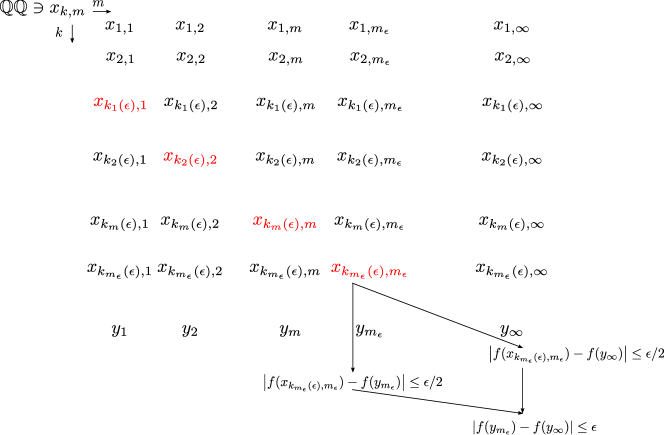
Figure S.4: Illustration of the grid of rational sequences used in the proof of Lemma S.6.9.

S.6.5 Lemmas on asymptotic deterministic equivalents for generalized bias and variance resolvents

In this section, we collect lemmas on asymptotic deterministic equivalents for generalized bias and variance resolvents associated with ridge and ridgeless regression that are used in the proof of Proposition 3.14 in Section S.3, and Proposition 4.10 and Lemma 4.8 in Section S.5.

Lemma S.6.10 (Deterministic equivalents for generalized bias and variance ridge resolvents).

Suppose $X_{i}\in\mathbb{R}^{p}$, $1\leq i\leq n$, are i.i.d. random vectors with each $X_{i}=Z_{i}\Sigma^{1/2}$, where $Z_{i}\in\mathbb{R}^{p}$ contains i.i.d. random variables $Z_{ij}$, $1\leq j\leq p$, each with $\mathbb{E}[Z_{ij}]=0$, $\mathbb{E}[Z_{ij}^{2}]=1$, and $\mathbb{E}[|Z_{ij}|^{8+\alpha}]\leq M_{\alpha}$ for some constants $\alpha>0$ and $M_{\alpha}<\infty$, and $\Sigma\in\mathbb{R}^{p\times p}$ is a positive semidefinite matrix such that $r_{\min}I_{p}\preceq\Sigma\preceq r_{\max}I_{p}$ for some constants $r_{\min}>0$ and $r_{\max}<\infty$ (independent of $p$). Let $\bm{X}\in\mathbb{R}^{n\times p}$ be the random matrix with $X_{i}$, $1\leq i\leq n$, as its rows and let ${\widehat{\bm{\Sigma}}}\in\mathbb{R}^{p\times p}$ denote the $p\times p$ random matrix $\bm{X}^{\top}\bm{X}/n$. Let $A\in\mathbb{R}^{p\times p}$ be any deterministic positive semidefinite matrix that commutes with $\Sigma$ such that $a_{\min}I_{p}\preceq A\preceq a_{\max}I_{p}$ for some constants $a_{\min}>0$ and $a_{\max}<\infty$ (independent of $p$). Let $\gamma_{n}:=p/n$. Then, for $\lambda>0$, as $n,p\to\infty$ with $0<\liminf\gamma_{n}\leq\limsup\gamma_{n}<\infty$, the following asymptotic deterministic equivalences hold:

1. Generalized variance of ridge regression:

   $$({\widehat{\bm{\Sigma}}}+\lambda I_{p})^{-2}{\widehat{\bm{\Sigma}}}A\simeq\widetilde{v}(-\lambda;\gamma_{n})(v(-\lambda;\gamma_{n})\Sigma+I_{p})^{-2}\Sigma A,$$ (E.92)

   where $v(-\lambda;\gamma_{n})\geq 0$ is the unique solution to the fixed-point equation

   $$v(-\lambda;\gamma_{n})^{-1}=\lambda+\gamma_{n}\mathop{\mathrm{tr}}[\Sigma(v(-\lambda;\gamma_{n})\Sigma+I_{p})^{-1}]/p,$$ (E.93)

   and $\widetilde{v}(-\lambda;\gamma_{n})$ is defined via $v(-\lambda;\gamma_{n})$ by the equation

   $$\widetilde{v}(-\lambda;\gamma_{n})^{-1}=v(-\lambda;\gamma_{n})^{-2}-\gamma_{n}\mathop{\mathrm{tr}}[\Sigma^{2}(v(-\lambda;\gamma_{n})\Sigma+I_{p})^{-2}]/p.$$ (E.94)

2. Generalized bias of ridge regression:

   $$\lambda^{2}({\widehat{\bm{\Sigma}}}+\lambda I_{p})^{-1}A({\widehat{\bm{\Sigma}}}+\lambda I_{p})^{-1}\simeq(v(-\lambda;\gamma_{n})\Sigma+I_{p})^{-1}(\widetilde{v}_{g}(-\lambda;\gamma_{n})\Sigma+A)(v(-\lambda;\gamma_{n})\Sigma+I_{p})^{-1},$$ (E.95)

   where $v(-\lambda;\gamma_{n})$ as defined in (E.98), and $\widetilde{v}_{g}(-\lambda;\gamma_{n})$ is defined via $v(-\lambda;\gamma_{n})$ by the equation

   $$\widetilde{v}_{g}(-\lambda;\gamma_{n})=\frac{\displaystyle\gamma_{n}\mathop{\mathrm{tr}}[A\Sigma(v(-\lambda;\gamma_{n})\Sigma+I_{p})^{-2}]/p}{\displaystyle v(-\lambda;\gamma_{n})^{-2}-\gamma_{n}\mathop{\mathrm{tr}}[\Sigma^{2}(v(-\lambda;\gamma_{n})\Sigma+I_{p})^{-2}]/p}.$$ (E.96)

Proof.

The main idea for both the first and second parts is to use Corollary S.7.4 as the starting point, and apply the calculus rules for asymptotic deterministic equivalents listed in Section S.7 to manipulate into the desired equivalents.

Part 1.

For the first part, observe that we can express the resolvent of interest (associated with the generalized variance of ridge regression) as a derivative (with respect to $\lambda$) of a certain resolvent:

$$({\widehat{\bm{\Sigma}}}+\lambda I_{p})^{-2}{\widehat{\bm{\Sigma}}}A=({\widehat{\bm{\Sigma}}}+\lambda I_{p})^{-1}A-\lambda({\widehat{\bm{\Sigma}}}+\lambda I_{p})^{-2}A=\frac{\partial}{\partial\lambda}[\lambda({\widehat{\bm{\Sigma}}}+\lambda I_{p})^{-1}A)].$$ (E.97)

To find a deterministic equivalent for $({\widehat{\bm{\Sigma}}}+\lambda)^{-2}{\widehat{\bm{\Sigma}}}A$, it thus suffices to obtain a deterministic equivalent for the resolvent $\lambda({\widehat{\bm{\Sigma}}}+\lambda I_{p})^{-1}A$ and take its derivative, thanks to the differentiation rule from Lemma S.7.2 (5). Similar derivative trick is used in the proof of Theorem 2.1 in Liu and Dobriban, (2019) and Theorem 2.1 in Dobriban and Wager, (2018) to compute the standard variance of ridge regression, by Dobriban and Sheng, (2020) in the context of distributed ridge regression, and in the earlier works by Karoui and Kösters, (2011); Rubio and Mestre, (2011); Ledoit and Péché, (2011), among others, to compute certain limiting trace functionals.

Starting with Corollary S.7.4, we have

$$\lambda({\widehat{\bm{\Sigma}}}+\lambda I_{p})^{-1}\simeq(v(-\lambda;\gamma_{n})\Sigma+I_{p})^{-1},$$

where $v(-\lambda;\gamma_{n})$ is the unique solution to the fixed point equation

$$v(-\lambda;\gamma_{n})^{-1}=\lambda+\gamma_{n}\mathop{\mathrm{tr}}[\Sigma(v(-\lambda;\gamma_{n})\Sigma+I_{p})^{-1}]/p.$$ (E.98)

Since $A$ has bounded operator norm (uniformly in $p$), from Lemma S.7.2 (3), we have

$$\lambda({\widehat{\bm{\Sigma}}}+\lambda I_{p})^{-1}A\simeq(v(-\lambda;\gamma_{n})\Sigma+I_{p})^{-1}A,$$ (E.99)

where $v(-\lambda;\gamma_{n})$ is as defined by (E.98). It now remains to take the derivative of the right hand side of (E.99) with respect to $\lambda$. Before doing so, we will briefly argue that the differentiation rule indeed applies in this case. Let $T\in\mathbb{R}^{p\times p}$ be a matrix with trace norm uniformly bounded in $p$. Note that

$$\mathop{\mathrm{tr}}[T\lambda({\widehat{\bm{\Sigma}}}+\lambda I_{p})^{-1}A] =\mathop{\mathrm{tr}}[T(I_{p}-{\widehat{\bm{\Sigma}}}({\widehat{\bm{\Sigma}}}+\lambda I_{p})^{-1})A]$$

$$\leq\|(I_{p}-{\widehat{\bm{\Sigma}}}({\widehat{\bm{\Sigma}}}+\lambda I_{p})^{-1})A\|_{\mathrm{op}}\mathop{\mathrm{tr}}[T]$$

$$\leq\|I_{p}-{\widehat{\bm{\Sigma}}}({\widehat{\bm{\Sigma}}}+\lambda I_{p})^{-1}\|_{\mathrm{op}}\|A\|_{\mathrm{op}}\mathop{\mathrm{tr}}[T]$$

$$\leq\|A\|_{\mathrm{op}}\mathop{\mathrm{tr}}[T]\leq C,$$

for some constant $C<\infty$. Here, the first inequality follows from Proposition 3.4.10 of Pedersen, (2012) (see also, Problem III.6.2 of Bhatia, (1997)), and the second inequality follows from the submultiplicativity of the operator norm. Similarly, note that

$$\mathop{\mathrm{tr}}[T(v(-\lambda;\gamma_{n})\Sigma+I_{p})^{-1}A]\leq\|(v(-\lambda;\gamma_{n})\Sigma+I_{p})^{-1}\|_{\mathrm{op}}\|A\|_{\mathrm{op}}\mathop{\mathrm{tr}}[T]\leq C,$$

for some constant $C<\infty$. Thus, we can safely apply the differentiation rule from Lemma S.7.2 (5) to get

$$({\widehat{\bm{\Sigma}}}+\lambda I_{p})^{-1}{\widehat{\bm{\Sigma}}}A\simeq\frac{\partial}{\partial\lambda}[(v(-\lambda;\gamma_{n})\Sigma+I_{p})^{-1}A],$$

we have

$$\frac{\partial}{\partial\lambda}[(v(-\lambda;\gamma_{n})\Sigma+I_{p})^{-1}A]=-\frac{\partial}{\partial\lambda}[v(-\lambda;\gamma_{n})](v(-\lambda;\gamma_{n})\Sigma+I_{p})^{-2}A.$$ (E.100)

We can write - $\partial/\partial\lambda[v(-\lambda;\gamma_{n})]$ in terms of $v(-\lambda;\gamma_{n})$ by taking derivative of (E.98) with respect to $\lambda$ and solving for - $\partial/\partial\lambda[v(-\lambda;\gamma_{n})]$. Taking the derivative of (E.98) yields the following equation:

$$-\frac{\partial}{\partial\lambda}[v(-\lambda;\gamma_{n})]v(-\lambda;\gamma_{n})^{-2}=1+\gamma_{n}-\frac{\partial}{\partial\lambda}[v(-\lambda;\gamma_{n})]\mathop{\mathrm{tr}}[\Sigma^{2}(v(-\lambda;\gamma_{n})\Sigma+I_{p})^{-2}]/p.$$ (E.101)

Denoting - $\partial/\partial\lambda[v(-\lambda;\gamma_{n})]$ by $\widetilde{v}(-\lambda;\gamma_{n})$ and solving for $\widetilde{v}(-\lambda;\gamma_{n})$ in (E.101), we get

$$\widetilde{v}(-\lambda;\gamma_{n})^{-1}=v(-\lambda;\gamma_{n})^{-2}-\gamma_{n}\mathop{\mathrm{tr}}[\Sigma^{2}(v(-\lambda;\gamma_{n})\Sigma+I_{p})^{-2}]/p.$$ (E.102)

Combining (E.97), (E.100), and (E.102), the statement follows. This completes the proof of the first part.

Part 2.

For the second part, observe that we can express the resolvent of interest (appearing in the generalized bias of ridge regression) as a derivative of a certain parameterized resolvent at a fixed value of the parameter:

$$\lambda^{2}({\widehat{\bm{\Sigma}}}+\lambda I_{p})^{-1}A({\widehat{\bm{\Sigma}}}+\lambda I_{p})^{-1}=\lambda^{2}({\widehat{\bm{\Sigma}}}+\lambda I_{p}+\lambda\rho A)^{-1}A({\widehat{\bm{\Sigma}}}+\lambda I_{p}+\lambda\rho A)^{-1}|_{\rho=0}=-\frac{\partial}{\partial\rho}[\lambda({\widehat{\bm{\Sigma}}}+\lambda I_{p}+\lambda\rho A)^{-1}]\mathrel{\Big{|}}_{\rho=0}.$$ (E.103)

It is worth remarking that in contrast to Part 1, we needed to introduce another parameter $\rho$ for this part to appropriately pull out the matrix $A$ in the middle. This trick has been used in the proof of Theorem 5 in Hastie et al., (2019) in the context of standard bias calculation for ridge regression. Our strategy henceforth will be to obtain a deterministic equivalent for the resolvent $\lambda({\widehat{\bm{\Sigma}}}+\lambda I_{p}+\lambda\rho A)^{-1}$, take its derivative with respect to $\rho$, and set $\rho=0$. Towards that end, we first massage it to make it amenable for application of Lemma S.7.3 as follows:

$$\lambda\big{(}{\widehat{\bm{\Sigma}}}+\lambda I_{p}+\lambda\rho A\big{)}^{-1} =\lambda\big{(}{\widehat{\bm{\Sigma}}}+\lambda(I_{p}+\rho A)\big{)}^{-1}$$

$$=(I_{p}+\rho A)^{-1/2}\lambda\big{(}(I_{p}+\rho A)^{-1/2}{\widehat{\bm{\Sigma}}}(I_{p}+\rho\Sigma)^{-1/2}+\lambda I_{p}\big{)}^{-1}(I_{p}+\rho A)^{-1/2}$$

$$=(I_{p}+\rho A)^{-1/2}\lambda\big{(}{\widehat{\bm{\Sigma}}}_{\rho,A}+\lambda I_{p}\big{)}^{-1}(I_{p}+\rho A)^{-1/2},$$ (E.104)

where ${\widehat{\bm{\Sigma}}}_{\rho,A}:=\Sigma_{\rho,A}^{1/2}(\bm{Z}^{\top}\bm{Z}/n)\Sigma_{\rho,A}^{1/2}$ and $\Sigma_{\rho,A}:=(I_{p}+\rho A)^{-1/2}\Sigma(I_{p}+\rho A)^{-1/2}$. We will now obtain a deterministic equivalent for $\lambda({\widehat{\bm{\Sigma}}}_{\rho,A}+\lambda I_{p})^{-1}$, and use the product rule to arrive at the deterministic equivalent for $\lambda({\widehat{\bm{\Sigma}}}+\lambda I_{p}+\lambda\rho A)^{-1}$.

Using Corollary S.7.4, we have

$$\lambda({\widehat{\bm{\Sigma}}}_{\rho,A}+\lambda I_{p})^{-1}\simeq(v_{g}(-\lambda,\rho;\gamma_{n})\Sigma_{\rho,A}+I_{p})^{-1},$$ (E.105)

where $v_{g}(-\lambda,\rho;\gamma_{n})$ is the unique solution to the fixed-point equation

$$v_{g}(-\lambda,\rho;\gamma_{n})^{-1}=\lambda+\gamma_{n}\mathop{\mathrm{tr}}[\Sigma_{\rho,A}(v_{g}(-\lambda,\rho;\gamma_{n})\Sigma_{\rho,A}+I_{p})^{-1}]/p.$$ (E.106)

Combining (E.104) with (E.105), and using the product rule from Lemma S.7.2 (3) (which is applicable since $(I_{p}+\rho A)^{-1/2}$ is a deterministic matrix), we get

$$\lambda({\widehat{\bm{\Sigma}}}+\lambda I_{p}+\lambda\rho A)^{-1} =(I_{p}+\rho A)^{-1/2}\lambda({\widehat{\bm{\Sigma}}}_{\rho,A}+\lambda I_{p})^{-1}(I_{p}+\rho A)^{-1/2}$$

$$\simeq(I_{p}+\rho A)^{-1/2}(v_{g}(-\lambda,\rho;\gamma_{n})\Sigma_{\rho,A}+I_{p})^{-1}(I_{p}+\rho A)^{-1/2}$$

$$=(I_{p}+\rho A)^{-1/2}(v_{g}(-\lambda,\rho;\gamma_{n})(I_{p}+\rho A)^{-1/2}\Sigma(I_{p}+\rho A)^{-1/2}+I_{p})^{-1}(I_{p}+\rho A)^{-1/2}$$

$$=(v_{g}(-\lambda,\rho;\gamma_{n})\Sigma+I_{p}+\rho A)^{-1}.$$

Similarly, the right hand side of the fixed-point equation (E.106) can be simplified by substituting back for $\Sigma_{\rho,A}$ to yield

$$v_{g}(-\lambda,\rho;\gamma_{n})^{-1} =\lambda+\gamma_{n}\mathop{\mathrm{tr}}[(I_{p}+\rho A)^{-1/2}\Sigma(I_{p}+\rho A)^{-1/2}(v_{g}(-\lambda,\rho;\gamma_{n})\Sigma_{\rho,A}+I_{p})^{-1}]/p$$

$$=\lambda+\gamma_{n}\mathop{\mathrm{tr}}[\Sigma(v_{g}(-\lambda,\rho;\gamma_{n})(I_{p}+\rho A)^{1/2}\Sigma_{\rho,A}(I_{p}+\rho A)^{1/2}+(I_{p}+\rho A))^{-1}]/p$$

$$=\lambda+\gamma_{n}\mathop{\mathrm{tr}}[\Sigma(v_{g}(-\lambda,\rho;\gamma_{n})\Sigma+I_{p}+\rho A)^{-1}]/p.$$ (E.107)

Finally, we will now use the differentiation rule from Lemma S.7.2 (5) (with respect to $\rho$ this time). The applicability of the differentiation rule follows analogously to first part for $\rho>-1/a_{\min}$. Additionally, it is easy to verify that both sides of (E.107) are analytic in $\rho$. Taking derivative with respect to $\rho$, we get

$$-\frac{\partial}{\partial\rho}[(v_{g}(-\lambda,\rho;\gamma_{n})\Sigma+I_{p}+\rho A)^{-1}]=(v_{g}(-\lambda,\rho;\gamma_{n})\Sigma+I_{p}+\rho A)^{-1}\left(\frac{\partial}{\partial\rho}[v_{g}(-\lambda,\rho;\gamma_{n})]\Sigma+A\right)(v_{g}(-\lambda,\rho;\gamma_{n})\Sigma+I_{p}+\rho A)^{-1}.$$ (E.108)

Setting $\rho=0$ and observing that $v_{g}(-\lambda,0;\gamma_{n})=v(-\lambda;\gamma_{n})$, where $v(-\lambda;\gamma_{n})$ is as defined in (E.98), we have

$$\frac{\partial}{\partial\rho}[(v_{g}(-\lambda,\rho;\gamma_{n})\Sigma+I_{p}+\rho A)^{-1}]\mathrel{\Big{|}}_{\rho=0}=(v(-\lambda;\gamma_{n})\Sigma+I_{p})^{-1}\left(\frac{\partial}{\partial\rho}[v_{g}(-\lambda,\rho;\gamma_{n})]\mathrel{\Big{|}}_{\rho=0}\Sigma+A\right)(v(-\lambda;\gamma_{n})\Sigma+I_{p})^{-1}.$$ (E.109)

To obtain an equation for $\partial/\partial\rho[v_{g}(-\lambda,\rho;\gamma_{n})]|_{\rho=0}$, we can differentiate the fixed-point equation (E.107) with respect to $\rho$ to yield

$$-\frac{\partial}{\partial\rho}[v_{g}(-\lambda,\rho;\gamma_{n})]v_{g}(-\lambda,\rho;\gamma_{n})^{-2}=-\gamma_{n}\frac{\partial}{\partial\rho}[v_{g}(-\lambda,\rho;\gamma_{n})]\mathop{\mathrm{tr}}[\Sigma^{2}(v_{g}(-\lambda,\rho;\gamma_{n})\Sigma+I_{p}+\rho A)^{-2}]/p\\ -\gamma_{n}\mathop{\mathrm{tr}}[A\Sigma(v_{g}(-\lambda,\rho;\gamma_{n})\Sigma+I_{p}+\rho A)^{-2}]/p.$$ (E.110)

Setting $\rho=0$ in the equation above, and using the fact that $v_{g}(-\lambda,0;\gamma_{n})=v(-\lambda;\gamma_{n})$, and denoting $\partial/\partial\rho[v_{g}(-\lambda,\rho;\gamma_{n})]|_{\rho=0}$ by $\widetilde{v}_{g}(-\lambda;\gamma_{n})$, we get that

$$\widetilde{v}_{g}(-\lambda;\gamma_{n})=\frac{\displaystyle\gamma_{n}\mathop{\mathrm{tr}}[A\Sigma(v(-\lambda;\gamma_{n})\Sigma+I_{p})^{-2}]/p}{\displaystyle v(-\lambda;\gamma_{n})^{-2}-\gamma_{n}\mathop{\mathrm{tr}}[\Sigma^{2}(v(-\lambda;\gamma_{n})\Sigma+I_{p})^{-2}]/p}.$$ (E.111)

Therefore, from (E.103) and (E.109), we finally have

$$\lambda^{2}({\widehat{\bm{\Sigma}}}+\lambda I_{p})^{-1}A({\widehat{\bm{\Sigma}}}+\lambda I_{p})^{-1}\simeq(v(-\lambda;\gamma_{n})\Sigma+I_{p})^{-1}(\widetilde{v}_{g}(-\lambda;\gamma_{n})\Sigma+A)(v(-\lambda;\gamma_{n})\Sigma+I_{p})^{-1},$$

where $v(-\lambda;\gamma_{n})$ is as defined in (E.98), and $\widetilde{v}_{g}(-\lambda;\gamma_{n})$ is as defined in (E.111). This completes the proof of the second part.

∎

Lemma S.6.11 (Deterministic equivalents for generalized bias and variance ridgeless resolvents).

Assume the setting of Lemma S.6.10 with $\gamma_{n}\in(1,\infty)$. Then, the following deterministic equivalences hold:

1. Generalized variance of ridgeless regression:

   $${\widehat{\bm{\Sigma}}}^{+}A\simeq\widetilde{v}(0;\gamma_{n})(v(0;\gamma_{n})\Sigma+I_{p})^{-2}\Sigma A,$$ (E.112)

   where $v(0;\gamma_{n})$ is the unique solution to the fixed-point equation

   $$\gamma_{n}^{-1}=\mathop{\mathrm{tr}}[v(0;\gamma_{n})\Sigma(v(0;\gamma_{n})\Sigma+I_{p})^{-1}]/p,$$ (E.113)

   and $\widetilde{v}(0;\gamma_{n})$ is defined through $v(0;\gamma_{n})$ via

   $$\widetilde{v}(0;\gamma_{n})=\big{(}v(0;\gamma_{n})^{-2}-\gamma_{n}\mathop{\mathrm{tr}}[\Sigma^{2}(v(0;\gamma_{n})\Sigma+I_{p})^{-2}]/p\big{)}^{-1}.$$ (E.114)

2. Generalized bias of ridgeless regression:

   $$(I_{p}-{\widehat{\bm{\Sigma}}}^{+}{\widehat{\bm{\Sigma}}})A(I_{p}-{\widehat{\bm{\Sigma}}}^{+}{\widehat{\bm{\Sigma}}})\simeq(v(0;\gamma_{n})\Sigma+I_{p})^{-1}(\widetilde{v}_{g}(0;\gamma_{n})\Sigma+A)(v(0;\gamma_{n})\Sigma+I_{p})^{-1},$$ (E.115)

where $v(0;\gamma_{n})$ is as defined in (E.113), and $\widetilde{v}_{g}(0;\gamma_{n})$ is defined via $v(0;\gamma_{n})$ by

$$\widetilde{v}_{g}(0;\gamma_{n})=\gamma_{n}\mathop{\mathrm{tr}}[A\Sigma(v(0;\gamma_{n})\Sigma+I_{p})^{-2}]/p\cdot\big{(}v(0;\gamma_{n})^{-2}-\gamma_{n}\mathop{\mathrm{tr}}[\Sigma^{2}(v(0;\gamma_{n})\Sigma+I_{p})^{-2}]/p\big{)}^{-1}.$$ (E.116)

Proof.

The proofs for both the parts use the results of Lemma S.6.10 and a limiting argument as $\lambda\to 0^{+}$. The results of Lemma S.6.10 are pointwise in $\lambda$, but can be strengthened to be uniform in $\lambda$ over a range that includes $\lambda=0$ allowing one to take the limits of the deterministic equivalents obtained in Lemma S.6.10 as $\lambda\to 0^{+}$.

Part 1.

We will use the result in Part 1 of Lemma S.6.10 as our starting point. Let $\Lambda:=[0,\lambda_{\max}]$ where $\lambda_{\max}<\infty$, and let $T$ be a matrix with bounded trace norm. Note that

$$|\mathop{\mathrm{tr}}[({\widehat{\bm{\Sigma}}}+\lambda I_{p})^{-2}{\widehat{\bm{\Sigma}}}AT]|\leq\|({\widehat{\bm{\Sigma}}}+\lambda I_{p})^{-2}{\widehat{\bm{\Sigma}}}A\|_{\mathrm{op}}\mathop{\mathrm{tr}}[T]\leq C\|({\widehat{\bm{\Sigma}}}+\lambda I_{p})^{-2}{\widehat{\bm{\Sigma}}}\|_{\mathrm{op}}\|A\|_{\mathrm{op}}\leq C$$ (E.117)

for some constant $C<\infty$. Here, the last inequality follows because $s_{i}^{2}/(s_{i}^{2}+\lambda)^{2}\leq 1$ where $s_{i}^{2}$, $1\leq i\leq p$, are the eigenvalues of ${\widehat{\bm{\Sigma}}}$, and the operator norm $A$ is assumed to be bounded. Consider the magnitude of the derivative (in $\lambda$) of the map $\lambda\mapsto\mathop{\mathrm{tr}}[({\widehat{\bm{\Sigma}}}+\lambda I_{p})^{-2}{\widehat{\bm{\Sigma}}}AT]$ given by

$$\left|\frac{\partial}{\partial\lambda}\mathop{\mathrm{tr}}[({\widehat{\bm{\Sigma}}}+\lambda I_{p})^{-2}{\widehat{\bm{\Sigma}}}AT]\right|=2|\mathop{\mathrm{tr}}[({\widehat{\bm{\Sigma}}}+\lambda I_{p})^{-3}{\widehat{\bm{\Sigma}}}AT]|.$$

Following the argument in (E.117), for $\lambda\in\Lambda$, observe that

$$|\mathop{\mathrm{tr}}[({\widehat{\bm{\Sigma}}}+\lambda I_{p})^{-3}{\widehat{\bm{\Sigma}}}AT]|\leq\|({\widehat{\bm{\Sigma}}}+\lambda I_{p})^{-3}{\widehat{\bm{\Sigma}}}\|_{\mathrm{op}}\|A\|_{\mathrm{op}}\mathop{\mathrm{tr}}[T]\leq C$$

for some constant $C<\infty$. Similarly, in the same interval $\mathop{\mathrm{tr}}[\widetilde{v}(-\lambda;\gamma_{n})(v(-\lambda;\gamma_{n})\Sigma+I_{p})^{-2}\Sigma AT]\leq C.$ In addition, from Lemma S.6.14, we have the map $\lambda\mapsto\mathop{\mathrm{tr}}[\widetilde{v}(-\lambda;\gamma_{n})(v(-\lambda;\gamma_{n})\Sigma+I_{p})^{-2}AT]$ is differentiable in $\lambda$ and the derivative for $\lambda\in\Lambda$ is bounded. Therefore, the family of functions $\mathop{\mathrm{tr}}[({\widehat{\bm{\Sigma}}}+\lambda I_{p})^{-2}{\widehat{\bm{\Sigma}}}AT]-\mathop{\mathrm{tr}}[\widetilde{v}(-\lambda;\gamma_{n})(v(-\lambda;\gamma_{n})\Sigma+I_{p})^{-2}\Sigma AT]$ forms an equicontinuous family in $\lambda$ over $\lambda\in\Lambda$. Thus, the convergence in Part 1 of Lemma S.6.10 is uniforms in $\lambda$. We can now use the Moore-Osgood theorem to interchange the limits to obtain

$$\lim_{p\to\infty}\mathop{\mathrm{tr}}[{\widehat{\bm{\Sigma}}}^{+}AT]-\mathop{\mathrm{tr}}[\widetilde{v}(0;\gamma_{n})(v(0;\gamma_{n})\Sigma+I_{p})^{-2}\Sigma AT]$$

$$=\lim_{p\to\infty}\lim_{\lambda\to 0^{+}}\mathop{\mathrm{tr}}[({\widehat{\bm{\Sigma}}}+\lambda I_{p})^{-2}{\widehat{\bm{\Sigma}}}AT]-\mathop{\mathrm{tr}}[\widetilde{v}(-\lambda;\gamma_{n})(v(-\lambda;\gamma_{n})\Sigma+I_{p})^{-2}\Sigma AT)]$$

$$=\lim_{\lambda\to 0^{+}}\lim_{p\to\infty}\mathop{\mathrm{tr}}[({\widehat{\bm{\Sigma}}}+\lambda I_{p})^{-2}{\widehat{\bm{\Sigma}}}AT]-\mathop{\mathrm{tr}}[\widetilde{v}(-\lambda;\gamma_{n})(v(-\lambda;\gamma_{n})\Sigma+I_{p})^{-2}\Sigma AT)]$$

$$=0.$$

In the first equality above, we used the fact that ${\widehat{\bm{\Sigma}}}^{+}={\widehat{\bm{\Sigma}}}^{+}{\widehat{\bm{\Sigma}}}{\widehat{\bm{\Sigma}}}^{+}=\lim_{\lambda\to 0^{+}}({\widehat{\bm{\Sigma}}}+\lambda I_{p})^{-1}{\widehat{\bm{\Sigma}}}({\widehat{\bm{\Sigma}}}+\lambda I_{p})^{-1}$, and that the functions $v(\cdot;\gamma_{n})$ and $\widetilde{v}(\cdot;\gamma_{n})$ are continuous (which follows, from say Lemma S.6.15 (1)). This provides the right hand side of (E.112). Similarly, the fixed-point equation (E.98) as $\lambda\to 0^{+}$ becomes

$$v(0;\gamma_{n})^{-1}=\gamma_{n}\mathop{\mathrm{tr}}[\Sigma(v(0;\gamma_{n})\Sigma+I_{p})^{-1}]/p.$$

Moving $v(0;\gamma_{n})$ to the other side (from Lemma S.6.13 (1), it follows that $v(0;\gamma_{n})>0$ for $\gamma_{n}\in(1,\infty)$), we arrive at the desired result.

Part 2.

As done in Part 1, it is not difficult to show that over $\lambda\in\Lambda$ the family of functions $\mathop{\mathrm{tr}}[\lambda^{2}({\widehat{\bm{\Sigma}}}+\lambda I_{p})^{-1}A({\widehat{\bm{\Sigma}}}+\lambda I_{p})^{-1}T]-\mathop{\mathrm{tr}}[(v(-\lambda;\gamma_{n})\Sigma+I_{p})^{-1}(\widetilde{v}_{g}(-\lambda;\gamma_{n})\Sigma+A)(v(-\lambda;\gamma_{n})\Sigma+I_{p})^{-1}T]$ form an equicontinuous family. Therefore, the convergence in Part 2 of Lemma S.6.10 is uniform in $\lambda$ over $\Lambda$ (that includes $0$). Using the Moore-Osgood theorem to the interchange the limits, one has

$$\lim_{p\to\infty}\mathop{\mathrm{tr}}[(I_{p}-{\widehat{\bm{\Sigma}}}^{+}{\widehat{\bm{\Sigma}}})A(I_{p}-{\widehat{\bm{\Sigma}}}^{+}{\widehat{\bm{\Sigma}}})T]-\mathop{\mathrm{tr}}[(v(0;\gamma_{n})\Sigma+I_{p})^{-1}(\widetilde{v}_{g}(0;\gamma_{n})\Sigma+A)(v(0;\gamma_{n})\Sigma+I_{p})^{-1}T]$$

$$=\lim_{p\to\infty}\lim_{\lambda\to 0^{+}}\mathop{\mathrm{tr}}[\lambda^{2}({\widehat{\bm{\Sigma}}}+\lambda I_{p})^{-1}A({\widehat{\bm{\Sigma}}}+\lambda I_{p})^{-1}T]-\mathop{\mathrm{tr}}[(v(-\lambda;\gamma_{n})\Sigma+I_{p})^{-1}(\widetilde{v}_{g}(-\lambda;\gamma_{n})\Sigma+A)(v(-\lambda;\gamma_{n})\Sigma+I_{p})^{-1}T]$$

$$=\lim_{\lambda\to 0^{+}}\lim_{p\to\infty}\mathop{\mathrm{tr}}[\lambda^{2}({\widehat{\bm{\Sigma}}}+\lambda I_{p})^{-1}A({\widehat{\bm{\Sigma}}}+\lambda I_{p})^{-1}T]-\mathop{\mathrm{tr}}[(v(-\lambda;\gamma_{n})\Sigma+I_{p})^{-1}(\widetilde{v}_{g}(-\lambda;\gamma_{n})\Sigma+A)(v(-\lambda;\gamma_{n})\Sigma+I_{p})^{-1}T]$$

$$=0.$$

Now both (E.114) and (E.116) follow by taking $\lambda\to 0^{+}$ in (E.95) and (E.96), respectively.

This concludes the proof.

∎

Corollary S.6.12 (Limiting deterministic equivalents for generalized bias and variance ridgeless resolvents).

Assume the setting of Lemma S.6.10. Let $f:\mathbb{R}_{\geq 0}\to\mathbb{R}_{\geq 0}$ be a function. Then, as $n,p\to\infty$ and $p/n\to\gamma\in(1,\infty)$, the following equivalences hold:

1. Limiting generalized variance of ridgeless regression:

   $${\widehat{\bm{\Sigma}}}^{+}f(\Sigma)\simeq\widetilde{v}(0;\gamma)(v(0;\gamma)\Sigma+I_{p})^{-2}\Sigma f(\Sigma),$$ (E.118)

   where $v(0;\gamma)$ and $\widetilde{v}(0;\gamma)$ are defined by (E.113) and (E.114), respectively.

2. Limiting generalized bias of ridgeless regression:

   $$(I_{p}-{\widehat{\bm{\Sigma}}}^{+}{\widehat{\bm{\Sigma}}})f(\Sigma)(I_{p}-{\widehat{\bm{\Sigma}}}^{+}{\widehat{\bm{\Sigma}}})\simeq(1+\widetilde{v}_{g}(0;\gamma))(v(0;\gamma)\Sigma+I_{p})^{-1}f(\Sigma)(v(0;\gamma)\Sigma+I_{p})^{-1},$$ (E.119)

   where $v(0;\gamma)$ is as defined in (E.113) and $\widetilde{v}_{g}(0;\gamma)$ is as defined in (E.116) with $A$ replaced by $f(\Sigma)$.

Proof.

The proof follows from Lemma S.6.11, in conjunction with Lemma S.6.13 ((1), (3), (4)) to provide continuity of the functions $v(0;\cdot)$, $\widetilde{v}(0;\cdot)$, and $\widetilde{v}_{g}(0;\cdot)$ (in the aspect ratio) over $(1,\infty)$. ∎

S.6.6 Lemmas on properties of solutions of certain fixed-point equations

In this section, we collect helper lemmas that are used in the proofs of Proposition 3.14 in Section S.3, Corollary 4.9 in Section S.5, and Lemma S.6.11 and Corollary S.6.12 in Section S.6.

Lemma S.6.13 (Continuity and limiting behavior of functions of the solution of a fixed-point equation in the aspect ratio).

Let $a>0$ and $b<\infty$ be real numbers. Let $P$ be a probability measure supported on $[a,b]$. Consider the function $v(0;\cdot):\phi\mapsto v(0;\phi)$, over $(1,\infty)$, where $v(0;\phi)\geq 0$ is the unique solution to the fixed-point equation

$$\frac{1}{\phi}=\int\frac{v(0;\phi)r}{1+v(0;\phi)r}\,\mathrm{d}P(r).$$ (E.120)

Then, the following properties hold:

1. The function $v(0;\cdot)$ is continuous and strictly decreasing over $(1,\infty)$. Furthermore, $\lim_{\phi\to 1^{+}}v(0;\phi)=\infty$, and $\lim_{\phi\to\infty}v(0;\phi)=0$.

2. The function $\phi\mapsto(\phi v(0;\phi))^{-1}$ is strictly increasing over $(1,\infty)$. Furthermore, $\lim_{\phi\to 1^{+}}(\phi v(0;\phi))^{-1}=0$ and $\lim_{\phi\to\infty}(\phi v(0;\phi))^{-1}=1$.

3. The function $\widetilde{v}(0;\cdot):\phi\mapsto\widetilde{v}(0;\phi)$, where

   $$\widetilde{v}(0;\phi)=\left(\frac{1}{v(0;\phi)^{2}}-\phi\int\frac{r^{2}}{(1+rv(0;\phi))^{2}}\,\mathrm{d}P(r)\right)^{-1},$$

   is continuous over $(1,\infty)$. Furthermore, $\lim_{\phi\to 1^{+}}\widetilde{v}(0;\phi)=\infty$, and $\lim_{\phi\to\infty}\widetilde{v}(0;\phi)=0$.

4. The function $\widetilde{v}_{g}(0;\cdot):\phi\mapsto\widetilde{v}_{g}(0;\phi)$, where

   $$\widetilde{v}_{g}(0;\phi)=\widetilde{v}(0;\phi)\phi\int\frac{r^{2}}{(1+v(0;\phi)r)^{2}}\,\mathrm{d}P(r),$$

   is continuous over $(1,\infty)$. Furthermore, $\lim_{\phi\to 1^{+}}\widetilde{v}_{g}(0;\phi)=\infty$, and $\lim_{\phi\to\infty}\widetilde{v}_{g}(0;\phi)=0$.

5. Let $Q$ be a (fixed) probability distribution supported on $[a,b]$ that depends on a scalar $\phi_{1}$. Then, the function $\Upsilon_{b}(\phi_{1};\cdot):\phi\mapsto\Upsilon_{b}(\phi_{1},\phi)$, where

   $$\Upsilon_{b}(\phi_{1},\phi)=(1+\widetilde{v}_{g}(0;\phi))\int\frac{1}{(1+v(0;\phi)r)^{2}}\,\mathrm{d}Q(r),$$

   is continuous over $(1,\infty)$. Furthermore, $\Upsilon_{b}(\phi_{1},\phi)<\infty$ for $\phi\in(1,\infty)$, and $\lim_{\phi\to\infty}\Upsilon_{b}(\phi_{1},\phi)=1$.

Proof.

We consider the five parts separately below. Before doing so though, it is worth mentioning that for $\phi\in(1,\infty)$, there is a unique non-negative solution $v(0;\phi)$ to the fixed-point equation (E.120) as stated in the statement. This follows from Lemma S.6.15 (1). The following properties refer to the function $v(0;\cdot):\phi\mapsto v(0;\phi)$ defined via this unique solution.

Part 1.

We begin with the first part. Observe that the function

$$t\mapsto\int\frac{1}{1+tr}\,\mathrm{d}P(r)$$

is strictly decreasing and strictly convex over $(0,\infty)$. Thus, the function

$$T:t\mapsto 1-\int\frac{1}{1+tr}\,\mathrm{d}P(r)=\int\frac{t}{1+tr}\,\mathrm{d}P(r)$$

is strictly increasing and strictly concave over $(0,\infty)$, with $\lim_{t\to 0}T(t)=0$ and $\lim_{t\to\infty}T(t)=1$. Since the inverse image of a strictly increasing and strictly concave real function is strictly increasing and strictly convex (see, e.g. Proposition 3 of Hiriart-Urruty and Martınez-Legaz, (2003)), we have that $T^{-1}$ is strictly convex and strictly increasing. This also implies that $T^{-1}$ is continuous. Note that $v(0;\phi)=T^{-1}(\phi^{-1})$. Since $\phi^{-1}$ is continuous, it follows that $v(0;\cdot)$ is continuous. In addition, since $\phi\mapsto\phi^{-1}$ is strictly decreasing, we have that $v(0;\cdot)$ is strictly decreasing. Moreover, $\lim_{\phi\to 1^{+}}T^{-1}(\phi^{-1})=\infty$, and $\lim_{\phi\to\infty}T^{-1}(\phi^{-1})=0$.

Part 2.

From (E.120), we have

$$\frac{1}{\phi v(0;\phi)}=\int\frac{r}{1+v(0;\phi)r}\,\mathrm{d}P(r).$$

Because $v(0;\phi)$ is strictly decreasing over $(1,\infty)$, the right side of the display above is strictly increasing. Furthermore, because $\lim_{\phi\to 1^{+}}v(0;\phi)=\infty$, we have $\lim_{\phi\to 1^{+}}(\phi v(0;\phi))^{-1}=0$, and because $\lim_{\phi\to\infty}v(0;\phi)=0$, we have $\lim_{\phi\to\infty}(\phi v(0;\phi))^{-1}=1$.

Part 3.

From Part 1, the function $1/v(0;\cdot)^{2}$ is continuous. In addition, observe that the function

$$\phi\mapsto\int\frac{r^{2}}{(1+v(0;\phi)r)^{2}}\,\mathrm{d}P(r)$$

is also continuous. Thus, $\widetilde{v}(0;\cdot)$ is continuous. Furthermore, since $\lim_{\phi\to 1^{+}}v(0;\phi)=\infty$, it follows that $\lim_{\phi\to 1^{+}}\widetilde{v}(0;\phi)=\infty$. Similarly, from $\lim_{\phi\to\infty}v(0;\phi)=0$ and the fact that

$$\lim_{\phi\to\infty}\int\frac{r^{2}}{(1+rv(0;\phi))^{2}}\,\mathrm{d}P(r)\geq a^{2}>0,$$

it follows that $\lim_{\phi\to\infty}\widetilde{v}(0;\phi)=0$.

Part 4.

Similar to Part 3, continuity of $\widetilde{v}_{g}(0;\cdot)$ follows from the continuity of $\widetilde{v}(0;\cdot)$ and $v(0;\phi)$. To compute the desired limits, observe that

$$1+\widetilde{v}_{g}(0;\phi)=\frac{\displaystyle\frac{1}{v(0;\phi)^{2}}}{\displaystyle\frac{1}{v(0;\phi)^{2}}-\phi\int\frac{r^{2}}{(1+v(0;\phi)r)^{2}}\,\mathrm{d}P(r)}.$$

We thus have

$$(1+\widetilde{v}_{g}(0;\phi))^{-1} =1-v(0;\phi)^{2}\phi\int\frac{r^{2}}{(1+rv(0;\phi))^{2}}\,\mathrm{d}P(r)$$ (E.121)

$$=1-\phi\int\frac{r^{2}}{(v(0;\phi)^{-1}+r)^{2}}\,\mathrm{d}P(r).$$ (E.122)

Because $\lim_{\phi\to 1^{+}}v(0;\phi)=\infty$, from (E.122), we have

$$\lim_{\phi\to 1^{+}}(1+\widetilde{v}_{g}(0;\phi))^{-1}=1-\lim_{\phi\to 1^{+}}\phi\int\frac{r^{2}}{(v(0;\phi)^{-1}+r)^{2}}\mathrm{d}P(r)=1-1=0.$$

It follows then that $\lim_{\phi\to 1^{+}}\widetilde{v}_{g}(0;\phi)=\infty$.

On the other hand, observe from (E.121) that

$$(1+\widetilde{v}_{g}(0;\phi))^{-1}=1-\phi v(0;\phi)v(0;\phi)\int\frac{r^{2}}{(1+rv(0;\phi))^{2}}\,\mathrm{d}P(r).$$ (E.123)

From Part 2, we have $\lim_{\phi\to\infty}\phi v(0;\phi)=1$, and from Part 1, we have $\lim_{\phi\to\infty}v(0;\phi)=0$. Moreover, since $P$ is supported on $[a,b]$, and $v(0;\phi)>0$ for $\phi\in(1,\infty)$ from Part 1, for $\phi\in(1,\infty)$, note that

$$0<\int\frac{r^{2}}{(1+rv(0;\phi))^{2}}<b^{2}.$$

Thus, from (E.123), we obtain

$$\lim_{\phi\to\infty}(1+\widetilde{v}_{g}(0;\phi))^{-1}=1-0=1.$$

We hence conclude that $\lim_{\phi\to\infty}\widetilde{v}_{g}(0;\phi)=0$.

Part 5.

The continuity claim follows from the continuity of $v(0;\cdot)$ and $\widetilde{v}_{g}(0;\cdot)$ from Parts 1 and 4, respectively. From calculation similar to that in Part 4, it follows that $(1+\widetilde{v}_{g}(0;\phi))<\infty$ for $\phi\in(1,\infty)$. Now, since $v(0;\phi)>0$ for $\phi\in(1,\infty)$ from Part 1, and $Q$ is supported on $[a,b]$, observe that

$$\int\frac{1}{(1+v(0;\phi)r)^{2}}\,\mathrm{d}Q(r)\leq 1<\infty.$$

Hence, $\Upsilon_{b}(\phi_{1},\phi)<\infty$ for $\phi\in(1,\infty)$. Moreover, because $\lim_{\phi\to\infty}(1+\widetilde{v}_{g}(0;\phi))=1$, and $\lim_{\phi\to\infty}v(0;\phi)=0$, we obtain

$$\lim_{\phi\to\infty}\Upsilon_{b}(\phi_{1},\phi)=\lim_{\phi\to\infty}(1+\widetilde{v}_{g}(0;\phi))\cdot\lim_{\phi\to\infty}\int\frac{1}{(1+v(0;\phi)r)^{2}}\,\mathrm{d}Q(r)=1.$$

Therefore, $\lim_{\phi\to\infty}\Upsilon_{b}(\phi_{1},\phi)=1$, as desired.

This completes all the five parts, and finishes the proof. ∎

Lemma S.6.14 (Bounding derivatives of the solution of a fixed-point equation in the regularization parameter).

Let $a>0$ and $b<0$ be real numbers. Let $P$ be a probability measure supported on $[a,b]$. Let $\gamma\in(1,\infty)$ be a real number. Let $\Lambda=[0,\lambda_{\max}]$ for some constant $\lambda_{\max}<\infty$. For $\lambda\in\Lambda$, let $v(-\lambda;\gamma)\geq 0$ denote the solution to the fixed-point equation

$$\frac{1}{v(-\lambda;\gamma)}=\lambda+\gamma\int\frac{r}{v(-\lambda;\gamma)r+1}\,\mathrm{d}P(r).$$

Then, the function $\lambda\mapsto v(-\lambda;\gamma)$ is twice differentiable over $\Lambda$. Furthermore, over $\Lambda$, $v(-\lambda;\gamma)$, $\partial/\partial\lambda[v(-\lambda;\gamma)]$, and $\partial^{2}/\partial\lambda^{2}[v(-\lambda;\gamma)]$ are bounded above.

Proof.

Start by re-writing the fixed-point equation as

$$\lambda=\frac{1}{v(-\lambda;\gamma)}-\gamma\int\frac{r}{v(-\lambda;\gamma)r+1}\,\mathrm{d}P(r).$$

Define a function $f$ by

$$f(x)=\frac{1}{x}-\gamma\int\frac{r}{xr+1}\,\mathrm{d}P(r).$$

Observe that $v(-\lambda;\gamma)=f^{-1}(\lambda)$. The claim of twice differentiability of the function $\lambda\mapsto v(-\lambda;\gamma_{n})$ follows from Lemma S.6.15 (4). The claim of boundedness of the function and its first derivatives (with respect to $\lambda$) follows from Lemma S.6.15 ((4), (5), (6)).

∎

Lemma S.6.15 (Bounding derivatives of the solution of a fixed-point equation).

Let $a>0$ and $b<\infty$ be two real numbers. Let $P$ be a probability distribution supported on $[a,b]$. Let $\gamma\in(1,\infty)$ be a real number. Define a function $f$ by

$$f(x)=\frac{1}{x}-\gamma\int\frac{r}{xr+1}\,\mathrm{d}P(r).$$ (E.124)

Then, the following properties hold:

1. There is a unique $0<x_{0}<\infty$ such that $f(x_{0})=0$. The function $f$ is twice differentiable and strictly decreasing over $(0,x_{0})$, with $\lim_{x\to 0^{+}}f(x)=\infty$ and $f(x_{0})=0$.

2. The derivative $f^{\prime}$ is strictly increasing over $(0,x_{0})$, with $\lim_{x\to 0^{+}}f^{\prime}(x)=-\infty$ and $f^{\prime}(x_{0})<0$.

3. The second derivative $f^{\prime\prime}$ is strictly decreasing over $(0,x_{0})$, with $\lim_{x\to 0^{+}}f^{\prime\prime}(x)=\infty$ and $f^{\prime\prime}(x_{0})>0$.

4. The inverse function $f^{-1}$ is twice differentiable, bounded over $[0,\infty)$ by $x_{0}<\infty$, and strictly decreasing over $(0,\infty)$, with $f^{-1}(0)=x_{0}$ and $\lim_{y\to\infty}f^{-1}(y)=0$.

5. The derivative of the inverse function $(f^{-1})^{\prime}$ is bounded over $[0,\infty)$ by

   $$\frac{\displaystyle x_{0}^{2}}{\displaystyle 1-\gamma\int\left(\frac{x_{0}r}{x_{0}r+1}\right)^{2}\,\mathrm{d}P(r)}<\infty.$$

6. The second derivative of the inverse function $(f^{-1})^{\prime\prime}$ is bounded over $[0,\infty)$ by

   $$\frac{\displaystyle 2x_{0}^{3}}{\displaystyle\left(1-\gamma\int\left(\frac{x_{0}r}{x_{0}r+1}\right)^{2}\,\mathrm{d}P(r)\right)^{3}}<\infty.$$

Proof.

We consider different parts separately below.

Part 1.

Observe that

$$f(x)=\frac{1}{x}-\gamma\int\frac{r}{xr+1}\,\mathrm{d}P(r)=\frac{1}{x}\left(1-\gamma\int\frac{xr}{xr+1}\,\mathrm{d}P(r)\right).$$

The function $g:x\mapsto 1/x$ is positive and strictly decreasing over $(0,\infty)$ with $\lim_{x\to 0^{+}}g(x)=\infty$ and $\lim_{x\to\infty}g(x)=0$, while the function

$$h:x\mapsto 1-\gamma\int\frac{xr}{xr+1}\,\mathrm{d}P(r)$$

is strictly decreasing over $(0,\infty)$ with $h(0)=1$ and $\lim_{x\to\infty}h(x)=1-\gamma<0$. Thus, there is a unique $0<x_{0}<\infty$ such that $h(x_{0})=0$, and consequently $f(x_{0})=0$. Because $h$ is positive over $[0,x_{0}]$, $f$, a product of two positive strictly decreasing functions, is strictly decreasing over $(0,x_{0})$, with $\lim_{x\to 0^{+}}f(x)=\infty$ and $f(x_{0})=0$.

Part 2.

The derivative $f^{\prime}$ at $x$ is given by

$$f^{\prime}(x)=-\frac{1}{x^{2}}+\gamma\int\frac{r^{2}}{(xr+1)^{2}}\,\mathrm{d}P(r)=-\frac{1}{x^{2}}\left(1-\gamma\int\left(\frac{xr}{xr+1}\right)^{2}\,\mathrm{d}P(r)\right).$$

The function $g:x\mapsto 1/x^{2}$ is positive and strictly decreasing over $(0,\infty)$ with $\lim_{x\to 0^{+}}g(x)=\infty$ and $\lim_{x\to\infty}g(x)=0$. On the other hand, the function

$$h:x\mapsto 1-\gamma\int\left(\frac{xr}{xr+1}\right)^{2}\,\mathrm{d}P(r)$$

strictly decreasing over $(0,\infty)$ with $h(0)=1$ and $h(x_{0})>0$. This follows because for $x\in[0,x_{0}]$,

$$\begin{split}\gamma\int\left(\frac{xr}{xr+1}\right)^{2}\,\mathrm{d}P(r)&\leq\left(\frac{x_{0}b}{x_{0}b+1}\right)\gamma\int\left(\frac{xr}{xr+1}\right)\,\mathrm{d}P(r)\\ &<\gamma\int\frac{xr}{xr+1}\,\mathrm{d}P(r)\leq\gamma\int\frac{x_{0}r}{x_{0}r+1}\,\mathrm{d}P(r)=1,\end{split}$$ (E.125)

where the first inequality in the chain above follows as the support of $P$ is $[a,b]$, and the last inequality follows since $f(x_{0})=0$ and $x_{0}>0$, which implies that

$$\frac{1}{x_{0}}=\gamma\int\frac{r}{x_{0}r+1}\,\mathrm{d}P(r),\quad\text{ or equivalently that}\quad 1=\gamma\int\frac{x_{0}r}{x_{0}r+1}\,\mathrm{d}P(r).$$

Thus, $-f^{\prime}$, a product of two positive strictly decreasing functions, is strictly decreasing, and in turn, $f^{\prime}$ is strictly increasing. Moreover, $\lim_{x\to 0^{+}}f^{\prime}(x)=-\infty$ and $f^{\prime}(x_{0})<0$.

Part 3.

The second derivative $f^{\prime\prime}$ at $x$ is given by

$$f^{\prime\prime}(x)=\frac{2}{x^{3}}-2\gamma\int\frac{r^{3}}{(xr+1)^{3}}\,\mathrm{d}P(r)=\frac{2}{x^{3}}\left(1-\gamma\int\left(\frac{xr}{xr+1}\right)^{3}\,\mathrm{d}P(r)\right).$$

The rest of the arguments are similar to those in Part 2. The function $g:x\mapsto 1/x^{3}$ is positive and strictly decreasing over $(0,\infty)$ with $\lim_{x\to 0^{+}}g(x)=\infty$ and $\lim_{x\to\infty}g(x)=0$, while the function

$$h:x\mapsto 1-\gamma\int\left(\frac{xr}{xr+1}\right)^{3}\,\mathrm{d}P(r)$$

is strictly decreasing over $(0,\infty)$ with $h(0)=1$ and $h(x_{0})>0$ as

$$\begin{split}\gamma\int\left(\frac{xr}{xr+1}\right)^{3}\,\mathrm{d}P(r)&\leq\left(\frac{x_{0}b}{x_{0}b+1}\right)^{2}\gamma\int\left(\frac{xr}{xr+1}\right)\,\mathrm{d}P(r)\\ &<\gamma\int\frac{xr}{xr+1}\,\mathrm{d}P(r)\leq\gamma\int\frac{x_{0}r}{x_{0}r+1}\,\mathrm{d}P(r)=1.\end{split}$$ (E.126)

It then follows that $f^{\prime\prime}$ is strictly decreasing, with $\lim_{x\to 0^{+}}f^{\prime\prime}(x)=\infty$ and $f^{\prime\prime}(x_{0})>0$.

Part 4.

Because $f$ is twice differentiable and strictly monotonic over $(0,x_{0})$, $f^{-1}$ is twice differentiable and strictly monotonic (see, e.g., Problem 2, Chapter 5 of Rudin, (1976)). Since $f(x_{0})=0$, $f^{-1}(0)=x_{0}$, and since $\lim_{x\to 0^{+}}f(x)=\infty$, $\lim_{y\to\infty}f^{-1}(y)=0$. Hence, $f^{-1}$ is bounded above over $[0,\infty)$ by $x_{0}<\infty$.

Part 5.

Because $f^{\prime}(x)\neq 0$ over $(0,x_{0})$, by the inverse function theorem, we have

$$\left|(f^{-1})^{\prime}(f(x))\right|=\left|\frac{1}{f^{\prime}(x)}\right|<\left|\frac{1}{f^{\prime}(x_{0})}\right|=\frac{\displaystyle 1}{\displaystyle\frac{1}{x_{0}^{2}}\left(1-\gamma\int\left(\frac{xr}{xr+1}\right)^{2}\,\mathrm{d}P(r)\right)}<\infty,$$

where the first inequality uses the fact that $|f^{\prime}(x_{0})|<|f^{\prime}(x)|$ for $x\in(0,x_{0}]$ from Part 2, and the last inequality uses the bound from (E.125).

Part 6.

Similar to Part 5, by inverse function theorem, we have

$$\left|(f^{-1})^{\prime\prime}(f(x))\right|=\left|\frac{f^{\prime\prime}(x)}{f^{\prime}(x)^{3}}\right|=\frac{\displaystyle\frac{2}{x^{3}}\left(1-\gamma\int\left(\frac{xr}{xr+1}\right)^{3}\,\mathrm{d}P(r)\right)}{\displaystyle\frac{1}{x^{6}}\left(1-\gamma\int\left(\frac{xr}{xr+1}\right)^{2}\,\mathrm{d}P(r)\right)^{3}}\leq\frac{\displaystyle 2x_{0}^{3}}{\displaystyle\left(1-\gamma\int\left(\frac{xr}{xr+1}\right)^{2}\,\mathrm{d}P(r)\right)^{3}}<\infty,$$

where the first inequality uses the bound from (E.126), and the second inequality uses the bound from (E.125).

This finishes all the six parts, and concludes the proof.

∎

We remark that the technique of Lemma A.2 of Hastie et al., (2019) can be applied to obtain similar conclusions as those in Lemmas S.6.14 and S.6.15. However, since our parameterization is slightly different, we make use of the inverse function theorem instead of the implicit function theorem employed in Hastie et al., (2019).

S.6.7 Proof of Theorem S.6.16 (Risk characterization of one-step procedure with ridgeless regression)

The following theorem characterizes the risk of the one-step procedure starting with MN2LS base procedure for isotropic features under square error. Let $R^{\mathrm{det}}(\gamma;{\widetilde{f}}^{\mathrm{os}})$ denote the risk of the one-step predictor starting with the MN2LS base predictor on i.i.d. data with limiting aspect ratio $\gamma$.

Theorem S.6.16 (Limiting risk of one-step procedure with ridgeless regression).

Suppose assumptions ($\ell_{2}$A1), ($\ell_{2}$A2) with $\Sigma=I$, ($\ell_{2}$A3) hold true. Let $\mathrm{SNR}:={\rho^{2}}/{\sigma^{2}}$. Then, the limiting risk of the one-step predictor starting with the MN2LS base predictor under (PA($\gamma$)) is given as follows:

• When $\mathrm{SNR}\leq 1$:

  $$\frac{R^{\mathrm{det}}(\gamma;{\widehat{f}}^{\mathrm{os}})}{\sigma^{2}}-1=\begin{dcases}\frac{\gamma}{1-\gamma}&\text{ if }\gamma\leq\frac{\mathrm{SNR}}{\mathrm{SNR}+1}<1\\ \mathrm{SNR}&\text{ otherwise.}\end{dcases}$$

• When $1<\mathrm{SNR}\leq\mathrm{SNR}^{\star}(\approx 10.7041)$:

  $$\frac{R^{\mathrm{det}}(\gamma;{\widehat{f}}^{\mathrm{os}})}{\sigma^{2}}-1=$$

  $$\begin{dcases}\frac{\gamma}{1-\gamma}&\text{ if }\gamma\leq 1-\frac{1}{2\sqrt{2\sqrt{\mathrm{SNR}}-1}}<1\\ 2\sqrt{2\sqrt{\mathrm{SNR}}-1}-1&\text{ if }1-\frac{1}{2\sqrt{2\sqrt{\mathrm{SNR}}-1}}<\gamma\leq\left(2-\frac{1}{\sqrt{\mathrm{SNR}}}-\frac{1}{\sqrt{2\sqrt{\mathrm{SNR}}-1}}\right)^{-1}\\ \left\{\mathrm{SNR}\left(1-\frac{1}{\zeta_{1}}\right)+\frac{1}{\zeta_{1}-1}\right\}\left(1-\frac{1}{\zeta_{2}}\right)+\frac{1}{\zeta_{2}-1}&\text{ otherwise},\end{dcases}$$

  where $\mathrm{SNR}^{\star}$ (which is approximately 10.7041) is value of $x>1$ that solves

  $$1-\frac{1}{2\sqrt{2\sqrt{x}-1}}=\left(2-\frac{1}{x}-\frac{1}{\sqrt{2\sqrt{x}-1}}\right)^{-1},$$ (E.127)

  and $\zeta_{1},\zeta_{2}\geq 1$ are solutions to the equations

  $$\mathrm{SNR}\left(\frac{1}{\zeta_{1}}-\frac{1}{\zeta_{2}}\right)=\frac{\zeta_{1}^{2}}{(\zeta_{1}-1)^{2}}-\frac{\zeta_{2}^{2}}{(\zeta_{2}-1)^{2}}+\frac{1}{\zeta_{1}-1}\left(1-\frac{\zeta_{1}}{\zeta_{2}}\frac{\zeta_{1}}{(\zeta_{1}-1)}\right)$$ (E.128)

  $$\frac{1}{\zeta_{1}}+\frac{1}{\zeta_{2}}=\frac{1}{\gamma}.$$ (E.129)

• When $\mathrm{SNR}>\mathrm{SNR}^{\star}$:

  $$\frac{R^{\mathrm{det}}(\gamma;{\widehat{f}}^{\mathrm{os}})}{\sigma^{2}}-1=\begin{dcases}\frac{\gamma}{1-\gamma}&\text{ if }\gamma\leq\gamma^{\star}<1\\ \left\{\mathrm{SNR}\left(1-\frac{1}{\zeta_{1}}\right)+\frac{1}{\zeta_{1}-1}\right\}\left(1-\frac{1}{\zeta_{2}}\right)+\frac{1}{\zeta_{2}-1}&\text{ otherwise,}\end{dcases}$$

  where $\mathrm{SNR}^{\star}$ is as defined in (E.127), $\gamma^{\star}$ is given by

  $$1-\left(1+\min_{\gamma\leq 1}\left\{\mathrm{SNR}\left(1-\frac{1}{\zeta_{1}}\right)+\frac{1}{\zeta_{1}-1}\right\}\left(1-\frac{1}{\zeta_{2}}\right)+\frac{1}{\zeta_{2}-1}\right)^{-1},$$

  and $\zeta_{1},\zeta_{2}\geq 1$ are solutions to the set of equations (E.128) and (E.129).

Furthermore, in each case, the limiting risk is a non-decreasing function of $\gamma$.

Proof.

From Proposition 4.10, it follows that that the limiting risk of the ingredient one-step predictor for various limiting split proportions $(\zeta_{1},\zeta_{2})$ under isotropic features is given by

$$R^{\mathrm{det}}(\zeta_{1},\zeta_{2};{\widetilde{f}})-1=\begin{cases}\left\{\rho^{2}\left(1-\frac{1}{\zeta_{1}}\right)+\sigma^{2}\left(\frac{1}{\zeta_{1}-1}\right)\right\}\left(1-\frac{1}{\zeta_{2}}\right)+\sigma^{2}\left(\frac{1}{\zeta_{2}-1}\right)&\text{ when }\zeta_{1}>1,\zeta_{2}>1\\ \left\{\sigma^{2}\left(\frac{\zeta_{1}}{1-\zeta_{1}}\right)\right\}\left(1-\frac{1}{\zeta_{2}}\right)+\sigma^{2}\left(\frac{1}{\zeta_{2}-1}\right)&\text{ when }\zeta_{1}<1,\zeta_{2}>1\\ \sigma^{2}\left(\frac{\zeta_{2}}{1-\zeta_{2}}\right)&\text{ when }\zeta_{2}<1.\end{cases}$$

Note that the last case covers both $\zeta_{1}>1$ and $\zeta_{1}<1$. Given a fixed $\gamma$, our goal is to minimize $R^{\mathrm{det}}(\zeta_{1},\zeta_{2};{\widetilde{f}})$ with the constraint $\frac{1}{\zeta_{1}}+\frac{1}{\zeta_{2}}\leq\frac{1}{\gamma}$.

To simplify the calculations below, we first scale out the factor of $\sigma^{2}$ and express the risk in terms of $\mathrm{SNR}:=\frac{\rho^{2}}{\sigma^{2}}$ to write

$$\frac{R^{\mathrm{det}}(\zeta_{1},\zeta_{2};{\widetilde{f}})}{\sigma^{2}}-1=\begin{cases}\left\{\mathrm{SNR}\left(1-\frac{1}{\zeta_{1}}\right)+\left(\frac{1}{\zeta_{1}-1}\right)\right\}\left(1-\frac{1}{\zeta_{2}}\right)+\left(\frac{1}{\zeta_{2}-1}\right)&\text{ when }\zeta_{1}>1,\zeta_{2}>1\\ \left\{\frac{\zeta_{1}}{1-\zeta_{1}}\right\}\left(1-\frac{1}{\zeta_{2}}\right)+\left(\frac{1}{\zeta_{2}-1}\right)&\text{ when }\zeta_{1}<1,\zeta_{2}>1\\ \left(\frac{\zeta_{2}}{1-\zeta_{2}}\right)&\text{ when }\zeta_{2}<1.\end{cases}$$

The problem of minimizing $R({\widehat{\beta}}^{\mathrm{os}})$ can now be broken into three separate minimization problems, one for each of the cases above. The final allocation is then the one that gives the minimum among the three cases.

We next notice a simple observation that lets us eliminate the third case. Any feasible allocation of $\zeta_{1}$ and $\zeta_{2}$ in the third case is also a feasible allocation for the second case. This can be seen by making $\zeta_{1}$ for the second case equal to $\zeta_{2}$ in the third case and letting $\zeta_{2}$ for the second case tend to $\infty$. Moreover, this gives the same objective value for both the cases. Hence, the minimum of the second case is no larger than the minimum of the third case and we can ignore the minimization of the third case.

Overall we are thus left with two minimization problems:

$$\begin{array}[]{ll}\mbox{minimize}&\left\{\mathrm{SNR}\left(1-\frac{1}{\zeta_{1}}\right)+\left(\frac{1}{\zeta_{1}-1}\right)\right\}\left(1-\frac{1}{\zeta_{2}}\right)+\left(\frac{1}{\zeta_{2}-1}\right)\\ \mbox{subject to}&\frac{1}{\zeta_{1}}+\frac{1}{\zeta_{2}}\leq\frac{1}{\gamma}\\ &\zeta_{1}>1\\ &\zeta_{2}>1\end{array}$$ (E.130)

from the first case, and

$$\begin{array}[]{ll}\mbox{minimize}&\left\{\frac{\zeta_{1}}{1-\zeta_{1}}\right\}\left(1-\frac{1}{\zeta_{2}}\right)+\left(\frac{1}{\zeta_{2}-1}\right)\\ \mbox{subject to}&\frac{1}{\zeta_{1}}+\frac{1}{\zeta_{2}}\leq\frac{1}{\gamma}\\ &\zeta_{1}<1\\ &\zeta_{2}>1\end{array}$$ (E.131)

from the second case. We now in turn analyze both of these optimization problems.

Optimization problem (E.131)

Let’s start with the problem (E.131). Note that the objective function of the optimization problem (E.131) does not depend on $\mathrm{SNR}$. Hence the optimal value will only be a function of $\gamma$. In addition, the constraint $\zeta_{1}<1$ is only satisfied when $\gamma<1$. Thus, when $\gamma>1$, the problem is infeasible. We divide the remaining range of $\gamma$ into two main cases of $0<\gamma<0.5$ and $0.5<\gamma<1$. In each of the cases, we show that the minimum value of the problem is $\frac{\gamma}{1-\gamma}$, which is achieved by setting $\zeta_{1}=\gamma$ and $\zeta_{2}=\infty$.

When $\gamma\leq 0.5$.

We first note that any allocation $\zeta_{1}>0.5$ is suboptimal because when $\zeta_{1}>0.5$, we have $\frac{\zeta_{1}}{1-\zeta_{1}}>1$ by Lemma S.6.17 (3). Thus using Lemma S.6.18 (3), the objective function in this case is always larger than $1$ for such $\zeta_{1}$. However, we can achieve $1$ by setting $\zeta_{1}=0.5$ and $\zeta_{2}\to\infty$. Therefore we only need to consider $\zeta_{1}\leq 0.5$. For such $\zeta_{1}$, we have $\frac{\zeta_{1}}{1-\zeta_{1}}\leq 1$ by Lemma S.6.17 (1). Now using Lemma S.6.18 (1), the optimal allocation is obtained by setting $\zeta_{2}\to\infty$ and choosing the least $\zeta_{1}$, which is $\gamma$, and the corresponding optimal value is $\frac{\gamma}{1-\gamma}$.

When $0.5<\gamma<1$.

We claim that the optimum value is still $\frac{\gamma}{1-\gamma}$, which is achieved by setting $\zeta_{1}=\gamma$ and $\zeta_{2}\to\infty$. This is a slightly more involved argument than the previous case because now $\frac{\zeta_{1}}{1-\zeta_{1}}$ will be larger than $1$ since $\zeta_{1}>\gamma>0.5$, and hence there is a possibility of optimal allocation other than $\zeta_{1}=\gamma$ and $\zeta_{2}=\infty$. We proceed as follows.

Consider any feasible $\zeta_{1}<1$. On one hand, using Lemma S.6.18 (2), we note that the unconstrained optimal $\zeta_{2}^{\star}$ for this $\zeta_{1}$ is $\frac{\sqrt{\frac{\zeta_{1}}{1-\zeta_{1}}}}{\sqrt{\frac{\zeta_{1}}{1-\zeta_{1}}}-1}$. On the other hand, from the constraint $\frac{1}{\zeta_{2}}\leq\frac{1}{\gamma}-\frac{1}{\zeta_{1}}$, we know that we need to satisfy $\zeta_{2}\geq\frac{1}{\frac{1}{\gamma}-\frac{1}{\zeta_{1}}}$. There are now two possible scenarios.

• When $\frac{4}{7}<\gamma<1$.

  In this case, we verify that any feasible $\zeta_{1}$ (such that $\gamma\leq\zeta_{1}<1$) satisfies

  $$\frac{\sqrt{\frac{\zeta_{1}}{1-\zeta_{1}}}}{\sqrt{\frac{\zeta_{1}}{1-\zeta_{1}}}-1}<\frac{1}{\frac{1}{\gamma}-\frac{1}{\zeta_{1}}}.$$

  To see this, the above inequality after separating components of $\gamma$ and $\zeta_{1}$ reads

  $$\frac{1}{\gamma}<\frac{1}{\zeta_{1}}+1-\sqrt{\frac{1}{\zeta_{1}}-1}.$$

  It is easy to check that the function $x\mapsto 1+\frac{1}{x}-\sqrt{\frac{1}{x}-1}$ attains minimum value of $\frac{7}{4}$ (at $x=\frac{4}{5}$) on the interval $0.5<x<1$. Thus whenever $\gamma>\frac{4}{7}$, this condition will be satisfied for all feasible $\zeta_{1}$. In this case, from Lemma S.6.18 (2), the optimal $\zeta_{2}$ that satisfy the constraint is $\frac{1}{\frac{1}{\gamma}-\frac{1}{\zeta_{1}}}$. Plugging this value into the objective function, we arrive at the objective function

  $$\left\{\frac{\zeta_{1}}{1-\zeta_{1}}\right\}\left(1-\frac{1}{\gamma}+\frac{1}{\zeta_{1}}\right)+\frac{\frac{1}{\gamma}-\frac{1}{\zeta_{1}}}{1-\frac{1}{\gamma}+\frac{1}{\zeta_{1}}}$$

  and the overall optimization problem reduces to

  $$\begin{array}[]{ll}\mbox{minimize}&\left\{\frac{\zeta_{1}}{1-\zeta_{1}}\right\}\left(1-\frac{1}{\gamma}+\frac{1}{\zeta_{1}}\right)+\frac{\frac{1}{\gamma}-\frac{1}{\zeta_{1}}}{1-\frac{1}{\gamma}+\frac{1}{\zeta_{1}}}\\ \mbox{subject to}&\zeta_{1}\geq\gamma\geq\frac{4}{7}\\ &\zeta_{1}<1.\end{array}$$ (E.132)

  We can verify that the objective function is increasing in the constraint set and achieves the minimum at $\zeta_{1}=\gamma$. The corresponding $\zeta_{2}$ then tends to $\infty$ as desired.

• When $0.5<\gamma<\frac{4}{7}$, or equivalently $\frac{7}{4}<\frac{1}{\gamma}<2$.

  In this case, we can check that when

  $$\frac{\frac{2}{\gamma}-\sqrt{\frac{4}{\gamma}-7}-1}{2\left(\frac{1}{\gamma^{2}}-\frac{2}{\gamma}+2\right)}\leq\zeta_{1}\leq\frac{\frac{2}{\gamma}+\sqrt{\frac{4}{\gamma}-7}-1}{2\left(\frac{1}{\gamma^{2}}-\frac{2}{\gamma}+2\right)},$$ (E.133)

  we have

  $$\frac{1}{\gamma}>\frac{1}{\zeta_{1}}+1-\sqrt{\frac{1}{\zeta_{1}}-1}$$

  which leads to

  $$\frac{1}{\frac{1}{\gamma}-\frac{1}{\zeta_{1}}}<\frac{\sqrt{\frac{\zeta_{1}}{1-\zeta_{1}}}}{\sqrt{\frac{\zeta_{1}}{1-\zeta_{1}}}-1}$$

  Thus $\zeta_{2}^{\star}=\frac{\sqrt{\frac{\zeta_{1}}{1-\zeta_{1}}}}{\sqrt{\frac{\zeta_{1}}{1-\zeta_{1}}}-1}$ is feasible. The objective at this $\zeta_{2}$ is $2\sqrt{\frac{\zeta_{1}}{1-\zeta_{1}}}-1$. Now note that the function $x\mapsto 2\sqrt{\frac{x}{1-x}}-1$ is increasing for $0<x<1$ and thus the optimal $\zeta_{1}$ in this case is the lower point of the above interval (E.133). The optimal value for this case is thus given by

  $$2\sqrt{\frac{\frac{2}{\gamma}-\sqrt{\frac{4}{\gamma}-7}-1}{\frac{2}{\gamma^{2}}-\frac{4}{\gamma}+4-\frac{2}{\gamma}+\sqrt{\frac{4}{\gamma}-7}+1}}-1.$$

  While when

  $$\gamma<\zeta_{1}<\frac{\frac{2}{\gamma}-\sqrt{\frac{4}{\gamma}-7}-1}{2\left(\frac{1}{\gamma^{2}}-\frac{2}{\gamma}+2\right)},\quad\text{ or }\quad\frac{\frac{2}{\gamma}+\sqrt{\frac{4}{\gamma}-7}-1}{2\left(\frac{1}{\gamma^{2}}-\frac{2}{\gamma}+2\right)}<\zeta_{1}<1,$$

  we have

  $$\frac{1}{\gamma}<\frac{1}{\zeta_{1}}+1-\sqrt{\frac{1}{\zeta_{1}}-1}.$$

  As argued before, in this case, the optimal $\zeta_{2}$ is $\frac{1}{\frac{1}{\gamma}-\frac{1}{\zeta_{1}}}$ and the objective function at this value is given by

  $$\left\{\frac{\zeta_{1}}{1-\zeta_{1}}\right\}\left(1-\frac{1}{\gamma}+\frac{1}{\zeta_{1}}\right)+\frac{\frac{1}{\gamma}-\frac{1}{\zeta_{1}}}{1-\frac{1}{\gamma}+\frac{1}{\zeta_{1}}}.$$

  This function is again increasing in $\zeta_{1}$ in the constrained set and hence the optimal value of $\zeta_{1}$ is the lower point when $\zeta_{1}=\gamma$ leading to the optimal value $\frac{\gamma}{1-\gamma}$. Now, we have

  $$\frac{\gamma}{1-\gamma}<2\sqrt{\frac{\frac{2}{\gamma}-\sqrt{\frac{4}{\gamma}-7}-1}{\frac{2}{\gamma^{2}}-\frac{4}{\gamma}+4-\frac{2}{\gamma}+\sqrt{\frac{4}{\gamma}-7}+1}}-1$$

  for $0.5<\gamma<\frac{4}{7}$. Thus overall, even in this case, the optimal allocation is $\zeta_{1}=\gamma$ and $\zeta_{2}\to\infty$.

Optimization problem (E.130)

We now turn to problem (E.130). In this case, the solution depends on both $\mathrm{SNR}$ and $\gamma$. Note that the objective function can be written more compactly as $h(\zeta_{2};h(\zeta_{1};\mathrm{SNR}))$ where $h(\gamma;\mathrm{SNR})$ is defined as

$$h(\gamma;\mathrm{SNR})=\mathrm{SNR}\left(1-\frac{1}{\gamma}\right)+\frac{1}{\gamma-1}.$$

We first consider the case when $\mathrm{SNR}\leq 1$. We argue that the optimum value in this case is $\mathrm{SNR}$ itself and it is achieved by setting both $\zeta_{1}\to\infty$ and $\zeta_{2}\to\infty$. This can be seen as follows. For any feasible $\zeta_{1}>1$, the minimum value of $h(\gamma;\mathrm{SNR})$ is $\mathrm{SNR}$ and it is achieved as $\zeta_{1}\to\infty$ from Lemma S.6.18 (1). Since this minimum value is less than $1$, $h(\zeta_{2};\mathrm{SNR})$ is again minimized as $\zeta_{2}\to\infty$ and overall minimum is $\mathrm{SNR}$.

Let us consider the case when $\mathrm{SNR}>1$. For ease of notation, we denote $\mathrm{SNR}$ by $s$.

We first claim that we can restrict to $\zeta_{1}\geq\frac{\sqrt{s}}{\sqrt{s}-1}$ without loss of generality. This is because for any $1<\zeta_{1}<\frac{\sqrt{s}}{\sqrt{s}-1}$, there is a corresponding $\zeta_{1}\geq\frac{\sqrt{s}}{\sqrt{s}-1}$ that gives either the same or smaller objective value while enlarging the constraint set for $\zeta_{2}$. This claim follows from Lemma S.6.19 (1).

Next observe that the minimum without the constraint $\frac{1}{\zeta_{1}}+\frac{1}{\zeta_{2}}\leq\frac{1}{\gamma}$ is

$$2\sqrt{2\sqrt{s}-1}-1,$$

which is achieved by setting $\zeta_{1}=\frac{\sqrt{s}}{\sqrt{s}-1}$ and $\zeta_{2}=\frac{\sqrt{2\sqrt{s}-1}}{\sqrt{2\sqrt{s}-1}-1}$. The values of $\gamma$ for which this value is achievable are:

$$\gamma\leq\left(1-\frac{1}{\sqrt{s}}+1-\frac{1}{\sqrt{2\sqrt{s}-1}}\right)^{-1}.$$ (E.134)

In other words, the optimum value of problem (E.130) is $2\sqrt{2\sqrt{s}-1}-1$ for $\gamma$ satisfying (E.134) achieved by setting $\zeta_{1}=\frac{\sqrt{s}}{\sqrt{s}-1}$ and $\zeta_{2}=\frac{\sqrt{2\sqrt{s}-1}}{\sqrt{2\sqrt{s}-1}-1}$.

Now we consider $\gamma$ bigger than (E.134). For such $\gamma$, we need to move either (or both) of $\zeta_{1}$ and $\zeta_{2}$ from their unconstrained optimum values above. We claim that the constraint $\frac{1}{\zeta_{1}}+\frac{1}{\zeta_{2}}\leq\frac{1}{\gamma}$ need to be satisfied with equality in this case. This can be seen as follows. By way of contradiction, suppose the optimal allocation is $(\zeta_{1}^{\star},\zeta_{2}^{\star})$, and $\smash{\frac{1}{\zeta_{1}^{\star}}+\frac{1}{\zeta_{2}^{\star}}<\frac{1}{\gamma}}$. We now argue that we can strictly decrease the objective function while satisfying the constraint by producing a feasible allocation $(\zeta_{1}^{\star\star},\zeta_{2}^{\star\star})$ that strictly dominates the assumed allocation. We have two cases to consider.

1. $\zeta_{1}^{\star}\geq\frac{\sqrt{s}}{\sqrt{s}-1}$ and $\zeta_{2}^{\star}>\frac{\sqrt{2\sqrt{s}-1}}{\sqrt{2\sqrt{s}-1}-1}$. In this case, observe that we can keep $\zeta_{1}^{\star\star}=\zeta_{1}^{\star}$ and decrease $\zeta_{2}^{\star}$ so that $\zeta_{2}^{\star\star}=\frac{1}{\gamma}-\frac{1}{\zeta_{1}^{\star}}$. This is feasible. Now note that

   $$h(\zeta_{2}^{\star\star};h(\zeta_{1}^{\star\star};s))=h(\zeta_{2}^{\star\star};h(\zeta_{1}^{\star};s))<h(\zeta_{2}^{\star};h(\zeta_{1}^{\star};s))$$

   where the inequality follows from Lemma S.6.19 (2). Thus, the new allocation strictly decreases the objective value.

2. $\zeta_{1}^{\star}>\frac{\sqrt{s}}{\sqrt{s}-1}$ and $\zeta_{2}^{\star}=\frac{\sqrt{2\sqrt{s}-1}}{\sqrt{2\sqrt{s}-1}-1}$. In this case, we can decrease $\zeta_{1}^{\star}$ first so that $\zeta_{1}^{\star\star}=\frac{1}{\gamma}-\frac{1}{\zeta_{2}^{\star}}$, and keep $\zeta_{2}^{\star\star}=\zeta_{2}^{\star}$. Observe that this modification keeps us in the feasible region. Now note that

   $$h(\zeta_{2}^{\star\star};h(\zeta_{1}^{\star\star};s))=h(\zeta_{2}^{\star};h(\zeta_{1}^{\star\star};s))<h(\zeta_{2}^{\star};h(\zeta_{1}^{\star};s))$$

   where the inequality follows from Lemma S.6.19 (1). Thus, the objective value is again strictly smaller.

Hence, in both the cases, the objective value can be strictly improved while staying within the feasible constraint. Therefore, we must hit the constraint with equality.

With the equality constraint, we can now use the method of Lagrange multipliers. The Lagrangian is given by

$$\mathcal{L}(\zeta_{1},\zeta_{2},\mu)=h(\zeta_{2};h(\zeta_{1};s))+\mu\left(\frac{1}{\zeta_{1}}+\frac{1}{\zeta_{2}}-\frac{1}{\gamma}\right).$$

The optimality conditions are given by the following system of equations in $(\zeta_{1},\zeta_{2},\mu)$

$$\left\{s\left(1-\frac{1}{\zeta_{1}}\right)+\frac{1}{\zeta_{1}-1}\right\}\frac{1}{\zeta_{2}^{2}}-\frac{1}{(\zeta_{2}-1)^{2}}-\frac{\mu}{\zeta_{2}^{2}}=0$$

$$\left(1-\frac{1}{\zeta_{2}}\right)\left\{\frac{s}{\zeta_{1}^{2}}-\frac{1}{(\zeta_{1}-1)^{2}}\right\}-\frac{\mu}{\zeta_{1}^{2}}=0$$

$$\frac{1}{\zeta_{1}}+\frac{1}{\zeta_{2}}=\frac{1}{\gamma}.$$

After minor simplifications, these lead to

$$s\left(1-\frac{1}{\zeta_{1}}\right)-\mu=\frac{\zeta_{1}^{2}}{(\zeta_{1}-1)^{2}}-\frac{1}{\zeta_{1}-1}$$

$$s\left(1-\frac{1}{\zeta_{2}}\right)-\mu=\frac{\zeta_{1}^{2}}{(\zeta_{1}-1)^{2}}\left(1-\frac{1}{\zeta_{2}}\right)$$

$$\frac{1}{\zeta_{1}}+\frac{1}{\zeta_{2}}=\frac{1}{\gamma}.$$

Eliminating $\mu$, we get two equations in two unknowns $(\zeta_{1},\zeta_{2})$:

$$s\left(\frac{1}{\zeta_{1}}-\frac{1}{\zeta_{2}}\right)=\frac{\zeta_{1}^{2}}{(\zeta_{1}-1)^{2}}-\frac{\zeta_{2}^{2}}{(\zeta_{2}-1)^{2}}+\frac{1}{\zeta_{1}-1}\left(1-\frac{\zeta_{1}}{\zeta_{2}}\frac{\zeta_{1}}{(\zeta_{1}-1)}\right)$$

$$\frac{1}{\zeta_{1}}+\frac{1}{\zeta_{2}}=\frac{1}{\gamma},$$

as claimed.

Finally, to obtain various boundary cutoff points for $\gamma$ and $\mathrm{SNR}$ in each of the cases, note that:

• When $x=\frac{\mathrm{SNR}}{\mathrm{SNR}+1}$, we have $\frac{x}{1-x}=\mathrm{SNR}$.

• When $x=1-\frac{1}{2\sqrt{2\sqrt{\mathrm{SNR}}-1}}$, we have $\frac{x}{x-\gamma}=2\sqrt{2\sqrt{\mathrm{SNR}}-1}-1$. In addition, from a short calculation it follows that, when $\mathrm{SNR}\approx 10.704$, we have $1-\frac{1}{2\sqrt{2\sqrt{\mathrm{SNR}}-1}}=\left(2-\frac{1}{\sqrt{\mathrm{SNR}}}-\frac{1}{\sqrt{2\sqrt{\mathrm{SNR}}-1}}\right)^{-1}$.

• When $x=\gamma^{\star}$, we have $\frac{x}{1-x}=\min_{\gamma\leq 1}h(\gamma_{2};h(\gamma_{1};\mathrm{SNR}))$.

This finishes the proof. See Figure S.5 for an illustration of the optimal splitting of the aspect ratios $(\zeta_{1}^{\star}(\gamma),\zeta_{2}^{\star}(\gamma))$ for a given $\gamma$ for two different $\mathrm{SNR}$ values. ∎

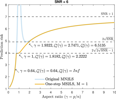
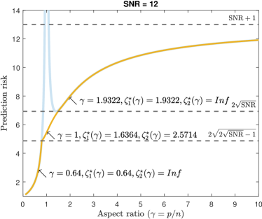
Figure S.5: Illustration of the optimal splitting of the aspect ratios for the one-step optimization with MN2LS base prediction procedure. Here, $(\zeta_{1}^{\star}(\gamma),\zeta_{2}^{\star}(\gamma))$ indicates the optimal splitting of the aspect ratio $\gamma$ for the first and second splits.

S.6.8 Lemmas on properties of risk profile of ridgeless regression

In this section, we collect helper lemmas used in the proof of Theorem S.6.16. All the lemmas in this section are quite elementary, and only abstracted out for ease of repeated use in the proof of Theorem S.6.16.

Lemma S.6.17 (Properties of ridgeless risk profile in the underparameterized regime).

The function $g:x\mapsto\frac{x}{1-x}$ over the domain $(0,1)$ has the following properties:

1. The function $g$ is increasing in $x$.

2. When $x\leq 0.5$, $g(x)\leq 1$.

3. When $x>0.5$, $g(x)>1$.

Proof.

The claims are easy to check. See Figure S.6 (the $x<1$ segment) for illustration. ∎

Lemma S.6.18 (Properties of ridgeless risk profile in the overparameterized regime).

Let $h(\cdot;s):x\mapsto s\left(1-\frac{1}{x}\right)+\frac{1}{x-1}$ be a function defined on the domain $x>1$, parametrized by $s\geq 0$. The function $h$ has the following properties:

1. When $s\leq 1$, the function is decreasing in $x$ and approaches the minimum value of $s$ as $x\to\infty$.

2. When $s>1$, the function attains the minimum value of $2\sqrt{s}-1$ at $x=\frac{\sqrt{s}}{\sqrt{s}-1}$.

3. When $s>1$, $h(x;s)>1$ for all $x>1$.

4. For $x>\frac{\sqrt{s}}{\sqrt{s}-1}$, the function is increasing in $x$.

5. The function $s\mapsto h(x;s)$ is increasing in $s$ for $s\geq 0$ for any fixed $x>1$.

Proof.

The first property is easy to check. The second property follows elementary calculus. The third property follows from the second property. The fourth property follows by inspecting the derivative of $h(\cdot;s)$ for $x>\frac{\sqrt{s}}{\sqrt{s}-1}$. The fifth property is easy to check. See Figure S.6 (the $x>1$ segment) for illustration.

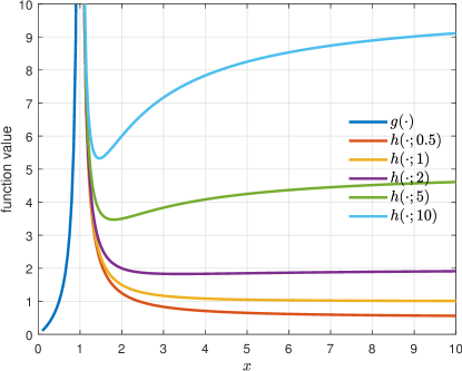
Figure S.6: Illustration of ridgeless risk profile with varying SNR.

∎

Lemma S.6.19 (Properties of ridgeless one-step ingredient risk profile in the overparameterized regime).

Let $h(x;s):x\mapsto s\left(1-\frac{1}{x}\right)+\frac{1}{x-1}$ be a function defined on the domain $x>1$, parameterized by $s\geq 1$. Let $g:(x,y)\mapsto h(y;h(x;s))$ be a function defined on the domain $x>1$ and $y>1$, parameterized by $s\geq 1$. The function $g$ has the following properties:

1. For any fixed $y>1$, the function $g$ is minimized at $x=\frac{\sqrt{s}}{\sqrt{s}-1}$ and increasing in $x$ for $x\geq\frac{\sqrt{s}}{\sqrt{s}-1}$.

2. For any fixed $x>1$, $g(x,y)$ is increasing over $y\geq\frac{\sqrt{h(x;s)}}{\sqrt{h(x;s)}-1}$.

Proof.

The first claim follows from Lemma S.6.18 (2), (4), (5). The second claim follows from Lemma S.6.18 (4). ∎

S.6.9 Control of additive error term in expectation

The following remark complements Remark 2.8 and specifies the growth allowed conditions on $\widehat{\sigma}_{\Xi}$ to ensure that $\mathbb{E}[\Delta_{n}^{\mathrm{add}}]=o(1)$.

Remark S.6.20 (Tolerable growth rates on $\widehat{\sigma}_{\Xi}$ for $\mathbb{E}\Delta_{n}^{\mathrm{add}}=o(1)$).

Suppose $|\Xi|\leq n^{S}$ for some $S<\infty$. Under the setting of Lemma 2.4, if for some $t\geq 1$,

$$\max_{\xi\in\Xi}\,\|\widehat{\sigma}_{\xi}\|_{L_{t}}=o\left(\frac{n_{\mathrm{te}}^{1/2}}{n^{-A+(A+S)/t}}\right),$$

then $\mathbb{E}[\Delta_{n}^{\mathrm{add}}]=o(1)$. On the other hand, under the setting of Lemma 2.5, if

$$\max_{\xi\in\Xi}\,\|\widehat{\sigma}_{\xi}\|_{L_{2}}=o\left(\frac{n_{\mathrm{te}}^{1/2}}{n^{(S-A)/2}}\right)$$

then $\mathbb{E}[\Delta_{n}^{\mathrm{add}}]=o(1)$. The remark follows simply by observing that the first term in the expectation bounds (11) and (13) for both Lemmas 2.4 and 2.5 are $o(1)$, while the second term in Lemma 2.4 is of order

$$O\left(\frac{n^{-A/r+S/t}}{n_{\mathrm{te}}^{1/2}}\right)\max_{\xi\in\Xi}\|\widehat{\sigma}_{\xi}\|_{L_{t}},$$

for $r,t\geq 1$ and $1/r+1/t=1$, and the second term in Lemma 2.5 is of order

$$O\left(\frac{n^{-A/2+S/2}}{n_{\mathrm{te}}^{1/2}}\right)\max_{\xi\in\Xi}\|\widehat{\sigma}_{\xi}\|_{L_{2}}.$$

It is worth mentioning that one can also derive suitable growth rates on $\widehat{\kappa}_{\Xi}$ that yield conditions for $\mathbb{E}[\Delta_{n}^{\mathrm{mul}}]=o(1)$. However, this does not directly lead to control of $\mathbb{E}[R({\widehat{f}}^{\mathrm{cv}}(\cdot;\mathcal{D}_{n}))]$ in the multiplicative form (8). This is because of the denominator $(1-\Delta_{n}^{\mathrm{mul}})_{+}$ appearing in (8). For every $n$, there is a non-zero probability that the denominator $(1-\Delta_{n}^{\mathrm{mul}})_{+}$ is zero. Hence, the right hand side of (8) may not have a finite expectation in general. However, assuming $\mathbb{E}[R({\widehat{f}}^{\xi}(\cdot;\mathcal{D}_{n}))]<C$ for some $C<\infty$ for all $\xi\in\Xi$, one can control $\mathbb{E}[R({\widehat{f}}^{\mathrm{cv}}(\cdot;\mathcal{D}_{n}))]$ by explicitly analyzing $\mathbb{P}(\Delta^{\mathrm{mul}}_{n}>1/2)$, and using the bound

$$R({\widehat{f}}^{\mathrm{cv}}(\cdot;\mathcal{D}_{n})) \leq\frac{1+\Delta_{n}^{\mathrm{mul}}}{(1-\Delta_{n}^{\mathrm{mul}})_{+}}\cdot\min_{\xi\in\Xi}R({\widehat{f}}^{\xi}(\cdot;\mathcal{D}_{\mathrm{tr}}).\mathbbm{1}_{\Delta_{n}^{\mathrm{mul}}\leq 1/2}+\sum_{\xi\in\Xi}R({\widehat{f}}^{\xi}(\cdot;\mathcal{D}_{n}))\mathbbm{1}_{\Delta_{n}^{\mathrm{mul}}>1/2}.$$

S.6.10 A lemma on norm equivalence implications

The following lemma formalizes various norm equivalence implications mentioned in Remarks 2.19 and 2.20.

Proposition S.6.21 (Norm equivalence implications).

The following statements hold.

1. Suppose a random $X$ satisfies $L_{4}-L_{2}$ equivalence, i.e., there exists a constant $C$ such that $\mathbb{E}[X^{4}]\leq C\mathbb{E}[X^{2}]$, then the random variable satisfies $L_{2}-L_{1}$ equivalence, i.e., there exists a constant $C$ such that $\mathbb{E}[X^{2}]\leq C\mathbb{E}[|X|]$.

2. A random variable $W$ satisfying $\psi_{2}-L_{2}$ equivalence also satisfies $\psi_{1}-L_{1}$ equivalence.

Proof.

We will use the fact that the map $p\mapsto\log\mathbb{E}[|X|^{p}]$ ($p\geq 1$) is convex. In other words, for $\lambda\in(0,1)$, we have

$$\log\mathbb{E}[|X|^{\lambda r+(1-\lambda)s}]\leq\lambda\log\mathbb{E}[|X|^{r}]+(1-\lambda)\log\mathbb{E}[|X|^{s}]$$ (E.135)

We now use $r=4$ and $s=1$, and $\lambda=1/3$ so that $\lambda r+(1-\lambda)s=2$. Plugging these choices in (E.135) yields

$$\log\mathbb{E}[X^{2}]\leq\frac{1}{3}\log\mathbb{E}[X^{4}]+\frac{2}{3}\log\mathbb{E}[|X|].$$

In terms of norms the inequality then becomes

$$2\log\|X\|_{L_{2}}\leq\frac{4}{3}\log\|X\|_{L_{4}}+\frac{2}{3}\log\|X\|_{L_{1}}.$$

This yields

$$\frac{2}{3}\log\frac{\|X\|_{L_{2}}}{\|X\|_{L_{1}}}\leq\frac{4}{3}\log\frac{\|X\|_{L_{4}}}{\|X\|_{L_{2}}}.$$

Manipulating both sides, we end up with

$$\frac{\|X\|_{L_{2}}}{\|X\|_{L_{1}}}\leq\left(\frac{\|X\|_{L_{4}}}{\|X\|_{L_{2}}}\right)^{2}$$

as desired.

The second facts follows because $\psi_{2}-L_{2}$ equivalence implies $L_{p}-L_{2}$ equivalence for each $p\geq 1$, i.e., for each $p\geq 1$, we have that

$$\|W\|_{L_{p}}\leq C\sqrt{p}\|W\|_{L_{2}},$$

for an universal constant $C$; see Vershynin, (2018, Proposition 2.5.2), for example. This in particular implies, $L_{4}-L_{2}$ equivalence, and by the first fact implies $L_{2}-L_{1}$. Thus, there exists a universal constant $C$ such that

$$\|W\|_{L_{2}}\leq\|W\|_{L_{1}}.$$

Combining with the inequality above, we then get for $p\geq 1$,

$$\|W\|_{L_{p}}\leq C\sqrt{p}\|W\|_{L_{1}}\leq Cp\|W\|_{L_{1}}.$$

Now, using Vershynin, (2018, Proposition 2.7.1), this implies $\psi_{1}-L_{1}$ equivalence.

Alternatively, assuming $\psi_{2}-L_{2}$ equivalence, observe the following chain of inequalities:

$$C\|X\|_{L_{4}}\overset{(a)}{\leq}\|X\|_{\psi_{1}}\overset{(b)}{\leq}(\log 2)^{1/2}\|X\|_{\psi_{2}}\overset{(c)}{\leq}C\|X\|_{L_{2}}$$

where $(a)$ follows from Vershynin, (2018, Proposition 2.5.2), $(b)$ follows from Wellner and van der Vaart, (2013, Problem 2.2.5), $(c)$ follows from the assumed $\psi_{2}-L_{2}$ equivalence. Finally, since $\psi_{2}-L_{2}$ equivalence implies $L_{4}-L_{2}$ equivalence, and from the fact this implies $L_{2}-L_{1}$ equivalence concludes the proof.

Figure S.7 visually summarizes the norm equivalence implications. ∎

Figure S.7: Visual illustration of norm equivalence implications discussed in Remarks 2.19 and 2.20, and in the proof of Proposition S.6.21. In the figure, $\framebox{A}\Rightarrow\framebox{B}$ indicates that equivalence $A$ implies equivalence $B$.

S.6.11 Proof of (63)

Below we prove the risk decomposition (63) for the ingredient zero-step predictor under squared error loss. The proof follows from the following iterated bias-variance decomposition.

$$\mathbb{E}\big{[}(Y_{0}-{\widetilde{f}}_{M}(X_{0};\mathcal{D}_{\mathrm{tr}}))^{2}\mathrel{|}\mathcal{D}_{\mathrm{tr}}\big{]}$$

$$=\mathbb{E}\Big{[}\mathbb{E}\big{[}(Y_{0}-{\widehat{f}}_{M}(X_{0};\mathcal{D}_{\mathrm{tr}}))^{2}\mathrel{|}\mathcal{D}_{\mathrm{tr}},(X_{0},Y_{0})\big{]}\mid\mathcal{D}_{\mathrm{tr}}\Big{]}$$

$$=\mathbb{E}\Big{[}\Big{(}Y_{0}-\mathbb{E}\big{[}{\widetilde{f}}_{M}(X_{0};\mathcal{D}_{\mathrm{tr}})\mathrel{|}\mathcal{D}_{\mathrm{tr}},(X_{0},Y_{0})\big{]}\Big{)}^{2}\mathrel{\big{|}}\mathcal{D}_{\mathrm{tr}}\Big{]}+\mathbb{E}\Big{[}\mathrm{Var}\big{(}{\widetilde{f}}_{M}(X_{0};\mathcal{D}_{\mathrm{tr}})\mathrel{|}\mathcal{D}_{\mathrm{tr}},(X_{0},Y_{0})\big{)}\mathrel{\big{|}}\mathcal{D}_{\mathrm{tr}}\Big{]}$$

$$=\mathbb{E}\left[\left(Y_{0}-\frac{1}{\binom{n}{k_{n}}}\sum_{i_{1},\dots,i_{k_{n}}}{\widetilde{f}}\big{(}X_{0};\{(X_{i_{j}},Y_{i_{j}}):1\leq j\leq k_{n}\}\big{)}\right)^{2}\mathrel{\Bigg{|}}\mathcal{D}_{\mathrm{tr}}\right]+\mathbb{E}\left[\frac{1}{M}\mathrm{Var}\left({\widetilde{f}}(X_{0};\mathcal{D}_{\mathrm{tr},1})\mathrel{\big{|}}\mathcal{D}_{\mathrm{tr}},(X_{0},Y_{0})\right)\mathrel{\bigg{|}}\mathcal{D}_{\mathrm{tr}}\right]$$

$$=R({\widetilde{f}}_{\infty}(\cdot;\mathcal{D}_{\mathrm{tr}}))+\frac{1}{M}\mathbb{E}\left[\frac{1}{\binom{n}{k_{n}}}\sum_{i_{1},\dots,i_{k_{n}}}\left({\widetilde{f}}\big{(}X_{0};\{(X_{0},Y_{0}):1\leq j\leq k_{n}\}\big{)}-{\widetilde{f}}_{\infty}(X_{0};\mathcal{D}_{\mathrm{tr}})\right)^{2}\mathrel{\bigg{|}}\mathcal{D}_{\mathrm{tr}}\right],$$

where in the last line $f_{\infty}(\cdot;\mathcal{D}_{\mathrm{tr}}):\mathbb{R}^{p}\to\mathbb{R}$ is defined such that for any $x\in\mathbb{R}^{p}$

$${\widetilde{f}}_{\infty}(x;\mathcal{D}_{\mathrm{tr}})=\frac{1}{\binom{n}{k_{n}}}\sum_{1\leq i_{1}<\ldots<i_{k_{n}}\leq n_{\mathrm{tr}}}{\widetilde{f}}(x;\{(X_{i_{j}},Y_{i_{j}}):1\leq j\leq k_{n}\}).$$

S.7 Calculus of deterministic equivalents

We use the language of deterministic equivalents in the proofs of Proposition 3.14 and Proposition 4.11 in Section S.3 and Section S.5, respectively. In this section, we provide a basic review of the definitions and useful calculus rules. For more details, see Dobriban and Sheng, (2021).

Definition S.7.1.

Consider sequences $\{A_{p}\}_{p\geq 1}$ and $\{B_{p}\}_{p\geq 1}$ of (random or deterministic) matrices of growing dimension. We say that $A_{p}$ and $B_{p}$ are equivalent and write $A_{p}\simeq B_{p}$ if $\lim_{p\to\infty}|\mathop{\mathrm{tr}}[C_{p}(A_{p}-B_{p})]|=0$ almost surely for any sequence $C_{p}$ matrices with bounded trace norm such that $\limsup\|C_{p}\|_{\mathrm{tr}}<\infty$ as $p\to\infty$.

An observant reader will notice that Dobriban and Sheng, (2021) use the notation $A_{p}\asymp B_{p}$ to denote deterministic asymptotic equivalence. In this paper, we instead prefer to use the notation $A_{p}\simeq B_{p}$ for such equivalence to stress the fact that this equivalence is exact in the limit rather than up to constants as the “standard” use of the asymptotic notation $\asymp$ would hint at.

Lemma S.7.2 (Calculus of deterministic equivalents, Dobriban and Wager, (2018), Dobriban and Sheng, (2021)).

Let $A_{p}$, $B_{p}$, and $C_{p}$ be sequences of (random or deterministic) matrices. The calculus of deterministic equivalents satisfy the following properties:

1. Equivalence: The relation $\simeq$ is an equivalence relation.

2. Sum: If $A_{p}\simeq B_{p}$ and $C_{p}\simeq D_{p}$, then $A_{p}+C_{p}\simeq B_{p}+D_{p}$.

3. Product: If $A_{p}$ a sequence of matrices with bounded operator norms, i.e., $\|A_{p}\|_{\mathop{op}}<\infty$, and $B_{p}\simeq C_{p}$, then $A_{p}B_{p}\simeq A_{p}C_{p}$.

4. Trace: If $A_{p}\simeq B_{p}$, then $\mathop{\mathrm{tr}}[A_{p}]/p-\mathop{\mathrm{tr}}[B_{p}]/p\to 0$ almost surely.

5. Differentiation: Suppose $f(z,A_{p})\simeq g(z,B_{p})$ where the entries of $f$ and $g$ are analytic functions in $z\in S$ and $S$ is an open connected subset of $\mathbb{C}$. Suppose for any sequence $C_{p}$ of deterministic matrices with bounded trace norm we have $|\mathop{\mathrm{tr}}[C_{p}(f(z,A_{p})-g(z,B_{p}))]|\leq M$ for every $p$ and $z\in S$. Then we have $D_{z}(f(z,A_{p}))\simeq D_{z}(g(z,B_{p}))$ for every $z\in S$, where the derivatives are taken entry-wise with respect to $z$.

We record deterministic equivalent for the standard ridge resolvent.

Lemma S.7.3 (Deterministic equivalent for basic ridge resolvent, adapted from Theorem 1 of Rubio and Mestre, (2011); see also Theorem 3.1 of Dobriban and Sheng, (2021)).

Suppose $X_{i}\in\mathbb{R}^{p}$, $1\leq i\leq n$, are i.i.d. random vectors where each $X_{i}=Z_{i}\Sigma^{1/2}$, where $Z_{i}$ contains i.i.d. entries $Z_{ij}$, $1\leq j\leq p$, with $\mathbb{E}[Z_{ij}]=0$, $\mathbb{E}[Z_{ij}^{2}]=1$, and $\mathbb{E}[|Z_{ij}|^{8+\alpha}]\leq M_{\alpha}$ for some $\alpha>0$ and $M_{\alpha}<\infty$, and $\Sigma\in\mathbb{R}^{p\times p}$ is a positive semidefinite matrix such that $0\preceq\Sigma\preceq r_{\max}I_{p}$ for some constant (independent of $p$) $r_{\max}<\infty$. Let $\bm{X}\in\mathbb{R}^{n\times p}$ the matrix with $X_{i}$, $1\leq i\leq n$ as rows and ${\widehat{\bm{\Sigma}}}\in\mathbb{R}^{p\times p}$ denote the random matrix $\bm{X}^{\top}\bm{X}/n$. Define $\gamma_{n}=p/n$. Then, for $z\in\mathbb{C}^{>0}$, as $n,p\to\infty$ such that $0<\liminf\gamma_{n}\leq\limsup\gamma_{n}<\infty$, we have

$$({\widehat{\bm{\Sigma}}}-zI_{p})^{-1}\simeq(c(e(z;\gamma_{n}))\Sigma-zI_{p})^{-1},$$ (E.136)

where $c(e(z;\gamma_{n}))$ is defined as

$$c(e(z;\gamma_{n}))=\frac{1}{1+\gamma_{n}e(z;\gamma_{n})},$$ (E.137)

and $e(z;\gamma_{n})$ is the unique solution in $\mathbb{C}^{>0}$ to the fixed-point equation

$$e(z;\gamma_{n})=\mathop{\mathrm{tr}}[\Sigma(c(e(z;\gamma_{n}))\Sigma-zI_{p})^{-1}]/p.$$ (E.138)

Furthermore, $e(z;\gamma_{n})$ is the Stieltjes transform of a certain positive measure on $\mathbb{R}_{\geq 0}$ with total mass $\mathop{\mathrm{tr}}[\Sigma]/p$.

We note that in defining $e(\lambda;\gamma_{n})$, it is also implicitly a parameterized by $\Sigma$. We suppress this dependence for notational simplicity, and only explicitly indicate dependence on $z$ and $\gamma_{n}$ that will be useful for our purposes.

Corollary S.7.4.

Assume the setting of Lemma S.7.3. For $\lambda>0$, we have

$$\lambda({\widehat{\bm{\Sigma}}}+\lambda I_{p})^{-1}\simeq(v(-\lambda;\gamma_{n})\Sigma+I_{p})^{-1},$$

where $v(-\lambda;\gamma_{n})$ is the unique solution to the fixed-point equation

$$\frac{1}{v(-\lambda;\gamma_{n})}=\lambda+\gamma_{n}\mathop{\mathrm{tr}}[\Sigma(v(-\lambda;\gamma_{n})\Sigma+I_{p})^{-1}]/p.$$

Proof.

From Lemma S.7.3, for $z\in\mathbb{C}^{>0}$, we have the basic equivalence for ridge resolvent

$$({\widehat{\bm{\Sigma}}}-zI_{p})^{-1}\simeq(c(e(z;\gamma_{n}))\Sigma-zI_{p})^{-1},$$ (E.139)

where $c(e(z;\gamma_{n}))$ is defined by (E.137) and and $e(z;\gamma_{n})$ is the unqiue solution in $\mathbb{C}^{>0}$ to the fixed-point equation (E.138). Substituting for $e(z;\gamma_{n})$ from (E.137) into (E.138), we can write the fixed-point equation for $c(e(z;\gamma_{n}))$ as

$$\frac{1}{c(e(z;\gamma_{n}))\gamma_{n}}-\frac{1}{\gamma_{n}}=\mathop{\mathrm{tr}}[\Sigma(c(e(z;\gamma_{n}))\Sigma-zI_{p})^{-1}]/p.$$ (E.140)

Manipulating (E.140), we can write

$$\frac{1}{c(e(z;\gamma_{n}))}-1=\gamma_{n}\mathop{\mathrm{tr}}[\Sigma(c(e(z;\gamma_{n}))\Sigma-zI_{p})^{-1}]/p=\frac{\gamma_{n}}{(-z)}\mathop{\mathrm{tr}}[\Sigma(c(e(z;\gamma_{n}))/(-z)\Sigma+I_{p})^{-1}]/p.$$ (E.141)

Moving $(-z)$ across in (E.141), we have equivalently the following equation for $c(e(z;\gamma_{n}))$:

$$\frac{(-z)}{c(e(z;\gamma_{n}))}+z=\gamma_{n}\mathop{\mathrm{tr}}[\Sigma(c(e(z;\gamma_{n}))/(-z))^{-1}]/p.$$ (E.142)

Now defining $c(e(z;\gamma_{n}))/(-z)$ by $v(z;\gamma_{n})$, the fixed-point equation (E.142) becomes

$$\frac{1}{v(z;\gamma_{n})}=-z+\gamma_{n}\mathop{\mathrm{tr}}[\Sigma(v(z;\gamma_{n})\Sigma+I_{p})^{-1}]/p.$$ (E.143)

Note that (E.143) is also known as the Silverstein equation (Silverstein,, 1995), and $v(z;\gamma_{n})$ as the companion Stieltjes transform. Along the same lines, from (E.139), we have

$$(-z)({\widehat{\bm{\Sigma}}}-zI_{p})^{-1}\simeq(-z)(c(e(z;\gamma_{n}))\Sigma-zI_{p})^{-1}=(c(e(z;\gamma_{n}))/(-z)\Sigma+I_{p})^{-1}.$$ (E.144)

Substituting for $v(z;\gamma_{n})$, we can thus write

$$(-z)({\widehat{\bm{\Sigma}}}-zI_{p})^{-1}\simeq(v(z;\gamma_{n})\Sigma+I_{p})^{-1}.$$ (E.145)

Now, taking $z=-\lambda$ in (E.143) and (E.145) yields the equivalence

$$\lambda({\widehat{\bm{\Sigma}}}+\lambda I_{p})^{-1}\simeq(v(-\lambda;\gamma_{n})\Sigma+I_{p})^{-1},$$

where $v(-\lambda;\gamma_{n})$ is the unique solution to the fixed point equation

$$\frac{1}{v(-\lambda;\gamma_{n})}=\lambda+\gamma_{n}\mathop{\mathrm{tr}}[\Sigma(v(-\lambda;\gamma_{n})\Sigma+I_{p})^{-1}]/p.$$

Finally, since $v(-\lambda;\gamma_{n})$ is a Stieltjes transform of a probability measure (with support on $\mathbb{R}_{\geq 0}$), we have that for $\operatorname{Re}(\lambda)>0$, by taking $\operatorname{Im}(\lambda)\to 0$, we have that $\operatorname{Im}(v(-\lambda;\gamma_{n}))\to 0$, and thus the statement follows. ∎

We remark that we will directly apply Corollary S.7.4 for a real $\lambda>0$ (in particular, in Lemma S.6.10). The limiting argument to go from a complex $\lambda$ to a real $\lambda$ follow as done in the proof of Corollary S.7.4. See, for example, proof of Theorem 5 in Hastie et al., (2019) (that uses Lemma 2.2 of Knowles and Yin, (2017)) for more details.

S.8 Useful concentration results

In this section, we gather statements of concentration results available in the literature that are used in the proofs in Sections S.1, S.3 and S.5.

Non-asymptotic statements

Tail bounds.

The following two tail bounds are used in the proofs of Lemmas 2.4, 2.5, 2.9 and 2.10 in Section S.1.

Lemma S.8.1 (Bernstein’s inequality, adapted from Theorem 2.8.1 of Vershynin, (2018)).

Let $Z_{1},\dots,Z_{n}$ be independent mean-zero sub-exponential random variables. Then, for every $t\geq 0$, we have

$$\mathbb{P}\left\{\left|\sum_{i=1}^{n}Z_{i}\right|\geq t\right\}\leq 2\exp\left(-c\min\left\{\frac{t^{2}}{\sum_{i=1}^{n}\|Z_{i}\|_{\psi_{1}}^{2}},\frac{t}{\max_{1\leq i\leq n}\|Z_{i}\|_{\psi_{1}}}\right\}\right),$$

where $c>0$ is an absolute constant. In other words, with probability at least $1-\eta$, we have

$$\left|\sum_{i=1}^{n}Z_{i}\right|\leq\max\left\{\sqrt{\frac{1}{c}\sum_{i=1}^{n}\|Z_{i}\|_{\psi_{1}}^{2}\log\left(\frac{2}{\eta}\right)},\frac{1}{c}\max_{1\leq i\leq n}\|Z_{i}\|_{\psi_{1}}\log\left(\frac{2}{\eta}\right)\right\}.$$

Lemma S.8.2 (Concentration for median-of-means (MOM) estimator, adapted from Theorem 2 of Lugosi and Mendelson, (2019)).

Let $W_{1},\dots,W_{n}$ be i.i.d. random variables with mean $\mu$ and variance bounded by $\sigma^{2}$. Suppose we split the data $\{W_{1},\dots,W_{n}\}$ into $B$ batches $\mathcal{T}_{1},\dots,\mathcal{T}_{B}$. Let $\widehat{\mu}_{b}$ be sample mean computed on $\mathcal{T}_{b}$ for $b=1,\dots,B$. Define

$$\widehat{\mu}_{B}^{\texttt{MOM}}:=\mathrm{median}(\widehat{\mu}_{1},\dots,\widehat{\mu}_{B}).$$

Then, we have

$$\mathbb{P}\left\{\left|\widehat{\mu}_{B}^{\texttt{MOM}}-\mu\right|>\sigma\sqrt{4B/n}\right\}\leq\exp(-B/8).$$

Thus, letting $0<\eta<1$ be a real number, $B=\lceil 8\log(1/\eta)\rceil$, with probability at least $1-\eta$,

$$\left|\widehat{\mu}_{B}^{\texttt{MOM}}-\mu\right|\leq\sigma\sqrt{\frac{32\log(1/\eta)}{n}}.$$

With $B=\lceil 8\log(1/\eta)\rceil$, we use the notation $\texttt{MOM}(\{W_{1},\ldots,W_{n}\},\eta)$ for $\widehat{\mu}_{B}^{\texttt{MOM}}$, that is,

$$\texttt{MOM}(\{W_{1},\ldots,W_{n}\},\eta)~{}:=~{}\widehat{\mu}^{\texttt{MOM}}_{\lceil 8\log(1/\eta)\rceil}.$$ (E.146)

Moment bounds.

The following two moment bounds imply Lemmas S.8.5 and S.8.6 that are used in the proofs of Proposition 3.14 and Corollary 4.9 in Section S.3 and Section S.5, respectively.

Lemma S.8.3 (Moment bound on centered linear form, adapted from Lemma 7.8 of Erdos and Yau, (2017)).

Let $\bm{Z}\in\mathbb{R}^{p}$ be a random vector containing i.i.d. entries $Z_{i}$, $i=1,\dots,n$, such that for each i, $\mathbb{E}[Z_{i}]=0$, $\mathbb{E}[Z_{i}^{2}]=1$, and $\mathbb{E}[|Z_{i}|^{k}]\leq M_{k}$. Let $a\in\mathbb{R}^{p}$ be a deterministic vector. Then,

$$\mathbb{E}[|a^{\top}\bm{Z}|^{q}]\leq C_{q}M_{q}\|a\|_{2}^{q}$$

for a constant $C_{q}$ that only depends on $q$.

Lemma S.8.4 (Moment bound on centered quadratic form, adapted from Lemma B.26 of Bai and Silverstein, (2010)).

Let $\bm{Z}\in\mathbb{R}^{n}$ be a random vector with i.i.d. entries $Z_{i}$, $i=1,\dots,n$, such that for each $i$, $\mathbb{E}[Z_{i}]=0$, $\mathbb{E}[Z_{i}^{2}]=1$, and $\mathbb{E}[|Z_{i}|^{k}]\leq M_{k}$ for $k>2$ and some constant $M_{k}$. Let $A\in\mathbb{R}^{p\times p}$ be a deterministic matrix. Then, for $q\geq 1$,

$$\mathbb{E}\big{[}|\bm{Z}^{\top}A\bm{Z}-\mathop{\mathrm{tr}}[A]|^{q}\big{]}\leq C_{q}\big{\{}(M_{4}\mathop{\mathrm{tr}}[AA^{\top}])^{q/2}+M_{2q}\mathop{\mathrm{tr}}[(AA^{\top})^{q/2}]\big{\}}$$

for a constant $C_{q}$ that only depends on $q$.

Asymptotic statements

As a consequence of Lemma S.8.3 and Lemma S.8.7, we have the following concentration of a linear form with independent components.

Lemma S.8.5 (Concentration of linear form with independent components).

Let $\bm{Z}\in\mathbb{R}^{p}$ be a random vector with i.i.d. entries $Z_{i}$, $i=1,\dots,p$ such that for each $i$, $\mathbb{E}[Z_{i}]=0$, $\mathbb{E}[|Z_{i}|^{4+\alpha}]\leq M_{\alpha}$ for some constant $M_{\alpha}<\infty$. Let $\bm{A}\in\mathbb{R}^{p}$ be a random vector independent of $\bm{Z}$ such that $\limsup_{p}\|\bm{A}_{p}\|^{2}/p\leq M_{n}$ almost surely for a constant $M_{n}<\infty$. Then, $\bm{A}^{\top}\bm{Z}/p\to 0$ almost surely as $p\to\infty$.

As a consequence of Lemma S.8.4 and Lemma S.8.7, we have the following concentration of a quadratic form with independent components.

Lemma S.8.6 (Concentration of quadratic form with independent components).

Let $\bm{Z}\in\mathbb{R}^{p}$ be a random vector with i.i.d. entries $Z_{i}$, $i=1,\dots,p$ such that for each i, $\mathbb{E}[Z_{i}]=0$, $\mathbb{E}[Z_{i}^{2}]=1$, $\mathbb{E}[|Z_{i}|^{4+\alpha}]\leq M_{\alpha}$ for some $\alpha>0$ and constant $M_{\alpha}<\infty$. Let $\bm{D}\in\mathbb{R}^{p\times p}$ be a random matrix such that $\limsup\|\bm{D}\|_{\textrm{op}}\leq M_{o}$ almost surely as $p\to\infty$ for some constant $M_{o}<\infty$. Then, $\bm{Z}^{\top}\bm{D}\bm{Z}/p-\mathop{\mathrm{tr}}[\bm{D}]/p\to 0$ almost surely as $p\to\infty$.

Lemma S.8.7 (Moment version of the Borel-Cantelli lemma).

Let $\{Z_{n}\}_{n\geq 1}$ be a sequence of real-valued random variables such that the sequence $\{\mathbb{E}|Z_{n}|^{q}\}_{n\geq 1}$ is summable for some $q>0$. Then, $Z_{n}\to 0$ almost surely as $n\to\infty$.

S.9 Notation

Below we list general notation used in this paper. Table 1 at the end of the manuscript provides a comprehensive list of some of the specific notation used throughout.

• We denote scalar random variables in regular upper case (e.g., $X$), and vector and matrix random variables in bold upper case (e.g., $\bm{X}$). We use calligraphic letters to denote sets (e.g., $\mathcal{D}$), and blackboard letters to denote some specials sets listed next.

• We use $\mathbb{N}$ to denote the set of natural numbers. We use $\mathbb{Q}$ to denote the set of rational numbers, $\mathbb{Q}_{>0}$ to denote the set of positive rational numbers; $\mathbb{R}$ to denote the set of real numbers, $\mathbb{R}_{\geq 0}$ to denote the set of non-negative real numbers, $\mathbb{R}_{>0}$ to denote the set of positive real numbers; $\mathbb{C}$ to denote the set of complex numbers, $\mathbb{C}^{>0}$ to denote the upper half of the complex plane, i.e., $\mathbb{C}^{>0}=\{z\in\mathbb{C}:\operatorname{Im}(z)>0\}$.

• For a real number $a$, $(a)_{+}$ denotes its positive part, $\lfloor a\rfloor$ denotes its floor, $\lceil a\rceil$ denotes its ceiling, $\operatorname{sgn}(a)$ denotes its sign. For a complex number $z$, $\operatorname{Re}(z)$ denotes its real part, $\operatorname{Im}(z)$ denotes its imaginary part, $\overline{z}$ denote its conjugate, $|z|$ denotes its absolute value.

• For a set $\mathcal{A}$, $|\mathcal{A}|$ denotes its cardinality, $\mathcal{A}^{\complement}$ denotes its complement, $\mathbbm{1}_{\mathcal{A}}$ denotes its indicator function. For a function $f$, $\partial/\partial x[f]$ denotes its partial derivative with respect to variable $x$. We also use $f^{\prime}$ to denote derivative of $f$ when it is clear from the context.

• For an event $A$, $\mathbb{P}(A)$ denotes its probability, and $\mathbbm{1}_{A}$ its indicator random variable. For a random variable $X$, $\mathbb{E}[X]$ denotes its expectation, $\mathop{\mathrm{Var}}(X)=\mathbb{E}[(X-\mathbb{E}[X])^{2}]$ denotes its variance; $\mathbb{E}[X^{r}]$ denotes its $r$-th moment, $\mathbb{E}[|X|^{r}]$ denotes its $r$-th absolute moment, $\|X\|_{L_{r}}=(\mathbb{E}[|X|^{r}])^{1/r}$ denotes its $L_{r}$ norm, for a real number $r\geq 1$; $\|X\|_{\psi}$ denotes its $\psi$ norm for an Orlicz function $\psi$; see Section 2.2 for more details.

• For a vector $a\in\mathbb{R}^{p}$, $\|a\|_{r}$ denotes its $\ell_{r}$ norm for $r\geq 1$, $\|a\|_{A}=\sqrt{a^{\top}Aa}$ denotes its norm with respect to a positive semidefinite matrix $A\in\mathbb{R}^{p\times p}$.

• For a matrix $A\in\mathbb{R}^{n\times p}$, $A^{\top}\in\mathbb{R}^{p\times n}$ denote its transpose, $A^{\dagger}\in\mathbb{R}^{p\times n}$ denotes the its Moore-Penrose inverse, $\|A\|_{\mathop{op}}$ denotes its operator norm, $\|A\|_{\mathop{\mathrm{tr}}}$ denotes its trace norm or nuclear norm ($\|A\|_{\mathop{\mathrm{tr}}}=\mathop{\mathrm{tr}}[(A^{\top}A)^{1/2}]=\sum_{i}\sigma_{i}(A))$, where $\sigma_{1}(A)\geq\sigma_{2}(A)\geq\dots$ denote its singular values in non-increasing order. For a square matrix $A\in\mathbb{R}^{p\times p}$, $\mathop{\mathrm{tr}}[A]=\sum_{i=1}^{p}A_{ii}$ denotes its trace. A $p$-dimensional identity matrix is denoted as $I_{p}$ or simply $I$ when it is clear from the context.

• For a $p\times p$ positive semidefinite matrix $A$ with eigenvalue decomposition $A=VRV^{\top}$ for an orthonormal matrix $V$ and a diagonal matrix $R$, and a function $f:\mathbb{R}_{\geq 0}\to\mathbb{R}_{\geq 0}$, we denote by $f(A)$ the $p\times p$ positive semidefinite matrix $Vf(R)V^{\top}$, where $f(R)$ is a $p\times p$ diagonal matrix obtained by applying the function $f$ to each diagonal entry of $R$.

• For two sequences of matrices $A_{n}$ and $B_{n}$, we use the notation $A_{n}\simeq B_{n}$ to denote a certain notion of asymptotic equivalence; see Section S.7 for more details. For symmetric matrices $A$ and $B$, $A\preceq B$ denotes the Loewner ordering to mean that the matrix $B-A$ is positive semidefinite.

• We write $a\asymp b$ when there exist absolute constants $C_{l}$ and $C_{u}$ such that $C_{l}\leq a/b\leq C_{u}$. We write $a\lesssim b$ when there exists an absolute constant $C$ such that $a\leq Cb$.

• We use $O$ and $o$ to denote the big-$O$ and little-$o$ asymptotic notation, respectively. We use $O_{p}$ and $o_{p}$ to denote the probabilistic big-$O$ and little-$o$ asymptotic notation, respectively. We denote convergence in probability by $\xrightarrow{\text{p}}$, almost sure convergence by $\xrightarrow{\text{a.s.}}$, weak convergence by $\xrightarrow{\text{d}}$.

• Finally, we use generic letters $C,C_{1},C_{2},\dots$ to denote constants whose value may change from line to line.

Notation	Meaning (Location in the paper)
$(X,Y)$	feature vector $X\in\mathbb{R}^{p}$ and response variable $Y\in\mathbb{R}$ (Section 2.1)
$\mathcal{D}_{n}=\{(X_{i},Y_{i})\}_{i=1}^{n}$	dataset with $n$ observations $(X_{i},Y_{i})$, $1\leq i\leq n$ (Section 2.1)
${\widehat{f}}(\cdot;\mathcal{D}_{n}):\mathbb{R}^{p}\to\mathbb{R}$	predictor fitted on dataset $\mathcal{D}_{n}$ using prediction procedure ${\widehat{f}}$ (Section 2.1)
$\ell:\mathbb{R}\times\mathbb{R}\to\mathbb{R}_{\geq 0}$	non-negative loss function (Section 2.1)
$\ell(Y_{0},{\widehat{f}}(X_{0};\mathcal{D}_{n}))$	prediction loss of predictor ${\widehat{f}}(\cdot;\mathcal{D}_{n})$ evaluated at test point $(X_{0},Y_{0})$ (Section 2.1)
$R({\widehat{f}}(\cdot;\mathcal{D}_{n}))$	prediction risk of predictor ${\widehat{f}}(\cdot;\mathcal{D}_{n})$ (5)
${\widehat{R}}({\widehat{f}}(\cdot;\mathcal{D}_{n}))$	estimator of prediction risk of ${\widehat{f}}(\cdot;\mathcal{D}_{n})$ (Section 2.1)
${\widehat{f}}^{\mathrm{cv}}(\cdot;\mathcal{D}_{n})$	cross-validated predictor fitted using dataset $\mathcal{D}_{n}$ (Algorithm 1)
${\widehat{f}}^{\xi}$, $\xi\in\Xi$	collection of prediction procedures indexed by set $\Xi$ (Algorithm 1)
$n_{\mathrm{tr}}$, $n_{\mathrm{te}}$	number of train and test observations (Algorithm 1)
$\mathcal{D}_{\mathrm{tr}},\mathcal{D}_{\mathrm{te}}$	random split of $\mathcal{D}_{n}$ into train and test datasets with $n_{\mathrm{tr}}$ and $n_{\mathrm{te}}$ observations (Algorithm 1)
$\mathcal{I}_{\mathrm{tr}},\mathcal{I}_{\mathrm{te}}$	disjoint subsets of $\mathcal{I}_{n}:=\{1,\dots,n\}$ that are index sets for $\mathcal{D}_{\mathrm{tr}}$ and $\mathcal{D}_{\mathrm{te}}$ (Algorithm 1)
CEN, AVG, MOM	centering procedure, averaging, median-of-means (2, 3)
$\eta$	parameter in median-of-means (E.146)
$\Delta_{n}^{\mathrm{add}}$, $\Delta_{n}^{\mathrm{mul}}$	error terms in the additive and multiplicative oracle risk inequalities (6a, 6b)
$\widehat{\sigma}_{\xi}$, $\widehat{\sigma}_{\Xi}$	conditional second moment of loss and their max over $\Xi$ (Lemmas 2.4 and 2.5)
$\widehat{\kappa}_{\xi}$, $\widehat{\kappa}_{\Xi}$	conditional kurtosis-like parameter of loss and their max over $\Xi$ (Lemmas 2.9 and 2.10)
$\|\ell(Y_{0},{\widehat{f}}(X_{0};\mathcal{D}_{n}))\|_{\psi_{1}\mid\mathcal{D}_{n}}$	conditional $\psi_{1}$ norm of prediction loss (9)
$\|\ell(Y_{0},{\widehat{f}}(X_{0};\mathcal{D}_{n}))\|_{L_{r}\mid\mathcal{D}_{n}}$	conditional $L_{r}$ norm of prediction loss ($r\geq 1)$ (10)
${\widetilde{\beta}}_{\mathrm{ridge}}$, ${\widetilde{\beta}}_{\mathrm{lasso}}$, ${\widetilde{\beta}}_{\mathrm{mn2}}$, ${\widetilde{\beta}}_{\mathrm{mn1}}$	ridge, lasso, min $\ell_{2}$, $\ell_{1}$-norm least squares estimation procedures (20–24)
${\widetilde{f}}_{\mathrm{mn2}}$, ${\widetilde{f}}_{\mathrm{mn1}}$	min $\ell_{2}$, $\ell_{1}$-norm least squares prediction procedures (22, 25)
${\widehat{f}}^{\mathrm{zs}}(\cdot;\mathcal{D}_{n})$	zero-step predictor fitted on dataset $\mathcal{D}_{n}$ (Algorithm 2)
$\nu\in(0,1)$	exponent for block sizes $\lfloor n^{\nu}\rfloor$ in zero-step prediction procedure (Algorithm 2)
$n_{\xi}$	$n-\xi\lfloor n^{\nu}\rfloor$ (Algorithm 2)
$M$	number of sub-samples for averaging for zero-step ingredient predictor (26)
$\mathcal{D}_{\mathrm{tr}}^{\xi,j}$, $1\leq j\leq M$	random subset of $\mathcal{D}_{\mathrm{tr}}$ of size $n_{\xi}$ (Algorithm 2)
${\widetilde{f}}(\cdot;\mathcal{D}_{\mathrm{tr}}^{\xi,j})$	zero-step ingredient predictor fitted on dataset $\mathcal{D}_{\mathrm{tr}}^{\xi,j}$ using base prediction procedure ${\widetilde{f}}$ (26)
$R^{\mathrm{det}}(m;{\widetilde{f}})$	deterministic approximation to $R({\widetilde{f}}(\cdot;\mathcal{D}_{m}))$ (Definition 3.2)
$R^{\mathrm{det}}_{\nearrow}(n;{\widetilde{f}})$	monotonized deterministic approximation at sample size $n$ under general asymptotics (30)
PA($\gamma$)	proportional asymptotics regime (PA($\gamma$))
DETPA-0	assumption of deterministic risk approximation to conditional risk under PA (DETPA-0)
DETPAR-0	reduction of assumption DETPA-0 (Lemma 3.8, DETPAR-0)
$R^{\mathrm{det}}(p_{m}/m;{\widetilde{f}})$	deterministic risk approximation at aspect ratio $p_{m}/m$ under PA (Section 3.3.1)
$\xi_{n}^{\star}$	optimal sequence of $\xi$ for zero-step monotonized risk approximation (30, DETPA-0)
PRG-0-C1,C2	deterministic risk approximation program for zero-step (PRG-0-C1)–(PRG-0-C2)
$k_{m},p_{m}$	sample size and feature size when verifying zero-step profile assumption (Lemma 3.8)
$\rho^{2}$, $\sigma^{2}$, $\mathrm{SNR}$	signal energy, noise energy, signal-to-noise ratio ($\rho^{2}$/$\sigma^{2}$) (Section 3.4)
$R_{\mathrm{mn2}}^{\mathrm{det}}(\phi;\rho^{2},\sigma^{2})$	MN2LS risk approximation at aspect ratio $\phi$, signal energy $\rho^{2}$, noise energy $\sigma^{2}$ (60)
${\widetilde{f}}_{\infty}(\cdot;\mathcal{D}_{\mathrm{tr}})$	zero-step ingredient predictor fitted on $\mathcal{D}_{n}$ with $M=\infty$ (62)
${\widehat{f}}^{\mathrm{os}}(\cdot;\mathcal{D}_{n})$	one-step predictor fitted on dataset $\mathcal{D}_{n}$ (Algorithm 3)
$(n_{1,\xi_{1}},n_{2,\xi_{2}})$	$(n-\xi_{1}\lfloor n^{\nu}\rfloor,\xi_{2}\lfloor n^{\nu}\rfloor)$ (Algorithm 3)
$(\mathcal{D}_{\mathrm{tr}}^{\xi_{1},j},\mathcal{D}_{\mathrm{tr}}^{\xi_{2},j})$, $1\leq j\leq M$	random pairs of disjoint subsets of $\mathcal{D}_{\mathrm{tr}}$ of sizes $(n_{1,\xi_{1}},n_{2,\xi_{2}})$ (Algorithm 3)
${\widetilde{f}}(\cdot;\mathcal{D}_{\mathrm{tr}}^{\xi_{1},j},\mathcal{D}_{\mathrm{tr}}^{\xi_{2},j})$	one-step ingredient predictor fitted on datasets $(\mathcal{D}_{\mathrm{tr}}^{\xi_{1},j},\mathcal{D}_{\mathrm{tr}}^{\xi_{2},j})$ (43)
DETPA-1, DETPA-1*	assumption of deterministic risk approximation to conditional risk under PA (DETPA-1)
DETPAR-1	reduction of assumption DETPA-1 (Lemma 4.1, DETPAR-1)
$R^{\mathrm{det}}(p/n_{1},p/n_{2};{\widetilde{f}})$	risk approximation of ingredient one-step predictor at aspect ratios $(p/n_{1},p/n_{2})$ (Section 4.3.1)
$(\xi_{1,n}^{\star},\xi_{2,n}^{\star})$	optimal pair of sequence of $\xi$ for one-step monotonized risk approximation (45)
PRG-1-C1,C2,C3	deterministic risk approximation program for one-step (PRG-1-C1)–(PRG-1-C3)
$k_{1,m},k_{2,m},p_{m}$	sample size and feature sizes when verifying one-step profile assumption (Lemma 4.1)
$w_{i}$, $r_{i}$, $1\leq i\leq p_{m}$	eigenvectors and eigenvalues of feature covariance matrix $\Sigma\in\mathbb{R}^{p_{m}\times p_{m}}$ (Section 4.3.2)
$\widehat{Q}_{n}$, $Q$	a certain random distribution and its weak limit (E.69)
$H_{p_{m}}$, $H$	empirical distribution of eigenvalues of $\Sigma$ and limiting spectral distribution (53)
$v(0;\phi_{2}),\widetilde{v}(0;\phi_{2}),\widetilde{v}_{g}(0;\phi_{2}),\Upsilon_{b}(\phi_{1},\phi_{2})$	scalars in risk approximation of one-step procedure with linear base procedure (55–58)
$R^{\mathrm{det}}_{\mathrm{mn2}}(\phi_{1},\phi_{2};\rho^{2},\sigma^{2})$	MN2LS one-step risk approx at aspect ratios $(\phi_{1},\phi_{2})$, signal energy $\rho^{2}$, noise energy $\sigma^{2}$ (60)

Table 1: Summary of some of the main notation used in the paper.

References

- Adamczak et al., (2010) Adamczak, R., Litvak, A., Pajor, A., and Tomczak-Jaegermann, N. (2010). Quantitative estimates of the convergence of the empirical covariance matrix in log-concave ensembles. Journal of the American Mathematical Society, 23(2):535–561.
- Adlam and Pennington, (2020) Adlam, B. and Pennington, J. (2020). The neural tangent kernel in high dimensions: Triple descent and a multi-scale theory of generalization. In International Conference on Machine Learning, pages 74–84. PMLR.
- Arlot and Celisse, (2010) Arlot, S. and Celisse, A. (2010). A survey of cross-validation procedures for model selection. Statistics surveys, 4:40–79.
- Austern and Zhou, (2020) Austern, M. and Zhou, W. (2020). Asymptotics of cross-validation. arXiv preprint arXiv:2001.11111.
- Bai and Silverstein, (2010) Bai, Z. and Silverstein, J. W. (2010). Spectral Analysis of Large Dimensional Random Matrices. Springer Series in Statistics. Second edition.
- Bartlett et al., (2020) Bartlett, P. L., Long, P. M., Lugosi, G., and Tsigler, A. (2020). Benign overfitting in linear regression. Proceedings of the National Academy of Sciences, 117(48):30063–30070.
- Bartlett et al., (2021) Bartlett, P. L., Montanari, A., and Rakhlin, A. (2021). Deep learning: a statistical viewpoint. arXiv preprint arXiv:2103.09177.
- Bayati et al., (2015) Bayati, M., Lelarge, M., and Montanari, A. (2015). Universality in polytope phase transitions and message passing algorithms. The Annals of Applied Probability, 25(2):753–822.
- Bayati and Montanari, (2011) Bayati, M. and Montanari, A. (2011). The dynamics of message passing on dense graphs, with applications to compressed sensing. IEEE Transactions on Information Theory, 57(2):764–785.
- Beirami et al., (2017) Beirami, A., Razaviyayn, M., Shahrampour, S., and Tarokh, V. (2017). On optimal generalizability in parametric learning. Advances in Neural Information Processing Systems, 30.
- (11) Belkin, M., Hsu, D., Ma, S., and Mandal, S. (2019a). Reconciling modern machine-learning practice and the classical bias–variance trade-off. Proceedings of the National Academy of Sciences, 116(32):15849–15854.
- Belkin et al., (2020) Belkin, M., Hsu, D., and Xu, J. (2020). Two models of double descent for weak features. SIAM Journal on Mathematics of Data Science, 2(4):1167–1180.
- (13) Belkin, M., Hsu, D. J., and Mitra, P. (2018a). Overfitting or perfect fitting? risk bounds for classification and regression rules that interpolate. Advances in neural information processing systems, 31.
- (14) Belkin, M., Ma, S., and Mandal, S. (2018b). To understand deep learning we need to understand kernel learning. In International Conference on Machine Learning, pages 541–549. PMLR.
- (15) Belkin, M., Rakhlin, A., and Tsybakov, A. B. (2019b). Does data interpolation contradict statistical optimality? In International Conference on Artificial Intelligence and Statistics, pages 1611–1619. PMLR.
- Bhatia, (1997) Bhatia, R. (1997). Matrix Analysis. Springer Graduate Texts in Mathematics.
- Bloemendal et al., (2016) Bloemendal, A., Knowles, A., Yau, H.-T., and Yin, J. (2016). On the principal components of sample covariance matrices. Probability theory and related fields, 164(1):459–552.
- Candes and Tao, (2006) Candes, E. J. and Tao, T. (2006). Near-optimal signal recovery from random projections: Universal encoding strategies? IEEE transactions on Information Theory, 52(12):5406–5425.
- Catoni, (2012) Catoni, O. (2012). Challenging the empirical mean and empirical variance: a deviation study. In Annales de l’IHP Probabilités et statistiques, volume 48, pages 1148–1185.
- Celentano et al., (2020) Celentano, M., Montanari, A., and Wei, Y. (2020). The lasso with general Gaussian designs with applications to hypothesis testing. arXiv preprint arXiv:2007.13716.
- Chen et al., (2020) Chen, L., Min, Y., Belkin, M., and Karbasi, A. (2020). Multiple descent: Design your own generalization curve. arXiv preprint arXiv:2008.01036.
- Chen and Lam, (2021) Chen, W.-K. and Lam, W.-K. (2021). Universality of approximate message passing algorithms. Electronic Journal of Probability, 26:1–44.
- Dar et al., (2021) Dar, Y., Muthukumar, V., and Baraniuk, R. G. (2021). A farewell to the bias-variance tradeoff? An overview of the theory of overparameterized machine learning. arXiv preprint arXiv:2109.02355.
- Derezinski et al., (2020) Derezinski, M., Liang, F. T., and Mahoney, M. W. (2020). Exact expressions for double descent and implicit regularization via surrogate random design. Advances in neural information processing systems, 33:5152–5164.
- Dobriban and Sheng, (2020) Dobriban, E. and Sheng, Y. (2020). Wonder: Weighted one-shot distributed ridge regression in high dimensions. J. Mach. Learn. Res., 21(66):1–52.
- Dobriban and Sheng, (2021) Dobriban, E. and Sheng, Y. (2021). Distributed linear regression by averaging. The Annals of Statistics, 49(2):918–943.
- Dobriban and Wager, (2018) Dobriban, E. and Wager, S. (2018). High-dimensional asymptotics of prediction: Ridge regression and classification. The Annals of Statistics, 46(1):247–279.
- Donoho and Montanari, (2016) Donoho, D. and Montanari, A. (2016). High dimensional robust -estimation: Asymptotic variance via approximate message passing. Probability Theory and Related Fields, 166(3):935–969.
- Donoho, (2006) Donoho, D. L. (2006). Compressed sensing. IEEE Transactions on Information Theory, 52(4):1289–1306.
- Donoho et al., (2009) Donoho, D. L., Maleki, A., and Montanari, A. (2009). Message-passing algorithms for compressed sensing. Proceedings of the National Academy of Sciences, 106(45):18914–18919.
- Duin, (1995) Duin, R. P. (1995). Small sample size generalization. In Proceedings of the Scandinavian Conference on Image Analysis, volume 2, pages 957–964.
- Erdos and Yau, (2017) Erdos, L. and Yau, H.-T. (2017). A Dynamical Approach to Random Matrix Theory. Courant Lecture Notes in Mathematics.
- Fan et al., (2017) Fan, J., Li, Q., and Wang, Y. (2017). Estimation of high dimensional mean regression in the absence of symmetry and light tail assumptions. Journal of the Royal Statistical Society: Series B (Statistical Methodology), 79(1):247–265.
- Frei et al., (2022) Frei, S., Chatterji, N. S., and Bartlett, P. L. (2022). Benign overfitting without linearity: Neural network classifiers trained by gradient descent for noisy linear data. arXiv preprint arXiv:2202.05928.
- Geiger et al., (2019) Geiger, M., Spigler, S., d’Ascoli, S., Sagun, L., Baity-Jesi, M., Biroli, G., and Wyart, M. (2019). Jamming transition as a paradigm to understand the loss landscape of deep neural networks. Physical Review E, 100(1):012115.
- Giordano et al., (2019) Giordano, R., Stephenson, W., Liu, R., Jordan, M., and Broderick, T. (2019). A swiss army infinitesimal jackknife. In International Conference on Artificial Intelligence and Statistics, pages 1139–1147. PMLR.
- Gribkova, (2020) Gribkova, N. V. (2020). Bounds for absolute moments of order statistics. In Exploring Stochastic Laws, pages 129–134. De Gruyter.
- Györfi et al., (2002) Györfi, L., Kohler, M., Krzyzak, A., and Walk, H. (2002). A Distribution-Free Theory of Nonparametric Regression. Springer Series in Statistics.
- Hastie et al., (2019) Hastie, T., Montanari, A., Rosset, S., and Tibshirani, R. J. (2019). Surprises in high-dimensional ridgeless least squares interpolation. arXiv preprint arXiv:1903.08560.
- Hastie et al., (2009) Hastie, T., Tibshirani, R., and Friedman, J. H. (2009). The Elements of Statistical Learning: Data Mining, Inference, and Prediction. Springer Series in Statistics.
- Hiriart-Urruty and Martınez-Legaz, (2003) Hiriart-Urruty, J.-B. and Martınez-Legaz, J.-E. (2003). New formulas for the Legendre–Fenchel transform. Journal of mathematical analysis and applications, 288(2):544–555.
- Hu and Lu, (2020) Hu, H. and Lu, Y. M. (2020). Universality laws for high-dimensional learning with random features. arXiv preprint arXiv:2009.07669.
- Karoui, (2013) Karoui, N. E. (2013). Asymptotic behavior of unregularized and ridge-regularized high-dimensional robust regression estimators: rigorous results. arXiv preprint arXiv:1311.2445.
- Karoui, (2018) Karoui, N. E. (2018). On the impact of predictor geometry on the performance on high-dimensional ridge-regularized generalized robust regression estimators. Probability Theory and Related Fields, 170(1):95–175.
- Karoui and Kösters, (2011) Karoui, N. E. and Kösters, H. (2011). Geometric sensitivity of random matrix results: consequences for shrinkage estimators of covariance and related statistical methods. arXiv preprint arXiv:1105.1404.
- Kini and Thrampoulidis, (2020) Kini, G. R. and Thrampoulidis, C. (2020). Analytic study of double descent in binary classification: The impact of loss. In 2020 IEEE International Symposium on Information Theory (ISIT), pages 2527–2532. IEEE.
- Knowles and Yin, (2017) Knowles, A. and Yin, J. (2017). Anisotropic local laws for random matrices. Probability Theory and Related Fields, 169(1):257–352.
- Latała, (1999) Latała, R. (1999). On the equivalence between geometric and arithmetic means for log-concave measures. Convex geometric analysis, 34:123–127.
- Lecué and Mendelson, (2012) Lecué, G. and Mendelson, S. (2012). General nonexact oracle inequalities for classes with a subexponential envelope. The Annals of Statistics, 40(2):832–860.
- LeCun et al., (1990) LeCun, Y., Kanter, I., and Solla, S. (1990). Second order properties of error surfaces: Learning time and generalization. Advances in neural information processing systems.
- Ledoit and Péché, (2011) Ledoit, O. and Péché, S. (2011). Eigenvectors of some large sample covariance matrix ensembles. Probability Theory and Related Fields, 151(1):233–264.
- Ledoux, (2001) Ledoux, M. (2001). The Concentration of Measure Phenomenon. American Mathematical Society.
- Li and Wei, (2021) Li, Y. and Wei, Y. (2021). Minimum -norm interpolators: Precise asymptotics and multiple descent. arXiv preprint arXiv:2110.09502.
- Liang and Rakhlin, (2020) Liang, T. and Rakhlin, A. (2020). Just interpolate: Kernel “ridgeless” regression can generalize. The Annals of Statistics, 48(3):1329–1347.
- Liang and Sur, (2020) Liang, T. and Sur, P. (2020). A precise high-dimensional asymptotic theory for boosting and minimum-l1-norm interpolated classifiers. arXiv preprint arXiv:2002.01586.
- Liu and Dobriban, (2019) Liu, S. and Dobriban, E. (2019). Ridge regression: Structure, cross-validation, and sketching. arXiv preprint arXiv:1910.02373.
- Loeve, (2017) Loeve, M. (2017). Probability Theory. Courier Dover Publications.
- Loog et al., (2020) Loog, M., Viering, T., Mey, A., Krijthe, J. H., and Tax, D. M. (2020). A brief prehistory of double descent. Proceedings of the National Academy of Sciences, 117(20):10625–10626.
- Lugosi and Mendelson, (2019) Lugosi, G. and Mendelson, S. (2019). Mean estimation and regression under heavy-tailed distributions: A survey. Foundations of Computational Mathematics, 19(5):1145–1190.
- Mei and Montanari, (2019) Mei, S. and Montanari, A. (2019). The generalization error of random features regression: Precise asymptotics and the double descent curve. Communications on Pure and Applied Mathematics.
- Mendelson and Zhivotovskiy, (2020) Mendelson, S. and Zhivotovskiy, N. (2020). Robust covariance estimation under norm equivalence. The Annals of Statistics, 48(3):1648–1664.
- Mhammedi, (2021) Mhammedi, Z. (2021). Risk monotonicity in statistical learning. Advances in Neural Information Processing Systems.
- Minsker, (2015) Minsker, S. (2015). Geometric median and robust estimation in banach spaces. Bernoulli, 21(4):2308–2335.
- Minsker, (2018) Minsker, S. (2018). Sub-gaussian estimators of the mean of a random matrix with heavy-tailed entries. The Annals of Statistics, 46(6A):2871–2903.
- Minsker and Wei, (2020) Minsker, S. and Wei, X. (2020). Robust modifications of U-statistics and applications to covariance estimation problems. Bernoulli, 26(1):694–727.
- Miolane and Montanari, (2021) Miolane, L. and Montanari, A. (2021). The distribution of the lasso: Uniform control over sparse balls and adaptive parameter tuning. The Annals of Statistics, 49(4):2313–2335.
- Mitra, (2019) Mitra, P. P. (2019). Understanding overfitting peaks in generalization error: Analytical risk curves for and penalized interpolation. arXiv preprint arXiv:1906.03667.
- Montanari and Nguyen, (2017) Montanari, A. and Nguyen, P.-M. (2017). Universality of the elastic net error. In 2017 IEEE International Symposium on Information Theory (ISIT), pages 2338–2342. IEEE.
- Montanari et al., (2019) Montanari, A., Ruan, F., Sohn, Y., and Yan, J. (2019). The generalization error of max-margin linear classifiers: High-dimensional asymptotics in the overparametrized regime. arXiv preprint arXiv:1911.01544.
- Mücke et al., (2021) Mücke, N., Reiss, E., Rungenhagen, J., and Kleinb, M. (2021). Data splitting improves statistical performance in overparameterized regimes. arXiv preprint arXiv:2110.10956.
- Munkres, (2000) Munkres, J. R. (2000). Topology. Pearson Prentice Hall. Second Edition.
- Muthukumar et al., (2020) Muthukumar, V., Vodrahalli, K., Subramanian, V., and Sahai, A. (2020). Harmless interpolation of noisy data in regression. IEEE Journal on Selected Areas in Information Theory, 1(1):67–83.
- Nakkiran, (2019) Nakkiran, P. (2019). More data can hurt for linear regression: Sample-wise double descent. arXiv preprint arXiv:1912.07242.
- Nakkiran et al., (2019) Nakkiran, P., Kaplun, G., Bansal, Y., Yang, T., Barak, B., and Sutskever, I. (2019). Deep double descent: Where bigger models and more data hurt. arXiv preprint arXiv:1912.02292.
- Nakkiran et al., (2020) Nakkiran, P., Venkat, P., Kakade, S., and Ma, T. (2020). Optimal regularization can mitigate double descent. arXiv preprint arXiv:2003.01897.
- Nayar and Oleszkiewicz, (2012) Nayar, P. and Oleszkiewicz, K. (2012). Khinchine type inequalities with optimal constants via ultra log-concavity. Positivity, 16(2):359–371.
- Neyshabur et al., (2014) Neyshabur, B., Tomioka, R., and Srebro, N. (2014). In search of the real inductive bias: On the role of implicit regularization in deep learning. arXiv preprint arXiv:1412.6614.
- Opper and Kinzel, (1996) Opper, M. and Kinzel, W. (1996). Statistical mechanics of generalization. In Models of neural networks III, pages 151–209. Springer.
- Patil et al., (2022) Patil, P., Rinaldo, A., and Tibshirani, R. (2022). Estimating functionals of the out-of-sample error distribution in high-dimensional ridge regression. In International Conference on Artificial Intelligence and Statistics, pages 6087–6120. PMLR.
- Patil et al., (2021) Patil, P., Wei, Y., Rinaldo, A., and Tibshirani, R. (2021). Uniform consistency of cross-validation estimators for high-dimensional ridge regression. In International Conference on Artificial Intelligence and Statistics, pages 3178–3186. PMLR.
- Pedersen, (2012) Pedersen, G. K. (2012). Analysis Now. Springer Graduate Texts in Mathematics.
- Pugh, (2002) Pugh, C. C. (2002). Real Mathematical Analysis. Springer Undergraduate Texts in Mathematics.
- Rad and Maleki, (2020) Rad, K. R. and Maleki, A. (2020). A scalable estimate of the out-of-sample prediction error via approximate leave-one-out cross-validation. Journal of the Royal Statistical Society: Series B (Statistical Methodology), 82(4):965–996.
- Rockafellar and Wets, (2009) Rockafellar, R. T. and Wets, R. J.-B. (2009). Variational analysis. Springer Series of Comprehensive Studies in Mathematics.
- Royden, (1988) Royden, H. L. (1988). Real Analysis. Macmillan New York. Third Edition.
- Rubio and Mestre, (2011) Rubio, F. and Mestre, X. (2011). Spectral convergence for a general class of random matrices. Statistics & probability letters, 81(5):592–602.
- Rudin, (1976) Rudin, W. (1976). Principles of Mathematical Analysis. McGraw-Hill New York.
- Schapire and Freund, (2013) Schapire, R. E. and Freund, Y. (2013). Boosting: Foundations and Algorithms. MIT Press.
- Serfling, (2009) Serfling, R. J. (2009). Approximation Theorems of Mathematical Statistics, volume 162. Wiley Series in Probability and Statistics.
- Silverstein, (1995) Silverstein, J. W. (1995). Strong convergence of the empirical distribution of eigenvalues of large dimensional random matrices. Journal of Multivariate Analysis, 55(2):331–339.
- Stephenson and Broderick, (2020) Stephenson, W. and Broderick, T. (2020). Approximate cross-validation in high dimensions with guarantees. In International Conference on Artificial Intelligence and Statistics, pages 2424–2434. PMLR.
- Stojnic, (2013) Stojnic, M. (2013). A framework to characterize performance of lasso algorithms. arXiv preprint arXiv:1303.7291.
- Stone, (1974) Stone, M. (1974). Cross-validatory choice and assessment of statistical predictions. Journal of the royal statistical society: Series B (Methodological), 36(2):111–133.
- Sur et al., (2019) Sur, P., Chen, Y., and Candès, E. J. (2019). The likelihood ratio test in high-dimensional logistic regression is asymptotically a rescaled chi-square. Probability theory and related fields, 175(1):487–558.
- Thrampoulidis et al., (2018) Thrampoulidis, C., Abbasi, E., and Hassibi, B. (2018). Precise error analysis of regularized -estimators in high dimensions. IEEE Transactions on Information Theory, 64(8):5592–5628.
- Thrampoulidis et al., (2015) Thrampoulidis, C., Oymak, S., and Hassibi, B. (2015). Regularized linear regression: A precise analysis of the estimation error. In Conference on Learning Theory, pages 1683–1709. PMLR.
- Trunk, (1979) Trunk, G. V. (1979). A problem of dimensionality: A simple example. IEEE Transactions on pattern analysis and machine intelligence, pages 306–307.
- Van der Laan et al., (2007) Van der Laan, M. J., Polley, E. C., and Hubbard, A. E. (2007). Super learner. Statistical applications in genetics and molecular biology, 6(1).
- Van der Vaart, (2000) Van der Vaart, A. W. (2000). Asymptotic Statistics. Cambridge University Press.
- Van der Vaart et al., (2006) Van der Vaart, A. W., Dudoit, S., and van der Laan, M. J. (2006). Oracle inequalities for multi-fold cross validation. Statistics & Decisions, 24(3):351–371.
- Vershynin, (2018) Vershynin, R. (2018). High-dimensional Probability: An Introduction with Applications in Data Science. Cambridge University Press.
- Viering et al., (2019) Viering, T., Mey, A., and Loog, M. (2019). Open problem: Monotonicity of learning. In Conference on Learning Theory, pages 3198–3201.
- Wang et al., (2018) Wang, S., Zhou, W., Maleki, A., Lu, H., and Mirrokni, V. (2018). Approximate leave-one-out for high-dimensional non-differentiable learning problems. arXiv preprint arXiv:1810.02716.
- Warsaw, (2003) Warsaw (2003). Notes on isotropic convex bodies. http://users.uoa.gr/~apgiannop/isotropic-bodies.pdf. [Online; accessed 2022-05-24].
- Wellner and van der Vaart, (2013) Wellner, J. and van der Vaart, A. (2013). Weak Convergence and Empirical Processes: with Applications to Statistics. Springer Series in Statistics.
- Wilson et al., (2020) Wilson, A., Kasy, M., and Mackey, L. (2020). Approximate cross-validation: Guarantees for model assessment and selection. In International Conference on Artificial Intelligence and Statistics, pages 4530–4540. PMLR.
- Xing et al., (2018) Xing, Y., Song, Q., and Cheng, G. (2018). Statistical optimality of interpolated nearest neighbor algorithms. arXiv preprint arXiv:1810.02814.
- Xing et al., (2022) Xing, Y., Song, Q., and Cheng, G. (2022). Benefit of interpolation in nearest neighbor algorithms. arXiv preprint arXiv:2202.11817.
- Xu et al., (2021) Xu, J., Maleki, A., Rad, K. R., and Hsu, D. (2021). Consistent risk estimation in moderately high-dimensional linear regression. IEEE Transactions on Information Theory, 67(9):5997–6030.
- Yang, (2007) Yang, Y. (2007). Consistency of cross-validation for comparing regression procedures. The Annals of Statistics, 35(6):2450–2473.
- Zhang et al., (2017) Zhang, C., Bengio, S., Hardt, M., Recht, B., and Vinyals, O. (2017). Understanding deep learning requires rethinking generalization. In International Conference on Learning Representations.
- Zhang et al., (2021) Zhang, C., Bengio, S., Hardt, M., Recht, B., and Vinyals, O. (2021). Understanding deep learning (still) requires rethinking generalization. Communications of the ACM, 64(3):107–115.