Search for Lorentz Invariance Violation using Bayesian model comparison applied to Xiao et al. GRB spectral lag catalog

Abstract

We use the spectral lag catalog of 46 short GRBs aggregated by Xiao et al Xiao et al. (2022), to carry out an independent search for Lorentz Invariance violation (LIV). For this purpose, we use a power-law model as a function of energy for the intrinsic astrophysical induced spectral lags. The expansion history of the universe needed for constraining LIV was obtained in a non-parametric method using cosmic chronometers. We use Bayesian model comparison to determine if the aforementioned spectral lags show evidence for LIV as compared to only astrophysically induced lags. We do not find any evidence for LIV, and obtain 95% c.l. lower limits on the corresponding energy scale to be $4\times 10^{15}$ GeV and $6.8\times 10^{9}$ GeV for the linear and quadratic LIV models respectively. Our results obtained by using the flat $\Lambda$CDM model for characterizing the cosmic expansion history are consistent with those obtained using chronometers.

I Introduction

In some theoretical models beyond the Standard Model of Particle Physics, Lorentz Invariance is no longer an exact symmetry at energies close to the Planck scale ($E_{pl}\sim 10^{19}$ GeV), and the speed of light varies as a function of energy Amelino-Camelia et al. (1998a):

$$v(E)=c\left[1-s_{\pm}\frac{n+1}{2}\left(\frac{E}{E_{QG}}\right)^{n}\right],$$ (1)

where $s_{\pm}=\pm 1$ corresponds to sub-luminal ($s_{\pm}=+1$) or super-luminal ($s_{\pm}=-1$) Lorentz Invariance Violation (LIV). $E_{QG}$ denotes the energy scale where LIV effects dominate, and $n$ represents the order of the modification of the photon group velocity. In all LIV searches, the series expansion is usually limited to linear ($n=1$) or quadratic corrections ($n=2$), because higher orders are impossible to reach experimentally. Both linear and quadratic LIV models are predicted by different theoretical approaches, which have been most recently reviewed in Addazi et al. (2022).

For more than two decades Gamma-Ray Bursts (GRBs) have been a very powerful probe of LIV searches Amelino-Camelia et al. (1998b); Ellis et al. (2003, 2006); Abdo et al. (2009); Chang et al. (2016); Vasileiou et al. (2013, 2015); Zhang and Ma (2015); Liu and Ma (2018); Pan et al. (2015); Xu and Ma (2016a, b); Wei and Wu (2017); Ganguly and Desai (2017); Ellis et al. (2019); Wei (2019); Du et al. (2021); Pan et al. (2020); Acciari et al. (2020); Zou et al. (2018); Agrawal et al. (2021); Bartlett et al. (2021); Wei and Wu (2021); Liu et al. (2022); Xiao et al. (2022). GRBs are single-shot explosions located at cosmological distances, which were first detected in 1960s and have been observed over ten decades in energies from keV to over 10 TeV range Kumar and Zhang (2015), with the maximum GRB energy equal to 18 TeV Huang et al. (2022). They are located at cosmological distances, although a distinct time-dilation signature in the light curves is yet to be seen Singh and Desai (2022). GRBs are traditionally divided into two categories based on their durations, with long (short) GRBs lasting more (less) than two seconds Kouveliotou et al. (1993). Long GRBs are usually associated with core-collapse SN Woosley and Bloom (2006) and short GRBs with neutron star mergers Nakar (2007). There are however many exceptions to the aforementioned dichotomy, and many claims for additional GRB sub-classes have also been made Kulkarni and Desai (2017); Bhave et al. (2022) (and references therein).

The observable used in almost all the LIV searches with GRBs consists of spectral lags, defined as the arrival time difference between high energy and low energy photons, and is positive if the high energy photons precede the low energy ones. A comprehensive review of all searches for LIV using GRB spectral lags (until 2021) can be found in our companion work Agrawal et al. (2021) (A21, hereafter).

Most recently  Xiao et al. (2022) (X22, hereafter) carried out a search for LIV using a catalog of GRB spectral lags from Swift and Fermi-GBM detectors. X22 constructed a dataset of spectral lags from 44 short GRBs using Swift and 21 long GRBs using Fermi-GBM data. The lags were obtained between the fixed source frame energy intervals of 15-70 keV and 120-250 keV, and were obtained using the novel Li-CCF method Li et al. (2004); Xiao et al. (2021). This technique utilizes the temporal information in the light curve and is agnostic to the details of the cross-correlation function. The spectral lag data from these 46 short GRBs were used to look for LIV. A constant source frame intrinsic lag was posited. Various criteria from information theory such as Akaike Information Criterion (AIC) and Bayesian Information Criterion (BIC) Krishak and Desai (2020) were used to test for the significance of a putative signature of LIV and intrinsic emission compared to the null hypothesis of only an intrinsic spectral lag. The intrinsic model as well as the LIV models provide equally good fit to the data. After assuming no evidence for LIV, a lower limit on $E_{QG}$ in the range $10^{15}-10^{17}$ GeV was obtained at 95% c.l., depending on the value of $s_{\pm}$ and the model assumed for LIV.

In this work we improve upon the analysis in X22 in multiple ways:

• First, instead of a constant intrinsic spectral lag, we assume the same phenomenological model for the intrinsic spectral lag as in A21 (first used in Ref. Wei et al. (2017a)), which was motivated from the results in  Shao et al. (2017). We note that the same type of phenomenological model for the intrinsic lags expressed as a power law of the energy has also been used in the context of blazar flare modeling Perennes et al. (2020). However, a lot more progress is also needed in source modeling to make a definitive case for the above power-law model for intrinsic emission. However, a constant intrinsic lag is unlikely, given the diversity among GRB light curves. Previous analyses which have used a constant intrinsic lag have had incorporate an additional intrinsic scatter, which was kept as a free parameter or had to rescale the errors until the reduced $\chi^{2}$ was close to one Ellis et al. (2006); Wei and Wu (2017); Agrawal et al. (2021). A constant lag model is also nested within the power-law model, with a proper choice of parameters.

• In the expression of LIV, instead of assuming the $\Lambda$CDM model, we use a non-parametric model-independent method for parameterizing the expansion history of the universe. The $\Lambda$CDM assumes the validity of General Relativity and Lorentz invariance. When searching for LIV, one should try to do this analysis in a model-independent way without resorting to an underlying theoretical model. Although the $\Lambda$CDM model agrees very well with the Planck CMB spectrum Aghanim et al. (2020), in recent years several tensions with the $\Lambda$CDM model have been found when considering low redshift data Abdalla et al. (2022). Therefore it makes sense to undertake this analysis for LIV in using minimal theoretical assumptions. However, for a comparison with our model-independent estimate, we also do a similar analysis using the $\Lambda$CDM model for the expansion history.

• We incorporate the uncertainty due to the half-widths of both the energy intervals in the likelihood used for the analysis. Since the light curves have been calculated using a finite energy interval, one should incorporate its half-width into the systematic error budget.

• We use Bayesian model comparison for assessing the significance of LIV, instead of considerations based on information theory. Bayesian model comparison is more robust compared to AIC/BIC based tests Trotta (2017); Sharma (2017); Kerscher and Weller (2019); Krishak and Desai (2020). Furthermore, BIC is an approximation to the Bayesian evidence, after assuming a Gaussian distribution and in the limit of large sample size.

The outline of this manuscript is as follows. We discuss the dataset and analysis methodology in Sect. II. Our results are outlined in Sect. III and we conclude in Sect. IV.

II Dataset and Analysis

II.1 Data

The dataset used for the analysis consists of spectral lags of 46 short GRBs collated in X22 using the Li-CCF technique. Note however that four of these “short” GRBs have T90 greater than two seconds, and hence based on the classification criterion in  Kouveliotou et al. (1993), these objects should be considered as long GRBs. However, we should note that the division at two seconds between short and long GRBs was based on BATSE data Kouveliotou et al. (1993). This dividing line has been shown to be detector-dependent and GRBs have also been shown to have varying durations between the different detectors Bromberg et al. (2013). Among the four extra GRBs, three of them have T90 less than three seconds, whereas one of them has a duration close to eight seconds. These additional GRBs had redshift estimates and accurate estimates of spectral lag measurements and hence were included in our analysis similar to X22. The aforementioned sample spans the redshift range of $0.0098<z<2.609$. The redshifts have been collated from multiple sources including the Swift Burst Analyzer Evans et al. (2009), Fermi GBM Burst catalog von Kienlin et al. (2020) as well as GCN circulars. The redshifts have been obtained using spectroscopy and their uncertainties are negligible, and hence not incorporated in our analyses. The spectral lags have been calculated using both Swift (44 GRBs) and Fermi-GBM (14 GRBs). X22 have shown that the spectral lags from both the detectors are consistent with each other within 1$\sigma$. For our analysis, we use the Swift derived spectral lags for 44 GRBs and the Fermi-GBM lags for two GRBs, namely 200826A and 170817A. The spectral lags were computed as the difference between arrival times in the ranges 120-250 keV and 15-70 keV, with energies taken in the fixed rest frames of the sources. To obtain the uncertainties in the spectral lags, X22 carried out Monte Carlo simulations of the observed light curves, after positing a Gaussian and Poisson distribution for Swift and Fermi-GBM, respectively, and finally applying the Li-CCF technique. The $1\sigma$ uncertainties were obtained from the standard deviation of the resulting Gaussian distribution. More details on the error estimates can be found in X22. In this work, these uncertainties are used in the likelihood distribution need for calculating Bayesian evidence.

II.2 Model for Spectral Lags

The analysis methodology used in this work is the same as that used in A21. We briefly recap this procedure, while more details can be found in A21. The first step in our analysis involves constructing a model for the observed spectral lags. This lag for a GRB located at redshift ($z$) can be written as the sum of two components:

$$\Delta t_{obs}=(1+z)\Delta t_{int}^{rest}+\Delta t_{LIV}$$ (2)

where $\Delta t_{int}^{rest}$ is the intrinsic time delay due to astrophysical emission and $\Delta t_{LIV}$ is the lag due to LIV. We use the following model for the intrinisc time lag Wei et al. (2017a):

$$\Delta t_{int}^{rest}=\tau\Big{[}\Big{(}\frac{E}{keV}\Big{)}^{\alpha}-\Big{(}\frac{E_{0}}{keV}\Big{)}^{\alpha}\Big{]},$$ (3)

where $E_{0}$ and $E$ correspond to the mid-point of the lower and upper energy intervals, namely $E_{0}=42.5$ keV and $E=185$ keV. This assumes that the energy spectrum is flat between these energy intervals. Actually, it’s never the case, since GRB spectrum is usually described by the Band function Band et al. (1993). However, similar to A21 (and references therein), we also account for the finite energy interval by incorporating them into the $1\sigma$ errors in $E_{0}$ and $E$. These errors in $E_{0}$ and $E$, corresponding to the half-widths of the upper and lower energy intervals, are equal to 27.5 keV and 65 keV, respectively. However, we should note that by assuming a flat spectrum, we are overestimating the errors. In a future work we shall also incorporate the GRB energy spectrum within the energy interval used for calculating the spectral lags. In Eq. 3, $\alpha$ represents the energy exponent and $\tau$ represents the time scale for the intrinsic time lag. Note that $\tau$ and $\alpha$ are considered as free parameters and evaluated later in this work. This intrinsic model was empirically determined by modelling the single-pulse properties of about 50 GRBs Shao et al. (2017) and has been widely used in a number of works Wei et al. (2017a, b); Wei and Wu (2017); Ganguly and Desai (2017); Pan et al. (2020); Du et al. (2021); Agrawal et al. (2021), and also for blazar flares Perennes et al. (2020). The constant spectral lag model used in X22 is nested within this power-law model. We note that another assumption made is that the intrinsic lag is same for all GRBs. Although, adding a GRB-dependent intrinsic parameters would be the most robust ansatz, this would increase the total number of free parameters leading to additional degeneracies. Since our sample mostly consists of short GRBs, assuming the same time lag would not be a totally egregious. However, given the observed diversity in GRB light curves Fishman (1995), this assumption would definitely lead to some systematic effects, which are however hard to assess until we know the physics of the intrinsic emission and its dependence on GRB properties. Alternatively, the spectral lags are also known to be correlated with GRB luminosities and one could incorporate this lag-luminosity correlation while modelling the intrinsic time lags Vardanyan et al. (2022). We shall explore this in a future work.

The LIV-induced lag is given by Jacob and Piran (2008):

$$\Delta t_{LIV}=-\left(\frac{1+n}{2H_{0}}\right)\left(\frac{E^{n}-E_{0}^{n}}{E_{QG,n}^{n}}\right)\frac{1}{(1+z)^{n}}\int_{0}^{z}\frac{(1+z^{\prime})^{n}}{h(z^{\prime})}\,dz^{\prime}$$ (4)

where $E_{QG,n}$ is the quantum gravity scale, above which LIV could have a significant effect; $E$ and $E_{0}$ have the same meaning as in Eq. 3. In Eq. 4, $n=1$ and $n=2$ corresponds to linear and quadratic LIV models, respectively. This parametric form for $\Delta t_{LIV}$ corresponds to $s_{+}=1$ (cf. Eq. 1). In Eq. 4, $h(z)\equiv\frac{H(z)}{H_{0}}$ is the dimensionless Hubble parameter as a function of redshift. For the current standard $\Lambda$CDM model Aghanim et al. (2020), $h(z)=\sqrt{\Omega_{M}(1+z^{\prime})^{3}+\Omega_{\Lambda}}$. This parametric form has been used in X22. In this work, we evaluate $h(z)$ using two methods. In the first method, similar to A21, we have evaluated the last term in the integrand non-parametrically using Gaussian Process Regression (GPR) Seikel et al. (2012). The dataset used for GPR consists of cosmic chronometers. Cosmic chronometers provide a novel way to determine the Hubble parameter at different redshifts using the relatives ages and spectroscopic redshifts of galaxies Jimenez and Loeb (2002), and have been widely used in a number of cosmological analyses Singirikonda and Desai (2020); Bora and Desai (2021); Vagnozzi et al. (2021); Holanda et al. (2022) (and references therein). The only assumption involved in this method is that the universe is described by the FLRW metric. The main systematic errors which occur in the chronometer technique involve errors in chronometer metallicity estimate, chronometer star formation history, uncertainty in stellar population synthesis models, and rejuvenation effect. A detailed discussions of these systematic effects in the chronometer technique as well as in sample selection can be found in the recent review Moresco et al. (2022). We used the same chronometer dataset as in A21 (see also  Singirikonda and Desai (2020)). Details of this non-parametric regression using GPR can be found in A21 and some of our other works  Singirikonda and Desai (2020); Bora and Desai (2021). A comparison of GPR with other non-parametric regression techniques has also been carried out, and the results from other techniques have been found to be comparable to GPR within 5% Holanda et al. (2022). In the second method we use a flat $\Lambda$CDM cosmology to evaluate $h(z)$ similar to X22. For this purpose, we assume $\Omega_{m}=0.3$, $\Omega_{\Lambda}=0.7$ and $H_{0}=70$ km/sec/Mpc.

Finally, we should note that the term in the integral in Eq. 4 corresponds to one explicit model of LIV as evaluated in  Jacob and Piran (2008), which assumes that the spacetime translations are not affected by quantum gravity scenarios.  Rosati et al. (2015) have considered alternative LIV and doubly-special relativity models, where quantum gravity affects spacetime translations. Therefore, for this model, Eq. 4 would no longer be valid. Although, constraints on LIV for the Rosati et al. (2015) model have also been evaluated Bolmont et al. (2022), in this work we shall only obtain limits on LIV using the Jacob-Piran model.

II.3 Model Comparison

We evaluate the significance of any LIV using Bayesian Model Comparison. To evaluate the significance of a model ($M_{2}$) as compared to another model ($M_{1}$), one usually calculates the Bayes factor ($B_{21}$) given by:

$$B_{21}=\frac{\int P(D|M_{2},\theta_{2})P(\theta_{2}|M_{2})\,d\theta_{2}}{\int P(D|M_{1},\theta_{1})P(\theta_{1}|M_{1})\,d\theta_{1}},$$ (5)

where $P(D|M_{2},\theta_{2})$ is the likelihood for the model $M_{2}$ given the data $D$ and $P(\theta_{2}|M_{2})$ denotes the prior on the parameter vector $\theta_{2}$ of the model $M_{2}$. The denominator in Eq. 5 denotes the same for model $M_{1}$. If $B_{21}$ is greater than one, then model 2 is preferred over model 1 and vice-versa. The significance can be qualitatively assessed using the Jeffreys’ scale Trotta (2017). More details on Bayesian model comparison can be found in various reviews Trotta (2017); Kerscher and Weller (2019); Sharma (2017) as well as some of our past works Singirikonda and Desai (2020); Krishak et al. (2020); Krishak and Desai (2020); Bhagvati and Desai (2021) in addition to A21.

In the present paper, the model $M_{1}$ corresponds to the hypothesis, where the spectral lags are produced only by intrinsic astrophysical emission, whereas $M_{2}$ corresponds to the lags being described by Eq 2, consisting of both intrinsic and LIV delays. To calculate the Bayes factor, we need a model for the likelihood ($\mathcal{L}$), which we define as:

$$\mathcal{L}=\prod_{i=1}^{N}\frac{1}{\sigma_{tot}\sqrt{2\pi}}\exp\left\{-\frac{[\Delta t_{i}-f(\Delta E_{i},\theta)]^{2}}{2\sigma_{tot}^{2}}\right\},$$ (6)

where $N$ is the total number of GRBs (46); $\Delta t_{i}$ denotes the observed spectral lag data, and where $\sigma_{tot}$ denotes the total uncertainty which is given by

$$\sigma_{tot}^{2}=\sigma_{t}^{2}+\Big{(}\frac{\partial f}{\partial E}\Big{)}^{2}\sigma_{E}^{2}+\Big{(}\frac{\partial f}{\partial E_{0}}\Big{)}^{2}\sigma_{E0}^{2}.$$ (7)

In this expression, $f$ corresponds to the particular model being tested, which could either be the two LIV models or the null hypothesis of only astrophysical emission; $\sigma_{t}$ is the uncertainty on the spectral lag; $\sigma_{E0}$ and $\sigma_{E}$ correspond to the half-width of the lower and upper energy intervals, which are equal to 27.5 keV and 65 keV, respectively. As mentioned earlier, we assume that the uncertainties in $E$ and $E_{0}$ are uncorrelated. We use the same time lags as in X22. Note that this uncertainty is much larger than the energy resolution of Swift and Fermi-GBM detectors which is about 100 eV and less than 10%, respectively. In all previous analyses involving spectral lags where a finite energy interval was used, both $E$ and $E_{0}$ have usually being chosen as the mid-point of the energy interval Du et al. (2021); Agrawal et al. (2021). In principle, one could estimate a spectrum weighted value for $E$ and $E_{0}$, together with its uncertainties. However, we have also included the size of the energy intervals into the uncertainties in $E$ and $E_{0}$, which are incorporated in the likelihood. So our analysis can be considered conservative. As remarked earlier, we do not incorporate the error in spectroscopic redshift, as they are negligible. Since we are doing a non-parametric regression of $H(z)$, it is not trivial to propagate the uncertainties in $H(z)$ due to systematic errors in chronometers. The dominant source of error in Eq. 7 is the uncertainty in the spectral lag.

The last ingredient we need to evaluate Eq. 5 are the priors for the three models. We have used uniform priors for $\alpha$ and $\tau$, and log-uniform priors on $E_{QG}$. The prior ranges for all these parameters can be found in Table 1.

III Results

III.1 Results using cosmic chronometers

Similar to A21, we used the Nested Sampling package dynesty Speagle (2020) for calculating the Bayesian evidences for all the three models. The 68% and 90% marginalized credible intervals for the model parameters obtained from this sampling can be found in Figs. 1,  2,  3 for the null hypothesis (consisting of only intrinsic lags), intrinsic lags along with linear LIV model, and finally intrinsic lags along with quadratic LIV model, respectively. There is considerable degeneracy between $\alpha$ and $\tau$. We do not find closed contours for $\alpha$ and $\tau$ even at 2$\sigma$. The marginalized posterior for $\alpha$ is also asymmetric and shows a long one side tail. The main reason for this is due to the large size of the uncertainties in $\Delta$t.

The Bayes factor for the linear and quadratic LIV models along with the intrinsic lag compared to the null hypothesis of only intrinsic emission, as well as the $\chi^{2}/dof$ for all the three models can be found in Table 2. We see that the Bayes factors for both the LIV + intrinsic emission hypotheses compared to the null hypothesis of only the intrinsic astrophysical emission is close to one, indicating that there is no evidence for LIV. The $\chi^{2}/dof$ for all the three models is close to one, indicating that all of the models provide reasonably good fits.

We do not get closed contours for $E_{QG}$ for both the LIV models. Therefore, we set 95% c.l. lower limits using the same method as A21, following the prescription in  Ellis et al. (2006); Group et al. (2020):

$$\frac{\int\limits_{E_{QG}}^{E_{\infty}}L_{marg}(x)dx}{\int\limits_{E_{0}}^{E_{\infty}}L_{marg}(x)dx}=0.95,$$ (8)

where $L_{marg}(x)$ is the likelihood obtained after marginalizing over the nuisance parameters ($\tau$ and $\alpha$), and $E_{\infty}=10^{19}$ GeV, corresponding to the Planck scale. To evaluate Eq. 8, we use the dynesty package and the same priors as in Table 1. The 95% c.l. lower limit on $E_{QG}$ is then given by $E_{QG}>4\times 10^{15}$ GeV and $E_{QG}>6.8\times 10^{9}$ GeV for linear and quadratic LIV, respectively.

III.2 Results for $\Lambda$CDM

As a crosscheck of our results hitherto obtained using a model-independent probe of expansion history, we redo our analyses by using the standard $\Lambda$CDM model to parameterize the expansion history The corresponding results can be found in Figs. 4 and Figs 5. Similar to the plots using chronometers, we do not get closed contours for $E_{QG}$ for both the models. The 95% c.l. lower limit on $E_{QG}$ is then given by $E_{QG}>3.3\times 10^{15}$ GeV and $E_{QG}>10^{9}$ GeV for linear and quadratic LIV, respectively. The Bayes factors for the linear and quadratic LIV models along with the intrinsic lag compared to the null hypothesis of only intrinsic emission are close to one (cf. Table 2), indicating that there is no evidence for LIV. Once again the $\chi^{2}/dof$ are close to one for all the three models considered. Therefore, our results are consistent with those obtained using chronometers.

Parameter	Prior	Minimum	Maximum
$\alpha$	Uniform	-0.5	0.5
$\tau$	Uniform	-5	5
$\log_{10}(E_{QG}/GeV)$	Uniform	6	19

Table 1: Priors used for the calculation of Bayesian evidence for all the three models considered hitherto.

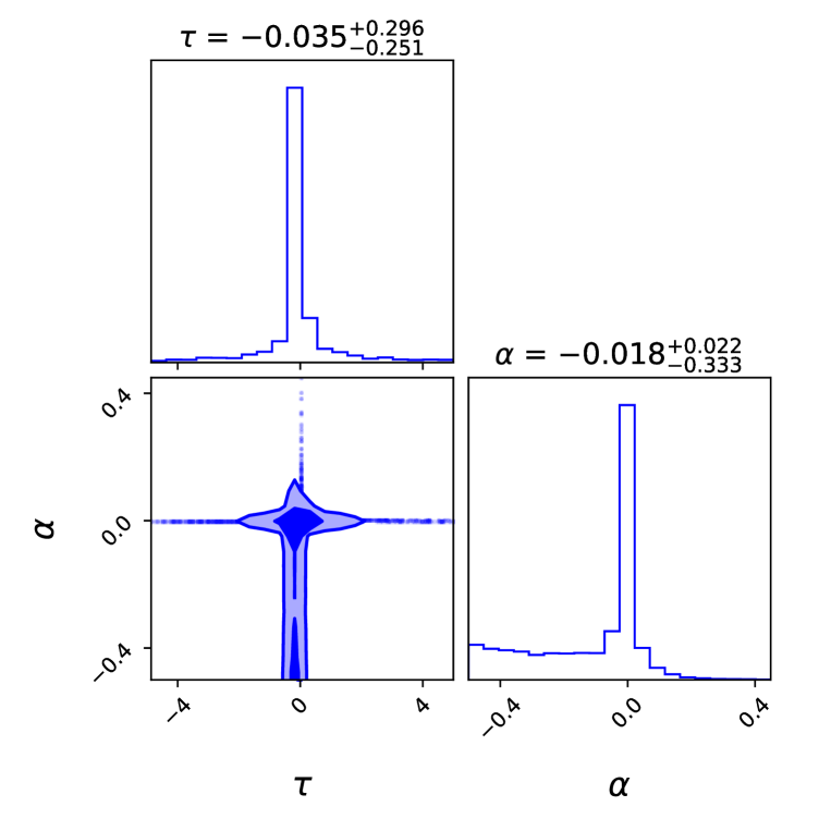
Figure 1: The marginalized 68% and 90% credible regions for the parameters of the null hypothesis of the observed time lags being only due to intrinsic emission. The marginalized best-fit estimates for $\tau$ and $\alpha$ are depicted in the figure.

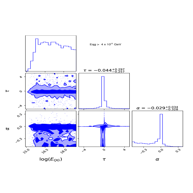
Figure 2: The marginalized 68% and 90% credible regions for the intrinsic lag along with the linear LIV model, corresponding to $n=1$ in Eq. 4. Since, no closed contour for $E_{QG}$ is obtained, we only set lower limits on $E_{QG}$ , given by $E_{QG}>4\times 10^{15}$ GeV at 95% c.l. For this figure, we use GPR to characterize the expansion history.

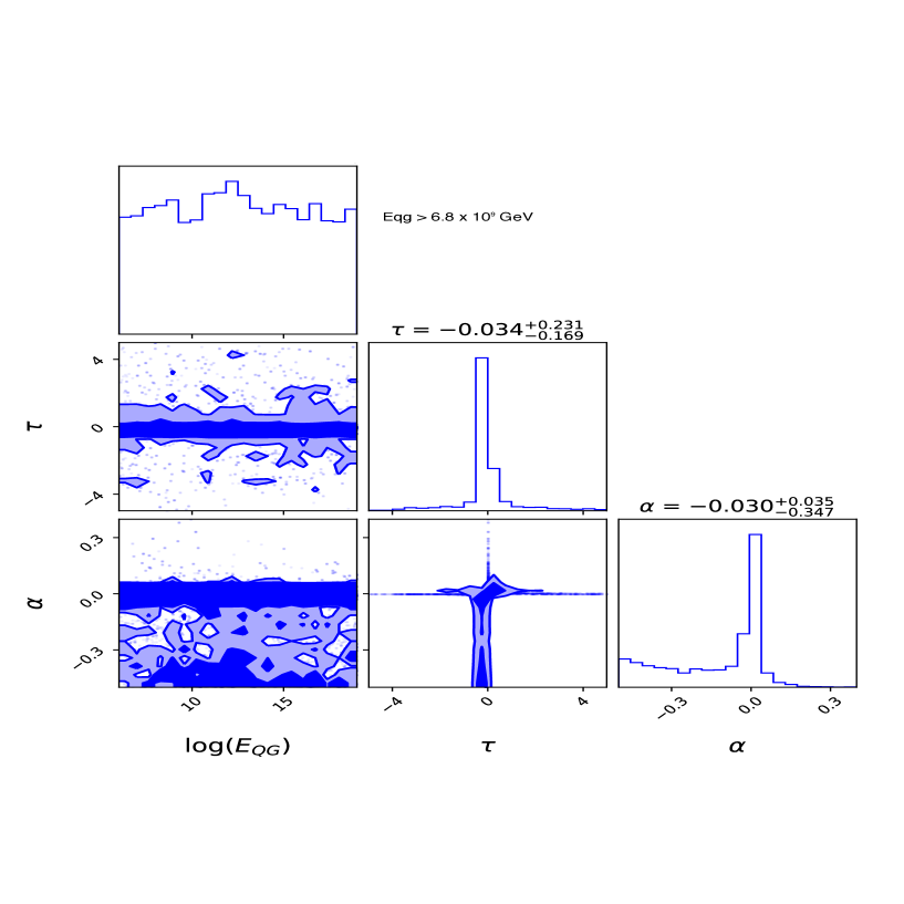
Figure 3: The marginalized 68% and 90% credible regions for the intrinsic lag along with the quadratic LIV model, corresponding to $n=2$ in Eq. 4. Since, no closed contour for $E_{QG}$ is obtained (similar to Fig. 2), we only set lower limits on $E_{QG}$, given by $E_{QG}>6.8\times 10^{9}$ GeV at 95% c.l. For this figure, we use GPR to characterize the expansion history.

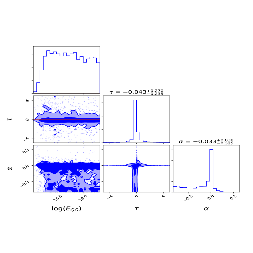
Figure 4: The marginalized 68% and 90% credible regions for the intrinsic lag along with the linear LIV model, corresponding to $n=1$ in Eq. 4 and using the $\Lambda$CDM model to characterize the expansion history. The 95% c.l. lower limit on $E_{QG}$ is given by $E_{QG}>3.3\times 10^{15}$ GeV.

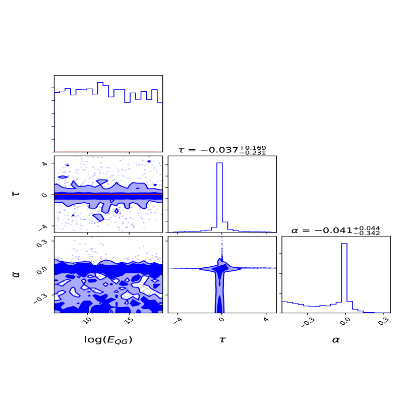
Figure 5: The marginalized 68% and 90% credible regions for the intrinsic lag along with the quadratic LIV model, corresponding to $n=2$ in Eq. 4 and using the $\Lambda$CDM model to characterize the expansion history. The 95% c.l. lower limit on $E_{QG}$ is given by $E_{QG}>10^{9}$ GeV.

	No LIV	Expansion history	(n=1) LIV	(n=2) LIV
$\chi^{2}/\rm{DOF}$	Chronometers	55.8/44	51.3/43	52.6/43
Bayes Factor		-	0.3	1.1
$\chi^{2}/\rm{DOF}$	$\Lambda$CDM	55.8/44	50.6/43	50.2/43
Bayes Factor		-	0.3	1.03

Table 2: Bayesian statistical significance of the two LIV models as compared to the null hypothesis of only intrinsic emission. We also provide the $\chi^{2}$/DOF for all the three models, where DOF is equal to the total number of data points minus the number of free parameters. The first two rows show the results when cosmic chronometers were used to characterize the expansion history and the last two rows contain the results for $\Lambda$CDM. The Bayes factor shows negligible evidence for LIV for both the models and choices of expansion history. The $\chi^{2}$/DOF show reasonable fits for all the models.

III.3 Sensitivity to prior choices

We should point out that for our analyses we have used uniform priors on all the three parameters. The prior range for $\log(E_{QG}$ (GeV)) $\in[6,19]$ is a conservative choice. Although some works have obtained limits on $E_{QG}<10^{19}$ GeV, these involve simplifying assumptions on the intrinsic time lags and hence we do not consider this. Despite this conservative choice, we do not get closed contours for $E_{QG}$ in both the LIV analyses. We should also note that a few works have also obtained 95% c.l. lower limits on $E_{QG}$ greater than the Planck scale Abdo et al. (2009); Vasileiou et al. (2013, 2015). However, given that some works Xu and Ma (2016a, b); Wei et al. (2017a) (see also references in A21) have argued for evidence for LIV, contradicting the above lower limits, it is important to test for signatures of LIV in order to verify these results. We did check that choosing a Gaussian prior on $\tau$ with a mean equal to zero and $\sigma=0.3$ does not qualitatively change our conclusions. Therefore, to summarize, although a detailed sensitivity studies of our results as a function of prior choices is beyond the scope of this work, we have shown that our results do not change with a Gaussian prior on $\tau$. Furthermore, since we not get closed contours for $E_{QG}$ despite choosing a wide prior range, they would not change our results if we truncate the prior.

IV Conclusions

In a recent work, X22 carried out a search for LIV from the spectral lags of 46 short GRBs between two fixed energy intervals in the source frame: 120-250 keV and 15-70 keV.

In this work, we carried out an independent search for LIV using the same spectral lag data following the methodology described in our previous work Agrawal et al. (2021). Instead of assuming a constant model for the intrinsic emission as in X22, we used the same power-law model as a function of energy for the intrinsic emission as in A21. We parameterized the expansion history of the universe (needed to evaluate the LIV-induced lag) in a model-independent way using cosmic chronometers as well as using a flat $\Lambda$CDM cosmology. We searched for both linear and quadratic LIV.

The marginalized credible intervals for the parameters of all three of our models obtained using chronometers to characterize the expansion history can be found in Fig. 1, Fig. 2, and Fig. 3. Since we do not get closed contours for $E_{QG}$, we set 95% c.l. lower limits. We find that $E_{QG}>4\times 10^{15}$ GeV and $E_{QG}>6.8\times 10^{9}$ for linear LIV and quadratic LIV, respectively. The results obtained using $\Lambda$CDM to calculate the expansion history are also comparable, viz $E_{QG}>4\times 10^{15}$ GeV and $E_{QG}>6.8\times 10^{9}$ for linear LIV and quadratic LIV, respectively. The corresponding plots assuming $\Lambda$CDM can be found in Fig. 4 and Fig. 5 and in Table 2.

The corresponding 95% c.l. lower limits obtained in X22 were $\mathcal{O}(10^{15}-10^{17})$ GeV and $\mathcal{O}(10^{6})$ GeV, for linear and quadratic LIV model respectively, depending on the sign of the LIV term. We note however that X22 have obtained closed contours for the term which parameterizes the effect of LIV. Therefore, the one-sided lower limits reported in X22 do not adhere to the upper/lower limit estimation procedure recommended in PDG, and they should have instead reported the bound confidence intervals for $E_{QG}$. There is a similar issue with many previous works in literature which have reported only one-sided lower limit on $E_{QG}$, despite obtaining bound confidence intervals on $E_{QG}$ which are less than the Planck scaleWei et al. (2017a); Pan et al. (2020); Du et al. (2021). For the stacked analysis in A21 using the datasets in  Ellis et al. (2006); Wei et al. (2017a); Du et al. (2021), we did not get a closed contour for $E_{QG}$ for the linear LIV model (See Table 2 in A21). For this case the 68% lower limit is given by $E_{QG}>10^{16}$ GeV. Therefore, our 95% c.l. lower limit is comparable in magnitude to the corresponding result in A21.

The $\chi^{2}$/DOF for all the three models are close to one indicating that the current models don’t help to conclude on the presence of any of the effects investigated. We find that the Bayes factors are close to one, indicating that there is no evidence that spectral lags are induced due to LIV.

We finally point out some limitations of our analysis. We have not considered the uncertainty in the cosmological parameters or in the chronometer $H(z)$ measurements. Although, previous works have shown that the results on LIV are insensitive to the underlying cosmological model Pan et al. (2015); Biesiada and Piórkowska (2009), it is still important to propagate the uncertainties due to Cosmology. Another limitation is that we have considered a flat spectrum for both the lower and upper energy intervals to calculate $E$ and $E_{0}$. Although this ansatz has been used in all works on LIV, for a more accurate estimate one must use the fitted Band spectrum parameters, to get the average value of $E$ and $E_{0}$ along with its uncertainties. This will be implemented in a future work. Finally, the main limiting source of systematic, which has been the bane of all LIV searches is the uncertainty due to the intrinsic GRB emission mechanism Wei and Wu (2021). The main assumption in this work is that the power-law model used for the intrinsic emission mechanism (or the constant model used in X22 and other works) would adequately fit all GRBs in our sample with the same parameters. However, given the diversity in the light curves of GRBs, there is no guarantee that this assumption is correct. In the future one may need to do a separate analysis per GRB (based on the prompt or afterglow spectra) and apply phenomenological models such as that used in  Chang et al. (2012) or incorporate the luminosity-lag correlation Vardanyan et al. (2022) to model the intrinsic emission. Nevertheless, for these reasons it is more straightforward to carry out LIV analysis on a single GRB as done in  Du et al. (2021); Wei et al. (2017a).

We note that our limits are not as sensitive as the MAGIC limit (from GRB 1900114C), which is $\mathcal{O}(10^{19}GeV)$ and $\mathcal{O}(10^{10}GeV)$ for linear and quadratic LIV models, respectively Acciari et al. (2020) or the Fermi-LAT limit of $7.6\times 10^{19}$/ $10^{11}$ GeV for linear/quadratic LIV models obtained using four GRBs Vasileiou et al. (2013). The sensitivity to LIV increases at higher photon energies. Since the MAGIC limit Acciari et al. (2020) is obtained from the detection of TeV gamma rays (as compared to keV energy GRBs in our work), their limit is the more stringent. However, this result also involves assumptions about the intrinsic spectral and temporal emission properties, for which conservative choices have been made in Ref. Acciari et al. (2020). Similarly the limits in Ref. Vasileiou et al. (2013) were also obtained using GeV observations of GRBs, and hence are more stringent than those in our work. This work used three independent statistical methods. All these methods do involve assumptions regarding possible source-intrinsic spectral-evolution effects, for which conservative choices have been made Vasileiou et al. (2013). Therefore, to summarize, although the aforementioned works do not posit any parametric model for the intrinsic time delay (as in our analysis), they do need to assume a model for the intrinsic spectral and temporal evolution in order to obtain limits in $E_{QG}$.)

We finally note that the broad Bayesian methodology used in this work to search for LIV can be easily applied to GRBs with spectral lag measurements in GeV energy range as well as non-GRB sources, for which spectral lag measurements are available.

References

- Xiao et al. (2022) S. Xiao, S.-L. Xiong, Y. Wang, S.-N. Zhang, H. Gao, Z. Zhang, C. Cai, Q.-B. Yi, Y. Zhao, Y.-L. Tuo, et al., Astrophys. J. Lett. 924, L29 (2022).
- Amelino-Camelia et al. (1998a) G. Amelino-Camelia, J. Ellis, N. E. Mavromatos, D. V. Nanopoulos, and S. Sarkar, Nature (London) 395, 525 (1998a).
- Addazi et al. (2022) A. Addazi et al., Prog. Part. Nucl. Phys. 125, 103948 (2022), eprint 2111.05659.
- Amelino-Camelia et al. (1998b) G. Amelino-Camelia, J. Ellis, N. E. Mavromatos, D. V. Nanopoulos, and S. Sarkar, Nature (London) 393, 763 (1998b), eprint astro-ph/9712103.
- Ellis et al. (2003) J. Ellis, N. E. Mavromatos, D. V. Nanopoulos, and A. S. Sakharov, Astron. & Astrophys. 402, 409 (2003), eprint astro-ph/0210124.
- Ellis et al. (2006) J. Ellis, N. E. Mavromatos, D. V. Nanopoulos, A. S. Sakharov, and E. K. G. Sarkisyan, Astroparticle Physics 25, 402 (2006), eprint astro-ph/0510172.
- Abdo et al. (2009) A. A. Abdo, M. Ackermann, M. Ajello, K. Asano, W. B. Atwood, M. Axelsson, L. Baldini, J. Ballet, G. Barbiellini, M. G. Baring, et al., Nature (London) 462, 331 (2009), eprint 0908.1832.
- Chang et al. (2016) Z. Chang, X. Li, H.-N. Lin, Y. Sang, P. Wang, and S. Wang, Chinese Physics C 40, 045102 (2016), eprint 1506.08495.
- Vasileiou et al. (2013) V. Vasileiou, A. Jacholkowska, F. Piron, J. Bolmont, C. Couturier, J. Granot, F. W. Stecker, J. Cohen-Tanugi, and F. Longo, Phys. Rev. D 87, 122001 (2013), eprint 1305.3463.
- Vasileiou et al. (2015) V. Vasileiou, J. Granot, T. Piran, and G. Amelino-Camelia, Nature Physics 11, 344 (2015).
- Zhang and Ma (2015) S. Zhang and B.-Q. Ma, Astroparticle Physics 61, 108 (2015), eprint 1406.4568.
- Liu and Ma (2018) Y. Liu and B.-Q. Ma, European Physical Journal C 78, 825 (2018), eprint 1810.00636.
- Pan et al. (2015) Y. Pan, Y. Gong, S. Cao, H. Gao, and Z.-H. Zhu, Astrophys. J. 808, 78 (2015), eprint 1505.06563.
- Xu and Ma (2016a) H. Xu and B.-Q. Ma, Physics Letters B 760, 602 (2016a), eprint 1607.08043.
- Xu and Ma (2016b) H. Xu and B.-Q. Ma, Astroparticle Physics 82, 72 (2016b), eprint 1607.03203.
- Wei and Wu (2017) J.-J. Wei and X.-F. Wu, Astrophys. J. 851, 127 (2017), eprint 1711.09185.
- Ganguly and Desai (2017) S. Ganguly and S. Desai, Astroparticle Physics 94, 17 (2017), eprint 1706.01202.
- Ellis et al. (2019) J. Ellis, R. Konoplich, N. E. Mavromatos, L. Nguyen, A. S. Sakharov, and E. K. Sarkisyan-Grinbaum, Phys. Rev. D 99, 083009 (2019), eprint 1807.00189.
- Wei (2019) J.-J. Wei, Mon. Not. R. Astron. Soc. 485, 2401 (2019), eprint 1905.03413.
- Du et al. (2021) S.-S. Du, L. Lan, J.-J. Wei, Z.-M. Zhou, H. Gao, L.-Y. Jiang, B.-B. Zhang, Z.-K. Liu, X.-F. Wu, E.-W. Liang, et al., Astrophys. J. 906, 8 (2021), eprint 2010.16029.
- Pan et al. (2020) Y. Pan, J. Qi, S. Cao, T. Liu, Y. Liu, S. Geng, Y. Lian, and Z.-H. Zhu, Astrophys. J. 890, 169 (2020), eprint 2001.08451.
- Acciari et al. (2020) V. A. Acciari et al. (MAGIC, Armenian Consortium: ICRANet-Armenia at NAS RA, A. Alikhanyan National Laboratory, Finnish MAGIC Consortium: Finnish Centre of Astronomy with ESO), Phys. Rev. Lett. 125, 021301 (2020), eprint 2001.09728.
- Zou et al. (2018) X.-B. Zou, H.-K. Deng, Z.-Y. Yin, and H. Wei, Physics Letters B 776, 284 (2018), eprint 1707.06367.
- Agrawal et al. (2021) R. Agrawal, H. Singirikonda, and S. Desai, JCAP 2021, 029 (2021), eprint 2102.11248.
- Bartlett et al. (2021) D. J. Bartlett, H. Desmond, P. G. Ferreira, and J. Jasche, Phys. Rev. D 104, 103516 (2021), eprint 2109.07850.
- Wei and Wu (2021) J.-J. Wei and X.-F. Wu, Frontiers of Physics 16, 44300 (2021), eprint 2102.03724.
- Liu et al. (2022) Z.-K. Liu, B.-B. Zhang, and Y.-Z. Meng, arXiv e-prints arXiv:2202.09999 (2022), eprint 2202.09999.
- Kumar and Zhang (2015) P. Kumar and B. Zhang, Physics Reports 561, 1 (2015), eprint 1410.0679.
- Huang et al. (2022) Y. Huang, S. Hu, S. Chen, M. Zha, C. Liu, Z. Yao, Z. Cao, and T. L. Experiment, GRB Coordinates Network 32677, 1 (2022).
- Singh and Desai (2022) A. Singh and S. Desai, JCAP 2022, 010 (2022), eprint 2108.00395.
- Kouveliotou et al. (1993) C. Kouveliotou, C. A. Meegan, G. J. Fishman, N. P. Bhat, M. S. Briggs, T. M. Koshut, W. S. Paciesas, and G. N. Pendleton, Astrophys. J. Lett. 413, L101 (1993).
- Woosley and Bloom (2006) S. E. Woosley and J. S. Bloom, Ann. Rev. Astron. Astrophys. 44, 507 (2006), eprint astro-ph/0609142.
- Nakar (2007) E. Nakar, Physics Reports 442, 166 (2007), eprint astro-ph/0701748.
- Kulkarni and Desai (2017) S. Kulkarni and S. Desai, Astrophys. and Space Science 362, 70 (2017), eprint 1612.08235.
- Bhave et al. (2022) A. Bhave, S. Kulkarni, S. Desai, and P. K. Srijith, Astrophys. and Space Science 367, 39 (2022), eprint 1708.05668.
- Li et al. (2004) T.-P. Li, J.-L. Qu, H. Feng, L.-M. Song, G.-Q. Ding, and L. Chen, ChJAA 4, 583 (2004), eprint astro-ph/0407458.
- Xiao et al. (2021) S. Xiao, S. L. Xiong, S. N. Zhang, L. M. Song, F. J. Lu, Y. Huang, C. Cai, Q. B. Yi, X. Y. Song, W. Chen, et al., Astrophys. J. 920, 43 (2021).
- Krishak and Desai (2020) A. Krishak and S. Desai, JCAP 2020, 006 (2020), eprint 2003.10127.
- Wei et al. (2017a) J.-J. Wei, B.-B. Zhang, L. Shao, X.-F. Wu, and P. Mészáros, Astrophys. J. Lett. 834, L13 (2017a), eprint 1612.09425.
- Shao et al. (2017) L. Shao, B.-B. Zhang, F.-R. Wang, X.-F. Wu, Y.-H. Cheng, X. Zhang, B.-Y. Yu, B.-J. Xi, X. Wang, H.-X. Feng, et al., Astrophys. J. 844, 126 (2017), eprint 1610.07191.
- Perennes et al. (2020) C. Perennes, H. Sol, and J. Bolmont, Astron. & Astrophys. 633, A143 (2020), eprint 1911.10377.
- Aghanim et al. (2020) N. Aghanim et al. (Planck), Astron. Astrophys. 641, A6 (2020), eprint 1807.06209.
- Abdalla et al. (2022) E. Abdalla et al., JHEAp 34, 49 (2022), eprint 2203.06142.
- Trotta (2017) R. Trotta, ArXiv e-prints (2017), eprint 1701.01467.
- Sharma (2017) S. Sharma, Ann. Rev. Astron. Astrophys. 55, 213 (2017), eprint 1706.01629.
- Kerscher and Weller (2019) M. Kerscher and J. Weller, SciPost Physics Lecture Notes 9 (2019), eprint 1901.07726.
- Bromberg et al. (2013) O. Bromberg, E. Nakar, T. Piran, and R. Sari, Astrophys. J. 764, 179 (2013), eprint 1210.0068.
- Evans et al. (2009) P. A. Evans, A. P. Beardmore, K. L. Page, J. P. Osborne, P. T. O’Brien, R. Willingale, R. L. C. Starling, D. N. Burrows, O. Godet, L. Vetere, et al., Mon. Not. R. Astron. Soc. 397, 1177 (2009), eprint 0812.3662.
- von Kienlin et al. (2020) A. von Kienlin, C. A. Meegan, W. S. Paciesas, P. N. Bhat, E. Bissaldi, M. S. Briggs, E. Burns, W. H. Cleveland, M. H. Gibby, M. M. Giles, et al., Astrophys. J. 893, 46 (2020), eprint 2002.11460.
- Band et al. (1993) D. Band, J. Matteson, L. Ford, B. Schaefer, D. Palmer, B. Teegarden, T. Cline, M. Briggs, W. Paciesas, G. Pendleton, et al., Astrophys. J. 413, 281 (1993).
- Wei et al. (2017b) J.-J. Wei, X.-F. Wu, B.-B. Zhang, L. Shao, P. Mészáros, and V. A. Kostelecký, Astrophys. J. 842, 115 (2017b), eprint 1704.05984.
- Fishman (1995) G. J. Fishman, PASP 107, 1145 (1995).
- Vardanyan et al. (2022) V. Vardanyan, V. Takhistov, M. Ata, and K. Murase, arXiv e-prints arXiv:2212.02436 (2022), eprint 2212.02436.
- Jacob and Piran (2008) U. Jacob and T. Piran, JCAP 1, 031 (2008), eprint 0712.2170.
- Seikel et al. (2012) M. Seikel, C. Clarkson, and M. Smith, JCAP 1206, 036 (2012), eprint 1204.2832.
- Jimenez and Loeb (2002) R. Jimenez and A. Loeb, Astrophys. J. 573, 37 (2002), eprint astro-ph/0106145.
- Singirikonda and Desai (2020) H. Singirikonda and S. Desai, European Physical Journal C 80, 694 (2020), eprint 2003.00494.
- Bora and Desai (2021) K. Bora and S. Desai, JCAP 2021, 052 (2021), eprint 2104.00974.
- Vagnozzi et al. (2021) S. Vagnozzi, A. Loeb, and M. Moresco, Astrophys. J. 908, 84 (2021), eprint 2011.11645.
- Holanda et al. (2022) R. F. L. Holanda, K. Bora, and S. Desai, European Physical Journal C 82, 526 (2022), eprint 2105.10988.
- Moresco et al. (2022) M. Moresco, L. Amati, L. Amendola, S. Birrer, J. P. Blakeslee, M. Cantiello, A. Cimatti, J. Darling, M. Della Valle, M. Fishbach, et al., arXiv e-prints arXiv:2201.07241 (2022), eprint 2201.07241.
- Rosati et al. (2015) G. Rosati, G. Amelino-Camelia, A. Marcianò, and M. Matassa, Phys. Rev. D 92, 124042 (2015), eprint 1507.02056.
- Bolmont et al. (2022) J. Bolmont, S. Caroff, M. Gaug, A. Gent, A. Jacholkowska, D. Kerszberg, C. Levy, T. Lin, M. Martinez, L. Nogués, et al., Astrophys. J. 930, 75 (2022), eprint 2201.02087.
- Krishak et al. (2020) A. Krishak, A. Dantuluri, and S. Desai, JCAP 2020, 007 (2020), eprint 1906.05726.
- Bhagvati and Desai (2021) S. Bhagvati and S. Desai, JCAP 2021, 022 (2021), eprint 2106.06724.
- Speagle (2020) J. S. Speagle, Mon. Not. R. Astron. Soc. (2020), eprint 1904.02180.
- Group et al. (2020) P. D. Group, P. Zyla, R. Barnett, J. Beringer, O. Dahl, D. Dwyer, D. Groom, C.-J. Lin, K. Lugovsky, E. Pianori, et al., Progress of Theoretical and Experimental Physics 2020, 083C01 (2020).
- Biesiada and Piórkowska (2009) M. Biesiada and A. Piórkowska, Classical and Quantum Gravity 26, 125007 (2009), eprint 1008.2615.
- Chang et al. (2012) Z. Chang, Y. Jiang, and H.-N. Lin, Astroparticle Physics 36, 47 (2012), eprint 1201.3413.