Production of three isolated photons in the parton Reggeization approach at high energies

Abstract

We study a large-$p_{T}$ three-photon production in proton-proton collisions at the LHC. We use the leading order (LO) approximation of the parton Reggeization approach consistently merged with the next-to-leading order corrections originated from the emission of additional jet. For numerical calculations we use the parton-level generator KaTie and modified KMR-type unintegrated parton distribution functions which satisfy exact normalization conditions for arbitrary $x$. We compare our prediction with data from ATLAS collaboration at the center-of-mass energy $\sqrt{s}=8$ TeV. We find that the inclusion of the real next-to-leading-order corrections leads to a good agreement between our predictions and data with the same accuracy as for the next-to-next-to-leading calculations based on the collinear parton model of QCD. At higher energies ($\sqrt{s}=13$ and 27 TeV) parton Reggeization approach predicts larger cross sections, up to $\sim 15$ % and $\sim 30$ %, respectively.

I Introduction

The recent experimental data for a large-$p_{T}$ multi-photon production at the Tevatron CDF1 ; CDF2 and LHC LHC71 ; LHC72 ; LHC8 at the energy range from 1.96 TeV up to 8 TeV are extensively studied in the collinear parton model (CPM) of perturbative quantum chromodynamics (QCD) beyond the leading-order (LO) accuracy in strong-coupling constant, $\alpha_{S}$, i.e. at the next-to-leading-order (NLO) NLO21 ; NLO31 ; NLO32 and even at next-to-next-to-leading-order (NNLO) NNLO21 ; NNLO22 ; NNLO31 ; NNLO32 . The high-order calculations for two-photon or three-photon production in CPM of QCD provide rather bad agreement with data at the level of NLO accuracy. For example, NLO QCD calculations strongly underestimate, by factor 2 or even more, recent data from ATLAS Collaboration at $\sqrt{s}=8$ TeV LHC8 for three-photon production. The inclusion of additional contribution from parton-shower mechanism and hadronization effects NLO31 to the NLO calculations increase theoretical prediction but they are being yet far from measured cross sections.

Inclusion of the NNLO QCD corrections for two-photon production NNLO21 and three-photon production NNLO31 ; NNLO32 eliminates the existing discrepancy with respect to NLO QCD predictions. However, for three-photon production the agreement with data is not so good as for two-photon production and it is achieved when hard scale parameter $\mu$ should be taken very small relatively usual used value NNLO31 .

In CPM of QCD we neglect the transverse momenta of initial-state partons in hard-scattering amplitudes that is a correct assumption for the fully inclusive observables, such as $p_{T}$-spectra of single prompt photons or jets, where their large transverse momentum defines single hard scale of the process, $\mu\sim p_{T}$. The corrections breaking the collinear factorization are shown to be suppressed by powers of the hard scale Collins .

The multi-photon large-$p_{T}$ production is multi-scale hard process in which using the simple collinear picture of initial state radiation may be a bad approximation. In the present paper, we calculate different multi-scale variables in three-photon production from a point of view of High-Energy Factorization (HEF) or $k_{T}-$factorization, which initially has been introduced as a resummation tool for $\ln(\sqrt{s}/\mu)$-enhanced corrections to the hard-scattering coefficients in CPM, where invariants $\sqrt{s}$ referees to the total energy of process. We use the parton Reggeization approach (PRA) which is a version of HEF formalism, based on the modified Multi-Regge Kinematics (mMRK) approximation for QCD scattering amplitudes. This approximation is accurate both in the collinear limit, which drives the Transverse-Momentum-Dependent (TMD) factorization Collins and in the high-energy (Multi-Regge) limit, which is important for Balitsky-Fadin-Kuraev-Lipatov(BFKL) BFKL1 ; BFKL2 ; BFKL3 ; BFKL4 resummation of $\ln(\sqrt{s}/\mu)$-enhanced effects.

In the same manner of the PRA, we have studied previously one-photon production  one-photon , two-photon production two-photon and photon plus jet production  photon-jet in proton-(anti)proton collisions at the Tevatron and the LHC. At the present paper we study a production or three isolated photons at the LHC. Preliminary, our predictions has been presented as short note at DIS2021 Conference, see Ref. SaleevDIS . The similar study of three-photon production in the $k_{T}-$factorization approach was published recently in Ref. three-photon , where authors compared predictions obtained with different unPDFs KMR ; WMR ; PB1 ; PB2 that is compliment to our study in PRA SaleevDIS .

The paper has the following structure, in Section II the relevant basics of the PRA formalism are outlined. In the Section III we overview Monte-Carlo (MC) parton-level event generator KaTie and the relation between PRA and KaTie MC calculations for tree-level amplitudes. In the Section IV we compare obtained in the PRA results with the recent ATLAS LHC8 data as well as with theoretical predictions obtained in NNLO calculations of CPM NNLO31 ; NNLO32 . Our conclusions are summarized in the Section V.

II Parton Reggeization Approach

The PRA is based on high-energy factorization for hard processes in the Multi-Regge kinematics. The basic ingredients of PRA are $k_{T}-$dependent factorization formula, unintegrated parton distribution functions (unPDF’s) and gauge-invariant amplitudes with off-shell initial-state partons. The first one is proved in the leading-logarithmic-approximation of high-energy QCD KTfactorization1 ; KTfactorization2 , the second one is constructed in the same manner as it was suggested by Kimber, Martin, Ryskin and Watt KMR ; WMR , but with sufficient revision NefedovSaleev2020 . The off-shell amplitudes are derived using the Lipatov’s Effective Field Theory (EFT) of Reggeized gluons Lipatov95 and Reggeized quarks LipatovVyazovsky . The brief description of LO in $\alpha_{S}$ approximation of PRA is presented below. More details can be found in Refs. NSS2013 ; NKS2017 , the inclusion of real NLO corrections in the PRA was studied in Ref. NKS2017 , the development of PRA in the full one-loop NLO approximation was further discussed in PRANLO1 ; PRANLO2 ; PRANLO3 .

Factorization formula of PRA in LO approximation for the process $p+p\to{\cal Y}+X$, can be obtained from factorization formula of the CPM for the auxiliary hard subprocess like $g+g\to q+{\cal Y}+\bar{q}$. For discussed here process of three-photon production, ${\cal Y}=\gamma\gamma\gamma$. In the Ref. NKS2017 the modified Multi-Regge Kinematics (mMRK) approximation for the auxiliary amplitude has been constructed, which correctly reproduces the Multi-Regge and collinear limits of corresponding QCD amplitude. This mMRK-amplitude has $t$-channel factorized form, which allows one to rewrite the cross-section of auxiliary subprocess in a $k_{T}$-factorized form:

$$d\sigma = \sum_{i,\bar{j}}\int\limits_{0}^{1}\frac{dx_{1}}{x_{1}}\int\frac{d^{2}{\bf q}_{T1}}{\pi}\tilde{\Phi}_{i}(x_{1},t_{1},\mu^{2})\int\limits_{0}^{1}\frac{dx_{2}}{x_{2}}\int\frac{d^{2}{\bf q}_{T2}}{\pi}\tilde{\Phi}_{j}(x_{2},t_{2},\mu^{2})\cdot d\hat{\sigma}_{\rm PRA},$$ (1)

where $t_{1,2}=-{\bf q}_{T1,2}^{2}$, the off-shell partonic cross-section $\hat{\sigma}_{\rm PRA}$ in PRA is determined by squared PRA amplitude, $\overline{|{\cal A}_{PRA}|^{2}}$. Despite the fact that four-momenta ($q_{1,2}$) of partons in the initial state of amplitude ${\cal A}_{PRA}$ are off-shell ($q_{1,2}^{2}=-t_{1,2}<0$), the PRA hard-scattering amplitude is gauge-invariant because the initial-state off-shell partons are treated as Reggeized partons of gauge-invariant EFT for QCD processes in Multi-Regge Kinematics (MRK), introduced by L.N. Lipatov in Lipatov95 ; LipatovVyazovsky . The Feynman rules of this EFT are written down in Refs. LipatovVyazovsky ; AntonovLipatov .

The tree-level unPDFs  $\tilde{\Phi}_{i}(x_{1,2},t_{1,2},\mu^{2})$ in Eq. (1) are equal to the convolution of the collinear PDFs $f_{i}(x,\mu^{2})$ and Dokshitzer-Gribov-Lipatov-Altarelli-Parisi (DGLAP) splitting function $P_{ij}(z)$ with the factor $1/t_{1,2}$,

$$\tilde{\Phi}_{i}(x,t,\mu)=\frac{\alpha_{s}(\mu)}{2\pi}\frac{1}{t}\sum\limits_{j=q,\bar{q},g}\int\limits_{x}^{1}dz\ P_{ij}(z){F}_{j}\left(\frac{x}{z},\mu_{F}^{2}\right),$$ (2)

where $F_{i}(x,\mu_{F}^{2})=xf_{j}(x,\mu_{F}^{2})$. Here and above we put $\mu_{F}=\mu_{R}=\mu$. Consequently, the cross-section (1) with such unPDFs contains the collinear divergence at $t_{1,2}\to 0$ and infrared (IR) divergence at $z_{1,2}\to 1$.

To resolve collinear divergence problem of $\tilde{\Phi}_{i}(x,t,\mu)$ we require that modified unPDF ${\Phi}_{i}(x,t,\mu)$ should be satisfied exact normalization condition:

$$\int\limits_{0}^{\mu^{2}}dt\Phi_{i}(x,t,\mu^{2})={F}_{i}(x,\mu^{2}),$$ (3)

which is equivalent to:

$$\Phi_{i}(x,t,\mu^{2})=\frac{d}{dt}\left[T_{i}(t,\mu^{2},x){F}_{i}(x,t)\right],$$ (4)

where $T_{i}(t,\mu^{2},x)$ is usually referred to as Sudakov form-factor, satisfying the boundary conditions $T_{i}(t=0,\mu^{2},x)=0$ and $T_{i}(t=\mu^{2},\mu^{2},x)=1$. Such a way, modified unPDF can be written as follows from KMR model:

$$\Phi_{i}(x,t,\mu)=\frac{\alpha_{s}(\mu)}{2\pi}\frac{T_{i}(t,\mu^{2},x)}{t}\sum\limits_{j=q,\bar{q},g}\int\limits_{x}^{1}dz\ P_{ij}(z){F}_{j}\left(\frac{x}{z},t\right)\theta\left(\Delta(t,\mu)-z\right).$$ (5)

Here, we resolved also IR divergence taking into account observation that the mMRK expression gives a reasonable approximation for the exact matrix element only in the rapidity-ordered part of the phase-space. From this requirement, the following cutoff on $z_{1,2}$ can be derived: $z_{1,2}<1-\Delta_{KMR}(t_{1,2},\mu^{2}),$ where $\Delta_{KMR}(t,\mu^{2})=\sqrt{t}/(\sqrt{\mu^{2}}+\sqrt{t})$ is the KMR-cutoff function KMR .

The solution for Sudakov form-factor in Eq. (4) has been obtained in Ref. NefedovSaleev2020 :

$$T_{i}(t,\mu^{2},x)=\exp\left[-\int\limits_{t}^{\mu^{2}}\frac{dt^{\prime}}{t^{\prime}}\frac{\alpha_{s}(t^{\prime})}{2\pi}\left(\tau_{i}(t^{\prime},\mu^{2})+\Delta\tau_{i}(t^{\prime},\mu^{2},x)\right)\right]$$ (6)

with

$$\tau_{i}(t,\mu^{2}) = \sum\limits_{j}\int\limits_{0}^{1}dz\ zP_{ji}(z)\theta(\Delta(t,\mu^{2})-z),$$

$$\Delta\tau_{i}(t,\mu^{2},x) = \sum\limits_{j}\int\limits_{0}^{1}dz\ \theta(z-\Delta(t,\mu^{2}))\left[zP_{ji}(z)-\frac{{F}_{j}\left(\frac{x}{z},t\right)}{{F}_{i}(x,t)}P_{ij}(z)\theta(z-x)\right].$$

Let us summarize important differences between the Sudakov form-factor obtained in our mMRK approach (6) and in the KMR approach  KMR . At first, the Sudakov form-factor (6) contains the $x-$depended $\Delta\tau_{i}$-term in the exponent which is needed to preserve exact normalization condition for arbitrary $x$ and $\mu$. The second one is a numerically-important difference that in our mMRK approach the rapidity-ordering condition is imposed both on quarks and gluons, while in KMR approach it is imposed only on gluons.

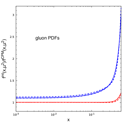
Figure 3: Ratio for integrated over transverse momentum unPDF to parent collinear PDF for gluon as function of $x$ at different choice of hard scale $\mu^{2}=10^{4},6\times 10^{4},10^{5}$ GeV² which correspond to dashed, solid and dotted-dashed lines. Blue lines are obtained in original KMR model KMR ; WMR and red lines are obtained in our modified approach NefedovSaleev2020 .

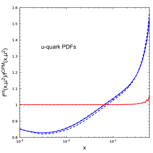
Figure 4: Ratio for integrated over transverse momentum unPDF to parent collinear PDF for valence $u-$quark as function of $x$ at different choice of hard scale $\mu^{2}=10^{4},6\times 10^{4},10^{5}$ GeV², which correspond to dashed, solid and dotted-dashed lines. Blue lines are obtained in original KMR model KMR ; WMR and red lines are obtained in our modified approach NefedovSaleev2020 .

To illustrate differences between unPDFs at large $x$, obtained in original KMR KMR ; WMR model and in our modified approach NefedovSaleev2020 , we plot ratios for integrated over transverse momentum unPDFs to parent collinear PDFs for gluon and $u-$quark as function of $x$ at different choice of hard scale $\mu$ in Figures 3 and 4, correspondingly.

In contrast to most of studies in the $k_{T}$-factorization, the gauge-invariant matrix elements with off-shell initial-state partons (Reggeized quarks and gluons) from Lipatov’s EFT Lipatov95 ; LipatovVyazovsky allow one to study arbitrary processes involving non-Abelian structure of QCD without violation of Slavnov-Taylor identities due to the nonzero virtuality of initial-state partons. This approach, together with KMR-type unPDFs gives stable and consistent results in a wide range of phenomenological applications, which include the description of the angular correlations of dijets NSS2013 , charmed Maciula:2016wci ; Karpishkov:2014epa and bottom-flavored NKS2017 ; Karpishkov:2016hnx mesons, charmonia Saleev:2012hi ; He:2019qqr as well as some other examples.

III Details of numerical calculations

The first step of calculations in PRA is generation of amplitudes of relevant off-mass shell partonic processes by Feynman rules of Lipatov’s EFT. It can be done using a model file ReggeQCD ReggeQCD for FeynArts tool hahn . In the Fig. 1, the total set of 13 Feynman diagrams for LO process

$$Q\bar{Q}\to\gamma\gamma\gamma$$ (7)

obtained with ReggeQCD is shown. The number of EFT diagrams for NLO in $\alpha_{S}$ involved in our study process

$$QR\to q\gamma\gamma\gamma$$ (8)

is getting too large for analytical calculation. In Fig. 2, the full gauge invariant set of 40 Feynman diagrams is shown. To proceed next step, we should analytically calculate squared off-shell amplitudes and perform a numerical calculation using factorization formula (1) with modified unPDFs (5). At present, we can do it with required numerical accuracy only for $2\to 2$ and $2\to 3$ off-shell parton processes. To calculate contributions from $2\to 4$ processes with initial Reggeized partons we use parton-level generator KaTie katie .

A few years ago, a new approach to derive gauge-invariant scattering amplitudes with off-shell initial-state partons for high-energy scattering, using the spinor-helicity techniques and BCFW-like recursion relations for such amplitudes has been introduced in the Refs. hameren1 ; hameren2 . Some time later the MC parton-level event generator KaTie katie has been developed to provide calculations for hadron scattering processes that can deal with partonic initial-state momenta with an explicit transverse momentum dependence causing them to be space-like. The formalism  hameren1 ; hameren2 for numerical generation of off-shell amplitudes is equivalent to the results of Lipatov’s EFT at the tree level NSS2013 ; NKS2017 ; kutak . We should note here, that for the generalization of the formalism to full NLO level PRANLO1 ; PRANLO2 , the use of explicit Feynman rules and the structure of EFT is more convenient.

Taking in mind above mentioned discussion, the LO contribution of subprocess (7) has been calculated for crosscheck both with KaTie MC generator and using direct integration of analytical squared amplitudes obtained with the help of Feynman rules of Lipatov EFT. All final calculations have been done using MC event generator KaTie katie .

We will neglect NLO contribution in quark-antiquark annihilation channel from subprocesses with additional final gluon

$$Q\bar{Q}\to g\gamma\gamma\gamma,$$ (9)

which should be negligibly small in comparison with main others as in the similar case of NLO CPM calculations. First off all, because the relevant values of involving longitudinal parton momenta are very small ($x<10^{-2}$) at the energy range of the LHC and the gluon density is much larger than the quark (antiquark) ones. Such a way, we avoid difficulties in a calculation of the process (9), which follow from an infra-red divergence, which should be regularized by a contribution from loop correction to the LO process (7) and from double counting between LO (7) and NLO (9) diagrams with emission of an additional gluon. The technique of NLO calculations is still under development in PRA, see discussions in Refs. PRANLO1 ; PRANLO2 ; PRANLO3 .

The next important issue is that a calculation for the process (8) doesn’t contain infra-red and collinear singularities in PRA, after taking in consideration isolation-cone conditions for final photons and partons. Numerical accuracy of total cross section calculations with MC generator KaTie by default is 0.1 % .

IV Results

First of all, we review setup of ATLAS measurements at $\sqrt{s}=8$ TeV LHC8 :

• Photon transverse energies (transverse momenta) (1 is leading photon, 2 is sub-leading photon and 3 is sub-sub-leading photon) $E_{T1}>27$ GeV, $E_{T2}>22$ GeV, $E_{T3}>15$ GeV.

• For rapidity (pseudorapidity) of all photons one has $|\eta_{1,2,3}|<2.37$, excluding the range $1.37<|\eta_{1,2,3}|<1.56$.

• Three-photon invariant mass $M_{123}=M_{3\gamma}>50$ GeV.

• Photon-photon isolation conditions are $\Delta R_{ij}>R_{\gamma\gamma}=0.45$, where $\Delta R_{ij}=\sqrt{(\eta_{i}-\eta_{j})^{2}+(\phi_{i}-\phi_{j})^{2}}$

• Photon-quark isolation conditions are $\Delta R_{iq}>R_{0}=0.40$

To take into account a fragmentation contribution, we use the Frixione smooth photon isolation Frixione . For any angular difference $\Delta R_{iq}$ from each photon, when $\Delta R_{iq}\leq R_{0}$, it is required

$$E_{T}^{iso}(\Delta R_{iq})<E_{T}^{max}\frac{1-\cos(\Delta R{iq})}{1-\cos(R_{0})},$$

where $E_{T}^{max}=10$ GeV, $E_{T}^{iso}=E_{Tq}$.

We test dependence of predicted cross section on choice of factorization ($\mu_{F}$)and renormalization ($\mu_{R}$) scales, which we take equal to each other, $\mu_{F}=\mu_{R}=\mu$. In the Table 1 we compare predictions obtained with $\mu=M_{3\gamma}$ – an invariant mass of the three-photon system and $\mu=E_{T,\sum}=E_{T,1\gamma}+E_{T,2\gamma}+E_{T,3\gamma}$ – a sum of transverse momenta (transverse energies) moduli of photons. Errors indicate upper and lower limits of the cross section obtained due to variation of the hard scale $\mu$ by a factor $\xi=2$ or $\xi=1/2$ around the central value of the hard scale.

Hard scale, $\mu$	$\sigma_{LO}(Q\bar{Q}\to 3\gamma)$ [fb]	$\sigma(QR\to 3\gamma q)$ [fb]	$\sigma_{NLO}$ [fb]
$M_{3\gamma}$	$37.20^{+9.25}_{-7.98}$	$36.94^{-6.14}_{+5.91}$	$73.14^{+4.13}_{-1.07}$
$E_{T,\sum}$	$36.35^{+8.38}_{-9.77}$	$39.26^{-6.29}_{+6.00}$	$75.62^{+3.59}_{-2.39}$

Table 1: PRA predictions for $p+p\to\gamma\gamma\gamma+X$ total cross section at $\sqrt{s}=8$ TeV for the different choice of factorization/renormalization scale ($\mu=\mu_{F}=\mu_{R}$). Errors indicate upper and lower limits of the cross section due to scale uncertainty.

$\sqrt{s}$[TeV]	$\sigma_{LO}(Q\bar{Q}\to 3\gamma)$ [fb]	$\sigma(QR\to 3\gamma q)$ [fb]	$\sigma_{NLO}$ [fb]	$\sigma_{\mbox{\small NNLO}}^{\mbox{\small CPM}}$ NNLO32
8	$37.20^{+9.25}_{-7.98}$	$36.94^{-6.14}_{+5.91}$	$73.14^{+4.13}_{-1.07}$	$67.42^{+7.41}_{-5.73}$
13	$61.64^{+16.88}_{-15.63}$	$72.87^{-9.72}_{+10.78}$	$134.51^{+6.10}_{-3.91}$	$114^{+13.64}_{-10.54}$
27	$132.03^{+40.52}_{-35.50}$	$192.96^{-24.61}_{+19.07}$	$324.99^{+15.91}_{-16.43}$	$245.91^{+32.46}_{-24.34}$

Table 2: Predictions for $p+p\to\gamma\gamma\gamma+X$ total cross section at the different center-of-mass energies, $\sqrt{s}$. Hard scale is taken as $\mu=M_{3\gamma}$. Numerical error of total cross section calculation is equal to $0.1\%$.

As we see in Table 1, where the total cross sections of three-photon production are presented, relative contribution of LO subprocesses grows with increase of the hard scale $\mu$ and contribution of NLO subprocesses oppositely falls down, however their sum changes only a little. Predicted absolute values of cross-section are in a quite well agreement with the experimental data LHC8 as well as with the NNLO CPM results NNLO31 ; NNLO32 taking in mind the level of accuracy, which is originated from scale variation.

At higher energies, $\sqrt{s}=13$ TeV and $\sqrt{s}=27$ TeV, the PRA predicts larger cross sections in comparing with the NNLO CPM calculations, see Table 2. We estimate excess approximately in 15 and 30 %, correspondingly. In the PRA we obtain also a strong decreasing of scale uncertainty in the NLO approximation instead of the LO one as it is estimated from general properties of perturbative QCD. In fact, one has LO scale uncertainty is about 25-30 %, but at NLO level of calculation it is only 4-5 % at different energies. Let us note that in NNLO CPM calculation of three-photon production NNLO31 ; NNLO32 such uncertainty is still about 10 %.

Differential spectra, which demonstrate different kinematics correlations between final photons, are shown in Figures (5) - (9). There are no kinematics regions in invariant masses, pseudo-rapidities, azimuthal angles or transverse momenta where one of the relevant contributions can been considered as an absolutely dominant one. To describe the data, only both should be taken. The NLO contribution in $\alpha_{s}$ (8) is enhanced evidently because it is proportional to a quark-gluon luminosity instead of a quark-antiquark luminosity in case of LO production (7) in proton-proton collision.

V Conclusions

We obtain a quite satisfactory description for cross section and spectra for the three-photon production in the LO PRA with a matching of a real NLO correction from partonic subprocess (8) at the $\sqrt{s}=8$ TeV. We demonstrate an applicability of the new KMR-type quark and gluon unPDFs to use in high-energy factorization calculations. It has been shown that, as in our previous studies of hard processes in the PRA, obtained results in LO approximation coincide with full NLO predictions of the CPM and, respectively, NLO calculations in the PRA roughly reproduce NNLO predictions of the CPM. However, at higher energies (13 and 27 TeV) the PRA predicts larger cross sections, up to $\sim 15$ % and $\sim 30$ %, with respect to predictions of the NNLO CPM. The last fact can be used for a discrimination between the high-energy factorization and the collinear factorization for hard processes at high energies.

Figure 1: The total set of 13 Feynman diagrams for $Q\bar{Q}\to\gamma\gamma\gamma$ obtained with ReggeQCD ReggeQCD .

Figure 2: The total set of 40 Feynman diagrams for $QR\to q\gamma\gamma\gamma$ obtained with ReggeQCD ReggeQCD .

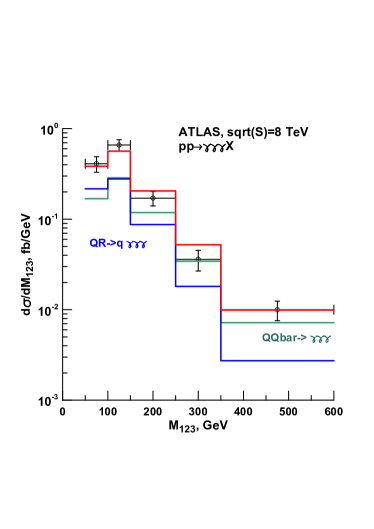
Figure 5: The differential cross sections for the production of three isolated photons as functions of $M_{123}=M_{3\gamma}$. The hard scale in PRA calculations are taken as invariant mass of three-photon system, $\mu_{0}=M_{3\gamma}$. The green histogram corresponds LO contribution from $Q\bar{Q}\to\gamma\gamma\gamma$ subprocess. The blue histogram corresponds NLO contribution from $QR\to q\gamma\gamma\gamma$ subprocess. The red histogram is their sum..

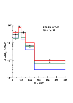
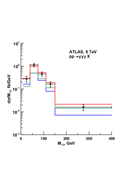
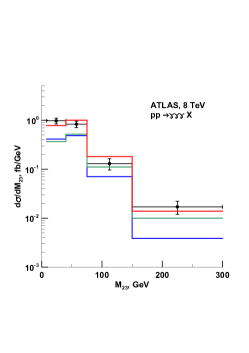
Figure 6: The differential cross sections for the production of three isolated photons as functions of $M_{12}$ (left panel), $M_{13}$ (central panel), $M_{23}$ (right panel). Curves are defined as in Fig. 5 .

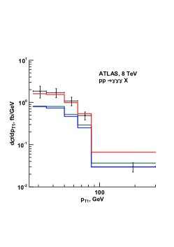
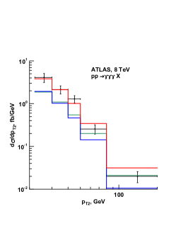
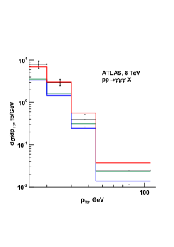
Figure 7: The differential cross sections for the production of three isolated photons as functions of $p_{T1}$ (left panel), $p_{T2}$ (central panel) and $p_{T3}$ (right panel). Curves are defined as in Fig. 5 .

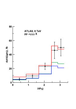
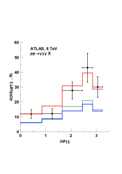
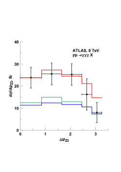
Figure 8: The differential cross sections for the production of three isolated photons as functions of $|\Delta\phi_{12}|$ (left panel), $|\Delta\phi_{13}|$ (central panel) and $\Delta\phi_{23}$ (right panel). Curves are defined as in Fig. 5 .

Figure 9: The differential cross sections for the production of three isolated photons as functions of $|\Delta\eta_{12}|$ (upper left panel), $|\Delta\eta_{13}|$ (upper right panel) and $|\Delta\eta_{23}|$ (bottom panel). Curves are defined as in Fig. 5 .

References

- (1) T. Aaltonen et al. [CDF], “Measurement of the Cross Section for Prompt Isolated Diphoton Production in Collisions at TeV,” Phys. Rev. D 84 (2011), 052006 doi:10.1103/PhysRevD.84.052006 [arXiv:1106.5131 [hep-ex]].
- (2) T. Aaltonen et al. [CDF], “Measurement of the Cross Section for Prompt Isolated Diphoton Production Using the Full CDF Run II Data Sample,” Phys. Rev. Lett. 110 (2013) no.10, 101801 doi:10.1103/PhysRevLett.110.101801 [arXiv:1212.4204 [hep-ex]].
- (3) G. Aad et al. [ATLAS], “Measurement of isolated-photon pair production in collisions at TeV with the ATLAS detector,” JHEP 01 (2013), 086 doi:10.1007/JHEP01(2013)086.
- (4) S. Chatrchyan et al. [CMS], “Measurement of differential cross sections for the production of a pair of isolated photons in pp collisions at ,” Eur. Phys. J. C 74 (2014) no.11, 3129 doi:10.1140/epjc/s10052-014-3129-3.
- (5) M. Aaboud et al. [ATLAS], “Measurement of the production cross section of three isolated photons in collisions at = 8 TeV using the ATLAS detector,” Phys. Lett. B 781 (2018), 55-76 doi:10.1016/j.physletb.2018.03.057
- (6) T. Binoth, J. P. Guillet, E. Pilon and M. Werlen, “A Full next-to-leading order study of direct photon pair production in hadronic collisions,” Eur. Phys. J. C 16 (2000), 311-330 doi:10.1007/s100520050024.
- (7) J. M. Campbell and C. Williams, “Triphoton production at hadron colliders,” Phys. Rev. D 89 (2014) no.11, 113001 doi:10.1103/PhysRevD.89.113001.
- (8) J. Alwall, et al., The automated computation of tree-level and next-to-leading order differential cross sections, and their matching to parton shower simula-tions, J. High Energy Phys. 07 (2014) 079, arXiv:1405.0301[hep -ph].
- (9) S. Catani, L. Cieri, D. de Florian, G. Ferrera and M. Grazzini, “Diphoton production at hadron colliders: a fully-differential QCD calculation at NNLO,” Phys. Rev. Lett. 108 (2012), 072001 [erratum: Phys. Rev. Lett. 117 (2016) no.8, 089901] doi:10.1103/PhysRevLett.108.072001.
- (10) J. M. Campbell, R. K. Ellis, Y. Li and C. Williams, “Predictions for diphoton production at the LHC through NNLO in QCD,” JHEP 07 (2016), 148 doi:10.1007/JHEP07(2016)148.
- (11) H. A. Chawdhry, M. L. Czakon, A. Mitov and R. Poncelet, “NNLO QCD corrections to three-photon production at the LHC,” JHEP 02 (2020), 057 doi:10.1007/JHEP02(2020)057
- (12) S. Kallweit, V. Sotnikov and M. Wiesemann, “Triphoton production at hadron colliders in NNLO QCD,” Phys. Lett. B 812 (2021), 136013 doi:10.1016/j.physletb.2020.136013 [arXiv:2010.04681 [hep-ph]].
- (13) J. Collins, “Foundations of perturbative QCD,” Camb. Monogr. Part. Phys. Nucl. Phys. Cosmol. 32, 1-624 (2011)
- (14) L. N. Lipatov, ”Reggeization Of The Vector Meson And The Vacuum Singularity In Nonabelian Gauge Theories”, Yad. Fiz. 23, 642 (1976) [Sov. J. Nucl. Phys. 23, 338 (1976)].
- (15) E. A. Kuraev, L. N. Lipatov, and V. S. Fadin, ”Multi - Reggeon Processes In The Yang-Mills Theory”, Zh. Eksp. Teor. Fiz. 71, 840 (1976) [Sov. Phys. JETP 44, 443 (1976)].
- (16) E. A. Kuraev, L. N. Lipatov and V. S. Fadin, ” The Pomeranchuk Singularity In Nonabelian Gauge Theories”, Zh. Eksp. Teor. Fiz. 72, 377 (1977) [Sov. Phys. JETP 45, 199 (1977)].
- (17) I. I. Balitsky and L. N. Lipatov, ” The Pomeranchuk Singularity In Quantum Chromodynamics”, Yad. Fiz. 28, 1597 (1978) [Sov. J. Nucl. Phys. 28, 822 (1978)];
- (18) B. A. Kniehl, V. A. Saleev, A. V. Shipilova and E. V. Yatsenko, “Single jet and prompt-photon inclusive production with multi-Regge kinematics: From Tevatron to LHC,” Phys. Rev. D 84 (2011), 074017 doi:10.1103/PhysRevD.84.074017 [arXiv:1107.1462 [hep-ph]].
- (19) M. Nefedov and V. Saleev, “Diphoton production at the Tevatron and the LHC in the NLO approximation of the parton Reggeization approach,” Phys. Rev. D 92, no. 9, 094033 (2015) doi:10.1103/PhysRevD.92.094033 [arXiv:1505.01718 [hep-ph]].
- (20) A. Karpishkov, V. Saleev and A. Shipilova, “Angular decorrelations in events at high energies in the parton Reggeization approach,” Mod. Phys. Lett. A 34 (2019) no.32, 1950266 doi:10.1142/S0217732319502663 [arXiv:1811.06942 [hep-ph]].
- (21) V. Saleev, “Production of three isolated photons in the high-energy factorization approach,” [arXiv:2107.11147 [hep-ph]].
- (22) R. K. Valeshabadi, M. Modarres and S. Rezaie, “Three-photon productions within the -factorization at the LHC,” Eur. Phys. J. C 81 (2021) no.11, 961 doi:10.1140/epjc/s10052-021-09771-9 [arXiv:2107.14607 [hep-ph]].
- (23) M. A. Kimber, A. D. Martin and M. G. Ryskin, “Unintegrated parton distributions,” Phys. Rev. D 63, 114027 (2001) doi:10.1103/PhysRevD.63.114027 [hep-ph/0101348].
- (24) G. Watt, A. D. Martin and M. G. Ryskin, “Unintegrated parton distributions and inclusive jet production at HERA,” Eur. Phys. J. C 31 (2003), 73-89 doi:10.1140/epjc/s2003-01320-4 [arXiv:hep-ph/0306169 [hep-ph]].
- (25) F. Hautmann, H. Jung, A. Lelek, V. Radescu and R. Zlebcik, “Collinear and TMD Quark and Gluon Densities from Parton Branching Solution of QCD Evolution Equations,” JHEP 01 (2018), 070 doi:10.1007/JHEP01(2018)070 [arXiv:1708.03279 [hep-ph]].
- (26) A. Bermudez Martinez, P. Connor, H. Jung, A. Lelek, R. Žlebčík, F. Hautmann and V. Radescu, Phys. Rev. D 99 (2019) no.7, 074008 doi:10.1103/PhysRevD.99.074008 [arXiv:1804.11152 [hep-ph]].
- (27) J. C. Collins and R. K. Ellis, “Heavy quark production in very high-energy hadron collisions,” Nucl. Phys. B 360 (1991), 3-30 doi:10.1016/0550-3213(91)90288-9
- (28) S. Catani and F. Hautmann, “High-energy factorization and small x deep inelastic scattering beyond leading order,” Nucl. Phys. B 427 (1994), 475-524 doi:10.1016/0550-3213(94)90636-X
- (29) M. A. Nefedov and V. A. Saleev, “High-Energy Factorization for Drell-Yan process in and collisions with new Unintegrated PDFs,” Phys. Rev. D 102 (2020), 114018 doi:10.1103/PhysRevD.102.114018 [arXiv:2009.13188 [hep-ph]].
- (30) L. N. Lipatov, “Gauge invariant effective action for high-energy processes in QCD,” Nucl. Phys. B 452, 369 (1995) doi:10.1016/0550-3213(95)00390-E [hep-ph/9502308].
- (31) L. N. Lipatov and M. I. Vyazovsky, “QuasimultiRegge processes with a quark exchange in the t channel,” Nucl. Phys. B 597, 399 (2001) doi:10.1016/S0550-3213(00)00709-4 [hep-ph/0009340].
- (32) M. A. Nefedov, V. A. Saleev and A. V. Shipilova, “Dijet azimuthal decorrelations at the LHC in the parton Reggeization approach,” Phys. Rev. D 87 (2013) no.9, 094030 doi:10.1103/PhysRevD.87.094030 [arXiv:1304.3549 [hep-ph]].
- (33) A. V. Karpishkov, M. A. Nefedov and V. A. Saleev, “ angular correlations at the LHC in parton Reggeization approach merged with higher-order matrix elements,” Phys. Rev. D 96 (2017) no.9, 096019 doi:10.1103/PhysRevD.96.096019 [arXiv:1707.04068 [hep-ph]].
- (34) M. Nefedov and V. Saleev, “On the one-loop calculations with Reggeized quarks,” Mod. Phys. Lett. A 32 (2017) no.40, 1750207 doi:10.1142/S0217732317502078 [arXiv:1709.06246 [hep-th]].
- (35) M. A. Nefedov, “Towards stability of NLO corrections in High-Energy Factorization via Modified Multi-Regge Kinematics approximation,” JHEP 08 (2020), 055 doi:10.1007/JHEP08(2020)055 [arXiv:2003.02194 [hep-ph]].
- (36) M. A. Nefedov, “Computing one-loop corrections to effective vertices with two scales in the EFT for Multi-Regge processes in QCD,” Nucl. Phys. B 946 (2019), 114715 doi:10.1016/j.nuclphysb.2019.114715 [arXiv:1902.11030 [hep-ph]].
- (37) E. N. Antonov, L. N. Lipatov, E. A. Kuraev and I. O. Cherednikov, “Feynman rules for effective Regge action,” Nucl. Phys. B 721 (2005), 111-135 doi:10.1016/j.nuclphysb.2005.013 [arXiv:hep-ph/0411185 [hep-ph]].
- (38) A. Karpishkov, V. Saleev and A. Shipilova, “Large- production of D mesons at the LHCb in the parton Reggeization approach,” [erratum: Phys. Rev. D 94 (2016) no.11, 114012] doi:10.1103/PhysRevD.94.114012 [arXiv:1610.04975 [hep-ph]].
- (39) R. Maciuła, V. A. Saleev, A. V. Shipilova and A. Szczurek, “New mechanisms for double charmed meson production at the LHCb,” Phys. Lett. B 758 (2016), 458-464 doi:10.1016/j.physletb.2016.05.052 [arXiv:1601.06981 [hep-ph]].
- (40) A. V. Karpishkov, M. A. Nefedov, V. A. Saleev and A. V. Shipilova, “B-meson production in the Parton Reggeization Approach at Tevatron and the LHC,” Int. J. Mod. Phys. A 30 (2015) no.04n05, 1550023 doi:10.1142/S0217751X15500232 [arXiv:1411.7672 [hep-ph]].
- (41) V. A. Saleev, M. A. Nefedov and A. V. Shipilova, “Prompt J/psi production in the Regge limit of QCD: From Tevatron to LHC,” Phys. Rev. D 85 (2012), 074013 doi:10.1103/PhysRevD.85.074013 [arXiv:1201.3464 [hep-ph]].
- (42) Z. G. He, B. A. Kniehl, M. A. Nefedov and V. A. Saleev, “Double Prompt Hadroproduction in the Parton Reggeization Approach with High-Energy Resummation,” Phys. Rev. Lett. 123 (2019) no.16, 162002 doi:10.1103/PhysRevLett.123.162002 [arXiv:1906.08979 [hep-ph]].
- (43) See Supplemental Material at http://link.aps.org/ supplemental/10.1103/PhysRevD.92.094033 to obtain the ReggeQCD model file.
- (44) T. Hahn, “Generating Feynman diagrams and amplitudes with FeynArts 3,” Comput. Phys. Commun. 140 (2001), 418-431 doi:10.1016/S0010-4655(01)00290-9 [arXiv:hep-ph/0012260 [hep-ph]].
- (45) A. van Hameren, “KaTie : For parton-level event generation with -dependent initial states,” Comput. Phys. Commun. 224 (2018), 371-380 doi:10.1016/j.cpc.2017.11.005 [arXiv:1611.00680 [hep-ph]].
- (46) A. van Hameren, P. Kotko and K. Kutak, “Helicity amplitudes for high-energy scattering,” JHEP 01 (2013), 078 doi:10.1007/JHEP01(2013)078 [arXiv:1211.0961 [hep-ph]].
- (47) A. van Hameren, K. Kutak and T. Salwa, “Scattering amplitudes with off-shell quarks,” Phys. Lett. B 727 (2013), 226-233 doi:10.1016/j.physletb.2013.10.039 [arXiv:1308.2861 [hep-ph]].
- (48) K. Kutak, R. Maciula, M. Serino, A. Szczurek and A. van Hameren, “Four-jet production in single- and double-parton scattering within high-energy factorization,” JHEP 04 (2016), 175 doi:10.1007/JHEP04(2016)175 [arXiv:1602.06814 [hep-ph]].
- (49) S. Frixione, “Isolated photons in perturbative QCD,” Phys. Lett. B 429 (1998), 369-374 doi:10.1016/S0370-2693(98)00454-7 [arXiv:hep-ph/9801442 [hep-ph]].