Theory of the Energy Variance in a Quantum Bit

Abstract

The energy of a driven two-level quantum system —or quantum bit (qubit)— can be exactly (i.e. without the use of the rotating wave approximation) defined by the time derivatives of its large-amplitude, high-frequency internal as well as overall phases. We show that their envelope can be derived from the quantum expectation value $\langle\mathbf{V}\rangle=\langle\Psi|\mathbf{V}|\Psi\rangle$ of the time-dependent Hermitian variance operator $\mathbf{V}=[\mathbf{H}-\langle\mathbf{H}\rangle\mathbf{I}]^{2}$. Indeed, following standard statistical physics, we formally define this latter by the use of the Hamiltonian $\mathbf{H}$, the state $\Psi$ and the energy mean value $\langle\mathbf{H}\rangle=\langle{\Psi}|\mathbf{H}|{\Psi}\rangle$ of the system ($\mathbf{I}$ being the identity matrix). Remarkably, the resulting standard deviation $\sigma=\sqrt{\langle\mathbf{V}\rangle}$ may become comparable to the energy mean value itself. We have indeed $\sigma\sim\langle\mathbf{H}\rangle$ in the case of a weak Rabi drive. Therefore $\sigma$ yields a large statistical time-dependent range of available values for the qubit energy about its well-known harmonic Rabi state flipping $\langle\mathbf{H}\rangle$. By which experimental protocol can such a intriguing quantum property be verified? In the spirit of a recent comment (I. Mazin, Nature Physics 2022, 18, 367), we point out the experimental measurement of the so-called “time-of-flight” values of an abrupt quantum jump (Z. Minev et al. Nature 2019, 570, 200) as a possible candidate for such a protocol. We show that we quite simply recover these abrupt quantum jumps by use of both the present theory and the quantum Zeno effect.

.1 Introduction

How can the energy variance of a two-state quantum system —conservative or not— be defined and what is the physical meaning of its corresponding standard deviation? To answer these questions, the present paper proposes a rigourous —no rotating wave approximation (RWA)— quantum theory that formally duplicates the standard definition of variance in statistical physics. It shows through the discussion of a recent experiment Minev et al. (2019) how such a theoretical background can actually apply.

Adopting the bra-ket formalism, one first recalls the standard quantum expectation –or “average”, or “mean”– value:

$$\langle\mathbf{H}\rangle=\langle{\Psi}|\mathbf{H}|{\Psi}\rangle$$ (1)

of the energy by use of the Hamitonian $\mathbf{H}$ of the system and its wavefunction $\Psi$. Then, one might wish to introduce the following variance operator ($\mathbf{I}$ is the identity matrix):

$$\mathbf{V}=[\mathbf{H}-\langle\mathbf{H}\rangle\mathbf{I}]^{2},$$ (2)

that is directly extrapolated from standard statistical physics. This operator is Hermitian with two real eigenvalues. The resulting variance expectation value:

$$\langle\mathbf{V}\rangle=\langle{\Psi}|\mathbf{V}|{\Psi}\rangle,$$ (3)

yields the corresponding standard deviation:

$$\mathbf{\sigma}=\sqrt{\langle\mathbf{V}\rangle}$$ (4)

of the energy with respect to its mean-value (1). How can such a formal dispersion of energy values about $\langle\mathbf{H}\rangle$ be measured?

In order to answer this basic question, we refer to the exact solution of the Hamiltonian equations of motion of a driven qubit Reinisch (1998a) Reinisch (1998b). Since the RWA is discarded, one keeps the two high-frequency energy components $E_{a,b}(t)$ related to the qubit’s energy mean value (1) by:

$$\langle\mathbf{H(t)}\rangle=|\psi_{a}(t)|^{2}E_{a}(t)+|\psi_{b}(t)|^{2}E_{b}(t).$$ (5)

Here the so-called “state energies” $E_{a,b}(t)$ are defined in the next section by the time derivatives of the qubit’s internal and overall phases while $\psi_{a,b}(t)$ are the spinor components of its wavefunction $\Psi(t)$. We assume that its Hamiltonian $\mathbf{H(t)}$ is defined by the external time-dependent energy drive ${\cal E}(t)$ and by the off-diagonal constant $K$ through the two Pauli matrices as:

$${\Psi}(t)=\begin{pmatrix}\psi_{a}(t)\\ \psi_{b}(t)\end{pmatrix}\quad;\quad\mathbf{H}(t)=\begin{pmatrix}{\cal E}(t)&{K}\\ {K}&-{\cal E}(t)\end{pmatrix}.$$ (6)

We show that the envelope of the state energies $E_{a,b}(t)$ is quite accurately determined by the quantum standard deviation (4). Since they are simply phase-shifted by $\pi$ Reinisch (1998a), they are almost redundant. Therefore their mean value within their high-frequency period $T$ is equal to $\langle\mathbf{H}\rangle$ as shown by eq. (5) Reinisch (1998a). This explains the role played by $\mathbf{\sigma}$ in an energy measurement process. Indeed, if the measurement at time $t$ lasts less than $T$, it yields either of the two state energies $E_{a,b}(t)$. Conversely, if it lasts more than $T$, it yields $\langle\mathbf{H}\rangle$ and no special effect due to $\mathbf{\sigma}$ can be observed. Therefore the standard deviation (4) will play a leading role in any series of energy measurements whose frequency is higher than $1/T$. The quantum Zeno effect (QZE) hence appears as the ideal candidate for an experimental check of the present theory because it demands frequent (almost continuous) measurements Itano (2019). Then QZE inhibits the decay of an unstable quantum system through the wave-function collapse described by the quantum measurement theory Von Neumann (1932): the system evolves from the same initial state after every measurement B. Misra and Sudarshan (1977)D. Home and Whitaker (1993).

This effect has been beautifully verified by use of a Rabi-driven two-level quantum system Itano et al. (1990) —namely, a ground state —G¿ and an excited state —D¿— with the addition of a 3rd “ancilla” state —B¿ that actually plays the role of the continuously-operating ground-state population measurement Cook (1988). Specifically, state —B¿ is connected by a strongly allowed transition to level —G¿ and it can decay only to —G¿. The continuous state measurement is carried out by resonantly (Rabi) driving the $G\rightarrow B$ transition with an appropriately designed optical pulse. This measurement causes a collapse of the wave function as told above. If the system is projected into the ground-state level —G¿ at the beginning of the pulse, it cycles between —G¿ and —B¿ and emits a series of photons —hence the label —B¿ for “bright”— until the pulse is turned off. If it is projected into the excited level —D¿ (for “dark”), it scatters no photons. Therefore the wave-function collapse is due to a null measurement Porrati and Putterman (1987) Raimond (2020). That is, the absence of scattered photons when the optical pulse is applied is enough to cause a collapse of the wave function to level —D¿ Itano et al. (1990).

A recent outstanding experiment has reproduced this experimental set-up Minev et al. (2019). It led to the occurence of sudden, quite abrupt quantum jumps. The agreement between the observation and the theoretical predictions —based on the arduous modern quantum trajectory theory Minev (2018)— is excellent. In order to put to the test the present theory, we wish to recover the existence of these abrupt quantum jumps by a quite simple alternative explanation derived from the above quantum-variance properties. We believe that this scope is in agreement with the spirit stressed in Mazin (2022).

.2 Theory

In the normalized two-state $|a,b\rangle$ base, the Schrödinger equation:

$$i\hbar\frac{\mathrm{d}}{\mathrm{d}t}{\Psi}=\mathbf{H}{\Psi}$$ (7)

defined by Eqs (6) is equivalent to the following Hamiltonian formulation of classical-like mechanics by use of the two conjugate canonical coordinates $\delta(t)$ and $\alpha(t)$:

$$\dot{\alpha}=-\frac{\partial{\cal H}}{\partial\delta}=\sqrt{1-\alpha^{2}}\sin\delta\quad;\quad\dot{\delta}=\frac{\partial{\cal H}}{\partial\alpha}=-\frac{\alpha}{\sqrt{1-\alpha^{2}}}\cos\delta+{\cal E}(\tau),$$ (8)

whose Hamiltonian is:

$${\cal H}=\sqrt{1-\alpha^{2}}\cos\delta+\alpha{\cal E}(\tau),$$ (9)

provided Reinisch (1998a) Reinisch (1998b):

$$\psi_{a}(t)=\sqrt{\frac{1+\alpha(t)}{2}}e^{i\Theta(t)}\quad;\quad\psi_{b}(t)=\sqrt{\frac{1-\alpha(t)}{2}}e^{i[\Theta(t)+\delta(t)]}.$$ (10)

In the above (8-9) Hamiltonian dynamical system (or HDS), the dot means the derivation with respect to the dimensionless time $\tau=\Omega t$ with $\Omega=2{K}/\hbar$ (e.g. it is the Larmor frequency of a two-level spin one-half system). Hence we assume in the present work:

$${K}=1\quad;\quad\hbar=2\quad;\quad\Omega=1.$$ (11)

The angular positions $\theta$ and $\phi$ on the qubit’s Bloch sphere are straightforward:

$$\alpha=\cos\theta\quad;\quad\phi=\Theta+\frac{\delta}{2}.$$ (12)

Then:

$$\psi_{a}(t)=e^{i\phi(t)}\cos\frac{\theta(t)}{2}e^{-i\delta(t)/2}\quad;\quad\psi_{b}(t)=e^{i\phi(t)}\sin\frac{\theta(t)}{2}e^{+i\delta(t)/2}.$$ (13)

Note that the time-dependent overall phase $\Theta(\tau)$ in (10) is not a 3rd independent variable: it is slaved to the solution of HDS (8-9) by:

$$\dot{\Theta}=-\frac{1}{2}\Bigl{[}\sqrt{\frac{1-\alpha}{1+\alpha}}\cos\delta+{\cal E}(\tau)\Bigr{]}.$$ (14)

Contrary to intuitive opinions, the dynamics of the overall phase of a quantum state can indeed yield an observable physical effect (e.g. it causes the famous $4\pi$-symmetry of spinor wave functions that have been directly verified in both division-of-amplitude H. Rauch et al. (1975)Werner et al. (1975) and division-of-wave-front Klein and Opat (1976) neutron interferometry experiments). When $\alpha\equiv 0$ (which is Feynman’s rough assumption in his textbook description of the stationary Josephson effect Feynman et al. (1965) ), Eqs. (8) yield the two Josephson equations (${\cal E}$ is then the applied voltage).

In the simplest conservative case ${\cal E}\equiv 0$, the classical-like HDS orbits defined by Hamilton equations (8) do all have the same reduced frequency +1 (actually $+\Omega$) for ${\cal H}>0$ (resp. -1, or $-\Omega$, for ${\cal H}<0$). They define the corresponding quantum superposition states of the system in agreement with Eqs. (10) and (14) Reinisch (1998a). Such a binary structure of the orbit frequency, namely $\pm\Omega$ in actual units, is the translation in terms of the HDS equations of motion (8-9) and action Reinisch (2021), of the eigenvalues $\pm 1$ in the two-level energy spectrum of the undriven qubit. In the driven, however still conservative case ${\cal E}\equiv constant\neq 0$, all the orbits do still keep the same angular frequency $\pm\sqrt{1+{\cal E}^{2}}$ (i.e. the corresponding eigenvalues), depending on the sign of ${\cal H}$. Moreover it has also been shown in Reinisch (1998a) that the above-mentioned $4\pi$ symmetry of the overall qubit phase $\Theta$ becomes an immediate consequence of the HDS solution of Eq.  (14).

We have in accordance with Eqs. (1), (6), (9) and (10) the following fundamental link between the mean qubit energy $\langle\mathbf{H}\rangle$ and the HDS energy ${\cal H}$ in the dimensionless units (11):

$$\langle\mathbf{H}(\tau)\rangle={\cal H}(\tau).$$ (15)

Equations (5-10) and (15) yield the following HDS definition of the two qubit’s time-dependent state energies in the dimensionless units (11):

$$E_{a}=\frac{{\cal H}+{\cal E}}{1+\alpha}\quad;\quad E_{b}=\frac{{\cal H}-{\cal E}}{1-\alpha}.$$ (16)

They are the derivatives of the two internal as well as overall phases $\delta(\tau)$ and $\Theta(\tau)$:

$$E_{a}=-\hbar\frac{\mathrm{d}\Theta}{\mathrm{d}t}=-2{\dot{\Theta}}\quad;\quad E_{b}=-\hbar\frac{\mathrm{d}(\Theta+\delta)}{\mathrm{d}t}=-2(\dot{\Theta}+\dot{\delta}),$$ (17)

by use of Eqs. (8) and (14). They provide an explicit fine-structure mapping of the dynamical properties of the classical-like HDS trajectories (8-9) onto the mean quantum energy (5) and onto its state energy variance:

$$\sigma_{a,b}^{2}(\tau)=|\psi_{a,b}(\tau)|^{2}[E_{a,b}(\tau)-{\cal H}(\tau)]^{2},$$ (18)

in terms of the standard deviations $\pm\sigma_{a,b}(\tau)$. The necessary link with the quantum variance (2-3) is performed as follows. Using (15), we have:

$$\mathbf{V}=\begin{pmatrix}({\cal H}-{\cal E})^{2}+K^{2}&-2K{H}\\ -2K{H}&({\cal H}+{\cal E})^{2}+K^{2}\end{pmatrix},$$ (19)

and therefore, by use of Eqs. (3) and (10):

$$\langle\mathbf{V}\rangle=(1-2K){\cal H}^{2}+2(K-1)\alpha{\cal E}{\cal H}+{\cal E}^{2}+K^{2}.$$ (20)

Since we assume $K=1$ in accordance with (11), Eq. (20) becomes:

$$\langle\mathbf{V}\rangle={\cal E}^{2}-{\cal H}^{2}+1\sim 1-{\cal H}^{2},$$ (21)

if the qubit is weakly Rabi-driven as envisaged in the next section. Then the link between the quantum-variance standard deviation (4) and the state-energy ones (18) becomes clear: see Fig. 1.

.3 Weak Rabi drive

When the weak resonant field:

$${\cal E}(\tau)=A\sin\tau\quad;\quad A\ll 1,$$ (22)

is applied to the system, we obtain in accordance with Eq. (9) the well-known quasi-harmonic Rabi oscillation between the two eigenvalues $\pm 1$ of the mean energy:

$${\cal H}\sim\cos\frac{A\tau}{2}+\Delta{\cal H}\quad;\quad\Delta{\cal H}=\alpha{\cal E}(\tau)=A\alpha\sin\tau\ll 1.$$ (23)

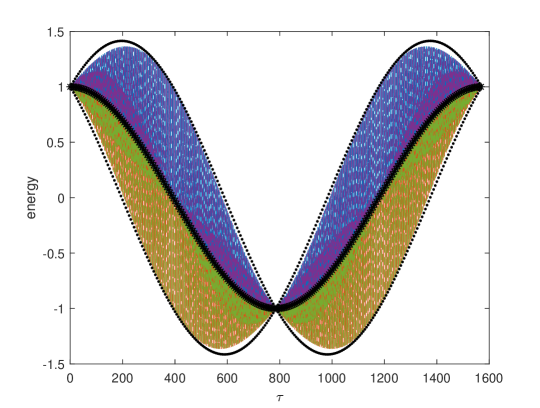
Figure 1: Validation of the state-energy description (16-18) by use of the variance Hermitian operator (2-3) for $A=8\,10^{-3}$. The qubit’s colored energy regions are defined by the state-energy standard deviation dressing (18) of Rabi’s quasi-harmonic HDS Hamiltonian —or mean energy— (23) during one Rabi period $4\pi/A=1571$ in reduced units (11) (thick black plot). Dotted black plot: the quantum standard deviations (4) about ${\cal H}$ as defined by quantum variance (21).

One obtains a regime of HDS quasiperiodic orbits slowly spiraling out of one ${\cal H}=\pm 1$ eigenvalue cell og in to the next ${\cal H}=\mp 1$ one Reinisch (1998b). The corresponding “dressing” of the quasi-harmonic mean energy value (23) by the state-energy standard deviations defined by variance (18) is quite spectacular Reinisch (2021). In Fig. 1, ${\cal H}(\tau)$ is displayed by the thick black plot while the quantum standard deviations about it, defined by Eq. (4) and by quantum variance (20), are shown by the dotted black plots. The quite dense colored patterns enclosed by these latter are built from the very-high-frequency oscillatory standard deviations (18) with extremely small HDS orbit period $\sim 2\pi\ll 1571$ at the scale of the Rabi period $4\pi/A=1571$. The standard deviations $+\sigma_{a}(\tau)$ (continuous purple) and $-\sigma_{a}(\tau)$ (continuous green) due to state energy $E_{a}(\tau)$ defined in (16) are phase-shifted by $\sim\pi$ with respect to the standard deviations $+\sigma_{b}(\tau)$ (dotted purple) and $-\sigma_{b}(\tau)$ (dotted green) due to state energy $E_{b}(\tau)$. All these very-high-frequency standard deviations display the rather important dispersion of the qubit energy about its mean value ${\cal H}$ except at the two eigenvalues $\pm 1$ where, as expected, this dispersion vanishes. We note with interest that these standard deviation patterns are quite accurately bounded by the quantum standard deviations (4) defined by the quantum variance (20). This remarkable property establishes the statistical link between the variance Hermitian operator description (2-3) and the state-energy one (16-18). It validates the self-consistency of the present theory.

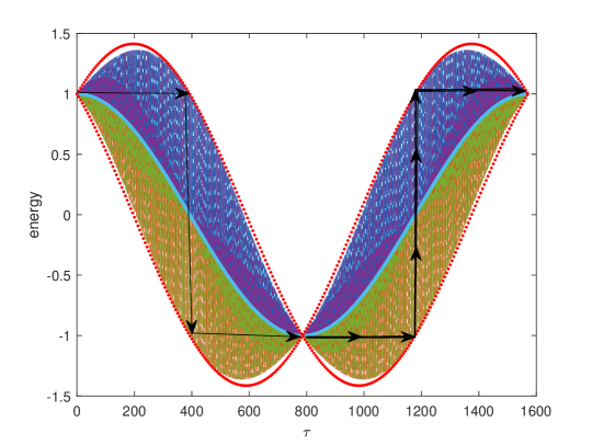
Figure 2: $A=8\,10^{-3}$: the qubit energy regions defined by Fig. 1 together with the quasi-harmonic HDS Hamiltonian ${\cal H}$ (in continuous blue) and the quantum standard deviations defined by Eqs   (4) and (20) about ${\cal H}$ (red dotted plots). The general principle of a step-like quantum jump due to the series of repetitive eigenstate measurements is illustrated by arrows. The thick arrows display the abrupt energy jump occuring at $\tau=1183$ (actually at ${\cal H}=0$) from the ground state $E=-1$ to the excited level $E=+1$. The thiner path displays the reverse de-excitation process.

.4 Quantum Zeno jump

The measured “’time-of-flight” values obtained by a continuous measurement process in experiment Minev et al. (2019) have been recovered in the frame of the above theory by considering the quantization of the HDS action Reinisch (2021). Here we wish to show in addition that these values are actually an immediate first-principle consequence of Fig. 1 and —contrary to the quantum trajectory description given in Minev et al. (2019)— they do not depend on the specific continuous measurement process (provided this latter is long-lasting enough). Indeed any such process yields QZE “freezing” of the corresponding quantum states in their initial configuration Itano (2019) B. Misra and Sudarshan (1977) and this freezing remains possible as long as the resulting trajectory lies inside of the qubit’s energy region defined by Fig. 1.

Let us be specific and consider Fig. 2. Assume that the system, while still resonantly Rabi-driven by (22), is initially in, say, its ground state $-1$ (i.e. at half the Rabi period $\tau=785$) and introduce a repetitive measurement process in accordance with Itano et al. (1990) or, equivalently, with Minev et al. (2019) (the following applies as well when we start from the excited state: see Fig. 2 at $\tau=0$). Then, due to QZE which acts as a strong perturbation, the system is forced to remain “frozen” in this lowest energy value instead of starting Rabi’s harmonic excitation dynamics (23) (displayed by the blue line). Consequently, its energy keeps its value $-1$ along the horizontal segment as $\tau$ increases for $785<\tau<1183$ (lowest horizontal arrow path), i.e. as long as the energy of the system stays within the statistically accessible energy region about ${\cal H}$ that is defined by Eq. (18), or equivalently by Eqs (4) and (20) (dotted red line). When reaching this boundary at $\tau=1183$, it jumps to the excited level $+1$ in accordance with the vertical arrow path in order to continue the QZE state freezing process from $\tau=1183$ to $\tau=1571$ if the repetitive measurement is lasting over a time interval greater than this half Rabi period. This QZE jump —which we call “quantum Zeno jump” (QZJ)— actually absorbs at once all the energy input due to the external Rabi drive that has been stored in the system during its forced QZE freezing stage in its ground state.

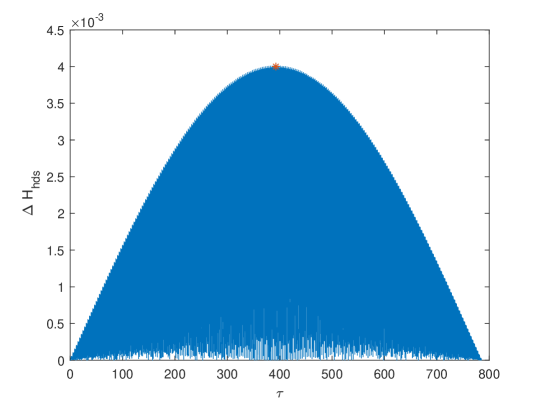
Figure 3: The quasi-stochastic energy input $\Delta{\cal H}$ defined by Eq. (23) over half a Rabi period $2\pi/A$ when the origin of time is now taken at $\tau=785$ in Figs. 1-2. Its seemingly two-dimensional dense pattern results from its extremely fast oscillations at the scale of the Rabi period. Therefore it will be regarded as the uncertainty in the energy input at a given time $\tau$. The star indicates the maximum at $\tau=393$ or ${\cal H}=0$ that scales this uncertainty in (24).

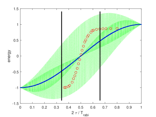
Figure 4: Second (r.h.s.) part of Figs. 1-2 illustrating the QZE-vs-Rabi excitation process of Fig. 2 by use of the data provided with Minev et al. (2019). Blue plot: Rabi’s mean energy defined by Eq. (23). Circles: the path in the Hilbert space followed by the jump evolutions given in Fig. 3b of Ref. Minev et al. (2019), using its $T_{Rabi}=50\,\mu$s Rabi period for the normalization of the $\tau$-axis. The $13\%$ deviation from the excited eigenvalue +1 is due to imperfections, mostly excitations to higher levels Minev et al. (2019). The two vertical bars display the minimum duration $\Delta\tau_{min}$ of the transition obtained as the consequence of the uncertainty principle (24) when the perturbation $\Delta{\cal H}$ illustrated by Fig. 3 is maximum (star). These bars fit quite well with the duration of the so-called “time-of-flight” value $\sim 2\Delta_{mid}$ given in Minev et al. (2019). Therefore they experimentally validate the present generic theory.

The above QZJ scheme is oversimplified. Indeed the standard deviation boundary at $\tau=1183$ is only statistical: it has not a precise definite value. Therefore the QZJ may occur at any time in the interval $\Delta\tau$ about $\tau=1183$. When trying to evaluate it, one should regard the Hamiltonian driving term $\Delta{\cal H}$ in (23) as a quasi-stochastic energy input, as shown by Fig. 3. Indeed, $\Delta{\cal H}$ oscillates extremely rapidly at the scale of the Rabi period $4\pi/A$. It actually looks like a mere two-dimensional uniformly-dense drive pattern and thus yields the corresponding time interval $\Delta\tau$:

$$\Delta{\cal H}\Delta\tau\geq\frac{\hbar}{2}=1,$$ (24)

(cf. our choice (11) of the reduced units) in which any step-like QZJ illustrated by Fig. 2 can statistically occur. Since the QZJ formely appears at half the gap defined by ${\cal H}=0$ (cf. Fig. 2), we take $\Delta{\cal H}=\Delta{\cal H}_{max}=4\,10^{-3}$ in (24) —see the star in Fig. 3— and therefore $\Delta\tau_{min}\sim 1/\Delta{\cal H}_{max}\sim 250$. This time interval is pictured by the two vertical bars in Fig. 4 where the experimental data given in Fig. 3b of Ref. Minev et al. (2019) are reproduced by use of red circles, using for the normalization of our $\tau$-axis the experimental Rabi period $T_{Rabi}=50\,\mu s$ given in Minev et al. (2019) (their $\sim 13\%$ deviation from the excited eigenvalue +1 is due, the authors say, to imperfections, mostly excitations to higher levels). We see that $\Delta\tau_{min}\sim 250\sim\sim 2\Delta_{mid}$ agrees fairly well with the so-called “time-of-flight” value $\sim 2\Delta_{mid}$ given in Fig. 3b of Minev et al. (2019). Moreover, $\Delta\tau_{min}$ is also in good agreement with HDS action quantization when the system crosses the separatrix of the system at ${\cal H}=0$ Reinisch (2021). Recall that Heisenberg’s l.h.s. of inequality (24) has indeed the dimension of an action.

.5 Conclusion

The present work defines a new quantum Hermitian operator —the energy variance operator $\mathbf{V}$— which is simply duplicated from the statistical definition of energy variance in classical physics. Its expectation value yields the standard deviation $\sigma$ of the energy about its mean value $\langle\mathbf{H}\rangle$. We show by use of an exact Hamiltonian description that $\sigma$ is actually due to the very-high-frequeny energy oscillations about $\langle\mathbf{H}\rangle$ which are usually discarded in the rotating wave aproximation (RWA). Therefore the present theory restores the fundamental physical interest of these latter: while the RWA yields quite accurately the Rabi oscillations of $\langle\mathbf{H}\rangle$, the standard deviation $\sigma$ about $\langle\mathbf{H}\rangle$ is a mere signature of the existence of very-high-frequeny energy oscillations $E_{a,b}$ in the system. As a consequence, the experimental effect of $\sigma$ will be important only within their period while it will average to $\langle\mathbf{H}\rangle$ when the measurement process lasts more than such a period. In the present state of the art, the quantum Zeno effect (QZE) seems to be the ideal experimental candidate for the detection of $\sigma$ since it is due to a series of high-frequency measurements whose period may well become less than that of the energy oscillations $E_{a,b}$. This is indeed the case in the experimental measurements of the duration of quantum jumps Minev et al. (2019) since they were actually performed by reproduction of the original set-up that led to the experimental discovery of QZE Itano et al. (1990). The agreement of our results with those displayed in Minev et al. (2019) constitutes a clear evidence of the physical interest of the standard deviation, and hence of the variance operator $\mathbf{V}$, in the definition of the energy of the system.

Two final comments: - We considered a weak resonant Rabi drive in order to compare with the experimental results found in Minev et al. (2019). The case of a strong Rabi drive has been considered in Reinisch (2022). It was shown there that the definition of the state energies energies $E_{a,b}$ still remains valid. Their spectrum however may appear either chaotic or discrete (frequency combs) due to phase-locked cycles in the solution of the Hamiltonian differential system. - The present definition of the energy variance operator $\mathbf{V}$ may actually be generalized to any observable operator $\mathbf{O}$. Then its variance operator will simply be $\mathbf{V[O]=[O-\langle O\rangle I]^{2}}$ and its resulting expectation value $\langle\mathbf{V[O]}\rangle$ in a given state $\Psi$ will define the corresponding standard deviation about $\langle\mathbf{O}\rangle$ in any measurement process that takes into account the high-frequency components of the Schrödinger solution.

References

- Minev et al. (2019) Z. Minev, S. Mundhada, S. Shankar, P. Reinhold, R. Gutiérrez-Jáuregui, R. Schoelkopf, M. Mirrahimi, H. Carmichael, and M. Devoret, Nature 570, 200 (2019).
- Reinisch (1998a) G. Reinisch, Physica D 119, 239 (1998a).
- Reinisch (1998b) G. Reinisch, Phys. Lett. A 238, 107 (1998b).
- Itano (2019) W. Itano, Current Science 116, , 201 (2019).
- Von Neumann (1932) J. Von Neumann, Die mathematischen Grundlagen der Quantenmechanik (Springer Berlin, 1932).
- B. Misra and Sudarshan (1977) B. B. Misra and E. Sudarshan, J. Math. Phys. 18, 756 (1977).
- D. Home and Whitaker (1993) D. D. Home and M. Whitaker, Phys. Lett. A 173, 327 (1993).
- Itano et al. (1990) W. Itano, D. Heinzen, J. Bollinger, and D. . Wineland, Phys. Rev. A 41, 2295 (1990).
- Cook (1988) R. J. Cook, Phys. Scr. T21, 49 (1988).
- Porrati and Putterman (1987) M. Porrati and S. Putterman, Phys. Rev. A 36, 929 (1987).
- Raimond (2020) J. M. Raimond, La Recherche 555, 41 (2020).
- Minev (2018) Z. K. Minev, Ph.D. thesis, Yale university (2018).
- Mazin (2022) I. Mazin, Nature Physics 18, 367 (2022).
- H. Rauch et al. (1975) H. H. Rauch, A. Zeilinger, G. Badurek, A. Wilting, W. Bauspiess, and U. Bonse, Phys. Lett. A 54, 425 (1975).
- Werner et al. (1975) S. Werner, R. Colella, A. Overhauser, and C. Eagen, Phys. Rev. Lett. 35, 1053 (1975).
- Klein and Opat (1976) A. Klein and G. Opat, Phys. Rev. Lett. 37, 238 (1976).
- Feynman et al. (1965) R. Feynman, R. Leighton, and M. Sands, The Feynman Lectures on Physics (Addison-Wesley, 1965).
- Reinisch (2021) G. Reinisch, Results inPhysics 29, 104761 (2021), doi.org/10.1016/j.rinp.2021.104761.
- Reinisch (2022) G. Reinisch, Results Phys 33, 105136 (2022), doi.org/10.1016/j.rinp.2021.105136.