Deep Interpretable Ensembles

Abstract

Ensembles improve prediction performance and allow uncertainty quantification by aggregating predictions from multiple models. In deep ensembling, the individual models are usually black box neural networks, or recently, partially interpretable semi-structured deep transformation models. However, interpretability of the ensemble members is generally lost upon aggregation. This is a crucial drawback of deep ensembles in high-stake decision fields, in which interpretable models are desired. We propose a novel transformation ensemble which aggregates probabilistic predictions with the guarantee to preserve interpretability and yield uniformly better predictions than the ensemble members on average. Transformation ensembles are tailored towards interpretable deep transformation models but are applicable to a wider range of probabilistic neural networks. In experiments on several publicly available data sets, we demonstrate that transformation ensembles perform on par with classical deep ensembles in terms of prediction performance, discrimination, and calibration. In addition, we demonstrate how transformation ensembles quantify both aleatoric and epistemic uncertainty, and produce minimax optimal predictions under certain conditions.

1 Introduction

The need for interpretable yet flexible and well-performing prediction models is great in high-stakes decisions fields, such as medicine. Practitioners need to be able to understand how a model arrives at its predictions, and how confident these predictions are, to assess a model’s trustworthiness. For this purpose, Rudin (2019) proposes the use of intrinsically interpretable models. A model is deemed intrinsically interpretable, if it possesses a transparent structure, such as sparsity or additivity with parameters that can be interpreted, e.g., as log odds-ratios or log hazard-ratios. For instance, traditional statistical regression models, e.g., linear regression, or the Cox proportional hazards model (Cox, 1972), and also decision trees fall in this category. However, contemporary applications may involve more complex data or require methods, for which intrinsic interpretability can only partly be achieved. For models that are not intrinsically interpretable there exist post hoc or model-agnostic explanation methods (for an overview, see Molnar, 2020).

Nowadays the available data for prediction is often a mix of structured tabular and unstructured data, such as images, text, or speech. The prediction target can be continuous (e.g., time-to-event), or discrete (e.g., number of recurrences, or an ordinal score, such as tumour-grading). Hence, the ideal prediction model should in summary (i) be as interpretable as possible, (ii) yield accurate and calibrated probabilistic predictions, and (iii) be applicable to multi-modal input data and different kinds of outcomes. One group of models fulfilling these requirements are deep transformation models (Sick et al., 2021; Baumann et al., 2021; Kook et al., 2022; Rügamer et al., 2021). Deep transformation models estimate the conditional distribution of an outcome given all available data modalities. However, a single instance of such a model may suffer from overfitting and overconfident predictions, which may lead to severe prediction errors when applied to novel data.

To build well-performing models, it is common practice to aggregate the predictions of several models, mitigating overconfident and potentially inaccurate predictions (Bühlmann, 2012). Aggregating several models is referred to as ensembling, and the resulting final model is called an ensemble. Deep ensembling, i.e., aggregating predictions of (often as few as 3–5) deep neural network that are fitted on the same data but with different random initializations, has been demonstrated to notably improve prediction performance and uncertainty quantification (Lakshminarayanan et al., 2017). We refer to this approach as classical deep ensembling. However, classical deep ensembles are black boxes even if their members are somewhat interpretable individually.

In this paper, we propose transformation ensembles, which preserve structure and interpretability of their members. In addition, transformation ensembles improve predictions and allow uncertainty quantification with distributional deep neural networks.

1.1 Our contribution

We present transformation ensembles as a novel way to aggregate predicted cumulative distribution functions (CDFs) derived from deep neural networks with a special focus on deep transformation models for (potentially) semi-structured data. We show that transformation ensembles (i) preserve structure and interpretability of their members, (ii) improve the prediction performance akin to classical deep ensembles, and (iii) minimize worst-case prediction error in special cases. We showcase these properties theoretically and demonstrate the benefits of transformation ensembles empirically on several semi-structured data sets. With transformation ensembles we are able to provide empirical evidence for answering open questions in deep ensembling (Abe et al., 2022). For instance, the increased flexibility of classical deep ensembles over their members does not seem to be necessary for improving prediction performance or allowing uncertainty quantification.

Structure of this paper

We discuss how transformation ensembles relate to classical deep ensembles and other ensembling strategies from the forecasting literature in Section 1.2. We give the necessary background on scoring rules, ensembling and transformation models in Section 2. Afterwards, we present transformation ensembles (Section 3) and demonstrate how they improve prediction performance similar to deep ensembles while preserving interpretability (Section 5). We end with a discussion of our results and potential directions of future research (Section 6). Mathematical notation used in this article is summarized in Appendix A. In further appendices, we provide computational details (Appendix B), and additional theoretical (Appendix C) and empirical (Appendix E) results.

1.2 Related work

We recap ensembling techniques from machine learning, deep learning and ensembles with a specific focus on proper scoring rules. Note that we focus on probabilistic prediction in this article, but not point prediction. For completeness we mention some ensembles for point prediction, i.e., classification and conditional means, below.

Ensembling in machine learning

Ensembling methods have been used for some decades now in statistics and machine learning (see Bühlmann, 2012, for an overview). For instance, Hansen and Salamon (1990) aggregated classifications from neural networks with different initializations by majority vote and Breiman (1996a) proposed to aggregate models or predictions obtained from bootstrap samples (bagging). In practice, decision trees as base models have been vastly successful and the random forest (Breiman, 2001a) is probably the most well-known ensemble algorithm. The main goal of these ensemble methods is to improve upon the individual members’ prediction performance in terms of both calibration and sharpness, rather than to obtain interpretable models (e.g.,  Breiman, 2001b).

Classical deep ensembles

Classical deep ensembles combine predictions of several deep neural networks, by training several random instances of the same model on the same data (Lakshminarayanan et al., 2017). In contrast to the bagging algorithms discussed above, heterogeneity of deep ensemble members does not stem from bootstrapping the data, but rather from stochasticity in initializing and optimizing the neural networks. Several contributions suggest that deep ensembles benefit prediction performance, uncertainty quantification and out-of-distribution generalization (Fort et al., 2019; Wilson and Izmailov, 2020; Hoffmann and Elster, 2021).

Abe et al. (2022) question the extent to which these benefits hold. For instance, the authors suggest that more complex models may show a gain in prediction performance similar to classical ensembles. Other work (Sluijterman et al., 2022) investigates ensembling conditional mean functions instead of probabilistic predictions. However, we do not further address conditional mean ensembles in this article.

Quasi-arithmetic pooling with proper scoring rules and minimax optimality

Proper scoring rules (Gneiting and Raftery, 2007) are a natural choice to evaluate probabilistic forecasts (see Section 2.2 for more detail). For nominal outcomes, Neyman and Roughgarden (2021) coin the term quasi-arithmetic pooling, for aggregating predicted densities, $p_{1},\dots,p_{M}$ from $M$ models by

$$p_{M}^{g}=g^{-1}\left(\sum_{m}w_{m}g\circ p_{m}\right),$$ (1)

where $g$ is any continuous, non-decreasing function and $w_{m}$ are non-negative weights summing to one. The authors prove that for nominal outcomes, certain combinations of scoring rules and ensembling methods are minimax optimal, guaranteeing that the worst-case prediction error as measured by the scoring rule is minimized (compared to the average prediction error). When, for example, evaluating ensemble predictions based on Brier’s quadratic score (Brier, 1950, see Appendix D for the definition), aggregating predictions with the arithmetic mean is minimax optimal, corresponding to $g$ being the identity. For the negative log-likelihood, a geometric mean aggregation is minimax optimal, corresponding to $g$ being the natural logarithm.

2 Background

We briefly recap classical ensembles and proper scoring rules. Then, we give a short overview of deep conditional transformation models as the backbone of our proposed transformation ensembles.

2.1 Ensembles

Ensembles aggregate predictions from multiple models. Here, we focus on probabilistic predictions, such as conditional CDFs $F_{1},\dots,F_{M}$ of $M$ models. The most commonly used ensemble methods are the classical linear and log-linear ensembles, which we discuss in the following.

Definition 1 (Classical linear ensemble).

Let $F_{1},\dots,F_{M}$ be $M$ CDFs and $w_{1},\dots,w_{M}$ be non-negative weights summing to one. The classical linear ensemble is defined as the point-wise weighted average of the $M$ ensemble members $\bar{F}_{M}^{c}=\sum_{m}w_{m}F_{m}$. When using equal weights, the linear ensemble is equivalent to taking the arithmetic mean, $M^{-1}\sum_{m}F_{m}$.

The ensemble distribution $\bar{F}_{M}^{c}$ can be viewed as a mixture distribution with weights $w_{m}$. Note that for linear ensembles it does not matter whether one ensembles on the scale of the CDF or the probability density function (PDF), because $\bar{f}_{M}^{c}(y)=\sum_{m}w_{m}f_{m}(y)=\frac{\,\mathrm{d}}{\,\mathrm{d}y}\bar{F}_{M}^{c}(y)$ for continuous CDFs.

In this article we formulate all ensembles on the scale of the CDF, if it is well-defined (i.e., for random variables with an at least ordered sample space). Note, however, that in e.g., multi-class classification, it is common to ensemble on the density scale. Here, the predicted probabilities for each class $p(k):=\mathbb{P}(Y=y_{k})$ are aggregated via $\bar{p}_{M}(k)=\sum_{m}w_{m}p_{m}(k),\;k=1,\dots,K$. Performing linear ensembling on the density scale with deep neural networks is called deep ensembling (Section 1.2).

For convex loss functions, the performance of the classical linear ensemble is always at least as good as the average performance of its members (Prop. 1).

Proposition 1 (e.g., Abe et al. (2022)).

Let $F_{1},\dots,F_{M}$ be CDFs with $w_{1},\dots,w_{M}$ non-negative weights summing to one. Let $L:\mathcal{P}\to\mathbb{R}$ be a convex loss function. Then, $L\left(\sum_{m}w_{m}F_{m}\right)\leq\sum_{m}w_{m}L\left(F_{m}\right)$.

The claim follows directly from Jensen’s inequality by convexity of $L$. In particular, this holds for the negative log-likelihood (NLL) and the ranked probability score (RPS) as loss functions (for definitions, see Section 2.2).

The arithmetic mean is not the only way to aggregate forecasts. The geometric mean (arithmetic mean on the log-scale) is used for log-linear ensembles, as defined in the following.

Definition 2 (Classical log-linear ensemble).

The log-linear ensemble is defined as the point-wise geometric mean of the $M$ ensemble members $\bar{F}_{M}^{l}=\exp\left(\sum_{m}w_{m}\log F_{m}\right)$.

The log-linear ensemble, as defined here, is a special case of quasi-arithmetic pooling with $g=\log$ on the scale of the CDF, see eq. (1). As mentioned above, commonly (i.e., in classification problems with nominal outcomes) densities are aggregated in log-linear ensembles which requires scaling by a constant such that the ensemble density integrates to one. Regardless of whether log PDFs or log CDFs are pooled, the ensemble will still score better in terms of negative log-likelihood than its members do on average (see Appendix C).

2.2 Scoring rules

Scoring rules are metrics designed to evaluate probabilistic predictions (Gneiting and Raftery, 2007). An ideal score judges predictions from a model by how faithful they are to the data-generating distribution and thus penalize overconfident as well as too uncertain predictions. Scoring rules can be categorized as to whether they adhere to this ideal (such a score is called proper, Def. 4). First, we define scoring rules.

Definition 3 (Scoring rule, Gneiting and Raftery (2007)).

Let $P\in\mathcal{P}$ be a probability distribution corresponding to a random variable with sample space $\mathcal{Y}$. Then, a scoring rule is an extended real-valued function $s:\mathcal{P}\times\mathcal{Y}\to\mathbb{R}\cup\{-\infty,\infty\}$, and $s(P,y)$ is the prediction error when predicting $P$ and observing $y$.

In this article, we take scoring rules to be negatively oriented (i.e., smaller is better), which is the more natural choice in deep learning because model training is usually phrased as a minimization problem. We now define proper scoring rules.

Definition 4 (Proper scoring rule, Gneiting and Raftery (2007)).

Let $P,Q\in\mathcal{P}$ be two probability distributions and $Y\sim P$. The scoring rule $s$ is proper if $\mathbb{E}_{P}[s(P,Y)]\leq\mathbb{E}_{P}[s(Q,Y)]$, and strictly proper if equality holds iff $P=Q$.

Example 1 (Brier score, Brier (1950)).

When predicting a binary outcome $Y\sim\operatorname{Bern}(\pi)$, we use the Brier score, $\operatorname{BS}(p,y)=(y-p)^{2}$, to score a prediction $p$. The expected Brier score is minimized when predicting $p=\pi$, hence the Brier score is proper.

Other scoring rules used in this paper are the log-score (Good, 1952) and the ranked probability score (RPS, Epstein, 1969, see appendix D for more detail). The log-score is strictly proper and local and defined as

$$\operatorname{NLL}(f,y)=-\log f(y),$$ (2)

where $f$ is the predicted density of $Y$. In case an observation is censored (i.e., set-valued), the NLL is given by $\operatorname{NLL}(f,(\underaccent{\bar}{\ry},\bar{y}])=-\log\left(F(\bar{y})-F(\underaccent{\bar}{\ry})\right)$, where $F$ denotes the CDF corresponding to $f$, provided it exists. The log-score is equivalent to the negative log-likelihood . Locality refers to $s$ solely being evaluated at the observed $y$ instead of the whole sample space. The RPS is a global (i.e., non-local) proper scoring rule for ordinal outcomes $Y\in\{y_{1}<\dots<y_{K}\}$ and defined as

$$\operatorname{RPS}(F,y)=\frac{1}{K-1}\sum_{k=1}^{K-1}\left(F(y_{k})-\mathds{1}(y\leq y_{k})\right)^{2},$$ (3)

where $F$ is the predicted CDF for $Y$. The RPS can be viewed as a sum of cumulative Brier scores for each category, highlighting that it is a global score.

When training a model on data $\{(y_{i},\text{\boldmath$x$}_{i})\}_{i=1}^{n}$ and the goal is probabilistic prediction, it is advantageous to minimize an empirical proper score, $\bar{s}_{n}=\frac{1}{n}\sum_{i=1}^{n}s(P_{i},y_{i})$, as, for instance, in maximum likelihood (Fisher, 1922) or continuous RPS learning (Gneiting et al., 2005; Berrisch and Ziel, 2021).

2.3 Deep conditional transformation models

Although our proposed ensembling scheme (see Def. 5) is applicable to any probabilistic deep neural network, it is most beneficial when all members are deep conditional transformation models. Therefore, we briefly recap transformation models (Hothorn et al., 2014) and their extensions involving deep neural networks. Transformation models generalize and extend several well-known models, such as the normal linear regression model, cumulative ordinal regression, and the Cox proportional hazards model (Hothorn et al., 2018). In their general form, transformation models are distribution-free (Bell, 1964). That is, no predefined conditional outcome distribution has to be chosen.

Transformation models construct the conditional CDF of an outcome $Y$ given data $\mathcal{D}$ as follows. The outcome variable $Y$ is passed through a transformation function $h$, which is estimated from the data, such that the transformed outcome variable $h(Y\,|\,\mathcal{D})$ follows a parameter-free target CDF $F_{Z}$ (see Fig. 1),

$$F(y\,|\,\mathcal{D})=F_{Z}(h(y\,|\,\mathcal{D})).$$ (4)

Figure 1: Transformation models for continuous (A) and ordinal (B) outcomes are constructed such that $\mathbb{P}(Y\leq y\,|\,\text{\boldmath$x$})=\mathbb{P}(h(Y\,|\,\text{\boldmath$x$})\leq h(y\,|\,\text{\boldmath$x$}))$ holds. The monotone increasing continuous or discrete transformation function (lower right panel in A and B) is estimated from the data by minimizing an empirical proper score.

In transformation models, $F_{Z}$ is required to be a CDF with log-concave density and the transformation function $h$ needs to be a monotone non-decreasing function in $y$. Common choices for $F_{Z}$ are the standard normal, standard logistic, and standard minimum extreme value distribution. Transformation models are closely related to normalizing flows in deep learning (Papamakarios et al., 2021).

Sick et al. (2021) demonstrate how transformation models for continuous outcomes can be set up with neural networks to handle tabular and/or image data, however the authors focused solely on prediction power and not on interpretability. Baumann et al. (2021) and Kook & Herzog et al. (2022) explore intrinsic interpretability of deep transformation models. In the latter, the authors propose models for semi-structured input data and ordinal outcomes (ontrams). In ontrams the transformation function is parameterized via a neural network and the model parameters are optimized jointly by minimizing the NLL. This way of combining traditional statistical methods with deep learning allows the construction of interpretable, yet powerful prediction models. For instance, having access to tabular data $x$ and image data $\mathsf{B}$, we can formulate models for the conditional distribution of $Y$, such as

$$F_{Y}(y\,|\,\text{\boldmath$x$},\mathsf{B}) =F_{Z}\left(h_{Y}(y)-\text{\boldmath$x$}^{\top}\text{\boldmath$\beta$}-\eta(\mathsf{B})\right),\quad\text{or}$$

$$F_{Y}(y\,|\,\text{\boldmath$x$},\mathsf{B}) =F_{Z}\left(h_{Y}(y\,|\,\mathsf{B})-\text{\boldmath$x$}^{\top}\text{\boldmath$\beta$}\right).$$

The first model assumes a simple linear shift ($\text{\boldmath$x$}^{\top}\text{\boldmath$\beta$}$) for the tabular data and a complex shift ($\eta(\mathsf{B})$) for the image data, while the second model allows full flexibility in the image data, but still assumes linear shift effects for the tabular data. When using $F_{Z}(z)=\operatorname{expit}(z)=(1+\exp(-z))^{-1}$, the shift terms can be interpreted as log odds-ratios. Then the first model assumes proportional odds for both $x$ and $\mathsf{B}$. The second model lifts this restriction on the image component. The components of the transformation function are controlled by (deep) neural networks, i.e., a convolutional neural network for $\mathsf{B}$ and a single-layer NN for $x$ (for details see Kook & Herzog et al. 2022).

3 Transformation ensembles

Transformation models can be used as flexible, yet interpretable prediction models with semi-structured data, making them an attractive choice of model class. To further improve their prediction power, one could use classical deep ensembling. However, when pooling transformation models linearly, the ensemble looses the structural assumptions of its individual members (e.g., proportional odds), and thus intrinsic interpretability is lost in general (see Fig. 2 A). For instance, the average of two Gaussian densities is generally not Gaussian anymore and neither unimodal nor necessarily symmetric. To improve upon the black-box character of classical ensembles, we propose transformation ensembles. Transformation ensembles are specifically tailored towards transformation models for which predictions are aggregated on the scale of the transformation function $h$. That is, the transformation ensemble with members $F_{m}=F_{Z}\circ h_{m}$ is given by $\bar{F}_{M}^{t}=F_{Z}\left(\sum_{m}w_{m}h_{m}\right)$.

Definition 5 (Transformation ensemble).

Let $F_{1},\dots,F_{M}$ be CDFs and $w_{1},\dots,w_{M}$ be non-negative weights summing to one. Let $F_{Z}:\mathbb{R}\to[0,1]$ be a continuous CDF with quantile function $F_{Z}^{-1}$ and log-concave density. The transformation ensemble is defined as

$$\bar{F}_{M}^{t}=F_{Z}\left(\sum_{m}w_{m}F_{Z}^{-1}\circ F_{m}\right).$$ (5)

Further, if each member is a transformation model, i.e., $F_{m}=F_{Z}\circ h_{m}$, the transformation ensemble simplifies to $\bar{F}_{M}^{t}=F_{Z}\left(\sum_{m}w_{m}h_{m}\right)$. For continuous outcomes, the transformation ensemble density is given by the transformation model density evaluated at the average transformation function, i.e., $f_{Z}(\bar{h}_{M}(y))\bar{h}_{M}^{\prime}(y)$, where $\bar{h}_{M}=\sum_{m}w_{m}h_{m}$ and $\bar{h}_{M}^{\prime}(y)=\frac{\,\mathrm{d}}{\,\mathrm{d}y}\bar{h}_{M}(y)$.

Note that transformation ensembles require only the existence of the CDF of each ensemble member. These CDFs may stem from any deep neural network, which need not necessarily be a transformation model. A transformation ensemble can still be constructed after picking any continuous CDF $F_{Z}$.

In the following, we show that transformation ensembles remain as intrinsically interpretable as their members, while still producing provably better than average predictions, in case their members are transformation models.

Proposition 2.

The family of transformation models, $\mathcal{F}=\{F_{Y}(y\,|\,\mathcal{D})=F_{Z}(h(y\,|\,\mathcal{D})):h\mbox{ monotone increasing in }y\}$, is closed under transformation ensembling. That is, if $F_{m}\in\mathcal{F}$ for all $m$, then also $\bar{F}_{M}^{t}\in\mathcal{F}$.

This result follows directly from Def. 5 and is illustrated in Fig. 2. Albeit straightforward, Prop. 2 has important consequences for the interpretability of transformation ensembles. The result is especially interesting for more special cases, such as linear and semi-structured deep transformation models, as illustrated in the following example.

Example 2 (Semi-structured deep transformation models).

The model $F_{m}=F_{Z}\circ h_{m}$ with $F_{Z}(z)=1-\exp(-\exp(z))$ being the standard minimum extreme value CDF and $h_{m}=\text{\boldmath$a$}(y)^{\top}\text{\boldmath$\vartheta$}_{m}-\text{\boldmath$x$}^{\top}\text{\boldmath$\beta$}_{m}-\eta_{m}(\mathsf{B})$, assumes proportional hazards for both structured ($x$) and unstructured data ($\mathsf{B}$). The resulting transformation ensemble retains the proportional hazard assumption, because $\bar{h}_{M}(y\,|\,\text{\boldmath$x$},\mathsf{B})=\text{\boldmath$a$}(y)^{\top}\bar{\text{\boldmath$\vartheta$}}_{M}-\text{\boldmath$x$}^{\top}\bar{\text{\boldmath$\beta$}}_{M}-\bar{\eta}_{M}(\mathsf{B})$ averages the predicted log cumulative-hazards. In contrast, random survival forests (Ishwaran et al., 2008) aggregate cumulative hazards without focusing on interpretability. Note that the outputs of the convolutional neural networks, $\eta_{m}(\mathsf{B})$, are averaged, not their weights. The classical linear ensemble would not preserve the model structure, because $\sum_{m}w_{m}F_{Z}(h_{m}(y\,|\,\text{\boldmath$x$},\mathsf{B}))\neq F_{Z}\left(\sum_{m}w_{m}h_{m}(y\,|\,\text{\boldmath$x$},\mathsf{B})\right)$, in general.

Figure 2: Comparing classical and transformation ensembles. A: In classical ensembles, structural assumptions on the individual $F_{m}\in\mathcal{F}$ do not necessarily carry over to the ensemble $\bar{F}_{M}^{c}\in\mathcal{G}\supset\mathcal{F}$. Note, that there exist special cases in which the classical ensemble may remain in $\mathcal{F}$, for instance if all ensemble members are equal, $F_{m}=F,\;\forall m$. B: The transformation ensemble, on the other hand, ensures that $\forall m\;F_{m}\in\mathcal{F}\implies\bar{F}_{M}^{t}\in\mathcal{F}$.

In Prop. 3 below, we show that the NLL of the transformation ensemble is uniformly better than the average NLL of its members. This is analogous to the improved prediction performance of classical linear and log-linear ensembles w.r.t. the NLL. A proof is given in Appendix C.

Proposition 3.

Let $F_{Z}\circ h_{1},\dots,F_{Z}\circ h_{M}$ be transformation model CDFs and $w_{1},\dots,w_{M}$ be non-negative weights summing to one. Let $\operatorname{NLL}:\mathcal{P}\to\mathbb{R}$ denote the negative log-likelihood induced by the transformation model $F_{Z}\circ h$. Then, $\operatorname{NLL}\left(F_{Z}(\sum_{m}w_{m}h_{m})\right)\leq\sum w_{m}\operatorname{NLL}\left(F_{Z}\circ h_{m}\right)$.

3.1 Comparison between transformation and classical ensembles

We juxtapose classical (linear and log-linear) and transformation ensembles in terms of their key features, interpretability, prediction performance and uncertainty quantification. In addition, we present minimax optimality results for a subset of transformation ensembles.

Interpretability and prediction performance

Fig. 3 shows the resulting linear ensemble, log-linear ensemble and transformation ensemble of five logistic densities. All three ensembles achieve uniformly better negative log-likelihoods (Fig. 3 B) than the ensemble members do on average (solid black line). The linear ensemble has thicker tails and thus is more uncertain than the log-linear and transformation ensembles (Fig. 3 A). In addition, the linear ensemble does no longer resemble a logistic distribution, while the transformation ensemble preserves the distribution family. The transformation ensemble is similar to the log-linear ensemble in this example and both achieve a better NLL for $y$ close to zero.

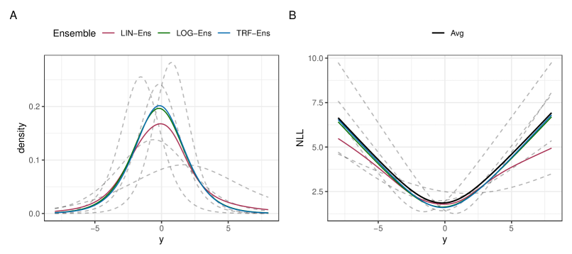
Figure 3: Illustration of linear (LIN-Ens), log-linear (LOG-Ens), and transformation (TRF-Ens) ensemble densities (A) and negative log-densities (B). Five logistic densities (dashed lines) are aggregated into an ensemble using the approaches outlined above.

An important question is whether increasing flexibility of the model class in classical ensembling is necessary for the commonly observed benefits in prediction performance. If the increased model complexity was necessary, transformation ensembles would not be able to compete with the classical ensembles, because they remain in the same model class as their members. In Section 5 we present empirical evidence that the increased complexity is not necessary. All types of ensembles show considerable improvement over the average performance of their members, but all types of ensemble perform roughly on par.

Even when using classical ensembles with transformation models as members, we can use the transformation ensemble approach to judge whether the ensemble deviates from the structural assumptions of its members. To do so, we transform the $M$ predicted CDFs to the scale of the empirical transformation function, $\{h_{m}(y_{i}\,|\,\text{\boldmath$x$}_{i})=F_{Z}^{-1}\circ F_{m}(y_{i}\,|\,\text{\boldmath$x$}_{i})\}_{i=1}^{n}$, and plot those against the likewise transformed ensemble predictions $\{F_{Z}^{-1}\circ\bar{F}_{M}(y_{i}\,|\,\text{\boldmath$x$}_{i})\}_{i=1}^{n}$, where $\bar{F}_{M}(y_{i}\,|\,\text{\boldmath$x$}_{i})$ is for example the classical linear ensemble (see Fig. 4 A). Observations close to the diagonal indicate that the ensemble does not deviate far from the model class of its members. In this example, notable deviations from the diagonal can be observed for smaller values of $y$, indicating the classical ensemble deviates from the model class of the members, which assumes additivity on the probit scale.

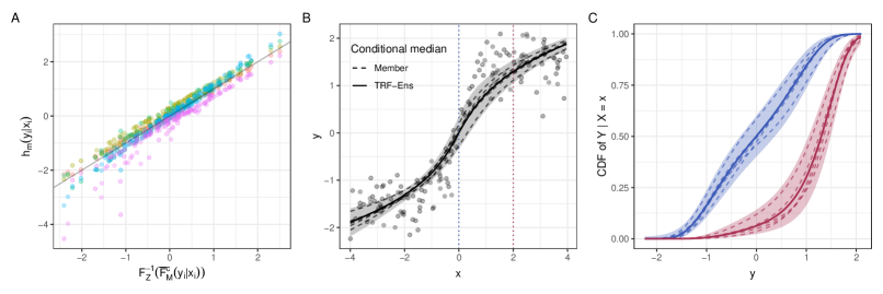
Figure 4: Transformation ensemble approach for checking model structure and quantifying uncertainty. A: Visual comparison of how far an ensemble deviates from the model class of its members on the scale of $F_{Z}^{-1}$, in this case the probit scale. B: Epistemic uncertainty of the transformation ensemble (TRF-Ens) in predicting the conditional median of $Y\,|\,x$. C: Epistemic uncertainty in the conditional distribution of $Y\,|\,X$ is displayed for $X=0$ (blue) and $X=2$ (red). Individual members are shown as gray dashed lines, and the transformation ensemble CDF with point-wise epistemic uncertainty as solid black lines. The data to produce this figure were simulated from the model $Y=3\operatorname{expit}(3x)+\epsilon$, where $\epsilon\sim\operatorname{N}(0,0.6^{2})$.

Uncertainty quantification

We now pose the related question of whether increasing model complexity via classical ensembling is necessary for the frequently noted improvement in epistemic uncertainty quantification in the classical ensemble. Transformation ensembles yield epistemic uncertainty estimates on the scale of the transformation function. Epistemic uncertainty can be displayed, for instance, when predicting the conditional $\alpha$-quantile, $\bar{q}_{M}(\text{\boldmath$x$};\alpha):=\bar{h}_{M}^{-1}(F_{Z}^{-1}(\alpha)\,|\,\text{\boldmath$x$})$. In Fig. 4 B, we show the conditional median, i.e., $\alpha=0.5$, as a point estimate along with the point-wise standard deviation $\bar{q}_{M}(\text{\boldmath$x$};0.5)\pm 2\operatorname{sd}(q_{m}(\text{\boldmath$x$};0.5))$ as a shaded area in the scatter plot of $y$ versus $x$. For the prediction at a single $x$, the epistemic uncertainty can also be transformed back to the CDF scale (Fig. 4 C). Here, the epistemic uncertainty is depicted as $F_{Z}(\bar{h}_{M}\pm 2\operatorname{sd}(h_{m}))$, where $\operatorname{sd}(h_{m})$ denotes the point-wise standard deviation of the predicted transformation functions $h_{m}$. Besides uncertainty in function space (transformation function, CDF, conditional median), transformation ensembles also yield epistemic uncertainty for the parameter space of additive linear predictors. For instance, if the model includes $\text{\boldmath$x$}^{\top}\text{\boldmath$\beta$}$, one can compute the epistemic uncertainty for each $\beta_{p}$, $p=1,\dots,P$ using asymptotic or bootstrap confidence intervals.

A major advantage of ensembling distributional regression models which are fitted using a loss derived from a proper score is that the members already quantify aleatoric uncertainty. Calibration of single models assesses how well the model quantifies aleatoric uncertainty. A model is (strongly) calibrated if its predictions match the population frequency of events, i.e., if $\mathbb{P}(Y\leq y\,|\,\hat{F})=\hat{F}(y)$. Calibration of ensembles assess overall uncertainty, i.e., both types of uncertainty, aleatoric and epistemic, simultaneously.

Minimax optimality

Commonly practitioners aim for the best performing model. However, in many applications optimal worst-case prediction errors are sought (e.g., in robust statistics, Huber, 2004). For instance, in forecasting extreme weather events practitioners may be willing to sacrifice average prediction performance to mitigate worst-case prediction errors (Gumbel, 1958). There is a strong similarity between transformation ensembles in eq. (5) and quasi-arithmetic pooling in eq. (1), for which minimax properties were shown for nominal outcomes (Neyman and Roughgarden, 2021). While quasi-arithmetic pooling is defined for densities of nominal outcomes, transformation ensembles act on the CDF of outcomes with an ordered sample space. However, for the special case of binary outcomes both aggregation methods coincide. Hence, for binary outcomes transformation ensembles are guaranteed to minimize worst-case prediction error in terms of NLL. The result follows from Theorem 4.1 in Neyman and Roughgarden (2021).

Corollary 1 (Minimax optimality of transformation ensembles).

Let $p_{1},\dots,p_{M}$ be predicted probabilities for success in a binary outcome, i.e., $p_{m}=\mathbb{P}_{m}(Y=1\,|\,\mathcal{D})$ and $w_{1},\dots,w_{M}$ be non-negative weights summing to one. Then $\bar{p}_{M}^{t}=\operatorname{expit}(\sum_{m}w_{m}\operatorname{logit}(p_{m}))$ minimizes

$$\max_{y}\operatorname{NLL}(p,y)-\sum_{m=1}^{M}w_{m}\operatorname{NLL}(p_{m},y).$$

In words, transformation ensembles for binary outcomes with $F_{Z}=\operatorname{expit}$ (standard logistic) are minimax optimal w.r.t. the NLL. Note that the result is independent of the type of ensemble members, i.e., for minimax optimality to hold, the members do not need to be transformation models. The proof of Corollary 1 is given in Appendix C. There, we also prove minimax optimality of linear pooling in terms of RPS and Brier score.

4 Experimental setup

We evaluate transformation ensembles in terms of prediction performance and calibration on several publicly available, semi-structured data sets with nominal, binary, and ordinal outcomes. We compare transformation ensembles, that preserve structure and interpretability of its members, to state-of-the-art ensembling methods (linear, log-linear ensembles, see Section 2.1) where the structure of the members is not preserved. In the following, we describe the different data sets and models used in our experiments.

4.1 Data sets

Melanoma

The publicly available melanoma data set (International Skin Imaging Collaboration, 2020) contains skin lesion color images of dimension $128\times 128\times 3$ along with age information of 33’058 patients. The response is binary and highly imbalanced (98.23% of all skin lesions are benign and 1.77% malignant).

UTKFace

The publicly available UTKFace data set contains facial images from people of various age groups. Here, age is treated as an ordinal outcome using seven categories, 0–3 ($n=1^{\prime}894$), 4–12 ($n=1^{\prime}519$), 13–19 ($n=1^{\prime}180$), 20–30 ($n=8^{\prime}068$), 31–45 ($n=5^{\prime}433$), 46–61 ($n=3^{\prime}216$) and $>61$ ($n=2^{\prime}395$) (Das et al., 2018). In addition, the data set contains sex (female, male) as a feature. To compare against the results reported in Kook et al. (2022), we use the same cropped version of the images reported therein. We simulate 10 additional covariates using the same simulation scheme as in Kook et al. (2022) with effect sizes $\pm\log 1.2$ for $X_{\{2,3\}}$, $\pm\log 1.5$ for $X_{\{5,6\}}$, and $0$ for the remaining covariates.

MNIST

The MNIST data set is a publicly available data set (LeCun et al., 2010) containing 60’000 gray-scaled training images of handwritten digits ranging from 0 to 9 with dimension $28\times 28$. In order to be able to define a CDF for the outcome, we arbitrarily fix the order to $0,1,\dots,9$. We choose to present results for the MNIST data set, to illustrate that the transformation ensemble approach is applicable to unordered outcomes too. All results for the MNIST data set are presented in Appendix E.

4.2 Models

For all data sets, we train several (ordinal) neural network transformation models (see Section 2.3) of varying intrinsic interpretability and flexibility. The data sets feature nominal, binary, and ordinal outcomes, all of which can be handled by ontrams.

Table 1: Overview of data sets, outcomes, and models fitted thereon. MNIST features a nominal outcome, for which we fit the most flexible CI_B model. The melanoma data set comes with a binary outcome for which we can fit a semi-structured model (CI_B-LS${}_{\text{\boldmath$x$}}$), two models using only one of the two modalities, and the unconditional model (SI). For UTKFace, age is split into ordered categories and several models of varying complexity are fitted. All models use $F_{Z}=\operatorname{expit}$ as the target distribution and hence all components of the transformation function are interpretable on the log-odds scale. CI: Complex intercept. CS: Complex shift. SI: Simple intercept. LS: Linear shift. A subscript indicates the input data for a model term, e.g., CS_B is a neural network with image input modelling a complex shift effect.

Data set	Outcome	Type	Model name	Transformation function
Melanoma	benign/malign	Binary	CIB-LS${}_{\text{\boldmath$x$}}$	$\vartheta(\mathsf{B})-\text{\boldmath$x$}^{\top}\text{\boldmath$\beta$}$
			CIB	$\vartheta(\mathsf{B})$
			SI-LS${}_{\text{\boldmath$x$}}$	$\vartheta-\text{\boldmath$x$}^{\top}\text{\boldmath$\beta$}$
			SI	$\vartheta$
UTKFace	age groups	Ordinal	CIB-LS${}_{\text{\boldmath$x$}}$	$\vartheta_{k}(\mathsf{B})-\text{\boldmath$x$}^{\top}\text{\boldmath$\beta$}$
			SI-CSB-LS${}_{\text{\boldmath$x$}}$	$\vartheta_{k}-\eta(\mathsf{B})-\text{\boldmath$x$}^{\top}\text{\boldmath$\beta$}$
			CIB	$\vartheta_{k}(\mathsf{B})$
			SI-CSB	$\vartheta_{k}-\eta(\mathsf{B})$
			SI-LS${}_{\text{\boldmath$x$}}$	$\vartheta_{k}-\text{\boldmath$x$}^{\top}\text{\boldmath$\beta$}$
			SI	$\vartheta_{k}$
MNIST	Digits 0–9	Nominal	CIB	$\vartheta_{k}(\mathsf{B})$

The degree of intrinsic interpretability can be controlled by parametrizing the transformation function in different ways (see Table 1). We follow the model nomenclature in Kook et al. (2022), where transformation functions consist of an intercept (SI: simple intercept, i.e., intercepts do not depend on input data, CI: complex intercept, intercepts depend on input data) and potentially shift terms (LS: linear shift, additive linear predictor of tabular features, CS: complex shift, additive but flexible predictor depending on either tabular or image data). A subscript indicates which part of the model depends on which input modality. Note that for models with binary outcomes, the CI_B and SI-CS_B are equivalent, unless the complex shift term is restricted to have mean zero. Therefore, we only fit the CI_B version of these models which are reparametrizations of classical image convolutional networks with softmax last-layer activation.

Training

All models were fitted by minimizing NLL or RPS, both of which are proper scores (Section 2.2). In contrast to NLL, RPS is a global score which is bounded and explicitly takes the natural order of the outcome into account. For binary responses, RPS reduces to the Brier score. We apply all ensemble methods to five instances of the same model for six random splits of each data set. Training procedures and model architectures are described in Appendix B in more detail.

Tuning ensemble weights

Instead of equal weighting or top-$K$ ensembling, one can tune the ensemble weights such that the prediction performance w.r.t. a proper score is optimized on a hold-out data set. Tuning the composition of an ensemble in such a way is related to stacking (Wolpert, 1992; Breiman, 1996b). The hold-out set could be the validation set when splitting the data randomly or the validation fold during a $k$-fold cross-validation. Concretely, we choose the weights by solving

$$\begin{split}\min_{w\geq 0}&\sum_{i=1}^{n}s(\bar{F}_{M,i}^{w},y_{i}),\\ \mbox{s.t. }&\sum_{m}w_{m}=1,\end{split}$$ (6)

for some proper score $s$ and predictions from the weighted ensemble $\bar{F}_{M,i}^{w}$.

Evaluation

For all data sets, we evaluate the prediction performance via proper scores (NLL, RPS or BS, Section 2) and discriminatory performance (accuracy, AUC and Cohen’s quadratic weighted kappa). We investigate uncertainty quantification of individual models and ensembles using calibration plots. In addition, we report calibration in the large and calibration slope in Appendix E. For nominal and ordinal outcomes, these calibration metrics are computed per class. See Appendix B for the exact definitions of the above metrics.

5 Results and discussion

We apply linear, log-linear, and transformation ensembling to three data sets with a nominal, binary, and ordered outcome, respectively (see Section 4.1). We refer to the three ensemble types as LIN-Ens, LOG-Ens, and TRF-Ens in all figures, respectively. The focus of the comparison is on the performance difference between ensemble types, but also between the different models, which vary in their degree of flexibility and interpretability (see Tab. 1). Average ensemble test performance and bootstrap confidence intervals based on six random splits of the data are shown for all models. Beside prediction performance, we discuss interpretability and calibration of the different models and ensembles.

Melanoma

Four models of different flexibility and interpretability are fitted (see Table 1) with the melanoma data in order to predict the conditional probabilities of the unbalanced binary outcome benign or malignant lesion given a person’s age and an image of the skin lesion.

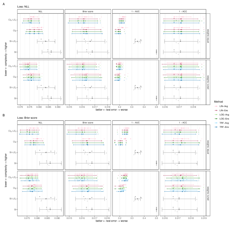
Figure 5: Performance estimates on the melanoma data set. The classical linear (LIN-Ens), classical log-linear (LOG-Ens), and transformation (TRF-Ens) ensemble test error is shown for negative log-likelihood (NLL), Brier score, discrimination error ($1-\operatorname{AUC}$) and classification error ($1-\operatorname{ACC}$). The average ensemble test error and 95% bootstrap confidence intervals are depicted for six random splits (indicated by different symbols) of the data. In the upper panels ensemble members are weighted equally and in the lower panels weights are tuned to minimize validation loss. In case of equal weights, the average coincides for all ensemble types (LIN-Avg). Models are fitted by minimizing NLL (A) or Brier score (B). Note the different scales for A and B.

We now see empirically that all ensemble methods (LIN-Ens, LOG-Ens, TRF-Ens) result in a higher test performance w.r.t. the two proper scores NLL (as shown in Prop. 3) and RPS compared to their members’ average (Avg, see Fig. E1). When additionally tuning the ensemble weights on the validation set, test prediction and discrimination performance improve further. Test performance indicates for all ensemble methods that both input modalities, a person’s age and appearance of the lesion, aid in predicting the risk of a malignant vs. a benign skin lesion (see Fig. 5). While the image data (CI_B) seems to be most important for prediction, including age (CI_B-LS${}_{\text{\boldmath$x$}}$) further improves prediction performance (NLL, Brier score). The unconditional model (SI) achieves a NLL and Brier score close to that of the model (SI-LS${}_{\text{\boldmath$x$}}$) based on age alone. However, SI-LS${}_{\text{\boldmath$x$}}$ lacks in discriminatory ability (AUC), which suggests that the seemingly high performance of the unconditional model is due to the highly imbalanced outcome. Performance of the individual ensemble members and performance relative to the SI-LS${}_{\text{\boldmath$x$}}$ model are shown in Appendix E.

For the best performing CI_B-LS${}_{\text{\boldmath$x$}}$ model all three ensemble methods improve compared to the average performance of the individual models and result in similarly low test error (NLL, Brier score). The positive effect of optimizing the ensemble weights seems to be more pronounced when there is more variation in the individual members’ performance (note the larger benefit for the CI_B model than for the CI_B-LS${}_{\text{\boldmath$x$}}$ model in Fig. E4). A reduction in between-split variation is observed, when tuning the ensemble weights. Whether NLL or Brier score is optimized during training influences test performance only slightly for this data set. Especially for AUC, optimizing NLL instead of Brier score yields slightly better results (compare Fig. 5 A and B).

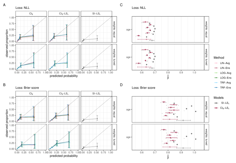
Figure 6: Calibration plots (A and B) and coefficient estimates (C and D) for different models fitted on the melanoma data set. Calibration with 95% confidence intervals averaged across splits are depicted for the classical linear (LIN-Ens), classical log-linear (LOG-Ens), and transformation (TRF-Ens) ensemble in A and B. The predicted probabilities for a malign lesion are split at four empirical quantiles (0.5, 0.9, 0.99, 0.999) to compute the proportion of a malign lesion in the five resulting bins. For the SI-LS${}_{\text{\boldmath$x$}}$, the last two bins are merged. Panels C and D show log odds-ratios ($\hat{\beta}$) and 95% bootstrap confidence intervals for the standardized age predictor in the models SI-LS${}_{\text{\boldmath$x$}}$ and CI_B-LS${}_{\text{\boldmath$x$}}$ for each of the six random split. The average log odds-ratio across splits is shown as transparent diamond along with a 95% confidence interval. Individual log odds-ratios of the five ensemble members in each split are shown as transparent dots for the model CI_B-LS${}_{\text{\boldmath$x$}}$. In the upper panels ensemble members are weighted equally and in the lower panels weights are tuned to minimize validation loss.

Calibrated predictions are hard to achieve when the outcome is highly imbalanced. For predicted probabilities below $0.2$, all models seem to be well calibrated (Fig. 6 A and B). However, the SI-LS${}_{\text{\boldmath$x$}}$ model over-predicts the probability for the rare outcome (malign lesion). Note that the last bin includes only 0.1% of observations and the model never predicts probabilities of a malign lesion larger than 0.13. When including the image data, calibration improves somewhat and uncertainty increases. Again, there is no pronounced difference between equal and tuned weights, ensemble types, and ensembles and individual members, or NLL and Brier score loss. Calibration-in-the-large and calibration slope estimates are shown in Appendix E.

Lastly, since age is included as a tabular predictor, individual models and transformation ensembles thereof produce directly interpretable estimates for the log odds of a malign vs. a benign lesion upon increasing age by by one standard deviation (Fig. 6 C and D). In all models, increasing age is associated with a higher risk of the lesion being malign. In transformation ensembles, the pooled estimate is simply the (weighted) average of the members’ estimates. Note that the log odds-ratios obtained by minimizing NLL and RPS agree in direction, but differ slightly in magnitude. In particular, the maximum RPS solution in SI-LS${}_{\text{\boldmath$x$}}$ is more uncertain than the maximum likelihood solution (grey dots in Fig. 6 C vs. D).

UTKFace

We fit six models of different flexibility and interpretability (see Table 1) to the UTKFace data in order to predict the conditional distribution of age categories given a person’s face and/or sex and simulated tabular data. Fig. 7 shows the average ensemble test error with bootstrap confidence intervals for four more complex models (CI_B-LS${}_{\text{\boldmath$x$}}$, CI_B, SI-CS_B-LS${}_{\text{\boldmath$x$}}$, SI-CS_B) and each ensembling method.

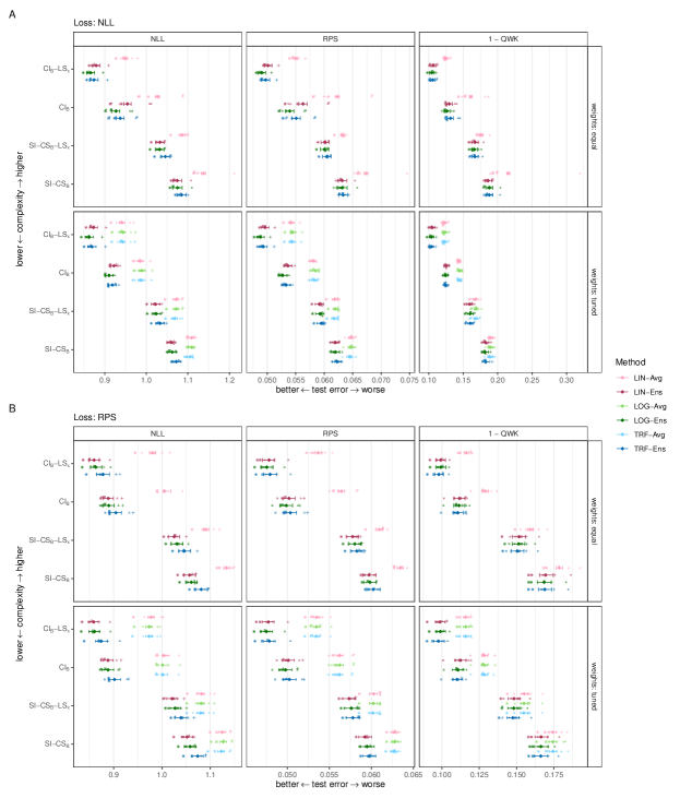
Figure 7: Performance estimates on the UTKFace data set. The classical linear (LIN-Ens), classical log-linear (LOG-Ens), and transformation (TRF-Ens) ensemble test error is shown for negative log-likelihood (NLL), ranked probability score (RPS) and discrimination error measured by Cohen’s quadratic weighted kappa ($1-\operatorname{QWK}$). The average ensemble test error and 95% bootstrap confidence intervals are depicted for six random splits (indicated by different symbols) of the data. In the upper panels ensemble members are equally weighted for constructing the ensemble and in the lower panels weights are tuned to minimize validation loss. In case of equal weights, the average coincides for all ensemble types (LIN-Avg). Models are fitted by minimizing NLL (A) or RPS (B). Note the different scales for A and B. The results for the SI and SI-LS${}_{\text{\boldmath$x$}}$ models are shown in Appendix E.

Test performance of the two simplest models (SI, SI-LS${}_{\text{\boldmath$x$}}$) can be found in the Appendix E along with the estimated coefficients for age and the ten simulated tabular predictors. Performance of the individual ensemble members and performance relative to the SI-LS${}_{\text{\boldmath$x$}}$ model are shown in Appendix E.

Similar to the results found in Kook et al. (2022) the most flexible model including both image and tabular data (CI_B-LS${}_{\text{\boldmath$x$}}$) performs best across both proper scores and discrimination metrics. Assuming proportional odds for the image term does not seem to be appropriate, given the improved prediction performance when loosening this assumption (CI_B-LS${}_{\text{\boldmath$x$}}$ vs. SI-CS_B-LS${}_{\text{\boldmath$x$}}$ and CI_B vs. SI-CS_B). All models including the image data perform considerably better than the benchmark model including only tabular data (SI-LS${}_{\text{\boldmath$x$}}$, see Fig. E7).

When comparing the different ensembling methods we again observe comparable performance of the transformation ensemble to that of the classical ensembles for all test metrics. This difference is even more pronounced when ensemble weights are tuned to minimize validation loss (lower panels of Fig. 7). As observed in the other data sets, tuning the ensemble weights reduces the variability in performance. As expected, models fitted by minimizing the RPS result in a lower test RPS. However, the NLL of these models is also on par with or even better than when optimizing the NLL. This provides some empirical evidence that optimizing the RPS may lead to more stable training for ordered outcomes, because it is bounded and global (Gneiting et al., 2005).

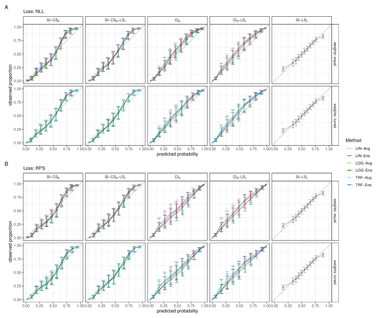
Figure 8: Calibration plots for different models fitted on the UTKFace data set. The average calibration across 6 random splits and 95% confidence intervals are depicted of the classical linear (LIN), classical log-linear (LOG), and transformation (TRF) ensemble. The predicted probabilities are split at the 0.5, 0.95 quantiles and nine equidistant cut points in-between to calculate the observed event rate in each bin. In the upper panels ensemble members are equally weighted for constructing the ensemble and in the lower panels weights are tuned to minimize validation loss. Models are fitted by minimizing NLL (A) or RPS (B).

On the UTKFace data, models are fairly calibrated after training. The SI-LS${}_{\text{\boldmath$x$}}$ model, including only tabular data, over-predicts large probabilities. Upon including image data as complex intercepts, calibration again improves notably (CI_B, CI_B-LS${}_{\text{\boldmath$x$}}$), whereas under-prediction can be observed when modelling image contributions as complex shifts (SI-CS_B, SI-CS_B-LS${}_{\text{\boldmath$x$}}$). This can again be interpreted as evidence that assuming proportional odds is unreasonable for this data set. CI_B and CI_B-LS${}_{\text{\boldmath$x$}}$ models are better calibrated when fitted with the RPS loss. Again, no pronounced difference could be observed between the the two weighting schemes, or between ensembles and individual models. However, the log-linear ensemble produces the best-calibrated predictions in the CI_B and CI_B-LS${}_{\text{\boldmath$x$}}$ models. Calibration-in-the-large and calibration slope estimates are shown in Appendix E.

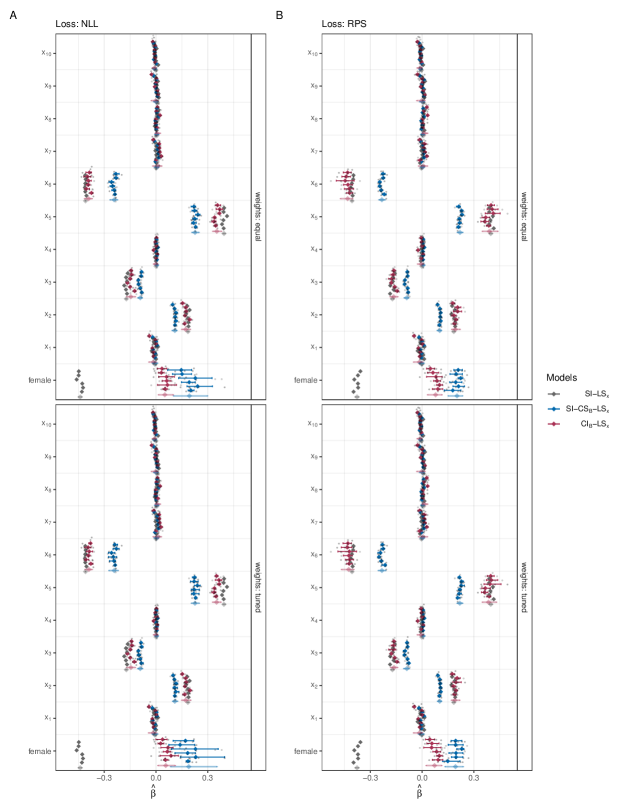
Figure E10: Coefficient estimates on the UTKFace data set. Average log odds-ratios ($\hat{\text{\boldmath$\beta$}}$) and 95% bootstrap confidence intervals of belonging to a higher age class when increasing one of the 10 simulated predictors by one unit or switching from male to female for each random split. The average log odds-ratio across splits is shown as transparent dot for each model. Individual odds ratios of all $5\times 6$ ensemble members or six splits for the SI-LS${}_{\text{\boldmath$x$}}$ model, respectively, are shown as gray dots. In the upper panels ensemble members were equally weighted for constructing the ensemble and in the lower panels weights were tuned to minimize validation loss. Models were trained by minimizing NLL (A) or RPS (B).

For the ten simulated tabular predictors and sex the individual models with linear shift terms and the corresponding transformation ensemble yield directly interpretable log odds-ratios. In Figure E10, estimated log odds-ratios are depicted together with bootstrap confidence intervals. The CI_B-LS${}_{\text{\boldmath$x$}}$ models’ estimates are close to the estimates of the SI-LS${}_{\text{\boldmath$x$}}$ models, whereas the estimates of the SI-CS_B-LS${}_{\text{\boldmath$x$}}$ model experience some shrinkage. The estimate for sex (female) changes sign upon inclusion of the image data, potentially due to collinearity between learned image features and the tabular indicator variable. Again, the weighted average of the ensemble members’ estimated coefficients is in fact the estimate in the transformation ensemble, which is not the case for any other type of ensemble discussed in this paper.

MNIST

Results for the MNIST data set can be found in Appendix E.

6 Summary and outlook

Transformation ensembles bridge the gap between two common goals, prediction performance and interpretability. Not only are they guaranteed to score better than their ensemble members do on average, but in addition they preserve model structure and thus possess the same intrinsic interpretability as their members. As a consequence, transformation ensembles allow to directly assess epistemic uncertainty in the intrinsically interpretable model parameters. On multiple data sets we demonstrate that transformation ensembles improve both probabilistic and discriminatory performance measures. Transformation ensembles perform on par with classical ensembling approaches on all three datasets. Thus transformation ensembles present a viable alternative to classical ensembling in terms of prediction and discrimination.

Preserving the intrinsic interpretability of its members is the most crucial benefit of transformation ensembles. Practitioners in fields where decisions are commonly based on multimodal and semi-structured data, such as medicine, require transparent, well-performing and intrinsically interpretable models (Rudin, 2019). As our results suggest, the increased flexibility of the model class when using classical ensemble techniques may often not be necessary. Instead, the more interpretable transformation ensemble performs at least on par. In addition, transformation ensembles simply pool interpretable model parameters in additive linear predictors using a (weighted) average. This does not only yield transformation ensembles with the same model structure and interpretability, but also allows to assess the epistemic uncertainty in linear shift terms. This is in line with intuition but without theoretical justification when using any other type of ensemble. For complex shift and complex intercept terms which are not intrinsically interpretable, data analysts may still use transformation ensembles and apply post hoc explainability methods to those model components (Molnar, 2020, Ch. 6).

Transparency requires clear communication of data and model uncertainty. Transformation ensembles provide epistemic uncertainty estimates both in function space (transformation function, CDF, or conditional quantiles) and parameter space (parameters of additive linear predictors). We use ensemble calibration to judge the quality of both aleatoric and epistemic uncertainty simultaneously. In terms of calibration, no ensemble type led to a pronounced improvement over individual models’ average. For both data sets including tabular data (melanoma, UTKFace), including the images alongside tabular data improved calibration. In clinical prediction modelling, where calibrated predictions are of high importance, it may thus be advantageous to model image contributions or to aggregate re-calibrated (Steyerberg, 2019, Ch. 15.3.5) versions of the models.

Optimizing the ensemble weights on a hold out set, is a simple way to reduce variability between random splits of the data. If only little data is available for training, a cross validation scheme may yield similar benefits when averaging the weights over the cross validation folds.

In this article, we mainly focused on interpretability, prediction and calibration. Apart from benefits in prediction performance and uncertainty quantification, deep ensembles have found to be robust when evaluated out of distribution, e.g., under distributional shifts (for a discussion, see Abe et al., 2022). We leave for future research how transformation ensembles compare to classical linear ensembling in terms of robustness towards distributional shifts and related issues in epistemic uncertainty estimation. Further theoretical directions include whether minimax optimality of transformation ensembles for binary outcomes extends to ordered and continuous outcomes.

Acknowledgements

We thank Jeffrey Adams, Oliver Dürr, Lisa Herzog, David Rügamer and Kelly Reeve for their valuable comments on the manuscript. The research of LK and BS was supported by Novartis Research Foundation (FreeNovation 2019) and by the Swiss National Science Foundation (grant no. S-86013-01-01 and S-42344-04-01). TH was supported by the Swiss National Science Foundation (SNF) under the project “A Lego System for Transformation Inference” (grant no. 200021_184603).

Appendix A Notation

Random variables are written in uppercase italic, $Y$, and realizations thereof in lowercase, $y$. In case, the random variable is vector-valued, we write it and its realizations in bold, e.g., $X$, $x$. We denote probability measures by $P$, PDFs by $f$ and CDFs by $F$. Ensemble members are denoted by $F_{m}$, or $f_{m}$, $m=1,\dots,M$, when referring to the CDF or PDF, respectively. An ensemble is some average of these members and its CDF and PDF are denoted by $\bar{F}_{M}$, $\bar{f}_{M}$, respectively. A superscript then denotes the type of ensemble, e.g., $\bar{F}_{M}^{c}$ the classical linear ensemble. If, for two functions $f,g:A\to B$, $f(a)\leq g(a)$ for all $a\in A$, we omit the argument and write $f<g$.

Appendix B Computational details

The code for reproducing all experiments can be found on GitHub https://github.com/LucasKook/interpretable-deep-ensembels. All components of the models used in this work (see Table 1 for an overview) were controlled by neural networks and fitted jointly by minimizing the negative log-likelihood or ranked probability score via stochastic gradient descent using the Adam optimizer [Kingma and Ba, 2015]. The unconditional model (SI) and the model containing tabular predictors only (SI-LS${}_{\text{\boldmath$x$}}$) were fitted using the function tram::Polr [Hothorn, 2020] in case of ordinal responses and stats::glm in case of binary responses. Both models were also implemented as ontrams to minimize the RPS. Factor variables were dummy encoded and continuous predictors were standardized to zero mean and unit variance. All models were implemented in R [R Core Team, 2021, version 4.1.1]. Semi-structured data was modeled using Keras [Allaire and Chollet, 2021, version 2.7.0] based on the TensorFlow backend [Allaire and Tang, 2021, version 2.7.0] and trained on a GPU.

Simple intercept terms (and the SI model) were estimated using a fully-connected single-layer neural network with linear activation function, no bias term, and $K-1$ output nodes. Linear shift terms (LS${}_{\text{\boldmath$x$}}$) were estimated similarly but with a single output node. Both, simple intercept and linear shift terms were initialized using the parameters estimated by either a proportional odds logistic regression model (POLR) or a generalized linear model (GLM).

Terms depending on the image modality (CI_B, CS_B) were modeled using a 2D convolutional neural network (CNN) for all data sets. The last layer was common to all CNNs and consisted of either $K-1$ output nodes for complex intercept terms or a single output node for complex shift terms. The identity was used as activation (ReLU non-linearity was used in all other layers) and no bias term was included. In case of intercept terms, the raw intercepts $\gamma\in\mathbb{R}^{K-1}$ were further transformed to the intercepts $\vartheta$ via a cumulative softplus transformation

$$\text{\boldmath$\vartheta$}=\left(\gamma_{1},\gamma_{1}+\log(1+\exp(\gamma_{2})),\dots,\gamma_{1}+\sum_{k=2}^{K-1}\log(1+\exp(\gamma_{k}))\right),$$

to ensure monotonicity. The CNNs used to control complex model terms (CI_B, CS_B) were initialized as Glorot uniform, and zero bias. To prevent the models from overfitting, weights from the epoch with the smallest validation loss were used as the final model. For all data sets, images were normalized to the unit interval via $(y-\min(y))/(\max(y)-\min(y))$. No further pre-processing steps were undertaken.

For all data sets, the data was randomly split six times into a training, validation and a test set. Five models trained and evaluated on the same split built an ensemble. Hyperparameters, such as the number of training epochs or the weights for constructing the weighted ensemble, were tuned on the validation set. In applications it may be advised to use a nested cross-validation scheme instead of tuning on a single validation set. Model architectures and hyperparameters varied across data sets and will be described for each data set in the following.

MNIST

To predict the nominal outcome a CNN with three convolutional stacks consisting of a convolutional layer and a max-pooling layer (window size $2\times 2$ pixels, stride width $2$) was used. The number of filters used in each stack were $32$, $64$, $64$. Filter size was set to $3\times 3$ pixels. The fully-connected part comprised a layer with $100$ units followed by the output layer (see Fig. B1).

All 30 models (six ensembles consisting of five members each) were trained on 80% and validated on 10% of the data. Ensembles were validated on 10% of the data. A learning rate of $10^{-5}$ and a batch size of $512$ were used for model training.

Figure B1: CNN architecture used for the MNIST, melanoma, and UTKFace data.

Melanoma

CI_B and CS_B terms were modeled using a CNN with two convolutional stacks with $16$ filters ($3\times 3$ pixels) and two convolution stacks with $32$ filters ($3\times 3$ pixels). Each convolutional layer was followed by a dropout layer (rate $0.3$) and a max-pooling layer (window size $2\times 2$ pixels, stride width $2$). For the subsequent fully-connected part, two dense layers with $256$ and $64$ units and two dropout layers (rate $0.3$) were used (see Fig. B1).

Models were trained on 60%, validated on 20% and evaluated on 20% of the data. CNNs were trained using a learning rate of $10^{-4}$ and a batch size of 64.

UTKFace

A similar CNN architecture as in Kook et al. [2022] was used to incorporate the image modality (Fig. B1). The architecture was originally inspired by Simonyan and Zisserman [2014]. The model is given by three convolutional stacks of which each consists of two convolutional layers, two dropout layers (rate $0.3$) and a max-pooling layer (window size $2\times 2$ pixels, stride width $2$). In the first two convolutional stacks $32$ filters were used followed by two stacks using $64$ filters ($3\times 3$ pixels). After flatting, the output entered the fully connected part comprised of two dense layers separated by a dropout layer (rate $0.3$).

All models were trained on 60%, validated on 20% and evaluated on 20% of the data. CNNs were trained using a learning rate of $10^{-3}$ and a batch size of 32.

Evaluation metrics

Classification metrics depend on the (top-label) classification, which we define as the mode of the predicted conditional density, i.e.,

$$c=\operatorname*{{arg\,max}}_{k}f(y_{k}\,|\,\mathcal{D}),$$

from which we then compute the accuracy

$$\operatorname{ACC}=\frac{1}{n}\sum_{i=1}^{n}\delta_{y_{i}}^{c_{i}},\mbox{ where }\delta_{a}^{b}=\begin{cases}1&\mbox{if }a=b\\ 0&\mbox{otherwise},\end{cases}$$

and Cohen’s quadratic weighted $\kappa$,

$$\kappa_{w}=\frac{\sum_{i,j}w_{ij}o_{ij}-\sum_{i,j}w_{ij}e_{ij}}{1-\sum_{i,j}w_{ij}e_{ij}}.$$

Here, $e$ and $o$ denote the expected and observed number of agreements in row $i$ and column $j$ of a confusion matrix, respectively. In addition, the weights $w_{ij}=\frac{\lvert i-j\rvert^{q}}{(K-1)^{p}}$ control the penalization for predictions farther away from the observed class via $q$.

The AUC is a discrimination metric, defined as

$$\operatorname{AUC} =\max\{\operatorname{PI},1-\operatorname{PI}\},\mbox{ where }$$

$$\operatorname{PI} =\mathbb{P}(Y_{1}<Y_{2}\,|\,\mathcal{D}_{1},\mathcal{D}_{2})+\frac{1}{2}\mathbb{P}(Y_{1}=Y_{2}\,|\,\mathcal{D}_{1},\mathcal{D}_{2}).$$

Here, PI denotes the probabilistic index and $Y_{1}\,|\,\mathcal{D}_{1}$ and $Y_{2}\,|\,\mathcal{D}_{2}$ are independent and distributed according to $F_{Y\,|\,\mathcal{D}}$ [Thas et al., 2012].

Lastly, we use calibration plots and compute two calibration metrics, calibration in the large and calibration slope [Steyerberg, 2019]. Calibration plots are produced using the caret add-on package for R [Kuhn, 2022]. Confidence intervals are obtained via standard binomial tests and averaged over splits. The calibration slope $b_{1}$ is obtained by regressing the indicator for a class on the predicted log odds for that class,

$$\operatorname{logit}(\mathbb{E}[\mathds{1}(Y>y_{k})\,|\,\hat{r}_{k}])=b_{0}+b_{1}\hat{r}_{k},$$

where $\hat{r}_{k}=\operatorname{logit}(\hat{\mathbb{P}}(Y>y_{k}\,|\,\mathcal{D}))$. Similarly, calibration in the large $a$, is the intercept in the model offsetting the predicted log odds $\hat{r}_{k}$,

$$\operatorname{logit}(\mathbb{E}[\mathds{1}(Y>y_{k})\,|\,\hat{r}_{k}])=a+1\hat{r}_{k}.$$

Bootstrap confidence intervals

For each metric, we report bootstrap confidence intervals over $b=1,\dots,B=1^{\prime}000$ bootstrap samples of $i=1,\dots,n_{\rm test}$ test observations, for each of the $s=1,\dots,S=6$ splits and $m=1,\dots,M=5$ members, by taking the 2.5th and 97.5th empirical quantile of the bootstrap metric. For the three ensemble types, there is no step of averaging over the $M$ members. In case of relative performance, the fixed SI-LS${}_{\text{\boldmath$x$}}$ performance per split was subtracted instead of the bootstrap metric. To construct confidence intervals for the coefficient estimates, the $M$ member estimates were bootstrapped.

Appendix C Proofs and additional results

Proof of Proposition 3

We re-state Prop. 3. For the proof, we exploit the fact that in transformation models, $F_{Z}$ has a log-concave density.

Proposition.

Let $F_{Z}\circ h_{1},\dots,F_{Z}\circ h_{M}$ be transformation model CDFs with $w_{1},\dots,w_{M}$ non-negative weights summing to one. Let $\ell:\mathcal{P}\to\mathbb{R}$ denote the log-likelihood induced by the transformation model $F_{Z}\circ h$. Then, $-\ell\left(F_{Z}(\sum_{m}w_{m}h_{m})\right)\leq-\sum w_{m}\ell\left(F_{Z}\circ h_{m}\right)$.

Proof.

The log-density of the transformation ensemble is given by

$$\log\bar{f}_{M}^{t}(y)=\log\frac{\,\mathrm{d}}{\,\mathrm{d}y}F_{Z}\left(\sum_{m}w_{m}h_{m}(y)\right)=\log\left[f_{Z}\left(\sum_{m}w_{m}h_{m}(y)\right)\sum_{m}w_{m}h_{m}^{\prime}(y)\right].$$

Now, the result follows by applying Jensen’s inequality for both terms,

$$-\log f_{Z}\left(\sum_{m}w_{m}h_{m}\right)-\log\left(\sum_{m}w_{m}h_{m}^{\prime}\right)\leq-\sum_{m}w_{m}\log\left(f_{Z}\circ h_{m}\right)-\sum_{m}w_{m}\log h_{m}^{\prime},$$

once using log-concavity of $f_{Z}$ and once using concavity of the log.

In case of interval-censored responses (see Section 2), $y\in(\underaccent{\bar}{\ry},\bar{y}]$ the likelihood contribution,

$$-\log\left[F_{Z}\left(\sum_{m}w_{m}h_{m}(\bar{y})\right)-F_{Z}\left(\sum_{m}w_{m}h_{m}(\underaccent{\bar}{\ry})\right)\right],$$

is convex in $h_{m}$ because the transformation function is monotone non-decreasing and $\underaccent{\bar}{\ry}<\bar{y}$. The desired claim follows again via Jensen’s inequality. ∎

Similar results for the Brier score and RPS (a sum of Brier scores) do not hold for general $F_{Z}$, because log-concavity of $F_{Z}$ is not a strong enough condition to ensure convexity of $L\circ F_{Z}$.

Next, we briefly state and prove propositions for better-than-average prediction performance of the two variants of the log-linear ensemble (PDF and CDF pooling).

Proposition 4.

Let $f_{1},\dots,f_{M}$ be conditional densities with non-negative weights $w_{1},\dots,w_{M}$ summing to one. Let $\bar{f}_{M}=c\exp\left(\sum_{m}w_{m}f_{m}\right)$, where $c^{-1}:=\int_{-\infty}^{+\infty}\exp(\sum_{m}w_{m}\log f_{m})$. Then, $\operatorname{NLL}(\bar{f}_{M})\leq\sum_{m}w_{m}\operatorname{NLL}(f_{m})$.

Proof.

The ensemble NLL is given by $\operatorname{NLL}(\bar{f}_{M})=-\log c-\sum_{m}w_{m}\log f_{m}$, hence we need to show $c\geq 1$. Indeed, we have

$$c^{-1}=\int_{-\infty}^{+\infty}\exp\left(\sum_{m}w_{m}\log f_{m}\right)\leq\int_{-\infty}^{+\infty}\sum_{m}w_{m}f_{m}=1,$$

via Jensen’s inequality. ∎

Proposition 5.

Let $F_{1},\dots,F_{M}$ be conditional CDFs with non-negative weights $w_{1},\dots,w_{M}$ summing to one. Let $\bar{F}_{M}=\exp(\sum_{m}w_{m}F_{m})$. Then, $\operatorname{NLL}(\bar{f}_{M})\leq\sum w_{m}\operatorname{NLL}(f_{m})$, where $\bar{f}_{M}=\frac{\,\mathrm{d}}{\,\mathrm{d}y}\bar{F}_{M}=\exp(\sum_{m}\log F_{m})(\sum_{m}w_{m}f_{m}/F_{m})$.

Proof.

The ensemble NLL is given by

$$\operatorname{NLL}(\bar{f}_{M}) =-\sum_{m}w_{m}\log F_{m}-\log\left(\sum_{m}w_{m}f_{m}/F_{m}\right)$$

$$\leq-\sum_{m}w_{m}\log F_{m}-\sum_{m}w_{m}\log f_{m}+\sum_{m}w_{m}\log F_{m}$$

$$=-\sum_{m}w_{m}\log f_{m}=\sum_{m}w_{m}\operatorname{NLL}(f_{m}),$$

by Jensen’s inequality. ∎

Remark 1.

Propositions 4 and 5 illustrate that both log-linear ensembles of PDFs and CDFs produce better than average predictions. Normally densities are aggregated in log-linear ensembles. However, since we propose a CDF-based ensemble, the CDF version of the log-linear ensemble is a more direct comparator to transformation ensembles in our experiments.

Next, we present more results on minimax optimality of quasi-arithmetic pooling and transformation ensembles.

Proof of Corollary 1

First, we give some intuition. The approach by Neyman and Roughgarden [2021] can be inverted to find a (regular) proper scoring rule corresponding to a given pooling method. The transformation ensemble in general uses quasi-arithmetic pooling with $g=F_{Z}^{-1}$ on the CDF scale. Now, instead of finding the minimax optimal pooling for a score, we take the reverse route and construct

$$G(p)=\int_{0}^{p}F_{Z}^{-1}(u)\,\mathrm{d}u.$$ (7)

Eq. (7) is an integrated quantile function and has close connections to the expectation of $Z$ and trimmed expectations in general. This can be seen in $\mathbb{E}[Z]=\mathbb{E}[F_{Z}^{-1}(U)]=\int_{0}^{1}F_{Z}^{-1}(u)\,\mathrm{d}u$, where $U$ is standard uniform. Before we prove Corollary 1, we restate Theorem 4.1 from Neyman and Roughgarden [2021].

Theorem 1 (Minimax optimality, Theorem 4.1 in Neyman and Roughgarden [2021]).

Let $p_{1},\dots,p_{M}$ be probability densities for a nominal outcome, i.e., $p_{m}(y_{k})=\mathbb{P}_{m}(Y=y_{k})$, with non-negative weights $w_{1},\dots,w_{M}$ summing to one. Then

$$\max_{y}s(p,y)-\sum_{m=1}^{M}w_{m}s(p_{m},y)$$

is minimized by $p=g^{-1}(\sum_{m}w_{m}g(p_{m}))$, where $s$ is a proper score and $g$ is a subgradient of the expected score.

We now re-state and prove Corollary 1.

Corollary.

Let $p_{1},\dots,p_{M}$ be predicted probabilities for success in a binary outcome, i.e., $p_{m}=\mathbb{P}_{m}(Y=1\,|\,\mathcal{D})$ and $w_{1},\dots,w_{M}$ be non-negative weights summing to one. Then $\bar{p}_{M}^{t}=\operatorname{expit}(\sum_{m}w_{m}\operatorname{logit}(p_{m}))$ minimizes

$$\max_{y}\operatorname{NLL}(p,y)-\sum_{m=1}^{M}w_{m}\operatorname{NLL}(p_{m},y).$$

Proof.

For transformation ensembles with $F_{Z}=\operatorname{expit}$ and binary outcomes, we have for each member $p\in\{p_{1},\dots,p_{M}\}$,

$$G(p)=\int_{0}^{p}F_{Z}^{-1}(u)\,\mathrm{d}u=p\log p+(1-p)\log(1-p)+C=-\mathbb{E}[\operatorname{NLL}(p,Y)]+C.$$

The result then follows from Theorem 1. ∎

Thus we find that transformation ensembling with $F_{Z}=\operatorname{expit}$ is minimax optimal for binary outcomes in terms of NLL. Note that the restriction to binary outcomes is necessary, because Neyman and Roughgarden [2021] ensemble densities of nominal outcomes, for which the CDF is ill-defined. We aggregate predictions on the CDF scale, because this ensures interpretability of the transformation ensemble. In turn, the two approaches can only be equivalent for binary outcomes, for which the distribution is fully characterized by $\mathbb{P}(Y\leq y_{0})=\mathbb{P}(Y=y_{0})=p$ when defining the “order” of the binary outcome appropriately.

Minimax optimal pooling for the RPS

Neyman and Roughgarden [2021] present results solely for nominal outcomes, for which the CDF is not well-defined. However, we can still extend their results by considering linear pooling, for which the aggregation scale (CDF or PDF) does not matter. Then, we arrive at the following result.

Corollary 2 (Classical linear ensembling is minimax optimal i.t.o. RPS).

Let $F_{1},\dots,F_{M}$ be predicted conditional CDFs for an ordinal outcome $Y$ with sample space $\{y_{1}<\dots<y_{K}\}$, i.e., $F_{m}(y_{k})=\mathbb{P}_{m}(Y\leq y_{k}\,|\,\text{\boldmath$x$})$, with non-negative weights $w_{1},\dots,w_{M}$ summing to one. Then

$$\max_{F}\operatorname{RPS}(F,y_{k})-\sum_{m=1}^{M}w_{m}\operatorname{RPS}(F_{m},y_{k})$$

is minimized by $F=\sum_{m}w_{m}F_{m}=\bar{F}_{M}^{c}$.

Proof.

The expected RPS is given by

$$\mathbb{E}[\operatorname{RPS}(F,Y)]=f(y_{1})\operatorname{RPS}(F,y_{1})+f(y_{2})\operatorname{RPS}(F,y_{2})+\dots+f(y_{K})\operatorname{RPS}(F,y_{K}),$$

where each RPS term can be simplified to

$$(K-1)\operatorname{RPS}(F,y_{k}) =\sum_{l=1}^{K}\left(F(y_{l})-\mathds{1}(y_{k}\leq y_{l})\right)^{2}$$

$$=\sum_{l=1}^{K}F^{2}(y_{l})-2F(y_{l})\mathds{1}(y_{k}\leq y_{l})+\mathds{1}(y_{k}\leq y_{l})^{2}$$

$$=\sum_{l=1}^{K}F^{2}(y_{l})-2F(y_{l})\mathds{1}(y_{k}\leq y_{l})+\mathds{1}(y_{k}\leq y_{l})$$

$$=\sum_{l=1}^{K}F^{2}(y_{l})-\sum_{l=1}^{K}(2F(y_{l})-1)\mathds{1}(y_{k}\leq y_{l})$$

$$=\sum_{l=1}^{K}F^{2}(y_{l})-\sum_{l=k}^{K}2F(y_{l})-(K-k).$$

We can thus write the expected RPS as

$$(K-1)\mathbb{E}[\operatorname{RPS}(F,Y)] =(K-1)\sum_{k=1}^{K}f(y_{k})\operatorname{RPS}(F,y_{k})$$

$$=\sum_{l=1}^{K}F^{2}(y_{l})-\sum_{k=1}^{K}\left[f(y_{k})\left(\sum_{l=k}^{K}2F(y_{l})-(K-k)\right)\right].$$

It is now sufficient to show that the derivative of the expected RPS w.r.t. $f(y_{1}),\dots,f(y_{K})$ is affine in $f(y_{k})$ to obtain the result. Now, the first term is independent of $f(y_{k})$. The second sum is indeed proportional to $f(y_{k})$. Now linear pooling being minimax optimal in terms of RPS follows from Theorem 1. ∎

Appendix D Scoring rules

Here, we collect the (proper) scoring rules used in this article with their exact definition. We do so to prevent confusion with varying nomenclature in other parts of the literature. Improper scores and other evaluation metrics we use are listed in Appendix B.

Table D1: List of scoring rules, definitions, expectations, divergences, minimax optimal quasi-arithmetic pooling schemes. The table is largely inspired by Bröcker [2009]. Results on QA pooling for Brier’s quadratic score and the log-score for nominal outcomes can be found in Neyman and Roughgarden [2021]. All others are derived in Appendix C. Binary outcomes: $Y\sim\operatorname{Bernoulli}(p)$. Nominal outcomes: $Y\sim\operatorname{Discrete}(p_{1},\dots,p_{K})$ with density $f(y_{k})=\mathbb{P}(Y=y_{k})$. Ordinal outcomes: Same as nominal, but the CDF $F(y_{k})=\mathbb{P}(Y\leq y_{k})$ is well-defined.

Name	Outcome	Definition	Entropy	Divergence	QA pooling
Brier score	Binary	$(y-p)^{2}$	$p(1-p)$	$(p-q)^{2}$	$\sum_{m}w_{m}p_{m}$
Brier’s quadratic score	Nominal	$\sum_{l}f^{2}(y_{l})-2f(y_{k})$	$\sum_{l}p_{l}^{2}$	$\sum_{l}(p_{l}-q_{l})^{2}$	$\sum_{m}w_{m}f_{m}(y_{k})$
Ranked probability score	Ordinal	$\frac{1}{K-1}\sum_{l}(F(y_{l})-\mathds{1}(y_{k}\leq y_{l}))^{2}$	$\frac{1}{K-1}\sum_{l}F(y_{l})(1-F(y_{l}))$	$\frac{1}{K-1}\sum_{l}(F(y_{l})-G(y_{l}))^{2}$	$\sum_{m}w_{m}F_{m}(y_{k})$
log-score, ignorance, NLL	Binary	$-y\log p-(1-y)\log 1-p$	$-p\log(p)-(1-p)\log(1-p)$	$-p\log\frac{p}{q}-(1-p)\log\frac{1-p}{1-q}$	$\operatorname{expit}\left(\sum_{m}w_{m}\operatorname{logit}p_{m}\right)$
log-score, ignorance, NLL	Nominal	$-\log f(y_{k})$	$-\sum_{l}f(y_{l})\log(f(y_{l}))$	$-\sum_{l}f(y_{l})\log\left(\frac{g(y_{l})}{f(y_{l})}\right)$	$\exp\left(\sum_{m}w_{m}\log f_{m}(y_{k})\right)$

Appendix E Additional empirical results

In this appendix, we provide further results for each data set. We show performance of the individual ensemble members as gray dots, in order to better judge the improvement ensembling yields over single members. In addition, we show performance relative to the SI-LS${}_{\text{\boldmath$x$}}$ model (by taking differences within splits) in order to eliminate between-split variation (for the melanoma and UTKFace data). Lastly, we show calibration-in-the-large (CITL) and calibration slope (C slope) and coefficient estimates for the additive linear predictors (when present in the model).

E.1 MNIST

Based on the MNIST image data we fit a complex intercept model (see Table 1) in order to predict the conditional probabilities of single digits from 0 to 9. The test performance of the different ensemble methods and the average performance of individual ensemble members are shown in Fig. E1.

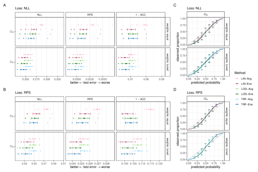
Figure E1: Performance estimates (A, B) and calibration plots (C, D) for the CI_B model fitted on the MNIST data set. The classical linear (LIN-Ens), classical log-linear (LOG-Ens), and transformation (TRF-Ens) ensemble test error is shown for negative log-likelihood (NLL), ranked probability score (RPS) and classification error ($1-\operatorname{ACC}$) in A and B along with the average (AVG) performance measures of the individual members. The average ensemble test error and 95% bootstrap confidence intervals are depicted for six random splits of the data (indicated by different symbols). C and D show calibration and 95% confidence intervals averaged across outcome classes and splits. The predicted probabilities were split at the 0.5, 0.95 quantiles and nine equidistant cut points in-between to calculate the observed event rate in each bin (for details, see Appendix B). In the upper panels ensemble members were equally weighted for constructing the ensemble and in the lower panels weights were tuned to minimize validation loss. In case of equal weights, the average coincides for all ensemble types (LIN-Avg). Models were trained by minimizing NLL (A, C) or RPS (B, D). Note the different scales for A and B.

When additionally tuning the ensemble weights on the validation set, test prediction and discrimination performance improve further. The between-split variation in performance is lower for the weighted ensembles than in ensembles where each member has the same weight, especially when the models were trained by minimizing the NLL (compare upper and lower panels of Fig. E1). For each metric, transformation ensembles perform at least on-par with classical (LIN-Ens and LOG-Ens) ensemble approaches. In this complex intercept model without interpretable additive components, no interpretability is gained when using the transformation instead of the linear or log-linear ensemble.

Note that even though the outcome is nominal, the arbitrarily chosen ordering of the outcome does not influence performance when training with the NLL loss. However, when training the models using the RPS loss which explicitly uses the ordering of the outcome performance is worse in all proper scores and discrimination metrics compared to the models trained by minimizing the NLL (cf. Fig. E1A and B).

The calibration plots (Fig. E1B and D) show a tendency for overconfident predictions. Calibration was slightly better when minimizing NLL instead of RPS during training. No pronounced difference in calibration was observed between single models and ensembles, between types of ensembles or between equal and tuned ensemble weights. Calibration-in-the-large and calibration slope estimates are shown in Appendix E.

Additional results for the MNIST data set

Fig. E2 shows the performance of all $5\times 6$ individual models. Conclusions from the main text remain unaltered. Calibration metrics are summarized in Fig. E3, and again show the slight miscalibration of all models, with worse calibration when using the RPS loss.

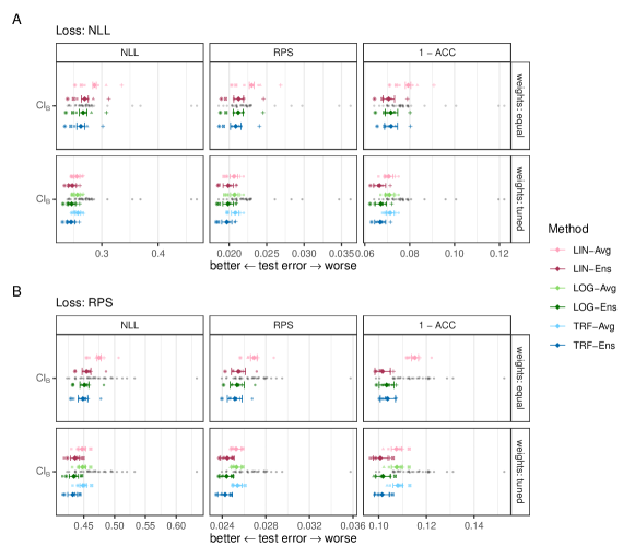
Figure E2: Performance estimates on the MNIST data set. Estimates of individual models are shown as gray dots.

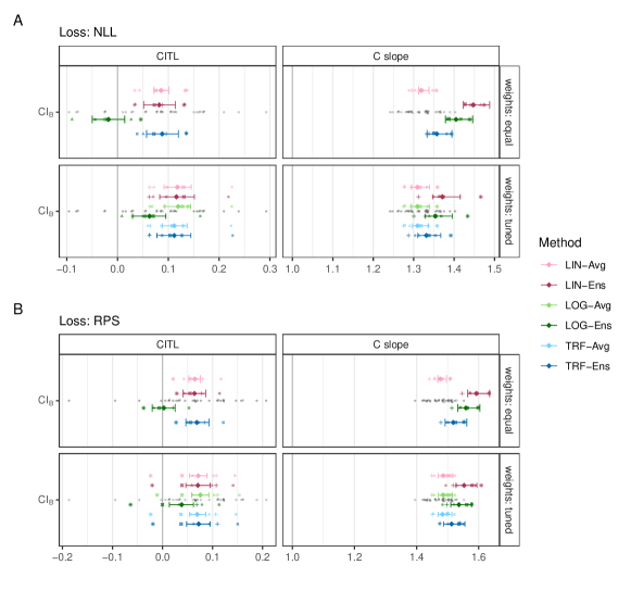
Figure E3: Calibration estimates on the MNIST data set. Calibration-in-the-large (CITL) and calibration slope (C slope) of the classical linear (LIN-Ens), classical log-linear (LOG-Ens), and transformation (TRF-Ens) ensemble.

E.2 Melanoma

Fig. E4 shows model performance relative to the SI-LS${}_{\text{\boldmath$x$}}$ model. Conclusions from the main text remain unaltered; even when removing the between-split variation, variance reduces upon tuning ensemble weights. Performance of individual models is again shown in Fig. E5, and calibration metrics in Fig. E6. Conclusions from the main text remain the same. However, how the extreme miscalibration of some members is mitigated by ensembling can now be seen more clearly.

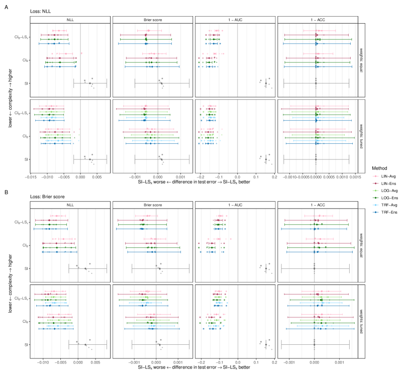
Figure E4: Difference in test error of all models fitted on the melanoma data to the test error of the benchmark SI-LS${}_{\text{\boldmath$x$}}$ model.

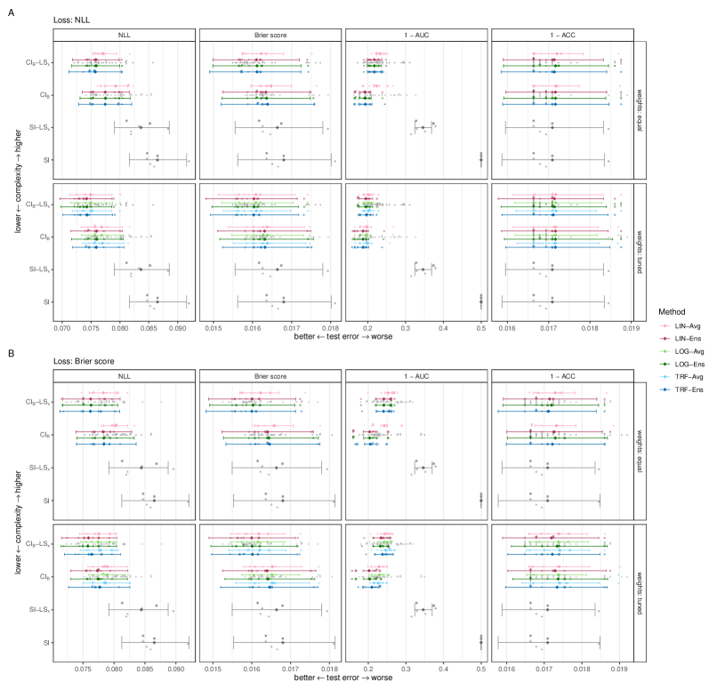
Figure E5: Performance estimates on the melanoma data set. Performance estimates of individual models are shown as gray dots.

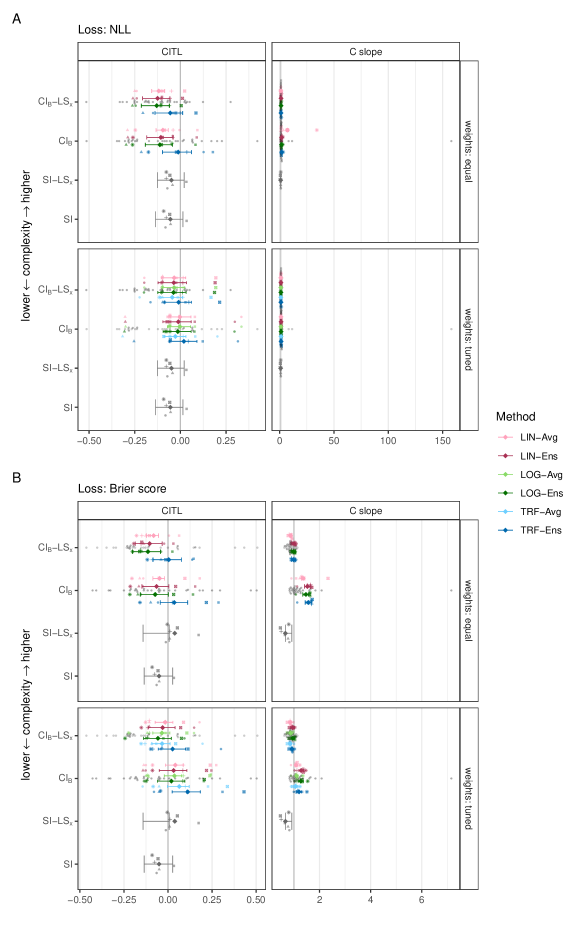
Figure E6: Calibration estimates on the melanoma data set. Calibration-in-the-large (CITL) and calibration slope (C slope) of the classical linear (LIN-Ens), classical log-linear (LOG-Ens), and transformation (TRF-Ens) ensemble. Estimates of individual models are shown as gray dots.

E.3 UTKFace

Fig. E7 shows model performance relative to the SI-LS${}_{\text{\boldmath$x$}}$ model. Conclusions from the main text remain unaltered; even when removing the between-split variation, variance reduces slightly upon tuning ensemble weights. Performance of individual models is again shown in Fig. E8, and calibration metrics in Fig. E9. Ensembles of the CI_B model mitigate stark prediction errors in the individual models. Calibration is better for the CI_B and CI_B-LS${}_{\text{\boldmath$x$}}$ models, the classical log-linear ensemble yields the most well-calibrated predictions for those.

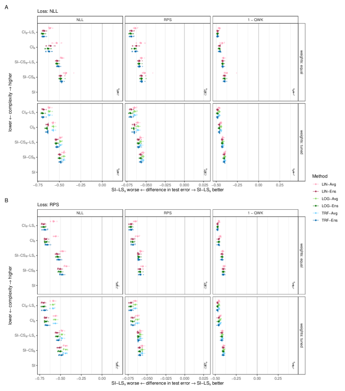
Figure E7: Difference in test error of all models fitted on the UTKFace data to the test error of the benchmark SI-LS${}_{\text{\boldmath$x$}}$ model.

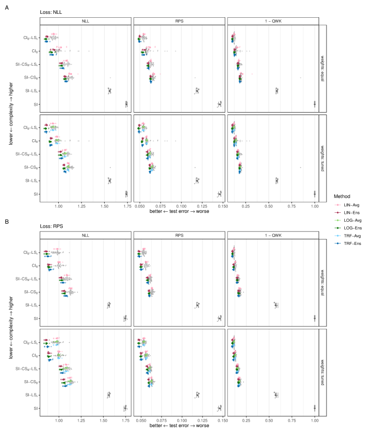
Figure E8: Performance estimates on the UTKFace data set. Estimates of individual models are shown as gray dots.

Figure E9: Calibration estimates on the UTKFace data set. Calibration-in-the-large (CITL) and calibration slope (C slope) of the classical linear (LIN-Ens), classical log-linear (LOG-Ens), and transformation (TRF-Ens) ensemble. Metrics of individual models are shown as gray dots.

References

- Abe et al. [2022] Taiga Abe, E Kelly Buchanan, Geoff Pleiss, Richard Zemel, and John P Cunningham. Deep ensembles work, but are they necessary? arXiv preprint arXiv:2202.06985, 2022. URL http://arxiv.org/abs/2202.06985.
- Allaire and Chollet [2021] JJ Allaire and François Chollet. keras: R Interface to ‘Keras’, 2021. URL https://CRAN.R-project.org/package=keras. R package version 2.7.0.
- Allaire and Tang [2021] JJ Allaire and Yuan Tang. tensorflow: R Interface to ‘TensorFlow’, 2021. URL https://CRAN.R-project.org/package=tensorflow. R package version 2.7.0.
- Baumann et al. [2021] Philipp F. M. Baumann, Torsten Hothorn, and David Rügamer. Deep conditional transformation models. In Machine Learning and Knowledge Discovery in Databases. Research Track, pages 3–18. Springer International Publishing, 2021. doi: 10.1007/978-3-030-86523-8_1.
- Bell [1964] Charles B Bell. A characterization of multisample distribution-free statistics. The Annals of Mathematical Statistics, 35(2):735–738, 1964. doi: 10.1214/aoms/1177703571.
- Berrisch and Ziel [2021] Jonathan Berrisch and Florian Ziel. CRPS learning. Journal of Econometrics, 2021. doi: 10.1016/j.jeconom.2021.11.008.
- Breiman [1996a] Leo Breiman. Bagging predictors. Machine Learning, 24(2):123–140, 1996a. doi: 10.1007/BF00058655.
- Breiman [1996b] Leo Breiman. Stacked regressions. Machine learning, 24(1):49–64, 1996b. doi: 10.1007/BF00117832.
- Breiman [2001a] Leo Breiman. Random forests. Machine Learning, 45(1):5–32, 2001a. doi: 10.1023/A:1010933404324.
- Breiman [2001b] Leo Breiman. Statistical modeling: The two cultures. Statistical Science, 16(3):199–231, 2001b. doi: 10.1214/ss/1009213726.
- Brier [1950] Glenn W Brier. Verification of forecasts expressed in terms of probability. Monthly weather review, 78(1):1–3, 1950. doi: https://doi.org/10.1175/1520-0493(1950)078%3C0001:VOFEIT%3E2.0.CO;2.
- Bröcker [2009] Jochen Bröcker. Reliability, sufficiency, and the decomposition of proper scores. Quarterly Journal of the Royal Meteorological Society, 135(643):1512–1519, 2009. doi: 10.1002/qj.456.
- Bröcker and Smith [2007] Jochen Bröcker and Leonard A Smith. Scoring probabilistic forecasts: The importance of being proper. Weather and Forecasting, 22(2):382–388, 2007. doi: 10.1175/WAF966.1.
- Bühlmann [2012] Peter Bühlmann. Bagging, boosting and ensemble methods. In Handbook of computational statistics, pages 985–1022. Springer, 2012. doi: 10.1007/978-3-642-21551-3_33.
- Cox [1972] D. R. Cox. Regression Models and Life-Tables. Journal of the Royal Statistical Society: Series B (Methodological), 34(2):187–202, 1972. doi: 10.1111/j.2517-6161.1972.tb00899.x.
- Das et al. [2018] Abhijit Das, Antitza Dantcheva, and Francois Bremond. Mitigating bias in gender, age and ethnicity classification: a multi-task convolution neural network approach. ECCVW 2018 - European Conference of Computer Vision Workshops, 2018. doi: 10.1007/978-3-030-11009-3_35.
- Epstein [1969] Edward S Epstein. A scoring system for probability forecasts of ranked categories. Journal of Applied Meteorology (1962-1982), 8(6):985–987, 1969. doi: https://doi.org/10.1175/1520-0450(1969)008%3C0985:ASSFPF%3E2.0.CO;2.
- Fisher [1922] Ronald A Fisher. On the mathematical foundations of theoretical statistics. Philosophical transactions of the Royal Society of London. Series A, containing papers of a mathematical or physical character, 222(594-604):309–368, 1922. doi: 10.1098/rsta.1922.0009.
- Fort et al. [2019] Stanislav Fort, Huiyi Hu, and Balaji Lakshminarayanan. Deep ensembles: A loss landscape perspective. arXiv preprint, 2019. URL http://arXiv.org/abs/1912.02757.
- Gneiting and Raftery [2007] Tilmann Gneiting and Adrian E Raftery. Strictly proper scoring rules, prediction, and estimation. Journal of the American Statistical Association, 102(477):359–378, 2007. doi: 10.1198/016214506000001437.
- Gneiting et al. [2005] Tilmann Gneiting, Adrian E Raftery, Anton H Westveld III, and Tom Goldman. Calibrated probabilistic forecasting using ensemble model output statistics and minimum crps estimation. Monthly Weather Review, 133(5):1098–1118, 2005. doi: 10.1175/MWR2904.1.
- Good [1952] I. J. Good. Rational decisions. Journal of the Royal Statistical Society. Series B (Methodological), 14(1):107–114, 1952. doi: 10.1111/j.2517-6161.1952.tb00104.x.
- Gumbel [1958] Emil Julius Gumbel. Statistics of extremes. Columbia university press, 1958.
- Hansen and Salamon [1990] Lars Kai Hansen and Peter Salamon. Neural network ensembles. IEEE transactions on pattern analysis and machine intelligence, 12(10):993–1001, 1990. doi: 10.1109/34.58871.
- Hoffmann and Elster [2021] Lara Hoffmann and Clemens Elster. Deep ensembles from a bayesian perspective. arXiv preprint arXiv:2105.13283, 2021. URL https://arXiv.org/abs/2105.13283.
- Hothorn [2020] Torsten Hothorn. tram: Transformation Models, 2020. URL https://CRAN.R-project.org/package=tram. R package version 0.5-1.
- Hothorn et al. [2014] Torsten Hothorn, Thomas Kneib, and Peter Bühlmann. Conditional transformation models. Journal of the Royal Statistical Society. Series B: Statistical Methodology, 76(1):3–27, 2014. doi: 10.1111/rssb.12017.
- Hothorn et al. [2018] Torsten Hothorn, Lisa Möst, and Peter Bühlmann. Most Likely Transformations. Scandinavian Journal of Statistics, 45(1):110–134, 2018. doi: 10.1111/sjos.12291.
- Huber [2004] Peter J Huber. Robust statistics, volume 523. John Wiley & Sons, 2004.
- International Skin Imaging Collaboration [2020] International Skin Imaging Collaboration. Siim-isic 2020 challenge dataset, 2020. URL https://challenge2020.isic-archive.com/.
- Ishwaran et al. [2008] Hemant Ishwaran, Udaya B Kogalur, Eugene H Blackstone, and Michael S Lauer. Random survival forests. The Annals of Applied Statistics, 2(3):841–860, 2008. doi: 10.1214/08-AOAS169.
- Kingma and Ba [2015] Diederik P. Kingma and Jimmy Lei Ba. Adam: A method for stochastic optimization. In 3rd International Conference on Learning Representations, ICLR 2015 - Conference Track Proceedings. International Conference on Learning Representations, ICLR, 2015. URL https://arxiv.org/abs/1412.6980v9.
- Kook et al. [2022] Lucas Kook, Lisa Herzog, Torsten Hothorn, Oliver Dürr, and Beate Sick. Deep and interpretable regression models for ordinal outcomes. Pattern Recognition, 122:108263, 2022. doi: 10.1016/j.patcog.2021.108263.
- Kuhn [2022] Max Kuhn. caret: Classification and Regression Training, 2022. URL https://CRAN.R-project.org/package=caret. R package version 6.0-92.
- Lakshminarayanan et al. [2017] Balaji Lakshminarayanan, Alexander Pritzel, and Charles Blundell. Simple and scalable predictive uncertainty estimation using deep ensembles. In Advances in Neural Information Processing Systems, volume 30. Curran Associates, Inc., 2017. URL https://proceedings.neurips.cc/paper/2017/file/9ef2ed4b7fd2c810847ffa5fa85bce38-Paper.pdf.
- LeCun et al. [2010] Yann LeCun, Corinna Cortes, and CJ Burges. Mnist handwritten digit database, 2010. URL http://yann.lecun.com/exdb/mnist. AT&T Labs.
- Molnar [2020] Christoph Molnar. Interpretable machine learning. Lulu.com, 2020.