jTrans: Jump-Aware Transformer for Binary Code Similarity Detection

Abstract.

Binary code similarity detection (BCSD) has important applications in various fields such as vulnerabilities detection, software component analysis, and reverse engineering. Recent studies have shown that deep neural networks (DNNs) can comprehend instructions or control-flow graphs (CFG) of binary code and support BCSD. In this study, we propose a novel Transformer-based approach, namely jTrans, to learn representations of binary code. It is the first solution that embeds control flow information of binary code into Transformer-based language models, by using a novel jump-aware representation of the analyzed binaries and a newly-designed pre-training task. Additionally, we release to the community a newly-created large dataset of binaries, BinaryCorp, which is the most diverse to date. Evaluation results show that jTrans outperforms state-of-the-art (SOTA) approaches on this more challenging dataset by 30.5% (i.e., from 32.0% to 62.5%). In a real-world task of known vulnerability searching, jTrans achieves a recall that is 2X higher than existing SOTA baselines.

1. Introduction

Binary code similarity detection (BCSD), which can identify the degree of similarity between two binary code snippets, is a fundamental technique useful for a wide range of applications, including known vulnerabilities discovery (David and Yahav, 2014; Pewny et al., 2014, 2015; Eschweiler et al., 2016; David et al., 2016; Feng et al., 2016; Huang et al., 2017; Feng et al., 2017; David et al., 2017; Gao et al., 2018; Xu et al., 2017b; David et al., 2018; Shirani et al., 2018; Liu et al., 2018), malware detection (Cesare et al., 2013) and clustering (Hu et al., 2009, 2013; Kim et al., 2019), detection of software plagiarism (Sæbjørnsen et al., 2009; Luo et al., 2014, 2017), patch analysis (Hu et al., 2016; Xu et al., 2017a; Kargén and Shahmehri, 2017), and software supply chain analysis (Hemel et al., 2011). Given the continuously expanding number of binary programs and the fact that binary analysis tasks are widespread, there is a clear need to develop BCSD solutions that are both more scalable and accurate.

Prior to the use of machine learning in the field, traditional BCSD solutions heavily relied on specific features of binary code, i.e., control flow graphs (CFGs) of functions, which capture the syntactic knowledge of programs. Solutions such as BinDiff (zynamics, 2018), BinHunt (Gao et al., 2008) and iBinHunt (Ming et al., 2012) employ graph-isomorphism techniques to calculate the similarity of two functions’ CFGs. This approach, however, is both time-consuming and volatile, since CFGs may change based on compiler optimizations. Studies such as BinGo (Chandramohan et al., 2016) and Esh (David et al., 2016) achieve greater robustness to CFG changes by computing the similarities of CFG fragments. However, these approaches are based on manually crafted features, which have difficulty capturing the precise semantics of binary code. As a result, these solutions tend to have relatively low accuracy.

With the rapid development of machine learning techniques, most current state-of-the-art (SOTA) BCSD solutions are learning-based. In general, these solutions embed target binary code (e.g., functions) into vectors, and compute functions’ similarity in the vector space. Some solutions, e.g., Asm2Vec (Ding et al., 2019) and SAFE (Massarelli et al., 2019a), model assembly language (of machine code) using language models inspired by natural language processing (NLP). Other studies use graph neural networks (GNNs) to learn the representation of CFGs and calculate their similarity (Xu et al., 2017b). Some studies combine both approaches, and learn representations of basic blocks by NLP techniques and further process basic block features in a CFG by GNN, e.g.,  (Yu et al., 2020; Massarelli et al., 2019b). Despite their improved performance, existing methods have several limitations.

First, NLP-based modeling of assembly language only considers the sequential order of instructions and the relationships among them; information regarding the program’s actual execution (e.g., control flows) is not considered. As a result, methods that rely solely on NLP will lack semantic understanding of the analyzed binaries, and will also not be adapt well to possibly significant changes in the code which are the result of compiler optimization.

Secondly, relying solely on CFGs misses semantics of instructions in each basic block. Genius (Feng et al., 2016) and Gemini (Xu et al., 2017b) propose to expand the CFG with manually extracted features (e.g., number of instructions). However, such features are still insufficient to fully capture the code semantics. Furthermore, these solutions generally use GNN to process CFGs, which only captures the structural information. GNNs are also generally known to be relatively difficult to train and apply in parallel, which limits their real-world application.

Thirdly, the datasets on which existing solutions are trained and evaluated are not sufficiently large and/or diverse. Due to the lack of a common large benchmark, each study creates its own dataset, often from small repositories such as GNUtils, coreutils, and openssl. These small datasets have similar code patterns, and therefore lack diversity, which in turn can lead to over-fitted models and a false impression of high performance. Furthermore, the evaluations of existing solutions often does not reflect real-world use cases. The majority of studies did not conduct experiments on a large pool of candidate functions, which are common in the real world. Under more realistic conditions, the performance of many SOTA solutions drops significantly, as we show in our experimental results in Section 6.

In this paper, we present jTrans, a novel Transformer-based model designed to address the aforementioned problems and support real-world binary similarity detection. We combine NLP models, which capture the semantics of instructions, together with CFGs, which capture the control flow information, to infer the representation of binary code. Since previous work (Yu et al., 2020) has shown that a simple combination of NLP-based and GNN-based features does not yield optimal results, we propose to fuse the control-flow information into the Transformer architecture. To the best of our knowledge, we are the first to do so.

We modify the Transformer to capture control-flow information, by sharing parameters between token embeddings and position embeddings for each jump target of instructions. We first use unsupervised learning tasks to pre-train jTrans to learn the semantics of instructions and control-flow information of binary functions. Next, we fine-tune the pre-trained jTrans to match semantically similar functions. Note that our method is able to combine features from each basic block using language models without relying on GNNs to traverse the corresponding CFG.

In addition to our novel approach, we present a large and diversified dataset, BinaryCorp, extracted from ArchLinux’s official repositories (Archlinux, 2021a) and Arch User Repository (AUR) (Archlinux, 2021b). Our newly-created dataset enables us to mitigate the over-fitting and lack of diversity that characterize existing datasets. We automatically collect all the c/c++ projects from the repositories, which contain the majority of popular open-source softwares, and build them with different compiler optimizations to yield different binaries. To the best of our knowledge, ours is the largest and most diversified binary program dataset for BCSD tasks to date.

We implement a prototype of jTrans and evaluate it on real-world BCSD problems, where we show that jTrans significantly outperforms SOTA solutions, including Gemini(Xu et al., 2017b), SAFE (Massarelli et al., 2019a), Asm2Vec (Ding et al., 2019), GraphEmb (Massarelli et al., 2019b) and OrderMatters (Yu et al., 2020). When using the full-sized BinaryCorp in the task of finding the matching function in pools that have 10,000 functions, which is close to real world scenarios, jTrans ranks the correct matching function the highest similarity score (denoted as Recall@1) with a probability of $62.5\%$ on average, while the best of SOTA solutions only achieves $32.0\%$. For the less realistic (and easier) scenario of pools with 32 functions, our approach outperforms its closest competitor by 10.6% (from $84.3\%$ to $94.9\%$) for the same Recall@1 metric. Furthermore, when evaluated on a real-world vulnerability searching task, jTrans achieves a recall score that is 2X higher than the SOTA baselines.

In summary, our study offers the following contributions:

• We propose a novel jump-aware Transformer-based model, jTrans, which is the first solution to embed control-flow information into Transformer. Our approach is able to learn binary code representations and support real world BCSD. We release the code of jTrans at https://github.com/vul337/jTrans.

• We create a new large-scale, well-formed and diversified dataset, BinaryCorp, for the task of BCSD. To the best of our knowledge, BinaryCorp is the most diverse to date, and it can significantly mitigate the overfitting issues of previous benchmarks.

• We conduct extensive experiments, and show that our model can significantly outperform SOTA approaches.

2. Problem Definition

BCSD is a basic task to calculate the similarity of two binary functions. It can be used in three types of scenarios as discussed in (Haq and Caballero, 2019), including (1) One-to-one (OO), where the similarity score of one source function to one target is returned; (2) One-to-many (OM), where a pool of target functions will be sorted based on their similarity scores to one source function; (3) Many-to-many (MM), where a pool of functions will be divided into groups based on similarity.

Without loss of generality, we focus on OM tasks in this study. Note that, we can reduce OM problems to OO problems by setting the size of target functions to 1. We could also extend OM problems to MM, by taking each function in the pool as the source function and solving multiple OM problems. To make the presentation clear, we give a formal definition of the problems as below:

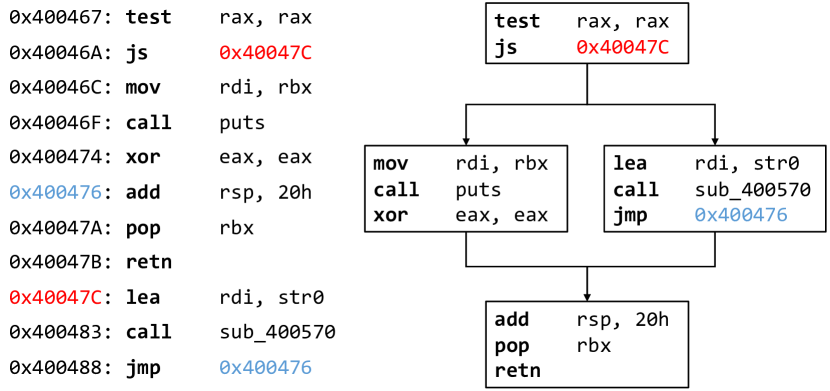
Figure 1. An example control flow of a binary function. The left part is linear layout assembly code with jump addresses, and the right part is the corresponding control-flow graph.

Definition 2.0 (Function).

In this study, we refer a function to a set of ordered instructions in binary programs, which are compiled from a source code function (maybe with inlined functions). It therefore has specific semantics and internal constraints. Especially, a function has a control-flow graph representing its control-flow information, as shown in Figure 1.

The goal of BCSD is developing a solution to calculate the similarity scores of two functions, where two functions compiled from two source code functions that are same or similar to some extent (e.g., one is a patched version of the other) should be similar.

Definition 2.0 (BCSD Task).

Given a source $f_{q}$ and a pool of functions $P$, the binary similarity detection task is to retrieve the top-k functions $\{f_{1},f_{2},\dots,f_{k}|f_{i}\in P\}$ ranked by the similarity score.

3. Related Work

3.1. Non-ML-based BCSD Approaches

Prior to applying machine learning, traditional binary code similarity techniques include static and dynamic methods. Under the assumption that logically similar code shares similar run-time behavior, dynamic analysis methods measure binary code similarity by analyzing manually-crafted dynamic features. This type of solutions includes works such as BinDiff (Dullien and Rolles, 2005), BinHunt (Gao et al., 2008), iBinHunt (Ming et al., 2012), and Genius (Feng et al., 2016), which are based on the CG/CFG graph-isomorphism (GI) Theory (Dullien and Rolles, 2005; Flake, 2004). These works compare the similarity of two binary functions using graph matching algorithms. ESH (David et al., 2016) employs a theorem prover to determine whether two basic blocks are equivalent. This approach, however, is not applicable to the case of different compiler optimizations due to basic block splitting. BinGo (Chandramohan et al., 2016), Blex (Egele et al., 2014) and Multi-MH (Pewny et al., 2015) use randomly sampled values to initialize the context of the function and then compare the similarity by collecting the I/O values. The main shortcoming of these dynamic methods is that they are not suitable for large-scale binary code similarity detection. This is due to the fact that they are computational expensive and require long running time to analyze the whole binary code.

Static methods for BCSD are based on the identification of structural differences in binary code. Methods such as BinClone (Farhadi et al., 2014), ILine (Jang et al., 2013), MutantX-S (Hu et al., 2013), BinSign (Nouh et al., 2017), and Kam1n0 (Ding et al., 2016) use categorized operands or instructions as static features for the computation of binary similarity. Tracelet (David and Yahav, 2014) and BinSequence (Huang et al., 2017) compares the similarity of two binary functions based on the editing distance between instruction sequences. TEDEM (Pewny et al., 2014) and XMATCH (Feng et al., 2017) compute binary similarity using graph/tree edit distance of the basic block expression trees. While static methods are more efficient than dynamic ones, they generally achieve lower accuracy, as they only capture the structural and syntactical information of the binary, and neglect the semantics and relationship between instructions.

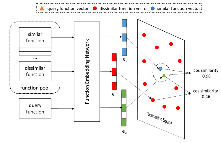
Figure 2. When using embeddings for binary code similarity detection, the query function and candidate functions in function pool are mapped into a semantic vector space. The embeddings of query function, similar function and dissimilar function denote as $e_{q},e_{p}\text{ and }e_{n}$, respectively.

3.2. Learning-based BCSD Approaches

The study of learning-based BCSD has been inspired by recent development in natural language processing (NLP) (Mikolov et al., 2013; Le and Mikolov, 2014; Sutskever et al., 2014), which uses real-valued vectors called embeddings to encode semantic information of words and sentences. Building upon these techniques, previous studies (Xu et al., 2017b; Liu et al., 2018; Gao et al., 2018; Redmond et al., 2018; Zuo et al., 2018; Ding et al., 2019; Massarelli et al., 2019a, b; Yu et al., 2020; Duan et al., 2020; Yang et al., 2021) applied deep learning methods to binary similarity detection. Shared by many of these studies is the idea of embedding binary functions into numerical vectors, and then using vector distance to approximate the similarity between different binary functions. As shown in Figure 2, these methods use deep learning training algorithms to make the vector distances of logically similar binary functions closer.

Most learning-base methods use Siamese network (Chopra et al., 2005), which requires ground-truth mappings of equivalent binary functions to be trained. $\alpha\mathrm{Diff}$ (Liu et al., 2018), for example, learns binary function embeddings directly from the sequence of raw bytes using convolutional neural network (CNN) (Krizhevsky et al., 2012). INNEREYE (Zuo et al., 2018) and RLZ2019 (Redmond et al., 2018) regard instructions as words and basic blocks as sentences, and use word2vec (Mikolov et al., 2013) and LSTM (Hochreiter and Schmidhuber, 1997) to learn basic block embeddings. SAFE (Massarelli et al., 2019a) uses a similar approach to learn the embeddings of binary functions, while Gemini (Xu et al., 2017b), VulSeeker (Gao et al., 2018), GraphEmb (Massarelli et al., 2019b) and OrderMatters (Yu et al., 2020) use GNNs to build a graph embedding model for learning attributed control-flow graph (ACFG) of binary functions. Gemini and VulSeeker encode basic blocks with manually-selected features, while GraphEmb and OrderMatters use neural networks to learn the embeddings of basic blocks. Another approach is propsoed by DEEPBINDIFF (Duan et al., 2020) and Codee (Yang et al., 2021), which uses neural networks to learn the embeddings of generated instruction sequences instead of embedding the ACFG of binary functions.

Unsupervised learning (learing without labels) has also been explored in the field of BCSD. One representative solution is Asm2Vec (Ding et al., 2019). This approach also generates instruction sequences with CFG, but does not rely on the ground truth mappings of equivalent binary functions. Asm2Vec uses an unsupervised algorithm to learn the embedding of binary functions. However, its performance is not as good as the state-of-the-art supervised learning methods.

Overall, learning-based approaches are suitable for large-scale binary code similarity detection, as binary code functions can be transformed into vectors. Then similarity can be computed using vector distance, which is computationally efficient. However, existing techniques have limitations. Some approaches (Xu et al., 2017b; Gao et al., 2018) ignore the semantics of instructions and basic blocks, as they only use manually-selected features to represent basic blocks. Other approaches (Liu et al., 2018; Redmond et al., 2018; Zuo et al., 2018; Massarelli et al., 2019a; Ding et al., 2019; Duan et al., 2020; Yang et al., 2021) neglect some or all of the structural information of binary functions, as they do not use the control-flow information, or generate instruction sequences with CFG using random walk. Finally, methods such as (Massarelli et al., 2019b; Yu et al., 2020) learn basic block embeddings, and use GNN to learn the embedding of attributed control-flow graph (ACFG) of binary functions. While these approaches are effective in some scenarios, they neglect the co-occurrence between inter-basic block instructions.

4. Methodology

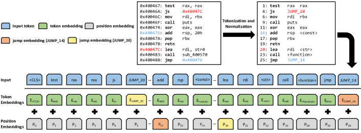
Figure 3. Input representation of jTrans. The raw assembly code is first tokenized and normalized. Then, each token is converted to a token embedding and a position embedding, while its final input embedding is the sum of these two. For each jump pair, its source token’s embedding (e.g., $\mathbf{E_{\mathtt{JUMP\_14}}}$), also called jump embedding, shares parameters with its target token’s position embedding (e.g., $\mathbf{P_{\mathtt{14}}})$.

4.1. Overview

To address the challenge we discussed in Section 1, we propose a novel model, jTrans, for automatically learning the instruction semantics and control-flow information of binary programs. jTrans is based on the Transformer-Encoder architecture (Vaswani et al., 2017), and consists of several significant changes designed to make it more effective for the challenging domain of binary analysis.

The first change we propose to the Transformer architecture is designed to enable jTrans to better capture the code’s jump relationships, i.e., the control-flow information. To this end, we first preprocess the assembly code of the input binary so that it contains the program’s jump relationships. Next, we modify the embedding of the individual input tokens of the Transformer so that the origin and destination locations of the jumps are “semantically” similar.

The second change we propose relates to the training of our proposed model. In view of the similarity between natural language and programs in terms of data flow, we chose to use the commonly used effective Transformer training approach of Masked Language Model (MLM)  (Devlin et al., 2018). MLM-based training requires the model to predict the content of masked tokens based on the content of their neighbors, thus forcing the model to develop a contextual understanding of the relationships among instructions.

Furthermore, to encourage the model to learn the manner by which jumps are incorporated in the code, we propose a novel auxiliary training task that requires the model to predict the target of a jump instruction. This task, which we call Jump Target Prediction (JTP), requires an in-depth understanding of the semantics of the code, and as shown in Section 6.4, it contributes significantly to the performance of our model.

4.2. Binary Function Representation Model

jTrans is based on the BERT architecture (Devlin et al., 2018), which is the state-of-the-art pre-trained language model in many natural language processing (NLP) tasks. In jTrans, we follow the same general approach used by BERT for the modeling of texts, i.e., the creation of an embedding for each token (i.e., word), and the use of BERT’s powerful attention mechanism to effectively model the binary code.

However, binary codes are different from natural languages in several aspects. First, there are way too many vocabularies (e.g., constants and literals) in binary code. Second, there are jump instructions in binary code. For a jump instruction, we denote its operand token as the source token, which specifies the address of the jump target instruction’s address. For simplicity, we denote the mnemonics token of the target instruction as the target token, and represent this jump pair as ¡source token, target token¿.

Therefore, we have to address two problems to apply BERT.

• Out-of-vocabulary (OOV) tokens. As in the field of NLP, we need to train jTrans on a fixed-size vocabulary that contains the most common tokens in the analyzed corpus. Tokens that are not included in the vocabulary need to be represented in a way that enables the Transformer to process them effectively.

• Modeling jump instructions. After preprocessing, the binary code has few information left for the source and target token of a jump pair. BERT can hardly infer the connection between them. This problem is exacerbated by the possible large distance between the source and target, which makes contextual inference even more difficult.

We propose to address these challenges as follows.

4.2.1. Preprocessing instructions.

To mitigate the OOV problem, we use the state-of-the-art disassembly tool IDA Pro 7.5 (Hex-Rays, 2015) to analyze the input binary programs and yield sequences of assembly instructions. We then apply the following tokenization strategies to normalize the assembly code and reduce its vocabulary size:

1. We use the mnemonics and operands as tokens.

2. We replace the string literals with a special token <str>.

3. We replace the constant values with a special token <const>.

4. We keep the external function calls’ names and labels as tokens, and replace the internal function calls’ names as <function>.

5. For each jump pair, we replace its source token (which was absolute or relative address of the jump target) with a token JUMP_XXX, where XXX is the order of the target token of this jump pair, e.g., 20 and 14 in Figure 3. In this way, we can remove the impact of random base addresses of binaries.

4.2.2. Modeling jump instructions.

We now address the challenge of representing jump instructions in a manner that can enable jTrans to better contextualize their bipartite nature (and capture the entire control-flow information as a whole). We chose to use the positional encodings, which are an integral part of the Transformer architecture. These encodings enable the model to determine the distance between tokens. The implicit logic of this representation is that larger distances between tokens generally indicate weaker mutual influence. Jump instructions, however, bind together areas in the code that may be far apart. Therefore we modify the positional encoding mechanism to reflect the effect of jump instructions.

Our changes to the positional encodings are designed to reflect the fact that the source and target of the jump instructions are not only as close as two consecutive tokens (due to order of execution), but also that they have a strong contextual connection. We achieve this goal through parameter sharing: for each jump pair, the source token’s embedding (see $E_{\texttt{JUMP\_14}}$ in Figure 3) is used as the positional encoding of the target token (see $P_{14}$).

This representation achieves two important goals. First, the shared embedding enables the Transformer to identify the contextual connection between the source and target tokens. Secondly, this strong contextual connection is maintained throughout the training process, since the shared parameters are updated for both tokens simultaneously. It is worth noting that we only focus on direct jump instructions in jTrans. We hypothesize that control flow information brought by indirect jumps will further improve the performance of jTrans. However, recognizing targets of such jumps is a well-known open challenge and beyond the scope of our current work. If a solution for recognizing indirect jump targets is proposed in the future, we can embed the operand of the indirect jump with the fusion of the positional embeddings of all jump targets.

4.2.3. The Rationale of Our Proposed Approach

By sharing the parameters between the source and target tokens of the jump pair, we create a high degree of similarity in their representation. As a result, whenever the attention mechanisms that power jTrans assign a high attention weight to one of these tokens (i.e., determine that it is important to the understanding/analysis of the binary), they will automatically also assign high attention to their partner. This representation therefore ensures that both parts of the jump instruction—and the instructions near them in the code—will be included in the inference process.

We now provide a formal analysis of the jump pair’s token similarity, and demonstrate that the similarity within this pair is higher than any of them has with any other token. For a given binary function $\mathbf{f}=[x_{1},\cdots,x_{n}]$, $x_{i}$ is the $i$-th token of $\mathbf{f}$. All the tokens will be converted into mixed embedding vectors $\{E(x_{1}),\cdots,E(x_{n})\}$ before being fed into jTrans, where each embedding $E(x_{i})$ can be represented as a summation of token embeddings $E_{x_{i}}$ and position embeddings $P_{i}$. We apply the multi-head self-attention mechanism (Vaswani et al., 2017) to the mixed embedding vectors $\{E(x_{1}),\cdots,E(x_{n})\}$. We denote the embedding of the $m$-th layer as $E_{m}=[E_{m}(x_{1}),\cdots,E_{m}(x_{n})]$, we first project the $m$-th embedding to $Q_{m}$, $K_{m}$ and $V_{m}$, respectively. Then we used the scaled dot-product attention to get the attention matrix $\text{Attention}(Q_{m},K_{m},V_{m})$.

(1) $$Q_{m}=E_{m}\times W^{Q}_{m},K_{m}=E_{m}\times W^{K}_{m},V_{m}=E_{m}\times W^{V}_{m}$$

$$\text{Attention}(Q_{m},K_{m},V_{m})=\text{Softmax}(\frac{Q_{m}K^{T}_{m}}{\sqrt{d_{k}}})\cdot V_{m}$$

The $W^{Q}_{m}\in\mathbb{R}^{d_{\text{model}}\times d_{k}}$, $W^{K}_{m}\in\mathbb{R}^{d_{\text{model}}\times d_{k}}$, $W^{V}_{m}\in\mathbb{R}^{d_{\text{model}}\times d_{k}}$ are affine transformation matrices of the $m$-th layer, $d_{\text{model}}$ is the dimension of the embedding vector. $\text{Softmax}(\frac{Q_{m}K^{T}_{m}}{\sqrt{d_{k}}})$ is the attention weight matrix. We denote the updated embedding by head $h$ as

(2) $$E^{h}_{m+1}=\text{Attention}(Q^{h}_{m},K^{h}_{m},V^{h}_{m})$$

Assume we have $H$ attention head, we get updated embedding $E_{m+1}$ as follows, $W^{O}_{m}\in\mathbb{R}^{d_{k}H\times d_{\text{model}}}$ is the output transformation matrix of the $m$-th layer, $FFN_{m}$ is the feed-forward network of the $m$-th layer.

(3) $$E_{m+1}=FFN_{m}(\text{Concat}(E^{1}_{m},\cdots,E^{H}_{m})\times W^{O}_{m})$$

The final output of jTrans is the last layer of the model. We produce the function embedding $E_{f}$ as follows, where $W^{F}\in\mathcal{R}^{d_{\text{model}}\times d_{f}}$ is the output transformation matrix, $d_{f}$ is the dimension of the function embedding, $E_{N}(C)$ represents the embedding of <CLS>.

(4) $$E_{f}=tanh(E_{N}(C))\cdot W^{F}$$

Next, we present how jTrans deliver the control-flow information of the program. Consider three tokens $i$, $j$, $l$ in the given function, the corresponding embeddings are $E_{i}$, $E_{j}$ and $E_{l}$. Assume we have a jump relationship between $i$ and $j$, $i$ is the source token and $j$ is the target token. And $l$ is any other token in the function. Denote the attention weight of token $i$ to token $j$ as $A_{ij}=\frac{Q_{i}K_{j}^{T}}{\sqrt{d_{k}}}$. We prove that the mathematical expectation of $A_{ij}$ minus $A_{il}$ is positive. Which can be formulated as follows

(5) $$\small\mathbb{E}[A_{ij}-A_{il}]>0$$

This equation shows that $i$ generally pays more attention to $j$ than $l$. This is the internal explanation of jump embeddings. The detailed proof is in Appendix Appendix.

4.3. Pre-training jTrans

The BERT architecture, on which jTrans is based, uses two unsupervised learning tasks for pre-training. The first task is masked language models (MLM), where BERT is tasked with reconstructing randomly-masked tokens. The second unsupervised learning task is designed to hone BERT’s contextual capabilities by requiring it to determine whether two sentences are consecutive. We build upon BERT’s overall training process, while performing domain-specific adaptations: we preserve the MLM task, but replace the second task with one we call jump task prediction (JTP). As shown in Section 4.3.2, the goal of the JTP task is to improve jTrans’s contextual understanding of jump instructions.

4.3.1. The Masked Language Model Task

Our MLM task closely follows the one proposed in (Devlin et al., 2018), and jTrans uses BERT’s masking procedures: 80% of our randomly-selected tokens are replaced by the mask token (indicating that they need to be reconstructed), 10% are replaced by other random tokens, and 10% are unchanged. Following the notation in Section 4.2.3, we define the function $\mathbf{f}=[x_{1},\cdots,x_{n}]$, where $x_{i}$ is the $i$-th token of $\mathbf{f}$, and $n$ is the number of tokens. We first select a random set of positions for $\mathbf{f}$ to mask out (i.e., $\mathbf{m^{x}}$).

(6) $$\mathbf{f}^{\text{mlm}}=\text{REPLACE}(\mathbf{f},\mathbf{m^{x}},\texttt{<MASK>})$$

Based on these definitions, the MLM objective of reconstructing the masked tokens can be formulated as follows:

(7) $$\small\min_{\theta}\mathcal{L}_{MLM}(\theta)=\sum_{i\in\mathbf{m_{x}}}-\log P(x_{i}|\mathbf{f}^{\text{mlm}})$$

where $\mathbf{m^{x}}$ contains the indices of the masked tokens.

An example of the masking process is presented in Figure 4. We make the rsp, rdi and call tokens, and task jTrans with reconstructing them. To succeed, our model must learn the basic assembly syntax and its contextual information. Successfully reconstructing the rdi token, for example, requires that the model learns the calling convention of the function, while the rsp token requires an understanding of continuous execution.

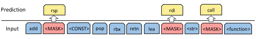
Figure 4. Masked Language Model (MLM)

4.3.2. Jump Target Prediction

The JTP task is defined as follows: given a randomly selected jump source token, our model is required to predict its corresponding target token. This task, which is difficult even for human experts, requires our model to develop a deep understanding of the CFG. This in turn leads to improved performance for jTrans, as we later show in Section 6.4. JTP is carried out by first selecting a random subset of the available jump source tokens. These tokens are then replaced with the token <LOC>.

(8) $$\mathbf{f}^{\text{jtp}}=\text{REPLACE}(\mathbf{f},\mathbf{l^{x}},\texttt{<LOC>})$$

Where $\mathbf{l^{x}}$ is the set of positions for jump symbols. JTP’s objective function can be formulated as follows:

(9) $$\small\min_{\theta}\mathcal{L}_{JTP}(\theta)=\sum_{i\in\mathbf{l_{x}}}-\log P(x_{i}|\mathbf{f}^{\text{jtp}})$$

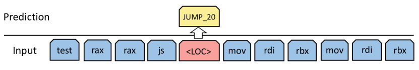
Figure 5. Jump Target Prediction (JTP)

An example of the JTP task is presented in Figure 5, where we replace the JUMP_20 token by <LOC> and the model is tasked with predicting the index. An analysis of jTrans’s performance in the JTP task is presented in Table 6, which shows that our model achieves the accuracy of 92.9%. Furthermore, an ablation study that evaluates JTP’s contribution to jTrans’s overall performance is presented in Section 6.4. These results provide a clear indication that this training task improves jTrans’s ability to learn the control flow of analyzed functions.

The overall loss function of jTrans in the pre-training phase is the summation of the MLM and JTP objective functions:

(10) $$\small\min_{\theta}\mathcal{L}_{P}(\theta)=\mathcal{L}_{MLM}(\theta)+\mathcal{L}_{JTP}(\theta)$$

4.4. Fine-tuning for Binary Similarity Detection

Upon the completion of the unsupervised pre-training phase, we now fine-tune our model for the supervised learning task of function similarity detection. We aim to train jTrans to maximize the similarity between similar binary functions pairs, while minimizing the similarity for unrelated pairs. As shown in Section  4.2.3, we use Equation 4 to represent function $\mathbf{f}$. Our chosen metric for calculating function similarity is Cosine similarity.

We use the following notations: let $\mathcal{F}$ and $\mathcal{G}$ be a set of binary functions, and the sets of similar functions (the “ground truth”). For any query function $\mathbf{f}\in\mathcal{F}$, let $\mathbf{g}^{+}\in\mathcal{G}$ be a function that is similar to $f$ (e.g., compiled from the same source code). Furthermore, let $\mathbf{g}^{-}\in\mathcal{G}$ be an arbitrary function, unrelated to $\mathbf{f}$. We denote the embedding for function $\mathbf{f}$ as $E_{\mathbf{f}}$. Finally, we define $\mathcal{D}$ as the set of all generated triples $\left\langle\mathbf{f},\mathbf{g}^{+},\mathbf{g}^{-}\right\rangle$.

The objective function for our fine-tuning process in trained using contrastive learning (Hadsell et al., 2006; Schroff et al., 2015) and is performed as follows:

(11) $$\small\min_{\theta}\mathcal{L}_{F}(\theta)=\sum_{\langle\mathbf{f},\mathbf{g}^{+},\mathbf{g}^{-}\rangle\in\mathcal{D}}\max\left(0,\varepsilon-\cos\left(E_{\mathbf{f}},E_{\mathbf{g}^{+}}\right)+\cos\left(E_{\mathbf{f}},E_{\mathbf{g}^{-}}\right)\right)$$

where $\theta$ represents the parameters of the model, and $\varepsilon$ is a hyper-parameter usually chosen between 0 and 0.5 (Paszke et al., 2019). After fine-tuning jTrans on $\mathcal{D}$, we can measure the similarity score of two functions $f_{1},f_{2}$ by calculating the cosine similarity of their embeddings. Once the fine-tuning process is complete, we can measure the similarity score of two functions $f_{1},f_{2}$ by calculating the cosine similarity of their embeddings.

4.5. Large-Scale Dataset Construction

We build our dataset for binary similarity detection based on the ArchLinux (Archlinux, 2021a) official repositories and Arch User Repository (Archlinux, 2021b). ArchLinux is a Linux distribution known for its large number of packages and rapid package updates. ArchLinux’s (Archlinux, 2021a) official repositories contain tens of thousands of packages, including editor, instant messenger, HTTP server, web browser, compiler, graphics library, cryptographic library, etc. And Arch User Repository contains more than 77,000 packages uploaded and maintained by users, greatly enlarging the dataset. Furthermore, ArchLinux provides a useful tool makepkg for developers to build their packages from source code. makepkg can compile the specified package from the source by parsing the PKGBUILD file, which contains the required dependencies and compilation helper functions. Binary code similarity task requires a large number of labeled data, thus we use these infrastructures to construct our dataset.

4.5.1. Projects Filtering

For compilation compatibility reasons, we choose the c/c++ project in the pipeline to build the datasets. If the build function in PKGBUILD file contains the call of cmake, make, gcc and g++, then it is very likely to be a C/C++ project. On the other hand, if the variable depend in PKGBUILD file contains rustc, go, jvm, then it is not likely to be a C/C++ project, we can remove it before compiling.

4.5.2. Compilation pipeline

In our pipeline, we wish to automatically specify any optimization level we want each time. The toolchain of some projects do not consume environment variables CFLAGS and CXXFLAGS, making it impossible to change the optimization level easily. However, because most projects call the compiler by CC or CXX, we assign environment variables a self-modified version of gcc, g++, clang, clang++. The modified compiler changes the command line parameters that are related to the optimization level to expected compilation parameters. Also, it appends the expected compilation arguments to the original parameters. We use these two ways to ensure the compilation is done with the expected optimization level.

4.5.3. Label Collection

To collect labels, we need to first obtain unstripped binary and get the offset of functions. We found that many real-world projects call strip during compilation, therefore only specifying parameters in PKGBUILD doesn’t solve this problem. We replaced the strip with its modified version. It will not strip the symbol table regardless of passed-in parameters.

5. Experimental Setup

Table 1. Statistics on the number of projects, binaries and functions of the datasets. Project refers to binaries compiled from the same source code.

Datasets	# Projects	# Binaries	# Functions
GNUtils	20	100	161,202
Coreutils	115	575	76,174
BinaryCorp-3M Train	1,612	8,357	3,126,367
BinaryCorp-3M Test	364	1,908	444,574
BinaryCorp-26M Train	7,845	38,455	21,085,338
BinaryCorp-26M Test	1,974	9,675	4,791,673

5.1. The BinaryCorp Dataset

We now present BinaryCorp, the dataset we created to evaluate large-scale binary similarity detection. BinaryCorp consists of a large number of binaries produced by automatic compilation pipeline, where—based on the official ArchLinux packages and Arch User Repository—we use gcc and g++ to compile 48,130 binary programs with different optimization levels and follow the approach proposed in SAFE(Massarelli et al., 2019a) to filter duplicate functions.

The statistics of our datasets are shown in Table 1. While many previous works use Coreutils and GNUtils as their dataset, Table 1 clearly shows that BinaryCorp-26M operates at a different scale: while our newly-created dataset has approximately 26 million functions compared to GNUtils’ 161,202 and Coreutils 76,174. BinaryCorp-26M is therefore more than 160 times the size of GNUtils and more than 339 the size of Coreutils.

The size of our new dataset prevents the use of some of the existing methods, due to their insufficient scalability. We therefore also provide a smaller dataset, named BinaryCorp-3M, which contains 10,265 binary programs and about 3.6 million functions. The number of functions in our smaller dataset is about 22 times that of GNUtils, and 47 times that of Coreutils.

BinKit(Kim et al., 2020) is the largest binary dataset, which consists 36,256,322 functions. However, BinKit used 1,352 different compile options to generate 243k binaries from only 51 GNU packages, therefore having too many similar functions in the dataset. We, on the other hand, only use 5 different compile options to compile nearly 10,000 projects. While our number of binaries is smaller, our dataset is more diversified than BinKit, in terms of developers, project size, coding style and application scenarios. We argue that our newly generated dataset offers a more diverse—and therefore more realistic—basis for learning and evaluation. Using our datasets, we can evaluate the scalability and efficacy of jTrans (and the other baselines) on a new and larger scale. As mentioned in our contributions in Section 1, we will make our datasets and trained models available to the community.

5.2. Baselines

We compare jTrans to six top-performing baselines:

Genius (Feng et al., 2016). The baseline is a non-deep learning approach. Genius extracts raw features in the form of an attributed control flow graph and uses locality sensitive hashing (LSH) to generate numeric vectors for vulnerability search. We implemented this baseline based on its official code.

Gemini (Xu et al., 2017b). This baseline extracts manually crafted features for each basic block, and uses GNN to learn the CFG representation of the analyzed function. We implemented this approach based on its official Tensorflow code, and used its default parameter settings throughout our evaluation.

SAFE (Massarelli et al., 2019a). This baseline employs an RNN architecture with attention mechanisms to generate a representation of the analyzed function, it receives the assembly instructions as input. We implemented this baseline based on its official Pytorch code, and default parameter settings.

Asm2Vec (Ding et al., 2019). The method uses random walks on the CFG to sample instruction sequences, and then uses the PV-DM model to jointly learn the embedding of the function and instruction tokens. This approach is not open source, and we therefore used an unofficial implementation . We used its default parameter settings.

GraphEmb (Massarelli et al., 2019b). This baseline uses word2vec (Mikolov et al., 2013) to learn the embeddings of the instruction tokens. Next, it uses a RNN to generate independent embeddings for each basic block, and finally uses structure2vec (Dai et al., 2016) to combine the embeddings and generate representation of the analyzed function. To make this baseline scalable to datasets as large as BinaryCorp-26M, we re-implemented the author’s original Tensorflow source code using Pytorch.

OrderMatters (Yu et al., 2020). This method combines two types of embeddings. The first embedding type uses BERT to create an embedding for each basic block, with all these embeddings then combined using a GNN to generate the final representation. The second type of embeddings is obtained by applying a CNN on the CFG. The two embeddings are then concatenated. This method is not open source, and its online blackbox API can not satisfy the need of this study. We implemented on our own using the reported hyperparameters.

Table 2. Results of different binary similarity detection methods on BinaryCorp-3M (Poolsize=32)

		MRR							Recall@1
Models	O0,O3	O1,O3	O2,O3	O0,Os	O1,Os	O2,Os	Average	O0,O3	O1,O3	O2,O3	O0,Os	O1,Os	O2,Os	Average
Gemini	0.388	0.580	0.750	0.455	0.546	0.614	0.556	0.238	0.457	0.669	0.302	0.414	0.450	0.422
SAFE	0.826	0.917	0.958	0.854	0.927	0.927	0.902	0.729	0.869	0.933	0.766	0.879	0.880	0.843
Asm2Vec	0.479	0.878	0.961	0.536	0.855	0.900	0.768	0.351	0.828	0.942	0.408	0.796	0.863	0.701
GraphEmb	0.602	0.694	0.750	0.632	0.674	0.675	0.671	0.485	0.600	0.678	0.521	0.581	0.584	0.575
OrderMatters-online1	0.542	0.740	0.869	0.638	0.702	0.682	0.695	0.414	0.647	0.822	0.515	0.611	0.593	0.591
OrderMatters	0.601	0.838	0.933	0.701	0.812	0.800	0.777	0.450	0.763	0.905	0.566	0.724	0.715	0.687
Genius	0.377	0.587	0.868	0.437	0.600	0.627	0.583	0.243	0.479	0.830	0.298	0.490	0.526	0.478
jTrans-Zero2	0.594	0.841	0.962	0.649	0.850	0.891	0.797	0.499	0.803	0.945	0.566	0.808	0.853	0.746
jTrans	0.947	0.976	0.985	0.956	0.979	0.977	0.970	0.913	0.960	0.974	0.927	0.964	0.961	0.949

• We evaluate OrderMatters with the API provided at https://github.com/binaryai/sdk.

• jTrans-Zero represents jTrans without fine-tuning.

Table 3. Results of different binary similarity detection methods on BinaryCorp-3M (Poolsize=10000)

		MRR							Recall@1
Models	O0,O3	O1,O3	O2,O3	O0,Os	O1,Os	O2,Os	Average	O0,O3	O1,O3	O2,O3	O0,Os	O1,Os	O2,Os	Average
Gemini	0.037	0.161	0.416	0.049	0.133	0.195	0.165	0.024	0.122	0.367	0.030	0.099	0.151	0.132
SAFE	0.127	0.345	0.643	0.147	0.321	0.377	0.320	0.068	0.247	0.575	0.079	0.221	0.283	0.246
Asm2Vec	0.072	0.449	0.669	0.083	0.409	0.510	0.366	0.046	0.367	0.589	0.052	0.332	0.426	0.302
GraphEmb	0.087	0.217	0.486	0.110	0.195	0.222	0.219	0.050	0.154	0.447	0.063	0.135	0.166	0.169
OrderMatters	0.062	0.319	0.600	0.075	0.260	0.233	0.263	0.040	0.248	0.535	0.040	0.178	0.158	0.200
Genius	0.041	0.193	0.596	0.049	0.186	0.224	0.214	0.028	0.153	0.538	0.032	0.146	0.180	0.179
jTrans-Zero	0.137	0.490	0.693	0.182	0.472	0.510	0.414	0.088	0.412	0.622	0.122	0.393	0.430	0.340
jTrans	0.475	0.663	0.731	0.539	0.665	0.664	0.623	0.376	0.580	0.661	0.443	0.586	0.585	0.571

5.3. Evaluation Metrics

Let there be a binary function pool $\mathcal{F}$, and its ground truth binary function pool $\mathcal{G}$.

(12) $$\mathcal{F}=\{f_{1},f_{2},...,f_{i},...,f_{n}\}$$

$$\mathcal{G}=\{f_{1}^{gt},f_{2}^{gt},...,f^{gt}_{i},...,f_{n}^{gt}\}$$

We denote a query function $f_{i}\in\mathcal{F}$ and its corresponding ground truth function $f^{gt}_{i}\in\mathcal{G}$. In this study we address the binary similarity detection problem, and our goal is therefore to retrieve the top-k functions in function pool $\mathcal{G}$, which have the highest similarity to $f_{i}$. The returned functions are ranked by a similarity score, $Rank_{f^{gt}_{i}}$ which denotes their position in the list of retrieved functions. The indicator function $\mathbb{I}$ is defined as below

(13) $$\small\mathbb{I}(x)=\begin{cases}0,&x=False\\ 1,&x=True\end{cases}$$

The retrieval performance can be evaluated using the following two metrics:

(14) $$\text{Recall}@k=\frac{1}{|\mathcal{F}|}\sum_{f_{i}\in\mathcal{F}}\mathbb{I}(\text{Rank}_{f^{gt}_{i}}\leq k)$$

$$\text{MRR}=\frac{1}{|\mathcal{F}|}\sum_{f_{i}\in\mathcal{F}}\frac{1}{Rank_{f^{gt}_{i}}}$$

6. Evaluation

Our evaluation aims to answer the following questions.

• RQ1: How accurate is jTrans in BCSD tasks compared with other baselines? (§6.1)

• RQ2: How well do jTrans and baselines perform on BCSD tasks of different function pool sizes? (§6.2)

• RQ3: How effective is jTrans at discovering known vulnerability? (§6.3)

• RQ4: How effective is our jump-aware design? (§6.4)

• RQ5: How effective is the pre-training design? (§6.5)

Throughout our experiments, all binary files were initially stripped to prevent information leakage. We used IDA Pro to disassemble and extract the functions from the binary code in all of the experiments, thus ensuring a level playing field. For baselines that didn’t use IDA Pro, we used their default disassemble frameworks for preprocessing, after extracting functions using IDA Pro. All the training and inference were run on a Linux server running Ubuntu 18.04 with Intel Xeon 96 core 3.0GHz CPU including hyperthreading, 768GB RAM and 8 Nvidia A100 GPUs.

6.1. Biniary Similarity Detection Performance

We conduct our evaluation on our two datasets, BinaryCorp-3M and BinaryCorp-26M. Additionally, we use two function pool sizes—32 and 10,000—so that jTrans and the baselines can be evaluated in varying degrees of difficulty. It is important to note that we randomly assign entire projects to either the train or test sets of our experiments, because recent studies (Andriesse et al., 2017) have shown that randomly allocating binaries may result in information leakage.

The results of our experiments are presented in Tables 2–5. jTrans outperforms all the baselines by considerable margins. For poolsize=32 (Tables 2) and 4, jTrans outperforms its closest baseline competitor by 0.07 for the MRR metric, and over 10% for the recall@1 metric. The difference in performance becomes more pronounced when we evaluate the models on the larger pool size of 10,000. For this setup, whose results are presented in Tables 3 and 5, jTrans outperforms its closest competitor by 0.26 for the MRR metric, and over 27% for the recall@1 metric.

The results demonstrate the merits of our proposed approach, which utilizes both the Transformer architecture and a novel approach for the representation and analysis of the CFG. We can significantly outperform multiple SOTA approaches such as SAFE, which uses an RNN and performs a less rigorous analysis of the CFG, and OrderMatters, which uses Transformer but analyzes each block independently.

Another important aspect of the results is greater relative degradation in the performance of the baselines for larger pool sizes. In the next section we explore this subject further.

Table 4. Results of different binary similarity detection methods on BinaryCorp-26M (Poolsize=32)

		MRR							Recall@1
Models	O0,O3	O1,O3	O2,O3	O0,Os	O1,Os	O2,Os	Average	O0,O3	O1,O3	O2,O3	O0,Os	O1,Os	O2,Os	Average
Gemini	0.402	0.643	0.835	0.469	0.564	0.628	0.590	0.263	0.528	0.768	0.322	0.441	0.518	0.473
SAFE	0.856	0.940	0.970	0.874	0.935	0.934	0.918	0.770	0.902	0.951	0.795	0.891	0.891	0.867
Asm2Vec	0.439	0.847	0.958	0.490	0.788	0.849	0.729	0.314	0.789	0.940	0.362	0.716	0.800	0.654
GraphEmb	0.583	0.681	0.741	0.610	0.637	0.639	0.649	0.465	0.586	0.667	0.499	0.541	0.543	0.550
OrderMatters	0.572	0.820	0.932	0.630	0.692	0.771	0.729	0.417	0.740	0.903	0.481	0.692	0.677	0.652
jTrans-Zero	0.632	0.871	0.973	0.687	0.890	0.891	0.824	0.539	0.838	0.961	0.602	0.854	0.853	0.775
jTrans	0.964	0.983	0.989	0.969	0.980	0.980	0.978	0.941	0.970	0.981	0.949	0.964	0.964	0.962

Table 5. Results of different binary similarity detection methods on BinaryCorp-26M (Poolsize=10000)

		MRR							Recall@1
Models	O0,O3	O1,O3	O2,O3	O0,Os	O1,Os	O2,Os	Average	O0,O3	O1,O3	O2,O3	O0,Os	O1,Os	O2,Os	Average
Gemini	0.072	0.189	0.474	0.069	0.147	0.202	0.192	0.058	0.148	0.420	0.051	0.115	0.162	0.159
SAFE	0.198	0.415	0.696	0.197	0.377	0.431	0.386	0.135	0.314	0.634	0.127	0.279	0.343	0.305
Asm2Vec	0.118	0.443	0.703	0.107	0.369	0.480	0.370	0.099	0.376	0.638	0.086	0.307	0.413	0.320
GraphEmb	0.116	0.228	0.498	0.133	0.198	0.224	0.233	0.080	0.171	0.465	0.090	0.145	0.175	0.188
OrderMatters	0.113	0.292	0.682	0.118	0.256	0.295	0.292	0.094	0.222	0.622	0.093	0.195	0.236	0.244
jTrans-Zero	0.215	0.570	0.759	0.233	0.571	0.563	0.485	0.167	0.503	0.701	0.175	0.507	0.500	0.426
jTrans	0.584	0.734	0.792	0.627	0.709	0.710	0.693	0.499	0.668	0.736	0.550	0.648	0.648	0.625

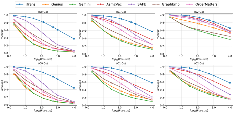
Figure 6. The performance of different binary similarity detection methods on BinaryCorp-3M.

6.2. The Effects of Poolsize on Performance

The results of the previous section highlight the effect of the poolsize variable on the performance of binary similarity detection algorithms. These results are particularly significant given the fact that previous studies use relatively small poolsizes between 10 and 200, with some studies (Xu et al., 2017b; Massarelli et al., 2019a) employing a poolsize of 2. We argue that such setups are problematic, given the fact that for real-world applications such as clone detection and vulnerability search, the poolsize is often larger by orders of magnitude. Therefore, we now present an in-depth analysis of the effects of the poolsize on the performance of SOTA approaches for binary analysis.

The results are presented in Figure 6. We conducted multiple experiments with a variety of poolsizes—2, 10, 32, 128, 512, 1,000, and 10,000—and plotted the results for various optimization pairs. The results clearly show that all baselines’ relative performance is worse than jTrans’s as the poolsize increases. Furthermore, our approach does not display sharp drops in its performance (note that the X-axis in Figure 6 is logarithmic), while the baselines’ performance generally declines more rapidly once poolsize=100 has been reached. This suggests that our approach is not affected so much by the poolsize as it is by the classification problem becoming more challenging due to a large number of candidates.

Finally, we would like to point out that for a very small poolsizes (e.g., 2), the performance of SOTA baselines such as SAFE and Asm2Vec is almost identical to that of jTrans, with the latter outperforming by approximately 2%. We deduce that evaluating binary analysis tools on small poolsizes does not provide meaningful indication to their performance in real-world settings.

6.3. Real-World Vulnerability Search

Vulnerability detection is considered one of the main applications in computer security. We wish to evaluate jTrans’s performance on the real-world task of vulnerability search. In this section, we apply jTrans to a known vulnerabilities dataset with the task of searching for vulnerable functions.

We perform our evaluation on eight CVEs extracted from a known vulnerabilities dataset (SecretPatch, 2021). We produce 10 variants for each function by using different compilers (gcc, clang) and different optimization levels. Our evaluation metric was the recall@10 metric. To simulate real-world settings, we use all of the functions in the project as the search pool. The number of functions for each project varies from 3,038 to 60,159, with the latter being highly challenging.

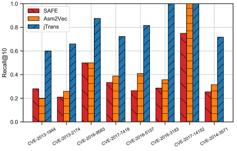
Figure 7. Recall@10 of real-world vulnerability search.

Figure 7 presents the results for the recall@10 metric for each of our queries. We compare our approach to the two leading baselines from Sections 6.1 and 6.2—SAFE and Asm2Vec. It is clear that for most of the CVEs, jTrans’s performance is significantly higher than that of the two baselines. For example, on CVE-2016-3183 from the openjpeg project containing 3,038 functions, our approach achieved a top-10 recall of $100\%$, meaning that it successfully retrieved all the 10 variants, while Asm2Vec and SAFE achieved recall@10 values of $36.9\%$ and $28.6\%$, respectively. Our results demonstrate that jTrans can be effectively deployed as a vulnerability search tool in real-world scenarios, as a result of its ability to perform well on large pool sizes.

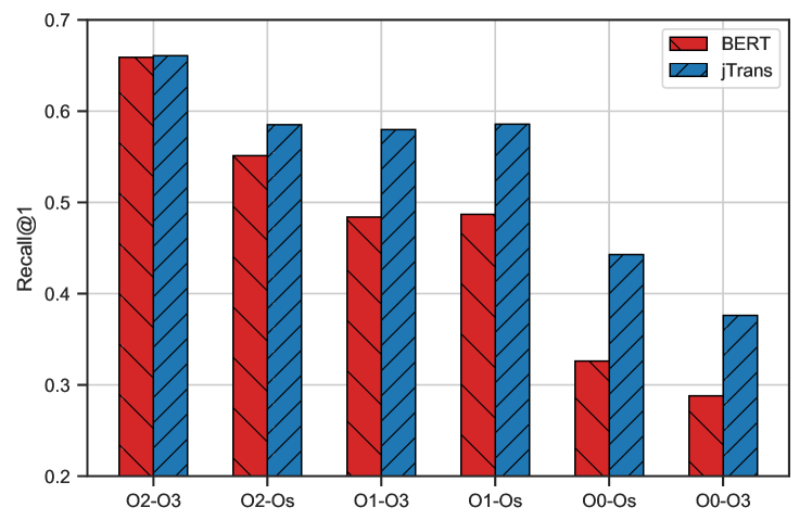
Figure 8. Recall@1 of jTrans and BERT on BinaryCorp-3M when poolsize equals 10,000.

6.4. The Impact of Our Jump-aware Design

In this section, we test our hypothesis that our jump-aware design significantly contributes to jTrans’ ability to analyze the CFG of the binary code. To this end, we train a standard BERT model that does not use our representation of the jump information and compare it to our approach. The hyperparameters used by both models for the pre-training and fine-tuning tasks are identical, with the only distinction being that for BERT we replace the address of each jump token with a fixed token representing an arbitrary address. As a result, similarly to SAFE, the standard BERT does not receive the control flow information, and can only learn from assembly sequence information.

We evaluate the standard BERT model and jTrans on BinaryCorp-3M using Recall@1, with poolsize=10,000. The results of our evaluation are presented in Figure 8. The results clearly show that the standard BERT performs significantly worse than jTrans, as its performance is lower on each optimization pair. On average, jTrans outperforms BERT by $7.3\%$. These results clearly show that incorporating control flow information into the assembly language sequence modeling is highly beneficial for our model.

Table 6. Accuracy of jTrans in Jump Target Prediction (JTP) task on BinaryCorp-3M

	top-1	top-3	top-5	top-10
Accuracy	0.929	0.984	0.991	0.995

To further explore the efficacy of our jump-aware design, we analyze the ability of our pre-trained model to predict the masked jump addresses in the binary code. We conduct our experiment on BinaryCorp-3M. For each function in the evaluation set, we randomly sample some jump positions with 15% probability, and replace them with <LOC> in the function. We then analyze the probability of the model correctly predicting the jump target position for each masked jump target. Our results, presented in Table 6, show that jTrans is highly capable at predicting jump positions. Our pre-trained model can predict the target of the jump instruction with top-1 accuracy of 92.9% and top-10 accuracy of 99.5%. This accuracy is quite high, particularly for top-1, as there are 512 possible jump positions. These results indicate our pre-trained model was able to successfully capture the contextual instruction information of the binary.

6.5. Evaluating the Efficacy of Pre-training

As is the original BERT, pre-training is a critical component of our model. Its main advantage is that it can be performed on unlabeled data, which is much easier to obtain in large quantities. To evaluate the effectiveness of the pre-training approach (MLM and JTP), we evaluated a version of our model that does not perform any fine-tuning. We follow the same approach as in zero-shot learning (Xian et al., 2017), where we use binaries without label information in the pre-training phase. Then, without fine-tuning the pre-trained model, we immediately apply it to the task of binary similarity search. The results of this model, denoted as jTrans-zero, are presented in Tables 2–5.

The results clearly show the efficacy of our pre-training approach. Even without fine-tuning, jTrans-zero outperforms all the baselines for poolsize=10000: on BinaryCorp-26M, compared to the closest baseline, jTrans-zero improves 0.1 for the MRR metric, and improves 10.6% for the recall@1 metric. In the poolsize=32 setup, jTrans-zero outperforms all baselines except SAFE, with latter outperforming our approach by 11.4%. It is important to note, however, that poolsize-32 is far less indicative for real-world scenarios, and in the more challenging poolsize=10000, even our partially-trained approach performed significantly better.

7. Discussion

We focus on training jTrans on one architecture (e.g x86) in this paper, but the technique we proposed can be applied to other architectures as well. jTrans provides a novel solution to binary code similarity detection tasks, outperforming state-of-the-art solutions. It can be applied to many applications, including discovering known vulnerabilities in unknown binaries (David and Yahav, 2014; Pewny et al., 2014, 2015; Eschweiler et al., 2016), malware detection (Cesare et al., 2013) and clustering (Hu et al., 2009), detection of software plagiarism (Sæbjørnsen et al., 2009), patch analysis (Hu et al., 2016; Xu et al., 2017a), and software supply chain analysis (Hemel et al., 2011). For instance, due to the rapid deployment of IoT devices, code reusing is very common in IoT development. BCSD solutions like jTrans could help detect whether IoT devices have vulnerabilities revealed in open source libraries. In the scenario of blockchains, a huge number of blockchains and smart contracts are developed in the past 5 years, based on numerous code cloning and forking. However, the security risks of blockchains and smart contracts are severe, and a large portion of them are vulnerable. The code dependency between different blockchains and smart contracts makes this issue even worse. We could use jTrans to efficiently detect vulnerabilities in blockchains and smart contracts.

Existing deep learning-based works, as well as jTrans, embed individual binary functions into numerical vectors, and compare similarity between vectors. As a result, their accuracy drops along with the pool size. As shown in Figure 6, the accuracy of most existing solutions drops below 20% if the pool size is 10,000. In real world scenarios, the pool size would be much larger. A model that directly takes two binary functions as input could better capture the inter-function relationships and further improve the performance of BCSD, even in a large pool. However, training a model to directly compare two functions would have higher overheads. We leave balancing the accuracy and overhead when using jTrans in real world BCSD tasks as a future work.

8. Conclusion

In this work we propose jTrans, the first solution to embed control-flow information to Transformer-based language models. Our approach utilizes a novel jump-aware architecture design that does not rely on the use of GNNs. Theoretical analysis of self attention shows the soundness of our design. Experimental results demonstrate that our method consistently outperforms state-of-the-art approaches by a large margin on BCSD tasks. Through intensive evaluation, we also uncover weaknesses in the evaluation of current SOTA methods. Additionally, we present and release to the community a newly-created dataset named BinaryCorp. Our dataset contains the largest amount of diversified binaries to date, and we believe that it can be used as a high-quality benchmark for future studies in this field.

Appendix

Proof.

We denote the embedding of the $m$-th layer as $E_{m}$, we first project the $m$-th embedding to $Q_{m}$, $K_{m}$ and $V_{m}$, respectively. Then we used the scaled dot-product attention to get the attention matrix Attention. For notation brevity, we use $E,Q,K,V$ to replace $E_{m},Q_{m},K_{m},V_{m}$, use $q,k,v,d$ to replace $W^{Q}_{m},W^{K}_{m},W^{V}_{m},d_{k}$ in the derivation.

From the embedding projection and attention calculation, we have:

(15) $$Q=E\times q,\quad K=E\times k,\quad V=E\times v$$

$$\text{Attention}(Q,K,V)=\text{Softmax}(\frac{QK^{T}}{\sqrt{d}})\cdot V$$

We denote the attention weight matrix before softmax is $A$:

(16) $$A=\frac{Q\times K^{T}}{\sqrt{d}}=\frac{Eq\times k^{T}E^{T}}{\sqrt{d}}\\$$

Let matrix $J=\frac{q\times k^{T}}{\sqrt{d}}$, then we have:

(17) $$A=EJE^{T}\\$$

(18) $$\forall i,j,A_{i,j}=E_{i}J(E_{j})^{T}=tr(E_{i}J(E_{j})^{T})=tr((E_{j})^{T}E_{i}J)\\$$

We then apply SVD decomposition to matrix $J$, and get $J=U\times S\times V^{T}$, where, $U$ and $V$ are orthogonal, $S=diag(s_{1},s_{2},...,s_{N}),s_{i}\geq 0$.

(19) $$A_{i,j} =tr((E_{j})^{T}E_{i}USV^{T})$$

(20) $$=tr((E_{j})^{T}E_{i}US)$$

(21) $$=tr(S(E_{j})^{T}E_{i}U)$$

(22) $$=tr(S(E_{j})^{T}E_{i})$$

(23) $$=tr(diag(s_{1},s_{2},...,s_{N})(E_{j})^{T}E_{i})$$

(24) $$=\sum_{n=1}^{N}s_{n}E_{in}E_{jn}$$

Similarly, we could get

(25) $$\forall l,A_{il}=\sum_{n=1}^{N}s_{n}E_{in}E_{ln}$$

Therefore we have

(26) $$A_{ij}-A_{il}=\sum_{n=1}^{N}s_{n}E_{in}(E_{jn}-E_{ln})$$

Denote $T$ as token embedding of current layer, $P$ is position embedding of current layer. Assume $E=P+T$. When position $i$ is jump connected with position $j$. $T_{i}=P_{j}$, other embeddings follow a normal distribution

(27) $$T_{i}\sim N(0,\sigma^{2}I),P_{i}\sim N(0,\sigma^{2}I),$$

(28) $$T_{j}\sim N(0,\sigma^{2}I),$$

(29) $$T_{l}\sim N(0,\sigma^{2}I),P_{l}\sim N(0,\sigma^{2}I)$$

We have

(30) $$A_{ij}-A_{il}=\sum_{n=1}^{N}s_{n}(P_{in}+T_{in})(T_{jn}+P_{jn}-T_{ln}-P_{ln})$$

Taking the expectation of this formula,

(31) $$\mathbb{E}(A_{ij}-A_{il}) =\sum_{n=1}^{N}s_{n}\mathbb{E}((P_{in}+T_{in})(T_{jn}+P_{jn}-T_{ln}-P_{ln}))$$

(32) $$=\sum_{n=1}^{N}s_{n}\mathbb{E}(T_{in}P_{jn})$$

(33) $$=\sum_{n=1}^{N}s_{n}\mathbb{E}(T_{in}^{2})$$

(34) $$=\sigma^{2}\sum_{n=1}^{N}s_{n}$$

Therefore we have

(35) $$\mathbb{E}(A_{ij}-A_{il})=\sigma^{2}\sum_{n=1}^{N}s_{n}>0$$

∎

References

- (1)
- Andriesse et al. (2017) Dennis Andriesse, Asia Slowinska, and Herbert Bos. 2017. Compiler-Agnostic Function Detection in Binaries. In 2017 IEEE European Symposium on Security and Privacy (EuroS P). 177–189. https://doi.org/10.1109/EuroSP.2017.11
- Archlinux (2021a) Archlinux. 2021a. Arch linux. Retrieved August 8, 2021 from https://archlinux.org/packages/
- Archlinux (2021b) Archlinux. 2021b. Arch User Repository. Retrieved August 8, 2021 from https://aur.archlinux.org/
- Cesare et al. (2013) Silvio Cesare, Yang Xiang, and Wanlei Zhou. 2013. Control flow-based malware variantdetection. IEEE Transactions on Dependable and Secure Computing 11, 4 (2013), 307–317.
- Chandramohan et al. (2016) Mahinthan Chandramohan, Yinxing Xue, Zhengzi Xu, Yang Liu, Chia Yuan Cho, and Hee Beng Kuan Tan. 2016. Bingo: Cross-architecture cross-os binary search. In Proceedings of the 2016 24th ACM SIGSOFT International Symposium on Foundations of Software Engineering. 678–689.
- Chopra et al. (2005) Sumit Chopra, Raia Hadsell, and Yann LeCun. 2005. Learning a similarity metric discriminatively, with application to face verification. In 2005 IEEE Computer Society Conference on Computer Vision and Pattern Recognition (CVPR’05), Vol. 1. IEEE, 539–546.
- Dai et al. (2016) Hanjun Dai, Bo Dai, and Le Song. 2016. Discriminative embeddings of latent variable models for structured data. In International conference on machine learning. PMLR, 2702–2711.
- David et al. (2016) Yaniv David, Nimrod Partush, and Eran Yahav. 2016. Statistical similarity of binaries. ACM SIGPLAN Notices 51, 6 (2016), 266–280.
- David et al. (2017) Yaniv David, Nimrod Partush, and Eran Yahav. 2017. Similarity of binaries through re-optimization. In Proceedings of the 38th ACM SIGPLAN Conference on Programming Language Design and Implementation. 79–94.
- David et al. (2018) Yaniv David, Nimrod Partush, and Eran Yahav. 2018. Firmup: Precise static detection of common vulnerabilities in firmware. ACM SIGPLAN Notices 53, 2 (2018), 392–404.
- David and Yahav (2014) Yaniv David and Eran Yahav. 2014. Tracelet-based code search in executables. Acm Sigplan Notices 49, 6 (2014), 349–360.
- Devlin et al. (2018) Jacob Devlin, Ming-Wei Chang, Kenton Lee, and Kristina Toutanova. 2018. Bert: Pre-training of deep bidirectional transformers for language understanding. arXiv preprint arXiv:1810.04805 (2018).
- Ding et al. (2016) Steven HH Ding, Benjamin CM Fung, and Philippe Charland. 2016. Kam1n0: Mapreduce-based assembly clone search for reverse engineering. In Proceedings of the 22nd ACM SIGKDD International Conference on Knowledge Discovery and Data Mining. 461–470.
- Ding et al. (2019) Steven HH Ding, Benjamin CM Fung, and Philippe Charland. 2019. Asm2vec: Boosting static representation robustness for binary clone search against code obfuscation and compiler optimization. In 2019 IEEE Symposium on Security and Privacy (SP). IEEE, 472–489.
- Duan et al. (2020) Yue Duan, Xuezixiang Li, Jinghan Wang, and Heng Yin. 2020. Deepbindiff: Learning program-wide code representations for binary diffing. In Network and Distributed System Security Symposium.
- Dullien and Rolles (2005) Thomas Dullien and Rolf Rolles. 2005. Graph-based comparison of executable objects (english version). Sstic 5, 1 (2005), 3.
- Egele et al. (2014) Manuel Egele, Maverick Woo, Peter Chapman, and David Brumley. 2014. Blanket execution: Dynamic similarity testing for program binaries and components. In 23rd USENIX Security Symposium (USENIX Security 14). 303–317.
- Eschweiler et al. (2016) Sebastian Eschweiler, Khaled Yakdan, and Elmar Gerhards-Padilla. 2016. discovRE: Efficient Cross-Architecture Identification of Bugs in Binary Code.. In NDSS, Vol. 52. 58–79.
- Farhadi et al. (2014) Mohammad Reza Farhadi, Benjamin CM Fung, Philippe Charland, and Mourad Debbabi. 2014. Binclone: Detecting code clones in malware. In 2014 Eighth International Conference on Software Security and Reliability (SERE). IEEE, 78–87.
- Feng et al. (2017) Qian Feng, Minghua Wang, Mu Zhang, Rundong Zhou, Andrew Henderson, and Heng Yin. 2017. Extracting conditional formulas for cross-platform bug search. In Proceedings of the 2017 ACM on Asia Conference on Computer and Communications Security. 346–359.
- Feng et al. (2016) Qian Feng, Rundong Zhou, Chengcheng Xu, Yao Cheng, Brian Testa, and Heng Yin. 2016. Scalable graph-based bug search for firmware images. In Proceedings of the 2016 ACM SIGSAC Conference on Computer and Communications Security. 480–491.
- Flake (2004) Halvar Flake. 2004. Structural comparison of executable objects. In Detection of intrusions and malware & vulnerability assessment, GI SIG SIDAR workshop, DIMVA 2004. Gesellschaft für Informatik eV.
- Gao et al. (2008) Debin Gao, Michael K Reiter, and Dawn Song. 2008. Binhunt: Automatically finding semantic differences in binary programs. In International Conference on Information and Communications Security. Springer, 238–255.
- Gao et al. (2018) Jian Gao, Xin Yang, Ying Fu, Yu Jiang, and Jiaguang Sun. 2018. VulSeeker: a semantic learning based vulnerability seeker for cross-platform binary. In 2018 33rd IEEE/ACM International Conference on Automated Software Engineering (ASE). IEEE, 896–899.
- Hadsell et al. (2006) Raia Hadsell, Sumit Chopra, and Yann LeCun. 2006. Dimensionality reduction by learning an invariant mapping. In 2006 IEEE Computer Society Conference on Computer Vision and Pattern Recognition (CVPR’06), Vol. 2. IEEE, 1735–1742.
- Haq and Caballero (2019) Irfan Ul Haq and Juan Caballero. 2019. A survey of binary code similarity. arXiv preprint arXiv:1909.11424 (2019).
- Hemel et al. (2011) Armijn Hemel, Karl Trygve Kalleberg, Rob Vermaas, and Eelco Dolstra. 2011. Finding software license violations through binary code clone detection. In Proceedings of the 8th Working Conference on Mining Software Repositories. 63–72.
- Hex-Rays (2015) Hex-Rays. 2015. IDA Pro Disassembler and Debugger. Retrieved April 10, 2018 from https://www.hex-rays.com/products/ida/index.shtml
- Hochreiter and Schmidhuber (1997) Sepp Hochreiter and Jürgen Schmidhuber. 1997. Long short-term memory. Neural computation 9, 8 (1997), 1735–1780.
- Hu et al. (2009) Xin Hu, Tzi-cker Chiueh, and Kang G Shin. 2009. Large-scale malware indexing using function-call graphs. In Proceedings of the 16th ACM conference on Computer and communications security. 611–620.
- Hu et al. (2013) Xin Hu, Kang G Shin, Sandeep Bhatkar, and Kent Griffin. 2013. Mutantx-s: Scalable malware clustering based on static features. In 2013 USENIX Annual Technical Conference (USENIXATC 13). 187–198.
- Hu et al. (2016) Yikun Hu, Yuanyuan Zhang, Juanru Li, and Dawu Gu. 2016. Cross-architecture binary semantics understanding via similar code comparison. In 2016 IEEE 23rd International Conference on Software Analysis, Evolution, and Reengineering (SANER), Vol. 1. IEEE, 57–67.
- Huang et al. (2017) He Huang, Amr M Youssef, and Mourad Debbabi. 2017. Binsequence: Fast, accurate and scalable binary code reuse detection. In Proceedings of the 2017 ACM on Asia Conference on Computer and Communications Security. 155–166.
- Jang et al. (2013) Jiyong Jang, Maverick Woo, and David Brumley. 2013. Towards automatic software lineage inference. In 22nd USENIX Security Symposium (USENIX Security 13). 81–96.
- Kargén and Shahmehri (2017) Ulf Kargén and Nahid Shahmehri. 2017. Towards robust instruction-level trace alignment of binary code. In 2017 32nd IEEE/ACM International Conference on Automated Software Engineering (ASE). IEEE, 342–352.
- Kim et al. (2020) Dongkwan Kim, Eunsoo Kim, Sang Kil Cha, Sooel Son, and Yongdae Kim. 2020. Revisiting binary code similarity analysis using interpretable feature engineering and lessons learned. arXiv preprint arXiv:2011.10749 (2020).
- Kim et al. (2019) TaeGuen Kim, Yeo Reum Lee, BooJoong Kang, and Eul Gyu Im. 2019. Binary executable file similarity calculation using function matching. The Journal of Supercomputing 75, 2 (2019), 607–622.
- Krizhevsky et al. (2012) Alex Krizhevsky, Ilya Sutskever, and Geoffrey E Hinton. 2012. Imagenet classification with deep convolutional neural networks. Advances in neural information processing systems 25 (2012), 1097–1105.
- Le and Mikolov (2014) Quoc Le and Tomas Mikolov. 2014. Distributed representations of sentences and documents. In International conference on machine learning. PMLR, 1188–1196.
- Liu et al. (2018) Bingchang Liu, Wei Huo, Chao Zhang, Wenchao Li, Feng Li, Aihua Piao, and Wei Zou. 2018. diff: cross-version binary code similarity detection with dnn. In Proceedings of the 33rd ACM/IEEE International Conference on Automated Software Engineering. 667–678.
- Luo et al. (2014) Lannan Luo, Jiang Ming, Dinghao Wu, Peng Liu, and Sencun Zhu. 2014. Semantics-based obfuscation-resilient binary code similarity comparison with applications to software plagiarism detection. In Proceedings of the 22nd ACM SIGSOFT International Symposium on Foundations of Software Engineering. 389–400.
- Luo et al. (2017) Lannan Luo, Jiang Ming, Dinghao Wu, Peng Liu, and Sencun Zhu. 2017. Semantics-based obfuscation-resilient binary code similarity comparison with applications to software and algorithm plagiarism detection. IEEE Transactions on Software Engineering 43, 12 (2017), 1157–1177.
- Massarelli et al. (2019a) Luca Massarelli, Giuseppe Antonio Di Luna, Fabio Petroni, Roberto Baldoni, and Leonardo Querzoni. 2019a. Safe: Self-attentive function embeddings for binary similarity. In International Conference on Detection of Intrusions and Malware, and Vulnerability Assessment. Springer, 309–329.
- Massarelli et al. (2019b) Luca Massarelli, Giuseppe A Di Luna, Fabio Petroni, Leonardo Querzoni, and Roberto Baldoni. 2019b. Investigating graph embedding neural networks with unsupervised features extraction for binary analysis. In Proceedings of the 2nd Workshop on Binary Analysis Research (BAR).
- Mikolov et al. (2013) Tomas Mikolov, Kai Chen, Greg Corrado, and Jeffrey Dean. 2013. Efficient estimation of word representations in vector space. arXiv preprint arXiv:1301.3781 (2013).
- Ming et al. (2012) Jiang Ming, Meng Pan, and Debin Gao. 2012. iBinHunt: Binary hunting with inter-procedural control flow. In International Conference on Information Security and Cryptology. Springer, 92–109.
- Nouh et al. (2017) Lina Nouh, Ashkan Rahimian, Djedjiga Mouheb, Mourad Debbabi, and Aiman Hanna. 2017. BinSign: Fingerprinting binary functions to support automated analysis of code executables. In IFIP International Conference on ICT Systems Security and Privacy Protection. Springer, 341–355.
- Paszke et al. (2019) Adam Paszke, Sam Gross, Francisco Massa, Adam Lerer, James Bradbury, Gregory Chanan, Trevor Killeen, Zeming Lin, Natalia Gimelshein, Luca Antiga, et al. 2019. Pytorch: An imperative style, high-performance deep learning library. Advances in neural information processing systems 32 (2019), 8026–8037.
- Pewny et al. (2015) Jannik Pewny, Behrad Garmany, Robert Gawlik, Christian Rossow, and Thorsten Holz. 2015. Cross-architecture bug search in binary executables. In 2015 IEEE Symposium on Security and Privacy. IEEE, 709–724.
- Pewny et al. (2014) Jannik Pewny, Felix Schuster, Lukas Bernhard, Thorsten Holz, and Christian Rossow. 2014. Leveraging semantic signatures for bug search in binary programs. In Proceedings of the 30th Annual Computer Security Applications Conference. 406–415.
- Redmond et al. (2018) Kimberly Redmond, Lannan Luo, and Qiang Zeng. 2018. A cross-architecture instruction embedding model for natural language processing-inspired binary code analysis. arXiv preprint arXiv:1812.09652 (2018).
- Sæbjørnsen et al. (2009) Andreas Sæbjørnsen, Jeremiah Willcock, Thomas Panas, Daniel Quinlan, and Zhendong Su. 2009. Detecting code clones in binary executables. In Proceedings of the eighteenth international symposium on Software testing and analysis. 117–128.
- Schroff et al. (2015) Florian Schroff, Dmitry Kalenichenko, and James Philbin. 2015. Facenet: A unified embedding for face recognition and clustering. In Proceedings of the IEEE conference on computer vision and pattern recognition. 815–823.
- SecretPatch (2021) SecretPatch. 2021. SecretPatch. Retrieved August 8, 2021 from https://github.com/SecretPatch/Dataset
- Shirani et al. (2018) Paria Shirani, Leo Collard, Basile L Agba, Bernard Lebel, Mourad Debbabi, Lingyu Wang, and Aiman Hanna. 2018. Binarm: Scalable and efficient detection of vulnerabilities in firmware images of intelligent electronic devices. In International Conference on Detection of Intrusions and Malware, and Vulnerability Assessment. Springer, 114–138.
- Sutskever et al. (2014) Ilya Sutskever, Oriol Vinyals, and Quoc V Le. 2014. Sequence to sequence learning with neural networks. In Advances in neural information processing systems. 3104–3112.
- Vaswani et al. (2017) Ashish Vaswani, Noam Shazeer, Niki Parmar, Jakob Uszkoreit, Llion Jones, Aidan N Gomez, Łukasz Kaiser, and Illia Polosukhin. 2017. Attention is all you need. In Advances in neural information processing systems. 5998–6008.
- Xian et al. (2017) Yongqin Xian, Bernt Schiele, and Zeynep Akata. 2017. Zero-shot learning-the good, the bad and the ugly. In Proceedings of the IEEE Conference on Computer Vision and Pattern Recognition. 4582–4591.
- Xu et al. (2017b) Xiaojun Xu, Chang Liu, Qian Feng, Heng Yin, Le Song, and Dawn Song. 2017b. Neural network-based graph embedding for cross-platform binary code similarity detection. In Proceedings of the 2017 ACM SIGSAC Conference on Computer and Communications Security. 363–376.
- Xu et al. (2017a) Zhengzi Xu, Bihuan Chen, Mahinthan Chandramohan, Yang Liu, and Fu Song. 2017a. Spain: security patch analysis for binaries towards understanding the pain and pills. In 2017 IEEE/ACM 39th International Conference on Software Engineering (ICSE). IEEE, 462–472.
- Yang et al. (2021) Jia Yang, Cai Fu, Xiao-Yang Liu, Heng Yin, and Pan Zhou. 2021. Codee: A Tensor Embedding Scheme for Binary Code Search. IEEE Transactions on Software Engineering (2021).
- Yu et al. (2020) Zeping Yu, Rui Cao, Qiyi Tang, Sen Nie, Junzhou Huang, and Shi Wu. 2020. Order matters: Semantic-aware neural networks for binary code similarity detection. In Proceedings of the AAAI Conference on Artificial Intelligence, Vol. 34. 1145–1152.
- Zuo et al. (2018) Fei Zuo, Xiaopeng Li, Patrick Young, Lannan Luo, Qiang Zeng, and Zhexin Zhang. 2018. Neural machine translation inspired binary code similarity comparison beyond function pairs. arXiv preprint arXiv:1808.04706 (2018).
- zynamics (2018) zynamics. 2018. BinDiff. "https://www.zynamics.com/bindiff.html".