The quadrupole in the local Hubble parameter: first constraints using Type Ia supernova data and forecasts for future surveys

Abstract

The cosmological principle asserts that the Universe looks spatially homogeneous and isotropic on sufficiently large scales. Given the fundamental implications of the cosmological principle, it is important to empirically test its validity on various scales. In this paper, we use the Type Ia supernova (SN Ia) magnitude-redshift relation, from both the Pantheon and JLA compilations, to constrain theoretically motivated anisotropies in the Hubble flow. In particular, we constrain the quadrupole moment in the effective Hubble parameter and the dipole moment in the effective deceleration parameter. We find no significant quadrupole term regardless of the redshift frame we use. Our results are consistent with the theoretical expectation of a quadrupole moment of a few percent at scales of $\sim 100$ $h^{-1}$ Mpc. We place an upper limit of a $\sim 10\%$ quadrupole amplitude relative to the monopole, $H_{0}$, at these scales. We find that we can detect a $\sim 7\%$ quadrupole moment at the 5$\sigma$ level, for a forecast low-$z$ sample of 1055 SNe Ia. We find an exponentially decaying dipole moment of the deceleration parameter varies in significance depending on the redshift frame we use. In the heliocentric frame, as expected, it is detected at $\sim 3\sigma$ significance. In the rest-frame of the cosmic microwave background (CMB), we find a marginal $\sim 2\sigma$ dipole, however, after applying peculiar velocity corrections, the dipole is insignificant. Finally, we find the best-fit frame of rest relative to the supernovae to differ from that of the CMB.

1 Introduction

The cosmological principle is the backbone of modern cosmology, stipulating that the spatial distribution of matter in the Universe is homogeneous and isotropic on sufficiently large scales. A broad range of independent cosmological observations, such as fluctuations in the temperature and polarization of the cosmic microwave background (CMB; Planck Collaboration, 2020b) as well as observations of large-scale structure and matter fluctuations in the Universe — including baryon acoustic oscillations (BAO; Macaulay et al., 2019) — have provided compelling support for the current standard $\Lambda$ cold dark matter ($\Lambda$CDM) model. Within the $\Lambda$CDM paradigm, the interpretation of the cosmological principle is that, on large scales, distances and light propagation are asymptotically described by the spatially homogeneous and isotropic Friedmann-Lemaître-Robertson-Walker (FLRW) general-relativistic metric solution. This is a fundamental assumption of the standard cosmological model, and it is therefore crucial to test against our observations.

The CMB strongly disfavours global departures from isotropy (as quantified within Bianchi models; see Saadeh et al., 2016). Late Universe probes present complimentary constraints on the cosmological principle at small and intermediate scales, where some studies have claimed a significant detection of a dipolar anisotropy in quasar, galaxy cluster, and supernova data (Secrest et al., 2021; Migkas et al., 2021; Colin et al., 2019a). An overview of cosmic dipoles and their possible tensions with the $\Lambda$CDM model is presented in Perivolaropoulos & Skara (2021). The transition to $\lesssim 1\%$ correlations at scales $\sim$100 $h^{-1}$ Mpc has been found in Luminous Red Galaxies (Hogg et al., 2005), blue galaxies (Scrimgeour et al., 2012), and quasars (Laurent et al., 2016) — consistent with the $\Lambda$CDM transition to cosmic homogeneity. However, coherent orientations of quasar polarisation directions on 500 $h^{-1}$ Mpc scales have been detected (Hutsemékers et al., 2005, 2014), which could indicate the existence of correlation lengths larger than expected within the $\Lambda$CDM model.

Type Ia supernovae (SNe Ia), owing to their standardisable luminosity, are excellent cosmological probes in the late-time Universe (see Leibundgut & Sullivan, 2018, for a review of SN Ia cosmology). The SN Ia magnitude-redshift relation — or Hubble diagram — is an independent probe of isotropy in the late Universe. A number of analyses using SN Ia data have found significant dipolar anisotropies in the Hubble diagram that are difficult to reconcile with $\Lambda$CDM (e.g Cai & Tuo, 2012; Bengaly, 2016; Colin et al., 2019b), while others found signals consistent with isotropy (e.g. Kalus et al., 2013; Bengaly et al., 2015; Andrade et al., 2018; Rubin & Heitlauf, 2020). In these analyses, the FLRW distance-redshift cosmography was modified empirically in order to allow for anisotropic signatures.

In this work, we constrain anisotropic signatures in the Pantheon (Scolnic et al., 2018) and Joint Lightcurve Analysis (JLA; Betoule et al., 2014) SN Ia data using a theoretically motivated cosmographic relation. Specifically, we use the general distance-redshift cosmography from Heinesen (2020), which makes no assumptions on the form of the metric tensor or field equations. This allows for analysis of cosmological data outside of the FLRW models. We simplify this cosmography using the results of a recent study into local anisotropies in fully general-relativistic cosmological simulations (Macpherson & Heinesen, 2021). A key prediction of this work was that the anisotropy in the generalised Hubble and deceleration parameters should be dominated by a quadrupole and a dipole, respectively. Heinesen & Macpherson (2022) further showed that this dipole is expected to be aligned with the local gradient in the density field.

Previous studies have focused on constraining the dipolar signature in SN Ia data. Constraints of a quadrupole anisotropy have, to the best of our knowledge, not been done. This quadrupolar anisotropy is of particular interest in SN Ia studies since it can be constrained with relative distance measurements, unlike the monopole, $H_{0}$, which is degenerate with the absolute calibration of the SN Ia luminosity. Additionally, this quadrupolar anisotropy is distinct in signature from that of a special-relativistic boost due to our motion with respect to the CMB frame — unlike a dipolar anisotropy which is expected to be degenerate with such a boost. The potential presence of a quadrupolar anisotropy is also interesting in light of the discrepancy in the inferred $\Lambda$CDM Hubble parameter between early- and late-Universe probes (Planck Collaboration, 2020a; Riess et al., 2021), since it could impact local inferences of the Hubble parameter which assume isotropy.

Recently, there have been discrepancies in the literature with respect to the significance of a dipole anisotropy in the deceleration parameter of the distance-redshift law (e.g. Colin et al., 2019a; Rubin & Heitlauf, 2020). With an aim to resolve this recent debate, we also independently constrain this dipole anisotropy under various assumptions. Specifically, we study the impact of distance bias corrections, peculiar velocity (PV) corrections, and the statistical model used to define the likelihood for parameter estimation. The paper is structured as follows: in Section 2 we describe the generalised cosmographic framework and the simplifications that we make within it, in Section 3 we describe the statistical methods and datasets used in our analysis. We present our results in Section 4 and discuss and conclude in Section 5.

2 Theory

In this section, we describe the theoretical basis of our cosmographic analysis. In Section 2.1, we review the cosmographic representation of luminosity distance in a general space-time, and in Section 2.2 we introduce some approximations within this formalism, which we use in our analysis of SN Ia data. We use Greek letters to represent space-time indices which take values $0\ldots 3$, and repeated indices imply summation. We occasionally use bold-face notation and index notation interchangeably, i.e. $\boldsymbol{e}$ and $e^{\mu}$.

2.1 The general cosmographic framework

Cosmographic expressions for cosmological observables that remain agnostic about the space-time curvature — and thus can incorporate arbitrary cosmic bulk flows, lensing effects, etc., in the prediction of observables — have been examined in various works (e.g. Kristian & Sachs, 1966; Ellis et al., 1985; MacCallum & Ellis, 1970; Umeh, 2013; Clarkson et al., 2012; Clarkson & Umeh, 2011; Heinesen, 2020, 2021). Here we briefly review the general cosmographic framework for the luminosity-distance redshift relation formulated in Heinesen (2020), which is particularly convenient for the analysis of SN Ia data. This framework will form the basis of our anisotropic constraints.

We consider a general space-time congruence description of observers and emitters with 4–velocity field $\boldsymbol{u}$, and consider observations made from a space-time event $o$. The geometric Taylor series expansion of the luminosity distance, $d_{L}$, to an astrophysical source at redshift $z$ and in direction $\boldsymbol{e}$ on the observer’s sky is

$$d_{L}(z,\boldsymbol{e})=d_{L}^{(1)}(\boldsymbol{e})\,z+d_{L}^{(2)}(\boldsymbol{e})\,z^{2}+d_{L}^{(3)}(\boldsymbol{e})\,z^{3}+\mathcal{O}(z^{4}),$$ (1)

where the inhomogeneous and anisotropic coefficients are

$$d_{L}^{(1)}(\boldsymbol{e}) =\frac{1}{\mathfrak{H}_{o}(\boldsymbol{e})}\,,\qquad d_{L}^{(2)}(\boldsymbol{e})=\frac{1-\mathfrak{Q}_{o}(\boldsymbol{e})}{2\mathfrak{H}_{o}(\boldsymbol{e})}\ ,$$ (2)

$$d_{L}^{(3)}(\boldsymbol{e}) =\frac{-1+3\mathfrak{Q}_{o}^{2}(\boldsymbol{e})+\mathfrak{Q}_{o}(\boldsymbol{e})-\mathfrak{J}_{o}(\boldsymbol{e})+\mathfrak{R}_{o}(\boldsymbol{e})}{6\mathfrak{H}_{o}(\boldsymbol{e})}\,,$$

and the generalised cosmological parameters are

$$\mathfrak{H}(\boldsymbol{e}) \equiv-\frac{1}{E^{2}}\frac{{\rm d}E}{{\rm d}\lambda}\,,$$ (3a)

$$\mathfrak{Q}(\boldsymbol{e}) \equiv-1-\frac{1}{E}\frac{\frac{{\rm d}\mathfrak{H}}{{\rm d}\lambda}}{\mathfrak{H}^{2}}\,,$$ (3b)

$$\mathfrak{R}(\boldsymbol{e}) \equiv 1+\mathfrak{Q}-\frac{1}{2E^{2}}\frac{k^{\mu}k^{\nu}R_{\mu\nu}}{\mathfrak{H}^{2}}\,,$$ (3c)

$$\mathfrak{J}(\boldsymbol{e}) \equiv\frac{1}{E^{2}}\frac{\frac{{\rm d^{2}}\mathfrak{H}}{{\rm d}\lambda^{2}}}{\mathfrak{H}^{3}}-4\mathfrak{Q}-3\,.$$ (3d)

Here, $E=-u^{\mu}k_{\mu}$ is the observed photon energy, $\lambda$ is the affine parameter of the geodesic, $\frac{{\rm d}}{{\rm d}\lambda}\equiv k^{\mu}\nabla_{\mu}$ is the directional derivative along the incoming null ray, $R_{\mu\nu}$ is the Ricci curvature of the space-time, and the photon 4–momentum can be decomposed as $k^{\mu}=E(u^{\mu}-e^{\mu})$. The inverse energy function, $1/E$, replaces the FLRW scale factor in the luminosity distance cosmography for a general space-time, and can thus be thought of as a natural “scale-factor” on the observer’s past light cone. The parameters $\{\mathfrak{H},\mathfrak{Q},\mathfrak{J},\mathfrak{R}\}$ represent inhomogeneous, anisotropic generalisations of the FLRW Hubble, deceleration, jerk, and curvature parameters. We shall therefore refer to $\{\mathfrak{H},\mathfrak{Q},\mathfrak{J},\mathfrak{R}\}$ as the effective observational Hubble, deceleration, jerk and curvature parameters. These effective cosmological parameters include information about regional kinematics and curvature effects; for instance bulk flow motions or the lensing of photons. In the strictly homogeneous and isotropic limit of (3), we recover the well-known FLRW cosmographic results of Visser (2004).

The anisotropic signatures of the effective cosmological parameters can be represented by multipole series in the direction vector $\boldsymbol{e}$. For instance, the effective observational Hubble parameter can be expanded as follows

$$\mathfrak{H}(\boldsymbol{e})=\frac{1}{3}\theta-e^{\mu}a_{\mu}+e^{\mu}e^{\nu}\sigma_{\mu\nu}\,,$$ (4)

where $\theta$ is the volume expansion rate of the observer congruence, $\sigma_{\mu\nu}$ is its volume-preserving deformation (shear), and $a^{\mu}$ is its 4–acceleration. We emphasise that the multipole expansion (4) is exact, and represents all contributions of anisotropy to the effective Hubble parameter. The effective deceleration parameter can be decomposed into multipoles in a similar way, and reads

$$\mathfrak{Q}(\boldsymbol{e})=-1 -\frac{1}{\mathfrak{H}^{2}(\boldsymbol{e})}\bigg{(}\overset{0}{\mathfrak{q}}+e^{\mu}\overset{1}{\mathfrak{q}}_{\mu}+e^{\mu}e^{\nu}\overset{2}{\mathfrak{q}}_{\mu\nu}$$ (5)

$$+e^{\mu}e^{\nu}e^{\rho}\overset{3}{\mathfrak{q}}_{\mu\nu\rho}+e^{\mu}e^{\nu}e^{\rho}e^{\kappa}\overset{4}{\mathfrak{q}}_{\mu\nu\rho\kappa}\bigg{)}\,,$$

with coefficients

$$\overset{0}{\mathfrak{q}}\equiv\frac{1}{3}\frac{{\rm d}\theta}{{\rm d}\tau}+\frac{1}{3}D_{\mu}a^{\mu}-\frac{2}{3}a^{\mu}a_{\mu}-\frac{2}{5}\sigma_{\mu\nu}\sigma^{\mu\nu}\,,$$

$$\overset{1}{\mathfrak{q}}_{\mu}\equiv-\frac{1}{3}D_{\mu}\theta-\frac{2}{5}D_{\nu}\sigma^{\nu}_{\;\mu}-\frac{{\rm d}a_{\mu}}{{\rm d}\tau}+a^{\nu}\omega_{\mu\nu}+\frac{9}{5}a^{\nu}\sigma_{\mu\nu}\,,$$

$$\overset{2}{\mathfrak{q}}_{\mu\nu}\equiv\frac{{\rm d}\sigma_{\mu\nu}}{{\rm d}\tau}+D_{\langle\mu}a_{\nu\rangle}+a_{\langle\mu}a_{\nu\rangle}-2\sigma_{\alpha(\mu}\omega^{\alpha}_{\;\nu)}-\frac{6}{7}\sigma_{\alpha\langle\mu}\sigma^{\alpha}_{\;\nu\rangle}\,,$$

$$\overset{3}{\mathfrak{q}}_{\mu\nu\rho}\equiv-D_{\langle\mu}\sigma_{\nu\rho\rangle}-3a_{\langle\mu}\sigma_{\nu\rho\rangle}\,,$$

$$\overset{4}{\mathfrak{q}}_{\mu\nu\rho\kappa}\equiv 2\sigma_{\langle\mu\nu}\sigma_{\rho\kappa\rangle}\,,$$ (6)

where $\frac{{\rm d}}{{\rm d}\tau}\equiv u^{\mu}\nabla_{\mu}$ is the directional derivative along the observer 4–velocity field and $\omega_{\mu\nu}$ is the vorticity tensor describing the rotation of the observer congruence. Triangular brackets $\langle\rangle$ around indices single out the traceless and symmetric part of the tensor in those indices. In this work, we focus on the effective Hubble and deceleration parameters, and we therefore refer the reader to Heinesen (2020) for the multipole series expressions for $\mathfrak{J}$ and $\mathfrak{R}$.

This formalism has the advantage of being general, and can in principle be applied for a fully model-independent data analysis of standardisable candles. However, as detailed in Heinesen (2020), such an analysis would require the determination of 61 independent degrees of freedom. This level of constraining power is not achievable with current SN Ia catalogues, and assumptions are therefore necessary to apply the framework to available data. In the next section, we will make physically motivated approximations to simplify the above multipole expansions for our analysis.

2.2 Approximations

We consider geodesic astrophysical sources, such that $\boldsymbol{a}=\boldsymbol{0}$, and consider scales where expansion dominates over anisotropic deformation of space, such that shear and vorticity are subdominant to the isotropic expansion. More specifically, we assume $\lvert e^{\mu}e^{\nu}\sigma_{\mu\nu}\rvert_{o}\ll\theta_{o}$, $\lvert e^{\mu}e^{\nu}\sigma_{\alpha\mu}\sigma^{\alpha}_{\,\nu}\rvert_{o}\ll\theta^{2}_{o}$, $\lvert e^{\mu}e^{\nu}\sigma_{\alpha\mu}\omega^{\alpha}_{\,\nu}\rvert_{o}\ll\theta^{2}_{o}$, and $\lvert e^{\mu}e^{\nu}{\rm d}\sigma_{\mu\nu}/{\rm d}\tau\rvert_{o}\ll\theta^{2}_{o}$ for all directions on the observer’s sky. However, we shall not impose any smallness conditions on the spatial gradients of the kinematic variables. In particular $\lvert e^{\mu}D_{\mu}\theta\rvert_{o}$ and $\lvert e^{\mu}e^{\nu}e^{\sigma}D_{\mu}\sigma_{\nu\sigma}\rvert_{o}$ might be of order $\theta^{2}_{o}$ or larger. Indeed, for weak field expansions in cosmology, spatial gradients tend to increase the order of magnitude of the metric perturbation on scales below the Hubble horizon (Rasanen, 2009, 2010; Buchert et al., 2009).

Under the above weak-anisotropy approximations, including only the leading order anisotropic terms in (4) and (5) leads to

$$H(\boldsymbol{e})=\frac{1}{3}\theta+e^{\mu}e^{\nu}\sigma_{\mu\nu},$$ (7)

and

$$q(\boldsymbol{e})=-1-\frac{\overset{0}{{q}}+e^{\mu}\overset{1}{{q}}_{\mu}+e^{\mu}e^{\nu}e^{\rho}\overset{3}{{q}}_{\mu\nu\rho}}{\frac{1}{9}\theta^{2}},$$ (8)

with coefficients

$$\overset{0}{{q}}=\frac{1}{3}\frac{{\rm d}\theta}{{\rm d}\tau}\,,\quad\overset{1}{{q}}_{\mu}=-\frac{1}{3}D_{\mu}\theta-\frac{2}{5}D_{\nu}\sigma^{\nu}_{\;\mu}\,,\quad\overset{3}{{q}}_{\mu\nu\rho}=-D_{\langle\mu}\sigma_{\nu\rho\rangle},$$ (9)

where we have defined $\mathfrak{H}(\boldsymbol{e})\rightarrow H(\boldsymbol{e})$ and $\mathfrak{Q}(\boldsymbol{e})\rightarrow q(\boldsymbol{e})$ in this limit of weak anisotropy. In the following analysis, we shall further assume that the traceless part of $e^{\mu}e^{\nu}e^{\sigma}D_{\mu}\sigma_{\nu\sigma}$ (incorporated in $\overset{3}{\mathfrak{q}}_{\mu\nu\rho}$) is subdominant to its trace (incorporated in $\overset{1}{\mathfrak{q}}_{\mu}$), and thus set $\overset{3}{\mathfrak{q}}_{\mu\nu\rho}=0$. We shall make this assumption from a practical viewpoint because of the sparsity of the data we use (see Section 3.3), making it unrealistic to resolve an octupole feature on the sky. For the same reason, we shall also not investigate anisotropic terms in the higher-order effective observational parameters $\mathfrak{J}$ and $\mathfrak{R}$. For future surveys with more data and improved sky coverage, we will be able to include a more complete hierarchy of anisotropies.

We note that $D_{\nu}\sigma^{\nu}_{\;\mu}=\frac{2}{3}D_{\mu}\theta$ for a general-relativistic irrotational dust space-time (Buchert, 2000), which in this case makes the interpretation of the dipole term, $\overset{1}{{q}}_{\mu}$, in (9) clearly related to the spatial gradient of the expansion rate, $\theta$. Furthermore, spatial gradients of the expansion rate are expected to be proportional to spatial gradients of the density field in large-scale cosmological modelling (Heinesen & Macpherson, 2022), which implies that we expect the dipole in the effective deceleration parameter to be aligned with the spatial gradient of the local density field.

2.3 Anisotropic cosmography

The JLA catalogue covers a wide range of redshifts $0.01\lesssim z\lesssim 1.3$.

As discussed in Appendix A of Macpherson & Heinesen (2021), cosmography for anisotropic space-time models is best suited for narrow redshift intervals. Thus, in order to apply the above formalism to a wide redshift range, we shall allow for decaying anisotropic signatures with redshift. This results in a cosmography which might be highly anisotropic at small scales, but which transitions into the well-known isotropic cosmography at the largest scales of observation.

With the simplifications given in the previous section, the cosmographic expansion of $d_{L}$ becomes

$$d_{L}(z,\boldsymbol{e}) =\frac{z}{H(\boldsymbol{e})}\bigg{\{}1+\frac{[1-q(\boldsymbol{e})]z}{2}$$ (10)

$$+\frac{-[1-q(\boldsymbol{e})-3q(\boldsymbol{e})^{2}+j_{0}-\Omega_{\rm K}]}{6}z^{2}\bigg{\}},$$

where we have applied the notation $\mathfrak{R}(\boldsymbol{e})\rightarrow\Omega_{k}$ and $\mathfrak{J}(\boldsymbol{e})\rightarrow j_{0}$ from FLRW cosmography, since we are only considering the monopolar contributions to $\mathfrak{R}(\boldsymbol{e})$ and $\mathfrak{J}(\boldsymbol{e})$ in this analysis. Since $j_{0}$ and $\Omega_{\rm K}$ are degenerate in the expression (10), we will constrain the combination $j_{0}-\Omega_{\rm K}$. We express the anisotropic deceleration parameter by re-writing (8) as

$$q(\boldsymbol{e})=q_{m}+{\bf q_{d}}\cdot\boldsymbol{e}\,\mathcal{F}_{\rm dip}(z,S),$$ (11)

where $q_{m}$ and ${\bf q_{d}}$ are the monopole and dipole components, respectively, and $\mathcal{F}_{\rm dip}(z,S)$ describes the scale dependence of the dipole. The ansatz (11) for the deceleration parameter coincides with that of Colin et al. (2019b).

We now express the anisotropic Hubble parameter by re-writing (7) as

$$H(\boldsymbol{e}) =H_{m}+{\bf H_{q}}\cdot\boldsymbol{e}\boldsymbol{e}\,\mathcal{F}_{\rm quad}(z,S)$$ (12)

where $H_{m}=H_{0}$ and ${\bf H_{q}}$ are the the monopole and quadrupole components, respectively, and $\mathcal{F}_{\rm quad}(z,S)$ describes the scale dependence of the quadrupole. We denote the eigenvalues of the normalised quadrupole tensor ${\bf H_{q}}/H_{0}$ as $\lambda_{1}$, $\lambda_{2}$, and $\lambda_{3}=-\lambda_{1}-\lambda_{2}$, and the eigendirections as $\boldsymbol{\theta}_{1}$, $\boldsymbol{\theta}_{2}$, and $\boldsymbol{\theta}_{3}$, such that

$$H(\boldsymbol{e}) =H_{m}\bigg{\{}1+\bigg{[}\lambda_{1}\cdot{\rm cos}^{2}\theta_{1}+\lambda_{2}\cdot{\rm cos}^{2}\theta_{2}$$ (13)

$$-(\lambda_{1}+\lambda_{2})\cdot{\rm cos}^{2}\theta_{3}\bigg{]}\mathcal{F}_{\rm quad}(z,S)\bigg{\}},$$

where $\theta_{i}$ are the angular separations between the coordinates of the supernova and the eigendirections $\boldsymbol{\theta}_{i}$. In the following analysis, we will quote the total amplitude of the quadrupole component of $H$ (relative to the monopole $H_{m}$) as the norm of the tensor ${\bf H_{q}}$ multiplied by the decay function $\mathcal{F}$, namely

$$A_{q} =||{\bf H_{q}}||\,\mathcal{F}_{\rm quad}(z,S)$$ (14)

$$=\sqrt{\lambda_{1}^{2}+\lambda_{2}^{2}+\left(\lambda_{1}+\lambda_{2}\right)^{2}}\,\mathcal{F}_{\rm quad}(z,S),$$ (15)

for some redshift scale $z$.

Previous anisotropy searches in the literature have employed various forms of $\mathcal{F}$, including constant, linear, and exponential laws in redshift (Colin et al., 2019b). Recent Bayesian model comparison studies strongly disfavour a constant-in-redshift dipole in data over scales of $\sim 1$Gpc (Rahman et al., 2021). The redshift range of the survey is important for the interpretation of the (amplitude of) anisotropic coefficients in the cosmographic fit (Macpherson & Heinesen, 2021). The datasets that we investigate span redshifts up to $z\sim 1$, and we thus expect a transition towards an approximately isotropic cosmography for the most distant SNe Ia in the sample. We therefore assume the exponential form $\mathcal{F}(z,S)={\rm exp}(\frac{-z}{S})$, where $S$ is the decay scale, for both the dipole in $q$ and the quadrupole in $H$. For our fiducial case, we fit the scales for the dipole and quadrupole as distinct parameters $S_{d}$ and $S_{q}$, respectively. We also fit two other parametrisations of $\mathcal{F}$ in the quadrupole: a step function with a fixed width in redshift and the exponential model with a fixed decay scale $S_{q}$. The former is expressed as $\mathcal{F}(z,z_{\rm step})$, where $\mathcal{F}(z\leq z_{\rm step},z_{\rm step})=1$ and $\mathcal{F}(z>z_{\rm step},z_{\rm step})=0$.

3 Methodology and data

The distance modulus of an astrophysical object is defined in terms of the absolute magnitude, $M$, of the object and the apparent magnitude, $m$, as measured by the observer. SNe Ia corrected magnitudes are inferred in the $B$-band and are related to the luminosity distance, $d_{L}$, in the following way

$$\mu\equiv m_{B}^{*}-M_{B}=5\,\mathrm{log_{10}}\left(\frac{d_{L}}{10\,\mathrm{Mpc}}\right)+25\,.$$ (16)

Observationally, the standardized SNe Ia peak magnitude $m^{*}_{B}$ is estimated from correcting the peak apparent magnitude, $m_{B}$, for correlations with the light curve width, $x_{1}$, and colour, $c$, to infer the distance modulus using the following relation (Tripp, 1998; Betoule et al., 2014)

$$\mu_{obs}=m_{B}-(M_{B}-\alpha x_{1}+\beta c),$$ (17)

where $M_{B}$ is the mean absolute magnitude of the SNe Ia in the B-band. Following Betoule et al. (2014), we apply a step correction, $\Delta_{\mathrm{M}}$, depending on the host galaxy stellar mass. This step correction accounts for the observation that after stretch and colour correction, the SNe Ia in high mass hosts are on average brighter than those in low mass hosts (e.g., see, Betoule et al., 2014). We note that $\alpha$, $\beta$, $M_{B}$ and $\Delta_{\mathrm{M}}$ are nuisance parameters in the fit for the cosmology. We insert the geometrical prediction for $d_{L}$ given in (10) into (16) for our anisotropic analysis. We emphasize that the parameters describing the anisotropies that we constrain, e.g. $H_{q}$ and $q_{d}$, are not degenerate with the SN Ia absolute $B$-band magnitude. The monopole of the Hubble parameter, $H_{m}$, is however degenerate with $M_{B}$ and is thus not constrained by our analysis.

In order to ensure that our results are robust, we constrain the anisotropic parameters using two independent statistical methods, namely a constrained $\chi^{2}$ method (detailed in Section 3.1) and a maximum likelihood estimation method (detailed in Section 3.2).

3.1 Constrained $\chi^{2}$ method

We use the observed distance modulus (17) to constrain a parametrised geometric prediction of the distance modulus by constructing the test statistic with an assumed $\chi^{2}$-distribution, namely

$$\chi_{\mathrm{SN}}^{2}=\boldsymbol{\Delta}^{T}\boldsymbol{C}_{\mathrm{SN}}^{-1}\boldsymbol{\Delta},$$ (18)

where $\boldsymbol{\Delta}=\boldsymbol{\mu}_{\text{th}}-\boldsymbol{\mu}_{\text{obs}}$ is the residual vector of the theoretical distance moduli $\boldsymbol{\mu}_{\text{th}}$ and observed distance moduli $\boldsymbol{\mu}_{\text{obs}}$ of the sample, and $\boldsymbol{C}_{\mathrm{SN}}$ is the covariance matrix of the observations. We use (10) and (16), in place of the FLRW relation usually employed in isotropic analyses, to compute $\boldsymbol{\mu}_{\text{th}}$. The estimate of the complete covariance matrix, $\boldsymbol{C}_{\mathrm{SN}}$, is described in Betoule et al. (2014). We use PyMultiNest (Buchner et al., 2014), a python wrapper to MultiNest (Feroz et al., 2009), to derive the posterior distribution of the anisotropic parameters.

3.2 Maximum Likelihood Estimation (MLE)

We use the likelihood construction of Nielsen et al. (2016) (see also Section 3.1 of Dam et al., 2017), in which the SNe Ia are assumed to be standardisable such that the intrinsic magnitude, colour, and shape parameters describing the lightcurve of the individual SNe Ia may be drawn from identical Gaussian distributions. In the final likelihood, it is thus the expectation value of the intrinsic Gaussian distributions that enter in the relation (17), and not the measured SN Ia parameters themselves, which are subject to scatter. As in Section 3.1, the geometric prediction of the distance modulus $\boldsymbol{\mu}$ is given by the cosmography in Section 2, and the experimental covariance matrix of the likelihood function is that described in Betoule et al. (2014). In addition to the cosmographic parameters of interest, the analysis contains a number of nuisance parameters. Namely, the coefficients $\alpha$ and $\beta$ of the relation (17), and the parameters describing the hypothesised Gaussian distributions of the true SN Ia lightcurve parameters. In the likelihood optimisation we will marginalise over these nuisance parameters.

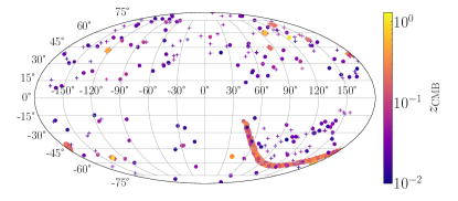
Figure 1: Sky coverage of the supernova samples used in this work. Crosses show the sky location of Pantheon supernovae and circles show the JLA supernovae in galactic coordinates $(l,b)$. Each point is coloured according to the redshift of that supernova in the CMB frame, $z_{\rm CMB}$.

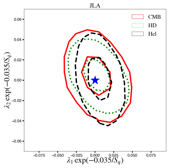
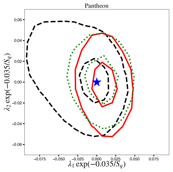
Figure 2: Constraints on the eigenvalues of the quadrupole of the Hubble parameter using the JLA (left) and Pantheon (right) datasets. The contours are obtained with the $\chi^{2}$ method with redshifts in the CMB frame (solid red), heliocentric frame (dashed black) and HD redshifts (dotted green). The contours show the 1- and 2-$\sigma$ limits. We find no significant evidence for deviation from isotropy (marked with the blue star) in any of the cases studied here.

3.3 Datasets

We use the most recent SN Ia lightcurve parameters and redshift data from the JLA (Betoule et al., 2014) and Pantheon (Scolnic et al., 2018) compilations. Figure 1 shows the sky coverage of the two samples, with crosses showing Pantheon supernovae directions and circles showing JLA supernovae directions. All points are coloured according to the redshift of the supernova in the CMB frame, $z_{\rm CMB}$ (as defined below).

The cosmographic representation of the luminosity distance (1) is generically expected to be divergent for $z>1$ (Cattoen & Visser, 2007; Macpherson & Heinesen, 2021). However, the approximation of the Taylor series to the exact distance formula in isotropic cosmology is expected to be reasonable for redshifts close to 1 (e.g., see Arendse et al., 2020), at least for testing cosmologies close to the $\Lambda$CDM model (Aviles et al., 2014). Most Over 97% of SNe Ia in the JLA and Pantheon datasets have $z<1$, with the SN Ia with the largest redshift has highest-redshift SN Ia being $z=1.3$ and $z=2.3$, respectively. Hence, for the majority of SNe Ia, the Taylor series should provide a valid description of the distances. We therefore adopt the cosmographic representation for all SNe Ia in both samples. The anisotropic features that we are constraining are exponentially decaying with redshift and thus the main results of our analysis are predominantly determined by the lowest-redshift SNe Ia in the sample.

Peculiar velocity (PV) corrections based on estimates within the $\Lambda$CDM model are usually applied to the measured redshifts of nearby SNe Ia in order to alleviate the motions of these SNe Ia with respect to the CMB frame. There has been a recent debate in the literature about the consistency of these corrections and their impact on the evidence for cosmic acceleration (Colin et al., 2019a; Rubin & Heitlauf, 2020). Therefore, we evaluate the impact of PV corrections on our constraints by presenting results inferred from three different redshift frames. We consider: 1) Heliocentric (Hel) redshifts: the measured redshifts of each SN Ia in the heliocentric frame; 2) CMB-frame redshifts: the heliocentric redshifts corrected via a boost of the Earth to the CMB frame (using the CMB dipole as inferred by Planck Collaboration, 2020a); and 3) Hubble diagram (HD) redshifts: CMB-frame redshifts with PV corrections applied to individual SNe Ia. We will adopt the CMB-frame redshifts in our fiducial analysis. While redshifts in the heliocentric frame are not usually used for parametrising distances at cosmological scales, they are useful as a reference in model-independent analysis, e.g. in cases where we might not wish to assume that the dipole in the CMB is a purely observer-kinematic effect. As part of our analysis, we will also fit for the best-fit rest frame — i.e., not a priori constraining this to be the CMB frame — for both samples of SNe Ia.

Previous studies using various SN Ia compilations and data reduction methods have reached differing conclusions about the significance of a dipole in the deceleration parameter. Some works have found no significant dipole and report consistency with the $\Lambda$CDM model (Soltis et al., 2019; Zhao et al., 2019; Rubin & Heitlauf, 2020), while others claim a deviation from isotropy at a level that challenges the use of the FLRW geometry at low redshift (Cai & Tuo, 2012; Bengaly, 2016; Colin et al., 2019b). Motivated by this discrepancy, we study of the impact of different analysis assumptions on the constraints of the dipole in the deceleration parameter. In particular, we test the impact of the PV corrections (through the use of the three different redshift frames outlined above) on both datasets.

Table 1: Parameter priors used in the inference for each of the models tested in this work in both the JLA and Pantheon analyses.

Parameter	Prior	Multipole model implemented in
$q_{m}$	U[-4, 4]	Quadrupole and Dipole
$j_{0}-\Omega_{k}$	U[-10, 10]	Quadrupole and Dipole
$q_{d}$	U[-10, 10]	Dipole
$S_{d}$	U[0.01, 4]	Dipole
$\lambda_{1}$	U[-2, 2]	Quadrupole
$\lambda_{2}$	U[-2, 2]	Quadrupole
$S_{q}$	U[0.01, 4]	Quadrupole

For the JLA dataset, we also analyse the role of the PV covariance matrix and distance bias corrections. The latter are applied to $m_{B}$ after the corrections to light-curve width, colour, and host galaxy mass, in order to account for systematics arising from survey selection criteria (see Betoule et al., 2014; Scolnic et al., 2018, for more details on these corrections). For the Pantheon dataset, corrections for the width- and colour-luminosity relation and distance biases to the SN Ia distances have been applied before the data was made public. Therefore, we only test the impact of PV corrections on results using the Pantheon sample. In Appendix A, we fit the nuisance parameters simultaneously with the cosmology and show that we obtain similar constraints as in our main analysis of the Pantheon sample.

4 Results

Table 2: Summary of constraints on the isotropic deceleration and curvature minus jerk parameters $q_{m}$ and $j_{0}-\Omega_{k}$, the eigenvalues of the quadrupole in the Hubble parameter $\lambda_{1}$ and $\lambda_{2}$, and the exponential decay scale of the quadrupole, $S_{q}$. All results shown here are found using the $\chi^{2}$ method.

Dataset	Redshift	$q_{m}$	$j_{0}$ - $\Omega_{\rm K}$	$\lambda_{1}$	$\lambda_{2}$	$S_{q}$
JLA	CMB	-0.316 ${}^{+0.115}_{-0.117}$	-0.373 ${}^{+0.403}_{-0.49}$	0.005 ${}^{+0.017}_{-0.023}$	0.002 ${}^{+0.022}_{-0.017}$	0.974 ${}^{+0.98}_{-0.974}$
JLA	HD	-0.392 ${}^{+0.122}_{-0.11}$	-0.109 ${}^{+0.521}_{-0.494}$	0.003 ${}^{+0.012}_{-0.015}$	0.005 ${}^{+0.015}_{-0.012}$	1.258 ${}^{+0.901}_{-1.258}$
JLA	Hel	-0.404 ${}^{+0.116}_{-0.113}$	-0.115 ${}^{+0.47}_{-0.562}$	0.006 ${}^{+0.013}_{-0.016}$	0.001 ${}^{+0.013}_{-0.014}$	1.253 ${}^{+0.962}_{-1.252}$
Pantheon	CMB	-0.448 ${}^{+0.076}_{-0.081}$	0.264 ${}^{+0.289}_{-0.374}$	0.011 ${}^{+0.008}_{-0.01}$	-0.003 ${}^{+0.01}_{-0.009}$	1.564 ${}^{+0.853}_{-1.554}$
Pantheon	HD	-0.481 ${}^{+0.078}_{-0.067}$	0.38 ${}^{+0.331}_{-0.335}$	0.072 ${}^{+1.552}_{-0.907}$	-0.136 ${}^{+0.663}_{-1.816}$	0.002 ${}^{+0.001}_{-0.002}$
Pantheon	Hel	-0.49 ${}^{+0.078}_{-0.073}$	0.408 ${}^{+0.283}_{-0.399}$	-0.007 ${}^{+0.022}_{-0.019}$	0.003 ${}^{+0.015}_{-0.017}$	0.275 ${}^{+1.096}_{-0.265}$

We present our inferred constraints on the quadrupole of the Hubble parameter in Section 4.1, and on the dipole of the deceleration parameter in Section 4.2. We constrain these independently, i.e., when constraining the quadrupole, we set the dipole term to zero, and vice versa. We perform Bayesian analysis based on the constrained $\chi^{2}$ metod for both the JLA and the Pantheon sample of SNe Ia, and consider an independent frequentist MLE analysis for the JLA sample. The priors that we use for each model parameter in the Bayesian analyses are summarised in Table 1.

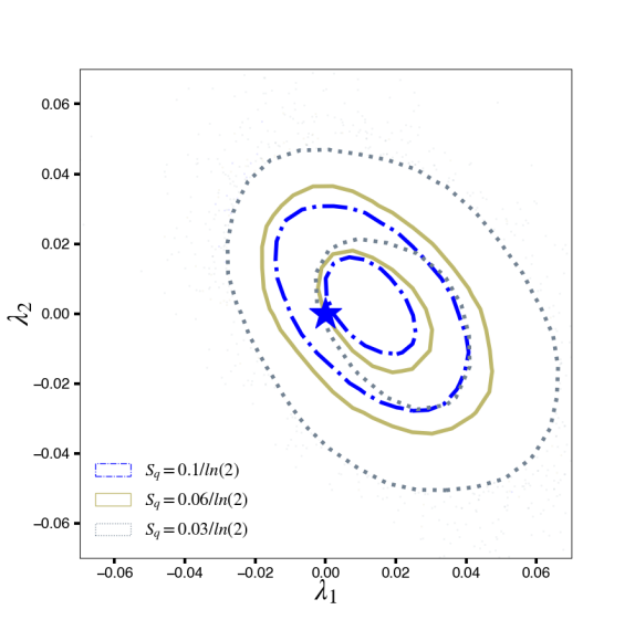
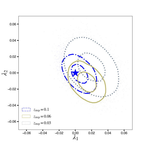
Figure 3: Constraints on the eigenvalues of the quadrupole $\lambda_{1}$, $\lambda_{2}$ for the parametrisations with a fixed scale (left) and fixed redshift step value (right). The scale values are varied between $\frac{0.03}{ln(2)},\frac{0.06}{ln(2)}$, and $\frac{0.1}{ln(2)}$ and the redshift steps at $0.03,0.06$, and 0.1. As expected, the constraints are worsened for small step values since there are fewer SNe Ia in the redshift range. All cases are consistent with isotropy.

4.1 Constraints on the quadrupole

For the constraints on the quadrupole we use the exponential decay model for $\mathcal{F}(z,S_{q})$ as the fiducial case with the scale as a free parameter. We also evaluate the constraints with the scale parameter fixed as well as a step function in redshift, as described in Section 2.3.

Parnovsky & Parnowski (2013) constrained the dipole, quadrupole, and octupole moments of the bulk motion of a set of nearby galaxies. We fix the eigendirections of the quadrupole in the Hubble parameter to coincide with their best-fit results of $\boldsymbol{\theta}_{1}$=(118,85)°, $\boldsymbol{\theta}_{2}$=(341,4)°, and $\boldsymbol{\theta}_{3}$=(71,-4)° in galactic angular coordinates $(l,b)$. With these eigendirections, we then constrain the eigenvalues of the quadrupole, $\lambda_{1}$ and $\lambda_{2}$, and its decay scale $S_{q}$, along with the monpolar parameters $q_{m}$ and $j_{0}-\Omega_{K}$ of the analysis. We have repeated the analysis allowing the eigendirections $\boldsymbol{\theta}_{1},\boldsymbol{\theta}_{2},$ and $\boldsymbol{\theta}_{3}$ to vary, and have found no significant improvements in the profile likelihood for any alternative eigenbasis.

Figure 2 shows our constraints on the quadrupole in the Hubble parameter as obtained from the JLA and the Pantheon datasets using the $\chi^{2}$ method. We show the amplitude of the quadrupole contribution at redshift $z=0.035$ (or on scales of $\sim 100h^{-1}$ Mpc), namely$\lambda_{1}\,{\rm exp}(-0.035/S_{q})$ and $\lambda_{2}\,{\rm exp}(-0.035/S_{q})$. Dashed black contours show constraints using the heliocentric redshifts, solid red contours show those using CMB-frame redshifts, and dotted green contours show those using HD redshifts. Our results are consistent with zero in all cases and show no significant change between redshift frames.

In Table 2 we summarise our constraints on all parameters for both the JLA and Pantheon datasets obtained with the $\chi^{2}$ method. We show constraints using heliocentric, CMB-frame, and HD redshifts for both datasets. For all cases, we find results consistent with $\lambda_{1}=\lambda_{2}=0$ at the $\sim 1\sigma$ level. From the 95$\%$ confidence level in Figure 2 and using (15), we place an upper limit on the total quadrupole amplitude of $\sim 10\%$ at scales of $\sim 100\,h^{-1}$ Mpc (or $z=0.035$). Therefore, the few-percent quadrupole predicted in (Macpherson & Heinesen, 2021) is consistent with current data. In Section 4.3, we forecast improvements on our constraint for upcoming low-redshift surveys such as the Zwicky Transient Facility (ZTF; Dhawan et al., 2022) or the Young Supernova Experiment (YSE; Jones et al., 2021).

Table 3: Constraints on the isotropic deceleration and curvature minus jerk parameters $q_{m}$ and $j_{0}-\Omega_{k}$, the eigenvalues and exponential decay of the quadrupole in the effective Hubble parameter, $\lambda_{1},\lambda_{2}$, and $S_{q}$. Results here are found using the MLE method and the JLA SN Ia dataset. The $m_{B}$ bias corrections are removed and $\sigma_{z}$ is set to zero. The p-value in the right-most column is the probability of the null hypothesis (isotropic universe model) relative to the model with a non-zero quadrupole.

Redshift	$q_{m}$	$j_{0}-\Omega_{\rm K}$	$\lambda_{1}$	$\lambda_{2}$	$S_{q}$	p-value
CMB	-0.160	-0.455	0.109	-0.0396	0.0110	0.67
HD	-0.260	-0.159	4.78	-4.27	0.0028	0.67
Hel	-0.151	-0.496	-0.00713	0.0095	24.8	0.81

Table 3 shows our constraints on the quadrupole parameters using the MLE method for all three redshift frames. For all cases, our results are consistent with isotropy (zero quadrupole) at the $\sim 1\sigma$ level, which can be seen from the p-value for the isotropic null hypothesis as quoted in the right-most column of the table.

We also test two different parametrisations of the quadrupole that determine the redshift region where the quadrupole dominates. First, we fix the exponential decay scale to $S_{q}=0.03/{\rm ln}(2),0.06/{\rm ln}(2)$, and $0.1/{\rm ln}(2)$. These choices imply ${\rm exp}(-z/S_{q})=1/2$ for redshifts $z=0.03,0.06$, and 0.1, respectively. Second, we treat the quadrupole as a step function in redshift, i.e. we set $\mathcal{F}(z\leq z_{\rm step}{,z_{\rm step}})=0$ and $\mathcal{F}(z>z_{\rm step}{,z_{\rm step}})=1$ for $z_{\rm step}=0.03,0.06$, and 0.1. These redshift values all lie in the low-$z$ (i.e. $z\leq 0.1$) regime — where we expect the anisotropy to be strongest — while still being sufficiently above the minimum redshift in the SN Ia compilations. The left panel of Figure 3 shows the posterior distribution for the eigenvalues of the quadrupole, using the $\chi^{2}$ method, for the three exponential decay profiles for the Pantheon sample. The right panel of Figure 3 shows the same constraints for the three cases of the step function. We find similar constraints for the both the fixed redshift step and the exponential decay model with the fixed decay scale. For all cases shown here we use the CMB frame redshifts, however, we find similar results for the Helicontric and HD frame redshifts, all indicating a quadrupole feature consistent with zero at the $\sim 1\sigma$ level. In all of these cases, we thus find no significant deviation from the isotropic null hypothesis. We also find that performing the same fits with the JLA sample gives consistent results.

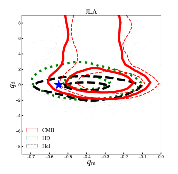
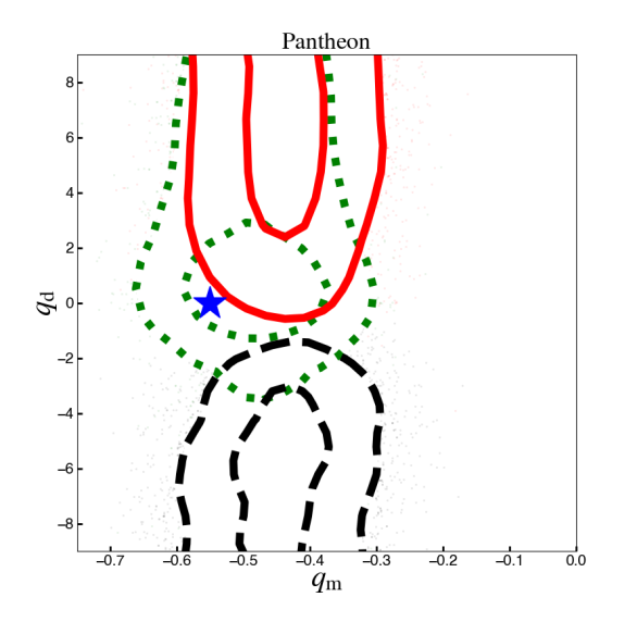
Figure 4: Left panel: Constraints on the monopole and dipole terms of the deceleration parameter using the JLA compilation. The constraints are shown for the heliocentric (thick dashed black), CMB frame redshift (solid red) and the HD redshifts (dotted green). All contours contain the PV covariance matrix. Thin dashed red contours in the left panel show the CMB frame constraints without the distance bias corrections. Right panel: The same constraints for the Pantheon compilation. All contours represent the 1- and 2-$\sigma$ constraints.

4.2 Dipole of the deceleration parameter

In our main analysis, we set the direction of the dipole in the effective deceleration parameter to coincide with the CMB dipole as found by Planck Collaboration (2020a), namely $(l,b)$ = (264.021, 48.523)°. In order to ensure that the CMB dipole direction is indeed an optimal direction for the dipolar signature, we test for the best-fit direction by varying the dipole direction and comparing the likelihood of the fit for different directions on the sky (see Appendix B). Using the MLE method, we find the direction that optimises the profile Likelihood function to closely coincide with the direction of the CMB dipole, as was also found in Colin et al. (2019b).

The left panel of Figure 4 shows our constraint contours in the $q_{d}$–$q_{m}$ plane for the JLA dataset using the $\chi^{2}$ method, including the PV covariance matrix. The right panel shows the same constraints for the Pantheon dataset. In both panels, solid red contours show the results from CMB-frame redshifts, dotted green contours show HD redshifts, and thick dashed black contours show heliocentric redshifts. All constraints include the distance bias corrections, with the exception of the thin dashed red contours in the left panel, which show the CMB-frame constraints for JLA with these corrections removed. Removing these corrections does not significantly impact our constraints, and so we retain them for the rest of our analysis.

We summarise our constraints on the deceleration parameter using the $\chi^{2}$ method in both the JLA and Pantheon data in Table 4. We show constraints on the monopole $q_{m}$, the dipole amplitude $q_{d}$, the decay scale $S_{d}$, and the (isotropic) jerk minus curvature parameter $j_{0}-\Omega_{K}$. We show all three redshift cases with PV covariance included in the estimated errors, as well as the CMB and heliocentric redshifts without PV covariance contributions (see Betoule et al., 2014, for details on the components of the covariance matrix). For the JLA dataset, we find $q_{d}=2.18^{+3.353}_{-2.724}$ for the CMB frame redshifts, and when adding the PV corrections we find $q_{d}=-0.004^{+1.08}_{-0.785}$. In all but one case, the JLA dataset yields a dipole consistent with zero. In the case of JLA heliocentric redshifts without the PV covariance matrix, we find a significant dipole at the $3.3\sigma$ level. For the rest of this work, we compute the significance of our results as $\sqrt{2}$ times in the inverse error function of the $n^{\rm th}$ percentile that is consistent with isotropy, i.e. $q_{d}=0$. For Pantheon, both heliocentric and CMB-frame redshifts yield a dipole at $3.43\sigma$ and $2.17\sigma$ significance, respectively (including the PV covariance matrix). After applying the PV corrections (i.e. using HD redshifts), the dipole is consistent with zero within $1\sigma$ for both samples.

Comparing the constraints from the JLA and Pantheon compilations in the left and right panels of Figure 4, respectively, we find that the posterior distributions are similar for the CMB and HD redshifts, with the $1\sigma$ contours of the two samples (close to) overlapping. For redshifts in the heliocentric frame, we find an overlap of the 2 $\sigma$ contours (but not the $1\sigma$ contours), which indicates a moderate inconsistency between the two samples. We note that there have been several updates between the two compilations, e.g. the redshift measurements for a subsample, additional objects at high-$z$ photometric calibration, retraining of the lightcurve fitting method. We remade the constraints in Figure 4 using only the SNe Ia in common between the two compilations as well as using the same redshift measurement reported for $z_{\rm hel}$ — i.e., by using $z_{\rm hel}$ reported in one sample for all objects with the respective magnitudes from each sample, and vice versa. However, in both of these tests we still find an inconsistency between the samples at the $\lesssim 2\sigma$ level. We therefore cannot attribute this inconsistency to the difference in objects between the samples or in any difference in reported redshifts. The source of the systematic differences pointed out here are important to clarify and should be further investigated with larger, improved samples such as the Pantheon+ compilation (Brout et al., 2022).

Table 4: The median and 68$\%$ C.L. constraints on the monopole and dipole moments of the deceleration parameter for both JLA and Pantheon compilations. Here we compute the parameters for the CMB frame, HD (see text for details) and heliocentric frame redshifts. We also evaluate the parameters with and without the covariance matrix for the peculiar velocity corrections (for the CMB and heliocentric frames) for the JLA compilation.

Dataset	Covariance	Redshift	$q_{m}$	$j_{0}$ - $\Omega_{\rm K}$	$q_{d}$	$S_{d}$
JLA	With PV cov	CMB	-0.348 ${}^{+0.128}_{-0.107}$	-0.28 ${}^{+0.404}_{-0.558}$	1.016 ${}^{+3.262}_{-1.561}$	0.143 ${}^{+0.006}_{-0.006}$
JLA	With PV cov	HD	-0.413 ${}^{+0.124}_{-0.119}$	-0.048 ${}^{+0.446}_{-0.623}$	0.034 ${}^{+0.737}_{-0.322}$	0.141 ${}^{+0.007}_{-0.006}$
JLA	With PV cov	Hel	-0.399 ${}^{+0.115}_{-0.113}$	-0.129 ${}^{+0.511}_{-0.501}$	-0.066 ${}^{+0.167}_{-0.447}$	0.142 ${}^{+0.006}_{-0.006}$
JLA	Without PV cov	CMB	-0.343 ${}^{+0.103}_{-0.122}$	-0.296 ${}^{+0.405}_{-0.553}$	2.379 ${}^{+2.868}_{-2.609}$	0.026 ${}^{+0.035}_{-0.026}$
JLA	Without PV cov	Hel	-0.315 ${}^{+0.121}_{-0.104}$	-0.380 ${}^{+0.449}_{-0.465}$	-6.806 ${}^{+1.087}_{-3.189}$	0.028 ${}^{+0.008}_{-0.009}$
Pantheon	With PV cov	CMB	-0.439 ${}^{+0.076}_{-0.073}$	0.240 ${}^{+0.325}_{-0.323}$	5.414 ${}^{+4.486}_{-1.705}$	0.020 ${}^{+0.007}_{-0.009}$
Pantheon	With PV cov	HD	-0.481 ${}^{+0.073}_{-0.071}$	0.373 ${}^{+0.295}_{-0.374}$	0.696 ${}^{+4.002}_{-1.19}$	0.021 ${}^{+0.034}_{-0.021}$
Pantheon	With PV cov	Hel	-0.445 ${}^{+0.076}_{-0.078}$	0.252 ${}^{+0.303}_{-0.365}$	-6.001 ${}^{+2.037}_{-3.111}$	0.027 ${}^{+0.007}_{-0.01}$

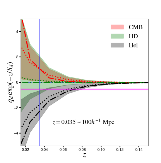
Figure 5: The evolution of the deceleration parameter dipole with redshift. We show the dipole amplitude as a function of redshift in the CMB (red), HD (green) and heliocentric (black) frames. The solid lines are the inferred values from the $\chi^{2}$ method applied to the JLA data (without PV covariance matrix for a direct comparison with the MLE method), whereas the dotted lines are for the $\chi^{2}$ method applied to the Pantheon data. The dashdot lines are the result from the MLE method applied to the JLA data. Shaded regions show the 2-$\sigma$ bounds for the $\chi^{2}$ constraints. The shaded region are the 2-$\sigma$ bounds for the constraints from the $\chi^{2}$ method for the Pantheon compilation. The magenta line shows the magnitude of the monopole in the standard cosmological model, for comparison.

For the Pantheon dataset, the reported magnitudes have already been calibrated for stretch, colour, and host galaxy properties of the SNe Ia , within a cosmological model. We can therefore only use the constrained $\chi^{2}$ model for the Pantheon dataset. In Appendix A, we test the impact of these magnitude calibrations on the cosmological constraints, by repeating the analysis using the light curve parameters provided with the Pantheon compilation. We find no correlation between the SN Ia standardisation and the cosmological parameters of our analysis. Our results with the corrected $m_{B}$ Pantheon data in the main analysis are thus recovered within the more model-independent approach examined in Appendix A.

Table 5: Constraints on the isotropic deceleration and curvature minus jerk parameters $q_{m}$ and $j_{0}-\Omega_{k}$, and the magnitude and exponential decay scale of the dipole in the effective deceleration parameter, $q_{d}$ and $S_{d}$. Results here are obtained with the MLE method and the JLA SN Ia data set. The $m_{B}$ bias corrections are removed and $\sigma_{z}$ is set to zero. The p-value in the right-most column is the probability of the null hypothesis (isotropic universe model) relative to the model with a non-zero dipole.

Redshift	$q_{m}$	$j_{0}$ - $\Omega_{\rm K}$	$q_{d}$	$S_{d}$	p-value
CMB	-0.174	-0.416	14.1	0.0122	0.024
HD	-0.256	-0.174	10.4	0.00084	0.67
Hel	-0.158	-0.488	-8.13	0.0261	$7.9\times 10^{-5}$

Table 5 shows our constraints on the deceleration parameter for the JLA dataset using the MLE method. Again, we consider all three redshift cases. For the HD redshifts, the dipole signal is consistent with zero. For the heliocentric redshifts, we find a significant dipole with best fit values $q_{d}=-8.13$ and $S_{d}=0.0261$ and p-value $=7.9\times 10^{-5}$. This result is consistent with the equivalent case in Table 4 (heliocentric redshifts without PV cov) using the $\chi^{2}$ method. In the CMB frame, we find a preferred dipole with opposite sign of that in the heliocentric frame, albeit the significance of the signature is lowered. The change of sign of the preferred dipole in the deceleration parameter is due to the partial degeneracy between this dipole and the special-relativistic boost of the observer (see Section 5 of Heinesen, 2020). This result differs from that of the analogous analysis using the $\chi^{2}$ method, for which we found no significant dipole signature.

So far in our analysis, we have maintained the velocity of the observer to coincide with the best-fit velocity as inferred from the dipole in the CMB. If the dipole anisotropy in SN Ia data is purely due to our kinematic motion and the CMB dipole is of purely kinematic origin as well, we should infer a similar observer velocity to that obtained from the CMB. We now leave the amplitude of the observer velocity as a free parameter in an isotropic analysis, maintaining the direction fixed to that of the CMB dipole. We have repeated the analysis, allowingthe direction to vary, and find the maximum likelihood direction to closely coincide with that of the CMB dipole (see Appendix B). For this test, we neglect the PV covariance contributions to the total error covariance matrix. Inclusion of PV covariance increases the error bars by $\sim 20\%$, but gives overall similar results to those quoted below. For the JLA SNe Ia, we find a velocity $v=258.15^{+57.9}_{-61.2}$ km/s relative to the heliocentric frame using the constrained $\chi^{2}$ method and $v=252$ km/s using the MLE method (with a p-value of $0.018$). Both of these velocities are consistent with the recent result in Horstmann et al. (2021), however, both are discrepant from that inferred from the CMB dipole ($369.82\pm 0.11$ km/s; Planck Collaboration, 2020a). Using the $\chi^{2}$ method for the Pantheon SNe Ia, we find a best-fit velocity of 240 ${}^{+57.0}_{-36.2}$ km/s, which is in agreement with our other results. This suggests an additional contribution to the dipole in SNe Ia data beyond that of a special-relativistic boost of the observer to the rest-frame of the CMB.

We found a significant dipole in the deceleration parameter using the MLE method for the case of JLA SNe Ia in the heliocentric frame (see Table 5), with an observer velocity coinciding with that inferred from the CMB dipole. Instead keeping the observer velocity as a free parameter in this anisotropic analysis — i.e., allowing both the kinematic and geometric dipoles to be free parameters — removes the significance of $q_{d}\neq 0$. Thus, we find that the dipole in the deceleration parameter is consistent with zero only if the frame of reference is different to the rest-frame of the CMB. However, the HD frame results in Table 5 also show an insignificant dipole in the deceleration parameter. Thus, we conclude that the SN Ia PV estimates in standard analyses can account for the dipole in the deceleration parameter that we find here. Peculiar flows are indeed expected to give rise to anisotropies in the Hubble law of the type investigated in this paper, as we comment on in the discussion.

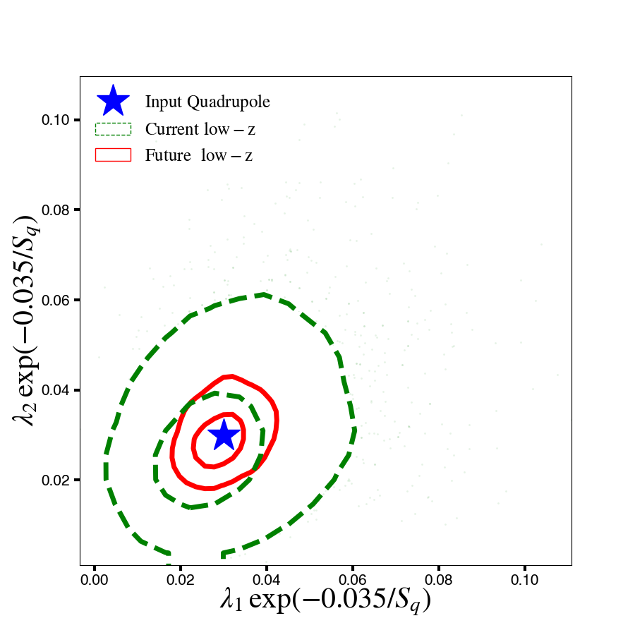
Figure 6: Posterior distribution of $\lambda_{1}\cdot{\rm exp}(-z/S_{q})$, $\lambda_{2}\cdot{\rm exp}(-z/S_{q})$ for the artifical input model with a 2.9% quadrupole at $z=0.035$, corresponding to $\sim$100 $h^{-1}$ Mpc scales. The forecasts for a SN Ia compilation of the same size as the current Pantheon compilation is shown as green contours, and for a compilation with 5 $\times$ larger low-$z$ anchor samples is shown as red contours. Contours show the 1- and 2-$\sigma$ regions, respectively. We mark the input quadrupole value in our forecasts with a blue star.

In Figure 5 we show the exponentially-decaying dipole amplitude as a function of redshift for the different statistical methods and datasets used here. Different colours represent the three redshift frames we use, as indicated in the legend. Solid lines show best-fit values obtained using the $\chi^{2}$ method with JLA SNe Ia, dotted lines show $\chi^{2}$ best-fit values for Pantheon SNe Ia, and dot-dashed lines show results using the MLE method with JLA SNe Ia. Shaded regions show the 2-$\sigma$ bounds for the $\chi^{2}$ constraints. The horizontal magenta line shows the magnitude of the monopole, for comparison, and the vertical blue line marks the scale $z=0.035$ corresponding to a distance scale of $\sim 100h^{-1}$ Mpc. The Pantheon data using the CMB frame redshifts marginally suggests a non-zero dipole at the $\sim 2\sigma$ level, whereas we find no suggestion of a dipole when using the HD redshifts. We find a significant dipole in both datasets when using the heliocentric redshifts. This figure is a summary of our main results, while illustrating the redshift ranges for which a non-zero dipole (with this parametrisation) might be important.

Crucially, we find that in both left and right panels of Figure 4, the posterior distribution of the monopole $q_{m}$ is not significantly correlated with the value of the dipole $q_{d}$. Hence, the assumption on the value of $q_{d}=0$ in the isotropic cosmography does not significantly impact the inferred $q_{m}$. Further, from both Figure 4 and Table 4, we can see that the boost to the CMB frame, and the PV corrections, do not significantly impact the inferred value of the monopole, $q_{m}$, when using the $\chi^{2}$ method. Inferences of $q_{0}$ using isotropic cosmography in the literature (e.g. Bernal et al., 2016; Lemos et al., 2019; Feeney et al., 2019) are consistent with the $q_{m}$ value we find with the $\chi^{2}$ method at the 1–2$\sigma$ level. Our results using the MLE method also show minimal change in the value of the monopole $q_{m}$ with redshift frame (see Table 5). However, the values of the monopole in the heliocentric and CMB frames are $q_{m}=-0.158$ and $q_{m}=-0.174$, respectively, which deviate from the value within $\Lambda$CDM of $q_{0}\approx-0.55$. The likely cause of this difference between the two methods is the assumption of the redshift evolution of the population of SNe Ia lightcurve width ($x_{1}$) and colour ($c$) parameters. The $\chi^{2}$ method accounts for survey selection as a function of redshift whereas the MLE method assumes no redshift dependence in the distributions of the intrinsic supernova parameters. Since the SN Ia surveys are impacted by Malmquist bias, i.e., they preferentially detect brighter SNe Ia at higher redshifts, the failure to account for such bias, or doing so in an incorrect manner, can impact the value of the monopole term $q_{m}$. Such an impact has been recently discussed in the literature Colin et al. (2019a); Rubin & Heitlauf (2020). Our findings agree with both Colin et al. (2019a) and Rubin & Heitlauf (2020) for the relevant statistical method, and therefore further investigation into the appropriate way of accounting for survey selection as a function of redshift is necessary to clarify this debate.

4.3 Forecast of constraints on the quadrupole in the Hubble parameter

Ongoing and future surveys will discover a large number of SNe Ia. ZTF and YSE will increase the low-redshift SN Ia sample and significantly improve systematic errors. For regional anisotropies that decay towards larger scales, improvements in low-redshift data will make the most difference to our constraining power. In this section, we forecast the constraints on the quadrupole in the Hubble parameter from the improved low-$z$ samples. We start with a simulated realisation with uncertainties corresponding to the current Pantheon compilation, and then increase the number of low-$z$ samples to coincide with expected future datasets.

We infer distances to SNe Ia for an input model with a quadrupole in the Hubble parameter such that $\lambda_{1}\cdot{\rm exp}(-z/S_{q})=\lambda_{2}\cdot{\rm exp}(-z/S_{q})=0.029$ in (12) at $z=0.035$. This induced $\sim 7\%$ quadrupole amplitude is motivated both by the upper limit on the quadrupole we find here as well as the numerical results obtained by Macpherson & Heinesen (2021). In the latter, the authors found a quadrupole in the Hubble parameter of a few percent on $\sim 100h^{-1}$ Mpc scales in a set of general-relativistic cosmological simulations. We take the redshift and distance modulus error distribution of the mock SNe Ia to be the same as the Pantheon data. We augment the low-$z$ ($z\leq 0.1$) anchor sample to five times its size such that the total number of low-$z$ SNe Ia is 1055. This sample size is conservatively well within the limit of data already obtained by current and ongoing low-$z$ SN Ia surveys. For comparison, we also use simulated distances for a low-$z$ anchor sample of the same size as the current Pantheon compilation.

Figure 6 shows our forecast constraints for the input cosmology with a non-zero quadrupole for a future low-$z$ survey (solid red contours) and for a sample consistent with current low-$z$ catalogues (dashed green contours). The blue star represents the values of the input cosmology. We find that the improved low-$z$ anchor sample will be able to detect a 7% quadrupole at 100 $h^{-1}$ Mpc scales with 5$\sigma$ significance.

5 Discussion and Conclusion

The assumption of isotropy is a central feature of the standard cosmological model and must be empirically tested. Any universe with structure will necessarily contain anisotropies in the $d_{L}$–$z$ relation. Therefore — once the data is precise enough to resolve such anisotropies —, anisotropic contributions to low-redshift data need to be included for a realistic cosmological fit. Such anisotropies could also impact local distance determinations, e.g., those based on Cepheids (Riess et al., 2021) or TRGB (Freedman, 2021), in the case of an anisotropic distribution of SNe Ia. In this work, we have presented the first constraints on the theoretically motivated quadrupole moment of the effective Hubble parameter in the distance-redshift relation. The quadrupole moment physically arises from the anisotropic expansion of space around the observer as incorporated in the shear tensor. Using the SN Ia magnitude-redshift relation, we find no significant quadrupole in the effective Hubble parameter, with our best-fit quadrupole amplitude being consistent with zero. This constraint holds for both the JLA and Pantheon compilations, and is robust to the changes in redshift frames and likelihood methods considered here. Our results are unchanged when including $\Lambda$CDM modelled corrections for peculiar motions of the SNe Ia with respect to the CMB frame.

We have placed an upper bound of $\sim 10\%$ for the quadrupolar anisotropy within our exponential decay model (using Eq. 15). Since the decay scale can be degenerate with the value of the eigenvectors, we also constrain the parametrisations with a fixed decay scale, as well as a fixed step value in redshift, and find results consistent with the fiducial model. We stress again that this anisotropic contribution to the Hubble parameter is not degenerate with the SN Ia absolute luminosity, unlike the monopole $H_{m}$. It can therefore be constrained by the magnitude-redshift relation of SNe Ia without needing external calibrators to first constrain the SN Ia absolute magnitude prior to the cosmological fit.

Parnovsky & Parnowski (2013) used the Revised Flat Galaxy Catalogue (RFGC) to constrain the quadrupole (shear) at the 100 $h^{-1}$ Mpc scale, finding eigenvalues of ${\lambda}_{1}=7.27{\%}\pm 1.54{\%}$ and ${\lambda}_{2}=-2.43{\%}\pm 1.46{\%}$. Since we use the same eigendirections as the RFGC study, we can compare our constraints to their results. The RFGC quadrupole was found to be almost constant over the 80–170 $h^{-1}$ Mpc scales which they considered, therefore, our quadrupole constraints from the step function parametrisation (with $z_{\rm step}=0.03$) are the closest in formalism to the RFGC study. We find agreement between our results and the RFGC measurements at the $\sim$2$\sigma$ level (but not at the 1$\sigma$ level). It is important to constrain this quadrupolar anisotropy with future larger datasets, as well as with independent probes.

We have also forecasted the precision of quadrupole measurements from future low-$z$ SN Ia surveys. This forecast is timely, since the number of SNe Ia available for cosmological studies will increase manyfold within this decade. With upcoming samples of SNe Ia in the nearby Hubble flow, e.g., from ZTF or YSE, we can significantly improve the constraints on the quadrupole moment of the Hubble parameter. For our input signal we took a quadrupole with $\sim 7\%$ amplitude to test whether it can feasibly be constrained with future surveys. Specifically, we forecast that with $1055$ SNe Ia we will have the potential to detect this quadrupole at $5\sigma$ significance. A sample of this size is also interesting for constraining the kinematic nature of the CMB dipole (e.g. Horstmann et al., 2021). Hence, the improved low-$z$ data will be important for tests of the cosmic rest frame.

We have also presented constraints on the dipole in the deceleration parameter. We focused on the impact of the statistical method as well as input data assumptions. We find that for the JLA compilation, the dipole is consistent with zero at the $1\sigma$ level when inferred using the $\chi^{2}$ method for all but one case. The only instance of a significant dipole occurs in the heliocentric frame without applying the PV covariance matrix. With the same inference method, we find that the Pantheon compilation indicates marginal significance of a dipole at the $\sim 2\sigma$ level when using the CMB frame, however, this dipolar signature vanishes when applying the PV corrections to the SN Ia redshifts. We note that for the MLE method, we similarly find that the CMB frame redshifts with PV corrections are consistent with isotropy. However when PV corrections are not applied, we find a significant dipole in both the CMB and heliocentric frame. In Figure 5, we have presented a summary of the dipole amplitude for the exponentially decaying case, illustrating its dependence on redshift for both statistical methods and datasets used here, as well as all redshift frames.

Recent improvements in the treatment of PV corrections have been shown to have a small impact on parameter constraints in isotropic cosmologies (e.g. for $H_{0}$ in Peterson et al., 2021). In addition, Rahman et al. (2021) used an improved flow model to correct for PVs and found no evidence for departures from isotropy once the PV corrections were applied, consistent with our findings. The theoretical framework developed by Heinesen (2020) in principle allows us to account for anisotropic expansion of space and to infer peculiar velocities around a background model for both the observer and the sources. This will be a possibility with future low-$z$ SN Ia samples that have significantly increased statistics. It will be interesting to further tighten the constraints on anisotropies we find here using upcoming improved SN Ia magnitude-redshift data (e.g. Brout et al., 2022).

Data Availability

The data for the analysis is public and the software used is entirely based on publicly available packages and will be made available upon request.

Appendix A Dependence on nuisance parameters

The JLA supernova compilation provides a catalog of peak apparent magnitude, $m_{B}$, light curve width, $x_{1}$, and colour, $c$, values along with the host galaxy masses. We therefore can marginalise over the nuisance parameters in the luminosity standardisation relation in (17). For the Pantheon compilation, however, the publicly-available apparent luminosity has already been corrected for the width-luminosity and color-luminosity relations. However, this fit was explicitly based on the FLRW metric. We, therefore, verify the impact of these corrections by marginalising the SN Ia width-luminosity, colour-luminosity and host galaxy mass distributions along with the cosmological parameters for our model. For this we use the publicly available lightcurve fit parameters and host galaxy masses for the Pantheon SNe Ia.

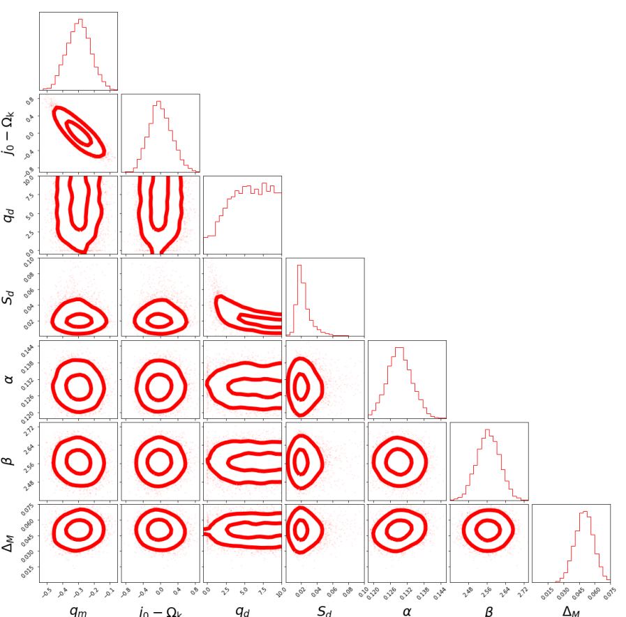
Figure 7: Posterior distribution of the cosmological and SN Ia nuisance parameters using the Pantheon compilation. We find that cosmological parameters for the model are not correlated with the nuisance parameters for SN Ia standardisation relations. The contours are 1- and 2-$\sigma$ respectively.

In Figure 7, we present the posterior distribution for the cosmological parameters inferred from the Pantheon compilation using CMB frame redshifts, i.e. the monopole, dipole of the deceleration parameter, the decay scale for the dipole and the cosmological jerk minus curvature, along with the nuisance parameters, $\alpha$, $\beta$, $\Delta_{M}$ and $M_{B}$. We find that the cosmological parameters, $q_{m}$, $q_{d}$ are uncorrelated with the SN Ia standardisation parameters, using a Pearson $r$ test and finding $|r|$ values $<0.1$. A similar correlation between the nuisance parameters and anisotropic cosmologies for the JLA compilation is presented in Dam et al. (2017); Rahman et al. (2021).

Appendix B Testing the direction of the dipole and observer boost

Our analysis presented in the main text is based on fixing the direction of the dipole in the deceleration parameter to that of the CMB dipole measured by Planck Collaboration (2020a). Further, in our search for the best-fit rest frame for us as observers — i.e., not a priori assuming this to be that of the CMB — we also fix the direction of our velocity to coincide with that inferred from the CMB dipole. In this appendix, we present a search for the optimal directions of these quantities across the sky. For both tests, we vary the direction of the dipole (associated with either the effective deceleration parameter or the observer boost velocity) to coincide with indices of a HEALPix map with $N_{\rm side}=2$, i.e. $12\times N_{\rm side}^{2}=48$ directions in total.

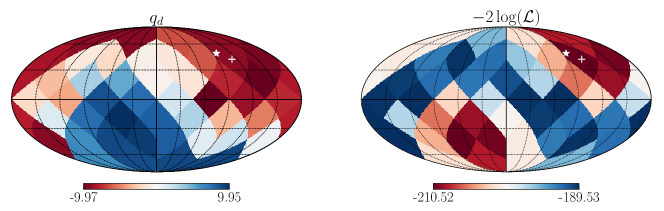
Figure 8: Left: norm of the deceleration dipole vector ${\bf q_{d}}$ as we vary the direction of the dipole to coincide with each HEALPix index shown here. Right: the likelihood of each fit performed here. We show $-2{\rm log}(\mathcal{L})$ for each instance of dipole direction vector. The white star in each panel represents the direction of the CMB dipole, and the white cross is the best-fit direction resulting from this test.

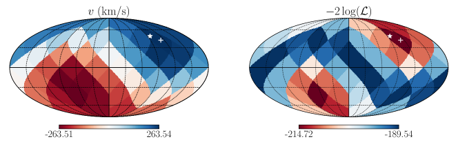
Figure 9: Left: norm of the velocity vector ${\bf v}$ as we vary the direction of the observer boost to coincide with each HEALPix index shown here. Right: the likelihood of each fit performed here. We show $-2{\rm log}(\mathcal{L})$ for each instance of velocity direction. The white star in each panel represents the direction of the CMB dipole, and the white cross is the best-fit direction resulting from this test.

Figure 8 shows the result of our test of the best-fit direction of the dipole in the deceleration parameter, namely, the direction vector associated with ${\bf q_{d}}\equiv q_{d}{\bf n}$ in (11). The left panel shows a Mollweide projection of the best fit amplitude, $q_{d}$, for each corresponding dipole direction, ${\bf n}$. The right panel of Figure 8 shows the corresponding profile log-likelihood function, $-2{\rm log}(\mathcal{L})$, for the direction. The white star on both panels corresponds to the direction of the CMB dipole from Planck Collaboration (2020a), and the white cross is the best-fit direction of our analysis, corresponding to the minimum value of $-2{\rm log}(\mathcal{L})$.

Figure 9 shows the result of our test of the best-fit direction of the observer boost. Specifically, we perform an isotropic cosmological fit with the velocity of the observer, ${\bf v}=v{\bf n}$, left as a free variable. When redshifts are transformed to the CMB frame, ${\bf v}$ is chosen such that the dipole in the CMB temperature field vanishes, while here we leave the best fit rest frame to be determined from the SN Ia catalogue itself. The left panel shows a Mollweide projection of the best fit amplitude of the velocity, $v$, for each corresponding direction ${\bf n}$. The right panel of Figure 9 shows the corresponding profile log-likelihood function for the direction. The white star on both panels again corresponds to the direction of the CMB dipole from Planck Collaboration (2020a), and the white cross is the best-fit direction of our analysis.

The best-fit direction agrees well between the fits for ${\bf q_{d}}$ and ${\bf v}$, with any difference within the angular resolution of our analysis. This shared best fit direction (white cross on all panels) closely coincides with the direction of the CMB dipole (white star on all panels). Colin et al. (2019a) performed this same test for their fits for the dipole in the deceleration parameter, and found their best-fit direction to be $23$°away from the CMB dipole. We find our results to be consistent with that of Colin et al. (2019a) given our resolution.

References

- Andrade et al. (2018) Andrade U., Bengaly C. A. P., Santos B., Alcaniz J. S., 2018, ApJ, 865, 119
- Arendse et al. (2020) Arendse N., et al., 2020, A&A, 639, A57
- Aviles et al. (2014) Aviles A., Bravetti A., Capozziello S., Luongo O., 2014, Phys. Rev. D, 90, 043531
- Bengaly (2016) Bengaly C. A. P. J., 2016, J. Cosmology Astropart. Phys., 2016, 036
- Bengaly et al. (2015) Bengaly C. A. P. J., Bernui A., Alcaniz J. S., 2015, ApJ, 808, 39
- Bernal et al. (2016) Bernal J. L., Verde L., Riess A. G., 2016, J. Cosmology Astropart. Phys., 10, 019
- Betoule et al. (2014) Betoule M., et al., 2014, A&A, 568, A22
- Borderies (2021) Borderies A., 2021, Inhomogeneities and Anisotropies in the Universe analyzed with Supernovae of Type Ia
- Brout et al. (2022) Brout D., et al., 2022, arXiv e-prints, p. arXiv:2202.04077
- Buchert (2000) Buchert T., 2000, Gen. Rel. Grav., 32, 105
- Buchert et al. (2009) Buchert T., Ellis G. F. R., van Elst H., 2009, Gen. Rel. Grav., 41, 2017
- Buchner et al. (2014) Buchner J., et al., 2014, A&A, 564, A125
- Cai & Tuo (2012) Cai R.-G., Tuo Z.-L., 2012, J. Cosmology Astropart. Phys., 2012, 004
- Cattoen & Visser (2007) Cattoen C., Visser M., 2007, Class. Quant. Grav., 24, 5985
- Clarkson & Umeh (2011) Clarkson C., Umeh O., 2011, Class. Quant. Grav., 28, 164010
- Clarkson et al. (2012) Clarkson C., Ellis G. F. R., Faltenbacher A., Maartens R., Umeh O., Uzan J.-P., 2012, Mon. Not. Roy. Astron. Soc., 426, 1121
- Colin et al. (2019a) Colin J., Mohayaee R., Rameez M., Sarkar S., 2019a, arXiv e-prints, p. arXiv:1912.04257
- Colin et al. (2019b) Colin J., Mohayaee R., Rameez M., Sarkar S., 2019b, Astron. Astrophys., 631, L13
- Dam et al. (2017) Dam L. H., Heinesen A., Wiltshire D. L., 2017, Mon. Not. Roy. Astron. Soc., 472, 835
- Dhawan et al. (2022) Dhawan S., et al., 2022, MNRAS, 510, 2228
- Ellis et al. (1985) Ellis G. F. R., Nel S. D., Maartens R., Stoeger W. R., Whitman A. P., 1985, Phys. Rep., 124, 315
- Feeney et al. (2019) Feeney S. M., Peiris H. V., Williamson A. R., Nissanke S. M., Mortlock D. J., Alsing J., Scolnic D., 2019, Phys. Rev. Lett., 122, 061105
- Feroz et al. (2009) Feroz F., Hobson M. P., Bridges M., 2009, MNRAS, 398, 1601
- Freedman (2021) Freedman W. L., 2021, ApJ, 919, 16
- Heinesen (2020) Heinesen A., 2020, arXiv e-prints, p. arxiv:2010.06534
- Heinesen (2021) Heinesen A., 2021, Phys. Rev. D, 104, 123527
- Heinesen & Macpherson (2022) Heinesen A., Macpherson H. J., 2022, J. Cosmology Astropart. Phys., 2022, 057
- Hogg et al. (2005) Hogg D. W., Eisenstein D. J., Blanton M. R., Bahcall N. A., Brinkmann J., Gunn J. E., Schneider D. P., 2005, Astrophys. J., 624, 54
- Horstmann et al. (2021) Horstmann N., Pietschke Y., Schwarz D. J., 2021, arXiv e-prints, p. arXiv:2111.03055
- Hutsemékers et al. (2005) Hutsemékers D., Cabanac R., Lamy H., Sluse D., 2005, A&A, 441, 915
- Hutsemékers et al. (2014) Hutsemékers D., Braibant L., Pelgrims V., Sluse D., 2014, A&A, 572, A18
- Jones et al. (2021) Jones D. O., et al., 2021, ApJ, 908, 143
- Kalus et al. (2013) Kalus B., Schwarz D. J., Seikel M., Wiegand A., 2013, A&A, 553, A56
- Kristian & Sachs (1966) Kristian J., Sachs R. K., 1966, ApJ, 143, 379
- Laurent et al. (2016) Laurent P., et al., 2016, JCAP, 11, 060
- Leibundgut & Sullivan (2018) Leibundgut B., Sullivan M., 2018, Space Sci. Rev., 214, 57
- Lemos et al. (2019) Lemos P., Lee E., Efstathiou G., Gratton S., 2019, MNRAS, 483, 4803
- MacCallum & Ellis (1970) MacCallum M. A. H., Ellis G. F. R., 1970, Comm. Math. Phys., 19, 31
- Macaulay et al. (2019) Macaulay E., et al., 2019, MNRAS, 486, 2184
- Macpherson & Heinesen (2021) Macpherson H. J., Heinesen A., 2021, Phys. Rev. D, 104, 023525
- Migkas et al. (2021) Migkas K., Pacaud F., Schellenberger G., Erler J., Nguyen-Dang N. T., Reiprich T. H., Ramos-Ceja M. E., Lovisari L., 2021, Astron. Astrophys., 649, A151
- Nielsen et al. (2016) Nielsen J. T., Guffanti A., Sarkar S., 2016, Sci. Rep., 6, 35596