Surface energy coefficient of a N2LO Skyrme energy functional : a semiclassical Extended Thomas-Fermi approach

Abstract

We generalize to N2LO Skyrme functionals the semi-classical approach of Grammaticos and Voros [1, 2] in order to calculate the Extended Thomas Fermi expressions of the new densities and currents appearing at the N2LO level. Within a one dimensional symmetric semi infinite nuclear matter model and using a simple Fermi-like density profile, we obtain an easy-to-use formula for the surface energy including the contributions of the central, density-dependent and spin-orbit terms up to $\hbar^{2}$. Such a formula can be easily used as a first attempt to constrain the surface properties of new N2LO Skyrme parametrizations. The N2LO parametrization tested in this paper is shown to exhibit a shift (compared to a full Hartree-Fock calculation) which is quantitatively similar to the one obtained with the traditional Skyrme parametrizations.

I Introduction

Microscopic self-consistent models based on the mean field approximation have demonstrated their usefulness to describe precisely a wide range of nuclear properties such as binding energies, radii, separation energies, energy spectra or also fission barriers of heavy nuclei. At this time, they even allow rather pertinent analysis of spectroscopy of superheavy nuclei for which there exists a lot of recent experimental results. All these models use as a basic ingredient an effective interaction containing parameters which must be determined from a panel of pseudo and experimental data within a precise protocol. Among the pseudo data used in the fitting procedure, properties of infinite matter are usually incorporated but those of semi-infinite nuclear matter are often neglected because of the required computational time. However, the surface energy has been recognized in the early years as one of the fundamental properties of nuclei and thus entered the liquid drop formula even in its simplest form. In this particular formula, its role is to keep a nucleus spherical (against Coulomb repulsion for instance) but more generally, its physical meaning is related to the shape of a nucleus and its ability to deform. From a fundamental point of view, since this last property is controlled by the compressibility for small density oscillations, both quantities are related [3, 4]. From a practical point of view, the surface energy naturally contributes to the deformation properties of nuclei [5, 6] and thus in fusion reactions [7, 8, 9, 10, 11], to the determination of fission barriers [12, 13] or in cluster decay [14] and neutron-star matter [15]. It is therefore of the utmost importance to determine precisely the surface energy and each of the aforementionned constraints could be used to fine tune the parameters of an effective interaction [5, 16, 17]. Historically, this was not the case and the huge difference between the result obtained with a Skyrme parametrization and the experimental fission barrier height of ²⁴⁰Pu induced the adjustment of SkM* [5]. This parametrization is a modified version of SkM [18] fine tuned in such a way that the height of a semi classical calculation of the fission barrier [19] is well reproduced without any modification of infinite nuclear matter isoscalar properties. The parametrization SkM* is still quite commonly used for the description of fission phenomena [20].

Since neither the fission barriers neither a full Hartree-Fock (HF) calculation of the surface energy [21] can be directly used in a fitting protocol because of the numerical cost, semi-classical methods and especially the Extended Thomas Fermi (ETF) expansion method [22, 23, 24, 1, 2, 19] were developed as an alternative. This kind of approach is of great interest when one is concerned by an approximation of the total energy of a fermionic system, let us say a nucleus made with neutrons and protons, but not by an approximation of the total wave function. Generally speaking, semi classical methods are mainly based on the Strutinsky theorem, such that one can split the Hartree-Fock energy of a system of fermions in two parts: an important smoothly varying part which can be roughly described by the liquid drop model, plus a smaller, but not smooth, part purely related to shell effects [25, 26, 27, 28, 29]. Semi-classical expansions are actually known to give an accurate description of the smooth part of the energy. Practically speaking, they consist of an expansion in powers of $\hbar$ of the density matrix which allows us to express each of the densities and currents appearing in the energy density functional as functions of the Fermi modulus $k_{F}$, the effective mass field $f$ and their spatial derivatives. Then, by eliminating $k_{F}$, one can express the energy with respect to the density and it’s spatial derivatives alone. The great advantage comes from the variational principle with respect to the individual wave functions which is replaced by a simpler variational principle with respect to the density profile itself. This leads to an easy-to-use formula which reduces drastically the computer time when compared to microscopic HF calculations. Two methods have been used in the past to obtain an ETF expansion. First an expansion in powers of $\hbar$ of the Bloch density [22, 23, 24, 19] and second the Wigner-Kirkwood transform of a one-body hamiltonian [1, 2]. A direct and recent application of this approach can be found in Jodon et al. [30] and in Ryssens et al. [6] where the authors examined the correlation between the surface energy and the deformation properties of heavy nuclei. In Jodon et al. [30] in particular, the authors revisited a very simple ETF expansion obtained by Krivine and Treiner [31, 32] in order to obtain a simple formula for the surface energy and thus to obtain an easy-to-implement constraint in the fitting procedure which leads to the so-called SLy5s parametrizations [30]. In this work, we extend the method developed by Grammaticos and Voros [1, 2] to Skyrme energy density functional (EDF) containing 4th gradient terms (named N2LO) which are expected to improve the calculated properties of nuclei [33]. Temperature effects, relativistic models as well as the possibility of superfluidity are not been considered here. The paper is organized as follows. Section II recalls the N2LO Skyrme EDF considered here. Section III generalizes the results obtained in [1, 2] for the new densities appearing at the N2LO order. Section IV uses the semi-classical ETF results of the third section to calculate the surface energy of a N2LO Skyrme functional within a 1D semi-infinite nuclear matter model. Section V presents the discussion of our results.

II The Skyrme Energy Density Functional at the N2LO order

II.1 Local densities and currents

The interaction used in this paper is the so-called N2LO extension [34, 35, 36, 37] of the traditional Skyrme interaction. It implies gradients up to fourth order. In Ref.[38], the authors considered specific densities more suited to 3D HF numerical calculations but for this formal work, we keep here the more compact notations for densities introduced in [39]. The density matrix elements (the $q$-index is for the n/p representation) in direct and spin spaces reads:

$$\langle\bm{\mathbf{r}}\sigma|\hat{\rho}_{q}|\bm{\mathbf{r}}^{\prime}\sigma^{\prime}\rangle = \rho_{q}(\bm{\mathbf{r}}\sigma,\bm{\mathbf{r}}^{\prime}\sigma^{\prime})\,=\,\frac{1}{2}\,\rho_{q}(\bm{\mathbf{r}},\bm{\mathbf{r}}^{\prime})\,\delta_{\sigma\sigma^{\prime}}\,+\,\frac{1}{2}\,\bm{\mathbf{s}}_{q}(\bm{\mathbf{r}},\bm{\mathbf{r}}^{\prime})\,\langle\sigma|\hat{\bm{\mathbf{\sigma}}}|\sigma^{\prime}\rangle\,=\,\langle\bm{\mathbf{r}}\sigma|\frac{\hat{\rho}_{q,\bm{\mathbf{r}}}\otimes\hat{\mathbb{1}}_{\sigma}\,+\,\hat{\bm{\mathbf{s}}}_{q,\bm{\mathbf{r}}}\otimes\hat{\bm{\mathbf{\sigma}}}}{2}|\bm{\mathbf{r}}^{\prime}\sigma^{\prime}\rangle\quad,$$ (1)

where

$$\hat{\rho}_{q,\bm{\mathbf{r}}} = \rm Tr_{\sigma}(\hat{\rho}_{q})\quad,$$ (2a)

$$\hat{\bm{\mathbf{s}}}_{q,\bm{\mathbf{r}}} = \rm Tr_{\sigma}(\hat{\rho}_{q}\hat{\bm{\mathbf{\sigma}}})\quad.$$ (2b)

We introduce now the useful local densities as:

$$\rho_{q}(\bm{\mathbf{r}}) = \,\rho_{q}(\bm{\mathbf{r}},\bm{\mathbf{r}}^{\prime})\big{|}_{\bm{\mathbf{r}}=\bm{\mathbf{r}}^{\prime}}\quad,$$ (3a)

$$\bm{\mathbf{s}}_{q}(\bm{\mathbf{r}}) = \,\bm{\mathbf{s}}_{q}(\bm{\mathbf{r}},\bm{\mathbf{r}}^{\prime})\big{|}_{\bm{\mathbf{r}}=\bm{\mathbf{r}}^{\prime}}\quad,$$ (3b)

$$\tau_{q}(\bm{\mathbf{r}}) = \,\bm{\mathbf{\nabla}}\cdot\bm{\mathbf{\nabla}}^{\prime}\;\rho_{q}(\bm{\mathbf{r}},\bm{\mathbf{r}^{\prime}})\big{|}_{\bm{\mathbf{r}}=\bm{\mathbf{r}^{\prime}}}\quad,$$ (3c)

$$\tau_{q,\mu\nu}^{(s)}(\bm{\mathbf{r}}) = \,\frac{1}{2}\,\big{(}\nabla_{\mu}\nabla_{\nu}^{\prime}+\nabla_{\nu}\nabla_{\mu}^{\prime}\big{)}\,\rho_{q}(\bm{\mathbf{r}},\bm{\mathbf{r}^{\prime}})\big{|}_{\bm{\mathbf{r}}=\bm{\mathbf{r}^{\prime}}}\quad,$$ (3d)

$$Q_{q}(\bm{\mathbf{r}}) = \,\Delta\Delta^{\prime}\rho_{q}(\bm{\mathbf{r}},\bm{\mathbf{r}^{\prime}})\big{|}_{\bm{\mathbf{r}}=\bm{\mathbf{r}^{\prime}}}\quad,$$ (3e)

$$J_{q,\mu\nu}(\bm{\mathbf{r}}) = \frac{1}{2i}\,\big{(}\nabla_{\mu}-\nabla_{\mu}^{\prime}\big{)}\,s_{\nu,q}(\bm{\mathbf{r}},\bm{\mathbf{r}}^{\prime})\big{|}_{\bm{\mathbf{r}}=\bm{\mathbf{r}}^{\prime}}\quad,$$ (3f)

$$C_{q,\mu\nu}(\bm{\mathbf{r}}) = \,\frac{1}{2i}\,\big{(}\,\Delta^{\prime}\nabla_{\mu}-\Delta\nabla_{\mu}^{\prime}\,\big{)}\,s_{\nu}(\bm{\mathbf{r}},\bm{\mathbf{r}}^{\prime})\big{|}_{\bm{\mathbf{r}}=\bm{\mathbf{r}}^{\prime}}\quad.$$ (3g)

Time reversal invariance is assumed which restrict our work to even-even nuclei or unpolarized infinite systems. Using this assumption, the time odd part of the Skyrme EDF vanishes so that the corresponding densities do not appear in the list above. The treatment of the time odd part of the NLO part of the Skyrme EDF has been made by Grammaticos and Voros in [1]. It requires the definition of the corresponding currents but does not imply any specific issues and will be treated in future developments.

II.2 The Skyrme EDF

We consider in this paper a Skyrme pseudo potential containing a 2-body central (C) term and a spin-orbit (SO) term up to NLO order (see Ref.[40] for notations) plus a central N2LO component as developed in [33]. Let us note that the tensor (T) part of two body pseudo-potentials as developed in [41] could be also introduced without major changes since the spin-gradient coupling present in the C part already generates a tensor component in the Skyrme EDF (see the expression of $\mathcal{H}^{\rm NLO}_{\rm T}$, Eq. (4a) below). Similarly, the central three body part developed in [42, 43] could be also taken into account by a modification of the concerned one body fields.

Finally, we can write the functional as (the $q=n/p$ refers to the neutron/proton representation while the $t=0,1$ index refers to the isoscalar/isovector representation):

$$\mathcal{H} = \,\mathcal{H}^{\rm LO}_{\rm C}\,+\,\mathcal{H}^{\rm NLO}_{\rm C}\,+\,\mathcal{H}^{\rm NLO}_{\rm SO}\,+\,\mathcal{H}^{\rm NLO}_{\rm T}\,+\,\mathcal{H}^{\rm N2LO}_{\rm C}\,+\,\mathcal{H}^{\rm N2LO}_{\rm T}\quad,$$ (4a)

$$\mathcal{H}^{\rm LO}_{\rm C} = \,\sum_{t=0,1}\,C_{t}^{\rho}\left[\rho_{0}\right]\,\rho_{t}^{2}\,=\,\sum_{t=0,1}\,\left[\,C_{t}^{\rho}\,+\,C_{t}^{\rho^{\gamma}}\,\rho_{0}^{\gamma}\right]\,\rho_{t}^{2}\quad,$$ (4b)

$$\mathcal{H}^{\rm NLO}_{\rm C} = \,\sum_{t=0,1}\,C_{t}^{\Delta\rho}\,\rho_{t}\,\Delta\rho_{t}\,+\,C_{t}^{\tau}\,\rho_{t}\,\tau_{t}\quad,$$ (4c)

$$\mathcal{H}^{\rm NLO}_{\rm T} = \,-\,\frac{1}{2}\,\sum_{t=0,1}\,C_{t}^{T}\,\bm{\mathbf{J}}_{t}^{2}\quad,$$ (4d)

$$\mathcal{H}^{\rm NLO}_{\rm SO} = \,\sum_{t=0,1}\,C_{t}^{\nabla J}\,\rho_{t}\,\left(\bm{\mathbf{\nabla}}\cdot\bm{\mathbf{J}}_{t}\right)\quad,$$ (4e)

$$\mathcal{H}^{\rm N2LO}_{\rm C} = \,\sum_{t=0,1}\,C_{t}^{(\Delta\rho)^{2}}\,\left(\Delta\rho_{t}\right)^{2}\,+\,C_{t}^{M\rho}\,\Big{[}\,\rho_{t}\,Q_{t}\,+\,\tau_{t}^{2}\,+\,2\,\left(\,\tau^{(s)}_{t,\mu\nu}\tau^{(s)}_{t,\mu\nu}\,-\,\tau^{(s)}_{t,\mu\nu}\,\nabla_{\mu}\nabla_{\nu}\rho\,\right)\,\Big{]}\quad,$$ (4f)

$$\mathcal{H}^{\rm N2LO}_{\rm T} = \,\sum_{t=0,1}\,C_{t}^{MT}\,\Big{[}\,2\,\bm{\mathbf{J}}_{t}\cdot\bm{\mathbf{C}}_{t}\,-\,\frac{1}{2}\bm{\mathbf{J}}_{t}\cdot\Delta\bm{\mathbf{J}}_{t}\,\Big{]}\quad,$$ (4g)

where $\bm{\mathbf{J}}_{t}$ and $\bm{\mathbf{C}}_{t}$ are the vector components of $J_{t,\mu\nu}$ and $C_{t,\mu\nu}$ respectively and where the repeated $\mu,\nu$ indexes are summed over the cartesian coordinates. At this stage, we made a second assumption which induced the reduction of the tensor currents to their vector part. This occurs in spherical nuclei and also in semi infinite nuclear matter as we will see in a further section.

II.3 The one body hamiltonian

The one body hamiltonian associated to the above N2LO EDF is given by:

$$h_{q}(\bm{\mathbf{r}}\sigma,\bm{\mathbf{r}}^{\prime}\sigma^{\prime}) = \,\langle\bm{\mathbf{r}}\sigma|\hat{h}_{q}|\bm{\mathbf{r}}^{\prime}\sigma^{\prime}\rangle\,=\,\frac{\delta E}{\delta\rho_{q}(\bm{\mathbf{r}}^{\prime}\sigma^{\prime},\bm{\mathbf{r}}\sigma)}\,=\,\frac{\delta}{\delta\rho_{q}(\bm{\mathbf{r}}^{\prime}\sigma^{\prime},\bm{\mathbf{r}}\sigma)}\,\int_{\mathbb{R}^{3}}\,d^{3}\bm{\mathbf{r}}^{\prime\prime}\,\mathcal{H}(\bm{\mathbf{r}}^{\prime\prime})$$ (5)

$$= \,U_{q}(\bm{\mathbf{r}})\,\delta(\bm{\mathbf{r}}-\bm{\mathbf{r}}^{\prime})\,\delta_{\sigma\sigma^{\prime}}\,-\,\nabla_{\mu}\bigg{[}\,B_{q,\mu\nu}(\bm{\mathbf{r}})\nabla_{\nu}\delta(\bm{\mathbf{r}}-\bm{\mathbf{r}}^{\prime})\,\bigg{]}\,\delta_{\sigma\sigma^{\prime}}\,+\,\Delta\bigg{[}\,D_{q}(\bm{\mathbf{r}})\Delta\delta(\bm{\mathbf{r}}-\bm{\mathbf{r}}^{\prime})\,\bigg{]}\,\delta_{\sigma\sigma^{\prime}}$$

$$\,+\,i\,\bm{\mathbf{W}}_{q}(\bm{\mathbf{r}})\cdot\bigg{(}\langle\sigma|\hat{\bm{\mathbf{\sigma}}}|\sigma^{\prime}\rangle\times\bm{\mathbf{\nabla}}\delta(\bm{\mathbf{r}}-\bm{\mathbf{r}}^{\prime})\bigg{)}\,+\,i\,\bm{\mathbf{\nabla}}\cdot\bigg{[}\,\left[\,\bm{\mathbf{V}}_{q}(\bm{\mathbf{r}})\cdot\left(\langle\sigma|\hat{\bm{\mathbf{\sigma}}}|\sigma^{\prime}\rangle\times\bm{\mathbf{\nabla}}\right)\,\right]\,\bm{\mathbf{\nabla}}\delta(\bm{\mathbf{r}}-\bm{\mathbf{r}}^{\prime})\bigg{]}\quad,$$

where the fields can be separated in their NLO+N2LO components as

$$U_{q}(\bm{\mathbf{r}}) = \,U_{q}^{\text{NLO}}(\bm{\mathbf{r}})\,+\,U_{q}^{\text{N2LO}}(\bm{\mathbf{r}})\quad,$$ (6a)

$$B_{q,\mu\nu}(\bm{\mathbf{r}}) = \,B_{q}^{\text{NLO}}(\bm{\mathbf{r}})\,\delta_{\mu\nu}\,+\,B_{q,\mu\nu}^{\text{N2LO}}(\bm{\mathbf{r}})\quad,$$ (6b)

$$D_{q}(\bm{\mathbf{r}}) = \,D_{q}^{\text{N2LO}}(\bm{\mathbf{r}})\quad,$$ (6c)

$$\bm{\mathbf{W}}_{q}(\bm{\mathbf{r}}) = \,\bm{\mathbf{W}}_{q}^{\text{NLO}}(\bm{\mathbf{r}})\,+\,\bm{\mathbf{W}}_{q}^{\text{N2LO}}(\bm{\mathbf{r}})\quad,$$ (6d)

$$\bm{\mathbf{V}}_{q}(\bm{\mathbf{r}}) = \,\bm{\mathbf{V}}_{q}^{\text{N2LO}}(\bm{\mathbf{r}})\quad.$$ (6e)

The expressions of all the above fields in terms of densities and currents are given in Appendix A. At the N2LO order two new fields appear, i.e. $D_{q}(\bm{\mathbf{r}})$ and $\bm{\mathbf{V}}_{q}(\bm{\mathbf{r}})$. Moreover, $B_{q}(\bm{\mathbf{r}})$ field is no longer a scalar (as for NLO) but now becomes a symmetric rank 2 tensor with a non-zero contribution of its scalar part and its deviator (i.e. symmetric and traceless) part.

III The semi classical Extended Thomas Fermi approximation

III.1 The Wigner-Kirkwood transform

We now focus on the semi-classical expansion of the N2LO functional and follow the notations of Grammaticos and Voros [1, 2]. The Wigner-Kirkwood transform of an operator $\hat{A}$ and of a product of operators $\hat{A}\hat{B}$ are respectively given by [44]:

$$A_{\scriptscriptstyle W}(\bm{\mathbf{R}},\bm{\mathbf{p}},\hbar)=\int_{\mathbb{R}^{3}}d^{3}{\bf r}\ \langle\bm{\mathbf{R}}-\tfrac{1}{2}\bm{\mathbf{r}}|\hat{A}(\hbar)|\bm{\mathbf{R}}+\tfrac{1}{2}\bm{\mathbf{r}}\rangle e^{i\bm{\mathbf{p}}\bm{\mathbf{r}}/\hbar}$$ (7)

and [45]

$$(\hat{A}\hat{B})_{\scriptscriptstyle W}=A_{\scriptscriptstyle W}e^{\frac{1}{2}i\hbar\overleftrightarrow{\Lambda}}B_{\scriptscriptstyle W}$$ (8)

with

$$\overleftrightarrow{\Lambda}\equiv\sum_{i}\left(\frac{\overleftarrow{\partial}}{\partial r_{i}}\frac{\overrightarrow{\partial}}{\partial p_{i}}-\frac{\overleftarrow{\partial}}{\partial p_{i}}\frac{\overrightarrow{\partial}}{\partial r_{i}}\right)$$ (9)

where the above operator acts on left or right side depending on the arrows. The object of interest we want to expand in powers of $\hbar$ is the density matrix which, at zero temperature, reads :

$$\hat{\rho}_{q}=\Theta(E_{F,q}\,\hat{\mathbb{1}}_{\bm{\mathbf{r}}\otimes\sigma}-\hat{h}_{q})$$ (10)

where $\hat{h}_{q}$ is the one-body hamiltonian and $E_{F,q}$ the Fermi energy of species $q$. Since we consider the case with a spin-orbit term, the Wigner transform of $\hat{h}_{q}$ can thus be expressed as (${\bf x}\equiv({\bf R},\bm{\mathbf{p}})$):

$$(\hat{h}_{q})_{\scriptscriptstyle W}({\bf x},\hbar)=H_{q,cl}({\bf R},\bm{\mathbf{p}})\hat{\mathbb{1}}_{\sigma}+\hbar\,{\bf H_{q,so}}({\bf R},\bm{\mathbf{p}})\cdot\hat{\bm{\mathbf{\sigma}}}$$ (11)

where $H_{q,cl}$ represents the classical limit (obtained formally when $\hbar$ goes to zero) and ${\bf H_{q,so}}$ the spin-orbit part, which enters the expansion as a first-order $\hbar$ correction (see Ref.[2]). Given any analytical functions $F$ of the hamiltonian $\hat{h}_{q}$, the expansion in the vicinity of its classical value reads:

$$F(\hat{h}_{q})=\sum_{n}^{\infty}\frac{1}{n!}F^{(n)}(H_{q,cl}({\bf x}))(\hat{h}_{q}-H_{q,cl}({\bf x})\hat{\mathbb{1}}_{\bm{\mathbf{r}}\otimes\sigma})^{n}$$ (12)

so that the Wigner-Kirkwood transform is

$$(F(\hat{h}_{q}))_{\scriptscriptstyle W}({\bf x},\hbar)=\sum_{n}^{\infty}\frac{1}{n!}F^{(n)}(H_{q,cl}({\bf x}))\hat{\cal G}_{q,n}({\bf x},\hbar)$$ (13)

with

$$\hat{\cal G}_{q,n}({\bf x},\hbar)=\left.((\hat{h}_{q}-H_{q,cl}({\bf x})\hat{\mathbb{1}}_{\bm{\mathbf{r}}\otimes\sigma})^{n})_{\scriptscriptstyle W}({\bf x}^{\prime},\hbar)\right|_{{\bf x}^{\prime}={\bf x}}$$ (14)

which are universal operators for a given Hamiltonian, i.e. independent of the function $F$. At order $\hbar^{3}$, we recover the results of Grammaticos and Voros [2] :

$$\hat{\cal G}_{q,0}({\bf x},\hbar) = \,\hat{\mathbb{1}}_{\sigma}$$

$$\hat{\cal G}_{q,1}({\bf x},\hbar) = \,\hbar\,{\bf H_{q,so}}\cdot\hat{\bm{\mathbf{\sigma}}}$$

$$\hat{\cal G}_{q,2}({\bf x},\hbar) = \,\frac{\hbar^{2}}{4}\,\big{[}\,4\,{\bf H_{q,so}}^{2}\,+\,(\partial^{2}_{x_{\mu}p_{\nu}}H_{q,cl})\,(\partial^{2}_{x_{\nu}p_{\mu}}H_{q,cl})\,-\,(\partial^{2}_{x_{\mu}x_{\nu}}H_{q,cl})\,(\partial^{2}_{p_{\mu}p_{\nu}}H_{q,cl})\,\big{]}\,\hat{\mathbb{1}}_{\sigma}\,+\,{\cal O}(\hbar^{3})$$

$$\hat{\cal G}_{q,3}({\bf x},\hbar) = \,\frac{\hbar^{2}}{4}\,\big{[}\,2\,(\partial^{2}_{x_{\mu}p_{\nu}}H_{q,cl})\,(\partial_{p_{\mu}}H_{q,cl})\,(\partial_{x_{\nu}}H_{q,cl})\,-\,(\partial^{2}_{x_{\mu}x_{\nu}}H_{q,cl})\,(\partial_{p_{\mu}}H_{q,cl})\,(\partial_{p_{\nu}}H_{q,cl})$$

$$\hskip 170.71652pt\,-\,(\partial^{2}_{p_{\mu}p_{\nu}}H_{q,cl})\,(\partial_{x_{\mu}}H_{q,cl})\,(\partial_{x_{\nu}}H_{q,cl})\,\big{]}\,\hat{\mathbb{1}}_{\sigma}\,+\,{\cal O}(\hbar^{3})$$

We thus immediately obtain for the density matrix :

$$(\hat{\rho_{q}})_{\scriptscriptstyle W}(\bm{\mathbf{r}},\bm{\mathbf{p}}) = \,\Theta(E_{F,q}-H_{q,cl}(\bm{\mathbf{r}},\bm{\mathbf{p}}))\,\hat{\mathbb{1}}_{\sigma}\,-\,\sum_{n=1}^{\infty}\,\frac{\hat{\cal G}_{q,n}({\bf x},\hbar)}{n!}\,\delta^{(n-1)}\,(H_{q,cl}(\bm{\mathbf{r}},\bm{\mathbf{p}})-E_{F,q})$$

and the non zero densities and currents read

$$\rho_{q}(\bm{\mathbf{r}}) = \,\int_{\mathbb{R}^{3}}\frac{d^{3}{\bf p}}{(2\pi\hbar)^{3}}\,(\hat{\rho}_{q,\bm{\mathbf{r}}})_{\scriptscriptstyle W}(\bm{\mathbf{r}},\bm{\mathbf{p}})\quad,$$ (15)

$$\tau_{q}(\bm{\mathbf{r}}) = \,\frac{1}{4}\,\Delta\,\int_{\mathbb{R}^{3}}\frac{d^{3}{\bf p}}{(2\pi\hbar)^{3}}\,(\hat{\rho}_{q,\bm{\mathbf{r}}})_{\scriptscriptstyle W}(\bm{\mathbf{r}},\bm{\mathbf{p}})\,+\,\int_{\mathbb{R}^{3}}\frac{d^{3}{\bf p}}{(2\pi\hbar)^{3}}\,\frac{p^{2}}{\hbar^{2}}\,(\hat{\rho}_{q,\bm{\mathbf{r}}})_{\scriptscriptstyle W}(\bm{\mathbf{r}},\bm{\mathbf{p}})\quad,$$ (16)

$$\tau_{q,\mu\nu}^{(s)}(\bm{\mathbf{r}}) = \,\frac{1}{4}\,\nabla_{\mu}\nabla_{\nu}\,\int_{\mathbb{R}^{3}}\frac{d^{3}{\bf p}}{(2\pi\hbar)^{3}}\,(\hat{\rho}_{q,\bm{\mathbf{r}}})_{\scriptscriptstyle W}(\bm{\mathbf{r}},\bm{\mathbf{p}})\,+\,\int_{\mathbb{R}^{3}}\frac{d^{3}{\bf p}}{(2\pi\hbar)^{3}}\,\frac{p_{\mu}p_{\nu}}{\hbar^{2}}\,(\hat{\rho}_{q,\bm{\mathbf{r}}})_{\scriptscriptstyle W}(\bm{\mathbf{r}},\bm{\mathbf{p}})\quad,$$ (17)

$$Q_{q}(\bm{\mathbf{r}}) = \,\frac{1}{16}\,\Delta\Delta\,\int_{\mathbb{R}^{3}}\frac{d^{3}{\bf p}}{(2\pi\hbar)^{3}}\,(\hat{\rho}_{q,\bm{\mathbf{r}}})_{\scriptscriptstyle W}(\bm{\mathbf{r}},\bm{\mathbf{p}})\,+\,\int_{\mathbb{R}^{3}}\frac{d^{3}{\bf p}}{(2\pi\hbar)^{3}}\,\frac{p^{4}}{\hbar^{4}}\,(\hat{\rho}_{q,\bm{\mathbf{r}}})_{\scriptscriptstyle W}(\bm{\mathbf{r}},\bm{\mathbf{p}})\,-\,\frac{1}{2}\,\Delta\,\int_{\mathbb{R}^{3}}\frac{d^{3}{\bf p}}{(2\pi\hbar)^{3}}\,\frac{p^{2}}{\hbar^{2}}\,(\hat{\rho}_{q,\bm{\mathbf{r}}})_{\scriptscriptstyle W}(\bm{\mathbf{r}},\bm{\mathbf{p}})$$ (18)

$$\hskip 227.62204pt+\,\int_{\mathbb{R}^{3}}\frac{d^{3}{\bf p}}{(2\pi\hbar)^{3}}\,\frac{(\bm{\mathbf{p}}\cdot\bm{\mathbf{\nabla}})^{2}}{\hbar^{2}}\,(\hat{\rho}_{q,\bm{\mathbf{r}}})_{\scriptscriptstyle W}(\bm{\mathbf{r}},\bm{\mathbf{p}})\quad,$$

$$J_{q,\mu\nu}(\bm{\mathbf{r}}) = \,\int_{\mathbb{R}^{3}}\frac{d^{3}{\bf p}}{(2\pi\hbar)^{3}}\,\frac{p_{\mu}}{\hbar}\,(\hat{s}_{q,\bm{\mathbf{r}},\nu})_{W}(\bm{\mathbf{r}},\bm{\mathbf{p}})\quad,$$ (19)

$$C_{q,\mu\nu}(\bm{\mathbf{r}}) = \,\frac{1}{4}\,\Delta\int_{\mathbb{R}^{3}}\frac{d^{3}{\bf p}}{(2\pi\hbar)^{3}}\,\frac{p_{\mu}}{\hbar}\,(\hat{s}_{q,\bm{\mathbf{r}},\nu})_{W}(\bm{\mathbf{r}},\bm{\mathbf{p}})\,-\,\int_{\mathbb{R}^{3}}\frac{d^{3}{\bf p}}{(2\pi\hbar)^{3}}\,\frac{\bm{\mathbf{p}}^{2}}{\hbar^{2}}\,\frac{p_{\mu}}{\hbar}\,(\hat{s}_{q,\bm{\mathbf{r}},\nu})_{W}(\bm{\mathbf{r}},\bm{\mathbf{p}})$$ (20)

$$\hskip 227.62204pt-\,\frac{1}{2}\,\nabla_{\mu}\int_{\mathbb{R}^{3}}\frac{d^{3}{\bf p}}{(2\pi\hbar)^{3}}\,\frac{(\bm{\mathbf{p}}\cdot\bm{\mathbf{\nabla}})}{\hbar}\,(\hat{s}_{q,\bm{\mathbf{r}},\nu})_{W}(\bm{\mathbf{r}},\bm{\mathbf{p}})\quad,$$

with

$$(\hat{\rho}_{q,\bm{\mathbf{r}}})_{\scriptscriptstyle W}(\bm{\mathbf{r}},\bm{\mathbf{p}}) =\rm Tr_{\sigma}[(\hat{\rho}_{q})_{\scriptscriptstyle W}(\bm{\mathbf{r}},\bm{\mathbf{p}})]\quad,$$

$$(\hat{\bm{\mathbf{s}}}_{q,\bm{\mathbf{r}}})_{\scriptscriptstyle W}(\bm{\mathbf{r}},\bm{\mathbf{p}}) =\rm Tr_{\sigma}[(\hat{\rho}_{q})_{\scriptscriptstyle W}(\bm{\mathbf{r}},\bm{\mathbf{p}})\ \hat{\bm{\mathbf{\sigma}}}]\quad.$$

If $H_{q,cl}$ is invariant under rotations in momentum space, the above expressions can be simplified since the angular average can be done explicitly. By instance, we define, following Ref.[1]

$$\hat{\alpha}_{q,k}(\bm{\mathbf{r}})=\int_{0}^{\infty}dp\ p^{k-1-n}\bigg{\langle}(\hat{\rho}_{q,\bm{\mathbf{r}}})_{\scriptscriptstyle W}(\bm{\mathbf{r}},\bm{\mathbf{p}})\bigg{\rangle}\quad,$$ (21)

where $\langle f({\bf r},{\bf p})\rangle=\frac{1}{4\pi}\int_{S^{2}}d^{2}(\frac{{\bf p}}{p})\ f({\bf r},{\bf p})$ is the momentum angular average over the unit 2-sphere $S^{2}$. Taking $H_{q,cl}$ as the new integration variable , we can then write

$$\hat{\alpha}_{q,k}(\bm{\mathbf{r}})=\frac{p_{F}^{k}}{k}\mathbb{1}_{\sigma}-\sum_{r=1}^{\infty}\frac{1}{r!}\left[\left(-\frac{1}{\frac{\partial H_{q,cl}}{\partial p}}\frac{\partial}{\partial p}\right)^{r-1}\left(\frac{p^{k-1}}{{\frac{\partial H_{q,cl}}{\partial p}}}\langle{\cal\hat{G}}_{q,r}\rangle\right)\right]\Bigg{|}_{p=p_{F}(\bm{\mathbf{r}})}$$ (22)

Because of the spin-orbit and N2LO terms, we also need

$$\hat{\alpha}_{q,k,\mu}(\bm{\mathbf{r}})=-\sum_{r=1}^{\infty}\frac{1}{r!}\left[\left(-\frac{1}{\frac{\partial H_{q,cl}}{\partial p}}\frac{\partial}{\partial p}\right)^{r-1}\left(\frac{p^{k-2}}{\frac{\partial H_{q,cl}}{\partial p}}\langle{p_{\mu}\;\cal\hat{G}}_{q,r}\rangle\right)\right]\Bigg{|}_{p=p_{F}(\bm{\mathbf{r}})}$$ (23)

$$\hat{\alpha}_{q,k,\mu\nu}(\bm{\mathbf{r}})=\frac{p_{F}^{k}}{3k}\mathbb{1}_{\sigma}\delta_{\mu\nu}-\sum_{r=1}^{\infty}\frac{1}{r!}\left[\left(-\frac{1}{\frac{\partial H_{q,cl}}{\partial p}}\frac{\partial}{\partial p}\right)^{r-1}\left(\frac{p^{k-3}}{\frac{\partial H_{q,cl}}{\partial p}}\langle{p_{\mu}p_{\nu}\;\cal\hat{G}}_{q,r}\rangle\right)\right]\Bigg{|}_{p=p_{F}(\bm{\mathbf{r}})}$$ (24)

We can thus write

$$\rho_{q}(\bm{\mathbf{r}}) = \,\frac{\rm Tr_{\sigma}(\hat{\alpha}_{q,3})}{2\pi^{2}\hbar^{3}}\quad,$$ (25a)

$$\tau_{q}(\bm{\mathbf{r}}) = \,\frac{\Delta\rm Tr_{\sigma}(\hat{\alpha}_{q,3})}{8\pi^{2}\hbar^{3}}\,+\,\frac{\rm Tr_{\sigma}(\hat{\alpha}_{q,5})}{2\pi^{2}\hbar^{5}}\quad,$$ (25b)

$$\tau_{q,\mu\nu}^{(s)}(\bm{\mathbf{r}}) = \,\frac{\nabla_{\mu}\nabla_{\nu}\rm Tr_{\sigma}(\hat{\alpha}_{q,3})}{8\pi^{2}\hbar^{3}}\,+\,\frac{\rm Tr_{\sigma}(\hat{\alpha}_{q,5,\mu\nu})}{2\pi^{2}\hbar^{5}}\quad,$$ (25c)

$$Q_{q}(\bm{\mathbf{r}}) = \,\frac{\Delta^{2}\rm Tr_{\sigma}(\hat{\alpha}_{q,3})}{32\pi^{2}\hbar^{3}}\,-\,\frac{\Delta\rm Tr_{\sigma}(\hat{\alpha}_{q,5})}{4\pi^{2}\hbar^{5}}\,+\,\frac{\rm Tr_{\sigma}(\hat{\alpha}_{q,7})}{2\pi^{2}\hbar^{7}}\,+\,\frac{\nabla_{\mu}\nabla_{\nu}\rm Tr_{\sigma}(\hat{\alpha}_{q,5,\mu\nu})}{2\pi^{2}\hbar^{5}}\quad,$$ (25d)

$$J_{q,\mu\nu}(\bm{\mathbf{r}}) = \,\frac{\rm Tr_{\sigma}(\hat{\alpha}_{q,4,\mu}\hat{\sigma}_{\nu})}{2\pi^{2}\hbar^{4}}\quad,$$ (25e)

$$C_{q,\mu\nu}(\bm{\mathbf{r}}) = \,\frac{\Delta\rm Tr_{\sigma}(\hat{\alpha}_{q,4,\mu}\hat{\sigma}_{\nu})}{8\pi^{2}\hbar^{4}}\,-\,\frac{\nabla_{\mu}\nabla_{\kappa}\rm Tr_{\sigma}(\hat{\alpha}_{q,4,\kappa}\hat{\sigma}_{\nu})}{4\pi^{2}\hbar^{4}}\,-\,\frac{\rm Tr_{\sigma}(\hat{\alpha}_{q,6,\mu}\hat{\sigma}_{\nu})}{2\pi^{2}\hbar^{6}}\quad.$$ (25f)

Concerning the NLO densities, our results agree with Ref.[2]. The only differences lie in the new densities and currents specific to the N2LO order.

III.2 The one-body N2LO hamiltonian

The form of the hamiltonian we derived earlier is not very well suited for the Wigner-Kirkwood transform. We thus consider the following form

$$\langle\bm{\mathbf{r}}|\hat{\tilde{h}}_{q}|\bm{\mathbf{r}}^{\prime}\rangle = \,\tilde{U}_{q}\left(\frac{\bm{\mathbf{r}}+\bm{\mathbf{r}^{\prime}}}{2}\right)\,\delta(\bm{\mathbf{r}}-\bm{\mathbf{r}^{\prime}})\hat{\mathbb{1}}_{\sigma}\,-\,\tilde{B}_{q,\mu\nu}\left(\frac{\bm{\mathbf{r}}+\bm{\mathbf{r}^{\prime}}}{2}\right)\,\nabla_{\mu}\nabla_{\nu}\delta(\bm{\mathbf{r}}-\bm{\mathbf{r}^{\prime}})\hat{\mathbb{1}}_{\sigma}\,+\,\tilde{D}_{q}\left(\frac{\bm{\mathbf{r}}+\bm{\mathbf{r}^{\prime}}}{2}\right)\,\Delta\Delta\delta({\bf r}-{\bf r}^{\prime})\hat{\mathbb{1}}_{\sigma}$$ (26)

$$\,-\,i\,\hat{\bm{\mathbf{\sigma}}}\cdot\left[\,\tilde{{\bf V}}_{q}\left(\frac{\bm{\mathbf{r}}+\bm{\mathbf{r}^{\prime}}}{2}\right)\times\bm{\mathbf{\nabla}}\Delta\delta(\bm{\mathbf{r}}-\bm{\mathbf{r}^{\prime}})\,\right]\,-\,i\,\hat{\bm{\mathbf{\sigma}}}\cdot\left[\,\tilde{{\bf W}}_{q}\left(\frac{\bm{\mathbf{r}}+\bm{\mathbf{r}^{\prime}}}{2}\right)\times\bm{\mathbf{\nabla}}\delta(\bm{\mathbf{r}}-\bm{\mathbf{r}^{\prime}})\,\right]$$

Both are of course equivalent if their fields verify the relations:

$$\tilde{D}_{q} = D_{q}\quad,$$

$$\tilde{B}_{q,\mu\nu} = B_{q,\mu\nu}+\nabla_{\mu}\nabla_{\nu}D_{q}-\frac{1}{2}\Delta D_{q}\delta_{\mu\nu}\quad,$$

$$\tilde{U}_{q} = U_{q}+\frac{1}{4}\nabla_{\nu}\nabla_{\mu}B_{q,\mu\nu}+\frac{1}{16}\Delta\Delta D_{q}\quad,$$

$${\bf\tilde{V}_{q}} = {\bf V_{q}}\quad,$$

$${\bf\tilde{W}_{q}} = {\bf W_{q}}-\frac{1}{4}\,\Delta{\bf V_{q}}\quad,$$ (27)

The Wigner transform of $\langle\bm{\mathbf{r}}|\hat{\tilde{h}}_{q}|\bm{\mathbf{r}}^{\prime}\rangle$ is then straightforward :

$$(\hat{h}_{q})_{\scriptscriptstyle W}({\bf R},\bm{\mathbf{p}}) =\tilde{U}_{q}({\bf R})\hat{\mathbb{1}}_{\sigma}\,+\,\tilde{B}_{q,\mu\nu}({\bf R})\frac{p_{\mu}p_{\nu}}{\hbar^{2}}\hat{\mathbb{1}}_{\sigma}\,+\,\tilde{D}_{q}({\bf R})\frac{\bm{\mathbf{p}}^{4}}{\hbar^{4}}\hat{\mathbb{1}}_{\sigma}\,+\,\hat{\bm{\mathbf{\sigma}}}\cdot\left(\tilde{\bm{\mathbf{W}}}_{q}({\bf R})\times\frac{\bm{\mathbf{p}}}{\hbar}\right)\,-\,\hat{\bm{\mathbf{\sigma}}}\cdot\left(\tilde{\bm{\mathbf{V}}}_{q}({\bf R})\times\frac{\bm{\mathbf{p}}}{\hbar}\right)\,\frac{\bm{\mathbf{p}}^{2}}{\hbar^{2}}$$ (28)

As we can see, this hamiltonian is far much more complicated than the ones considered in Refs.[1, 2]. Because of this complexity the calculation is no longer possible formally, which is the main advantage we are looking for. In particular, the $\bm{\mathbf{p}}^{4}$ and $p_{\mu}p_{\nu}$ terms in the hamiltonian make a very tedious calculation of the $\hat{\alpha}$ since their denominator would contain polynomials of $p$ and trigonometric functions so that only a numerical angular average becomes feasible. Moreover, the N2LO fields in the single particle hamiltonian would lead to a equation over $\tau_{\mu\nu}$ highly non linear which is not easily solvable by hand. Obviously, approximations are mandatory and we will proceed perturbatively: we will keep only NLO potentials in the Wigner transform of the one-body hamiltonian but we will consider the N2LO terms in the functional. As already described in Ref.[33], the 4-gradient terms give small numerical contributions to the densities so that the approximation made here seems totally justified. In that case, the total one-body hamiltonian simply reduces to:

$$(\hat{h}_{q})_{\scriptscriptstyle W}(\bm{\mathbf{R}},\bm{\mathbf{p}})=U_{q}(\bm{\mathbf{R}})\hat{\mathbb{1}}_{\sigma}\,+\,f_{q}(\bm{\mathbf{R}})\frac{\bm{\mathbf{p}}^{2}}{2m}\hat{\mathbb{1}}_{\sigma}+\hbar\,\hat{\bm{\mathbf{\sigma}}}\cdot\left(\bm{\mathbf{g}}_{q}(\bm{\mathbf{R}})\times\bm{\mathbf{p}}\right)$$ (29)

with a direct correspondence with Ref.[2]:

$$U_{q} = \,\tilde{U}_{q}\,=\,U_{q}\,+\,\dfrac{1}{4}\Delta B_{q}\quad,$$ (30)

$$f_{q} = \,\frac{2m}{\hbar^{2}}\,\tilde{B}_{q}\,=\,\frac{2m}{\hbar^{2}}\,B_{q}\quad,$$ (31)

$$\bm{\mathbf{g}}_{q} = \,\frac{1}{\hbar^{2}}{\bf\tilde{W}}_{q}\,=\,\frac{1}{\hbar^{2}}\bm{\mathbf{W}}_{q}\quad.$$ (32)

Explicit expressions for $\hat{\cal G}_{i}$ and $\hat{\alpha}_{i}$ functions are given in Appendix B. They contain several contributions (Thomas-Fermi (TF), Extended Thomas-Fermi at order $\hbar^{2}$ (ETF2) and spin-orbit (ETF2so)) which are easily identified. We are thus now in position to determine the different densities and currents within the approximation described above. We obtain (the $\bm{\mathbf{r}}$ dependencies of all the densities are omitted for sake of simplicity)

$$\tau_{q} = \,\tau_{q}^{\rm TF}\,+\,\tau_{q}^{\rm ETF2,c}\,+\,\tau_{q}^{\rm ETF2,so}$$ (33)

with

$$\tau_{q}^{\text{TF}} = \,\frac{3}{5}\,\left(3\pi^{2}\right)^{2/3}\,\rho_{q}^{5/3}\quad,$$ (34a)

$$\tau_{q}^{\rm ETF2,c} = \,\frac{1}{3}\,\Delta\rho_{q}\,+\,\frac{1}{36}\,\frac{(\nabla\rho_{q})^{2}}{\rho_{q}}\,+\,\frac{1}{6}\,\frac{\nabla f_{q}\cdot\nabla\rho_{q}}{f_{q}}\,-\,\frac{1}{12}\,\rho_{q}\,\left(\frac{\nabla f_{q}}{f_{q}}\right)^{2}\,+\,\frac{1}{6}\,\rho_{q}\,\frac{\Delta f_{q}}{f_{q}}\quad,$$ (34b)

$$\tau_{q}^{\rm ETF2,so} = \,\frac{1}{2}\,\left(\frac{2m}{\hbar^{2}}\right)^{2}\,\rho_{q}\,\left(\frac{\bm{\mathbf{W}}_{q}}{f_{q}}\right)^{2}\quad,$$ (34c)

and similarly for the other densities or currents

$$\tau_{q,\mu\nu}^{(s),\text{TF}} = \,\frac{1}{5}\,\left(3\pi^{2}\right)^{2/3}\,\rho_{q}^{5/3}\,\delta_{\mu\nu}\quad,$$ (35a)

$$\tau_{q,\mu\nu}^{(s),ETF2,c} = \,\frac{1}{3}\,\delta_{\mu\nu}\,\left\{\frac{1}{6}\Delta\rho_{q}+\frac{1}{6}\frac{\nabla f_{q}\cdot\nabla\rho_{q}}{f_{q}}\,\right\}$$ (35b)

$$+\frac{1}{6}\,\nabla_{\mu}\nabla_{\nu}\rho_{q}+\frac{1}{36}\,\frac{(\nabla_{\mu}\rho_{q})(\nabla_{\nu}\rho_{q})}{\rho_{q}}+\rho_{q}\,\left\{\frac{1}{6}\,\frac{\nabla_{\mu}\nabla_{\nu}f_{q}}{f_{q}}-\frac{1}{12}\,\frac{(\nabla_{\mu}f_{q})(\nabla_{\nu}f_{q})}{f_{q}^{2}}\right\}\quad,$$

$$\tau_{q,\mu\nu}^{(s),ETF2,so} = \,\frac{1}{4}\,\left(\frac{2m}{\hbar^{2}}\right)^{2}\ \,\rho_{q}\,\left\{\,\left(\frac{\bm{\mathbf{W}}_{q}}{f_{q}}\right)^{2}\,\delta_{\mu\nu}\,-\,\frac{W_{q,\mu}W_{q,\nu}}{f_{q}^{2}}\,\right\}\quad,$$ (35c)

$$Q_{q}^{\text{TF}} = \,\frac{3}{7}\,\left(3\pi^{2}\right)^{4/3}\,\rho_{q}^{7/3}\quad,$$ (35d)

$$Q_{q}^{\rm ETF2,c} = \,\frac{5}{3}\,\tau_{q}^{\rm TF}\,\left\{\,-\,\frac{1}{6}\,\left(\frac{\nabla f_{q}}{f_{q}}\right)^{2}\,+\,\frac{1}{3}\,\frac{\Delta f_{q}}{f_{q}}\,+\,\frac{5}{54}\,\left(\frac{\nabla\rho_{q}}{\rho_{q}}\right)^{2}\,+\,\frac{1}{3}\,\frac{\nabla f_{q}\cdot\nabla\rho_{q}}{f_{q}\rho_{q}}\,-\,\frac{1}{9}\,\frac{\Delta\rho_{q}}{\rho_{q}}\,\right\}\quad,$$ (35e)

$$Q_{q}^{\rm ETF2,so} = \,\frac{5}{3}\,\left(\frac{2m}{\hbar^{2}}\right)^{2}\,\tau_{q}^{\rm TF}\,\left(\frac{\bm{\mathbf{W}}_{q}}{f_{q}}\right)^{2}\quad,$$ (35f)

Concerning the currents, there is no TF contribution and we have

$$\bm{\mathbf{J}}_{q}^{\rm ETF2} = \,-\,\left(\frac{2m}{\hbar^{2}}\right)\,\rho_{q}\,\frac{\bm{\mathbf{W}}_{q}}{f_{q}}\quad,$$ (36a)

$$\bm{\mathbf{C}}_{q}^{\rm ETF2} = \,\frac{5}{3}\,\left(\frac{2m}{\hbar^{2}}\right)\,\tau_{q}^{\rm TF}\,\frac{\bm{\mathbf{W}}_{q}}{f_{q}}\quad.$$ (36b)

One can easily check the agreement of our results with Ref.[19] and Refs.[1, 2] for all equations concerning NLO currents and densities. Coming back to the full N2LO one-body hamiltonian one can justify the ”perturbative treatment” of the N2LO component by inspecting by instance Eq. (34b): at N2LO order, the $f$ field depends on $\tau$ itself, so that the extraction of $\tau$ from the highly non linear Eq. (33) would be impossible. This remark holds also for the other densities.

IV The surface energy in 1D semi-infinite nuclear matter

We use here the definition of the surface energy extracted from the simple one-dimensional semi-infinite nuclear matter model which was originally developed by Swiatecki [46] and by Myers and Swiatecki [47, 48]. One considers a medium where the density is constant along the two infinite directions $x$ and $y$ and a plane surface perpendicular to the $z-$direction with neutron and proton density profiles denoted as $\rho_{q}(z)$ ($q=n,p$). Since we are only interested by the surface energy of a symmetric system we consider here only the isoscalar density $\rho_{0}(z)=\rho_{n}(z)+\rho_{p}(z)$. Inside the matter, i.e. for $z\rightarrow-\infty$, $\rho_{0}(z)\rightarrow\rho_{\rm sat}$ where $\rho_{\rm sat}$ is the equilibrium density in infinite nuclear matter and ${\cal E}(z)/\rho_{0}\rightarrow a_{v}$ the energy per particle in symmetric infinite nuclear matter. Outside the matter, i.e. for $z\rightarrow+\infty$, $\rho_{0}(z)\rightarrow 0$ and ${\cal E}(z)\rightarrow 0$.

From now on, the surface energy can be simply written as

$$E_{S} = \,S\,\int_{-\infty}^{+\infty}\,dz\,\left\{\,{\cal{E}}\left[\rho_{0}(z)\right]\,-\,\frac{{\cal{E}}\left[\rho_{\rm sat}\right]}{\rho_{\rm sat}}\,\rho_{0}(z)\,\right\}\quad,$$ (37)

Densities and currents have to respect the same symmetries as our system which are:

• translation invariance with respect to any axis which is orthogonal to $z$ axis

• time translation invariance

• rotational invariance with respect to $z$ axis

• reflection invariance with respect to any axis which is orthogonal to $z$ axis

• time reversal invariance

Space and time translation invariances imply that the densities and currents will not depend on $x,y$ cartesian coordinates and time. Time reversal invariance associated with time translation invariance imply a vanishing time odd part of the functional as already said. Rotational and reflection invariances coupled with translation invariance induce the cancellation of every remaining densities and currents components except $\rho_{q}$, $\tau^{(s)}_{q,xx}$, $\tau^{(s)}_{q,yy}$ ,$\tau^{(s)}_{q,zz}$, $J_{q,xy}$, $J_{q,yx}$, $Q_{q}$, $C_{q,xy}$ and $C_{q,yx}$. Furthermore, because of rotational invariance again, we also have $\tau^{(s)}_{q,xx}=\tau^{(s)}_{q,yy}$, $J_{q,xy}=-J_{q,yx}$ and $C_{q,xy}=-C_{q,yx}$. Thus, only the $z$ component of the vector parts of $J_{q,\mu\nu}$ and $C_{q,\mu\nu}$ tensors remains. Moreover, since we are here interested in symmetric nuclear matter, we have (omitting the $z$ dependence) :

$$U_{n} = \,U_{p}\,=\,U\quad,$$ (38a)

$$f_{n} = \,f_{p}\,=\,f\,=\,1\,+\,\frac{2m}{\hbar^{2}}\,C_{0}^{\tau}\,\rho_{0}\quad,$$ (38b)

$$\bm{\mathbf{W}}_{n} = \,\bm{\mathbf{W}}_{p}\,=\,\bm{\mathbf{W}}\,=\,-\,C_{0}^{T}\,\bm{\mathbf{J}}_{0}\,-\,C_{0}^{\nabla J}\,\bm{\mathbf{\nabla}}\rho_{0}\quad.$$ (38c)

Therefore, the energy density finally takes the following form

$$\mathcal{E}[\rho_{0}] = \,\frac{\hbar^{2}}{2m}\,\tau_{0}\,+\,C_{0}^{\rho}[\rho_{0}]\,\rho_{0}^{2}\,+\,C_{0}^{\Delta\rho}\,\rho_{0}\,\partial_{z}^{2}\rho_{0}\,+\,C_{0}^{\tau}\,\rho_{0}\,\tau_{0}\,-\,\frac{1}{2}\,C_{0}^{T}\,J_{0,z}^{2}\,+\,C_{0}^{\nabla J}\,\rho_{0}\,\partial_{z}J_{0,z}$$ (39)

$$\,+\,C_{0}^{(\Delta\rho)^{2}}\,\left(\partial_{z}^{2}\rho_{0}\right)^{2}\,+\,C_{0}^{M\rho}\,\Big{[}\,\rho_{0}\,Q_{0}\,+\,\tau_{0}^{2}\,+\,2\,\left(2(\tau^{(s)}_{{0,}xx})^{2}+(\tau^{(s)}_{{0,}zz})^{2}\,-\,\tau^{(s)}_{{0,}zz}\,\partial_{z}^{2}\rho_{0}\,\right)\,\Big{]}$$

$$\,+\,C_{0}^{MT}\,\Big{[}\,2\,J_{0,z}C_{0,z}\,-\,\frac{1}{2}\,J_{0,z}\partial_{z}^{2}J_{0,z}\,\Big{]}\quad.$$

The variational principle can then be applied with a simple Fermi-like density profile

$$\rho_{0}(z)\,=\,\frac{\rho_{\rm sat}}{1+e^{\alpha z}}\quad,$$ (40)

where the $\alpha$ parameter is determined in order to minimize the surface energy and $\rho_{\rm sat}$ is the equilibrium density of symmetric nuclear matter. The result is

$$E_{S} = S\,\left[\,A\,\alpha^{3}\,+\,B\,\alpha\,+\,\frac{C}{\alpha}\,\right]\quad,$$ (41)

where the $A,B,C$ coefficients can be written in such a way that one can easily identify the different contributions of the Skyrme EDF and the different levels of approximation (TF, ETF2c, ETF2so). The results are presented below, order by order.

For the sake of clarity, we introduced $b=\dfrac{2m}{\hbar^{2}}C_{0}^{\tau}\rho_{\rm sat}$, $c=\dfrac{2m}{\hbar^{2}}\rho_{\rm sat}C_{0}^{T}$ and $d=b-c$ in the following sections.

IV.1 The TF order

At the TF order the densities occurring in Eq. (39) are replaced by their TF values, and the result is

$$A^{\text{NLO, TF}} = \,0\quad,$$ (42a)

$$B^{\text{NLO, TF}} = \,-\,\frac{1}{6}\,C_{0}^{\Delta\rho}\,\rho_{\rm sat}^{2}\quad,$$ (42b)

$$C^{\text{NLO, TF}} = \,-\,\frac{3}{5}\left(\frac{3\pi^{2}}{2}\right)^{2/3}\rho_{\rm sat}^{5/3}\,\frac{\hbar^{2}}{2m}\,\frac{3}{2}\,\left[1+\frac{\pi}{3\sqrt{3}}-\log 3\right]\,-\,C_{0}^{\rho}\,\rho_{\rm sat}^{2}-C_{0}^{\rho^{\gamma}}\,\frac{3}{2}\,\rho_{\rm sat}^{3}$$ (42c)

$$\,+\,C_{0}^{\tau}\,\frac{3}{5}\,\left(\frac{3\pi^{2}}{2}\right)^{2/3}\,\rho_{\rm sat}^{8/3}\,\left(-\frac{21}{10}-\frac{\pi}{2\sqrt{3}}+\frac{3\log 3}{2}\right)\quad,$$

$$A^{\text{N2LO, TF}} = \,\frac{1}{30}\,C_{0}^{(\Delta\rho)^{2}}\,\rho_{\rm sat}^{2}\quad,$$ (42d)

$$B^{\text{N2LO, TF}} = \,\frac{3}{44}\,C^{M\rho}_{0}\,\left(\frac{3\pi^{2}}{2}\right)^{2/3}\,\rho_{\rm sat}^{8/3}\quad,$$ (42e)

$$C^{\text{N2LO, TF}} = \,C_{0}^{M\rho}\,\left(\frac{3\pi^{2}}{2}\right)^{4/3}\,\rho_{\rm sat}^{10/3}\,\frac{3}{5}\,\left(-\frac{351}{49}+\frac{2\pi\sqrt{3}}{7}+\frac{18\log 3}{7}\right)\quad,$$ (42f)

The third term of $C^{\text{NLO, TF}}$ coefficient corresponds to the density dependent term. This one has been chosen as $\rho^{\gamma}$ with $\gamma=1$ in order to compare our result with Ref.[1] where the autors considered the SIII parametrization. However, many other exponents have been widely used in the literature and we give in Appendix C, the expressions for a various panel of values of $\gamma$.

IV.2 The Central ETF2 contribution

Up to $\hbar^{2}$, the central ETF2 contributions to the $\tau$, $\tau_{\mu\nu}$ and $Q$ densities generate contributions to the surface energy through the $A,B,C$ coefficients as

$$A^{\text{NLO,{\rm ETF2,c }}} = \,0\quad,$$ (43a)

$$B^{\text{NLO, {\rm ETF2,c }}} = \,\frac{\hbar^{2}}{2m}\,\frac{1}{18}\,\rho_{\rm sat}\,+\,C_{0}^{\tau}\,\rho^{2}_{\rm sat}\,\frac{1}{12}\,\left[\,-\frac{7}{9}+\frac{1}{b^{2}}-\frac{b+1}{b^{3}}\,\log(1+b)\,\right]\quad,$$ (43b)

$$C^{\text{NLO, {\rm ETF2,c }}} = \,0\quad,$$ (43c)

$$A^{\text{N2LO,{\rm ETF2,c }}} = \,C^{M\rho}_{0}\,\rho^{2}_{\rm sat}\,\left[-\frac{7}{1944}-\frac{13}{324b}-\frac{3301}{7776b^{2}}-\frac{899}{1296b^{3}}-\frac{119}{324b^{4}}\right.$$ (43d)

$$\left.+\left(\frac{17}{81b^{2}}+\frac{20}{27b^{3}}+\frac{379}{432b^{4}}+\frac{119}{324b^{5}}\right)\,\log(1+b)\right]\quad,$$

$$B^{\text{N2LO, {\rm ETF2,c }}} = \,\left(\frac{3\pi^{2}}{2}\right)^{2/3}\,C^{M\rho}_{0}\,\rho^{8/3}_{\rm sat}\,\left\{-\frac{7}{44}+\frac{1}{10b}-\frac{1}{10b^{2}}+\frac{2}{3b^{3}}\right.$$ (43e)

$$\left.+\frac{4+b}{3b^{11/3}}\,\left[\frac{1}{6}\log\left[\frac{(1+b^{1/3})^{2}}{1-b^{1/3}+b^{2/3}}\right]-\frac{1}{\sqrt{3}}\arctan\frac{2b^{1/3}-1}{\sqrt{3}}-\frac{\pi}{6\sqrt{3}}\right]\right\}\quad,$$

$$C^{\text{N2LO, {\rm ETF2,c }}} = \,0\quad.$$ (43f)

IV.3 The Spin-Orbit ETF2 contribution

We now take into account the spin-orbit field in the one-body hamiltonian. This constitutes the most elaborate calculation presented in this paper. In our 1D semi infinite nuclear matter model, only the $J_{z}(z)$ component of the vector part of the current $\bm{\mathbf{J}}(\bm{\mathbf{r}})$ survives. Combining the ETF2 expression for $\bm{\mathbf{J}}$ (see Eq. (36a) and the expression for $\bm{\mathbf{W}}$ (see Eq. (51a)) we can write

$$\bm{\mathbf{W}} = \,C_{0}^{T}\,\left(\frac{2m}{\hbar^{2}}\right)\,\rho_{0}\,\frac{\bm{\mathbf{W}}}{f}\,-\,C_{0}^{\nabla J}\bm{\mathbf{\nabla}}\rho_{0}\quad,$$ (44)

which gives easily the result already obtained in Refs.[49, 30]: 

$$\bm{\mathbf{W}} = \,\frac{-C_{0}^{\nabla J}\,\bm{\mathbf{\nabla}}\rho_{0}}{1-\left(\frac{2m}{\hbar^{2}}\right)C_{0}^{T}\frac{\rho_{0}}{f}}\quad,$$ (45)

As it can be easily seen, we also retrieve the case of Ref.[1] by taking $C_{0}^{T}=0$. With the above expression, we can get the spin-orbit contribution for each of the densities and currents:

$$\tau_{0,\mu\nu}^{(s),{\rm ETF2,so}} = \,\frac{1}{4}\,\left(\frac{2m}{\hbar^{2}}C_{0}^{\nabla J}\right)^{2}\,\rho_{0}\,\frac{(\bm{\mathbf{\nabla}}\rho_{0})^{2}\delta_{\mu\nu}-(\nabla_{\mu}\rho_{0})(\nabla_{\nu}\rho_{0})}{\big{(}1+d\frac{\rho_{0}}{\rho_{\rm sat}}\big{)}^{2}}$$ (46a)

$$Q_{0}^{\rm ETF2,so} = \,\frac{5}{3}\,\left(\frac{2m}{\hbar^{2}}C_{0}^{\nabla J}\right)^{2}\,\tau_{0}^{\rm TF}\,\frac{(\bm{\mathbf{\nabla}}\rho_{0})^{2}}{\big{(}1+d\frac{\rho_{0}}{\rho_{\rm sat}}\big{)}^{2}}$$ (46b)

$$\bm{\mathbf{J}}_{0}^{\rm ETF2,so} = \,\left(\frac{2m}{\hbar^{2}}C_{0}^{\nabla J}\right)\,\rho_{0}\,\frac{\bm{\mathbf{\nabla}}\rho_{0}}{1+d\frac{\rho_{0}}{\rho_{\rm sat}}}$$ (46c)

$$\bm{\mathbf{C}}_{0}^{\rm ETF2,so} = \,-\,\frac{5}{3}\,\left(\frac{2m}{\hbar^{2}}C_{0}^{\nabla J}\right)\,\tau_{0}^{\rm TF}\,\frac{\bm{\mathbf{\nabla}}\rho_{0}}{1+d\frac{\rho_{0}}{\rho_{\rm sat}}}$$ (46d)

As expected there is no SO contribution at TF order so that the new contributions to the surface energy arising from the SO term in the one-body hamiltonian read for NLO parts

$$A^{\text{NLO,{\rm ETF2,so }}} = \,0\quad,$$ (47a)

$$B^{\text{NLO, {\rm ETF2,so }}} = \,\left(C_{0}^{\nabla J}\right)^{2}\,\rho^{3}_{\rm sat}\,\frac{m}{\hbar^{2}}\,\frac{1}{d}\,\left[\frac{1}{d^{2}}+\frac{1}{2d}-\frac{1}{6}-\left(\frac{1}{d^{2}}+\frac{1}{d^{3}}\right)\log(1+d)\,\right]\quad,$$ (47b)

$$C^{\text{NLO, {\rm ETF2,so }}} = \,0\quad,$$ (47c)

where the $J_{\mu\nu}$ density contributes via the $d$ coefficient. One can again retrieve the results of Ref.[2] by taking $C_{0}^{T}=0$ i.e. $c=0$.  Concerning for the N2LO contributions, we obtain

$$A^{\text{N2LO, {\rm ETF2,so }}} = \,C_{0}^{M\rho}\,\frac{m^{4}}{\hbar^{8}}\,\left(\frac{4}{3}\,C_{0}^{\nabla J}\right)^{4}\,\rho^{6}_{\rm sat}\,\left[-\frac{567}{4d^{8}}-\frac{6237}{32d^{7}}-\frac{4239}{64d^{6}}-\frac{81}{32d^{5}}+\frac{81}{640d^{4}}\right.$$ (48a)

$$\hskip 122.34692pt\left.+\left(\frac{567}{4d^{9}}+\frac{8505}{32d^{8}}+\frac{1215}{8d^{7}}+\frac{405}{16d^{6}}\right)\,\log(1+d)\right]$$

$$\,+\,C_{0}^{M\rho}\,\frac{m^{2}}{\hbar^{4}}\,\left(\frac{4}{3}\,C_{0}^{\nabla J}\right)^{2}\,\rho^{4}_{\rm sat}\,\frac{1}{c^{3}}\,\left[-\frac{3}{8b^{4}}-\frac{9}{8b^{3}}-\frac{9}{8b^{2}}-\frac{3}{8b}+c\left(\frac{1}{4b^{5}}+\frac{15}{16b^{4}}+\frac{9}{8b^{3}}+\frac{7}{16b^{2}}\right)\right]\,\log(1+b)$$

$$\,+\,C_{0}^{M\rho}\,\frac{m^{2}}{\hbar^{4}}\,\left(\frac{4}{3}\,C_{0}^{\nabla J}\right)^{2}\,\rho^{4}_{\rm sat}\,\frac{1}{c^{3}}\,\left[\frac{3}{8b^{3}}+\frac{15}{16b^{2}}+\frac{11}{16b}+c\left(-\frac{1}{4b^{4}}-\frac{13}{16b^{3}}-\frac{71}{96b^{2}}-\frac{1}{8b}\right)\right]$$

$$\,+\,C_{0}^{M\rho}\,\frac{m^{2}}{\hbar^{4}}\,\left(\frac{4}{3}\,C_{0}^{\nabla J}\right)^{2}\,\rho^{4}_{\rm sat}\,\frac{1}{c^{3}}\,\left[\frac{3}{8d^{4}}+\frac{9}{8d^{3}}+\frac{9}{8d^{2}}+\frac{3}{8d}+c\left(-\frac{7}{4d^{5}}-\frac{69}{16d^{4}}-\frac{27}{8d^{3}}-\frac{13}{16d^{2}}\right)\right.$$

$$\hskip 85.35826pt\left.+c^{2}\left(\frac{5}{d^{6}}+\frac{21}{2d^{5}}+\frac{27}{4d^{4}}+\frac{5}{4d^{3}}\right)+c^{3}\left(\frac{39}{2d^{7}}+\frac{335}{8d^{6}}+\frac{28}{d^{5}}+\frac{45}{8d^{4}}\right)\right]\,\log(1+d)$$

$$\,+\,C_{0}^{M\rho}\,\frac{m^{2}}{\hbar^{4}}\,\left(\frac{4}{3}\,C_{0}^{\nabla J}\right)^{2}\,\rho^{4}_{\rm sat}\,\frac{1}{c^{3}}\,\left[-\frac{3}{8d^{3}}-\frac{15}{16d^{2}}-\frac{11}{16d}+c\left(\frac{7}{4d^{4}}+\frac{55}{16d^{3}}+\frac{173}{96d^{2}}+\frac{1}{8d}\right)\right.$$

$$\hskip 85.35826pt\left.+c^{2}\left(-\frac{5}{d^{5}}-\frac{8}{d^{4}}-\frac{19}{6d^{3}}-\frac{1}{8d^{2}}\right)+c^{3}\left(-\frac{39}{2d^{6}}-\frac{257}{8d^{5}}-\frac{217}{16d^{4}}-\frac{17}{24d^{3}}+\frac{23}{480d^{2}}\right)\right]$$

$$\,+\,C_{0}^{Ms}\,\frac{m^{2}}{\hbar^{4}}\,\left(\frac{4}{3}\,C_{0}^{\nabla J}\right)^{2}\,\rho^{4}_{\rm sat}\,\left[\frac{18}{d^{6}}+\frac{99}{4d^{5}}+\frac{57}{8d^{4}}+\frac{3}{80d^{2}}-\left(\frac{18}{d^{7}}+\frac{135}{4d^{6}}+\frac{18}{d^{5}}+\frac{9}{4d^{4}}\right)\,\log(1+d)\right]\quad,$$

$$B^{\text{N2LO, {\rm ETF2,so }}} = \,\left(C_{0}^{Ms}-C_{0}^{M\rho}\right)\,\frac{m^{2}}{\hbar^{4}}\,\left(\frac{3\pi^{2}}{2}\right)^{2/3}\,\left(\frac{4}{3}\,C_{0}^{\nabla J}\right)^{2}\,\rho^{14/3}_{\rm sat}\,\left\{-\frac{63}{2d^{5}}-\frac{243}{20d^{4}}+\frac{81}{40d^{3}}-\frac{81}{176d^{2}}\right.$$ (48b)

$$\left.-\frac{9(14+11d)}{2d^{17/3}}\,\left[\frac{1}{6}\log\left[\frac{(1+d^{1/3})^{2}}{1-d^{1/3}+d^{2/3}}\right]-\frac{1}{\sqrt{3}}\arctan\frac{2d^{1/3}-1}{\sqrt{3}}-\frac{\pi}{6\sqrt{3}}\right]\,\right\}\quad,$$

$$C^{\text{N2LO, {\rm ETF2,so }}} = \,0\quad.$$ (48c)

V Results and discussion

From a practical point of view, we first apply the variational principal to $E[\rho_{0}]/A$ and $E_{S}$ to determine $\rho_{\rm sat}$ and $\alpha$ respectively. The surface energy is then calculated for a surface $S$ given by $S=4\pi r^{2}_{\rm sat}$ where $r_{\rm sat}$ is the radius of a nucleon at saturation density defined as $\frac{4}{3}\pi r^{3}_{\rm sat}\rho_{\rm sat}=1$. In other words, we have $S\equiv 4\pi(3/4\pi\rho_{\rm sat})^{2/3}$. The results are presented in Table 1 for the SN2LO1 parametrization of [33]. As expected, $\rho_{\rm sat}$ is independent of the level of approximation since N2LO terms do not contribute to $E[\rho_{0}]/A$ in infinite nuclear matter (gradients terms). On the contrary, $\alpha$ is slightly modified when the $\hbar^{2}$ second order-expansion is taken into account, in agreement with Grammaticos and Voros [1]. This translates into a difference of 1.1 MeV of the surface energy, which is thus the typical order of magnitude we can expect when we go from TF approximation to order $\hbar^{2}$ in the expansion. Actually, the main effect comes from the spin-orbit combined N2LO terms in the functional: we obtain a decrease of  3 MeV, which is of course not negligible. However, beyond the numbers, what is really important and motivated the present work, is the possible use of the explicit expressions of the surface energy written above, directly in the fitting protocol. In that case, what is important is the shift between the ”exact” value (solution of HF equations) and the approximate value coming from the semi-classical expansion presented here: a constant shift would enable us to fine tune directly the surface energy during the fitting procedure, disregarding the numerical value itself. Since there is only one stable N2LO parametrization in the literature, we decided to compare with results coming from series of Skyrme NLO interactions.

From a practical point of view, we first apply the variational principal to $E[\rho_{0}]/A$ and $E_{S}$ to determine $\rho_{\rm sat}$ and $\alpha$ respectively. The surface energy is then calculated for a surface $S$ given by $S=4\pi r^{2}_{\rm sat}$ where $r_{\rm sat}$ is the radius of a nucleon at saturation density defined as $\frac{4}{3}\pi r^{3}_{\rm sat}\rho_{\rm sat}=1$. In other words, we have $S\equiv 4\pi(3/4\pi\rho_{\rm sat})^{2/3}$. In this way we used three series of NLO Skyrme parametrizations: i) The SLy5sx series [50, 6] which has been constructed to check the simple MTF (Modified Thomas-Fermi) semi classical approach in a fitting protocol to adjust the surface properties of a symmetric semi infinite nuclear matter system. The MTF expansion was developed originally in [31] to simulate effective mass and $\hbar^{4}$ effects with only two gradient terms beyond the TF term of the kinetic energy density. The authors used such an approximation to generate a simple formula for the surface energy in semi infinite nuclear matter [32]. This method was recently generalized to Skyrme EDF containing tensor terms as well as a full three-body interaction [50]; ii) The SV series [51] which vary the bulk properties of infinite matter keeping constants the others; iii) The SAMi series [52] which uses a quite similar protocol based on the SAMi parametrization. The results are depicted on Fig. 1 for the series of SLy5sx parametrizations, on Fig. 2 for the series of SV and finally on Fig. 3 for the series of SAMi parametrizations. On Fig. 1, is also shown the results obtained for the series: SIII, SkM, SkM*, SLy5 and SLy5* parametrizations taken here as references. On each Figure are presented (left panel) the numerical value of the surface energy obtained with an HF solver (empty circles), within the ETF2 approximation presented here (empty triangles), within the ETF4 approximation described in Ref.[1] (empty squares) which corresponds to an expansion up to $\hbar^{4}$ of the density matrix and within the MTF (Modified Thomas-Fermi) approximation. To clearly exhibit the difference of each semi classical calculation we present on right panel of each Figure the difference with the HF result. On right panel of each Figure, we clearly see, for ETF4 and MTF approximations, a constant shift with respect to the HF results in SLy5s series (respectively +0.5 and -0.5 MeV). Moreover, this shift is actually quite independent of the fitting protocol (see SLy5, SLy5*, SkM, SkM*, as well as the SLy5sx, SV and SAMi series). And this is an important feature. This fact was already noticed in Ref.[50] and gives a good insight about the existence of a constant shift: the surface energy calculated by hand is sufficient to obtain the result of a full numerical solution of the HF equations. The SIII parameter set was added for completeness and does not sustain the previous conclusion. However, SIII is a particular case since this parametrization has special features like the density-dependent term by instance. If we now come to the ETF2 approximation, the shift, instead of being constant, is seen varying in a range [0.7, 1.2] MeV, which is however quite reasonable. The ETF2 calculation gives then a quite accurate order of magnitude of the surface energy, which is sufficient to be incorporated in a fitting protocol including the surface energy as a primary ingredient. Finally, an important feature of our results comes from the comparison to the HF result (see Ref.[53]) for the SN2LO1 parametrization which exhibits quite the same shift (relative sign and amplitude). Even if the statistics if of course not significant, there is however a valuable hint about the possibility to use safely our formulas in the fitting procedure of future N2LO parametrizations.

order	TF	TF + ETF2,c	ETF2
$(\hat{h})_{\scriptscriptstyle W}$	$\big{(}f\frac{\bm{\mathbf{p}}^{2}}{2m}+V\big{)}\,\hat{\mathbb{1}}_{\sigma}$	$\big{(}f\frac{\bm{\mathbf{p}}^{2}}{2m}+V\big{)}\,\hat{\mathbb{1}}_{\sigma}$	$\big{(}f\frac{\bm{\mathbf{p}}^{2}}{2m}+V\big{)}\,\hat{\mathbb{1}}_{\sigma}\,+\,\hbar\,(\bm{\mathbf{g}}\times\bm{\mathbf{p}})\cdot\hat{\bm{\mathbf{\sigma}}}$
$\rho_{\rm sat}$ (fm${}^{-3})$	0.162	0.162	0.162
$\alpha$ (fm${}^{-1})$	1.916	2.021	2.233
$E_{S}$ (MeV)	20.41	19.29	17.68

Table 1: Numerical results obtained within different approximations with the SN2LO1 parametrization [33]. Second column gives the TF results, i.e. $\hbar^{0}$ order. Third and fourth columns give respectively the results which include TF + ETF2,c and TF + full ETF2 (central + spin-orbit contributions, i.e. ETF2c and ETF2so parts.

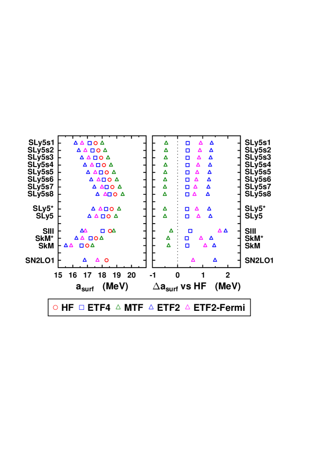
Figure 1: (Color online) Surface energy coefficients obtained within HF (empty circles), MTF (wide triangles) and ETF (empty squares) approaches for the SLy5s series of Skyrme parametrizations (see text). The Figure has been enriched with the standard SIII, SkM, SkM^∗, and SLy5 and SLy5^∗ parametrizations taken as references. The Figure shows also a preliminary HF result for the N2LO SN2LO1 parametrization of Ref.[33].

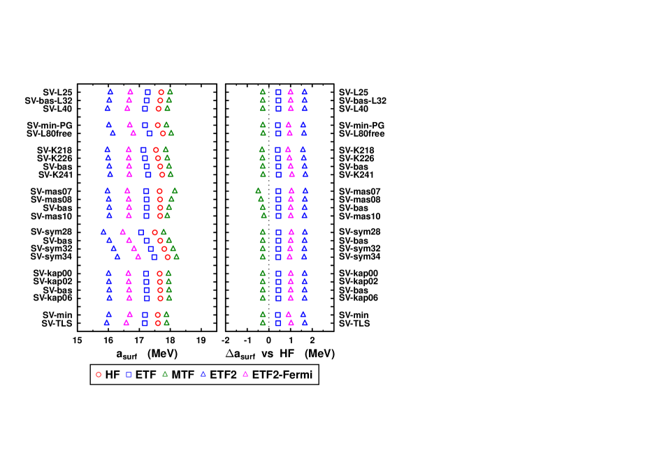
Figure 2: (Color online) Same as Figure 2 for the SV series of NLO Skyrme parametrization (see Refs.[51, 54]).

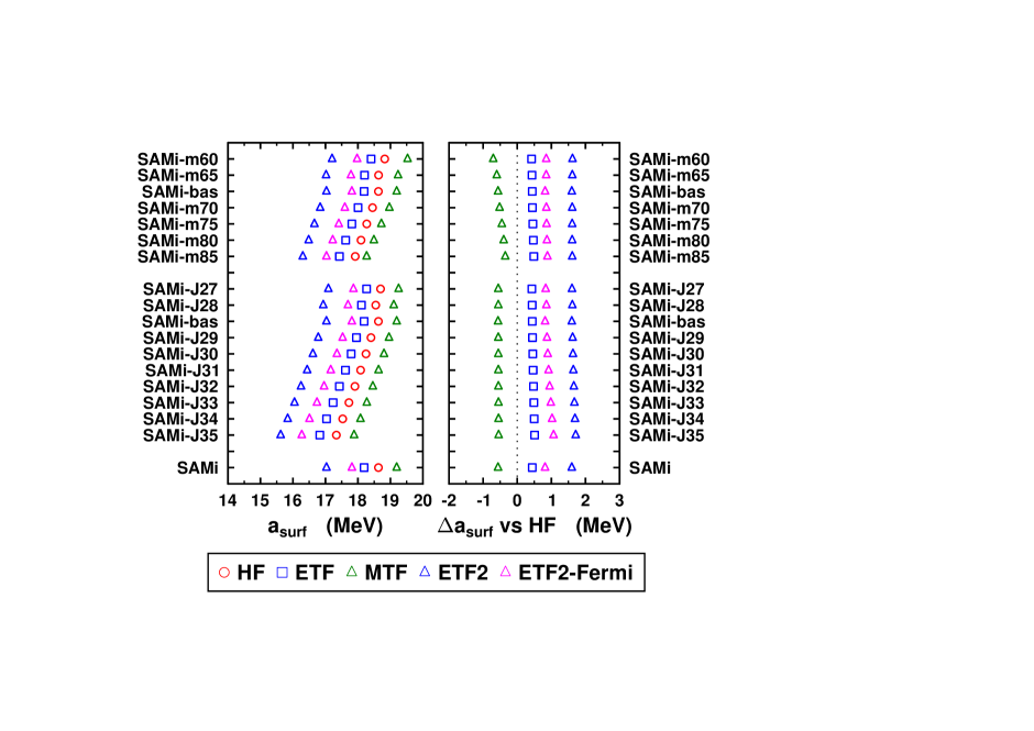
Figure 3: (Color online) Same as Figure 2 for the SAMi series of NLO Skyrme parametrization (see Refs.[52, 55]).

VI Conclusion

The semiclassical calculations are an alternative to Hartree Fock calculations which allow us to derive observables without using wave functions formalism. In this paper, we extended the method developed in Refs.[1, 2] to Skyrme N2LO functionals to get a handly expression of the surface energy. Our results have been obtained within two approximations. The first one is the restriction to the order $\hbar^{2}$ in the Wigner-Kirkwood expansion of the density matrix. This is justified since one of the conclusions of Ref.[1] is the non necessity to expand the density matrix Wigner transform up to $\hbar^{4}$ order to get a good estimate of the surface energy compared to TF and ETF2 approximations. The second approximation lies in neglecting the N2LO terms in the one-body hamiltonian. It comes from the impossibility to derive formally the surface energy because of these terms. It is however justified by the relative size of N2LO terms which are supposed to be small compared to NLO terms (see [33]). With this kind of semiclassical approach, there is a loss of around 1 MeV in the precision of the surface energy with respect to the Hartree Fock results. However, for NLO functionals, the difference between ”exact” Hartree Fock and ETF formula is close to constant: there is only a constant shift between both results which enable us to incorporate the surface energy directly in the fitting procedure. Since the same behavior appears to be true with the N2LO functional of Ref.[33], there is a good hint suggesting the possibility to use the ETF estimations of the surface energy as pseudo-datas for a fitting program of N2LO functionals. One can imagine to construct a similar fitting protocol already used in Ref.[50] to adjust the surface properties In this regards, the results of this paper open opportunities to fit new N2LO parametrizations which shall incorporates new fundamental features by construction.

Appendix A N2LO one body hamiltonian

We give here all the expressions of the various parts of the N2LO one body hamiltonian (see Eq. (5)). We have successively (omitting the $\bm{\mathbf{r}}$ dependence of the densities in the right hand sides for sake of simplicity)

• central fields

  $$U_{q}^{\text{NLO}}(\bm{\mathbf{r}}) = \,2\,\left[\,C_{0}^{\rho}\,-\,C_{1}^{\rho}\,\right]\,\rho_{0}\,+\,4\,C_{1}^{\rho}\,\rho_{q}$$ (49a)

  $$\,+\,2\,\left[\,C_{0}^{\rho^{\gamma}}\,-\,C_{1}^{\rho^{\gamma}}\,\right]\,\rho_{0}^{\gamma}\,\rho_{0}\,+\,4\,C_{1}^{\rho^{\gamma}}\,\rho_{0}^{\gamma}\,\rho_{q}\,+\,{\gamma}\,\left[\,C_{0}^{\rho^{\gamma}}\,+\,C_{1}^{\rho^{\gamma}}\,\right]\,\rho_{0}^{{\gamma}+1}\,-\,4\,{\gamma}\,C_{1}^{\rho^{\gamma}}\,\rho_{0}^{\gamma}\,\rho_{q}\,+\,4\,{\gamma}\,C_{1}^{\rho^{\gamma}}\,\rho_{0}^{{\gamma}-1}\,\rho_{q}^{2}$$

  $$\,+\,2\,\left[\,C^{\Delta\rho}_{0}\,-\,C^{\Delta\rho}_{1}\,\right]\,\Delta\rho_{0}\,+\,4\,C^{\rho}_{1}\,\Delta\rho_{q}\,+\,\left[\,C^{\tau}_{0}\,-\,C^{\tau}_{1}\,\right]\,\tau_{0}\,+\,2\,C^{\tau}_{1}\,\tau_{q}$$

  $$\,+\,\left[\,C^{\nabla J}_{0}\,-\,C^{\nabla J}_{1}\,\right]\,\left(\nabla_{\kappa}\,J_{\kappa,0}\right)\,+\,2\,C^{\nabla J}_{1}\,\left(\nabla_{\kappa}\,J_{\kappa,q}\right)\quad,$$

  $$U_{q}^{\text{N2LO}}(\bm{\mathbf{r}}) = \,2\,\left[\,C_{0}^{(\Delta\rho)^{2}}\,-\,C_{1}^{(\Delta\rho)^{2}}\,\right]\,\Delta\Delta\rho_{0}\,+\,2\,C_{1}^{(\Delta\rho)^{2}}\,\Delta\Delta\rho_{q}$$ (49b)

  $$\,+\,\left[\,C_{0}^{M\rho}\,-\,C_{1}^{M\rho}\,\right]\,Q_{0}\,+\,2\,C_{1}^{M\rho}\,Q_{q}\,-\,2\,\left[\,C_{0}^{M\rho}\,-\,C_{1}^{M\rho}\,\right]\,\nabla_{\mu}\nabla_{\nu}\tau_{0,\mu\nu}^{(s)}\,-\,4\,C_{1}^{M\rho}\,\nabla_{\mu}\nabla_{\nu}\tau_{q,\mu\nu}^{(s)}\quad,$$

  where the density dependent coupling constants $C_{t}^{\rho}\left[\rho_{0}\right]$ have been expanded as already noticed in Eq. (4a).

• effective mass fields

  $$B_{q}^{\text{NLO}}(\bm{\mathbf{r}}) = \,\frac{\hbar^{2}}{2m}\,+\,\left[\,C^{\tau}_{0}\,-\,C^{\tau}_{1}\,\right]\,\rho_{0}\,+\,2\,C^{\tau}_{1}\,\rho_{q}\quad,$$ (50a)

  $$B_{q,\mu\nu}^{\text{N2LO}}(\bm{\mathbf{r}}) = \,2\,\left[\,C_{0}^{M\rho}\,-\,C_{1}^{M\rho}\,\right]\,\tau_{0}\delta_{\mu\nu}\,+\,4\,C_{1}^{M\rho}\,\tau_{q}\delta_{\mu\nu}\,+\,4\,\left[\,C_{0}^{M\rho}\,-\,C_{1}^{M\rho}\,\right]\,\tau^{(s)}_{0,\mu\nu}\,+\,8\,C_{1}^{M\rho}\,\tau^{(s)}_{q,\mu\nu}$$ (50b)

  $$\,-\,2\,\left[\,C_{0}^{M\rho}\,-\,C_{1}^{M\rho}\right]\,\nabla_{\mu}\nabla_{\nu}\rho_{0}\,-\,4\,C_{1}^{M\rho}\,\nabla_{\mu}\nabla_{\nu}\rho_{q}\quad,$$

  $$D_{q}^{\text{N2LO}}(\bm{\mathbf{r}}) = \,\left[\,C_{0}^{M\rho}\,-\,C_{1}^{M\rho}\,\right]\,\rho_{0}\,+\,2\,C_{1}^{M\rho}\,\rho_{q}\quad.$$ (50c)

• spin-orbit fields

  $$\bm{\mathbf{W}}_{q}^{\text{NLO}}(\bm{\mathbf{r}}) = \,-\,\left[\,C^{\nabla J}_{0}\,-\,C^{\nabla J}_{1}\,\right]\,\bm{\mathbf{\nabla}}\rho_{0}\,-\,2\,C^{\nabla J}_{1}\,\bm{\mathbf{\nabla}}\rho_{q}\,-\,\left[\,C^{T}_{0}\,-\,C^{T}_{1}\,\right]\,\bm{\mathbf{J}}_{0}\,-\,2\,C^{T}_{1}\,\bm{\mathbf{J}}_{q}\quad,$$ (51a)

  $$\bm{\mathbf{W}}_{q}^{\text{N2LO}}(\bm{\mathbf{r}}) = \,2\,\left[\,C_{0}^{MT}\,-\,C_{1}^{MT}\,\right]\,\bm{\mathbf{C}}_{0}\,+\,4\,C_{1}^{MT}\,\bm{\mathbf{C}}_{q}\quad,$$ (51b)

  $$\bm{\mathbf{V}}_{q}^{\text{N2LO}}(\bm{\mathbf{r}}) = \,2\,\left[\,C_{0}^{MT}\,-\,C_{1}^{MT}\,\right]\,\bm{\mathbf{J}}_{0}\,+\,4\,C_{1}^{MT}\,\bm{\mathbf{J}}_{q}\quad.$$ (51c)

Appendix B Explicit expressions of $\hat{\cal G}_{i}$ and $\hat{\alpha}_{i}$ functions

If we use the explicit expressions of $H_{q,cl}$ and ${\bf H_{q,so}}$ with ${\bf x}=({\bf r},{\bf p})$, we obtain:

$$\hat{\cal G}_{q,0}({\bf x},\hbar) =\hat{\mathbb{1}}_{\sigma}$$

$$\hat{\cal G}_{q,1}({\bf x},\hbar) =\hbar\,({\bf g}_{q}\times\bm{\mathbf{p}})\cdot\hat{\bm{\mathbf{\sigma}}}$$

$$\hat{\cal G}_{q,2}({\bf x},\hbar) =\frac{\hbar^{2}}{8m^{2}}\big{[}8m^{2}{\bf g}_{q}^{2}\bm{\mathbf{p}}^{2}-8m^{2}({\bf g}_{q}\cdot\bm{\mathbf{p}})^{2}+2(\bm{\mathbf{p}}\cdot\bm{\mathbf{\nabla}}f_{q})^{2}-f_{q}\bm{\mathbf{p}}^{2}\Delta f_{q}-2mf_{q}\Delta V_{q}\big{]}\hat{\mathbb{1}}_{\sigma}+{\cal O}(\hbar^{3})$$

$$\hat{\cal G}_{q,3}({\bf x},\hbar) =\frac{\hbar^{2}}{16m^{3}}\big{[}4f_{q}\bm{\mathbf{p}}^{2}(\bm{\mathbf{p}}\cdot\bm{\mathbf{\nabla}}f_{q})^{2}+8mf_{q}(\bm{\mathbf{p}}\cdot\bm{\mathbf{\nabla}}f_{q})(\bm{\mathbf{p}}\cdot\bm{\mathbf{\nabla}}V_{q})-2f^{2}_{q}\bm{\mathbf{p}}^{2}(\bm{\mathbf{p}}\cdot\bm{\mathbf{\nabla}})^{2}f_{q}-4mf_{q}^{2}(\bm{\mathbf{p}}\cdot\bm{\mathbf{\nabla}})^{2}V_{q}-f_{q}\bm{\mathbf{p}}^{4}(\bm{\mathbf{\nabla}}f_{q})^{2}$$

$$\phantom{=}\ -4mf_{q}\bm{\mathbf{p}}^{2}(\bm{\mathbf{\nabla}}f_{q})\cdot(\bm{\mathbf{\nabla}}V_{q})-4m^{2}f_{q}(\bm{\mathbf{\nabla}}V_{q})^{2}\big{]}\hat{\mathbb{1}}_{\sigma}+{\cal O}(\hbar^{3})$$ (52)

We thus get

$$\hat{\alpha}_{q,3}= \frac{p_{F}^{3}}{3}\hat{\mathbb{1}}_{\sigma}+\hbar^{2}\bigg{[}p_{F,q}\bigg{(}\frac{m^{2}{\bf g_{q}}^{2}}{f_{q}^{2}}+\frac{7(\bm{\mathbf{\nabla}}f_{q})^{2}}{96f_{q}^{2}}-\frac{\Delta f_{q}}{12f_{q}}\bigg{)}+\frac{m}{p_{F,q}}\bigg{(}\frac{(\bm{\mathbf{\nabla}}f_{q})\cdot(\bm{\mathbf{\nabla}}V_{q})}{24f_{q}^{2}}-\frac{\Delta V_{q}}{12f_{q}}\bigg{)}+\frac{m^{2}}{p_{F,q}^{3}}\bigg{(}-\frac{(\bm{\mathbf{\nabla}}V_{q})^{2}}{24f_{q}^{2}}\bigg{)}\bigg{]}\hat{\mathbb{1}}_{\sigma}$$

$$+\mathcal{\cal O}(\hbar^{3})$$ (53)

$$\hat{\alpha}_{q,4,\mu}= -\hbar\frac{m\ p_{F,q}^{3}}{3f_{q}}(\hat{\bm{\mathbf{\sigma}}}\times{\bf g_{q}})_{\mu}+\mathcal{\cal O}(\hbar^{3})$$ (54)

$$\hat{\alpha}_{q,5,\mu\nu}= \frac{p_{F,q}^{5}\delta_{\mu\nu}}{15}\hat{\mathbb{1}}_{\sigma}+\hbar^{2}\bigg{[}p_{F,q}^{3}\bigg{(}\frac{2m^{2}{\bf g_{q}}^{2}\delta_{\mu\nu}}{3f_{q}^{2}}-\frac{m^{2}g_{q,\mu}g_{q,\nu}}{3f_{q}^{2}}+\frac{19(\bm{\mathbf{\nabla}}f_{q})^{2}\delta_{\mu\nu}}{288f_{q}^{2}}-\frac{(\nabla_{\mu}f_{q})(\nabla_{\nu}f_{q})}{9f_{q}^{2}}-\frac{(\Delta f_{q})\delta_{\mu\nu}}{18f_{q}}+\frac{7(\nabla_{\mu}\nabla_{\nu}f_{q})}{72f_{q}}\bigg{)}$$

$$+m\ p_{F,q}\bigg{(}\frac{\nabla_{\mu}\nabla_{\nu}V_{q}}{12f_{q}}-\frac{(\Delta V_{q})\delta_{\mu\nu}}{12f_{q}}+\frac{(\bm{\mathbf{\nabla}}f_{q})\cdot(\bm{\mathbf{\nabla}}V_{q})\delta_{\mu\nu}}{8f_{q}^{2}}-\frac{(\nabla_{\mu}f_{q})(\nabla_{\nu}V_{q})}{12f_{q}^{2}}-\frac{(\nabla_{\nu}f_{q})(\nabla_{\mu}V_{q})}{12f_{q}^{2}}\bigg{)}$$

$$+\frac{m^{2}}{p_{F,q}}\bigg{(}\frac{(\bm{\mathbf{\nabla}}V_{q})^{2}\delta_{\mu\nu}}{24f_{q}^{2}}\bigg{)}\bigg{]}\hat{\mathbb{1}}_{\sigma}+\mathcal{\cal O}(\hbar^{3})$$ (55)

$$\hat{\alpha}_{q,5}= \frac{p_{F,q}^{5}}{5}\hat{\mathbb{1}}_{\sigma}+\hbar^{2}\bigg{[}p_{F,q}^{3}\bigg{(}\frac{5m^{2}{\bf g_{q}}^{2}}{3f_{q}^{2}}+\frac{25(\bm{\mathbf{\nabla}}f_{q})^{2}}{288f_{q}^{2}}-\frac{5(\Delta f_{q})}{72f_{q}}\bigg{)}+m\ p_{F,q}\bigg{(}\frac{5(\bm{\mathbf{\nabla}}f_{q})\cdot(\bm{\mathbf{\nabla}}V_{q})}{24f_{q}^{2}}-\frac{\Delta V_{q}}{6f_{q}}\bigg{)}+\frac{m^{2}}{p_{F,q}}\bigg{(}\frac{(\bm{\mathbf{\nabla}}V_{q})^{2}}{8f_{q}^{2}}\bigg{)}\bigg{]}\hat{\mathbb{1}}_{\sigma}$$

$$+\mathcal{\cal O}(\hbar^{3})$$ (56)

$$\hat{\alpha}_{q,6,\mu}= -\hbar\frac{m\ p_{F,q}^{5}}{3f_{q}}(\hat{\bm{\mathbf{\sigma}}}\times{\bf g_{q}})_{\mu}+\mathcal{\cal O}(\hbar^{3})$$ (57)

$$\hat{\alpha}_{q,7}= \frac{p_{F,q}^{7}}{7}\hat{\mathbb{1}}_{\sigma}+\hbar^{2}\bigg{[}p_{F,q}^{5}\bigg{(}\frac{7m^{2}{\bf g_{q}}^{2}}{3f_{q}^{2}}+\frac{7(\bm{\mathbf{\nabla}}f_{q})^{2}}{96f_{q}^{2}}\bigg{)}+m\ p_{F,q}^{3}\bigg{(}\frac{35(\bm{\mathbf{\nabla}}f_{q})\cdot(\bm{\mathbf{\nabla}}V_{q})}{72f_{q}^{2}}-\frac{5(\Delta V_{q})}{36f_{q}}\bigg{)}+m^{2}p_{F,q}\bigg{(}\frac{5(\bm{\mathbf{\nabla}}V_{q})^{2}}{8f_{q}^{2}}\bigg{)}\bigg{]}\hat{\mathbb{1}}_{\sigma}$$

$$+\mathcal{\cal O}(\hbar^{3})$$ (58)

where $p_{F,q}$ is the Fermi momentum. The corresponding Fermi energy is given by $f_{q}\frac{p_{F,q}^{2}}{2m}+V_{q}=E_{F,q}$. Since densities and currents are not space independent, the Fermi momentum and the fields $f_{q}$ and $V_{q}$ depend on the space variables unlike $E_{F,q}$. Thus, we get

$$m\nabla_{\mu}V_{q} =-\frac{p^{2}_{F,q}(\nabla_{\mu}f_{q})}{2}-p_{F,q}f_{q}(\nabla_{\mu}p_{F,q})$$

$$m\nabla_{\mu}\nabla_{\nu}V_{q} =-\frac{p^{2}_{F,q}(\nabla_{\mu}\nabla_{\nu}f_{q})}{2}-p_{F,q}(\nabla_{\mu}f_{q})(\nabla_{\nu}p_{F,q})-p_{F,q}(\nabla_{\nu}f_{q})(\nabla_{\mu}p_{F,q})$$

$$-p_{F,q}f_{q}(\nabla_{\mu}\nabla_{\nu}p_{F,q})-f_{q}(\nabla_{\mu}p_{F,q})(\nabla_{\nu}p_{F,q})$$ (59)

so that :

$$\hat{\alpha}_{q,3}= \frac{p_{F,q}^{3}}{3}\hat{\mathbb{1}}_{\sigma}+\hbar^{2}p_{F,q}\bigg{(}\frac{m^{2}{\bf g_{q}}^{2}}{f_{q}^{2}}+\frac{(\bm{\mathbf{\nabla}}f_{q})^{2}}{24f_{q}^{2}}-\frac{\Delta f_{q}}{24f_{q}}+\frac{(\bm{\mathbf{\nabla}}f_{q})\cdot(\bm{\mathbf{\nabla}}p_{F,q})}{12f_{q}p_{F,q}}+\frac{\Delta p_{F,q}}{12p_{F,q}}+\frac{(\bm{\mathbf{\nabla}}p_{F,q})^{2}}{24p_{F,q}^{2}}\bigg{)}\hat{\mathbb{1}}_{\sigma}+\mathcal{\cal O}(\hbar^{3})$$ (60)

$$\hat{\alpha}_{q,4,\mu}= -\hbar\frac{m\ p_{F,q}^{3}}{3f_{q}}(\hat{\bm{\mathbf{\sigma}}}\times{\bf g})_{\mu}+\mathcal{\cal O}(\hbar^{3})$$ (61)

$$\hat{\alpha}_{q,5,\mu\nu}= \frac{p_{F,q}^{5}\delta_{\mu\nu}}{15}\hat{\mathbb{1}}_{\sigma}+\hbar^{2}p_{F,q}^{3}\bigg{(}\frac{2m^{2}{\bf g_{q}}^{2}\delta_{\mu\nu}}{3f^{2}_{q}}-\frac{m^{2}g_{q,\mu}g_{q,\nu}}{3f^{2}_{q}}+\frac{(\bm{\mathbf{\nabla}}f_{q})^{2}\delta_{\mu\nu}}{72f^{2}_{q}}-\frac{(\nabla_{\mu}f_{q})(\nabla_{\nu}f_{q})}{36f^{2}_{q}}-\frac{(\Delta f_{q})\delta_{\mu\nu}}{72f_{q}}+\frac{\nabla_{\mu}\nabla_{\nu}f_{q}}{18f_{q}}$$

$$-\frac{\nabla_{\mu}\nabla_{\nu}p_{F,q}}{12p_{F,q}}+\frac{(\Delta p_{F,q})\delta_{\mu\nu}}{12p_{F,q}}+\frac{(\bm{\mathbf{\nabla}}f_{q})\cdot(\bm{\mathbf{\nabla}}p_{F,q})\delta_{\mu\nu}}{12f_{q}p_{F,q}}-\frac{(\nabla_{\mu}p_{F,q})(\nabla_{\nu}p_{F,q})}{12p^{2}_{F,q}}+\frac{(\bm{\mathbf{\nabla}}p_{F,q})^{2}\delta_{\mu\nu}}{8p_{F,q}^{2}}\bigg{)}\hat{\mathbb{1}}_{\sigma}+\mathcal{\cal O}(\hbar^{3})$$ (62)

$$\hat{\alpha}_{q,5}= \frac{p^{5}_{F,q}}{5}\hat{\mathbb{1}}_{\sigma}+\hbar^{2}p^{3}_{F,q}\bigg{(}\frac{5m^{2}{\bf g_{q}}^{2}}{3f^{2}_{q}}+\frac{(\bm{\mathbf{\nabla}}f_{q})^{2}}{72f^{2}_{q}}+\frac{\Delta f_{q}}{72f_{q}}+\frac{(\bm{\mathbf{\nabla}}f_{q})\cdot(\bm{\mathbf{\nabla}}p_{F,q})}{4f_{q}p_{F,q}}+\frac{\Delta p_{F,q}}{6p_{F,q}}+\frac{7(\bm{\mathbf{\nabla}}p_{F,q})^{2}}{24p^{2}_{F,q}}\bigg{)}\hat{\mathbb{1}}_{\sigma}+\mathcal{\cal O}(\hbar^{3})$$ (63)

$$\hat{\alpha}_{q,6,\mu}= -\hbar\frac{m\ p^{5}_{F,q}}{3f_{q}}(\hat{\bm{\mathbf{\sigma}}}\times{\bf g_{q}})_{\mu}+\mathcal{\cal O}(\hbar^{3})$$ (64)

$$\hat{\alpha}_{q,7}= \frac{p^{7}_{F,q}}{7}\hat{\mathbb{1}}_{\sigma}+\hbar^{2}p^{5}_{F,q}\bigg{(}\frac{7m^{2}{\bf g_{q}}^{2}}{3f^{2}_{q}}+\frac{5(\Delta f_{q})}{72f_{q}}-\frac{(\bm{\mathbf{\nabla}}f_{q})^{2}}{72f^{2}_{q}}+\frac{5(\bm{\mathbf{\nabla}}f_{q})\cdot(\bm{\mathbf{\nabla}}p_{F,q})}{12f_{q}p_{F,q}}+\frac{5(\Delta p_{F,q})}{36p_{F,q}}+\frac{55(\bm{\mathbf{\nabla}}p_{F,q})^{2}}{72p^{2}_{F,q}}\bigg{)}\hat{\mathbb{1}}_{\sigma}+\mathcal{\cal O}(\hbar^{3})$$ (65)

Appendix C Density dependent term in the $C^{\text{NLO, TF}}$ coefficient

The $C^{\text{NLO, TF}}$ coefficient of the surface energy (see Eq. (42)) is obviously dependent of the exponent $\gamma$ of the density dependence occurring in the Skyrme EDF. In the text, i.e. in Eq. (42), we gave the result for $\gamma=1$. In the general case, the contribution due to the density-dependent term, namely

$$C^{\text{NLO, TF}} \equiv \,-\,C_{0}^{\rho^{\gamma}}\,\rho_{0}^{3}\,\frac{3}{2}\quad,$$ (66)

has to be replaced by

$$C^{\text{NLO, TF}} \equiv \,-\,\,C_{0}^{\rho^{\gamma}}\,\rho_{0}^{\gamma+2}\,C_{\gamma}\quad,$$ (67)

where the $C_{\gamma}$ coefficient can be read in Table 2 for the density dependencies commonly used in the literature.

$\gamma$		$C_{\gamma}$
$1$		$\frac{3}{2}$
$2/3$		$\frac{21}{10}+\frac{\pi}{2\sqrt{3}}-\frac{3\log 3}{2}$
$1/2$		$\frac{8}{3}-\log 4$
$1/3$		$\frac{15}{4}-\frac{\pi}{2\sqrt{3}}-\frac{3\log 3}{2}$
$1/4$		$\frac{24}{5}-\frac{\pi}{2}-\log 8$
$1/5$		$\frac{35}{6}-\frac{5\log 5}{4}-\frac{\sqrt{5}}{4}\log\frac{\sqrt{5}+1}{\sqrt{5}-1}-\frac{\pi}{2}\sqrt{1+\frac{2}{\sqrt{5}}}$
$1/6$		$\frac{48}{7}-\frac{\pi\sqrt{3}}{2}-\frac{3\log 3}{2}-\log 4$

Table 2: Expressions of the $C_{\gamma}$ coefficient (see text) according to the value of the power of the density dependent term in the NLO Skyrme EDF.

References

- Grammaticos and Voros [1979] B. Grammaticos and A. Voros, Semiclassical Approximations for Nuclear Hamiltonians. 1. Spin Independent Potentials, Annals Phys. 123, 359 (1979).
- Grammaticos and Voros [1980] B. Grammaticos and A. Voros, Semiclassical Approximations for Nuclear Hamiltonians. 2. Spin Dependent Potentials, Annals Phys. 129, 153 (1980).
- Myers [1990] W. D. Myers, The surface energy and the compressibility (1990).
- Stocker [1980] W. Stocker, On the surface energy of compressible nuclei, Nucl. Phys. A 342, 293 (1980).
- Bartel et al. [1982] J. Bartel, P. Quentin, M. Brack, C. Guet, and H. B. Hakansson, Towards a better parametrisation of Skyrme-like effective forces: A Critical study of the SkM force, Nucl. Phys. A 386, 79 (1982).
- Ryssens et al. [2019] W. Ryssens, M. Bender, K. Bennaceur, P. H. Heenen, and J. Meyer, Impact of the surface energy coefficient on the deformation properties of atomic nuclei as predicted by Skyrme energy density functionals, Phys. Rev. C 99, 044315 (2019), arXiv:1809.04406 [nucl-th] .
- Stevenson [2020] P. D. Stevenson, Role of the Surface Energy in Heavy-Ion Collisions, EPJ Web Conf. 232, 03005 (2020), arXiv:1911.03559 [nucl-th] .
- Salehi and Ghodsi [2011] M. Salehi and O. N. Ghodsi, The role of surface energy coefficient in heavy ion reactions and improved proximity model, Int. J. Mod. Phys. E 20, 2337 (2011).
- Dutt and Puri [2010] I. Dutt and R. K. Puri, The role of surface energy coefficients and nuclear surface diffuseness in the fusion of heavy-ions, Phys. Rev. C 81, 047601 (2010), arXiv:1004.0495 [nucl-th] .
- Gharaei and Ghodsi [2015] R. Gharaei and O. N. Ghodsi, Role of Surface Energy Coefficients and Temperature in the Fusion Reactions Induced by Weakly Bound Projectiles, Commun. Theor. Phys. 64, 185 (2015).
- Golshanian et al. [2013] M. Golshanian, O. N. Ghodsi, and R. Gharaei, Role of surface Energy Coefficient and Temperature of Compound Nucleus in the -Decay process, Mod. Phys. Lett. A 28, 1350164 (2013).
- Toshniwal and Kumari [2013] A. Toshniwal and R. Kumari, Systematic study of the fusion barriers using different versions of surface energy coefficients, DAE Symp. Nucl. Phys. 58, 420 (2013).
- Goutte et al. [2005] H. Goutte, J. F. Berger, and D. Gogny, Fission: Potential Energy Surfaces and Dynamics, AIP Conf. Proc. 769, 1203 (2005).
- Rajeswari et al. [2017] N. S. Rajeswari, C. Nivetha, and M. Balasubramaniam, Role of surface energy coefficients in cluster decay, DAE Symp. Nucl. Phys. 62, 526 (2017).
- Ravenhall et al. [1972] D. G. Ravenhall, C. D. Bennett, and C. J. Pethick, Nuclear Surface Energy and Neutron-Star Matter, Phys. Rev. Lett. 28, 978 (1972).
- Goriely et al. [2007] S. Goriely, M. Samyn, and J. M. Pearson, Further explorations of Skyrme-Hartree-Fock-Bogoliubov mass formulas. VII. Simultaneous fits to masses and fission barriers, Phys. Rev. C 75, 064312 (2007).
- Nikolov et al. [2011] N. Nikolov, N. Schunck, W. Nazarewicz, M. Bender, and J. Pei, Surface Symmetry Energy of Nuclear Energy Density Functionals, Phys. Rev. C 83, 034305 (2011), arXiv:1012.5829 [nucl-th] .
- Krivine et al. [1980] H. Krivine, J. Treiner, and O. Bohigas, Derivation of a fluid-dynamical lagrangian and electric giant resonances, Nuclear Physics A 336, 155 (1980).
- Brack et al. [1985] M. Brack, C. Guet, and H.-B. Håkansson, Selfconsistent semiclassical description on average nuclear properties - A link between microscopic and macroscopic models, Phys. Rep. 123, 1 (1985).
- Schunck et al. [2014] N. Schunck, D. Duke, H. Carr, and A. Knoll, Description of induced nuclear fission with skyrme energy functionals: Static potential energy surfaces and fission fragment properties, Phys. Rev. C 90, 054305 (2014).
- Côté and Pearson [1978] J. Côté and J. M. Pearson, Hartree-fock calculations of semi-infinite nuclear matter with complete forces (finite-range and spin-orbit term), Nucl. Phys. A 304, 104 (1978).
- Brack and Bhaduri [1997] M. Brack and R. Bhaduri, Semiclassical Physicsl (Addison-Wesley, Reading, USA, 1997) frontiers in Physics.
- Brack et al. [1976] M. Brack, B. K. Jennings, and Y. H. Chu, On the extended Thomas-Fermi approximation to the kinetic energy density, Phys. Lett. B 65, 1 (1976).
- Jennings [1976] B. Jennings, Extended Thomas-Fermi theory for non interacting particles, Ph.D. thesis, Mac Master Universitty, Hamilton, Ontario, Canada (1976).
- Strutinsky [1967] V. Strutinsky, Shell effects in nuclear masses and deformation energies, Nuclear Physics A 95, 420 (1967).
- Strutinsky [1968] V. Strutinsky, “shells” in deformed nuclei, Nuclear Physics A 122, 1 (1968).
- Brack and Pauli [1973] M. Brack and H. Pauli, On strutinsky’s averaging method, Nuclear Physics A 207, 401 (1973).
- Brack and Quentin [1975] M. Brack and P. Quentin, Self-consistent average density matrices and the strutinsky energy theorem, Phys. Lett. B 56, 421 (1975).
- Brack and Quentin [1981] M. Brack and P. Quentin, The strutinsky method and its foundation from the hartree-fock-bogoliubov approximation at finite temperature, Nucl. Phys. A 361, 35 (1981).
- Jodon et al. [2016a] R. Jodon, M. Bender, K. Bennaceur, and J. Meyer, Constraining the surface properties of effective Skyrme interactions, Phys. Rev. C 94, 024335 (2016a), arXiv:1606.01410 [nucl-th] .
- Krivine and Treiner [1979] H. Krivine and J. Treiner, A simple approximation to the nuclear kinetic energy density, Phys. Lett. B 88, 212 (1979).
- Treiner and Krivine [1986] J. Treiner and H. Krivine, Semi-classical nuclear properties from effective interactions, Ann. Phys. (N.-Y.) 170, 406 (1986).
- Becker et al. [2017] P. Becker, D. Davesne, J. Meyer, J. Navarro, and A. Pastore, Solution of hartree-fock-bogoliubov equations and fitting procedure using the n2lo skyrme pseudopotential in spherical symmetry, Phys. Rev. C 96, 044330 (2017).
- Carlsson et al. [2008] B. G. Carlsson, J. Dobaczewski, and M. Kortelainen, Local nuclear energy density functional at next-to-next-to-next-to-leading order, Phys. Rev. C 78, 044326 (2008).
- Carlsson and Dobaczewski [2010] B. G. Carlsson and J. Dobaczewski, Convergence of density-matrix expansions for nuclear interactions, Phys. Rev. Lett. 105, 122501 (2010).
- Raimondi et al. [2011a] F. Raimondi, B. G. Carlsson, and J. Dobaczewski, Effective pseudopotential for energy density functionals with higher-order derivatives, Phys. Rev. C 83, 054311 (2011a).
- Raimondi et al. [2011b] F. Raimondi, B. G. Carlsson, J. Dobaczewski, and J. Toivanen, Continuity equation and local gauge invariance for the n3lo nuclear energy density functionals, Phys. Rev. C 84, 064303 (2011b).
- Ryssens and Bender [2021] W. Ryssens and M. Bender, Skyrme pseudopotentials at next-to-next-to-leading order: Construction of local densities and first symmetry-breaking calculations, Phys. Rev. C 104, 044308 (2021).
- Davesne et al. [2013] D. Davesne, A. Pastore, and J. Navarro, Skyrme effective pseudopotential up to the next-to-next-to-leading order, J. Phys. G 40, 095104 (2013).
- Bender et al. [2003] M. Bender, P.-H. Heener, and P.-G. Reinhard, Self-consistent mean-field models for nuclear structure, Review of Modern Physics 75, 121 (2003).
- Lesinski et al. [2007] T. Lesinski, M. Bender, K. Bennaceur, T. Duguet, and J. Meyer, Tensor part of the skyrme energy density functional: Spherical nuclei, Phys. Rev. C 76, 014312 (2007).
- Sadoudi [2011] J. Sadoudi, Constraints on the nuclear energy density functional and new possible analytical forms, Ph.D. thesis, Université Paris-Sud XI (2011).
- Sadoudi et al. [2013] J. Sadoudi, T. Duguet, J. Meyer, and M. Bender, Skyrme functional from a three-body pseudopotential of second order in gradients: Formalism for central terms, Phys. Rev. C 88, 064326 (2013).
- Weyl [1927] H. Weyl, Quantenmechanik und gruppentheorie, Z. Physik 46, 1 (1927).
- Groenewold [1946] H. Groenewold, On the principles of elementary quantum mechanics, Physica 12, 405 (1946).
- Swiatecki [1951] W. Swiatecki, The nuclear surface energy, Proc. Phys. Soc. A 64, 226 (1951).
- Myers and Swiatecki [1969] W. D. Myers and W. J. Swiatecki, Average nuclear properties, Ann. Phys. (N.-Y.) 55, 395 (1969).
- Myers and Swiatecki [1974] W. Myers and W. Swiatecki, The nuclear droplet model for arbitrary shapes, Annals of Physics 84, 186 (1974).
- Bartel et al. [2008] J. Bartel, K. Bencheikh, and J. Meyer, Extended Thomas-Fermi density functionals in the presence of a tensor interaction in spherical symmetry, Phys. Rev. C 77, 024311 (2008).
- Jodon et al. [2016b] R. Jodon, M. Bender, K. Bennaceur, and J. Meyer, Constraining the surface properties of effective skyrme interactions, Phys. Rev. C 94, 024335 (2016b).
- Klüpfel et al. [2009] P. Klüpfel, P.-G. Reinhard, T. J. Bürvenich, and J. A. Maruhn, Variations on a theme by skyrme: A systematic study of adjustments of model parameters, Phys. Rev. C 79, 034310 (2009).
- Roca-Maza et al. [2012] X. Roca-Maza, G. Colò, and H. Sagawa, New skyrme interaction with improved spin-isospin properties, Phys. Rev. C 86, 031306 (2012).
- Bender [2022] M. Bender (2022), private communication.
- Reinhard [2016] P.-G. Reinhard (2016), private communication.
- Colò [2016] G. Colò (2016), private communication.