MUG: Multi-human Graph Network for 3D Mesh Reconstruction from 2D Pose

Abstract

Reconstructing multi-human body mesh from a single monocular image is an important but challenging computer vision problem. In addition to the individual body mesh models, we need to estimate relative 3D positions among subjects to generate a coherent representation. In this work, through a single graph neural network, named MUG (Multi-hUman Graph network), we construct coherent multi-human meshes using only multi-human 2D pose as input. Compared with existing methods, which adopt a detection-style pipeline (i.e., extracting image features and then locating human instances and recovering body meshes from that) and suffer from the significant domain gap between lab-collected training datasets and in-the-wild testing datasets, our method benefits from the 2D pose which has a relatively consistent geometric property across datasets. Our method works like the following: First, to model the multi-human environment, it processes multi-human 2D poses and builds a novel heterogeneous graph, where nodes across people and within one person are connected to capture inter-human interactions and draw the body geometry (i.e., skeleton and mesh structure). Second, it employs a dual-branch graph neural network structure – one for predicting inter-human depth relation and the other one for predicting root-joint-relative mesh coordinates. Finally, the entire multi-human 3D meshes are constructed by combining the output from both branches. Extensive experiments demonstrate that MUG outperforms previous multi-human mesh estimation methods on standard 3D human benchmarks – Panoptic, MuPoTS-3D and 3DPW.

1 Introduction

Deep learning methods leveraging large-scale datasets have shown tremendous progress on tasks in 3D human mesh recovery, which is often an important initial step in computer vision and robotics applications on human behaviors, such as activity recognition [16] and bodily expressed emotion understanding [44]. For single-human mesh [15, 20, 19, 4, 31] estimation, recent works achieve admirable results. Naturally, it is desirable to extend the success to multi-human scenarios to provide a holistic understanding of a scene.

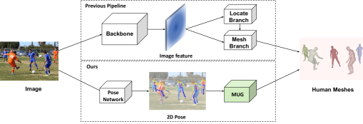
Figure 1: Previous multi-human mesh networks commonly adopt a detection-style pipeline using images as input. In our pipeline, the proposed Multi-hUman Graph network (MUG) takes the 2D pose as input. The 2D pose can be obtained by 2D human pose estimation networks.

Multi-human mesh estimation requires generating body mesh models and providing comprehensive 3D positions for each instance. Most recent methods [13, 56, 40] adopt a detection-style pipeline with whole images as input. As illustrated in Figure 1, they first feed the images into a backbone to extract features. Then one branch locates human instances. The other branch (or branches) will generate body meshes on top of the image feature and instances’ locations. Particularly, [13] leverages the region proposal network (RPN) [36] to propose human body boxes and [56, 40] locate body center points in their locate branches.

However, this pipeline, using images as input, suffers from the domain gap between in-the-wild and lab-collected datasets, which is a widely known problem in 3D-related works [57, 45, 4, 7, 26, 49]. The primary contradiction is that lab-collected datasets [12, 38] are crucial for providing accurate 3D labels in training; While, these images have very different appearance from the in-the-wild testing images. For example, backgrounds and lighting conditions of the images collected in the monotonous laboratory environment are distinct from the images captured from in-the-wild environment. In addition, the domain gap can be more prominent in multi-human mesh estimation. Single-human mesh networks commonly take cropped-and-centered human images as input [19, 20, 31]. Human bodies tend to take up most of the image area and they share more similarities across lab-collected and in-the-wild datasets, whereas there are dramatic differences between the surrounding backgrounds of humans in these two kinds of datasets. In contrast, the multi-human mesh networks take whole images as input [56, 13, 40], where the backgrounds occupy much more areas. That means taking whole images as input may lead to a more significant domain gap, thus preventing multi-human mesh methods from fully utilizing the training data.

To tackle the aforementioned domain gap issue, we hope to build up a new pipeline with the 2D pose as input. Compared with the image features, the 2D pose has relatively consistent geometric properties across different datasets. No matter how environmental characteristics (e.g., lighting and weather) change, the 2D pose remains the body joint coordinates in the images. Also, accurate 2D poses can be obtained through cutting-edge keypoint-detection networks[39, 3, 9] trained on large-scale in-the-wild datasets.

To reconstruct multi-human meshes from the 2D pose, we need to design a network to accomplish the following two goals (1) accurately predict body meshes from the 2D pose, and (2) estimate comprehensive relative 3D body positions from the 2D pose. Regarding the first goal, each body mesh vertex needs to get the coordinate information from surrounding joints and mesh vertices within the human. Therefore, we need to take advantage of the intra-human skeleton and mesh topology. For the second goal, capturing the inter-human dependencies is crucial to obtain the correct relative body positions. In short, we need to model intra- and inter-human relations simultaneously.

In this work, we propose a simple yet effective heterogeneous graph convolutional network MUG (Multi-hUman Graph network). First, we construct a novel heterogeneous graph to represent the holistic multi-human environment. Body joints and mesh vertices are represented as two different types of nodes. Within one human, we connect joint and mesh nodes to form intra-human edges according to the body skeleton structure and mesh topology. To represent inter-human relations, we pick and then connect appropriate joint nodes across humans as edges. Through different kinds of edges, the coordinate information can be transmitted among nodes within a human or across humans. Next, we design a dual branch graph convolutional network structure to simultaneously output root-camera depth and root-relative body mesh coordinates. After feeding the heterogeneous graph and 2D pose input into the neural network, we can construct multi-human meshes by combining the output of the two branches. The entire framework is illustrated in Figure 2.

Extensive experiments show that our method significantly outperforms the previous SOTA [13, 56, 40] on multi-person 3D human datasets–Panoptic [14], MuPoTS-3D [28] and 3DPW [25], where MuPoTS-3D and 3DPW are both in-the-wild datasets. Then we conduct ablation studies to help analyze the effectiveness of the graph construction and the influence of different 2D pose input. We also provide qualitative results.

Our contributions are summarized as follows.

• We design a new pipeline for multi-human reconstruction. With the 2D pose as input, we use one single graph network to output multi-human meshes and 3D locations simultaneously. The consistent geometric property of the 2D pose makes our method more robust to the domain gap.

• We propose a novel graph neural network, named MUG, that leverages the heterogeneous graph, including joint nodes, vertex nodes, and different types of edges, to represent the intra- and inter-human relations.

• Our method significantly outperforms previous approaches on standard multi-person 3D human datasets.

2 Related Work

2.1 Single-human mesh estimation

Single-human mesh estimation aims at reconstructing body mesh in the cropped human image. The body mesh can be represented by the 3D vertex coordinates or the human body models (such as SMPL [24]). According to the method’s output is body mesh model parameters or 3D vertex coordinates, human mesh estimation methods can be divided into two types: model-based and model-free.

Bogo et al. pioneered a model-based method and demonstrated how to fit SMPL parameters by minimizing the error between predicting and input pose [2]. Then the following works mainly adopt an end-to-end neural network to train images and regress SMPL parameters. HMR [15] utilized adversarial loss for its regression network. Pavlakos et al. [34] exploited 2D joint heatmaps and silhouettes as a cue. SPIN [19] introduced optimization methods into the regression network.

Despite the success of these model-based approaches, recent works argue that SMPL parameters, which are in the form of 3D rotation, might not be accessible to learn [20]. As such, more and more recent researches focus on model-free methods. GraphCMR [20] used ResNet to extract global features and GNN to regress 3D vertex coordinates. Inspired by the heatmap representation in 2D pose estimation, Moon et al. [31] developed a new representation, called lixel, to help regress 3D coordinates. Lin et al. [22] built up a transformer network. Choi et al. [4] took the 2D pose as input and exploited 3D pose as intermediate features, then used GNN to estimate body mesh coordinates in a coarse-to-fine manner [52]. Our work also uses 2D pose as input and adopts GNN. However, the single-human problem does not need to estimate the human depth and analyze the human iteration. [4] only outputs root-relative coordinates. When reprojecting body meshes to the original image, [4] cannot distinguish human body orders.

2.2 Multi-human mesh estimation

Multi-human mesh estimation is a relatively new field [53, 54, 13, 56, 40]. Zanfir et al. [53] published a pioneering work in 2018 in which they implemented a top-down approach. First, a multi-task single-human network was used to estimate 2D pose, 3D mesh, and other scene constraints. Then these outputs were jointly optimized to generate the final prediction. In another work in 2018, Zanfir et al. [54] proposed a bottom-up method that first performed 3D pose estimation then used an unsupervised auto-encoder to estimate SMPL parameters. Recent works adopt detection-style pipelines to solve this task and achieve stunning performance. Jiang et al. [13] follows the two-stage detection framework Faster RCNN [36] to use RPN to propose human body boxes. Then it uses SMPL-head to regress SMPL parameters according to proposed boxes. Zhang et al. [56] and ROMP [40] adopt an one-stage solution – using one head to locate the center point of the human, and the other head outputs SMPL parameters according to the center point. As aforementioned, these methods suffer from the domain shift problem.

2.3 Graph neural networks

Graph neural networks (GNNs) learn node embeddings that preserve the graph structure and the original node features [17]. Recently, GNNs have achieved SOTA performance on various computer vision tasks [21, 4, 51, 11]. According to the type of graphs, GNNs can be divided into two categories: homogeneous GNNs [17, 42, 8] and heterogeneous GNNs [37, 48]. The homogeneous GNNs assume all nodes and edges in the graph are of the same type, where most existing work focus on modeling such relations via different approaches, such as graph convolution [17], attention network [42], recurrent neural networks [8], etc. On the other hand, heterogeneous GNNs are proposed for graphs that contain different types of nodes and edges. The diversity of node types and edge types require GNNs to capture the characteristics of each node and edge type. For example, [37] proposes R-GCN where every type of node and edge is modeled by an individual graph convolutional network [17].

3 Method

In this section, we describe our technical approach. The entire framework is illustrated in Figure 2. We describe our proposed heterogeneous multi-human graph in Subsection 3.1. Then we demonstrate the node feature construction in Subsection 3.2. The neural network structure is illustrated in Subsection 3.3. In Subsection 3.4, we analyze the root-camera depth computing. Finally, Subsection 3.5 introduces how to reconstruct multiple humans with network outputs.

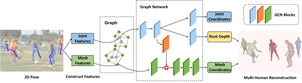
Figure 2: Illustration of the framework. 2D multi-human pose is the input. To explicitly model the inter- and intra-human relation, we build a heterogeneous graph containing joint nodes (blue circles) and mesh nodes (green circles). On top of the graph, we construct node features using 2D pose. The graph network adopts a dual-branch structure. Joint nodes with joint features go through the upper branch (blue blocks), meanwhile mesh nodes with mesh features go through the lower branch (green blocks). One GCN block (orange block) connects these two branches. Finally, the upper branch outputs root-camera depth and the lower branch outputs root-relative mesh coordinates. By combining the outcomes, we can recover the full multi-human meshes. The upper branch also outputs joint coordinates, which plays a supporting role in learning.

3.1 Graph construction

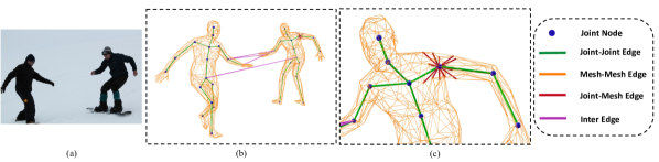
Figure 3: Structure of the graph. The graph consists of two kinds of nodes, joint nodes $\mathcal{V}^{\text{Joint}}$ (blue circles) and mesh nodes $\mathcal{V}^{\text{Mesh}}$. Each human corresponds to one subgraph of the whole graph. Within one human, joint nodes are connected to get edge $\mathcal{E}^{{\text{Joint - Joint}}}$ (green lines) according to body skeleton structure; following body mesh topology, mesh nodes are connected to get edge $\mathcal{E}^{{\text{Mesh - Mesh}}}$ (orange lines); each mesh node connects to its two nearest joint nodes, generating edge $\mathcal{E}^{{\text{Joint - Mesh}}}$ (red lines). To represent inter-human relation, we connect joint nodes across humans to get edge $\mathcal{E}^{\text{Inter}}$ (purple lines). (b-c) shows the graph structure for image (a). For better display, we do not draw mesh nodes and only draw part of edge $\mathcal{E}^{{\text{Joint - Mesh}}}$.

This subsection introduces how to construct the graph of MUG, Figure 3 illustrates the graph structure. Assuming there are $K$ humans in total, we use $\mathcal{G}^{*}$ to denote the entire multi-human graph and $\mathcal{G}_{1},\cdots,\mathcal{G}_{K}$ to denote the subgraph of each human. Each subgraph contains two types of nodes, one is joint node $\mathcal{V}^{\text{Joint}}_{i}$, the other is mesh node $\mathcal{V}^{\text{Mesh}}_{i}$. Joint nodes represent human body keypoints like hips and shoulders (totally $J$ joint nodes within a human), which have 2D coordinate ground truth in training datasets and can be accurately predicted by 2D pose detection networks, such as [9, 39]. Mesh nodes represent the vertices in the body mesh (totally $V$ mesh nodes within a human), our target is to obtain their absolute 3D coordinates.

Let us dive into each subgraph. To represent the body geometric topology, we connect joint nodes according to the body skeleton structure, and we link mesh nodes based on the body mesh topology. Furthermore, we add edges between these two kinds of nodes according to their distance pre-defined by the SMPL body mesh template [24]. Each mesh node connects to its two nearest joint nodes. These edges are directional – only from joint nodes to mesh nodes. The reason is that the input of MUG only has 2D coordinates of joints. Therefore, coordinates information should be transmitted strictly from joint nodes to mesh nodes. Formally, we have each subgraph $\mathcal{G}_{i}=(\mathcal{V}_{i},\mathcal{E}_{i},\mathbf{X}_{i}),i\in\{1,...,K\}$, where node set $\mathcal{V}_{i}=\mathcal{V}^{\text{Joint}}_{i}\cup\mathcal{V}^{\text{Mesh}}_{i}$; edge set $\mathcal{E}_{i}=\mathcal{E}^{\text{Joint - Joint}}_{i}\cup\mathcal{E}^{\text{Mesh - Mesh}}_{i}\cup\mathcal{E}^{\text{Joint - Mesh}}_{i}$; and node features $\mathbf{X}_{i}=\mathbf{X}^{\text{Joint}}_{i}\cup\mathbf{X}^{\text{Mesh}}_{i}$. The node features construction is introduced in Subsection 3.2.

To model the spatial correlation across humans, we further integrate all human subgraphs into a multi-layer graph $\mathcal{G}^{*}=(\mathcal{V}^{*},\mathcal{E}^{*},\mathbf{X}^{*})$. Each layer contains a human subgraph $\mathcal{G}_{i}$, we have $\mathcal{V}^{*}=\{\mathcal{V}_{i}\}_{i=1}^{K},\mathbf{X}^{*}=\{\mathbf{X}_{i}\}_{i=1}^{K}$. We construct edges $\mathcal{E}^{\text{Inter}}$ across different subgraphs to represent the inter-human relation. There are two types of $\mathcal{E}^{\text{Inter}}$: (1) We set a length threshold $\epsilon$, any two joint nodes from different humans will be connected to form an edge if these two joints’ 2D distance in the image is less than $\epsilon$. By selecting appropriate $\epsilon$, pairs of joints in small 2D distances will be connected. The idea is inspired by the first law of geography [41] that points close in space share similar features. A small 3D distance always leads to a small 2D distance. Joints pairs in small 2D distances are relatively more likely to have interaction (e.g. overlap), thus need more accurate prediction. We connect these joints pairs as edges, inducing the GNN to produce better predictions on these joints and around mesh nodes. (2) Any two humans’ root-joint nodes must be connected. The root-joint is usually used to determine the depth of a human from the camera. Relative depth information for each human can be passed through root-to-root edges. More analysis of $\mathcal{E}^{\text{Inter}}$ can be found in the ablation study (Subsection 4.4).

In summary, we have intra-human edges in each human subgraph (including $\mathcal{E}^{{\text{Joint - Joint}}}$, $\mathcal{E}^{{\text{Joint - Mesh}}}$, $\mathcal{E}^{{\text{Mesh - Mesh}}}$) and $\mathcal{E}^{\text{Inter}}$ among the subgraphs to connect individuals. The set of all these edges can be described as $\mathcal{E}^{*}=\mathcal{E}^{\text{Inter}}\cup\{\mathcal{E}_{i}\}_{i=1}^{K}$.

3.2 The node feature construction

We define the node features as $\mathbf{X}^{*}=\{\mathbf{X}_{i}\}_{i=1}^{K}$. The $i^{th}$ human’s feature $\mathbf{X}_{i}$ includes $\mathbf{X}_{i}^{\text{Joint}}\in\mathbb{R}^{J\times d}$ for joint nodes and $\mathbf{X}_{i}^{\text{Mesh}}\in\mathbb{R}^{V\times d}$ for mesh nodes, where $d$ is the feature dimension.

For joint nodes, we denote the feature for the $j^{th}$ joint of the $i^{th}$ human as $\mathbf{X}_{ij}^{\text{Joint}}$. The main information that can be used to construct features is the 2D pose input $P_{i}^{\text{2D}}\in\mathbb{R}^{J\times 2}$. Following previous work [43, 4], we first apply standard normalization to $P_{i}^{\text{2D}}$. Specifically, we subtract the mean of $P_{i}^{\text{2D}}$ and divide by the standard deviation in order to obtain $\overline{P}_{i}^{\text{2D}}$. Then $\overline{P}_{ij}^{\text{2D}}$ is assigned to the $j^{th}$ joint. The normalization [43] allows for easier convergence of the GCN, but it turns each human’s 2D pose into relative coordinates regardless of this human’s body size and position. To analyze relative 3D human positions, we need to compare the absolute joint coordinates across humans in the images. Thus the joint coordinates over the entire image range are necessary to pass to joint nodes. In the meantime, to facilitate training, we need to convert different images into a uniform size. We resize the raw image’s long edge as $1000$ pixels and then center it in the $1000\times 1000$ pixels square. $P_{i}^{\text{2D}}$ will be accordingly transformed into $\widetilde{P}_{i}^{\text{2D}}$. Then $\widetilde{P}_{ij}^{\text{2D}}$ is assigned to the $j^{th}$ joint. To fully utilize $\widetilde{P}_{i}^{\text{2D}}$, we also pass whole $\widetilde{P}_{i}^{\text{2D}}$ to $\mathbf{X}_{ij}^{\text{Joint}}$.

In addition, we leverage 11 SMPL body mesh models, containing the SMPL template model as well as 10 randomly selected from Human3.6M dataset. Mesh vertices coordinates can be computed by these models. For simplicity, we just denote mesh coordinates from one model as $T\in\mathbb{R}^{V\times 3}$. We can compute the 3D coordinates of joints by multiplying $T$ with the joint regression matrix $\mathcal{J}\in\mathbb{R}^{J\times V}$, where $\mathcal{J}$ is defined in SMPL body mesh model [24]. Then we pass $(\mathcal{J}T)_{j}$ to $\mathbf{X}_{ij}^{\text{Joint}}$. Although these body mesh coordinates are fixed, the graph neural network can learn some rigid geometry information by remembering these examples. Finally, the joint feature can be obtained by concatenating above features,

$$~{}\mathbf{X}_{ij}^{\text{Joint}}=(\widetilde{P}_{ij}^{\text{2D}},\widetilde{P}_{i}^{\text{2D}},\overline{P}_{ij}^{\text{2D}},(\mathcal{J}T)_{j})\;.$$ (1)

For mesh nodes, we denote the feature for the $v^{th}$ mesh vertex in $i^{th}$ human as $\mathbf{X}_{iv}^{\text{Mesh}}$. Different from joint nodes, we can not know the $2D$ position information of each mesh vertex by the 2D pose input. We directly use $\widetilde{P}_{ij^{*}}^{\text{2D}}$ and $\overline{P}_{ij^{*}}^{\text{2D}}$ to initialize the mesh features, where $j^{*}$ represents the nearest joint with the $v^{th}$ mesh node in the SMPL body mesh template. Following a similar process with joint nodes, we also feed $\widetilde{P}_{i}^{\text{2D}}$ and $T_{v}$ (the $v^{th}$ vertex in $T$) to $\mathbf{X}_{iv}^{\text{Mesh}}$. Concatenate these features we have,

$$\mathbf{X}_{iv}^{\text{Mesh}}=(\widetilde{P}_{ij^{*}}^{\text{2D}},\widetilde{P}_{i}^{\text{2D}},\overline{P}_{ij^{*}}^{2D},T_{v})\;.$$ (2)

3.3 Network structure

Then we introduce the model structure, which is illustrated in Figure 2. Considering the two kinds of nodes, we design a dual-branch graph network. Joint nodes with joint features go through one branch, meanwhile mesh nodes with mesh features go through the other. The two branches are connected by a GCN block, namely the connection block. For the branch of joint nodes, they first go through two GCN blocks. Then the output has three destinations. One is passed into the mesh branch via the connection block. Another will step into one GCN block and finally reduce its feature dimension into 1. We pick the value of the root-joint node as the depth measure for its human instance. The last one will reduce the dimension into 3 to output 3D joint coordinates through one GCN block. Although these 3D joint coordinates are not used in 3D mesh reconstruction, they can guide the branch to learn depth representation. The other branch consists of four GCN blocks. After passing one GCN block, the mesh nodes will add their features with the output of the connection block. Then, going through three more GCN blocks and reducing their feature dimension into 3, mesh nodes finally output root-related body mesh coordinates. The GCN blocks are the GCN residual block which is inspired by ResNet Basic blocks [10], or just the cascade of three graph convolutional layers. The amount of parameters of the entire network is not large, only 2.3M. The detailed structure and configuration are discussed in the supplementary.

3.4 Estimating depth

For this monocular setting, it is not meaningful to predict an accurate root-camera depth. Here we aim at providing a comprehensive depth estimation to reflect relative 3D position across humans. Skeletons of different humans usually have similar lengths. Through the pine-hole camera model [6], the ratio between the root-camera depth and focal length largely decides the size of the skeletons in the image. Conversely, we attempt to use 2D human pose to infer that ratio. For this, we construct the depth measure as $\widetilde{D}=D/f$, where $D$ is the depth and $f$ is the camera focal length. As mentioned in Subsection 3.2 we resize the raw image to make its long edge width as 1000 pixels, this is equivalent to adjusting the focal length while holding the depth. For the training convenience, we also add a constant coefficient $\alpha$ to make the the measure in the range of [0,1]. Finally, we get the depth measure,

$$\widetilde{D}=\frac{DS}{1000\alpha f}\;,$$ (3)

where $S$ is the long edge width of the raw image and we set $\alpha$ as 200 in practice. In the training process, we utilize the $L1$ loss to supervise $\widetilde{D}$ and adopt a relative depth loss to get more accurate human relative depth,

$$L_{\text{D}}=\lVert\widetilde{D}-\widetilde{D}^{*}\rVert_{1}\;,L_{\text{rD}}=\frac{1}{N}\sum_{m,n}\lVert(\widetilde{D}_{m}-\widetilde{D}_{n})-(\widetilde{D}^{*}_{m}-\widetilde{D}^{*}_{n})\rVert_{1}\;,$$ (4)

where $*$ represents the ground truth and $m,n$ represent different human instances. In training, for the dataset containing root-camera depth and focal length, we can directly compute ground truth $\widetilde{D}$. If the dataset doesn’t provide these labels, we assume $f$ as $1500$. Then we use SMPLify [33] to generate pseudo root-camera depth, such that pseudo $\widetilde{D}$ can be obtained. The assumption of $f$ is sufficient to give the comprehensive depth. Because $f$ is the same for all humans within one image, relative 3D body positions are consistent regardless of the change of $f$. In inference, we can recover the $D$ with $f$, $S$ and predicted $\widetilde{D}$.

3.5 Reconstruct multiple humans

Besides the depth, the graph network also outputs root-relative mesh vertex coordinates $M\in\mathbb{R}^{V\times 3}$ and 3D joint coordinates $P^{\text{3D}}\in\mathbb{R}^{J\times 3}$ for each human, where $M$ is what our need to recover the body mesh and $P^{\text{3D}}$ play a supporting role in training. Also, we can get the 3D joint coordinates from $M$ by multiply the joint regression matrix $\mathcal{J}$. In the training process, we use the $L1$ loss function to supervise $M$, $P^{3D}$ and $\mathcal{J}M$,

$$\begin{split}L_{\text{M}}=||M-M^{*}||_{1}\;,L_{\text{J}}=||P^{\text{3D}}-{P^{\text{3D}}}^{*}||_{1}\;,L_{\text{JM}}=||\mathcal{J}M-{P^{\text{3D}}}^{*}||_{1}\;,\end{split}$$ (5)

where $*$ represents the ground truth. If the dataset doesn’t provide 3D labels for joints or mesh coordinates, we use SMPLify [33] to generate pseudo 3D coordinates ground truth.

Following [47], we also use the mesh normal vector loss $L_{\text{N}}$ and mesh edge vector loss $L_{\text{N}}$ to make the mesh result more smooth. These losses and above losses for depth are then summed together to get the total loss,

$$L=L_{\text{M}}+\lambda_{1}L_{\text{J}}+\lambda_{2}L_{\text{JM}}+\lambda_{3}L_{\text{N}}+\lambda_{4}L_{\text{E}}+\lambda_{5}L_{\text{D}}+\lambda_{6}L_{\text{rD}}\;.$$ (6)

By optimizing these losses, we obtain accurate estimated $M$ and $D$ for each human. Because we can directly get the root-joint 2D image coordinates $[X,Y]$ from the 2D pose input, the 3D coordinate for the root-joint $[x,y,D]$ can be computed by the camera intrinsic equation,

$$D[X,Y,1]^{T}=K[x,y,D]^{T}\;,$$ (7)

where $K$ is the camera intrinsic matrix. If we do not have the camera parameters, we construct the intrinsic matrix by setting focal length as $1,500$ and the center point of the image as the principal point. Finally, we can construct multiple humans by calculating the absolute body mesh coordinates for them.

$$M_{\text{abs}}=M+[x,y,D]\;.$$ (8)

4 Experiments

We conducted extensive experiments to validate the effectiveness of MUG. We answer the following questions:(1) Can MUG outperform existing multi-human 3D mesh reconstruction approaches on various benchmark datasets? (2) How do the inter-human edges contribute to MUG? (3) How does the 2D pose input affect MUG? We first describe the datasets used in our experiments in Subsection 4.1. Then we introduce our implementation details in Subsection 4.2. Next, we introduce comparisons with SOTA methods in Subsection 4.3. Finally, we conduct the ablation study in Subsection 4.4

4.1 Datasets

Human3.6M [12] is a large-scale single-human 3D pose dataset, where the ground truth 3D pose is obtained through motion capture. Because this dataset has high-quality 3D annotations, we use it for both training and testing. Human3.6M does not provide body mesh ground truth so we adopt the pseudo-ground-truth provided by [31], where SMPLify [33] is used to generate pseudo-ground-truth. We follow the evaluation method from [15].

MuPoTS-3D is an outdoor multi-human 3D pose dataset proposed by [28], where ground truth 3D pose is obtained by a multi-view marker-less motixon capture system. We use this dataset to evaluate. We follow the standard evaluation method from [13].

MuCo-3DHP is a multi-human 3D pose dataset proposed by [28]. It is composited from the existing MPI-INF-3DHP 3D single-human pose estimation dataset [27]. We only use this dataset for the training. We adopt the pseudo-ground-truth provided by [4].

Panoptic [14] is a multi-human dataset. It provides video clips collected from a panoptic environment. It has ground-truth 3D pose annotation in the multi-camera view angle. We follow the evaluation procedure of [53]. Haggling, Mafia, Ultimatum, and Pizza are four activities used to test, and we just use No.16 and No.30 HD cameras.

3DPW [25] is a multi-human in-the-wild dataset with full-body mesh annotations. We use its test set for evaluation, following the same protocol as [18].

COCO [23] is a large-scale in-the-wild multi-human dataset, providing 2D pose growth truth. Although we don’t have 3D pose ground truth, to make the training more diverse, we use COCO to train. We use pseudo human-mesh ground truth provided by [31], where SMPLify [33] is used to generate pseudo-ground-truth.

4.2 Implementation details

Our implementation is built with PyTorch [32]. The GCN network uses the DGL library [46]. In MUG we adopt a coarse body mesh model (431 vertices). According to [35], by multiplying the up-sample matrix provided by [35], the coarse mesh can be recovered into the full body mesh SMPL model (6890 vertices). In the training process, we use flip as the data augmentation strategy. Also, we add synthetic error to the 2D pose ground truth input in training following [30, 4], which effectively improves the network robustness to wrong poses. For our implementation, we set the batch size to 1 and Adam as the optimizer. We train for 15 epochs in total. The initial learning rate is 0.001, which will be reduced by a factor of 10 after the 10th epoch. In the experiment of evaluating Human3.6, we only use Human3.6 in training. But for other experiments, we jointly train on MuCo-3DHP, COCO, and Human3.6M together. We set the coefficients in equation 6 as $\lambda_{1}=1e-3,\lambda_{2}=1e-3,\lambda_{3}=0.1,\lambda_{4}=20,\lambda_{5}=1,\lambda_{6}=20$. In inference, we conveniently adopt 2D pose prediction result of Human3.6M provided by [4]. For other testing datasets (MuPoTS-3D, Panoptic and 3DPW), we first use Mask-RCNN [9] to detect multi-humans and then use HRNet [39] (enhanced by Darkpose [55]) to estimate 2D pose.

Table 1: Performance comparison for Human3.6M. The evaluation metrics are MPJPE and PA MPJPE (mean per joint position error without and with Procrustes alignment). The unit is mm. ^∗ means using ground truth 2D pose as input.

Method	Multi-human	MPJPE	PA MPJPE
GraphCMR [20]	-	88.0	56.8
Pose2Mesh [4]	-	64.9	46.3
Jiang [13]	✓	-	52.7
BMP [56]	✓	-	51.3
MUG	✓	61.9	48.5
MUG∗	✓	50.3	38.5

4.3 Comparison with the state of the art

First, we conduct experiments on Human3.6M. Although Human3.6M is a single-human dataset and our goal is to solve the multi-human problem, its experiments can still reflect our method’s ability to recover body meshes. The result is reported in Table 1. Compared with previous multi-human mesh methods, the MPJPE drops by $5.5\%$ (51.3mm vs 48.5mm). Part of this improvement comes from (1) the superb generalization ability of 2D pose (2) our carefully designed graph architecture which can model the intra-human relations. Concretely, we also compare our method with two single-human mesh methods GraphCMR [20] and Pose2Mesh [4], because they also apply graph neural network and use mesh coordinates as output. MUG achieves much better performance over GraphCMR and comparable performance with Pose2Mesh (better in MPJPE and worse in PA MPJPE). It is worth noting that our model parameters are significantly less than Pose2Mesh (2.3M vs 8.8M), we can still get a competitive result. The last row gives the performance with the ground truth 2D pose as input, which is the upper bounds of our method on Human3.6M.

Then we evaluate our method on different multi-human benchmarks to get comparisons with the SOTA works, containing [13, 56, 40]. It is worth noting that we only use Human3.6, MuCo-3DHP, and COCO in training for all the multi-human evaluation experiments. [13, 56] adopt more 2D pose datasets to enhance the performance (e.g., MPII [1]). ROMP [40] has two settings–-its primary setting utilizes seven datasets (Human36M, COCO, MPII, etc.) in training, and its advanced setting utilizes 11 datasets in training. Therefore, we compare with its primary setting for a fair comparison. Finally, we achieve significantly better performance against these baselines on different benchmarks, demonstrating the superb generalization ability of the 2D pose. Below is the detailed comparison.

We examine performance on the Panoptic dataset, a standard benchmark for multi-human 3D human analysis. Table 2 shows the comparison results with [53, 54, 13, 56, 40]. Our method has better performance in three activities. Compared with ROMP [40], the mean MPJPE of all the activities is decreased by $5.1\%$ (from 134.6mm to 127.8mm). This improvement comes from three places: (1) the good generalization ability of 2D pose (2) our graph neural network’s ability to model inter-and intra- human relations (3) well-performing human pose network HRNet [39] is used to predict 2D pose.

Table 2: Performance comparison for Panoptic. The evaluation metric is MPJPE.

Method	Haggling	Mafia	Ultim.	Pizza	Mean
Zanfir [53]	140.0	165.9	150.7	156.0	153.4
Zanfir [54]	141.1	152.3	145.0	162.5	150.3
Jiang [13]	129.6	133.5	153.0	156.7	143.2
BMP [56]	120.4	132.7	140.9	147.5	135.4
ROMP [40]	111.8	129.0	148.5	149.1	134.6
MUG	113.7	120.8	137.5	139.2	127.8

Table 3: 3DPCK comparison on MuPoTS-3D. The column All and Matched represents the accuracy for all predictions and the predictions matched with annotations.

Method	All	Matched
SMPLify-X [33]	62.84	68.04
HMR [15]	66.09	70.90
Jiang [13]	69.12	72.22
BMP [56]	73.83	75.34
ROMP [40]	69.90	74.60
MUG	76.27	77.53

Table 4: Performance comparison for 3DPW. The evaluation metric is MPJPE, PA MPJPE and MPVPE. The units are mm. MPVPE represents mean per vertex position error. ^∗ means using ground truth 2D pose as input.

Method	MPJPE	PA MPJPE	MPVPE
Jiang [13]	105.3	62.3	122.2
BMP [56]	104.1	63.8	119.3
ROMP [40]	91.3	54.9	108.3
MUG	87.0	60.5	106.2
MUG∗	60.9	37.4	70.1

Also, we compare our method with SOTA 3D multi-human mesh methods on another popular 3D human benchmark MuPoTS-3D dataset in Table 4. The evaluation metric is percentage of correct 3D keypoints (3DPCK). Following the evaluation method described by [28], MUG outperforms other SOTA methods by 2.44 PCK for all cases and 2.19 PCK for matched cases. Results of two baselines - the combination of OpenPose [3] and single-human mesh method SMPLify-X [33] and HMR [15] are also include in Table 4.

Last, we conduct experiments on the challenging in-the-wild 3DPW test set. It has ground truth mesh coordinates, the error of the mesh vertices (MPVPE) can be reported. We show the result in Table 4. Our method significantly outperforms previous multi-human mesh methods on MPJPE and MPVPE, demonstrating that our method can achieve good results on in-the-wild datasets. We also report the result when we use 2D pose ground truth as input to show the upper bound of our method.

4.4 Ablation study

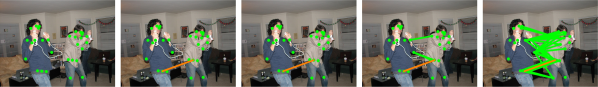
Figure 4: Illustration of inter-human edges with $\epsilon=0^{+},0,100,200,300$ pixels from left to right, where ⁺ means no root-to-root edges. Green points represent body joints. Orange and green lines represent root-to-root edges and $\epsilon$-controlled edges separately.

Table 5: Ablation for inter-human edges on the 3DPW (MPVPE) and MuPoTS ($D\%$). ⁺ means no root-to-root edges.

$\epsilon$	0+	0	100	200	300
MPVPE	113.4	109.2	107.0	106.2	115.1
$D\%$	78.6	89.6	93.2	94.7	90.9

Table 6: Performance of 3DPW with different 2D pose input. P1-3 represent HRNet-32, HRNet-48, and HRNet-48 enhanced by DarkPose separately.

2D Pose	P1	P2	P3	GT
MPVPE	110.3	108.8	106.2	70.1

Inter-human edges: Our method aims at multi-human cases. The core component of our proposed graph structure is the inter-human edges $\mathcal{E}^{\text{Inter}}$, connecting different human subgraphs. We study how inter-human edges affect the performance. As mentioned in Subsection 3.1, root-joints are connected to form root-to-root edges. Also, joint pairs are connected if the pair’s 2D distance in the image is less than $\epsilon$, where the image is preprocessed (resizing the raw image’s long edge as 1000 pixels). A larger $\epsilon$ leads to more dense inter-human edges. In this ablation study, we set $\epsilon=0,100,200,300$ pixels separately. With $\epsilon=0$, $\mathcal{E}^{\text{Inter}}$ only has root-to-root edges. When we remove the root-to-root edges, the whole graph is just the combination of separate subgraphs, which we denote as $\epsilon=0^{+}$. Figure 4 gives an example to show the inter-human edges with different $\epsilon$. Table 6 reports the experiment result. Row two shows the experiments on 3DPW test set with MPVPE as the metric. $\epsilon=0^{+}$ gets 113.4mm MPVPE. With more edges, the performance increases. However, when $\epsilon$ is over 200, connections become too dense, which will hurt the performance. Moreover, we follow [29] to conduct experiments on the MuPoTS-3D dataset to evaluate the ordinal depth relations of all human instance pairs (row three). The number is the percentage of correct depth relations ($D\%$), reflecting the performance of the relative 3D position. If we do not use inter-human edges, the performance is limited, just $78.6\%$, because the information cannot transmit across humans to analyze the relative 3D positions. When we add the root-to-root edges, the accuracy jumps from $78.6\%$ to $89.6\%$, demonstrating the effectiveness of root-to-root edges in model inter-human relations. With larger $\epsilon$, the performance can be better. $\epsilon=200$ produces the best result.

2D pose input: Although we add synthetic error [30, 4] to the 2D pose input in training, making MUG more robust to wrong 2D poses. Input pose with different accuracy can still cause different performances in inference. This ablation experiment explores how various pose inputs affect MUG. We evaluate on 3DPW test set with MPVPE as the metric. We employ three variants of HRNet to produce pose input – HRNet-32, HRNet-48, and HRNet-48 enhanced by DarkPose. The three variants get better 2D pose predictions one by one. Table 6 shows that we can get better human mesh reconstruction results with better pose estimation results as input. Then we compare them with the ground truth input. We observe a significant performance gap boost – the ground truth pose input results in the $34.0\%$ MPJPE drop (from 106.2mm to 70.1mm). The performance of MUG still has much room to increase if we can get a more accurate 2D pose input in testing.

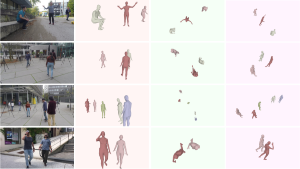
Figure 5: Qualitative results. We show the multi-human mesh reconstruction of MUG on MuPoTS and 3DPW dataset. The second to the forth column are the front, top, side view respectively.

5 Conclusions and Future Work

We studied multi-human mesh reconstruction using 2D pose as input. We designed a multi-layer heterogeneous graph to represent the intra-human and inter-human relations. We further proposed a dual-branch graph neural network that leverages the heterogeneous graph to learn human relations and accurately recovers the 3D mesh coordinates. In the future, we will extend our pipeline for other 3D reconstruction problems, such as animal mesh reconstruction. We hope that this work might spark further use of graph neural networks across various fields within artificial intelligence, such as neural network compression [50].

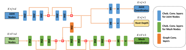
Figure 1: Detailed network structure. The number inside each graph convolution layer represents the feature dimension of the layer output.

Supplementary Material

Appendix 0.A The node feature dimension

MUG applies the joint set from Human3.6M [12] for the experiment on Human3.6M, where $J=17$. The feature dimension of each joint node is

$$d=2+2*17+2+3*11=71\;,$$ (1)

where $2,2*17,2,3*11$ correspond to $\widetilde{P}_{ij}^{\text{2D}},\widetilde{P}_{i}^{\text{2D}},\overline{P}_{ij}^{\text{2D}},(\mathcal{J}T)_{j}$ in the main text respectively. Following the similar calculation, we can also get the feature dimension of each mesh node is $71$. Considering $K$ humans in total and $V=431$, the shape of the joint features is $K\times 17\times 71$ and the shape of the mesh features is $K\times 431\times 71$.

MUG applies COCO [23] joint set for the experiments on Panoptic [14], MuPoTS-3D [27] and 3DPW [25]. Following [4], we add root-joint and neck-joint by computing the middle point of left and right hips, and left and right shoulders respectively. We have $J=19$ for COCO joint set. The feature dimension of each joint or mesh node is

$$d=2+2*19+2+3*11=75\;,$$ (2)

Considering $K$ humans in total and $V=431$, the shape of the joint features is $K\times 19\times 75$ and the shape of the mesh features is $K\times 431\times 75$.

Appendix 0.B Detailed network structure

The detailed network structure is illustrated in Figure 1. The number inside each graph convolution layer represents the feature dimension of the layer output. We adopt the GCN residual block, which is inspired by [10]. Our residual block is similar to the basic residual block of [10]. However, we use Chebyshev spectral graph convolution layers [5] as the convolutional layers and group normalization as the normalization layers.

Appendix 0.C Loss functions

Following [47], the equations for the mesh normal vector loss $L_{\text{N}}$ and mesh edge vector loss $L_{\text{N}}$ are,

$$L_{\text{N}}=\sum_{f}{\sum_{\{a,b\}\subset f}{|<\frac{M_{a}-M_{b}}{\lVert M_{a}-M_{b}\rVert_{2}},n_{f}^{*}>|}}\;,$$ (3)

$$L_{\text{E}}=\sum_{f}{\sum_{\{a,b\}\subset f}{|\lVert M_{a}-M_{b}\rVert_{2}-\lVert M^{*}_{a}-M^{*}_{b}\rVert_{2}|}}\;,$$ (4)

where $f$ and $n_{f}^{*}$ denote a triangle face in the human mesh and a ground truth unit normal vector of $f$, respectively. $M_{a}$ and $M_{b}$ denote the $a^{th}$ and $b^{th}$ ground truth vertices in $f$, respectively. ^∗ represents the ground truth.

Appendix 0.D More qualitative results on MuPoTS

More examples on the MuPoTS dataset are displayed in Figure 2.

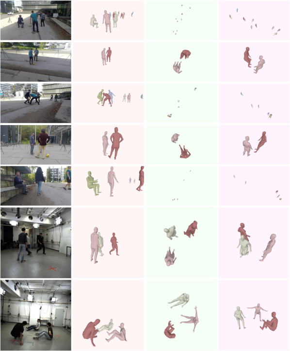
Figure 2: More qualitative results on MuPoTS. The second to the forth column are the front, top, side view respectively.

Appendix 0.E More qualitative results on 3DPW

More examples on the 3DPW dataset are displayed in Figure 3.

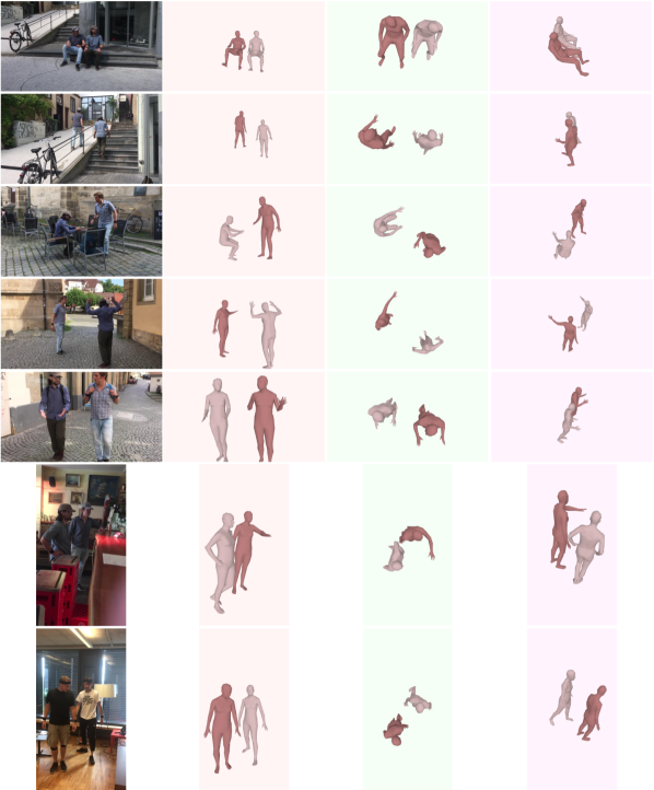
Figure 3: More qualitative results on 3DPW. The second to the forth column are the front, top, side view respectively.

References

- [1] Andriluka, M., Pishchulin, L., Gehler, P., Schiele, B.: 2d human pose estimation: New benchmark and state of the art analysis. In: Proceedings of the IEEE Conference on computer Vision and Pattern Recognition. pp. 3686–3693 (2014)
- [2] Bogo, F., Kanazawa, A., Lassner, C., Gehler, P., Romero, J., Black, M.J.: Keep it SMPL: Automatic estimation of 3D human pose and shape from a single image. In: Proceedings of the European Conference on Computer Vision. pp. 561–578. Springer (2016)
- [3] Cao, Z., Simon, T., Wei, S.E., Sheikh, Y.: Realtime multi-person 2d pose estimation using part affinity fields. In: Proceedings of the IEEE conference on computer vision and pattern recognition. pp. 7291–7299 (2017)
- [4] Choi, H., Moon, G., Lee, K.M.: Pose2Mesh: Graph convolutional network for 3D human pose and mesh recovery from a 2D human pose. In: Proceedings of the European Conference on Computer Vision. pp. 769–787. Springer (2020)
- [5] Defferrard, M., Bresson, X., Vandergheynst, P.: Convolutional neural networks on graphs with fast localized spectral filtering. Advances in neural information processing systems 29, 3844–3852 (2016)
- [6] Fusiello, A.: Elements of geometric computer vision. Available from: http://homepages.inf.ed.ac.uk/rbf/CVonline/LOCAL\_COPIES/FUSIELLO4/tutorial.html (2006)
- [7] Gong, K., Zhang, J., Feng, J.: Poseaug: A differentiable pose augmentation framework for 3d human pose estimation. In: Proceedings of the IEEE/CVF Conference on Computer Vision and Pattern Recognition. pp. 8575–8584 (2021)
- [8] Hamilton, W.L., Ying, R., Leskovec, J.: Inductive representation learning on large graphs. arXiv preprint arXiv:1706.02216 (2017)
- [9] He, K., Gkioxari, G., Dollár, P., Girshick, R.: Mask R-CNN. In: Proceedings of the IEEE International Conference on Computer Vision. pp. 2961–2969 (2017)
- [10] He, K., Zhang, X., Ren, S., Sun, J.: Deep residual learning for image recognition. In: Proceedings of the IEEE conference on computer vision and pattern recognition. pp. 770–778 (2016)
- [11] Huang, Z., Li, Y.: Fsd: Fully-specialized detector via neural architecture search. arXiv preprint arXiv:2305.16649 (2023)
- [12] Ionescu, C., Papava, D., Olaru, V., Sminchisescu, C.: Human3.6M: Large scale datasets and predictive methods for 3D human sensing in natural environments. IEEE Transactions on Pattern Analysis and Machine Intelligence 36(7), 1325–1339 (2013)
- [13] Jiang, W., Kolotouros, N., Pavlakos, G., Zhou, X., Daniilidis, K.: Coherent reconstruction of multiple humans from a single image. In: Proceedings of the IEEE/CVF Conference on Computer Vision and Pattern Recognition. pp. 5579–5588 (2020)
- [14] Joo, H., Liu, H., Tan, L., Gui, L., Nabbe, B., Matthews, I., Kanade, T., Nobuhara, S., Sheikh, Y.: Panoptic studio: A massively multiview system for social motion capture. In: Proceedings of the IEEE International Conference on Computer Vision. pp. 3334–3342 (2015)
- [15] Kanazawa, A., Black, M.J., Jacobs, D.W., Malik, J.: End-to-end recovery of human shape and pose. In: Proceedings of the IEEE Conference on Computer Vision and Pattern Recognition. pp. 7122–7131 (2018)
- [16] Ke, S.R., Thuc, H.L.U., Lee, Y.J., Hwang, J.N., Yoo, J.H., Choi, K.H.: A review on video-based human activity recognition. Computers 2(2), 88–131 (2013)
- [17] Kipf, T.N., Welling, M.: Semi-supervised classification with graph convolutional networks. arXiv preprint arXiv:1609.02907 (2016)
- [18] Kocabas, M., Athanasiou, N., Black, M.J.: Vibe: Video inference for human body pose and shape estimation. In: Proceedings of the IEEE/CVF Conference on Computer Vision and Pattern Recognition. pp. 5253–5263 (2020)
- [19] Kolotouros, N., Pavlakos, G., Black, M.J., Daniilidis, K.: Learning to reconstruct 3D human pose and shape via model-fitting in the loop. In: Proceedings of the IEEE/CVF International Conference on Computer Vision. pp. 2252–2261 (2019)
- [20] Kolotouros, N., Pavlakos, G., Daniilidis, K.: Convolutional mesh regression for single-image human shape reconstruction. In: Proceedings of the IEEE/CVF Conference on Computer Vision and Pattern Recognition. pp. 4501–4510 (2019)
- [21] Li, M., Chen, S., Chen, X., Zhang, Y., Wang, Y., Tian, Q.: Actional-structural graph convolutional networks for skeleton-based action recognition. In: Proceedings of the IEEE/CVF Conference on Computer Vision and Pattern Recognition. pp. 3595–3603 (2019)
- [22] Lin, K., Wang, L., Liu, Z.: End-to-end human pose and mesh reconstruction with transformers. In: Proceedings of the IEEE/CVF Conference on Computer Vision and Pattern Recognition. pp. 1954–1963 (2021)
- [23] Lin, T.Y., Maire, M., Belongie, S., Hays, J., Perona, P., Ramanan, D., Dollár, P., Zitnick, C.L.: Microsoft COCO: Common objects in context. In: Proceedings of the European Conference on Computer Vision. pp. 740–755. Springer (2014)
- [24] Loper, M., Mahmood, N., Romero, J., Pons-Moll, G., Black, M.J.: Smpl: A skinned multi-person linear model. ACM transactions on graphics (TOG) 34(6), 1–16 (2015)
- [25] von Marcard, T., Henschel, R., Black, M.J., Rosenhahn, B., Pons-Moll, G.: Recovering accurate 3d human pose in the wild using imus and a moving camera. In: Proceedings of the European Conference on Computer Vision (ECCV). pp. 601–617 (2018)
- [26] Martinez, J., Hossain, R., Romero, J., Little, J.J.: A simple yet effective baseline for 3D human pose estimation. In: Proceedings of the IEEE International Conference on Computer Vision. pp. 2640–2649 (2017)
- [27] Mehta, D., Rhodin, H., Casas, D., Fua, P., Sotnychenko, O., Xu, W., Theobalt, C.: Monocular 3D human pose estimation in the wild using improved cnn supervision. In: Proceedings of the International Conference on 3D Vision (3DV). pp. 506–516. IEEE (2017)
- [28] Mehta, D., Sotnychenko, O., Mueller, F., Xu, W., Sridhar, S., Pons-Moll, G., Theobalt, C.: Single-shot multi-person 3D pose estimation from monocular RGB. In: Proceedings of the International Conference on 3D Vision (3DV). pp. 120–130. IEEE (2018)
- [29] Moon, G., Chang, J.Y., Lee, K.M.: Camera distance-aware top-down approach for 3D multi-person pose estimation from a single RGB image. In: Proceedings of the IEEE/CVF International Conference on Computer Vision. pp. 10133–10142 (2019)
- [30] Moon, G., Chang, J.Y., Lee, K.M.: Posefix: Model-agnostic general human pose refinement network. In: Proceedings of the IEEE/CVF Conference on Computer Vision and Pattern Recognition. pp. 7773–7781 (2019)
- [31] Moon, G., Lee, K.M.: I2L-MeshNet: Image-to-lixel prediction network for accurate 3D human pose and mesh estimation from a single RGB image. arXiv preprint arXiv:2008.03713 (2020)
- [32] Paszke, A., Gross, S., Massa, F., et al.: Pytorch: An imperative style, high-performance deep learning library. In: Advances in Neural Information Processing Systems 32, pp. 8024–8035. Curran Associates, Inc. (2019), https://pytorch.org
- [33] Pavlakos, G., Choutas, V., Ghorbani, N., Bolkart, T., Osman, A.A., Tzionas, D., Black, M.J.: Expressive body capture: 3D hands, face, and body from a single image. In: Proceedings of the IEEE/CVF Conference on Computer Vision and Pattern Recognition. pp. 10975–10985 (2019)
- [34] Pavlakos, G., Zhu, L., Zhou, X., Daniilidis, K.: Learning to estimate 3D human pose and shape from a single color image. In: Proceedings of the IEEE Conference on Computer Vision and Pattern Recognition. pp. 459–468 (2018)
- [35] Ranjan, A., Bolkart, T., Sanyal, S., Black, M.J.: Generating 3d faces using convolutional mesh autoencoders. In: Proceedings of the European Conference on Computer Vision (ECCV). pp. 704–720 (2018)
- [36] Ren, S., He, K., Girshick, R., Sun, J.: Faster r-cnn: Towards real-time object detection with region proposal networks. Advances in Neural Information Processing Systems 28, 91–99 (2015)
- [37] Schlichtkrull, M., Kipf, T.N., Bloem, P., Van Den Berg, R., Titov, I., Welling, M.: Modeling relational data with graph convolutional networks. In: Proceedings of the European Semantic Web Conference. pp. 593–607. Springer (2018)
- [38] Sigal, L., Balan, A.O., Black, M.J.: Humaneva: Synchronized video and motion capture dataset and baseline algorithm for evaluation of articulated human motion. International journal of computer vision 87(1-2), 4 (2010)
- [39] Sun, K., Xiao, B., Liu, D., Wang, J.: Deep high-resolution representation learning for human pose estimation. In: Proceedings of the IEEE/CVF Conference on Computer Vision and Pattern Recognition. pp. 5693–5703 (2019)
- [40] Sun, Y., Bao, Q., Liu, W., Fu, Y., Black, M.J., Mei, T.: Monocular, one-stage, regression of multiple 3d people. In: Proceedings of the IEEE/CVF International Conference on Computer Vision. pp. 11179–11188 (2021)
- [41] Tobler, W.R.: A computer movie simulating urban growth in the detroit region. Economic geography 46(sup1), 234–240 (1970)
- [42] Veličković, P., Cucurull, G., Casanova, A., Romero, A., Lio, P., Bengio, Y.: Graph attention networks. arXiv:1710.10903 (2017)
- [43] Wandt, B., Rosenhahn, B.: Repnet: Weakly supervised training of an adversarial reprojection network for 3d human pose estimation. In: Proceedings of the IEEE/CVF Conference on Computer Vision and Pattern Recognition. pp. 7782–7791 (2019)
- [44] Wang, J.Z., Badler, N., Berthouze, N., Gilmore, R.O., Johnson, K.L., Lapedriza, A., Lu, X., Troje, N.: Bodily expressed emotion understanding research: A multidisciplinary perspective. In: Proceedings of the First International Workshop on Bodily Expressed Emotion Understanding, in conjunction with the European Computer Vision Conference. pp. 733–746 (2020)
- [45] Wang, L., Chen, Y., Guo, Z., Qian, K., Lin, M., Li, H., Ren, J.S.: Generalizing monocular 3d human pose estimation in the wild. In: Proceedings of the IEEE/CVF International Conference on Computer Vision Workshops. pp. 0–0 (2019)
- [46] Wang, M., Zheng, D., Ye, Z., Gan, Q., Li, M., Song, X., Zhou, J., Ma, C., Yu, L., Gai, Y., Xiao, T., He, T., Karypis, G., Li, J., Zhang, Z.: Deep graph library: A graph-centric, highly-performant package for graph neural networks. arXiv preprint arXiv:1909.01315 (2019)
- [47] Wang, N., Zhang, Y., Li, Z., Fu, Y., Liu, W., Jiang, Y.G.: Pixel2Mesh: Generating 3D mesh models from single RGB images. In: Proceedings of the European Conference on Computer Vision. pp. 52–67 (2018)
- [48] Wang, X., Ji, H., Shi, C., Wang, B., Ye, Y., Cui, P., Yu, P.S.: Heterogeneous graph attention network. In: The World Wide Web Conference. pp. 2022–2032 (2019)
- [49] Wu, C., Chen, Y., Luo, J., Su, C.C., Dawane, A., Hanzra, B., Deng, Z., Liu, B., Wang, J.Z., Kuo, C.h.: Mebow: Monocular estimation of body orientation in the wild. In: Proceedings of the IEEE/CVF Conference on Computer Vision and Pattern Recognition (CVPR) (June 2020)
- [50] Xu, Y., Dong, X., Li, Y., Su, H.: A main/subsidiary network framework for simplifying binary neural networks. In: Proceedings of the IEEE/CVF Conference on Computer Vision and Pattern Recognition (CVPR) (June 2019)
- [51] Yang, Y., Qiu, J., Song, M., Tao, D., Wang, X.: Distilling knowledge from graph convolutional networks. In: Proceedings of the IEEE/CVF Conference on Computer Vision and Pattern Recognition. pp. 7074–7083 (2020)
- [52] Yu, W., Huang, Z., Zhang, W., Feng, L., Xiao, N.: Gradual network for single image de-raining. In: Proceedings of the 27th ACM international conference on multimedia. pp. 1795–1804 (2019)
- [53] Zanfir, A., Marinoiu, E., Sminchisescu, C.: Monocular 3D pose and shape estimation of multiple people in natural scenes-the importance of multiple scene constraints. In: Proceedings of the IEEE Conference on Computer Vision and Pattern Recognition. pp. 2148–2157 (2018)
- [54] Zanfir, A., Marinoiu, E., Zanfir, M., Popa, A.I., Sminchisescu, C.: Deep network for the integrated 3D sensing of multiple people in natural images. Advances in Neural Information Processing Systems 31, 8410–8419 (2018)
- [55] Zhang, F., Zhu, X., Dai, H., Ye, M., Zhu, C.: Distribution-aware coordinate representation for human pose estimation. In: Proceedings of the IEEE/CVF conference on computer vision and pattern recognition. pp. 7093–7102 (2020)
- [56] Zhang, J., Yu, D., Liew, J.H., Nie, X., Feng, J.: Body meshes as points. arXiv preprint arXiv:2105.02467 (2021)
- [57] Zhou, X., Huang, Q., Sun, X., Xue, X., Wei, Y.: Towards 3d human pose estimation in the wild: A weakly-supervised approach. In: The IEEE International Conference on Computer Vision (ICCV) (Oct 2017)