Optimized mitigation of random-telegraph-noise dephasing
by spectator-qubit sensing and control

Abstract

Spectator qubits (SQs) are a tool to mitigate noise in hard-to-access data qubits. The SQ, designed to be much more sensitive to the noise, is measured frequently, and the accumulated results used rarely to correct the data qubits. For the hardware-relevant example of dephasing from random telegraph noise, we introduce a Bayesian method employing complex linear maps which leads to a plausibly optimal adaptive measurement and control protocol. The suppression of the decoherence rate is quadratic in the SQ sensitivity, establishing that the SQ paradigm works arbitrarily well in the right regime.

Despite recent impressive advances towards large-scale quantum computing Arute et al. (2019); Zhong et al. (2020), the challenge of suppressing noise sufficiently to achieve scalable universal quantum computing remains Temme et al. (2017); Preskill (2018); Endo et al. (2018); Kandala et al. (2019). The best known approaches to noise-mitigation are dynamical decoupling (DD), which works for non-Markovian noise Viola et al. (1999); Viola and Knill (2003); Biercuk et al. (2011); Ng et al. (2011); Souza et al. (2011); Medford et al. (2012); Paz-Silva and Lidar (2013); Zhang et al. (2014), and quantum encoding and error correction (QEC) which works best for Markovian and local noise Shor (1995); Steane (1996); Terhal (2015). In favourable regimes, both of these approaches can suppress errors arbitrarily.

For data qubits that are very well isolated from their environment, it could be difficult to control them (as for DD) or measure them (for QEC) rapidly. In this context, another paradigm for error mitigation has recently been proposed and demonstrated Gupta et al. (2020); Majumder et al. (2020); Singh et al. (2022): spectator qubits (SQs). The SQ is located physically near to the data qubits. It is a spectator in two senses: it does not interact with the data qubits, but it is a sensitive probe to the noise they experience. The idea is that by measuring the SQ in a suitable way, the experimenter can obtain information about the noise in real time, and, by applying suitable controls, cancel at least some of the effect of that noise on the data qubits.

Previous work within the SQ paradigm has used rather simple measurement and control strategies, and has not shown that the SQ can, like DD and QEC, work arbitrarily well in a suitable regime. In this Letter, we transform that situation. We consider an experimentally relevant type noise that effects many qubits: dephasing caused by a random telegraph process (RTP) Itakura and Tokura (2003); Galperin et al. (2006); Culcer et al. (2009); Bergli et al. (2009). We consider the regime where the flip-rates, $\gamma_{\uparrow}$, $\gamma_{\downarrow}$, of the RTP are large compared to $\kappa$, the data qubit’s sensitivity to the RTP, but small compared to the SQ’s sensitivity, $K$:

$$T^{-1},~{}\kappa\ll\gamma_{\uparrow,\downarrow}\ll K.$$ (1)

Here $T$ is the time at which the control is applied on the data qubit. We introduce a principled method, based on Bayesian maps, to construct a measurement and control algorithm that is, we conjecture, optimal in this regime. Our algorithm suppresses the data qubit decoherence by an amount (i.e., a divisor) scaling as $(K/\bar{\gamma})^{2}$, where $\bar{\gamma}:=(\gamma_{\uparrow}+\gamma_{\downarrow})/2$, limited only by the sensitivity of the SQ.

We tackle the problem from the perspective of quantum estimation or decision theory Helstrom (1976); Wiseman and Milburn (2010). The ultimate limits to such problems are surprisingly subtle even with a single probe qubit confined to a single plane Acín et al. (2005); Higgins et al. (2009, 2011); Slussarenko et al. (2017); Martínez Vargas et al. (2021); Sergeevich et al. (2011); Ferrie et al. (2013); Shulman et al. (2014); Sekatski et al. (2017). In all of these, the optimal sequence of single-qubit measurements is, in general, adaptive; that is, the basis for later measurements must depend on the results of earlier measurements Wiseman and Milburn (2010); Sergeevich et al. (2011); Shulman et al. (2014). The SQ problem we consider here is more complicated than the above examples Acín et al. (2005); Higgins et al. (2009, 2011); Slussarenko et al. (2017); Martínez Vargas et al. (2021); Sergeevich et al. (2011); Ferrie et al. (2013); Shulman et al. (2014); Sekatski et al. (2017) in three ways. First, it is dynamic: there is a Hamiltonian affecting the qubit rotation that changes stochastically (the RTP). Second, we allow a choice not just in the time of application of the Hamiltonian before measurement (as in Sergeevich et al. (2011)), but also in the measurement basis. Third, the quantity to be estimated is not the current state of the SQ, nor even the current state of the RTP (i.e. the current Hamiltonian). Rather, it is the cumulative phase acquired by the data qubit, proportional to the integral of the RTP up to that time.

In this Letter, we show that, despite these complications, it is possible, in the relevant regime (1), to derive a measurement and control strategy using the SQ that is plausibly optimal. That is, in the multiplicative factor by which the data qubit decoherence rate is reduced,

$$H^{\star}\,(\bar{\gamma}/K)^{2},\text{ where }H^{\star}\approx 1.254,$$ (2)

even the prefactor ($H^{\star}$) is as small as possible. Unsurprisingly, we find that the optimized strategy is adaptive.

Finding the ultimate limit to a harder qubit-probe estimation problem than has hitherto been considered serves as a benchmark against which other techniques, such as machine learning, can be compared. Having an optimal SQ protocol solution could help to hone heuristic algorithms for even more complicated problems.

The structure of this paper is as follows. First we introduce the physical system: the RTP, the data qubit, and the SQ (see Fig. 1). Next we introduce the calculational tool of Bayesian maps. Then we consider a greedy algorithm, and, with insights from that, construct the optimized algorithm that achieves (2), and verify it numerically. We conclude with open problems. More details in all sections are found in the companion paper (CP) Tonekaboni et al. (2022).

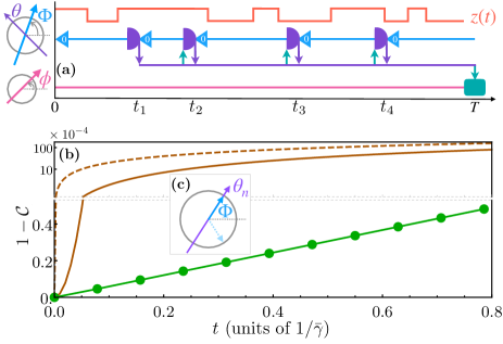
Figure 1: (a) Schema for the SQ protocol, showing dynamics of (from top to bottom): RTP (orange); SQ (blue) which is reprepared (triangle) after each measurement (purple semi-circle and downward arrows); measurement record (purple); and data qubit (pink). Teal arrows from measurement record show feedback (upwards for adaptive measurements on the SQ and downward to the teal box at $t=T$ representing the final control on the data qubit). Small Bloch spheres at left indicate the meaning of $\theta$, $\Phi$, and $\phi$. (b) Plot of data qubit decoherence ($1-\mathcal{C}$) versus $t$, with change to log-scale for $1-\mathcal{C}>0.55\times 10^{-4}$. From top to bottom: no-control asymptotic result, Eq. (6), dashed brown; exact no-control case, solid brown; exact Greedy algorithm data points with fit (green). Parameters: $\kappa=0.2,\gamma_{\uparrow}=\gamma_{\downarrow}=1,K=20$. (c) Bloch sphere showing how Greedy chooses the measurement axis $\theta_{n}$ to align with the most likely SQ state, $|{\Phi}\rangle^{\rm s}$.

I Charge noise and RTP

One of the main causes of decoherence for solid-state qubits is the stochastic motion of particles in traps in oxide layers or interfaces  Zorin et al. (1996); Paladino et al. (2002); Itakura and Tokura (2003); Galperin et al. (2006); Culcer et al. (2009); Bergli et al. (2009). The simplest model capturing the essential physics of such processes is the RTP $z(t)$, which has a Lorentzian noise spectrum. The RTP switches between two values: $z_{t}:=z(t)=\pm 1$. Defining $\underline{P}_{t}=\left(\wp(z_{t}=+1),\wp(z_{t}=-1)\right)\!^{\top}$ as the vector of probabilities at any given time, the master equation, and its steady state (ss) distribution, are, respectively Gardiner (1985)

$$\underline{{\dot{P}}}_{t}=\left(\begin{matrix}-\gamma_{\downarrow}&+\gamma_{\uparrow}\\ +\gamma_{\downarrow}&-\gamma_{\uparrow}\end{matrix}\right)\underline{{P}}_{t}\;\;{\rm and}\;\;\underline{{P}}_{\rm ss}=\frac{1}{2\bar{\gamma}}\left(\begin{matrix}\gamma_{\uparrow}\\ \gamma_{\downarrow}\end{matrix}\right),$$ (3)

where $\bar{\gamma}=(\gamma_{\uparrow}+\gamma_{\downarrow})/2$ as before. For the calculations below, we are also interested in the time-integrated noise,

$$X=\int_{0}^{t}\!z(s){\rm d}s,$$ (4)

where we omit the $t$-dependence when it is not needed. In particular, we need to solve not just for $\wp(z_{t})$ via Eq. (3), but also for $\wp(X,z_{t})$; see the CP Tonekaboni et al. (2022).

II Data qubit dephasing

We assume the data qubit decoherence is caused by phase fluctuation. The coherence remaining at any time can thus be calculated by taking the absolute value of the average of the phasors:

$$\mathcal{C}=\left|\left\langle e^{i\phi(\Xi)}\right\rangle_{\Xi}\right|,$$ (5)

where $\phi$ is the data qubit’s phase and $\Xi$ is all the variables on which $\phi$ depends. (We ignore the dependence on $\phi(0)$ by taking that to be $0$). In this work, we assume the RTP causes the phase fluctuation via the data (d) qubit’s Hamiltonian $\hat{H}_{\rm d}=\frac{\kappa}{2}\,\hat{\sigma}_{z}^{\rm d}z(t)$. Thus $\Xi$ arises from the RTP plus any controls applied to the data qubit.

In the absence of control, we simply have $\Xi={X}$ and $\phi({X})=\kappa\,{X}$, as the data qubit phase just accumulates. In the CP Tonekaboni et al. (2022), we give a closed-form expression for the no-control (nc) coherence, and show that in the long-time limit ($t\gg\breve{\gamma}^{-1}$), the coherence decays exponentially:

$$\tfrac{{\rm d}}{{\rm d}t}\mathcal{C}^{\rm nc}=-\Gamma^{\rm nc}\mathcal{C}^{\rm nc}\;;\quad\Gamma^{\rm nc}=\kappa^{2}\breve{\gamma}/2\bar{\gamma}^{2}.$$ (6)

Here $\breve{\gamma}:=2\gamma_{\uparrow}\gamma_{\downarrow}/(\gamma_{\uparrow}+\gamma_{\downarrow})$ is the harmonic mean of $\gamma_{\uparrow},\gamma_{\downarrow}$.

Say the quantum data is required at some time. If we have additional information, $Y$, about $X$, at that time, then we can increase the coherence $\mathcal{C}$, by controlling the data qubit conditioned on $Y$. Specifically, a unitary $\hat{\sigma}_{z}^{\rm d}$-rotation can add a phase correction, $c(Y)$, to $\phi$. This means that the data qubit phase depends on two variables, $\Xi=({X},Y)$, via $\phi({X},Y)=\kappa{X}-c(Y)$. Of course these two variables are not independent, as $Y$ contains information about $X$. We show in the CP Tonekaboni et al. (2022) that the optimal choice for the control is

$$c(Y)=\arg\mathcal{A}_{|Y},\text{ where }\mathcal{A}_{|Y}:=\left\langle e^{i\kappa{X}}\right\rangle_{{X}|Y}.$$ (7)

That is, whatever information $Y$ exists, this choice of control maximizes the coherence (5). Therefore, if the qubit is needed at time $T$, the appropriate reward function for our problem is $\mathcal{C}^{\rm c}(T)$, where Tonekaboni et al. (2022)

$$\mathcal{C}^{\rm c}:=\left|\left\langle e^{i\phi({X},Y)}\right\rangle_{{X},Y}\right|=\sum_{Y}\wp(Y)\left|\mathcal{A}_{|Y}\right|,$$ (8)

with $\wp(Y)$ being the probability of obtaining the information $Y$. Thus $\left|\mathcal{A}_{|Y}\right|$ can be interpreted as conditional coherence.

III SQ for noise sensing

As motivated in the introduction, a natural way to obtain $Y$ is to use a SQ (s). This is similar to the data qubit but with a Hamiltonian $\frac{K}{2}\hat{\sigma}_{z}^{\rm s}z(t)$ making it more sensitive to the noise than the data qubit ($K\gg\kappa$). It can be frequently probed, as described by a projective measurement of the observable $\mathbb{1}-|{\theta}\rangle^{\rm s}\langle{\theta}|$, yielding outcomes $y\in\{0,1\}$. Here $|{\theta}\rangle^{\rm s}$ is the equatorial state $(|{+1}\rangle^{\rm s}_{z}+e^{i\theta}|{-1}\rangle^{\rm s}_{z})/\sqrt{2}$, with $\hat{\sigma}_{z}^{\rm s}|{\pm 1}\rangle^{\rm s}_{z}=\pm|{\pm 1}\rangle^{\rm s}_{z}$. The SQ is initially prepared in the equatorial state $|{0}\rangle^{\rm s}$, and immediately reset to this after each measurement. Between measurements it remains in an equatorial state, $|{\Phi}\rangle^{\rm s}$, with $\dot{\Phi}(t)=Kz(t)$. See Fig. 1(a).

Let us define $\{t_{1},t_{2},\dots,t_{N}\equiv T\}$ as the times for SQ measurement and $y_{n}\in\{0,1\}$ as the corresponding measurement results. At any $t_{n}$, the SQ phase accumulated during the waiting time $\tau_{n}:=t_{n}-t_{n-1}$, between measurements, is $\Phi(t_{n})=Kx_{n}$, where $x_{n}:=X(t_{n})-X(t_{n-1})$ from Eq. (4). We use Bayesian estimation and control based on the likelihood function

$$\wp(y_{n}|\theta_{n},x_{n})=\left|y_{n}-\cos^{2}\left[{\mbox{$\frac{1}{2}$}(\theta_{n}-Kx_{n})}\right]\right|,$$ (9)

where $\theta_{n}$ is the equatorial measurement angle introduced above at time $t_{n}$.Now, given the record $Y_{n}:=(y_{1},y_{2},\dots,y_{n})$, with $n\leq N$, the problem is to optimize the choice for the next waiting time $\tau_{n+1}$ and measurement angle $\theta_{n+1}$ to maximize the reward function (8). (Note that when we condition on $Y_{n}$ we implicitly condition on all the previous choices of durations and angles which are functions of the earlier parts of $Y_{n}$.) This optimization requires us to better understand Eq. (8).

IV Bayesian maps for phase estimation

We show in the CP Tonekaboni et al. (2022) that, from the dynamics of the RTP described in Eqs. (3) and (4), and the likelihood function (9), we can apply Bayes’ theorem to evaluate Eq. (8) at $t=T$ as

$$\mathcal{C}^{\rm c}(T)=\sum\nolimits_{Y_{N}}\left|\wp(Y_{N})\mathcal{A}_{|Y_{N}}\right|=\sum\nolimits_{Y_{N}}\left|\underline{I}^{\top}\,\underline{A}_{N}\right|.$$ (10)

Here $\underline{I}=\left(1,1\right)^{\top}$, while we define $\underline{A}_{n}$ for any $n$ as

$$\underline{A}_{n}=(A^{+1}_{n},A^{-1}_{n})^{\top},\textrm{ where }A^{z_{n}}_{n}:=\wp(Y_{n},z_{n})\mathcal{A}_{|Y_{n},z_{n}},$$

and $z_{n}:=z(t_{n})$. This can be efficiently calculated via

$$\underline{{A}}_{n}={\bf F}(\theta_{n},\tau_{n},y_{n})\,\cdots\,{\bf F}(\theta_{1},\tau_{1},y_{1})\,\underline{A}_{0},$$ (11)

where each ${\bf F}(\theta,\tau,y)$ is a $2\times 2$ complex matrix (one for each measurement), which also depends upon $\kappa$, $\gamma_{\uparrow}$, $\gamma_{\downarrow}$, and $K$. Here, $\underline{A}_{0}=\underline{{P}}_{0}$ encodes the initial or prior probabilities for $z_{0}$, which we take to be the unconditioned stationary probabilities $\underline{{P}}_{\text{ss}}$ of Eq. (3). The optimal final data qubit control in Eq. (7) can thus also be easily computed in an experiment as $c(Y_{N})=\arg(\underline{I}^{\top}\,\underline{A}_{N})$. The full expression for ${\bf F}$ is lengthy and is given in the CP Tonekaboni et al. (2022).

Recall that the task is to choose $\tau_{n+1}$ and $\theta_{n+1}$ given $Y_{n}$ so as to maximize $\mathcal{C}^{\rm c}(T)$. The significance of Eqs. (10) and (11) is that the choice should depend only on $\underline{{A}}_{n}$ Tonekaboni et al. (2022). Although $\underline{{A}}_{n}$, a complex 2-vector, encodes four real parameters, it can be shown Tonekaboni et al. (2022) there are only two real sufficient statistics for the adaptive measurement choice, which we now define and explain.

If, hypothetically, we could find out $z_{n}$, we could use that to refine the control that we would (hypothetically, if $t_{n}$ were $T$) apply to the data qubit, from $c_{n}(Y_{n})=\arg\mathcal{A}_{|Y_{n}}$ to $c^{\prime}_{n}(Y_{n},z_{n})=\arg\mathcal{A}_{|Y_{n},z_{n}}$. The difference between the two refined values, $c^{\prime}_{n}(Y_{n},+1)-c^{\prime}_{n}(Y_{n},-1)$, scaled to be typically $O(1)$ Tonekaboni et al. (2022), is

$$\alpha_{n}:=\frac{K}{\kappa}\left({\arg\mathcal{A}_{|Y_{n},+1}-\arg\mathcal{A}_{|Y_{n},-1}}\right)=\frac{K}{\kappa}\arg\frac{A_{n}^{z=+1}}{A_{n}^{z=-1}}.$$ (12)

This $\alpha$ is the first of the two sufficient statistics.

Now, in the limit $\kappa\ll K$, not only are the arguments of $\mathcal{A}_{|Y_{n},\pm 1}$ very close, as per Eq. (12), but so are their moduli, with $|\mathcal{A}_{|Y_{n},+1}|/|\mathcal{A}_{|Y_{n},-1}|=1+O\big{(}(\kappa/K)^{2}\big{)}$ Tonekaboni et al. (2022). It follows, with relative errors of the same magnitude, that $|A_{n}^{z_{n}}|\approx|\mathcal{A}_{|Y_{n}}|\,\wp(Y_{n},z_{n})$, and that

$$\zeta_{n}:=\left({|A_{n}^{z=+1}|-|A_{n}^{z=-1}|}\right)/\left({|A_{n}^{z=+1}|+|A_{n}^{z=-1}|}\right)$$ (13)

is approximately the mean of $z_{n}$ conditioned on $Y_{n}$. This $\zeta$ is the second of the two sufficient statistics.

V Greedy algorithm

The most obvious strategy, for choosing $\tau_{n+1}$ and $\theta_{n+1}$, is a ‘greedy’ one. Given $Y_{n}$ but before $y_{n+1}$ is obtained, ‘Greedy’ (as we call it) at time $t$ acts as if $T=t+{\rm d}t$ (i.e. as if the protocol were about to end) and maximizes the reward function at that time, $\mathcal{C}^{\rm c}_{|Y_{n}}(t+{\rm d}t)$, conditioned on the known information. This is explored in detail in the CP Tonekaboni et al. (2022). We find that, in the regime of Eq. (1), to an excellent approximation, Greedy chooses adaptively, as follows:

$$\theta_{n+1} =s_{n}\Theta_{\rm G}(\alpha_{n},|\zeta_{n}|)\;\text{ where }s_{n}:={\rm sign}(\zeta_{n}),$$ (14)

$$\tau_{n+1} =|\theta_{n+1}|/K.$$ (15)

Here $\Theta_{\rm G}\approx\pi/2$, varying by only $2.5\%$ as its arguments vary. Since $s_{n}$ is the most likely value of $z_{n}$, the choice $\theta_{n+1}=K\tau_{n+1}s_{n}$ corresponds to measuring along the direction of the most likely state $|{\Phi}\rangle^{\rm s}$ of the SQ [Fig. 1(c)], with $y=0$ being the most likely, or ‘null’ result. Naively, one might expect $\Theta_{\rm G}=\pi/2$ to be optimal since, ignoring jumps during the measurement interval, a duration of $\tau=\pi/(2K)$ would map the two RTP states ($z_{n}=\pm 1$) to orthogonal states of the SQ ($\Phi=\pm\pi/2$). However, while Greedy does greatly suppress decoherence [Fig. 1(b)], we can achieve more by optimizing $\Theta$, as we now show.

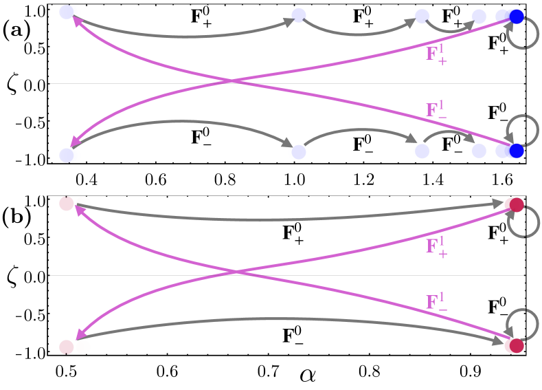
Figure 2: Phase-space ($\zeta,\alpha$) portrait showing jumps induced by measurement maps ${\bf F}_{s}^{y}$ for the constant-$\Theta$ adaptive scheme, with $\Theta=1.0$ (a) and $\Theta=\Theta^{\star}\approx 1.50$ (b). Dots are all possible points after $n=10$ measurements with colour saturation showing relative probability. Parameters are as in Fig. 1.

VI Map-based Optimized Adaptive Algorithm for Asymptotic Regime (MOAAAR)

We use a map-based approach for our optimization, in order to obtain analytical results in the asymptotic regime (1). We make the ansätze (14), (15) for the adaptive algorithm, but replace $\Theta_{\rm G}$ by $\Theta$, a constant. Hence there are only four possible values of the map ${\bf F}(\theta_{n},\tau_{n},y_{n})$ in Eq. (11). These are ${\bf F}^{y}_{s}(\Theta):={\bf F}(s\Theta,\Theta/K,y)$, with $y\in\{0,1\}$ and $s=\pm$. To understand and thus optimize our algorithm, we need to study the behaviour of the parameters $(\alpha,\zeta)$, which encode all our relevant knowledge.

The behaviour is shown in Fig. 2(a), choosing $\Theta=1.0$ for illustrative purposes. Under the mapping (11), applied stochastically with the actual statistics of $Y_{n}$, we see that the ‘system’ $(\alpha,\zeta)$ spends almost all of the time close to just two points. These are the fixed points (stable eigenstates) $\underline{{E}}_{\pm}^{0}$ of the maps ${\bf F}^{0}_{\pm}(\Theta)$ with the null outcome ($y=0$). Thus, if we ignore the initial [$t=O(1/\breve{\gamma})$] and final [$T-t=O(1/\breve{\gamma})$] transients, the dynamics of $(\alpha,\zeta)$ mirrors that of the RTP, with transition rates $\gamma_{\uparrow},\gamma_{\downarrow}$. This is an ergodic process with steady state $P_{\rm ss}$ in Eq. (3).

To maximize Eq. (10) for $T\gg\breve{\gamma}^{-1}$, transients can be ignored. Thus we seek a $\Theta$ that minimizes the decay of $\mathcal{C}^{\rm c}(t)$ in the ergodic regime. Consider first the relative change, $\delta$, in the conditional coherence, $|\mathcal{A}_{|Y_{n}}|$. As the system state evolves from a known $\underline{{A}}_{n}$ at time $t_{n}$ to an unknown one at time $t_{n+1}=t_{n}+\tau$, this is given by

$$\delta(\underline{{A}}_{n}) :=\left[\left|\mathcal{A}_{|Y_{n}}\right|-\sum_{y_{n+1}}\wp(y_{n+1}|Y_{n})\left|\mathcal{A}_{|Y_{n+1}}\right|\right]/\left|\mathcal{A}_{|Y_{n}}\right|$$

$$=1-|\underline{I}^{\top}\underline{A}_{n}|^{-1}\sum\nolimits_{y}|\underline{I}^{\top}\,{\bf F}_{s_{n}}^{y}\!(\Theta)\,\underline{A}_{n}|.$$ (16)

From the above considerations of ergodicity, it can be shown Tonekaboni et al. (2022) that the decay rate $\bar{\Gamma}$ of $\mathcal{C}^{\rm c}$ can be evaluated as $\bar{\delta}/\tau$, where the bar indicates the steady-state ensemble average. That is, emphasising the $\Theta$-dependence,

$$\bar{\Gamma}(\Theta):=\sum_{s=\pm}{P}_{\rm ss}(s)\frac{|\underline{I}^{\top}\underline{E}_{s}^{0}|-\sum_{y}|\underline{I}^{\top}\,{\bf F}_{s}^{y}(\Theta)\,\underline{E}_{s}^{0}|}{\tau|\underline{I}^{\top}\underline{E}_{s}^{0}|}.$$ (17)

Finally, a lengthy calculation Tonekaboni et al. (2022) reveals that in the regime (1), $\bar{\Gamma}(\Theta)\to H_{\Theta}\breve{\gamma}\kappa^{2}/(2K^{2})$, where $H_{\Theta}$ equals

$$3\Theta^{2}\csc^{4}\Theta-[2\Theta(\Theta-\cot\Theta)+1]{\rm csc}^{2}\Theta+\tfrac{1}{3}\Theta^{2}-1.$$ (18)

This function is plotted in the inset of Fig. 3.

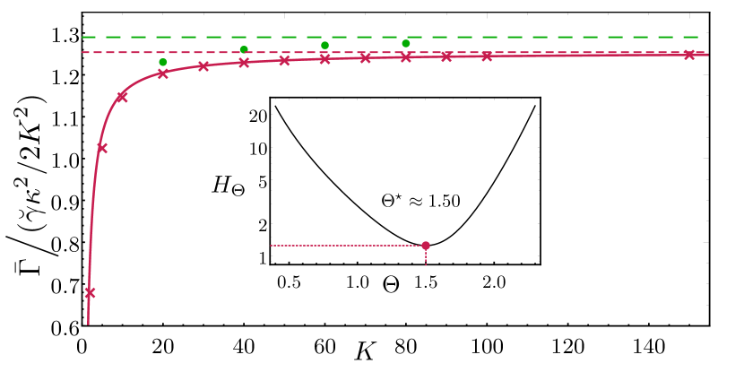
Figure 3: Decoherence rate for Greedy (green dots) and MOAAAR (maroon crosses) versus $K$, scaled so as to asymptote to $O(1)$, with $\kappa=0.2,\gamma_{\uparrow}=\gamma_{\downarrow}=1$. Data points are from slope-fitting to exact numerical calculations of Eq. (8). Asymptotes (horizontal, dashed) are from Eq. (18) (plotted in the inset), with $\Theta=\pi/2$ (Greedy, green long dashes) and $\Theta=\Theta^{\star}$ (MOAAAR, maroon short dashes). Curve (solid) for MOAAAR is a closed-form approximation in the CP Tonekaboni et al. (2022).

Its minimum is $H^{\star}\approx 1.254$ at $\Theta=\Theta^{\star}\approx 1.50055$. This optimization defines our MOAAAR protocol, the one giving the minimum decoherence rate of $\bar{\Gamma}(\Theta^{\star})=H^{\star}{\breve{\gamma}\kappa^{2}}/(2K^{2}).$ Comparing with the no-control case (6), gives the earlier quoted quadratic decoherence suppression, Eq. (2).

We show the dynamics of phase space ($\alpha,\zeta$) for $\Theta=\Theta^{\star}$ in Fig. 2(b). As expected, the system spends almost all its time in the two fixed points $E^{0}_{\pm}$, until a non-null result ($y=1$) causes a jump to ${\bf F}^{1}_{\pm}E^{0}_{\pm}$. But, unlike in Fig. 2(a) ($\Theta=1.0$), at the next measurement the system almost always jumps practically the whole way back to a fixed point $E^{0}_{\mp}$ (the opposite one whence it started). Thus the entire evolution is, for all practical purposes, confined to four points, $E^{0}_{\pm}$ and ${\bf F}^{1}_{\pm}E^{0}_{\pm}$.

The fact that $\Theta^{\star}$ is significantly different from $\pi/2$ (as chosen by Greedy almost all the time in the asymptotic limit), highlights the nontriviality of MOAAAR. It also means that to implement MOAAAR experimentally would require a real-time feedback loop, albeit quite a simple one: one simply switches the sign of $\theta$ whenever a non-null result ($y=1$) is obtained. In Fig. 3 we confirm by exact numerics that MOAAAR outperforms Greedy and that their decoherence rates, scaled by $2K^{2}/(\breve{\gamma}\kappa^{2})$, asymptote to $H^{\star}$ and $H_{\pi/2}\approx 1.290$ respectively. In the CP Tonekaboni et al. (2022) we provide further evidence supporting the plausibility of the optimality of MOAAAR, by showing numerically that it is also the optimal algorithm out of a larger family of algorithms. Specifically, we optimize over two parameters, $\Theta$ and $\tau$, where $\tau$ is fixed but not constrained by $\tau=\Theta/K$.

VII Discussion

For suppression of RTP phase noise, using information obtained from a SQ, we have proposed a protocol (MOAAAR) — an adaptive sequence of projective measurements on the SQ, followed by a control on the data qubit at the final time — which is plausibly optimal in the good parameter regime. In this regime, the suppression of the decoherence rate, Eq. (2), is limited only by the SQ sensitivity. A conceptually simpler but implementationally more complicated algorithm, ‘Greedy’, performs slightly worse. In the CP Tonekaboni et al. (2022) we perform further comparisons of these two strategies.

This work establishes that, like the well-known noise-mitigation strategies of DD and QEC, the SQ paradigm can work arbitrarily well in a suitable regime. The approach we use here can certainly be generalized for more complicated noise processes, such as multiple RTPs or multi-level RTPs. This, and other directions to study the applicability of SQs in real-world situations, are discussed in the CP Tonekaboni et al. (2022).