Continuum Skyrme Hartree-Fock-Bogoliubov theory with Green’s function method
for neutron-rich Ca, Ni, Zr, Sn isotopes

Abstract

The possible exotic nuclear properties in the neutron-rich Ca, Ni, Zr, and Sn isotopes are explored with the continuum Skyrme Hartree-Fock-Bogoliubov theory formulated with the Green’s function method, in which the pairing correlation, the couplings with the continuum, and the blocking effects for the unpaired nucleon in odd-$A$ nuclei are properly treated. In the $ph$ channel, the SLy4 parameter set is taken for the Skyrme interaction, and in the $pp$ channel, the DDDI is adopted for the pairing interaction. With those parameters, the available experimental two-neutron separation energies $S_{\rm 2n}$ and one-neutron separation energies $S_{\rm n}$ are well reproduced. Much shorter drip lines predicted by $S_{\rm n}$ are obtained compared with those by $S_{\rm 2n}$. The systematic studies of the neutron pairing energies $-E_{\rm pair}$ shown that values of the odd-$A$ nuclei are much smaller in comparison with those of the neighboring even-even nuclei due to the absent contribution of pairing energy by the unpaired odd neutron. By investigating the single-particle structures, the rms radii and the density distributions, the possible halo structures in the neutron-rich Ca, Ni, and Sn isotopes are predicted, in which the sharp increases of rms radii with significant deviations from the traditional $r\varpropto A^{1/3}$ rule and very diffuse spatial distributions in densities are observed. By analyzing the contributions of different partial waves to the total neutron density $\rho_{lj}(r)/\rho(r)$, the orbitals locating around the Fermi surface especially those with low angular momenta are found the main reason causing the extended nuclear density and large rms radii. Finally, the numbers of the neutrons $N_{\lambda}$ ($N_{0}$) occupied above the Fermi surface $\lambda_{n}$ (in the continuum) are discussed, the behaviors of which are basically consistent with those of pairing energy, supporting the key role of the pairing correlations in the halo phenomena.

I Introduction

The study of exotic nuclei far from the $\beta$ stability line is a very challenging frontier topic in the nuclear physics experimentally Tanihata (1995); Jonson (2004); Tanihata et al. (2013); Nakamura (2019) and theoretically Mueller and Sherrill (1993); Hansen (1995); Casten and Sherrill (2000); Jensen et al. (2004); Meng et al. (2006); Ershov et al. (2010). The unstable nuclei with extreme $N/Z$ ratios, which are weakly bound systems, have shown many exotic properties being different from the stable nuclei, such as the halo structures Tanihata et al. (1985); Minamisono et al. (1992); Schwab et al. (1995); Meng and Ring (1996, 1998a); Zhou et al. (2010); Sun and Zhou (2021), the changes of traditional magic numbers Ozawa et al. (2000); Otsuka et al. (2001); Rejmund et al. (2007); Rosenbusch et al. (2015); Chen et al. (2019); Sun et al. (2018a), and new nuclear excitation modes Zilges et al. (2005); Adrich et al. (2005), and may also herald new physics Zhou (2017). The study of exotic nuclei is not only crucial for the fully understanding of the rich nuclear structures and properties, the development of nuclear theory, but also vitally important for the investigations of element synthesis and nuclear astrophysics Arnould et al. (2007). However, due to the extremely short lifespan, the generation cross sections of the exotic nuclei are extremely small, which makes much difficult to create them experimentally. For this reason, more and more advanced large-scale radioactive beam facilities and updated detector techniques have been built, upgraded, or planned in the worldwide Xia et al. (2002); Zhan et al. (2010); Sturm et al. (2010); Gales (2010); Motobayashi (2010); Thoennessen (2010); Zhou (2018). Besides, to overcome the difficulties of improving the current intensity and quality of the radioactive nuclear beams, theoretical studies of exotic nuclei provide an useful way for the layout of experiments and analysis of experimental results.

The weakly bound nuclei are open quantum many-body systems, the theoretical descriptions for which are very complicated. In the exotic nuclei, especially the drip line nuclei, the neutron or proton Fermi surfaces are usually very close to the continuum threshold. With the effects of the pairing correlation, the valence nucleons have a certain probability to be scattered into the continuum and occupy the resonance states therein, making the nuclear density distribution very diffuse and extended. It is therefore essential to treat the pairing correlations and the couplings with the continuum properly in the theoretical descriptions of exotic nuclei Dobaczewski et al. (1996); Meng (1998); Grasso et al. (2001). Besides, in the one-neutron halo nuclei, such as ³¹Ne Nakamura et al. (2009) and ³⁷Mg Kobayashi et al. (2014), the blocking effect Ring and Schuck (2004) should be considered to treat the unpaired odd nucleon.

The Hartree-Fock-Bogliubov (HFB) theory has achieved great successes in describing exotic nuclei with an unified description of the mean field and the pairing correlation by the Bogoliubov transformation Ring and Schuck (2004). Different models based on HFB theories have been taken to explore the exotic nuclei, such as the Gogny-HFB theory Dechargé and Gogny (1980), the Skyrme-HFB theory Dobaczewski et al. (1984), the relativistic continuum Hartree-Bogoliubov (RCHB) theory Meng (1998), and the density dependent relativistic Hartree-Fock-Bogoliubov (RHFB) theory Long et al. (2010). Besides, to explore the halo phenomena in deformed nuclei, these models have been extended to the deformed framework, such as the deformed relativistic Hartree-Bogoliubov (DRHB) theory Zhou et al. (2010); Li et al. (2012); Chen et al. (2012) and the coordinate-space Skyrme-HFB approach Pei et al. (2013); Zhang et al. (2013); Pei et al. (2014); Shi (2018).

Traditionally, these H(F)B equations are often solved in configuration spaces, that is the basis expansion method Gambhir et al. (1990). However, the calculations are strongly related to the space size and the shape of the expanded basis. For the harmonic oscillator basis with a tail in a Gaussian function shape which decays fast at large distances, although it is very efficient to describe the stable nuclei, great difficulties have been met for the description of the exotic nuclei with extended density distributions. To avoid these problems, basises with proper shape, such as the Woods-Saxon basis Zhou et al. (2003) and the transformed harmonic oscillator basis Stoitsov et al. (1998, 2005), have been applied for the exotic nuclei. For example, to explore the halo phenomena in deformed nuclei Zhang et al. (2020); Kim et al. (2022), the DRHB theory based on a Woods-Saxon basis Zhou et al. (2010); Li et al. (2012) has been developed. In contrast with the basis expansion method, solving the HFB equation in the coordinate space is believed to be simply effective, where the Nomerov or Runge-Kutta method is often applied. In the coordinate space, discretized method is often taken to solve the HFB equations with the box boundary condition, where a series of discrete levels could be obtained easily. Although this approach is widely used, some flaws have been found, such as the nonphysical drop of the nuclear densities at the box boundary and the continua and the resonance states therein are discretized. In contrast, the Green’s function (GF) method Tamura (1992); Foulis (2004); Economou (2006) in the coordinate space can avoid these problems and owns great advantages, which can describe the asymptotic behaviors of wave functions properly, provide the energies and widths of the resonant states directly, and treat the bound states and the continua on the same footing.

Due to the great advantages, the Green’s function method has been applied extensively in nuclear physics to study the contribution of the continuum to the nuclear structures and excitations. As early as in 1987, Belyaev et al. has constructed the Green’s function for the HFB equation Belyaev et al. (1987). Afterwards, this HFB Green’s function was applied to the quasiparticle random-phase approximation (QRPA) Matsuo (2001), which was further used to describe the collective excitations coupled to the continuum Matsuo (2002); Matsuo et al. (2005); Matsuo and Serizawa (2010); Shimoyama and Matsuo (2011, 2013); Matsuo (2015). In 2009, the continuum HFB theory in a coupled channel representation was developed to explore the effects of the continuum and pairing correlation in deformed Mg isotopes near the neutron drip line Oba and Matsuo (2009). In 2011, Zhang et al. developed the fully self-consistent continuum Skyrme-HFB theory with Green’s function method Zhang et al. (2011), which was further applied to investigate the giant halos Zhang et al. (2012) and the effects of pairing correlation on the quasiparticle resonances Qu and Zhang (2019a); Zhang and Qu (2020). In 2019, to explore the halo phenomena in the neutron-rich odd-$A$ nuclei, the self-consistent continuum Skyrme-HFB theory was further extended by including the blocking effect Sun et al. (2019a). In recent years, considering the great successes of the covariant density functional theory (CDFT) in the studies of nuclear structure Meng and Zhou (2015); Sun et al. (2016a); Lu et al. (2017); Sun et al. (2017, 2018b); Liu et al. (2018); Sun et al. (2019b); Chen et al. (2021); Tanimura et al. (2022), Green’s function method has also been combined with the CDFT. Introducing the Green’s function method to the relativistic mean filed theory (GF-RMF), the single-particle level structures including the bound states and resonant states as well as the related physical researches such as the pseudospin symmetry are investigated for neutrons Sun et al. (2014, 2019c), protons Sun et al. (2016b), and $\Lambda$ hyperons Ren et al. (2017). Besides, it has been confirmed that no matter for the broad or narrow resonant states, exact values of the energies and widths could be obtained by searching for the poles of Green’s function or the extremes of the density of states Chen et al. (2020); Wang and Sun (2021). By combining the Green’s function method with the RCHB theory, the pairing correlation and continuum are well described in the giant halos of the Zr isotopes Sun (2016). By extending the GF-RMF model to the coupled channel representation, the halo candidate nucleus ³⁷Mg reported experimentally is analyzed and confirmed to be a $p$-wave one-neutron halo according to the Nilsson levels Sun et al. (2020). All those works have proved the great successes of Green’s function method in the descriptions of the continuum.

In this paper, the neutron-rich Ca, Ni, Zr, and Sn isotopes are investigated systematically taking the continuum Skyrme-HFB theory formulated with the Green’s function method in the coordinate space, which has treated the pairing correlations, the couplings with the continuum, and the blocking effect for the odd unpaired nucleon properly. The paper is organized as follows: In Sec. II, we introduce briefly the continuum Skyrme-HFB theory. Numerical details are presented in Sec. III. After giving the results and discussions in Sec. IV, finally conclusions are drawn in Sec. V.

II THEORETICAL FRAMEWORK

In the Hartree-Fock-Bogoliubov (HFB) theory Ring and Schuck (2004), the pair correlated nuclear system is described in terms of independent quasiparticles by the Bogoliubov transformation. The HFB equation in the coordinate space Dobaczewski et al. (1996) is,

$$\left(\begin{array}[]{cc}h-\lambda&\tilde{h}\\ \tilde{h}^{*}&-h^{*}+\lambda\\ \end{array}\right)\phi_{i}({\bm{r}}\sigma)=E_{i}\phi_{i}({\bm{r}}\sigma),$$ (1)

where $E_{i}$ is the quasiparticle energy, $\phi_{i}({\bm{r}}\sigma)$ is the quasiparticle wave function, and $\lambda$ is the Fermi energy determined by constraining the expectation value of the nucleon number. The HF Hamiltonian $h(\bm{r}\sigma,\bm{r^{\prime}}\sigma^{\prime})$ and the pair Hamiltonian $\tilde{h}(\bm{r}\sigma,\bm{r^{\prime}}\sigma^{\prime})$ are obtained by the variation of the total energy functional with respect to the particle density $\rho(\bm{r}\sigma,\bm{r}^{\prime}\sigma^{\prime})$ and the pair density $\tilde{\rho}(\bm{r}\sigma,\bm{r}^{\prime}\sigma^{\prime})$, respectively. The solutions of the HFB equations have two symmetric branches, one of which is positive ($E_{i}>0$) with the quasiparticle wave function $\phi_{i}({\bm{r}}\sigma)$ while the other one is negative ($-E_{i}<0$) with the conjugate wave function $\bar{\phi}_{\tilde{i}}({\bm{r}}\sigma)$. The wave functions $\phi_{i}({\bm{r}}\sigma)$ and $\bar{\phi}_{\tilde{i}}({\bm{r}}\sigma)$ are in two components and they are related as,

$$\phi_{i}({\bm{r}}\sigma)=\left(\begin{array}[]{c}\varphi_{1,i}({\bm{r}}\sigma)\\ \varphi_{2,i}({\bm{r}}\sigma)\\ \end{array}\right),~{}~{}\bar{\phi}_{\tilde{i}}({\bm{r}}\sigma)=\left(\begin{array}[]{r}-\varphi_{2,i}^{*}({\bm{r}}\tilde{\sigma})\\ \varphi_{1,i}^{*}({\bm{r}}\tilde{\sigma})\\ \end{array}\right),$$ (2)

with $\varphi({\bm{r}}\tilde{\sigma})=-2\sigma\varphi({\bm{r}},-\sigma)$. Here and hereafter, we follow the notations in Ref. Matsuo (2001) for convenience.

For an even-even nucleus, the ground state $|\Phi_{0}\rangle$ is a quasiparticle vacuum and the particle density $\rho(\bm{r}\sigma,\bm{r}^{\prime}\sigma^{\prime})$ and pairing density $\tilde{\rho}(\bm{r}\sigma,\bm{r}^{\prime}\sigma^{\prime})$ are written as

$$\rho(\bm{r}\sigma,\bm{r}^{\prime}\sigma^{\prime})\equiv\langle\Phi_{0}|c^{{\dagger}}_{\bm{r}^{\prime}\sigma^{\prime}}c_{\bm{r}\sigma}|\Phi_{0}\rangle,$$ (3a)

$$\tilde{\rho}(\bm{r}\sigma,\bm{r}^{\prime}\sigma^{\prime})\equiv\langle\Phi_{0}|c_{\bm{r}^{\prime}\tilde{\sigma}^{\prime}}c_{\bm{r}\sigma}|\Phi_{0}\rangle,$$ (3b)

where $c_{\bm{r}\sigma}^{{\dagger}}$ and $c_{\bm{r}\sigma}$ are the particle creation and annihilation operators, respectively. The densities can be unified as a generalized density matrix $R({\bm{r}}\sigma,{\bm{r}}^{\prime}\sigma^{\prime})$, with $\rho(\bm{r}\sigma,\bm{r}^{\prime}\sigma^{\prime})$ and $\tilde{\rho}(\bm{r}\sigma,\bm{r}^{\prime}\sigma^{\prime})$ being the “11” and “22” element, respectively. With the quasiparticle wave functions, $R({\bm{r}}\sigma,{\bm{r}}^{\prime}\sigma^{\prime})$ can be written in a simple form,

$$R({\bm{r}}\sigma,{\bm{r}}^{\prime}\sigma^{\prime})=\sum_{i}\bar{\phi}_{\tilde{i}}({\bm{r}}\sigma)\bar{\phi}_{\tilde{i}}^{{\dagger}}({\bm{r}^{\prime}}\sigma^{\prime}).$$ (4)

For an odd-$A$ nucleus, the last odd nucleon is unpaired, for which the blocking effect should be considered. The nuclear ground state in this case is a one-quasiparticle state $|\Phi_{1}\rangle$, which can be constructed based on a HFB vacuum $|\Phi_{0}\rangle$ as

$$|\Phi_{1}\rangle=\beta_{i_{\rm b}}^{{\dagger}}|\Phi_{0}\rangle,$$ (5)

where $\beta_{i_{\rm b}}^{{\dagger}}$ is the quasiparticle creation operator and $i_{\rm b}$ denotes the blocked quasiparticle level occupied by the odd nucleon. Accordingly, the particle density $\rho(\bm{r}\sigma,\bm{r}^{\prime}\sigma^{\prime})$ and the pairing density $\tilde{\rho}(\bm{r}\sigma,\bm{r}^{\prime}\sigma^{\prime})$ are

$$\rho(\bm{r}\sigma,\bm{r}^{\prime}\sigma^{\prime})\equiv\langle\Phi_{1}|c^{{\dagger}}_{\bm{r}^{\prime}\sigma^{\prime}}c_{\bm{r}\sigma}|\Phi_{1}\rangle,$$ (6a)

$$\tilde{\rho}(\bm{r}\sigma,\bm{r}^{\prime}\sigma^{\prime})\equiv\langle\Phi_{1}|c_{\bm{r}^{\prime}\tilde{\sigma}^{\prime}}c_{\bm{r}\sigma}|\Phi_{1}\rangle,$$ (6b)

and the generalized density matrix $R({\bm{r}}\sigma,{\bm{r}}^{\prime}\sigma^{\prime})$ becomes

$$R({\bm{r}}\sigma,{\bm{r}}^{\prime}\sigma^{\prime}) = \sum_{i:{\rm all}}\bar{\phi}_{\tilde{i}}({\bm{r}}\sigma)\bar{\phi}_{\tilde{i}}^{{\dagger}}({\bm{r}^{\prime}}\sigma^{\prime})$$

$$-\bar{\phi}_{\tilde{i}_{\rm b}}({\bm{r}}\sigma)\bar{\phi}_{\tilde{i}_{\rm b}}^{{\dagger}}({\bm{r}^{\prime}}\sigma^{\prime})+\phi_{i_{\rm b}}({\bm{r}}\sigma)\phi_{i_{\rm b}}^{{\dagger}}({\bm{r}^{\prime}}\sigma^{\prime}),$$

where two more terms are introduced compared with those for the even-even nuclei.

In the conventional Skyrme-HFB theory, the HFB equation (1) in the coordinate space is often solved with the box boundary condition, and a series of the discretized eigensolutions including the quasiparticle energy $E_{i}$ and the corresponding wave functions $\phi_{i}({\bm{r}}\sigma)$ could be obtained. Then the generalized density matrix $R({\bm{r}}\sigma,{\bm{r}}^{\prime}\sigma^{\prime})$ can be calculated by summing those discretized quasiparticle states as shown in Eqs. (4) and (II). We call this method the box-discretized approach. However, the applicability of the box boundary condition in the description of exotic nuclei especially those close to the drip line is not good. A large enough coordinate space (or box size) should be taken to describe the very extended density distribution.

Green’s function method can avoid these problems of box-discretized approach, which impose the correct asymptotic behaviors on the wave functions, especially for the weakly-bound sates and the continuum, and calculate the densities. The Green’s function $G({\bm{r}}\sigma,{\bm{r}}^{\prime}\sigma^{\prime};E)$ with an arbitrary quasiparticle energy $E$ defined for the coordinate-space HFB equation obeys,

$$\left[E-\left(\begin{array}[]{cc}h-\lambda&\tilde{h}\\ \tilde{h}^{*}&-h^{*}+\lambda\\ \end{array}\right)\right]G({\bm{r}}\sigma,{\bm{r}}^{\prime}\sigma^{\prime};E)$$ (10)

$$~{}~{}~{}~{}=\delta({\bm{r}}-{\bm{r}^{\prime}})\delta_{\sigma\sigma^{\prime}},$$ (11)

which is a $2\times 2$ matrix. The generalized density matrix $R({\bm{r}}\sigma,{\bm{r}}^{\prime}\sigma^{\prime})$ in Eq. (II) can be calculated by the integrals of the Green’s function performed on the complex quasiparticle energy plane as

$$R({\bm{r}}\sigma,{\bm{r}}^{\prime}\sigma^{\prime}) = \frac{1}{2\pi i}\left[\oint_{C_{E<0}}dEG({\bm{r}}\sigma,{\bm{r}}^{\prime}\sigma^{\prime};E)\right.$$ (12)

$$-\oint_{C_{\rm b}^{-}}dEG({\bm{r}}\sigma,{\bm{r}}^{\prime}\sigma^{\prime};E)$$

$$\left.+\oint_{C_{\rm b}^{+}}dEG({\bm{r}}\sigma,{\bm{r}}^{\prime}\sigma^{\prime};E)\right],$$

where the contour path $C_{E<0}$ encloses all the negative quasiparticle energies $-E_{i}<0$, $C_{\rm b}^{-}$ encloses only the pole of $-E_{i_{\rm b}}$, and $C_{\rm b}^{+}$ encloses only the pole of $E_{i_{\rm b}}$.

In the spherical case, the quasiparticle wave functions $\phi_{i}({\bm{r}}\sigma)$ and $\bar{\phi}_{\tilde{i}}({\bm{r}}\sigma)$ are only dependent on the radial parts, and they can be expanded as

$$\phi_{i}({\bm{r}}\sigma)=\frac{1}{r}\phi_{nlj}(r)Y_{jm}^{l}(\hat{\bm{r}}\sigma),$$ (13a)

$$\bar{\phi}_{\tilde{i}}({\bm{r}}\sigma)=\frac{1}{r}\bar{\phi}_{nlj}(r)Y_{jm}^{l*}(\hat{\bm{r}}\tilde{\sigma}),$$ (13b)

$$\phi_{nlj}(r)=\left(\begin{array}[]{c}\varphi_{1,nlj}(r)\\ \varphi_{2,nlj}(r)\\ \end{array}\right),\bar{\phi}_{nlj}(r)=\left(\begin{array}[]{c}-\varphi_{2,nlj}^{*}(r)\\ ~{}~{}~{}\varphi_{1,nlj}^{*}(r)\\ \end{array}\right),~{}~{}~{}~{}~{}~{}$$ (13g)

where $Y_{jm}^{l}(\hat{\bm{r}}\sigma)$ is the spin spherical harmonic, and $Y_{jm}^{l}(\hat{\bm{r}}\tilde{\sigma})=-2\sigma Y_{jm}^{l}(\hat{\bm{r}}-\sigma)$. Similarly, the generalized density matrix $R({\bm{r}}\sigma,{\bm{r}}^{\prime}\sigma^{\prime})$ and the Green’s function $G({\bm{r}}\sigma,{\bm{r}}^{\prime}\sigma^{\prime};E)$ can be expanded as

$$R({\bm{r}}\sigma,{\bm{r}^{\prime}}\sigma^{\prime})=\sum_{ljm}Y_{jm}^{l}(\hat{\bm{r}}\sigma)R_{lj}(r,r^{\prime})Y_{jm}^{l*}(\hat{\bm{r}}^{\prime}\sigma^{\prime}),$$ (14a)

$$G({\bm{r}}\sigma,{\bm{r}^{\prime}}\sigma^{\prime};E)=\sum_{ljm}Y_{jm}^{l}(\hat{\bm{r}}\sigma)\frac{\mathcal{G}_{lj}(r,r^{\prime};E)}{rr^{\prime}}Y_{jm}^{l*}(\hat{\bm{r}}^{\prime}\sigma^{\prime}),~{}~{}~{}~{}~{}~{}$$ (14b)

where $R_{lj}(r,r^{\prime})$ and $\mathcal{G}_{lj}(r,r^{\prime};E)$ are the radial parts of the generalized density matrix and Green’s function, respectively.

As a result, the radial local generalized density matrix $R(r)=R(r,r)$ can be expressed by the radial HFB Green’s function $\mathcal{G}_{lj}(r,r^{\prime};E)$ as

$$R(r) = \sum_{lj}R_{lj}(r,r)=\frac{1}{4\pi r^{2}}\left[\sum_{lj:{\rm all}}(2j+1)\sum_{n:{\rm all}}\bar{\phi}_{nlj}^{2}(r)\right.$$

$$\left.-\bar{\phi}_{n_{\rm b}l_{\rm b}j_{\rm b}}^{2}(r)+\phi_{n_{\rm b}l_{\rm b}j_{\rm b}}^{2}(r)\right]$$

$$= \frac{1}{4\pi r^{2}}\frac{1}{2\pi i}\left[\sum_{lj:{\rm all}}(2j+1)\oint_{C_{E<0}}dE\mathcal{G}_{lj}(r,r;E)\right.$$

$$\left.-\oint_{C_{\rm b}^{-}}dE\mathcal{G}_{l_{\rm b}j_{\rm b}}(r,r;E)+\oint_{C_{\rm b}^{+}}dE\mathcal{G}_{l_{\rm b}j_{\rm b}}(r,r;E)\right].$$

From the radial generalized matrix $R(r)$, one can easily obtain the radial local particle density $\rho(r)$ and pair density $\tilde{\rho}(r)$, which are the “11” and “12” components of $R(r)$, respectively. In the same way, one can express other radial local densities needed in the functional of the Skyrme interaction, such as the kinetic-energy density $\tau(r)$, the spin-orbit density $J(r)$, etc., in terms of the radial Green’s function. For the construction of the Green’s function, see Refs. Zhang et al. (2011); Sun et al. (2019a).

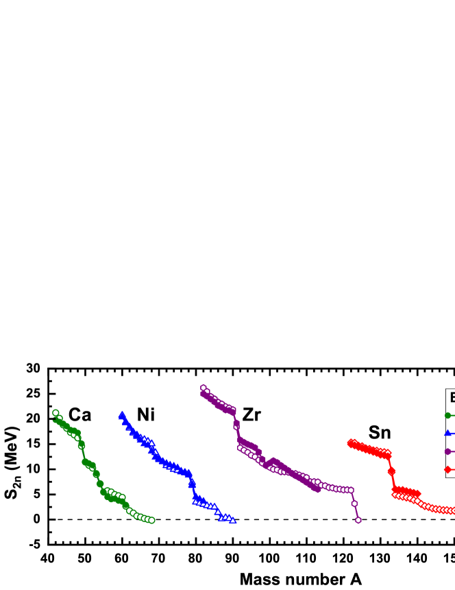
Figure 1: (Color online) Two-neutron separation energies $S_{\rm 2n}$ in the Ca, Ni, Zr, and Sn isotopes as a function of the mass number $A$. Open symbols represent the results calculated by the continuum Skyrme HFB theory with the SLy4 parameter set while the solid ones are the experimental data Wang et al. (2021).

III Numerical details

For the Skyrme interaction in the $ph$ channel, the SLy4 parameter set Chabanat et al. (1998) is adopted. For the pairing interaction in the $pp$ channel, a density dependent $\delta$ interaction (DDDI) is taken,

$$v_{\rm pair}({\bm{r}},{\bm{r}^{\prime}})=\frac{1}{2}(1-P_{\sigma})V_{0}\left[1-\eta\left(\frac{\rho({\bm{r}})}{\rho_{0}}\right)^{\alpha}\right]\delta({\bm{r}}-{\bm{r}^{\prime}}),$$ (16)

with which the pair Hamiltonian $\tilde{h}({\bm{r}}\sigma,{\bm{r}}^{\prime}\sigma^{\prime})$ is reduced to a local pair potential Dobaczewski et al. (1984),

$$\Delta({\bm{r}})=\frac{1}{2}V_{0}\left[1-\eta\left(\frac{\rho({\bm{r}})}{\rho_{0}}\right)^{\alpha}\right]\tilde{\rho}({\bm{r}}),$$ (17)

where the strength of the pairing force $V_{0}=-458.4$ MeV$\cdot$fm³, the density $\rho_{0}=0.08$ fm^-3, and other parameters $\eta=0.71$, $\alpha=0.59$, which are constrained by reproducing the experimental neutron pairing gaps for the Sn isotopes Matsuo (2006); Matsuo et al. (2007); Matsuo and Serizawa (2010). Besides, with these parameters, DDDI can reproduce the scattering length $a=-18.5$ fm in the ${}^{1}S$ channel of the bare nuclear force in the low density limit Matsuo (2006). The cut-off of the quasiparticle states are taken with maximal angular momentum $j_{\rm max}=25/2$ and the maximal quasiparticle energy $E_{\rm cut}=60$ MeV.

The HFB equation is solved in the coordinate space with the space size $R_{\rm box}=20$ fm and mesh size $dr=0.1$ fm. To calculate the densities with the Green’s function, the integrals of the Green’s functions are performed along a contour path $C_{E<0}$, which is chosen as a rectangle with the height $\gamma=0.1$ MeV and the length $E_{\rm cut}=60$ MeV to enclose all the quasiparticle states with negative energies. For the odd-$A$ nuclei, two more contour paths $C_{\rm b}^{+}$ and $C_{\rm b}^{-}$, which only enclose the blocked quasiparticle states at energies $E_{i_{\rm b}}$ and $-E_{i_{\rm b}}$, are introduced due to the blocking effect of the odd unpaired nucleon. For these details, it can be referred to Ref. Sun et al. (2019a). To do the contour integration, an energy step of $\Delta E=0.01$ MeV on the contour path is adopted.

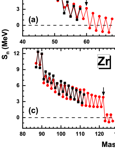
Figure 2: (Color online) Single-neutron separation energies $S_{\rm n}$ as a function of the mass number $A$ in the (a) Ca, (b) Ni, (c) Zr, and (d) Sn isotopes calculated by the continuum Skyrme-HFB theory with the SLy4 parameter set (red circles), in comparison with the experimental data Wang et al. (2021) (black squares).

IV RESULTS AND DISCUSSION

In Fig. 1, the two-neutron separation energies $S_{\rm 2n}(N,Z)=E(N-2,Z)-E(N,Z)$ are plotted for the even-even and odd-even Ca, Ni, Zr, and Sn isotopes. Open symbols are those calculated by the continuum Skyrme-HFB theory with the SLy4 parameter set, in comparison with the available experimental data Wang et al. (2021) denoted by the solid symbols. Good agreements with the experimental data could be observed, indicating the reliability of the continuum Skyrme-HFB theory in the prediction of the neutron drip line. The traditional shell closures, i.e., $N=28$ in the Ca isotopes, $N=50$ in the Ni isotopes, $N=50,82$ in the Zr isotopes, and $N=82$ in the Sn isotopes, could also be observed, where the $S_{\rm 2n}$ drops sharply. For example, in the Sn chain, $S_{\rm 2n}$ drops from $13.25$ MeV at ¹³²Sn to $4.94$ MeV at ¹³⁴Sn with the neutron number exceeding the magic number $N=82$. In the Ca, Ni, and Zr chains, the two-neutron separation energies quickly reach zero at large mass range, resulting in relative short neutron drip lines, which are ⁶⁷Ca, ⁸⁹Ni, and ¹²³Zr, respectively. On the contrary, in the Sn chain, $S_{\rm 2n}$ keeps less than $1.0$ MeV in a wide mass region after the gap of $N=82$ and finally becomes negative until $A=178$, determining ¹⁷⁷Sn as the neutron drip line nucleus. Those weakly bound nuclei are quite interesting due to possible appearance of neutron halos although it is very hard to reach experimentally. In addition, the exploration of the neutron drip line and the determination of the limit of the nuclear existence are significantly important in nuclear physics. However, various theoretical studies show that the predicated neutron drip line is very model dependent Xia et al. (2018). Moreover, different physical quantities or criteria will also predict very different neutron drip lines.

To explore the neutron drip lines in the Ca, Ni, Zr, and Sn isotopes, in Fig. 2, the single-neutron separation energies $S_{\rm n}(N,Z)=E(N-1,Z)-E(N,Z)$ are also plotted. Results by the continuum Skyrme-HFB theory with the SLy4 parameter set are denoted by red circles, which are consistent very well with the experimental data Wang et al. (2021) denoted by the black squares. Strong odd-even staggering is observed in all isotopes. In general, the $S_{\rm n}$ in the even-even nucleus is around $2\sim 3$ MeV larger than the neighbouring odd-$A$ nuclei, which could be explained by that the unpaired odd neutron contributes no pairing energy. As a result, compared with those in Fig. 1, the neutron drip lines determined by the one-neutron separation energy are greatly shortened. In the Ca, Ni, Zr, and Sn isotopes, the drip line nuclei are ⁶⁰Ca, ⁸⁶Ni, ¹²²Zr, and ¹⁴⁸Sn, respectively, the positions of which are indicated by the black arrows. Outside the neutron drip line determined by $S_{\rm n}$, the bound even-even nuclei behave as the interesting Borromean systems. For example, based on the bound nucleus ⁶⁰Ca, ⁶⁰Ca$+n$ is unbound while ⁶⁰Ca$+n+n$ is bound.

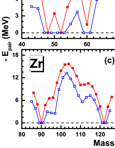
Figure 3: (Color online) Neutron pairing energy $-E_{\rm pair}$ as a function of the mass number $A$ in the (a) Ca, (b) Ni, (c) Zr, and (d) Sn isotopes calculated by the continuum Skyrme-HFB theory with the SLy4 parameter set. The filled and open squares represent the results of the even-even and odd-even nuclei, respectively.

In Fig. 3, we plot the neutron pairing energy $E_{\rm pair}$, which is expressed as,

$$E_{\rm pair}=\frac{1}{2}\int d{\bm{r}}\Delta({\bm{r}})\tilde{\rho}({\bm{r}}).$$ (18)

The red solid symbols are for the even-even nuclei and open symbols for the odd-$A$ nuclei. The neutron pairing energies $E_{\rm pair}$ for the odd-$A$ nuclei are much smaller than those of the neighboring even-even nuclei, due to the absent contribution of pairing energy by the unpaired neutron. This also explains why the drip line determined by the single-neutron separation energy $S_{\rm n}$ is much shorter than that obtained by the two-neutron separation energy $S_{\rm 2n}$. In addition, the pairing energy $E_{\rm pair}$ in each panel behaves as a wave packet as a function of the nuclear mass number, with the wave trough locating at the neutron magic numbers and the crest of wave appearing when the neutron number reaching the half full of the shell. For example, in the Sn isotopes, a large wave package starting from $N=82$ and ending at $N=126$ could be observed, with the highest value at the position of the neutron number $N=102$. As a result, the traditional shell closures, i.e., $N=28,40$ in the Ca isotopes, $N=40,50$ in the Ni isotopes, $N=50,82$ in the Zr isotopes, and $N=82,126$ in the Sn isotopes, could also be obviously observed, which are consistent with those obtained in Fig. 1. In addition, a sub-shell $N=32$ is also observed in the Ca isotopes.

In the following, we will explore the possible neutron halo phenomena in the Ca, Ni, Zr, and Sn isotopes, especially in the weakly bound nuclei near the drip line, in which the neutron Fermi surfaces are very close to the continuum threshold and the valence neutron could be easily scattered to the continuum and occupy the resonant states.

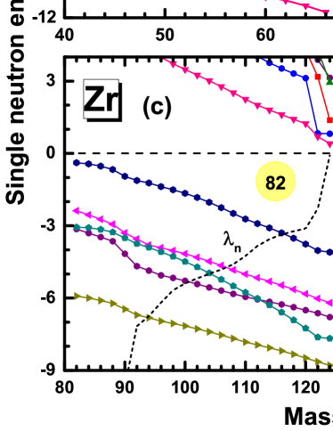
Figure 4: (Color online) Canonical single-particle levels for neutrons around the fermi surface in the (a) Ca, (b) Ni, (c) Zr, and (d) Sn isotopes calculated by the continuum Skyrme-HFB theory. The short dashed lines represent the Fermi surface.

In Fig. 4, the neutron canonical single-particle structure as functions of the mass number are plotted for the (a) Ca, (b) Ni, (c) Zr, and (d) Sn isotopes. For the details how to get the canonical single-particle levels, it can be referred to Refs. Qu and Zhang (2019b); Qu et al. (2022). The neutron Fermi energy $\lambda_{\rm n}$ as well as the canonical single-particle energies $\varepsilon$ are shown. With the neutron number increasing, the Fermi energy $\lambda_{\rm n}$ in each chain is raised up and finally reaches the continuum threshold while all the HF single-particle levels fall down. The traditional shell closures, i.e., $N=28,40$ in the Ca isotopes, $N=40,50$ in the Ni isotopes, $N=82$ in the Zr isotopes, and $N=82$ in the Sn isotopes, could be observed, where the big gaps could be observed obviously. Different single-particle structures are revealed in the Ca, Ni, Zr, and Sn chains, based on which halos could be formed easily or hardly. In the Ni chain, above the shell closure of $N=50$, there are several weakly bound states and the low-lying resonant sates with small angular momenta, i.e., $2d_{5/2}$, $3s_{1/2}$, and $2d_{3/2}$, which create good opportunities for the formation of halos. For the Sn chain, which is quite similar to the Ni chain but has more advantages for halo formation, more weakly bound states and the low-lying resonant sates exist above the $N=82$ shell closure. Besides, the Fermi surface $\lambda_{\rm n}$ approaches zero gradually and the Sn isotopes in a large mass reagin are weakly bound. In the Ca chain, above the shell closure of $N=40$, there is mainly the 1$g_{9/2}$ state, which evolves from a single-particle resonant state ($A\leq 62$) to a weakly bound level ($A\geq 64$). Although there is a visitable possibility for valence neutrons occupy 1$g_{9/2}$ orbital, the contributed density is very localized due to the big central barrier. In the neutron-rich Ca isotopes, the low-lying resonant states $3s_{1/2}$ and $2d_{5/2}$ also play important roles. The worst case happens in the Zr chain where the shell closure of $N=82$ locates around the threshold of continuum and it’s hard for the valence neutrons to overcome the big gap and occupy the continuum. Thus, halos are not easy to be formed in the Zr isotopes.

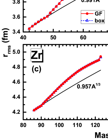
Figure 5: (Color online) Neutron root-mean-square (rms) radii $r_{\rm rms}$ for the (a) Ca, (b) Ni, (c) Zr, and (d) Sn isotopes calculated by the Skyrme-HFB theory with the Green’s function method (filled circles and solid lines), in comparison with the results by the discretized method (open triangles and dashed lines).

In Fig. 5, the neutron root-mean-square (rms) radii,

$$r_{\rm rms}=\sqrt{\frac{\int dr4\pi r^{4}\rho(r)}{\int dr4\pi r^{2}\rho(r)}},$$ (19)

are plotted in the Ca, Ni, Zr, and Sn isotopes, which are obtained by the Skyrme-HFB calculations both with the Green’s function method (filled circles and solid lines) and box-discretized method (open triangles and dashed lines) employing the SLy4 parameter set, in comparison with the radii $r=b_{0}A^{1/3}$ in the traditional liquid-drop model (black lines), where the coefficient $b_{0}$ could be determined by the radii of deeply bound nuclei. In the Ca, Ni, Zr, and Sn chains, they are $r\thickapprox 0.991A^{1/3}$, $0.984A^{1/3}$, $0.957A^{1/3}$, and $0.961A^{1/3}$, respectively decided by the rms radii of stable nuclei with neutron number less than the shell closure $N=28,50,50$ and $80$. In each chain, by adding more neutrons, the nuclear rms radii $r_{\rm rms}$ increase steeply and veer off the radii $A^{1/3}$ rule. For example, in the Ca chain, compared with the isotopic trend in $N\leqslant 20$, which gives an extrapolation as $r\thickapprox 0.991A^{1/3}$, the neutron rms radii in ⁵⁰Ca and the heavier isotopes display steep increases with $N$. In those mass area, possible neutron halos may occur. Besides, obvious odd-even staggering of rms radii could be observed in the Sn chain, where the odd-$A$ nuclei ^151-165Sn own larger rms radii than the neighbouring two even-even nuclei. The detailed explanations could be seen in Ref. Sun et al. (2019a). The odd-even staggering phenomena in nuclear radii and nuclear mass have attracted great interests in the past years and lots of efforts have been done, such as the works in Refs. Satuła et al. (1998); Dobaczewski et al. (2001); Litvinov et al. (2005); Hagino and Sagawa (2012); Wang et al. (2013); Coraggio et al. (2013); Chen et al. (2015).

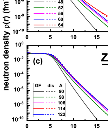
Figure 6: (Color online) Neutron density $\rho(r)$ for the (a) Ca, (b) Ni, (c) Zr, and (d) Sn isotopes calculated by the Skyrme-HFB theory with the Green’s function method (solid lines), in comparison with the results by the discretized method (dashed lines).

In the exotic nuclei, extended density distributions in the coordinate space is often behaved. Thus, in Fig. 6, to explore the exotic structures in the (a) Ca, (b) Ni, (c) Zr, and (d) Sn isotopes, we also plotted the neutron density distributions $\rho(r)$, where the solid lines are those obtained by the Green’s function method in comparison with the results by the box-discretized method denoted by the dashed lines. It is a global trend that the neutron density distributions are extended further with the increasing neutron number. The shell structures influence the density distribution significantly, i.e., compared with the bound nuclei, the density distributions of the neutron-rich nuclei in the (a) Ca, (b) Ni, (c) Zr, and (d) Sn isotopes with the neutron number exceeding the neutron closure $N=28,50,50,82$ are much more extended, which is consistent with the behaviors of the rms radii plotted in Fig. 5. In further, compared with the Ca and Zr chains, the Ni and Sn chains perform the more dispersion distributions in the densities, which can be explained by their small two-neutron separation energies $S_{\rm 2n}$ in a large mass range plotted in Fig. 1 indicating them the very weakly bound systems. In the case of the Zr isotopes, the density distributions in the total chain are relatively localized, and in combination with the large $S_{\rm 2n}$ plotted in Fig. 1, we are inclined to believe the absence of the halos in Zr isotopes. However, taking the RCHB theory with the NLSH parameter set Meng and Ring (1998b) and the continuum Skyrme-HFB theory with the SKI4 parameter set Grasso et al. (2006); Zhang et al. (2012), giant halos have been predicated. In all the isotopes, compared with the box-discretized method which gives nonphysical sharp decreases of the density distributions at the space boundary, Green’s function method can describe well the extended density distributions, especially for the very neutron-rich isotopes. Besides, the densities obtained by the Green’s function method can be independent on the space sizes as discussed in Ref. Sun et al. (2019a), which is determined basically by the proper boundary conditions of the bound states, weakly bound sates and the continuum employed when constructing the Green’s functions.

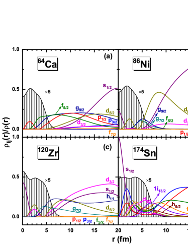
Figure 7: (Color online) Contributions of different partial waves to the total neutron density, $\rho_{lj}(r)/\rho(r)$, as a function of the radial coordinate $r$ for the neutron-rich nuclei (a) ⁶⁴Ca, (b) ⁸⁶Ni, (c) ¹²⁰Zr, and (d) ¹⁷⁴Sn. The shallow regions are for the nuclear density distributions $\rho(r)$, which are rescaled by multiplying a factor of $5$.

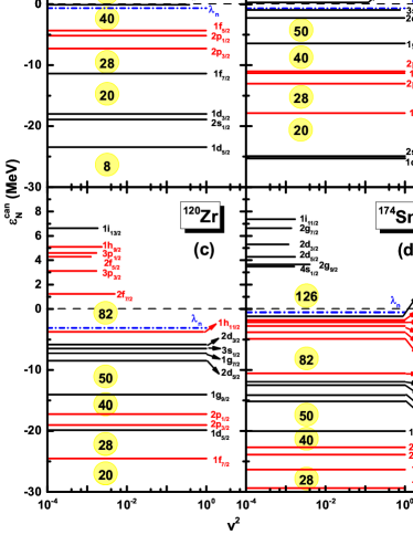
Figure 8: (Color online) Neutron canonical single-particle levels in the (a) ⁶⁴Ca, (b) ⁸⁶Ni, (c) ¹²⁰Zr, and (d) ¹⁷⁴Sn calculated by the Skyrme-HFB theory with the Green’s function method. The blue dashed lines represent the Fermi surface. The occupation probabilities $v^{2}$ for the canonical orbitals are proportional to the lengths of the lines (in logarithmic scale).

To explore the contributions of different partial waves on the extended density distributions in Fig. 6, taking the neutron-rich (a) ⁶⁴Ca, (b) ⁸⁶Ni, (c) ¹²⁰Zr, and (d) ¹⁷⁴Sn as examples, we plot in Fig. 7 the compositions $\rho_{lj}(r)/\rho(r)$ as functions of the radial coordinate $r$ and show in Fig. 8 the neutron canonical single-particle levels as well as the occupation probabilities. It can be clearly seen that outside the nuclear surface referring to the right boundary of the shallow regions for the total nuclear density distributions, it’s the orbitals locating around the Fermi surface that play the main role of the density distributions. For example, in the neutron-rich ⁶⁴Ca, the partial waves $p_{1/2}$, $f_{5/2}$, $g_{9/2}$, $s_{1/2}$, and $d_{5/2}$ contribute a lot for the total density in the area of $5~{}{\rm fm}<r<15~{}{\rm fm}$. Those levels are located around within $5~{}$MeV above and below the Fermi surface as shown in Fig. 8. When going further in the coordinate space with $r>15~{}$fm, the contributions of the partial waves $s_{1/2}$ and $d_{5/2}$ with low angular momenta increase obviously while others reduce their contributions. In the case of ⁸⁶Ni, the single-particle levels $2d_{5/2}$, $3s_{1/2}$, and $2d_{3/2}$, which are located above the neutron shell of $N=50$ and close to the Fermi surface, play the main role of the neutron density distribution. Although the single-particle resonant state $1g_{7/2}$ in the continuum is also very close to the Fermi surface, very small contribution for the density in large coordinate space is observed due to the effect of the large centrifugal barrier. For the nucleus ¹²⁰Zr with the neutron number very close to the closure of $N=82$, the single-particle levels between the closures $N=50$ and $N=82$ including $2d_{5/2}$, $1g_{7/2}$, $3s_{1/2}$, $2d_{3/2}$, and $1h_{11/2}$, contribute a lot for the densities in large coordinate space. The very small occupation of the single-particle resonant state $2f_{7/2}$ leads to little contribution to the density. Regarding to the neutron-rich ¹⁷⁴Sn with the neutron number exceeding the closure of $N=82$, the weakly bound single-particle levels $2f_{7/2}$, $2f_{5/2}$, $3p_{3/2}$, and $3p_{1/2}$ with small angular momentum play the key role for the extended density distributions in the large coordinate space. According to those analysis, we can conclude that it is the single-particle levels around the Fermi surface especially the waves with low angular momenta that cause the extended nuclear density.

In Fig. 8, the particle occupation probabilities $v^{2}$ on different canonical levels $\varepsilon_{\rm N}^{\rm can}$ are presented and denoted by the length of the lines. Without pairing, the values of the occupation probabilities $v^{2}$ should be either one or zero with the boundary line of the Fermi surface. With the effect of pairing, the nucleons occupied the levels below the Fermi surface can be scattered to higher levels and result in the occupations of the weakly bound states above the Fermi surface and even levels in the continuum. In the neutron-rich nuclei ⁶⁴Ca, ⁸⁶Ni, ¹²⁰Zr, and ¹⁷⁴Sn, the number of neutrons ${\displaystyle N_{\lambda}=\sum_{\varepsilon_{k}>\lambda_{\rm n}}(2j+1)v_{k}^{2}}$ scattered above the Fermi surface $\lambda_{\rm n}$ are $4.33$, $2.51$, $0.159$, and $0.173$, respectively. In the case of ⁶⁴Ca, the very weakly bound single-particle $1g_{9/2}$ contribute around $3.7$ neutrons.

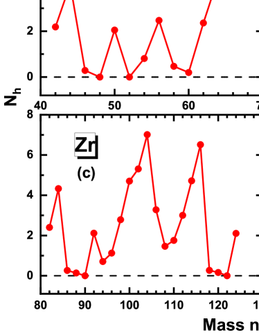
Figure 9: (Color online) Number of the neutrons $N_{\lambda}$ occupied the single-particle levels above the Fermi surface $\lambda_{n}$ as a function of the mass number $A$ for the (a) Ca, (b) Ni, (c) Zr, and (d) Sn isotopes calculated by the Skyrme-HFB theory with the Green’s function method.

To explore the effects of pairing, we plot in Fig. 9 the number of neutrons $N_{\lambda}$ scattered above the Fermi surface for the (a) Ca, (b) Ni, (c) Zr, and (d) Sn chains obtained by the Skyrme-HFB theory with the Green’s function method. It can be seen clearly that substantial neutrons have been scattered from the single-particle levels below the Fermi surface to the weakly bound states above the Fermi surface and even levels in the continuum due to the pairing, especially in the nuclei with the neutron number filling the half-full shells. Besides, very obvious shell structure could be observed. With the number of neutrons reaching a magic number, i.e., $N=28,40$ in the Ca isotopes, $N=40,50$ in the Ni isotopes, $N=50,82$ in the Zr isotopes, and $N=82,126$ in the Sn isotopes, $N_{\lambda}$ is almost zero due to the absence of the pairing for the closed-shell nuclei. Besides, at the points of $N=32$ in the Ca isotopes, $N=54,68$ in the Zr isotopes, and $N=88$ in the Sn isotopes, very small numbers of neutron $N_{\lambda}$ are obtained, which indicate weak pairing in those nuclei. On the other hand, it can also predict the possible existence of sub-shells and new magic numbers. Furthermore, the evolution of $N_{\lambda}$ is basically consistent with the trend of pair energy $-E_{\rm pair}$ in Fig. 3.

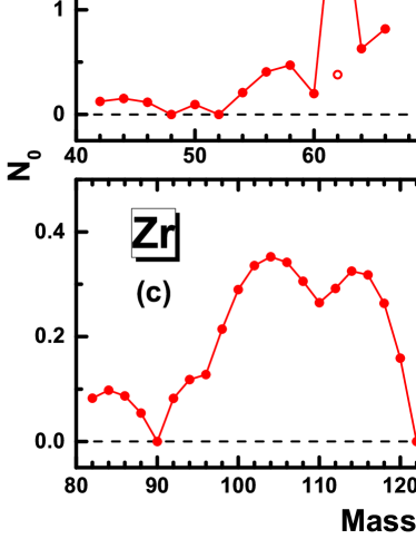
Figure 10: (Color online) Number of neutrons $N_{0}$ occupied in the continuum (above the threshold $\varepsilon=0$ MeV) as a function of the mass number $A$ for the (a) Ca, (b) Ni, (c) Zr, and (d) Sn isotopes calculated by the Skyrme-HFB theory with the Green’s function method.

In Fig. 10, we further investigate the number of neutrons occupied in the continuum with the single-particle energies $\varepsilon>0$ MeV, i.e., ${\displaystyle N_{0}=\sum_{\varepsilon_{k}>0}(2j+1)v_{k}^{2}}$. Compared with the number of neutron $N_{\lambda}$ occupied in the levels above the Fermi surface, the number of neutrons occupied in the continuum $N_{0}$ is reduced drastically. For example, in the Ca chain, $N_{0}$ is less than one in all isotopes except ⁶²Ca. In ⁶²Ca, the single-particle level $1g_{g/2}$ displays as a low-lying resonant state with energy of $\varepsilon=0.198$ MeV and a high occupation probability of $v^{2}=0.197$, resulting to almost $1.979$ neutrons occupying on it. But in the neighboring ⁶⁰Ca, very small occupation probability $v^{2}=0.015$ of $1g_{9/2}$ is obtained while in ⁶⁴Ca, the $1g_{9/2}$ state drops to be a weakly bound level with the energy of $\varepsilon=-0.072$ MeV. After removing the neutron contribution from $1g_{g/2}$ in ⁶²Ca, only $0.38$ neutrons are in the continuum, which is denoted by an empty circle in panel (a). Except the Sn chain, the shape of $N_{0}$ is very close to those of pairing energy and pairing gap. Although the case of Sn chain becomes very complex, we can still observe the shell structure at $N=82$ and $N=126$ where $N_{0}$ is almost zero.

V SUMMARY

In this work, the exotic nuclear properties of neutron-rich Ca, Ni, Zr, and Sn isotopes are studied systematically taking the continuum Skyrme-HFB theory in the coordinate space formulated with the Green’s function method, in which the pairing correlations, the couplings with the continuum, and the blocking effects for the unpaired nucleon in odd-$A$ nuclei are treated properly.

Firstly, both the two-neutron separation energies $S_{\rm 2n}$ and one-neutron separation energies $S_{\rm n}$ are calculated, which consist well with the experimental data. Great differences exist for the drip lines determined by $S_{\rm 2n}$ and $S_{\rm n}$, and in the Ca, Ni, Zr, and Sn isotopes, the determined drip line nuclei are ⁶⁷Ca, ⁸⁹Ni, ¹²³Zr, and ¹⁷⁷Sn judging by $S_{\rm 2n}$ while they are ⁶⁰Ca, ⁸⁶Ni, ¹²²Zr, and ¹⁴⁸Sn according to $S_{\rm n}$. For further research, the pairing energies for even-even and odd-even nuclei are studied. We found that the neutron pairing energies $-E_{\rm pair}$ of the odd-$A$ nuclei are around $2$ MeV smaller in comparison with those of the neighboring even-even nuclei, which can be explained by the absent contribution of pairing energy by the single unpaired odd neutron. This also explains why the drip lines determined by $S_{\rm n}$ are much shorter than those by $S_{\rm 2n}$. In addition, from the fluctuation trends of the pairing energy, the traditional neutron magic numbers are clearly displayed, i.e., $N=28,40$ in the Ca isotopes, $N=40,50$ in the Ni isotopes, $N=50,82$ in the Zr isotopes, and $N=82,126$ in the Sn isotopes.

Secondly, to explore the possible halo structures in the neutron-rich Ca, Ni, Zr, and Sn isotopes, the neutron single-particle structures, the root-mean-square radii, and the density distributions are investigated. In the neutron-rich Ca, Ni, Sn nuclei, especially the weakly bound nuclei close to neutron drip line, the rms radii have sharp increases with significant deviations from the traditional $r\varpropto A^{1/3}$ rule. Besides, very diffuse spatial density distributions are also observed in those nuclei, which reflects the possible halo phenomenon therein. By analyzing the contribution of different partial waves to the total density, we found that it is the orbitals locating around the Fermi surface especially the waves with low angular momenta that cause the extended nuclear density and large rms radii.

Finally, the number of halo nucleons which could reflects the effects of pairing are discussed. Two different types of the number of the neutrons are defined, i.e., $N_{\lambda}$ occupied the single-particle levels above the Fermi surface $\lambda_{n}$ and $N_{0}$ occupied in the continuum. We found that the evolutions of $N_{\lambda}$ and $N_{0}$ with the mass number $A$ are basically consistent with the trend of pairing energy $-E_{\rm pair}$, which supports the key role of the pairing correlations in the halo phenomena.