Skill Machines: Temporal Logic Composition in Reinforcement Learning

Abstract

A major challenge in reinforcement learning is specifying tasks in a manner that is both interpretable and verifiable. One common approach is to specify tasks through reward machines—finite state machines that encode the task to be solved. We introduce skill machines, a representation that can be learned directly from these reward machines that encode the solution to such tasks. We propose a framework where an agent first learns a set of base skills in a reward-free setting, and then combines these skills with the learned skill machine to produce composite behaviours specified by any regular language, such as linear temporal logics. This provides the agent with the ability to map from complex logical task specifications to near-optimal behaviours zero-shot. We demonstrate our approach in both a tabular and high-dimensional video game environment, where an agent is faced with several of these complex, long-horizon tasks. Our results indicate that the agent is capable of satisfying extremely complex task specifications, producing near optimal performance with no further learning. Finally, we demonstrate that the performance of skill machines can be improved with regular offline reinforcement learning algorithms when optimal behaviours are desired.

1 Introduction

Reinforcement learning (RL) is a promising framework for developing truly general agents capable of acting autonomously in the real world. Despite recent successes in the field, ranging from video games [4] to robotics [16], there are several shortcomings to existing approaches that hinder RL’s real-world applicability. One issue is that of sample efficiency—while it is possible to collect millions of data points in a simulated environment, it is simply not feasible to do so in the real world. This inefficiency is exacerbated if a single agent is required to solve multiple tasks (as we would expect of a generally intelligent agent).Another issue arises when an agent is required to solve a long horizon task in the presence of a sparse learning signal. In this case, it is often near impossible for the agent to solve the task, regardless of how much data it collects, since the sequence of actions to execute before a learning signal is received is too large [2]. However, this can be mitigated by leveraging higher-order skills, which shortens the planning horizon [26].

A desirable characteristic of generally intelligent agents is their ability to reuse learned behaviours to solve new tasks [27], preferably without further learning. One approach to overcoming this challenge is to rely on composition, where an agent first learns individual skills and then combines them to produce novel behaviours. There are several notions of compositionality in the literature, such as temporal composition, where skills are invoked one after the other [26, 7], and concurrent composition, where skills are combined to produce a new behaviour to be executed [28, 25, 29, 1].

Notably, work by Nangue Tasse et al. [20] has demonstrated how an agent can learn skills that can be combined using Boolean operators, such as negation and conjunction, to produce semantically meaningful behaviours without further learning. An important benefit to this approach to compositionality is that it provides a way to address another key issue with RL: tasks, as defined by reward functions, can be notoriously difficult to specify. This may lead to undesired behaviours that are not easily interpretable and verifiable. Composition that enables human-understandable task specifications and produces reliable behaviours then represents a major step towards safe AI [10].

Unfortunately, these compositions are strictly concurrent and cannot be chained to solve temporally-specified tasks. One solution to this issue is reward machines—finite state machines that encode the tasks to solve [13]. While this obviates the sparse reward problem, the agent is still required to learn how to solve a given task through environment interaction, and the subsequent solution is monolithic, restricting its applicability to new tasks and limiting the reliability of resulting behaviours.

In this work, we combine these two approaches to develop an agent capable of zero-shot concurrent and temporal composition. We particularly focus on temporal logic composition, such as linear temporal logic (LTL) [24], allowing agents to sequentially chain and order their skills while ensuring certain conditions are always or never met. We make the following contributions: (a) we propose skill machines, a finite state machine that can be autonomously learned by a compositional agent, and which can be used to solve any task expressible as a finite state machine without further learning; (b) we prove that these skill machines are satisficing—given a task specification, an agent can successfully solve it while adhering to any constraints; and (c) we demonstrate our approach in several environments, including a high-dimensional video game domain. Having learned a set of base skills in a reward-free setting, our results indicate that our method is capable of producing near-optimal behaviour for a variety of long-horizon tasks without further learning.

2 Background

We model the agent’s interaction with the world as a Markov Decision Process (MDP), given by $(\mathcal{\mathcal{S}},\mathcal{A},P,R,\gamma)$, where (i) $\mathcal{S}\subseteq\mathbb{R}^{n}$is the $n$-dimensional state space; (ii) $\mathcal{A}$is the set of (possibly continuous) actions available to the agent; (iii) $P(s^{\prime}|s,a)$is the dynamics of the world, representing the probability of the agent reaching state $s^{\prime}$ after executing action $a$ in state $s$; (iv) $R$is a reward function bounded by $[R_{\text{MIN}},R_{\text{MAX}}]$ that represents the task the agent needs to solve; and (v) $\gamma\in[0,1]$is a discount factor.

The aim of the agent is to compute a Markov policy $\pi$ from $\mathcal{S}$ to $\mathcal{A}$ that optimally solves a given task. Instead of directly learning a policy, an agent will often instead learn a value function that represents the expected return following policy $\pi$ from state $s$: $V^{\pi}(s)=\mathbb{E}^{\pi}\left[\sum_{t=0}^{\infty}\gamma^{t}R(s_{t},a_{t},s_{t+1})\right]$. A more useful form of value function is the action-value function $Q^{\pi}(s,a)$, which represents the expected return obtained by executing $a$ from $s$, and then following $\pi$. The optimal action-value function is given by $Q^{*}(s,a)=\max_{\pi}Q^{\pi}(s,a)$ for all states $s$ and actions $a$, and the optimal policy follows by acting greedily with respect to $Q^{*}$ at each state.

2.1 Logical Composition in the Multitask Setting

We are interested in the multitask setting, where an agent is required to reach a set of goals in some goal space $\mathcal{G}\in\mathcal{S}$. We assume that all tasks share the same state space, action space and dynamics, but differ in their reward functions. We model this setting by defining a background MDP $M_{0}=\langle\mathcal{\mathcal{S}}_{0},\mathcal{A}_{0},P_{0},R_{0}\rangle$ with its own state space, action space, transition dynamics and background reward function. Any individual task $\tau$ is then specified by a task-specific reward function $R_{\tau}$ that is non-zero only for transitions entering a state in $\mathcal{G}$. The reward function for the resulting MDP is then simply $R_{0}+R_{\tau}$.

Nangue Tasse et al. [20] consider the case where $R_{\tau}\in\{R_{\text{MIN}},R_{\text{MAX}}\}$ and develop a framework that allows agents to apply Boolean operations—conjunction ($\wedge$), disjunction ($\vee$) and negation ($\neg$)—over the space of tasks and value functions. This is achieved by first defining the goal-oriented reward function $\bar{R}$ which extends the task rewards $r$ to penalise an agent for achieving goals different from the one it wished to achieve:

$$\bar{R}(s,g,a,s^{\prime})\coloneqq\begin{cases}\bar{R}_{\text{MIN}}&\text{if }g\neq s\text{ and }s^{\prime}\text{ is absorbing }\\ R(s,a)&\text{otherwise},\end{cases}$$ (1)

where $\bar{R}_{\text{MIN}}$ is a large negative penalty that can be derived from the bounds of the reward function.

Using Equation 1, we can define the related goal-oriented value function as:

$$\bar{Q}(s,g,a)=\bar{R}(s,g,a)+\gamma\int_{\mathcal{S}}\bar{V}^{\bar{\pi}}(s^{\prime},g)P_{(s,a)}(ds^{\prime}),$$ (2)

where $\bar{V}^{\bar{\pi}}(s,g)=\mathbb{E}_{\bar{\pi}}\left[\sum_{t=0}^{\infty}\gamma^{t}\bar{R}(s_{t},g,a_{t},s_{t+1})\right]$.

If a new task can be represented as the logical expression of previously learned tasks, Nangue Tasse et al. [20] prove that the optimal policy can immediately be obtained by composing the learned goal-oriented value functions using the same expression. For example, the union ($\vee$), intersection ($\wedge$), and negation ($\neg$) of two goal-reaching tasks $A$ and $B$ can be solved as follows (we omit the value functions’ parameters for readability):

$$\bar{Q}^{*}_{A\vee B}=\bar{Q}^{*}_{A}\vee\bar{Q}^{*}_{B}\coloneqq\max\{\bar{Q}^{*}_{A},\bar{Q}^{*}_{B}\}$$

$$\bar{Q}^{*}_{A\wedge B}=\bar{Q}^{*}_{A}\wedge\bar{Q}^{*}_{B}\coloneqq\min\{\bar{Q}^{*}_{A},\bar{Q}^{*}_{B}\}$$

$$\bar{Q}^{*}_{\neg A}=\neg\bar{Q}^{*}_{A}\coloneqq\left(\bar{Q}^{*}_{SUP}+\bar{Q}^{*}_{INF}\right)-\bar{Q}^{*}_{A},$$

where $\bar{Q}^{*}_{SUP}$ and $\bar{Q}^{*}_{INF}$ are the goal-oriented value functions for the maximum task ($r=R_{\text{MAX}}$ for all $\mathcal{G}$) and minimum task ($r=R_{\text{MIN}}$ for all $\mathcal{G}$) , respectively . Following Nangue Tasse et al. [21], we refer to these goal-oriented value functions as world value functions (WVFs).

2.2 Reward Machines

One difficulty with the standard MDP formulation is that the agent is often required to solve a complex long-horizon task using only a scalar reward signal as feedback from which to learn. To overcome this, Icarte et al. [13] propose reward machines (RMs), which provide structured feedback to the agent in the form of a finite state machine. RMs encode a reward function using a set of propositional symbols $\mathcal{P}$ that represent abstract environment features as follows:

Definition 1 (Reward Machine).

Given a set of propositional symbols $\mathcal{P}$, states $\mathcal{S}$ and actions $\mathcal{A}$, a reward machine is a tuple $R_{\mathcal{P}\mathcal{S}\mathcal{A}}=\langle U,u_{0},F,\delta_{u},\delta_{r}\rangle$ where (i) $U$ is a finite set of states; (ii) $u_{0}\in U$ is an initial state; (iii) $F$ is a finite set of terminal states; (iv) $\delta_{u}:U\times 2^{\mathcal{P}}\to U\cup F$ is the state-transition function; and (v) $\delta_{r}:U\to[\mathcal{S}\times\mathcal{A}\times\mathcal{S}\to\mathbb{R}]$ is the state-reward function.

RMs consist of a finite set of states $U$, each of which represents a set of propositions that are true at the given environment state. Transitions between RM states are governed by $\delta_{u}$, and the RM emits a reward function according to $\delta_{r}$. A particular instantiation of an RM that is used in practice is a simple reward machine (SRM), which restricts the form of the state-reward function to be $\delta_{r}:U\times 2^{\mathcal{P}}\to\mathcal{R}$ [13]. In other words, when a transition between $u,u^{\prime}\in U$ is made, the SRM emits a single scalar instead of a function (as in the case of RMs).

To incorporate RMs into the RL framework, the agent must be able to determine which abstract propositions are true at any given state. To achieve this, the agent is equipped with a labelling function $L:\mathcal{S}\times\mathcal{A}\times\mathcal{S}\to 2^{\mathcal{P}}$ that assigns truth values to the propositions based on the agent’s interaction with its environment. The agent can then learn a policy in a new decision process where the reward function in the original MDP is replaced with the RM, which is defined by the tuple $\langle\mathcal{S},\mathcal{A},P,\gamma,\mathcal{P},L,U,u_{0},F,\delta_{u},\delta_{r}\rangle$. The agent’s aim is now to learn a policy over the joint MDP and RM state space $\pi:\mathcal{S}\times U\to\mathcal{A}$, which can be achieved with standard algorithms such as $Q$-learning [13].

3 Leveraging Skill Composition for Temporal Logic Tasks

To describe our approach to temporal composition, we use the Office Gridworld [13] as a running example. In the environment, illustrated by Figure 1(a), an agent (blue square) can move to adjacent cells in any of the cardinal directions. It can also pick up coffee or mail at locations $\scaleobj{1}{\scalerel*{\includegraphics{emoji/coffee}}{\textrm{\copyright}}}$ or $\scaleobj{1}{\scalerel*{\includegraphics{emoji/mail}}{\textrm{\copyright}}}$ respectively, and it can deliver them to the office at location $o$. Cells marked $\coAsterisk$ indicate decorations that are broken if the agent collides with them, and cells marked $A$–$D$ indicate the centres of the corner rooms. Hence, the reward machines that specify tasks in this environment are defined over 8 propositions: $\mathcal{P}=\{\scaleobj{1}{\scalerel*{\includegraphics{emoji/coffee}}{\textrm{\copyright}}},\scaleobj{1}{\scalerel*{\includegraphics{emoji/mail}}{\textrm{\copyright}}},\coAsterisk,o,A,B,C,D\}$, where propositions are true when the agent is at their respective locations.

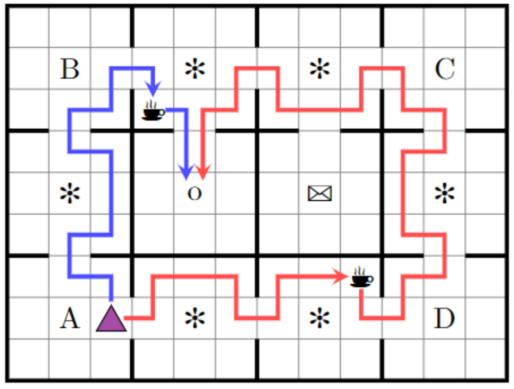
(a) Office Gridworld [13]

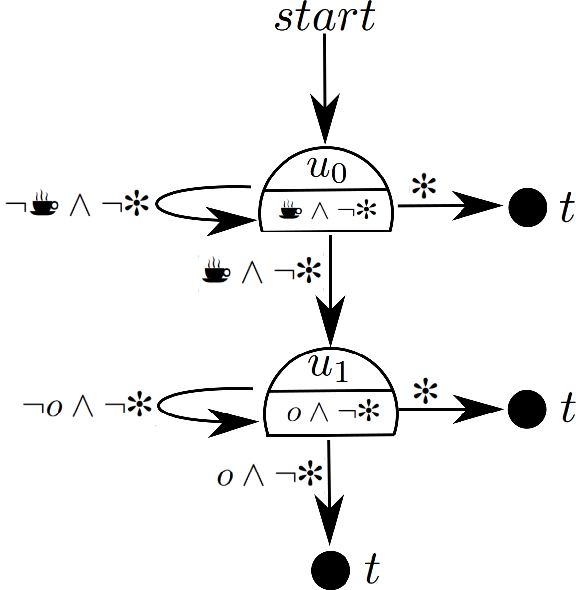
(b) Task 1 skill machine

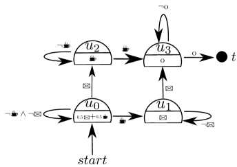
(c) Task 2 skill machine

Figure 1: Illustration of the office gridworld, and the skill machines for tasks (b) “deliver coffee to the office without breaking any decoration”, and (c) “deliver coffee and mail to the office.”

3.1 Task Space

We now define the set of tasks to be considered. We first introduce the concept of constraints $C\subseteq\mathcal{P}$, which are the set of propositions that an agent should avoid setting to true and corresponds to the global operator $G$ in a linear temporal logic (LTL) specification. An example of a constraint might be that the agent should complete a task, but avoid breaking any decorations while doing so. We can now define the notion of base tasks, which will later be composed.

Definition 2 (Task Primitive).

Let $M=\langle\mathcal{\mathcal{S}}_{0},\mathcal{A}_{0},P_{0},R_{0}\rangle$ be a background MDP. We define a set of task primitives in this domain as $\mathcal{M}_{\mathcal{G}}=\{\langle\mathcal{S},\mathcal{A},P,R,\gamma\rangle\}$ with absorbing goal space $\mathcal{G}=2^{\mathcal{P}}$ and labelling function $L$, where

$$\mathcal{S} \coloneqq(\mathcal{S}_{0}\times 2^{C})\cup 2^{\mathcal{P}},\textrm{where $C$ is the set of constraints};$$

$$\mathcal{A} \coloneqq\mathcal{A}_{0}\times\mathcal{A}_{\tau},\textrm{ where }\mathcal{A}_{\tau}=\{0,1\}\textrm{ represents whether or not to terminate a task};$$

$$P(\langle s_{0},c\rangle,\langle a_{0},a_{\tau}\rangle) \coloneqq\begin{cases}L(s_{0},a_{0},s^{\prime}_{0})&\text{if }a_{\tau}=1\\ \langle s^{\prime}_{0},c^{\prime}\rangle&\text{otherwise}\end{cases},$$

$$\textrm{ where }s^{\prime}_{0}\sim P_{0}(\cdot|s_{0},a_{0})\textrm{ and }c^{\prime}=c\cup(c\cap L(s_{0},a_{0},s^{\prime}_{0}));$$

$$R(\langle s_{0},c\rangle,\langle a_{0},a_{\tau}\rangle) \coloneqq\begin{cases}R_{\tau}\in\{R_{\text{MIN}},R_{\text{MAX}}\}&\text{if }a_{\tau}=1\\ R_{0}(s_{0},a_{0})&\text{otherwise}.\end{cases}$$

The above defines the tasks’ state space to be the product of the environment state and the set of constraints, incorporating the set of propositions that are currently true. The action space is augmented with a terminating action following Barreto et al. [7] and Nangue Tasse et al. [20], which indicates that the agent wishes to achieve the goal it is currently at, and is similar to an option’s termination condition [26]. The transition dynamics update the environment state and constraints set to true when a regular action is taken, and use the labelling function to return the set of propositions achieved when the agent decides to terminate. Finally, the agent receives the regular environment reward when taking an action, but a task-specific goal reward when it terminates. We will assume that the environment and task-specific rewards are such that the optimal policies for all tasks are guaranteed to reach desired reachable goal states—a common example is to have a reward of $1$ at desired goal states and no rewards everywhere else.

Equipped with this definition, we can now define the set of all tasks under consideration:

Definition 3 (Task space).

The set of all tasks $\mathcal{M}$ is all linear preferences over task primitives:

$$\mathcal{M}=\Big{\{}\langle\mathcal{S},\mathcal{A},P,R_{\mathbf{w}},\gamma\rangle:R_{\mathbf{w}}(s,a)=\sum\limits_{i=1}^{|\mathcal{M}_{\mathcal{G}}|}w_{i}R_{i}(s,a)\text{ and }\mathbf{w}\in\mathbb{R}^{|\mathcal{M}_{\mathcal{G}}|}\Big{\}}$$ (3)

This definition of task space gives us a very general notion of task that is still grounded in achieving goals. It also subsumes most definitions of tasks considered in the composition literature, including Boolean algebra tasks from Nangue Tasse et al. [20] and linear preference tasks from Barreto et al. [8]. Hence, we will restrict our attention to reward machines whose rewards per state originate from the defined task space (instead of arbitrary real-valued functions that are not grounded in achieving goals in an environment). We denote such reward machines as $R_{\mathcal{M}\mathcal{S}\mathcal{A}}=\langle U,u_{0},F,\delta_{u},\delta_{\mathcal{M}}\rangle$ where $\delta_{\mathcal{M}}$ maps from RM-states to task rewards.

3.2 Skill machines

The goal space of a primitive task is defined by a set of Boolean propositions. We can leverage prior work to solve each individual task using a set of base primitive skills [20]. We therefore only need concern ourselves with how to solve any task expressed as a linear combination of the primitive tasks. Fortunately, Theorem 1 below demonstrates that a linear combination of base skills does just this.

Theorem 1.

Let $\mathbf{R}_{\mathcal{M}_{\mathcal{G}}}$ be a vector of rewards for each primitive task, and $\mathbf{\bar{Q}}^{*}_{\mathcal{G}}$ be the corresponding vector of optimal WVFs. Then, for a task $m\in\mathcal{M}$ with reward function $R_{\mathbf{w}}=\mathbf{w}\cdot\mathbf{R}_{\mathcal{M}_{\mathcal{G}}}$, we have

$$\bar{Q}^{*}_{m}=\mathbf{w}\cdot\mathbf{\bar{Q}}^{*}_{\mathcal{G}}.$$

Proof.

$$\bar{Q}^{*}_{m}(s,g,a) =\mathbb{E}_{\bar{\pi}^{*}}\left[\sum_{t=0}^{\infty}\gamma^{t}\mathbf{w}\cdot\mathbf{\bar{R}}_{\mathcal{M}_{\mathcal{G}}}(s_{t},g,a_{t},s_{t+1})\right]$$

$$=\mathbf{w}\cdot\mathbb{E}_{\bar{\pi}^{*}}\left[\sum_{t=0}^{\infty}\gamma^{t}\mathbf{\bar{R}}_{\mathcal{M}_{\mathcal{G}}}(s_{t},g,a_{t},s_{t+1})\right];$$

since the world policies are independent of task [20][Lemma 2].

$$=\mathbf{w}\cdot\mathbf{\bar{Q}}^{*}_{\mathcal{G}}$$

∎

We now have agents capable of solving any logical and linear composition of tasks by learning a finite set of base skills $\mathbf{\bar{Q}}^{*}_{\mathcal{G}}$ for task primitives $\mathcal{M}_{\mathcal{G}}$. We refer to this basis set of skills as skill primitives. Given this compositional ability over skills, and reward machines that expose the structure of tasks, agents can solve temporally extended tasks with little or no further learning. To achieve this, we define skill machines as a representation of logical and temporal knowledge over skills.

Definition 4 (Skill Machine).

Given a set of propositional symbols $\mathcal{P}$ with constraints $\mathcal{C}\subseteq\mathcal{P}$, their corresponding skill primitives $\mathbf{\bar{Q}}^{*}_{\mathcal{G}}$ and task space $\mathcal{M}$, states $\mathcal{S}$ and actions $\mathcal{A}$, a skill machine is a tuple $\bar{\mathcal{Q}}^{*}_{\mathcal{M}\mathcal{S}\mathcal{A}}=\langle U,u_{0},F,\delta_{u},\delta_{Q},\mathbf{w}_{U},\mathbf{w}_{\mathcal{G}}\rangle$ where (i) $U$, $u_{0}$, $F$, $\delta_{u}$ are defined as for reward machines; (ii) $\mathbf{w}_{U}:U\times U\to\mathbb{R}$ is a preference function over state transitions; (iii) $\mathbf{w}_{\mathcal{G}}:\mathcal{S}\times\mathcal{G}\to\mathbb{R}$ is a preference function over goals; and (v) $\delta_{Q}:\mathcal{S}\times U\times\mathcal{A}\to[\mathcal{S}\times\mathcal{A}\to\mathbb{R}]$ is the state-skill function defined by:

$$\delta_{Q}(s,u,a)\mapsto\sum\limits_{g\in\mathcal{G}}\sum\limits_{u^{\prime}\in U}\mathbf{w}_{\mathcal{G}}(s,u,g)\mathbf{w}_{U}(u,u^{\prime})\bar{Q}^{*}_{u,u^{\prime}}(s,g,a),$$

where $\bar{Q}^{*}_{u,u^{\prime}}$ is the WVF obtained by composing the skill primitives $\mathbf{\bar{Q}}^{*}_{\mathcal{G}}$ according to the Boolean expression for the transition $\delta_{u}=u^{\prime}$.

For a given state $s$ in the environment and state $u$ in the skill machine, the skill machine uses its preference over transitions $\mathbf{w}_{U}$ and goals $\mathbf{w}_{\mathcal{G}}$ to compute a skill $Q(s,a)\coloneqq\delta_{Q}(s,u,a)$ that an agent can use to take an action $a$. The environment then transitions to the next state $s^{\prime}\leftarrow P(s,a)$ and the skill machine transitions to $u^{\prime}\leftarrow\delta_{u}(u,L(s,a,s^{\prime}))$. $\mathbf{w}_{U}$ represents cases where there is not necessarily a single desirable transition to follow given the current SM-state. This is illustrated by the SM in Figure 1(c), where mail and coffee are equally desirable at the initial state. Similarly, $\mathbf{w}_{\mathcal{G}}$ represents cases where there may be a single desirable task, but its goals are not necessarily equally desirable given the environment state. This is illustrated by the SM in Figure 1(b), where the agent needs to pickup coffee, but there are two coffee locations. Interestingly, there always exist a choice for $\mathbf{w}_{U}$ and $\mathbf{w}_{\mathcal{G}}$ that is optimal with respect to the corresponding reward machine, as shown in Theorem 2.

Theorem 2.

Let $\pi^{*}(s,u)$ be the optimal policy for the cross-product MDP between a reward machine and a task space $\mathcal{M}$, with $\mathcal{C}=\mathcal{P}$. Then there exists a corresponding skill machine with a $\mathbf{w}_{\mathcal{G}}$ and $\mathbf{w}_{U}$ such that

$$\pi^{*}(s,u)\in\operatorname*{arg\,max}_{a}\delta_{Q}(s,u),$$

where $\delta_{Q}$ is given by $\mathbf{w}_{\mathcal{G}}$ and $\mathbf{w}_{U}$ as per Definition 4.

Proof.

Let $\mathbf{w}_{U}(u,\cdot)=\frac{1}{N_{\delta_{u}}}$ where $N_{\delta_{u}}$ is the number of possible RM transitions from $u$. Also let $\mathbf{w}_{\mathcal{G}}(s,u,\cdot)$ be 1 for the set of propositions $g\in 2^{\mathcal{C}}$ that are satisfied when following $\pi^{*}(s,u)$, and zero everywhere else. Then $\pi^{*}(s,u)\in\operatorname*{arg\,max}_{a}\delta_{Q}(s,u)$ since $\mathbf{w}_{U}(u,u^{\prime})\bar{Q}^{*}_{u,u^{\prime}}(s,g,a)$ is optimal using Theorem 1 and optimal policies are assumed to reach task goals. ∎

Theorem 2 shows that skill machines can be used to solve tasks without having to relearn action level policies. The next section shows how an agent can approximate a skill machine by planning over simple reward machines.

3.3 From Reward machines to skill machines

In the previous section, we introduced skill machines (SMs) and showed that they can be used to represent the logical and temporal composition of skills needed to solve reward machines. We now show how for simple RMs, their approximate SM can be obtained zero-shot without further learning. To achieve this, we first plan over the reward machine (using value iteration, for example) to obtain Q-values for each transition. We then select the skills for each SM-state greedily. This process is illustrated in Figure 2. While this only holds for cases where the greedy skills are always satisfiable from any environment state, this still covers many tasks of interest. In particular, this holds for any RM with non-zero rewards of $R_{\text{MAX}}$ at accepting transitions, as shown in Theorem 3.

Theorem 3.

Let $R_{\mathcal{M}\mathcal{S}\mathcal{A}}=\langle U,u_{0},F,\delta_{u},\delta_{\mathcal{M}}\rangle$ be a satisfiable simple reward machine with non-zero rewards $R_{\text{MAX}}$ only for accepting transitions, and for which all valid transitions $(u,u^{\prime})$ are achievable from any state $s\in\mathcal{S}$. Define the skill machine $\bar{\mathcal{Q}}^{*}_{\mathcal{M}\mathcal{S}\mathcal{A}}=\langle U,u_{0},F,\delta_{u},\delta_{Q},\mathbf{w}_{U},\mathbf{w}_{\mathcal{G}}\rangle$ with

$$\mathbf{w}_{U}(u,u^{\prime}) \coloneqq\begin{cases}1\quad\text{if }u^{\prime}=\operatorname*{arg\,max}_{u^{\prime\prime}}Q^{*}(u,u^{\prime\prime}),\\ 0\quad\text{otherwise}\end{cases}$$

$$\mathbf{w}_{\mathcal{G}}(s,u,g) \coloneqq\begin{cases}1\quad\text{if }g=\operatorname*{arg\,max}_{g^{\prime}}\max_{a}\sum_{u^{\prime}}\mathbf{w}_{U}(u,u^{\prime})\bar{Q}^{*}_{u,u^{\prime}}(s,g^{\prime},a),\\ 0\quad\text{otherwise}\end{cases}$$

where $Q^{*}$ is the optimal transition-value function for $R_{\mathcal{P}\mathcal{S}\mathcal{A}}$. Then following the policy $\pi^{*}(s,u)\in\operatorname*{arg\,max}_{a}\delta_{Q}(s,u)$ will reach an accepting transition.

Proof.

This follows from the optimality of $\pi^{*}(s,u)$ and $Q^{*}$, since each transition of the RM is satisfiable from any environment state.

∎

Finally, in cases where the composed skill $\delta_{Q}$ obtained from the approximate SM is not sufficiently optimal, we can use any off-policy algorithm to learn a new skill $Q_{new}$ few-shot. This is achieved by using the maximising Q-values $\max\{\beta Q_{new},(1-\beta)\delta_{Q}\}$ in the behaviour policy during learning. Here, $\beta\in[0,1]$ is a parameter that determines how much of the composed policy to use. It can also be seen as decreasing the potentially overestimated values of $\delta_{Q}$, since $\delta_{Q}$ is greedy with respect to both goals and RM-transitions. Algorithm 1 illustrates this process with Q-learning where $\beta=\gamma$, which guarantees convergence since $\delta_{Q}$ will never dominate the optimal Q-values in the $\max$.

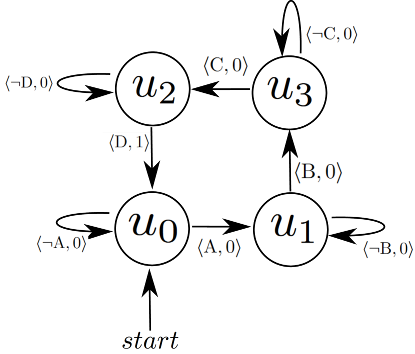
(a) Reward machine

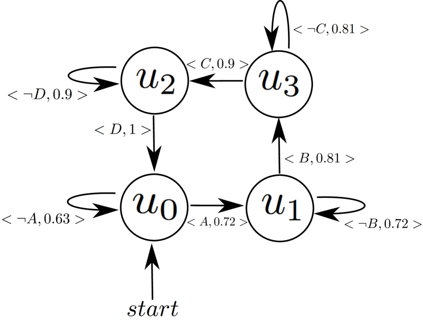
(b) Value iterated RM

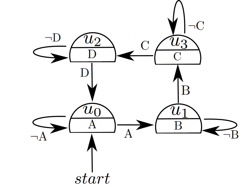
(c) Skill machine

Figure 2: The reward machine, value iterated RM and skill machine for the task "Patrol rooms 1, 2, 3, and 4, without breaking any decoration"

Input :  $\gamma,\alpha,\mathcal{P},L,U,u_{0},F,\delta_{u},\delta_{Q}$

Initialise :  $Q(s,u,a)$

foreach episode do

      Observe initial state $s\in\mathcal{S}$ and get initial $u\leftarrow u_{0}$

      while episode is not done do

           /* Using the composed skill $\delta_{Q}$ in the behaviour policy */

           $a\leftarrow\begin{cases}\operatorname*{arg\,max}\limits_{a\in\mathcal{A}}\left(\max\{\gamma Q(s,u,a),(1-\gamma)\delta_{Q}(s,u,a)\}\right)\quad\text{if}\quad Bernoulli(1-\epsilon)=1\\ \text{a random action}\quad\text{otherwise}\end{cases}$

           Take action $a$ and observe next state $s^{\prime}$

           Get reward $r\leftarrow\delta_{r}(u)(s,a,s^{\prime})$ and the next RM state $u^{\prime}\leftarrow\delta_{u}(u,L(s,a,s^{\prime}))$

          

          $Q(s,u,a)\xleftarrow[]{\alpha}r$ if $s^{\prime}$ is terminal or $u^{\prime}\in F$ else $\left[r+\gamma\max\limits_{a^{\prime}}Q(s^{\prime},u^{\prime},a^{\prime})\right]$

           $s\leftarrow s^{\prime}$

           end while

          

           end foreach

Algorithm 1 Fewshot Q-learning using Skill Machines

4 Experiments

4.1 Discrete Domain

First, we consider the Office Gridworld domain presented in [13] and depicted in Figure 1(a). We use this environment as a multitask domain, consisting of the four tasks described in Table 1.

Task	Description
1	Deliver coffee to the office without breaking any decoration
2	Deliver a mail to the office without breaking any decoration
3	Patrol rooms 1, 2, 3, and 4, without breaking any decoration
4	Deliver coffee and a mail to the office without breaking any decoration

Table 1: Tasks in the office gridworld.

4.1.1 Zero-shot temporal logics

We begin by evaluating how long it takes the agents to learn a policy that can solve all four tasks. The agent will iterate through the tasks, changing from one to the next after each episode. In all of our experiments, we compare the performance of skill machines with that of state-of-the-art RM based learning approaches like counterfactual RMs (CRM)—where the Q-functions are updated with respect to all possible RM transitions from a given environment state—and hierarchical RMs (HRM)—where an agent learns options per RM state that are grounded in the environment states. Note that CRM and HRM are capable of solving the multi-task problem setup because they can use experience from solving one task to update the policies for solving the other tasks. However, skill machines in additional can share both experience between tasks when learning the skill primitives, as well as use the composition of these primitives to generalize zero-shot to more difficult tasks.

We run 25 independent trials and report the average reward per step across the four tasks in Table 1. In addition to learning all four tasks, we also experimented with task $4$ in isolation. For this experiment 25 independent trials were run and the average reward per step computed. In the single task domain, the difference between CRM, HRM, skill machines and Q-Learning should be less severe as CRM, HRM and skill machines now cannot leverage prior knowledge. Thus, the comparison between multi-task and single task learning in this setting will evaluate the benefit of the compositionality afforded by skill machines.

The results of the these two experiments are shown in Figure 3. It is important to note that we train all algorithms for the same amount of time during these experiments and previous work [20] has shown that learning the WVF takes longer than learning task-specific skills. In addition, the skill machines are being used to zero-shot generalise to the office tasks using skill primitives. Thus, using the skill machines in isolation (labelled SM and shown in blue on Figure 3) will provide sub-optimal performance compared to the task specific agents, since the skill machines have not been trained to optimality and are not specialized to the domain. Even under these conditions skill machines perform comparably to HRM+RS in terms of final performance, and due to the amortized nature of learning the WVF will achieve its final rewards from the first epoch.

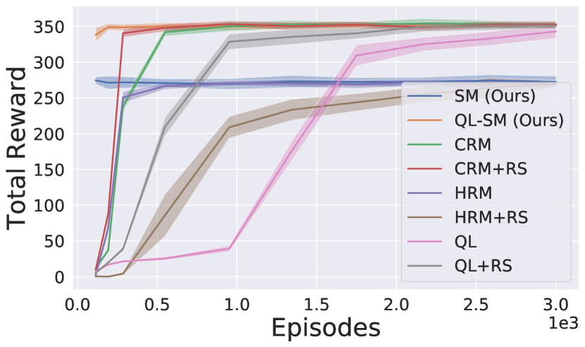
(a) Single task

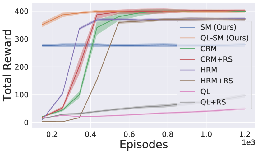
(b) Multiple tasks

Figure 3: Average returns during training in the office gridworld.

4.1.2 Few-shot temporal logics

It is possible to pair the skill machines with a learning algorithm such as Q-Learning to achieve few-shot generalisation. From the results shown in Figure 3 it is apparent that skill machines paired with Q-Learning (labelled QL-SM and shown in orange on Figure 3) achieves the best performance for both the single-task and multi-task setting. Additionally, skill machines with Q-Learning begin with a significantly higher reward and converge on their final performance faster than all benchmarks. The speed of learning is due to the compositionality of the skill primitives with skill machines, and the high final performance is due to the generality of the learned primitives being paired with the domain specific Q-Learner. In sum, skill machines provide fast composition of skills and, when paired with a learning algorithm, achieve optimal performance compared to all benchmarks.

4.2 Moving Targets Domain

We now demonstrate our temporal logic composition approach in a canonical object collection domain with high dimensional pixel observations [20] (Figure 5). The agent here needs to pick up objects of various shapes and colors, and picked objects re-spawn at random empty positions similarly to previous object collection domains [8]. There are 3 object colors—beige, blue, purple—and 2 object shapes—squares, circles. To learn the WVF for a given task primitive, we use the goal oriented Q-learning method of Nangue Tasse et al. [20] where the agent keeps track of reached goals and uses deep Q-learning [19] to update the WVF with respect to all seen goals at every time step.

We first train the agent on 3 base task primitives: pick up blue objects, pick up purple objects, and pick up squares. We then use the learned skill primitives to solve multiple temporal logic tasks. Figure 6 shows the average returns of the optimal policies and SM policies for the 4 tasks described in Table 5. Our results show that even in difficult function approximation settings with sub-optimal skill primitives, the zero-shot policies obtained from skill machines are very close to optimal on average. We also observe that for very hard tasks like task 3 and 4—where the agent must satisfy difficult temporal constraints—, the compounding effect of the sub-optimal policies sometimes lead to failed episodes. In such cases, learning new skills few-shot by leveraging the SM would guarantee convergence to optimal policies as was demonstrated in Section 4.1.2.

[0.25]   [0.6] Task Description 1 Repeatedly pick up any object 2 Repeatedly pick up blue objects, then purple objects, then objects that are neither blue nor purple. 3 Repeatedly pick up blue objects or squares but never blue squares. 4 Repeatedly pick up non-square blue objects then non-blue squares in that order.

Figure 4: Moving-targets domain

Figure 5: Example tasks in the moving-targets domain. Objects re-spawn in random positions when picked.

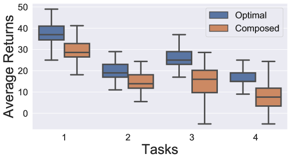
Figure 6: Average returns over 100 runs for tasks in Table 5in the moving-targets domain.

5 Related work

One family of approaches to concurrent composition leverages forms of regularisation to achieve semantically meaningful disjunction [28, 29] or conjunction [11, 12]. Weighted composition has also been demonstrated; for example, Peng et al. [23] learn weights to compose existing policies multiplicatively to solve new tasks. Approaches that leverage the successor feature (SF) framework [6] are capable of solving tasks defined by linear preferences over features [8]. Alver & Precup [1] show that an SF basis can be learned that is sufficient to span the space of tasks under consideration, while Nemecek & Parr [22] determine which policies should be stored in limited memory so as to maximise performance on future tasks. In contrast to these approaches, our framework allows for both concurrent composition (including operators, such as negation, that other approaches do not support) and temporal composition, such as LTL.

A popular way of achieving temporal composition is through the options framework [26, 3]. Here, high-level skills are first discovered and then executed sequentially to solve a task [15, 5]. Barreto et al. [7] leverage the SF and options framework and learn how to linearly combine skills, chaining them sequentially to solve temporal tasks. However, these options-based approaches offer a relatively simple form of temporal composition. By contrast, we are able to solve tasks expressed through regular languages zero-shot, while providing soundness guarantees.

Work has also centred on approaches to defining tasks using human-readable logic operators. For example, Li et al. [17] and Littman et al. [18] specify tasks using LTL, which is then used to generate a standard reward signal for an RL agent to train on. Camacho et al. [9] show how to perform reward shaping given LTL specifications, while Jothimurugan et al. [14] develop a formal language that encodes tasks as sequences, conjunctions and disjunctions of subtasks. This is then used to obtain a shaped reward function that can be used for learning. All of these approaches focus on how an agent can improve learning given such specifications or structure, but we show how an explicitly compositional agent can immediately solve such tasks without further learning using WVFs.

6 Conclusion

We proposed skill machines—finite state machines that can be learned from reward machines—that allow agents to solve extremely complex tasks involving temporal and concurrent composition. We demonstrated how skills can be learned and encoded in a specific form of goal-oriented value function that, when combined with the learned skill machines, are sufficient for solving subsequent tasks without further learning. Our approach guarantees that the resulting policy adheres to the logical task specification, which provides assurances of safety and verifiability to the agent’s decision making, important characteristics that are necessary if we are to ever deploy RL agents in the real world. While the resulting behaviour is provably satisficing, empirical results demonstrate that the agent’s performance is near optimal; further fine-tuning can be performed should optimality be required, which greatly improves the sample efficiency. We see this approach as a step towards truly generally intelligent agents, capable of immediately solving human-specifiable tasks in the real world with no further learning.

References

- Alver & Precup [2022] Alver, S. and Precup, D. Constructing a good behavior basis for transfer using generalized policy updates. In International Conference on Learning Representations, 2022.
- Arjona-Medina et al. [2019] Arjona-Medina, J. A., Gillhofer, M., Widrich, M., Unterthiner, T., Brandstetter, J., and Hochreiter, S. Rudder: Return decomposition for delayed rewards. Advances in Neural Information Processing Systems, 32, 2019.
- Bacon et al. [2017] Bacon, P., Harb, J., and Precup, D. The option-critic architecture. In Thirty-First AAAI Conference on Artificial Intelligence, 2017.
- Badia et al. [2020] Badia, A. P., Piot, B., Kapturowski, S., Sprechmann, P., Vitvitskyi, A., Guo, Z. D., and Blundell, C. Agent57: Outperforming the Atari human benchmark. In International Conference on Machine Learning, pp. 507–517. PMLR, 2020.
- Bagaria & Konidaris [2019] Bagaria, A. and Konidaris, G. Option discovery using deep skill chaining. In International Conference on Learning Representations, 2019.
- Barreto et al. [2017] Barreto, A., Dabney, W., Munos, R., Hunt, J., Schaul, T., van Hasselt, H., and Silver, D. Successor features for transfer in reinforcement learning. In Advances in Neural Information Processing Systems, pp. 4055–4065, 2017.
- Barreto et al. [2019] Barreto, A., Borsa, D., Hou, S., Comanici, G., Aygün, E., Hamel, P., Toyama, D., Mourad, S., Silver, D., Precup, D., et al. The option keyboard: Combining skills in reinforcement learning. Advances in Neural Information Processing Systems, 32, 2019.
- Barreto et al. [2020] Barreto, A., Hou, S., Borsa, D., Silver, D., and Precup, D. Fast reinforcement learning with generalized policy updates. Proceedings of the National Academy of Sciences, 117(48):30079–30087, 2020.
- Camacho et al. [2019] Camacho, A., Icarte, R. T., Klassen, T. Q., Valenzano, R. A., and McIlraith, S. A. LTL and beyond: Formal languages for reward function specification in reinforcement learning. In International Joint Conferences on Artificial Intelligence, volume 19, pp. 6065–6073, 2019.
- Cohen et al. [2021] Cohen, V., Nangue Tasse, G., Gopalan, N., James, S., Gombolay, M., and Rosman, B. Learning to follow language instructions with compositional. In AAAI Fall Symposium Series, 2021.
- Haarnoja et al. [2018] Haarnoja, T., Pong, V., Zhou, A., Dalal, M., Abbeel, P., and Levine, S. Composable deep reinforcement learning for robotic manipulation. In 2018 IEEE International Conference on Robotics and Automation, pp. 6244–6251, 2018.
- Hunt et al. [2019] Hunt, J., Barreto, A., Lillicrap, T., and Heess, N. Composing entropic policies using divergence correction. In International Conference on Machine Learning, pp. 2911–2920, 2019.
- Icarte et al. [2018] Icarte, R. T., Klassen, T., Valenzano, R., and McIlraith, S. Using reward machines for high-level task specification and decomposition in reinforcement learning. In International Conference on Machine Learning, pp. 2107–2116. PMLR, 2018.
- Jothimurugan et al. [2019] Jothimurugan, K., Alur, R., and Bastani, O. A composable specification language for reinforcement learning tasks. Advances in Neural Information Processing Systems, 32, 2019.
- Konidaris & Barto [2009] Konidaris, G. and Barto, A. Skill discovery in continuous reinforcement learning domains using skill chaining. Advances in neural information processing systems, 22, 2009.
- Levine et al. [2016] Levine, S., Finn, C., Darrell, T., and Abbeel, P. End-to-end training of deep visuomotor policies. The Journal of Machine Learning Research, 17(1):1334–1373, 2016.
- Li et al. [2017] Li, X., Vasile, C.-I., and Belta, C. Reinforcement learning with temporal logic rewards. In 2017 IEEE/RSJ International Conference on Intelligent Robots and Systems, pp. 3834–3839. IEEE, 2017.
- Littman et al. [2017] Littman, M., Topcu, U., Fu, J., Isbell, C., Wen, M., and MacGlashan, J. Environment-independent task specifications via gltl. arXiv preprint arXiv:1704.04341, 2017.
- Mnih et al. [2015] Mnih, V., Kavukcuoglu, K., Silver, D., Rusu, A., Veness, J., Bellemare, M., Graves, A., Riedmiller, M., Fidjeland, A., Ostrovski, G., et al. Human-level control through deep reinforcement learning. Nature, 518(7540):529, 2015.
- Nangue Tasse et al. [2020] Nangue Tasse, G., James, S., and Rosman, B. A Boolean task algebra for reinforcement learning. Advances in Neural Information Processing Systems, 33:9497–9507, 2020.
- Nangue Tasse et al. [2022] Nangue Tasse, G., James, S., and Rosman, B. World value functions: Knowledge representation for multitask reinforcement learning. In The 5th Multi-disciplinary Conference on Reinforcement Learning and Decision Making (RLDM), 2022.
- Nemecek & Parr [2021] Nemecek, M. and Parr, R. Policy caches with successor features. In International Conference on Machine Learning, pp. 8025–8033. PMLR, 2021.
- Peng et al. [2019] Peng, X., Chang, M., Zhang, G., Abbeel, P., and Levine, S. MCP: Learning composable hierarchical control with multiplicative compositional policies. In Advances in Neural Information Processing Systems, pp. 3686–3697, 2019.
- Pnueli [1977] Pnueli, A. The temporal logic of programs. In 18th Annual Symposium on Foundations of Computer Science, pp. 46–57. IEEE, 1977.
- Saxe et al. [2017] Saxe, A., Earle, A., and Rosman, B. Hierarchy through composition with multitask LMDPs. International Conference on Machine Learning, pp. 3017–3026, 2017.
- Sutton et al. [1999] Sutton, R., Precup, D., and Singh, S. Between MDPs and semi-MDPs: A framework for temporal abstraction in reinforcement learning. Artificial Intelligence, 112(1-2):181–211, 1999.
- Taylor & Stone [2009] Taylor, M. and Stone, P. Transfer learning for reinforcement learning domains: a survey. Journal of Machine Learning Research, 10:1633–1685, 2009.
- Todorov [2009] Todorov, E. Compositionality of optimal control laws. In Advances in Neural Information Processing Systems, pp. 1856–1864, 2009.
- Van Niekerk et al. [2019] Van Niekerk, B., James, S., Earle, A., and Rosman, B. Composing value functions in reinforcement learning. In International Conference on Machine Learning, pp. 6401–6409, 2019.