Fine-grained Contrastive Learning for Relation Extraction

Abstract

Recent relation extraction (RE) works have shown encouraging improvements by conducting contrastive learning on silver labels generated by distant supervision before fine-tuning on gold labels. Existing methods typically assume all these silver labels are accurate and treat them equally; however, distant supervision is inevitably noisy—some silver labels are more reliable than others. In this paper, we propose fine-grained contrastive learning (FineCL) for RE, which leverages fine-grained information about which silver labels are and are not noisy to improve the quality of learned relationship representations for RE. We first assess the quality of silver labels via a simple and automatic approach we call “learning order denoising,” where we train a language model to learn these relations and record the order of learned training instances. We show that learning order largely corresponds to label accuracy—early-learned silver labels have, on average, more accurate labels than later-learned silver labels. Then, during pre-training, we increase the weights of accurate labels within a novel contrastive learning objective. Experiments on several RE benchmarks show that FineCL makes consistent and significant performance gains over state-of-the-art methods.

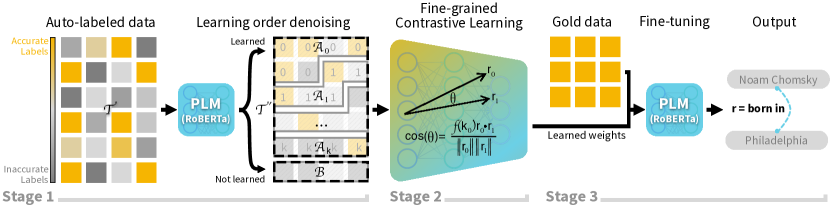
Figure 1: The FineCL framework has three stages: Stage 1: we use distantly supervised data ($\mathcal{T}$) to train a PLM via cross-entropy to collect ordered subsets of learned ($\mathcal{A}$) and not learned ($\mathcal{B}$) instances over $k$ epochs. Stage 2: function $f(k)$ weighs relation instances ($r_{0},r_{1}$) relative to their learning order in a contrastive learning pre-training objective that uses cosine similarity to align similar relations. Stage 3: we adapt the model to a discriminative task.

1 Introduction

Relation extraction (RE), a subtask of information extraction, is a foundational task in Natural Language Processing (NLP). The RE task is to determine a linking relationship between two distinct entities from text, producing fact triples in the form [head, relation, tail]. For example, reading the Wikipedia page on Noam Chomsky, we learn that Noam was “born to Jewish immigrants in Philadelphia,” which corresponds to the fact triple [Noam Chomsky, born in, Philadelphia]. Fact triples play a key role in downstream NLP tasks such as question-answering, search queries, dialog systems, and knowledge-graph completion Xu et al. (2016); Lin et al. (2015); Madotto et al. (2018); Hogan et al. (2021); Li et al. (2014).

Current state-of-the-art RE models leverage a two-phase training: a self-supervised pre-training followed by a supervised fine-tuning. Popular pre-trained language models (PLM) such as BERT Devlin et al. (2019) and RoBERTa Liu et al. (2019) feature a generic pre-training objective, namely masked language modeling (MLM), that allows them to generalize to various downstream tasks. However, recent RE works have shown impressive performance gains by using a pre-training objective designed specifically for relation extraction Soares et al. (2019); Peng et al. (2020); Qin et al. (2021).

Recently, Peng et al. (2020) and Qin et al. (2021) used a contrastive learning loss function to learn relationship representations during pre-training. However, RE-specific pre-training requires large amounts of automatically labeled data obtained trough distant supervision for RE Mintz et al. (2009) which is inherently noisy—not all labels from distantly supervised data are correct. Gao et al. (2021) manually examined distantly supervised relation data and found that a significant ratio, 53%, of the assigned labels were incorrect. Furthermore, distantly supervised labels can go beyond “correct” or “incorrect”—they can have multiple levels of correctness. Consider the following sentences:

1. “Noam Chomsky was born in Philadelphia.”

2. “Noam Chomsky gave a presentation in Philadelphia.”

3. “Raised in the streets of Philadelphia, Noam Chomsky…”

Pairing this text with the Wikidata knowledge graph Vrandečić and Krötzsch (2014), distant supervision labels each sentence as a positive instance of [Noam Chomsky, born in, Philadelphia]; however, only sentence (1) adequately expresses the relationship “born in.” Sentence (2) is incorrectly labeled, and sentence (3) is, arguably, semi-accurate since one may infer that someone was born in the same place they were raised. Conventional contrastive learning for RE does not account for differences in label accuracy—it treats all instances equally. This can be problematic when learning robust and high-quality relationship representations.

This paper proposes a noise-aware contrastive pre-training, Fine-grained Contrastive Learning (FineCL) for RE, that leverages additional fine-grained information about which instances are and are not noisy to produce high-quality relationship representations. Figure 1 illustrates the end-to-end data flow for the proposed FineCL method. We first assess the noise level of all distantly supervised training instances and then incorporate such fine-grained information into the contrastive pre-training. Less noisy, or clean, training instances are weighted more relative to noisy training instances. We then fine-tune the model on gold-labeled data. As we demonstrate in this work, this approach produces high-quality relationship representations from noisy data and then optimizes performance using limited amounts of human-annotated data.

There are several choices of methods to assess noise levels. We select a simple yet effective method we call “learning order denoising” that does not require access to human annotated labels. We train an off-the-shelf language model to predict relationships from distantly supervised data and we record the order of relation instances learned during training. We show that the order in which instances are learned corresponds to the label accuracy of an instance: accurately labeled relation instances are learned first, followed by noisy, inaccurately labeled relation instances.

We leverage learning-order denoising to improve the relationship representations learned during pre-training by linearly projecting the weights of each relation instance corresponding to the order in which the instance was learned. We apply higher weights to relation instances learned earlier in training relative to those learned later in training. We use these weights to inform a contrastive learning loss function that learns to group instances of similar relationships.

We compare our method to leading RE pre-training methods and observe an increase in performance on various downstream RE tasks, illustrating that FineCL produces more informative relationship representations.

The contributions of this work are the following:

• We demonstrate that learning-order denoising is an effective and automatic method for denoising distantly labeled data.

• Applying a denoising strategy to a contrastive learning pre-training objective creates more informative representations, improving performance on downstream tasks.

• We openly provide all code, trained models, experimental settings, and datasets used to substantiate the claims made in this paper.

2 Related Work

Early RE methods featured pattern-based algorithms Califf and Mooney (1997) followed by advanced statistical-based RE methods Mintz et al. (2009); Riedel et al. (2010); Quirk and Poon (2017). Advances in deep learning led to neural-based RE methods Zhang and Wang (2015); Peng et al. (2017); Miwa and Bansal (2016). The transformer Vaswani et al. (2017) enabled the development of wildly successful large pre-trained language models Radford and Narasimhan (2018); Devlin et al. (2019); Liu et al. (2019). At the time of writing, all current leading models in RE leverage large pre-trained language models via a two-step training methodology: a self-supervised pre-training followed by a supervised fine-tuning Xu et al. (2021); Xiao et al. (2021).

	Base Lang. Model	Pre-train objective	RD	ED
BERT	BERT	MLM	$\times$	$\times$
RoBERTa	RoBERTa	MLM	$\times$	$\times$
MTB	BERT	DPS	$\checkmark$	$\times$
CP	BERT	CL + MLM	$\checkmark$	$\times$
ERICABERT	BERT	CL + MLM	$\checkmark$	$\checkmark$
ERICARoBERTa	RoBERTa	CL + MLM	$\checkmark$	$\checkmark$
WCL	BERT	WCL + MLM	$\checkmark$	$\times$
FineCL	RoBERTa	FineCL + MLM	$\checkmark$	$\checkmark$

Table 1: A comparison of RE pre-training methods highlighting the pre-training objective: Mask Language Modeling (MLM), Dot Product Similarity (DPS), Contrastive Learning (CL), Weighted Contrastive Learning (WCL), and Fine-grained Contrastive Learning (FineCL). R_D denotes the presence of relation discrimination in the loss function, and E_D denotes the presence of entity discrimination in the loss function.

Building on BERT Devlin et al. (2019), Soares et al. (2019) proposed MTB, a model featuring a pre-training objective explicitly designed for the task of relation extraction. MTB uses dot product similarly to align pairs of randomly masked entities during pre-training. Its success inspired the development of subsequent RE-specific pre-training methods Peng et al. (2020); Qin et al. (2021). Peng et al. (2020) demonstrated the effectiveness of contrastive learning used to develop relationship representations during pre-training. Their model, named “CP,” featured a pre-training objective that combined a relation discrimination task with BERT’s masked language modeling (MLM) task. Their work inspired ERICA Qin et al. (2021), which expanded the contrastive learning pre-training objective to include entity and relation discrimination, as well as MLM.

Wan et al. (2022) is a recent extension of Peng et al. (2020) that proposes a weighted contrastive learning (WCL) method for RE. The authors first fine-tune BERT to predict relationships using gold training data and then use the fine-tuned model to predict relationships from distantly labeled data. Next, they use the softmax probability of each prediction as a confidence value which they then apply to a weighted contrastive learning function used for pre-training. Lastly, they fine-tune the WCL model on gold training data.

Our work is an extension of ERICA. We introduce a more nuanced RE contrastive learning objective that leverages additional, fine-grained data about which instances are high-quality training signals. Table 1 qualitatively compares recent pre-training methods used for RE.

3 Methods

FineCL for RE consists of three discrete stages: learning order denoising, contrastive pre-training, and supervised adaptation.

3.1 Learning Order Denoising

For learning order denoising, we automatically label large amounts of training data via distant supervision for RE Mintz et al. (2009) which we use to train a PLM to predict relation classes using multi-class cross-entropy loss.

$$\mathcal{L}_{\mathrm{CE}}=-\sum_{i=1}^{N}y_{o,i}\cdot\log\left(p\left(y_{o,i}\right)\right)$$ (1)

Where the number of classes $N$ is the number of relation classes plus one for no relation, $y$ is a binary indicator that is $1$ if and only if $i$ is the correct classification for observation $o$, and $p(y_{o,i})$ is the Softmax probability that observation $o$ is of class $i$.

During training, we record the order of training instances learned. We consider an instance “learned” upon the initial correct prediction. Likewise, an instance is “not learned” if the model fails to predict it correctly during training. Training instances are evaluated by batch within each epoch, exposing the model to all training data points the same number of times. We refer to this method as batch-based learning order.

Thus, the PLM effectively becomes a mapping function that maps all training instances ($\mathcal{T}$) into two subsets: learned ($\mathcal{A}$) and not learned instances ($\mathcal{B}$) such that $\mathcal{A}\bigcup\mathcal{B}=\mathcal{T}^{\prime}$ and $\mathcal{A}\bigcap\mathcal{B}=\emptyset$.

The set of learned instances $\mathcal{A}$ is further divided into non-intersecting subsets of learned instances $\mathcal{A}_{1}$ through $\mathcal{A}_{k}$ where $k$ corresponds to the epoch in which an instance is learned.

$$\mathcal{A}_{0}\bigcup\mathcal{A}_{1}...\bigcup\mathcal{A}_{k}=\mathcal{A}$$ (2)

$$\mathcal{A}_{i}\bigcap\mathcal{A}_{j}=\emptyset\text{ for all }i\neq j$$ (3)

We use $k=15$ epochs, resulting in $k+1$ subsets of instances—$k$ subsets of learned instances plus one subset of not learned instances. Figure 2 shows the percent of total training instances learned per epoch during this phase on the DocRED Yao et al. (2019) distantly labeled training set which contains 100k documents, 1.5M intra- and inter-sentence relation instances, and 96 relation types (not including no relation).

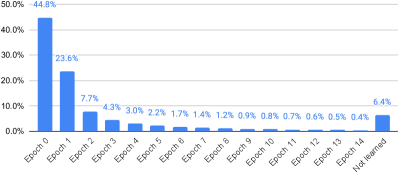
Figure 2: Percent of total training instances learned per epoch when recording batch-based learning order on distantly labeled data from DocRED.

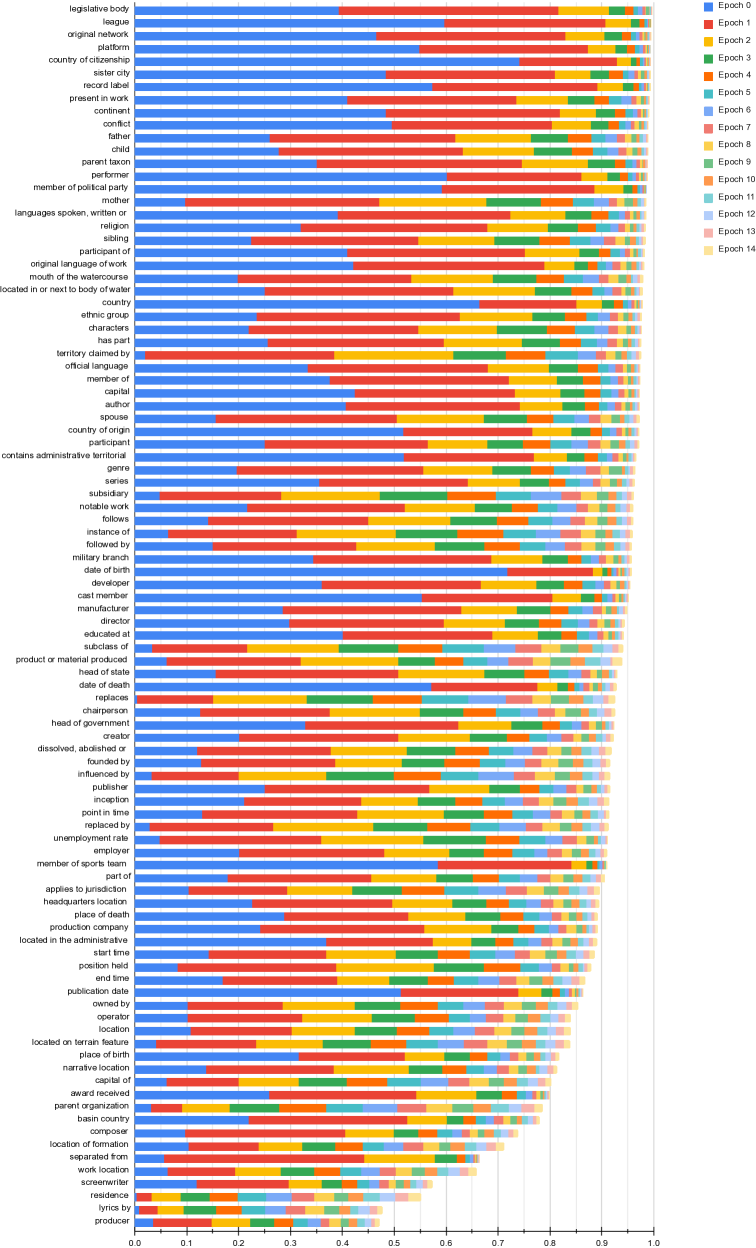
Figure 4: Ratios of instances of learned classes per epoch when recording learning order from distantly supervised DocRED training data. Note, this is before randomized upsampling of underrepresented classes (e.g. lyrics by and producer).

More challenging relation classes may be underrepresented within the set of learned instances. Such minority classes can be problematic during pre-training since unlearned instances are weighted less than learned ones, presenting a challenge for the model to learn informative representations for minority classes. To account for this, we ensure that at least $P\%$ of instances of each relation class is contained within the set of learned instances. During training, we set $P=50$ and observed that 2% of relation classes are underrepresented within the set of learned instances. We upsample underrepresented classes by randomly selecting unlearned instances from the corresponding class, placing them into one of the $k$ subsets of learned instances $\mathcal{A}$. See Figure 4 in the Appendix for a detailed chart showing the ratio of learned instances by relation class in each epoch.

Learning order metadata is then inserted into the original training data $\mathcal{T}$, creating a modified training set $\mathcal{T}^{\prime}$ used for the contrastive pre-training.

3.2 Contrastive Pre-training

This section introduces our pre-training method to learn high-quality entity and relation representations. We first construct informative representation for entities and relationships which we use to implement a three-part pre-training objective that features entity discrimination, relation discrimination, and masked language modeling.

3.2.1 Entity & Relation Representation

We construct entity and relationship representations following ERICA Qin et al. (2021). For the document $d_{i}$, we use a pre-trained language model to encode $d_{i}$ and obtain the hidden states $\{\mathbf{h}_{1},\mathbf{h}_{2},\dots,\mathbf{h}_{|d_{i}|}\}$. Then, mean pooling is applied to the consecutive tokens in entity $e_{j}$ to obtain entity representations. Assuming $n_{\mathrm{start}}$ and $n_{\mathrm{end}}$ are the start index and end index of entity $e_{j}$ in document $d_{i}$, the entity representation of $e_{j}$ is represented as:

$$\mathbf{m}_{e_{j}}=\mathrm{MeanPool}(\mathbf{h}_{n_{\mathrm{start}}},\dots,\mathbf{h}_{n_{\mathrm{end}}}),$$ (4)

To form a relation representation, we concatenate the representations of two entities $e_{j1}$ and $e_{j2}$: $\mathbf{r}_{j1j2}=[\mathbf{e}_{j1};\mathbf{e}_{j2}]$.

3.2.2 Entity Discrimination

For entity discrimination, we use the same method described in ERICA. The goal of entity discrimination ($\mathrm{E_{D}}$) is inferring the tail entity in a document given a head entity and a relation Qin et al. (2021). The model distinguishes the ground-truth tail entity from other entities in the text. Given a sampled instance tuple $t^{i}_{j}k=(d_{i},e_{ij},r^{i}_{jk},e_{ik})$, our model is trained to distinguish the tail entity $e_{ik}$ from other entities in the document $d_{i}$. Specifically, we concatenate the relation name of $r^{i}_{jk}$, the head entity $e_{ij}$ and a special token [SEP] in front of $d_{i}$ to get $d^{*}_{i}$. Then, we encode $d^{*}_{i}$ to get the entity representations using the method from Section 3.2.1. The contrastive learning objective for entity discrimination is formulated as:

$\mathcal{L}_{\mathrm{E_{D}}}=-\sum_{t_{jk}^{i}\in\mathcal{T}^{\prime}}\log\frac{\exp\left(\cos\left(\mathbf{e}_{ij},\mathbf{e}_{ik}\right)/\tau\right)}{\sum_{l=1,l\neq j}^{\left|\mathcal{E}_{i}\right|}\exp\left(\cos\left(\mathbf{e}_{ij},\mathbf{e}_{il}\right)/\tau\right)}$

where $\mathrm{cos}(\cdot,\cdot)$ denotes the cosine similarity between two entity representations and $\tau$ is a temperature hyper-parameter.

3.2.3 Relation Discrimination

To effectively learn representation for downstream task relation extraction, we conduct a Relation Discrimination ($\mathrm{R_{D}}$) task during pre-training. $\mathrm{R_{D}}$ aims to distinguish whether two relations are semantically similar Qin et al. (2021). Existing methods Peng et al. (2020); Qin et al. (2021) require large amounts of automatically labeled data from distant supervision which is noisy because not all sentences will adequately express a relationship.

In this case, the learning order can be introduced to make the model aware of the noise level of relation instances. To efficiently incorporate learning order into the training process, we propose fine-grained, noise-aware relation discrimination.

In this new method, the noise level of all distantly supervised training instances controls the optimization process by re-weighting the contrastive objective. Intuitively, the model should learn more from high-quality, accurately labeled training instances than noisy, inaccurately labeled instances. Hence, we assign higher weights to earlier learned instances from the learning order denoising stage.

In practice, we sample a tuple pair of relation instance $t_{A}=(d_{A},e_{A_{1}},r_{A},e_{A_{2}},k_{A})$ and $t_{B}=(d_{B},e_{B_{1}},r_{B},e_{B_{2}},k_{B})$ from $\mathcal{T}^{\prime}$ and $r_{A}=r_{B}$, where $d$ is a document; $e$ is a entity in $d$; $r$ is the relationship between two entities and $k$ is the first learned order introduced in Section 3.1. Using the method mentioned in Section 3.2.1, we obtain the positive relation representations $\mathbf{r}_{t_{A}}$ and $\mathbf{r}_{t_{B}}$. To discriminate positive examples from negative ones, the fine-grained $\mathrm{R_{D}}$ is defined as follows:

$$\mathcal{L}_{\mathrm{R_{D}}} =-\sum_{t_{A},t_{B}\in\mathcal{T}^{\prime}}f(k_{A})\log\frac{\exp\left(\cos\left(\mathbf{r}_{t_{A}},\mathbf{r}_{t_{B}}\right)/\tau\right)}{\mathcal{Z}},$$ (5)

$$\mathcal{Z} =\sum_{t_{C}\in\mathcal{T}^{\prime}/\left\{t_{A}\right\}}^{N}f(k_{C})\exp\left(\cos\left(\mathbf{r}_{t_{A}},\mathbf{r}_{t_{C}}\right)/\tau\right)$$

where $\mathrm{cos}(\cdot,\cdot)$ denotes the cosine similarity; $\tau$ is the temperature; $N$ is a hyper-parameter and $t_{C}$ is a negative instance ($r_{A}\neq r_{C}$) sampled from $\mathcal{T}^{\prime}$. Relation instances $t_{A}$ and $t_{C}$ are re-weighted by function $f$ which is defined as:

$$f(k)=\alpha^{\frac{k_{\mathrm{max}}-k}{k_{\mathrm{max}}-k_{\mathrm{min}}}},$$ (6)

where $\alpha$ ($\alpha>1$) is a hyper-parameter of the function $f$; $\mathrm{max}$ and $\mathrm{min}$ are maximum and minimum first-learned order, respectively. We increase the weight of negative $t_{C}$ if it is a high-quality training instance (i.e., $k$ is small). Because all positives and negatives are discriminated from instance $t_{A}$, we control the overall weight by the learning order $k_{A}$.

3.2.4 Overall Objective

We include the MLM task Devlin et al. (2019) to avoid catastrophic forgetting of language understanding McCloskey and Cohen (1989) and construct the following overall objective for FineCL:

$$\mathcal{L}_{FineCL}=\mathcal{L}_{E_{D}}+\mathcal{L}_{R_{D}}+\mathcal{L}_{MLM}$$ (7)

3.3 Supervised Adaptation

The primary focus of our work is to improve relationship representations learned during pre-training and, in doing so, improve performance on downstream RE tasks. To illustrate the effectiveness of our pre-training method, we use cross-entropy loss, as described in equation 1, to fine-tune our pre-trained FineCL model on document-level and sentence-level RE tasks.

4 Experiments

4.1 Learning Order as Noise Level Hypothesis

We first seek to confirm our hypothesis that the learning order automatically orders distantly supervised data from clean, high-quality instances to noisy, low-quality instances. However, given the large amount of pre-training data, statistically significant confirmation via manual annotation is prohibitively expensive. So, we devise the following experiment to test our hypothesis in lieu of a significant manual annotation effort.

We begin with the assumption that a model trained on a dataset without noise will perform better than a model trained on a dataset with noise. Suppose learning order denoising successfully orders instances relative to their noise; then, we should observe a boost in performance by training on a subset of early-learned instances compared to a model trained on the complete, noisy dataset.

As reported by Gao et al. (2021), up to 53% of relation instances labeled via distant supervision are incorrect. Using this estimation, we attempt to use learning order denoising to remove the roughly 50% of instances that are noisy instances from the DocRED’s distantly supervised training set. To do this, we first obtain the learning order of relation instances using the methodology described in Section 3.1. Without loss of generalization, we choose RoBERTa Liu et al. (2019), specifically the roberta-base checkpoint, as the base model to develop the order of learned instances.

Learning order	Training set	Training set size	F1
None	$\mathcal{T}$	100%	45.8
Batch-based	$\mathcal{T}_{\mathcal{A}_{0}^{B}}$	45.0%	46.6
Epoch-based	$\mathcal{T}_{\mathcal{A}_{0}^{E}}$	64.9%	46.0

Table 2: Results comparing performance on the DocRED test set using trimmed sets of distantly supervised training data. The batch-based and epoch-based training sets consist of training instances determined by the instances learned within the first epoch using the respective learning order collection methods.

We observe that the set of training instances learned via batch-based learning order in the first epoch, $\mathcal{A}_{0}^{B}$, consists of 45% of the total training instances. We use $\mathcal{A}_{0}^{B}$ to construct a trimmed training set $\mathcal{T}_{\mathcal{A}_{0}^{B}}$. We then compare performance in two settings: (1) RoBERTa trained with the complete distantly supervised training dataset $\mathcal{T}$ and (2) RoBERTa trained on the trimmed, denoised training data $\mathcal{T}_{\mathcal{A}_{0}^{B}}$. Table 2 reports the results of this experiment. Significantly, the denoised training set consisting of only 45% training data outperforms the baseline model.

We also conduct an informal manual analysis of the learning order. We randomly selected 120 instances from the first six training epochs—60 correctly, and 60 incorrectly predicted instances. We find that 93% of the correct predictions have accurate labels within the first three epochs. However, in epochs 4 through 6, label accuracy drops to 53% among correct predictions. Furthermore, we find a relatively low label accuracy of 50% from the first three epochs of incorrect predictions, illustrating that the model struggles to learn noisy instances compared to clean instances early in training. We use these results and the results presented in Table 2 to argue that learning order successfully orders instances from clean, high-quality to noisy, low-quality instances.

4.2 Learning Order: Batch- vs. Epoch-based

We experiment with two methods of collecting learning order data: batch-based and epoch-based (see Appendix A.1 for pseudo-code describing these methods).
Batch-based: As previously mentioned, for batch-based learning order we collect learned instances per batch across each epoch during training. However, we recognize that this may bias the set of learned instances by the random batch for which they are selected. For example, accurately labeled relation instances selected for the first few batches during training may not be predicted correctly because the model has not learned much.
Epoch-based: To reduce potential selection order bias from batch-based learning order, we experiment with epoch-based learning order by evaluating the model on the entire training set at the end of each epoch. We rerun the experiment detailed in Section 4.1 using epoch-based learning order to construct the trimmed dataset $\mathcal{T}_{\mathcal{A}_{0}^{E}}$ and present the results in Table 2.

Using epoch-based learning order, we observe that the model learns 64.9% of the training instances within the first epoch, an increase compared to the 45.0% of learned instances from batch-based learning order. However, training RoBERTa on the epoch-based training subset, we obtain an F1 score of 46.0, which under-performs relative to the 46.6 F1 score from the batch-based learning order experiment. We hypothesize that, while epoch-based learning order may capture more learned instances, it leads to noisier instances leaking into the sets of learned data because the model is more prone to simply memorizing noisy labels encountered previously in the epoch.

Note that we do not use DocRED’s human-annotated training data in these learning order experiments. Instead, we train on the distantly supervised training data and test on human-annotated data. This is done to assess the quality of the various subsets of distantly labeled data. It is why the performance of these tests is considerably lower than the results from the experiments in Section 4.4 that leverage human-annotated training data.

4.3 Pre-training Details

To ensure a fair comparison and highlight the effectiveness of FineCL, we align our pre-training data and settings to those used by ERICA. The ERICA pre-training dataset is constructed using distant supervision for RE by pairing documents from Wikipedia (English) with the Wikidata knowledge graph. This distantly labeled dataset creation method mirrors the method used to create the distantly labeled training set in DocRED but differs in that it is much larger and more diverse. It contains 1M documents, 7.2M relation instances, and 1040 relation types compared to DocRED’s 100k documents, 1.5M relation instances, and 96 relation types (not including no relation). Additional checks are performed to ensure no fact triples overlap between the training data and the test sets of the various downstream RE tasks. Detailed pre-training settings can found in Appendix A.2.

Size	1%		10%		100%
Metrics	F1	IgF1	F1	IgF1	F1	IgF1
CNN*	-	-	-	-	42.3	40.3
BiLSTM*	-	-	-	-	51.1	50.3
HINBERT*	-	-	-	-	55.6	53.7
CorefBERT*	32.8	31.2	46.0	43.7	57.0	54.5
SpanBERT*	32.2	30.4	46.4	44.5	57.3	55.0
ERNIE*	26.7	25.5	46.7	44.2	56.6	54.2
MTB*	29.0	27.6	46.1	44.1	56.9	54.3
CP*	30.3	28.7	44.8	42.6	55.2	52.7
BERT	19.9	18.8	45.2	43.1	56.6	54.4
RoBERTa	29.6	27.9	47.6	45.7	58.2	55.9
ERICABERT	22.9	21.7	48.5	46.4	57.4	55.2
ERICARoBERTa	30.0	28.2	50.1	48.1	59.1	56.9
WCLRoBERTa	22.3	20.8	49.4	47.5	58.5	56.2
FineCL	33.2	31.2	50.3	48.3	59.5	57.1

Table 3: F1-micro scores reported on the DocRED test set. IgF1 ignores performance on fact triples in the test set overlapping with triples in the train/dev sets. (* denotes performance as reported in Qin et al. (2021); all other numbers are from our implementations).

4.4 Relation Extraction

Document-level RE: To assess our framework’s ability to extract document-level relations, we report performance on DocRED Yao et al. (2019). We compare our model to the following baselines: (1) CNN Zeng et al. (2014), (2) BiLSTM Hochreiter and Schmidhuber (1997), (3) BERT Devlin et al. (2019), (4) RoBERTa Liu et al. (2019), (5) MTB Soares et al. (2019), (6) CP Peng et al. (2020), (7 & 8) ERICA_BERT & ERICA_RoBERTa Qin et al. (2021), (9) WCL Wan et al. (2022). We fine-tune the pre-trained models on DocRED’s human-annotated train/dev/test splits (see Appendix A.3.1 for detailed experimental settings). We implement WCL with identical settings from our other pre-training experiments and, for fair comparison, we use RoBERTa instead of BERT as the base model for WCL, given the superior performance we observe from RoBERTa in all other experiments. Table 3 reports performance across multiple data reduction settings (1%, 10%, and 100%), using an overall F1-micro score and an F1-micro score computed by ignoring fact triples in the test set that overlap with fact triples in the training and development splits. We observe that FineCL outperforms all baselines in all experimental settings, offering evidence that FineCL produces better relationship representations from noisy data.

Given that learning-order denoising weighs earlier learned instances over later learned instances, FineCL may be biased towards easier, or common relation classes. The increase in F1-micro performance may result from improved predictions on common relation classes at the expense of predictions on rare classes. To better understand the performance gains, we also report F1-macro and F1-macro weighted in Table 4. The results show that FineCL outperforms the top baselines in both F1-macro metrics indicating that, on average, our method improves performance across all relation classes. However, the low F1-macro scores from all the models highlight an area for improvement—future pre-trained RE models should focus on improving performance on long-tail relation classes.

Metric	F1-macro	F1-macro-weighted
BERT	37.3	54.9
RoBERTa	39.6	56.9
ERICABERT	37.9	55.8
ERICARoBERTa	40.1	57.8
WCLRoBERTA	39.9	57.2
FineCL	40.7	58.2

Table 4: F1-macro and F1-macro-weighted scores reported from the DocRED test set.

Dataset	TACRED			SemEval
Size	1%	10%	100%	1%	10%	100%
MTB*	35.7	58.8	68.2	44.2	79.2	88.2
CP*	37.1	60.6	68.1	40.3	80.0	88.5
BERT	22.2	53.5	63.7	41.0	76.5	87.8
RoBERTa	27.3	61.1	69.3	43.6	77.7	87.5
ERICABERT	34.9	56.0	64.9	46.4	79.8	88.1
ERICARoBERTa	41.1	61.7	69.5	50.3	80.9	88.4
WCLRoBERTA	37.6	61.3	69.7	47.0	80.0	88.3
FineCL	43.7	62.7	70.3	51.2	81.0	88.7

Table 5: F1-micro scores reported from the TACRED and SemEval test sets (* denotes performance as reported in Qin et al. (2021); all other numbers are from our implementations).

Sentence-level RE: To assess our framework’s ability to extract sentence-level relations, we report performance on TACRED Zhang et al. (2017) and SemEval-2010 Task 8 Hendrickx et al. (2010). We compare our model to MTB, CP, BERT, RoBERTa, ERICA_BERT, ERICA_RoBERTa, and WCL (see Appendix A.3.2 for detailed experimental settings). Table 5 reports F1 scores across multiple data reduction settings (1%, 10%, 100%). Again, we observe that FineCL outperforms all baselines in all settings.

5 Ablation Studies

We conduct a suite of ablation experiments to understand how learning order denoising affects the quality of relationship representations learned during pre-training. We note that the FineCL method is identical to ERICA when we remove fine-grained data and treat all instances equally. As such, ERICA can be considered an ablation experiment of FineCL without fine-grained data.

5.1 Learning Order Epochs

In our first ablation experiment, we vary the number of training epochs ($k$) used to obtain learning order data to determine how the different amounts of batch-based learning order data affect pre-training. We test $k=\{1,3,5,10,15\}$ as well as a baseline that does not use learning order denoising. To reduce the high computational requirements for pre-training, we use a shortened pre-training for these experiments where we pre-train for 1000 training steps compared to the full 6000 step training used for our main experiments. We then fine-tune the models using the same settings described in Section 4.4. Notably, our pre-trained model trained at 1000 steps achieves an F1 score of 59.0, which is reasonably close to the 59.5 F1 score from the FineCL trained for 6000 steps. Table 6 contains the results from this ablation experiment. We observe that $k=15$ epochs of learned instances produce the best performance, indicating that a more extensive set of learned instances produces better relationship representations.

Epochs of learning order data	% Learned	F1	IgF1
Baseline	N/A	58.7	56.5
1 Epoch	45	58.6	56.4
3 Epochs	76	58.6	56.3
5 Epochs	83	58.7	56.5
10 Epochs	92	58.8	56.6
15 Epochs	94	59.0	56.7

Table 6: Ablation experiment results on the DocRED test set with pre-trained models that use learning order data obtained with various training durations. Percent learned refers to the percent of training instances learned in the set of learned instances ($\mathcal{A}$). “Baseline” is a pre-trained model that does not leverage learning order (i.e., all instances are weighted equally during pre-training).

5.2 Different Learning Order Models

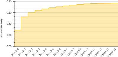
Figure 3: Cumulative Jaccard Similarity between sets of learned instances by epoch from RoBERTa and SSAN using distantly labeled training data from DocRED.

We chose the RoBERTa base model for the first stage of our FineCL framework to reduce the adoption barrier for our methodology. Popular pre-trained models such as roberta-base are easy to implement and require fewer resources compared to larger state-of-the-art (SOTA) RE models. However, given that RoBERTa is not a leading RE model, we seek to answer the question—how do sets of learned training instances differ between RoBERTa and the SOTA RE model? At the time of writing, the leading RE model on DocRED is the SSAN model Xu et al. (2021). Therefore, we compare sets of learned instances from SSAN ($\mathcal{A}^{S}$) and RoBERTa ($\mathcal{A}^{R}$) by epoch ($k$) using a cumulative Jaccard Similarity Index:

$$J(\mathcal{A}^{R},\mathcal{A}^{S})=\sum_{i=0}^{k}\frac{|\mathcal{A}_{i}^{R}\cap\mathcal{A}_{i}^{S}|}{|\mathcal{A}_{i}^{R}\cup\mathcal{A}_{i}^{S}|}$$

Figure 3 plots the cumulative Jaccard Similarity Index (JSI) between sets of learned instances from RoBERTa and SSAN. The total cumulative JSI between the two models after $k=15$ epochs is 0.771, showing high similarity between sets of learned instances. While the sets are not perfectly aligned, we argue that this high similarity justifies using the smaller and more convenient RoBERTa model in determining learning order. We leave a more thorough examination of the differences in sets of learned instances obtained using various RE models to future work and present our findings as a proof of concept, demonstrating that obtaining learning order from relatively small and convenient language models is sufficient in improving representations learned during pre-training.

5.3 Performance Relative to Class Difficulty

Metric	F1-micro
BERT	32.9
RoBERTa	35.8
ERICABERT	34.7
ERICARoBERTa	34.4
WCLRoBERTA	35.7
FineCL	36.1

Table 7: F1-micro scores on a subset of difficult relation classes from the DocRED dataset.

As mentioned in Section 3.1, it is possible that learning-order denoising biases the model to easier, common relation classes, as easier classes may be over-represented in the set of learned instances. To understand the effectiveness of our approach relative to class difficulty, we assess the end-to-end performance of FineCL on a set of difficult relation classes.

We recognize that there are multiple ways to define a “difficult” relation class. Difficult classes can be classes with few training instances, classes with a significant number of inaccurate or semi-accurate labels, or classes that suffer from low overall accuracy after training completes. For this ablation study, we define the set of difficult relation classes as classes that attain relatively low accuracy from the training in Stage 1 of FineCL. We claim that any class which achieves less than 80% accuracy after Stage 1 training completes is a “difficult” relation class. This subset of the lowest-performing classes from the DocRED dataset makes up 24% of all the classes in the dataset.

We compare the end-to-end performance of FineCL to baselines that do not leverage fine-grained contrastive learning on the set of difficult relation classes. Table 7 contains the results from this experiment. We observe that FineCL achieves an F1 score of 36.1% on the subset of difficult classes compared to the best-performing baseline which achieves 35.8%. We argue that these results, as well as the results from Table 4, offer evidence that the FineCL approach is capable of improving performance on both difficult classes as well as easy classes. However, the low overall performance from all models on difficult classes highlights an area for future work.

6 Conclusion

In this work, we expand on contrastive learning for relation extraction by introducing Fine-grained Contrastive Learning for RE—a method that uses additional, fine-grained information about distantly supervised training data to improve relationship representations learned during pre-training. These improved representations lead to increases in performance across a variety of downstream RE tasks. This report shows that learning order denoising effectively and automatically orders distantly supervised training data from clean to noisy instances. In future work, we hope to explore the usefulness of this method when applied to manually annotated data where learning order may instead reflect the level of difficulty of training instances. This could be an easy and automatic way to introduce curricula learning within the fine-tuning training phase. We also intend to explore the pairing of other denoising methods with FineCL.

7 Limitations

The limitations of our method are as follows:

1. Our method requires access to a robust knowledge graph to define the concepts and the relationships for distant supervision.

2. Our method minimizes the need for but still requires human-annotated data, which is both expensive and time-consuming to create.

3. The low F1-macro scores of our model and all other leading RE models highlight the need to improve performance on long-tail relation classes in future works.

Appendix A Appendix

A.1 Learning order methods: batch- vs epoch-based

1 k = 15 epochs

2 for $i=0$ to $k$ do

3       foreach batch of training data do

4             predictions $\leftarrow$ model(batch)

5             $\mathcal{A}_{i}$.insert(correct predictions)

6             Calculate loss

7             Back propagate

8            

Algorithm 1 Batch-based learning order

1 k = 15 epochs

2 for $i=0$ to $k$ do

3       foreach batch of training data do

4             Calculate loss

5             Back propagate

6            

7      predictions $\leftarrow$ model(all training data)

8       $\mathcal{A}_{i}$.insert(correct predictions)

9      

Algorithm 2 Epoch-based learning order

A.2 Pre-training Settings

We initialize our model with roberta-base released by Huggingface. The optimizer is AdamW and we set the learning rate to $3\times 10^{-5}$, weight decay to $1\times 10^{-5}$, batch size to 768 and temperature $\tau$ to $5\times 10^{-2}$. The hyper-parameter $\alpha$ that controls the weights of contrastive learning is $e$ (the base of natural logarithm). We randomly sample 64 negatives for each document. We train our model with 3 NVIDIA Tesla V100 GPUs for 6,000 steps.

A.3 Downstream Training Settings

A.3.1 DocRED

We fine-tune our model on DocRED using the following settings: batch size=32, epochs=200, max sequence length=512, gradient accumulation steps=1, learning rate=4e-5, weight decay=0, adam epsilon=1e-8, max gradient norm=1.0, hidden size=768, and a seed=42. Results are reported on the official DocRED test set as an average of three runs.

A.3.2 SemEval and TACRED

We fine tune our moodel on SemEval and TACRED using the following settings: batch size=64, max sequence length=100, learning rate=5e-5, adam epsilon=1e-8, weight decay=1e-5, max gradient norm=1.0, warm up steps=500, and hidden size=768. We ran tests on training proportions 0.01/0.1/1.0 using 80/20/8 epochs and a dropout of 0.2/0.1/0.35, respectively.

Results are reported as an average of five runs using the following seed values: 42, 43, 44, 45, and 46.

References

- Califf and Mooney (1997) Mary Elaine Califf and Raymond J. Mooney. 1997. Relational learning of pattern-match rules for information extraction. In CoNLL.
- Devlin et al. (2019) Jacob Devlin, Ming-Wei Chang, Kenton Lee, and Kristina Toutanova. 2019. Bert: Pre-training of deep bidirectional transformers for language understanding. In NAACL.
- Gao et al. (2021) Tianyu Gao, Xu Han, Keyue Qiu, Yuzhuo Bai, Zhiyu Xie, Yankai Lin, Zhiyuan Liu, Peng Li, Maosong Sun, and Jie Zhou. 2021. Manual evaluation matters: Reviewing test protocols of distantly supervised relation extraction. In FINDINGS.
- Hendrickx et al. (2010) Iris Hendrickx, Su Nam Kim, Zornitsa Kozareva, Preslav Nakov, Diarmuid Ó Séaghdha, Sebastian Padó, Marco Pennacchiotti, Lorenza Romano, and Stan Szpakowicz. 2010. SemEval-2010 task 8: Multi-way classification of semantic relations between pairs of nominals. In Proceedings of the 5th International Workshop on Semantic Evaluation, pages 33–38, Uppsala, Sweden. Association for Computational Linguistics.
- Hochreiter and Schmidhuber (1997) Sepp Hochreiter and Jürgen Schmidhuber. 1997. Long short-term memory. Neural Computation, 9:1735–1780.
- Hogan et al. (2021) William P Hogan, Molly Huang, Yannis Katsis, Tyler Baldwin, Ho-Cheol Kim, Yoshiki Baeza, Andrew Bartko, and Chun-Nan Hsu. 2021. Abstractified multi-instance learning (AMIL) for biomedical relation extraction. In 3rd Conference on Automated Knowledge Base Construction.
- Li et al. (2014) Zhixu Li, Mohamed A. Sharaf, Laurianne Sitbon, Xiaoyong Du, and Xiaofang Zhou. 2014. Core: A context-aware relation extraction method for relation completion. IEEE Transactions on Knowledge and Data Engineering, 26:836–849.
- Lin et al. (2015) Yankai Lin, Zhiyuan Liu, Maosong Sun, Yang Liu, and Xuan Zhu. 2015. Learning entity and relation embeddings for knowledge graph completion. In AAAI.
- Liu et al. (2019) Yinhan Liu, Myle Ott, Naman Goyal, Jingfei Du, Mandar Joshi, Danqi Chen, Omer Levy, Mike Lewis, Luke Zettlemoyer, and Veselin Stoyanov. 2019. Roberta: A robustly optimized bert pretraining approach. ArXiv, abs/1907.11692.
- Madotto et al. (2018) Andrea Madotto, Chien-Sheng Wu, and Pascale Fung. 2018. Mem2seq: Effectively incorporating knowledge bases into end-to-end task-oriented dialog systems. In ACL.
- McCloskey and Cohen (1989) Michael McCloskey and Neal J. Cohen. 1989. Catastrophic interference in connectionist networks: The sequential learning problem. Psychology of Learning and Motivation, 24:109–165.
- Mintz et al. (2009) Mike D. Mintz, Steven Bills, Rion Snow, and Dan Jurafsky. 2009. Distant supervision for relation extraction without labeled data. In ACL.
- Miwa and Bansal (2016) Makoto Miwa and Mohit Bansal. 2016. End-to-end relation extraction using lstms on sequences and tree structures. ArXiv, abs/1601.00770.
- Peng et al. (2020) Hao Peng, Tianyu Gao, Xu Han, Yankai Lin, Peng Li, Zhiyuan Liu, Maosong Sun, and Jie Zhou. 2020. Learning from context or names? an empirical study on neural relation extraction. In EMNLP.
- Peng et al. (2017) Nanyun Peng, Hoifung Poon, Chris Quirk, Kristina Toutanova, and Wen tau Yih. 2017. Cross-sentence n-ary relation extraction with graph lstms. Transactions of the Association for Computational Linguistics, 5:101–115.
- Qin et al. (2021) Yujia Qin, Yankai Lin, Ryuichi Takanobu, Zhiyuan Liu, Peng Li, Heng Ji, Minlie Huang, Maosong Sun, and Jie Zhou. 2021. Erica: Improving entity and relation understanding for pre-trained language models via contrastive learning. In ACL.
- Quirk and Poon (2017) Chris Quirk and Hoifung Poon. 2017. Distant supervision for relation extraction beyond the sentence boundary. In EACL.
- Radford and Narasimhan (2018) Alec Radford and Karthik Narasimhan. 2018. Improving language understanding by generative pre-training. In OpenAI.
- Riedel et al. (2010) Sebastian Riedel, Limin Yao, and Andrew McCallum. 2010. Modeling relations and their mentions without labeled text. In ECML/PKDD.
- Soares et al. (2019) Livio Baldini Soares, Nicholas FitzGerald, Jeffrey Ling, and Tom Kwiatkowski. 2019. Matching the blanks: Distributional similarity for relation learning. ArXiv, abs/1906.03158.
- Vaswani et al. (2017) Ashish Vaswani, Noam M. Shazeer, Niki Parmar, Jakob Uszkoreit, Llion Jones, Aidan N. Gomez, Lukasz Kaiser, and Illia Polosukhin. 2017. Attention is all you need. ArXiv, abs/1706.03762.
- Vrandečić and Krötzsch (2014) Denny Vrandečić and Markus Krötzsch. 2014. Wikidata: A free collaborative knowledgebase. Commun. ACM, 57(10):78–85.
- Wan et al. (2022) Zhen Wan, Fei Cheng, Qianying Liu, Zhuoyuan Mao, Haiyue Song, and Sadao Kurohashi. 2022. Relation extraction with weighted contrastive pre-training on distant supervision.
- Xiao et al. (2021) Yuxin Xiao, Zecheng Zhang, Yuning Mao, Carl Yang, and Jiawei Han. 2021. Sais: Supervising and augmenting intermediate steps for document-level relation extraction. ArXiv, abs/2109.12093.
- Xu et al. (2021) Benfeng Xu, Quan Wang, Yajuan Lyu, Yong Zhu, and Zhendong Mao. 2021. Entity structure within and throughout: Modeling mention dependencies for document-level relation extraction. In AAAI.
- Xu et al. (2016) Kun Xu, Siva Reddy, Yansong Feng, Songfang Huang, and Dongyan Zhao. 2016. Question answering on freebase via relation extraction and textual evidence. Proceedings of the 54th Annual Meeting of the Association for Computational Linguistics (Volume 1: Long Papers).
- Yao et al. (2019) Yuan Yao, Deming Ye, Peng Li, Xu Han, Yankai Lin, Zhenghao Liu, Zhiyuan Liu, Lixin Huang, Jie Zhou, and Maosong Sun. 2019. Docred: A large-scale document-level relation extraction dataset. ArXiv, abs/1906.06127.
- Zeng et al. (2014) Daojian Zeng, Kang Liu, Siwei Lai, Guangyou Zhou, and Jun Zhao. 2014. Relation classification via convolutional deep neural network. In Proceedings of COLING 2014, the 25th International Conference on Computational Linguistics: Technical Papers, pages 2335–2344, Dublin, Ireland. Dublin City University and Association for Computational Linguistics.
- Zhang and Wang (2015) Dongxu Zhang and Dong Wang. 2015. Relation classification via recurrent neural network. ArXiv, abs/1508.01006.
- Zhang et al. (2017) Yuhao Zhang, Victor Zhong, Danqi Chen, Gabor Angeli, and Christopher D. Manning. 2017. Position-aware attention and supervised data improve slot filling. In Proceedings of the 2017 Conference on Empirical Methods in Natural Language Processing (EMNLP 2017), pages 35–45.