Bayesian multiscale analysis of the Cox model

Supplement to “Bayesian multiscale analysis of the Cox model”

Abstract

Piecewise constant priors are routinely used in the Bayesian Cox proportional hazards model for survival analysis. Despite its popularity, large sample properties of this Bayesian method are not yet well understood. This work provides a unified theory for posterior distributions in this setting, not requiring the priors to be conjugate. We first derive contraction rate results for wide classes of histogram priors on the unknown hazard function and prove asymptotic normality of linear functionals of the posterior hazard in the form of Bernstein–von Mises theorems. Second, using recently developed multiscale techniques, we derive functional limiting results for the cumulative hazard and survival function. Frequentist coverage properties of Bayesian credible sets are investigated: we prove that certain easily computable credible bands for the survival function are optimal frequentist confidence bands. We conduct simulation studies that confirm these predictions, with an excellent behavior particularly in finite samples. Our results suggest that the Bayesian approach can provide an easy solution to obtain both the coefficients estimate and the credible bands for survival function in practice.

Abstract

In this supplemental, we include the proofs for the results stated in the main paper. We also provide a summary of contents and the background on the Cox model.

and

t1The author gratefully acknowledges the support from the Fondation Sciences Mathématiques de Paris postdoctoral fellowship. t2The author gratefully acknowledges support from the Institut Universitaire de France (IUF) and from the ANR grant ANR-17-CE40-0001 (BASICS).

1 Introduction

The Cox proportional hazards model (hereafter, the Cox model) introduced by Cox (1972) is one of the most popular regression models for survival analysis. It is a semiparametric model with two sets of unknown parameters: the regression coefficients, which measure the correlation between the covariates and the explanatory variables, and the baseline hazard, a nonparametric quantity, which describes the risk of events happening within given time intervals at baseline levels conditional on the covariates. A commonly used approach to estimate the two parameters takes two steps: first estimate the regression coefficients from the Cox partial likelihood (Cox, 1972) and then derive the estimated cumulative hazard function (known as the Breslow estimator (Breslow, 1972)) through maximizing the full likelihood via plugging-in the estimated value of the regression coefficients.

In the past few decades, Bayesian methods for the Cox model have been widely applied for analyzing datasets in, e.g., astronomy (Isobe et al., 1986), medical and genetics studies (Li and Ma, 2013), and engineering (Equeter et al., 2020). An advantage of the Bayesian approach is that uncertainty quantification for the parameters of interest is in principle straightforward to obtain once posterior samples are available. Contrary to the standard two-step procedure mentioned above, the Bayesian approach provides estimates for the joint distribution of all parameters, which enables to capture dependencies: in particular, as one of the practical applications considered below, one can derive meaningful uncertainty quantification simultaneously for the Cox model parameter and functionals of the hazard rate (e.g. its mean, or the value of the survival function at a point) from corresponding credible sets, in particular automatically capturing the (optimal ‘efficient’) dependence structure.

The prior for the hazard function needs to be chosen carefully, as it is a nonparametric quantity. Two main common approaches to place a prior on hazards have been considered in the literature. A first approach puts a prior on the cumulative hazard function, modeling this quantity rather than the hazard itself. A prominent example is the family of neutral to the right process priors, which includes the Beta process prior (Hjort, 1990; Damien et al., 1996), the Gamma process prior (Kalbfleisch, 1978; Burridge, 1981), and the Dirichlet process prior (Florens et al., 1999) as special cases. A second approach, which is the one we follow here, is to put a prior on the baseline hazard function. A commonly used family is that of piecewise constant priors (Ibrahim et al., 2001). The latter approach is particularly attractive, first because it allows for inference on the hazard rate (assuming it exists), and second because in practice the follow-up period is often split into several intervals, with the hazard rate taking a distinct constant value on each sub-interval, making the output of the method easy to interpret for practitioners.

One primary goal of the paper is to validate the practical use of Bayesian credible sets for inference on the Cox model’s unknown parameters, for instance credible bands for the survival function conditional on the covariates. Indeed, practitioners often treat Bayesian credible sets as confidence sets. Before discussing the possible mathematical validity of this practice, let us conduct a simple illustrative simulation study (see Section 4 for a detailed description of the simulation setting).

From data simulated from the Cox model, suppose we want to make inference on the survival function conditional on $z$, which gives the probability that a patient survives past a certain time $t$ given a covariate $z\in\mathbb{R}^{p}$, a useful quantity for practitioners. Let us compare a simple $95\%$ credible band of the posterior distribution (with the piecewise constant prior; see Section 4 for its construction) induced on the survival function conditional on $z$ and a certain 95% confidence band—which requires estimation of the covariance structure—of the same function obtained by a commonly used frequentist approach (see Section 4 for a precise description of how the band is obtained). In Figure 1, we plot the credible band (blue) and the confidence band (orange). The sample size is $n=200$, and we let $p=1$ and $z=1$. One first notes that the true function (black) is contained in both bands, which suggests that both provide a reasonable uncertainty assessment for the survival function conditional on $z$. Second, we compared the total area of the two bands; interestingly, we found that the area of the credible band is smaller than that of the second band: the area of the credible band is 0.163 and that of the confidence band is 0.183 ($12\%$ larger). A thorough Monte Carlo study, carried out in Section 4, confirms that the area of the Bayesian credible band is indeed consistently smaller on average than the size of the frequentist confidence band when the sample size is 200. It may be noted that these results hold for the in a sense ‘simplest possible’ Bayesian credible band: as can be seen in Figure 1, its width is fixed through the time interval, and even better results are expected for bands that become thinner close to $t=0$; see Section 5 for more discussion on this. This simulation study suggests that, aside from not having to estimate covariances, using the Bayesian credible set can be particularly advantageous, especially for small sample size datasets.

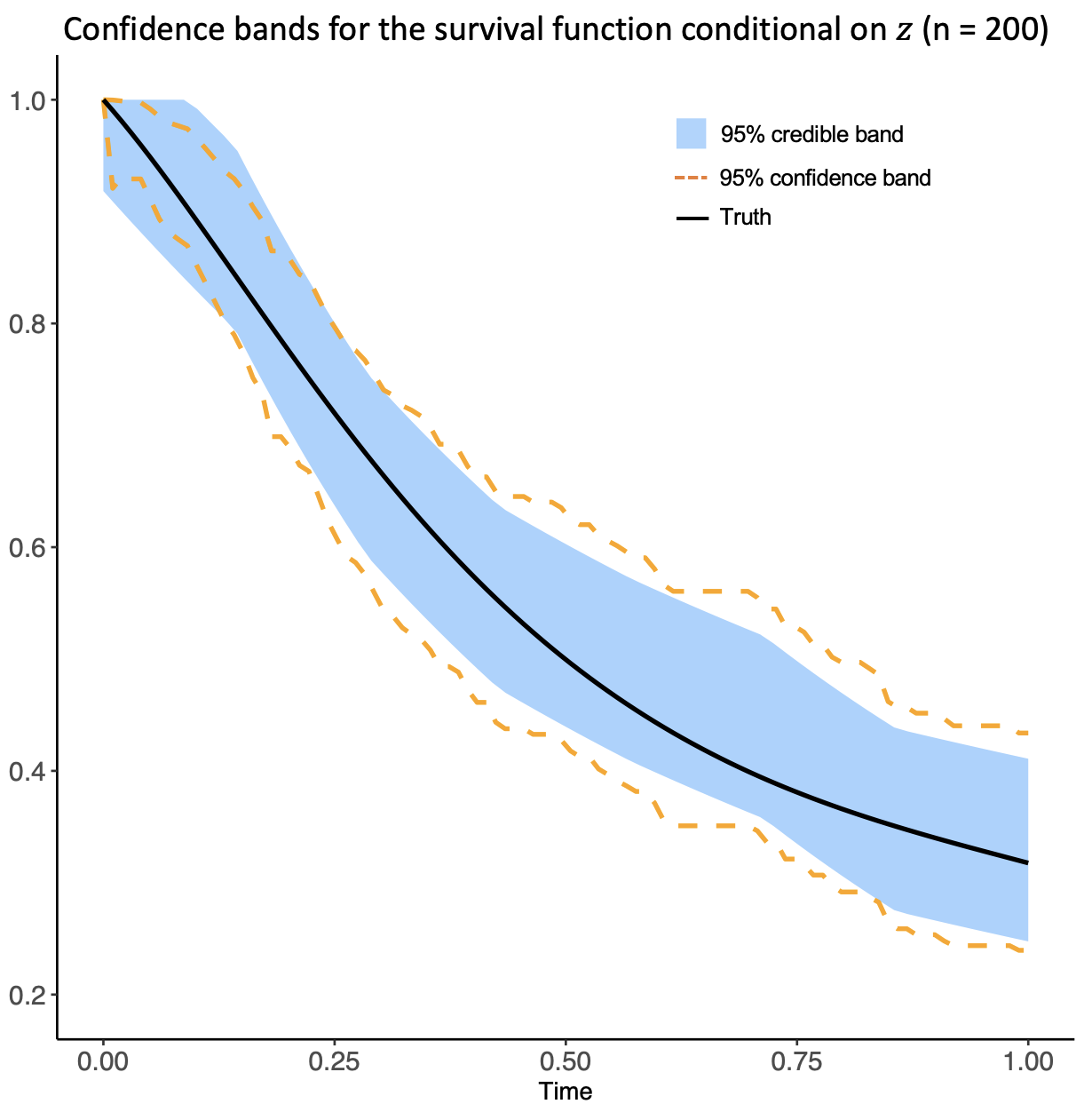
Figure 1: The 95% Bayesian credible band (blue) using the random histogram prior and the 95% frequentist confidence band (orange). The bolded black line is the true survival function conditional on $z$, $\exp\{\Lambda_{0}e^{\theta_{0}^{\prime}z}\}$. Sample size is $n=200$.

The observations from Figure 1 raise some interesting questions: can one validate and generalize our findings in the figure, that is, can one provide theory explaining why the credible band is a confidence band, and will the two bands become more similar as sample size increases? What can be said in terms of the hazard function: does the Bayesian procedure estimate it in a possibly ‘optimal’ way? We now discuss the existing literature on these questions and the main contributions of the paper.

In smooth parametric models, taking certain quantile credible sets as confidence sets is justified mathematically by the celebrated Bernstein–von Mises theorem (henceforth BvM, see e.g. van der Vaart (1998), Chapter 10): a direct consequence thereof is that taking, in dimension $1$ say, the $\alpha/2$ and $1-\alpha/2$ posterior quantiles provides a credible set (by definition) whose frequentist coverage asymptotically goes to $1-\alpha$. Its diameter also asymptotically matches the information bound so is optimal in the frequentist sense from the efficiency perspective. For more complex models, such as the Cox model, obtaining a semiparametric BvM theorem for the regression parameter is possible, as we see below, but requires non-trivial work. Obtaining analogous results at the level of the survival function itself is even more challenging. We now review recent advances in the area for such semi- and non-parametric models.

Semiparametric BvM theorems where obtained in Castillo (2012) under general conditions on the statistical model using Gaussian process priors on the nuisance parameter. Castillo and Rousseau (2015a) considered an even more general framework, allowing for BvMs for linear and non-linear functionals (also generalizing some early results of Rivoirard and Rousseau (2012) for density estimation). A multiscale approach was introduced in Castillo and Nickl (2013, 2014) in order to derive nonparametric BvM theorems for families of possibly non-conjugate priors, as well as Donsker–type theorems. Yet, the first applicative examples of these works were mostly confined to relatively simple models and/or priors.

Theory for convergence of Bayesian posterior distributions in survival models has mostly followed two directions, which we briefly review now (see also Ghosal and van der Vaart (2017), Section 12.3.3 and Chapter 13). A first series of influential results has been concerned with classes of neutral to the right priors; e.g., Hjort (1990) and Kim and Lee (2001, 2004) in the study of the standard nonparametric survival analysis model. Kim (2006) studied the Cox model, in which the joint posterior distribution of parameter and survival function was shown to satisfy the Bernstein–von Mises theorem. These results share two common features: they model the cumulative baseline hazard (equivalently, the survival function), not the baseline hazard itself—which can be desirable to model for practitioners—, and they rely on conjugacy of the class of neutral to the right priors, which provides fairly explicit characterisations of the posterior distributions.

A second series of results, closer in spirit to ours, considers priors on the baseline hazard function. De Blasi et al. (2009) used a kernel mixture with respect to a completely random measure as a prior, and obtained both posterior consistency for the hazard and limit results for linear and nonlinear functionals thereof. The work De Blasi and Hjort (2009) derived a semiparametric BvM theorem in competing risk models. The present work can be seen as following the footsteps of Castillo and van der Pas (2021a), where the simple nonparametric model with right-censoring is treated, and for which results for the hazard and cumulative hazard are derived. However, the latter model is much simpler than the Cox model, which features both regression coefficients and random covariates: this requires several more delicate bounding of both (semiparametric) bias terms and remainder terms, see Section S3 in Ning and Castillo (2023) for more details. In Castillo (2012), the Cox model is treated as an application of the general results, which yield the semiparametric BvM theorem for the Cox model parameter for (transformed) Gaussian process priors on the hazard. Although this result has a general flavor, and can be adapted to handle other prior families, it requires a fast enough posterior contraction rate for the baseline hazard, and thus cannot be applied for histogram priors on the hazard (see Section 3.1 for more on this). Perhaps more importantly, the later result is confined to the Cox regression parameter, and says nothing about uncertainty quantification for the cumulative hazard, for the survival function, or even simply for linear functionals of the hazard.

The present work obtains the first results for Bayesian uncertainty quantification jointly on regression parameters and survival function in the Cox model using non-conjugate priors. In particular, our results demonstrate that the popular and broadly used histogram priors on the baseline hazard provide not only contraction of the posterior distribution around the true unknown parameters, but also optimal and efficient uncertainty quantification on those. We adopt the multiscale analysis approach, which is motivated by Castillo and van der Pas (2021a)’s study of the survival model. More precisely, we derive

• a joint Bernstein–von Mises (BvM) theorem for linear functionals of the regression coefficients and of the baseline hazard function;

• a Bayesian Donsker theorem for the conditional cumulative hazard and survival functions;

• a minimax optimal contraction rate for the hazard function conditional on $z$ in supremum-norm distance.

We would like to highlight that (a) as well as the upper-bound part of (c) are the most important novel contributions of this paper. Given these results are proved, results (b) are obtained by adopting a similar philosophy as in Castillo and van der Pas (2021a), but still require new arguments, in particular when deriving a joint ‘nonparametric’ BvM result jointly in $(\theta,\lambda)$, see e.g. Proposition S2. The Bayesian Donsker theorem, in particular, implies that certain $(1-\alpha)\%$ credible bands for the survival function conditional on $z$ are asymptotically $(1-\alpha)\%$ confidence bands. In addition to these results, a nonparametric BvM theorem for the conditional baseline hazard function is obtained in the Supplemental Material (see Ning and Castillo, 2023). All these results are completely new for non-conjugate (in particular, histogram) priors; also, we derive the first supremum-norm posterior contraction rates for the hazard in the Cox model; we also show the corresponding matching minimax lower bound, which to the best of our knowledge was not yet available in the literature. We also demonstrate that in practice this easy-to-implementable computational algorithm can provide estimates for both the coefficients estimates and confidence bands for the cumulative hazard and survival functions. We note, as pointed out to us by a referee, that in current literature there seems to be a lack of practical algorithms in the Cox model model producing such type of bands.

Finally, the techniques we introduce have a general flavor. First, they do not rely on conjugacy of the priors considered, so that they can virtually be applied to a wide variety of families, as long as a certain change-of-measure condition is met. Second, the specific form of the model (here the Cox model) comes in through its local asymptotic normality (LAN) expansion, so similar techniques can be used in more complex settings, as long as a form of local asymptotic normality of the model holds. In particular, the techniques developed herein can serve as a useful tool for future studies of other semiparametric and nonparametric models, in survival analysis and beyond: as further discussed in Section 5.

The paper is organized as follows. Section 2 presents the model, the prior families, and key assumptions. Main results are presented in Section 3. Simulation studies are conducted in Section 4. Section 5 concludes the paper and discuss a variety extensions for future studies. All the relevant proofs for the main results and auxiliary lemmas are left to the Supplementary Material.

Notation. For any two real numbers $a$ and $b$, let $a\vee b=\max(a,b)$ and $a\wedge b=\min(a,b)$; also, let $a\lesssim b$ as $a\leq Cb$ for some constant $C$. For a positive semidefinite matrix $A$, we denote $A\succeq 0$. Let us denote by $o(1)$ a deterministic sequence going to $0$ with $n$ and $o_{P}(1)$ a sequence of random variables going to $0$ in probability under the distribution $P$. For a vector $x$, denote $\|x\|_{q}$ as the $\ell_{q}$-norm of $x$ ($q\geq 1$), i.e., $\|x\|_{q}=(\sum_{i}|x_{i}|^{q})^{1/q}$. When $q=\infty$, $\|x\|_{\infty}=\max_{i}|x_{i}|$ is the infinity norm of $x$. For a matrix $A$, denote $\|A\|_{(\infty,\infty)}=\max_{ij}|a_{ij}|$.

For a function $f\in L^{p}[a,b]$ ($p\geq 1$), where $L^{p}[a,b]$ is the space of functions whose $p$-th power is Lebesgue integrable on $[a,b]$, we define $\|f\|_{p}=(\int_{a}^{b}|f|^{p})^{1/p}$ the $L^{p}$-norm of $f$. If $p=2$, $\|f\|_{{2}}=\sqrt{\langle f,f\rangle}$ is the $L^{2}$-norm and if $p=\infty$, $\|f\|_{{\infty}}=\sup_{t}|f(t)|$ is the supremum norm. The associate inner product between any two functions, $f,g\in L^{p}[0,1]$, is denoted as $\langle f,g\rangle=\int_{0}^{1}fg$ and the space of continuous functions on $[a,b]$ is given by $\mathcal{C}[a,b]$ (resp. $L^{\infty}[a,b]$), which is equipped with the supremum norm $\|\cdot\|_{\infty}$.

For $\beta,D>0$, let $l=\lfloor\beta\rfloor$ be the largest integer smaller than $\beta$, a standard Hölder-ball on $[a,b]$ can be defined as

$$\mathcal{H}(\beta,D)=\{f:|f^{(l)}(x)-f^{(l)}(y)|\leq D|x-y|^{\beta-l},\ \|f\|_{\infty}\leq D,\ x,y\in[a,b]\}.$$

Let $(\mathcal{S},d)$ be a metric space and $\mu,\nu$ be probability measures of $\mathcal{S}$. For $F:\mathcal{S}\to\mathbb{R}$, set

$$\|F\|_{BL}=\sup_{x\in\mathcal{S}}|F(x)|+\sup_{x\neq y}\frac{|F(x)-F(y)|}{d(x,y)},$$

and denote the bounded Lipschitz metric $\mathcal{B}_{\mathcal{S}}$ as

$$\mathcal{B}_{\mathcal{S}}(\mu,\nu)=\sup_{F:\|F\|_{BL}\leq 1}\left|\int_{\mathcal{S}}F(x)(d\mu-d\nu)(x)\right|.$$

For two densities $f$ and $g$, denote $h^{2}(f,g)=\int(\sqrt{f}-\sqrt{g})^{2}d\mu$ as their squared Hellinger distance.

2 Model, prior families and structural assumptions

In this section, we first introduce the Cox model in Section 2.1. Information-related quantities of the Cox model and structural assumptions for those quantities are given in Section 2.2 and 2.3 respectively. Last, prior distributions are provided in Section 2.4.

2.1 The Cox model with random right censoring

The observations $X=X^{n}$ are $n$ independent identically distributed (i.i.d.) triplets given by $X=((Y_{1},\delta_{1},Z_{1}),\dots,(Y_{n},\delta_{n},Z_{n}))$. The observed $Y_{i}\in\mathbb{R}^{+}$ are censored versions of (unobserved) survival times $T_{i}\in\mathbb{R}^{+}$, with $\delta_{i}$ indicator variables informing on whether $T_{i}$ has been observed or not: that is, $Y_{i}=T_{i}\wedge C_{i}$ and $\delta_{i}=\mathbbm{1}(T_{i}\leq C_{i})$, where $C_{i}$’s are i.i.d. censoring times. The variables $Z_{1},\dots,Z_{n}\in\mathbb{R}^{p}$, $p$ fixed, are called covariates.

For a fixed covariate vector $z\in\mathbb{R}^{p}$ and $t>0$, define the conditional hazard rate $\lambda(t\,|\,z)=\lim_{h\to 0}h^{-1}P(t\leq T\leq t+h\,|\,T\geq t,Z=z)$. The Cox model assumes, for some $\theta\in\mathbb{R}^{p}$ and denoting by $\theta^{\prime}z$ the standard inner product in $\mathbb{R}^{p}$,

$$\lambda(t\,|\,z)=e^{\theta^{\prime}z}\lambda(t),$$

where $\lambda(t)$ is the baseline hazard function. The conditional cumulative hazard function is defined as $\Lambda(\cdot\,|\,z)=\int_{0}^{\cdot}\lambda(u\,|\,z)du=e^{\theta^{\prime}z}\int_{0}^{\cdot}\lambda(u)du=e^{\theta^{\prime}z}\Lambda(\cdot)$ and the survival function conditional on $z$ is denoted by $S(\cdot\,|\,z)=\exp(-\Lambda(\cdot\,|\,z))=\exp(-e^{\theta^{\prime}z}\Lambda(\cdot))$.

Assuming the baseline hazard rate is positive, one can alternatively make inference on the log-hazard. The unknown parameters of the Cox model are then

$$\eta=(\theta,r),\qquad\text{where }r=\log\lambda.$$

The goal is to estimate the pair $\eta=(\theta,r)$. We denote by $\eta_{0}=(\theta_{0},r_{0})$ the true values of the parameters (and similarly for the related quantities $\lambda_{0},\Lambda_{0}$).

We now give a set of standard assumptions used in this paper. First, we assume both $T$ and $Z$ admit a continuous density function, $f_{T}(\cdot)$ and $f_{Z}(\cdot)$ respectively. Given $Z$, the survival time $T$ and the censoring time $C$ are independent. At the end of the follow-up, some individuals are still event free and uncensored such that $P(T>\varrho\,|\,Z=z)>0$ and $P(C>\varrho\,|\,Z=z)=P(C=\varrho\,|\,Z=z)=0$ for some fixed time $\varrho$. The censoring $C$ is assumed to follow a distribution $G$ and admit a density such that

$$p_{C}(u)=g_{z}(u)\mathbbm{1}\{0\leq u<\varrho\}+\bar{G}_{z}(\varrho)\mathbbm{1}\{u=\varrho\}$$

with respect to $\text{Leb}([0,\varrho])+\delta_{\varrho}$, where $\text{Leb}(I)$ is the the Lebesgue measure on $I$. Without loss of generality, we assume $\varrho=1$ throughout the paper.

Based on this set-up, the joint density function of the triple $(y,\delta,z)$ is given by

$$\begin{split}f_{\eta}(y,\delta,z)=&\left(g_{z}(y)e^{-\Lambda(y)e^{\theta^{\prime}z}}\right)^{1-\delta}\left(\bar{G}_{z}(y)\lambda(y)e^{\theta^{\prime}z-\Lambda(y)e^{\theta^{\prime}z}}\right)^{\delta}f_{Z}(z)\mathbbm{1}(y<t)\\ &+\left(\bar{G}_{z}(t)e^{-\Lambda(t)e^{\theta^{\prime}z}}\right)f_{Z}(z)\mathbbm{1}(\delta=0,y=t),\end{split}$$ (1)

where $g_{z}(\cdot)$ is a continuous density of $C$ given $Z=z$, $\bar{G}_{z}(\cdot)=1-G_{z}(\cdot-)$, where $G_{z}(\cdot)$ is the cumulative distribution function of $g_{z}(\cdot)$.

Let $\ell_{n}(\eta)=\sum_{i=1}^{n}\log f_{\eta}(X_{i})$ be the log-likelihood function, the likelihood ratio is given by

$$\ell_{n}(\eta)-\ell_{n}(\eta_{0})=\sum_{i=1}^{n}\left(\delta_{i}\{(\theta-\theta_{0})^{\prime}Z_{i}+(r-r_{0})(Y_{i})\}-\Lambda(Y_{i})e^{\theta^{\prime}Z_{i}}+\Lambda_{0}(Y_{i})e^{\theta_{0}^{\prime}Z_{i}}\right).$$ (2)

From (2), one sees that the log-likelihood ratio does not depend on $g_{z}(y)$ and $\bar{G}_{z}(\cdot)$, thus one does not need to model $g_{z}(y)$ in order to make inference on $\eta$.

2.2 Information–related quantities

We now introduce some of the key quantities arising in the study of the Cox model: these are all related to the information operator (extending the usual Fisher information in parametric models) arising from the LAN–expansion in the model (see also Section 6.1). For a bounded function $b(\cdot)$ on $[0,1]$ and a cumulative hazard function $\Lambda(\cdot)$, we denote $\Lambda\{b\}(\cdot)=\int_{0}^{\cdot}b(u)d\Lambda(u)$ and, in slight abuse of notation, we set $\Lambda\{b\}=\Lambda\{b\}(1)$. The following notations are commonly used in the literature for the Cox model (see e.g., Section VIII 4.3 of Andersen et al. (1993) and Section 12.3.3 of Ghosal and van der Vaart (2017)):

$$M_{0}(u) =\mathbb{E}_{\eta_{0}}\left(e^{\theta_{0}^{\prime}Z}\mathbbm{1}_{u\leq T}\right)=\int\bar{G}_{z}(u)e^{\theta_{0}^{\prime}z-\Lambda_{0}(u)e^{\theta_{0}^{\prime}z}}f_{Z}(z)dz,$$ (3)

$$M_{1}(u) =\mathbb{E}_{\eta_{0}}\left(Ze^{\theta_{0}^{\prime}Z}\mathbbm{1}_{u\leq T}\right)=\int z\bar{G}_{z}(u)e^{\theta_{0}^{\prime}z-\Lambda_{0}(u)e^{\theta_{0}^{\prime}z}}f_{Z}(z)dz,$$ (4)

$$M_{2}(u) =\mathbb{E}_{\eta_{0}}\left(ZZ^{\prime}e^{\theta_{0}^{\prime}Z}\mathbbm{1}_{u\leq T}\right)=\int zz^{\prime}\bar{G}_{z}(u)e^{\theta_{0}^{\prime}z-\Lambda_{0}(u)e^{\theta_{0}^{\prime}z}}f_{Z}(z)dz.$$ (5)

The least favorable direction is defined as $\gamma_{M_{1}}(\cdot)=(M_{1}/M_{0})(\cdot)$. For a bounded function $b(\cdot)$ on $[0,1]$, we let $\gamma_{b}(\cdot)=(b/M_{0})(\cdot)$. The efficient information matrix of the Cox model is denoted by $\tilde{I}_{\eta_{0}}$ and is given by

$$\tilde{I}_{\eta_{0}}= \Lambda_{0}\{M_{2}(\cdot)-\gamma_{M_{1}}(\cdot)\gamma_{M_{1}}^{\prime}(\cdot)M_{0}(\cdot)\}.$$ (6)

For any $\vartheta\in\mathbb{R}^{p}$ and $g\in L^{2}\{\Lambda_{0}\}$ (i.e., $\int g^{2}d\Lambda_{0}<\infty$), we define

$$W_{n}(\vartheta,g)=\frac{1}{\sqrt{n}}\sum_{i=1}^{n}\left\{\delta_{i}\left(\vartheta^{\prime}Z_{i}+g(Y_{i})\right)-e^{\theta_{0}^{\prime}Z_{i}}\left(\vartheta^{\prime}Z_{i}\Lambda_{0}(Y_{i})+(\Lambda_{0}g)(Y_{i})\right)\right\}.$$ (7)

This quantity corresponds to the empirical process part of the LAN expansion of the Cox model (see (27) in Section 6.1 of Ning and Castillo (2023)).

2.3 Structural assumptions

The following fairly mild conditions are assumed on the unknown quantities of the model. For some positive constants $c_{1},\dots,c_{8}$,

1. the random variable $Z\in\mathbb{R}^{p}$ is bounded (i.e. $\|Z\|_{\infty}\leq c_{1}$ a.s.);

1. $\|\theta_{0}\|_{\infty}\leq c_{2}$;

Note that from (i) and (ii), one can bound $e^{\theta_{0}^{\prime}z}\leq e^{pc_{1}c_{2}}$. Also, suppose

1. $c_{3}\leq\inf_{t\in[0,\varrho]}\lambda_{0}(t)\leq\sup_{t\in[0,\varrho]}\lambda_{0}(t)\leq c_{4}$ and $r_{0}=\log\lambda_{0}\in\mathcal{H}(\beta,D)$, where $\beta,D>0$;

1. $g_{z}$ is a continuous density and $c_{5}\leq\inf_{t\in[0,\varrho]}g_{z}(t)\leq\sup_{t\in[0,\varrho]}g_{z}(t)\leq c_{6}$;

Assumptions (i)–(iv) are common in the related literature; e.g., see Castillo (2012) (p.17). As $\theta_{0},\lambda_{0},g_{z}(u)$ are all assumed to be bounded from above and below, (i)–(iv) imply

1. For $M_{2}(u)$ and $\tilde{I}_{\eta_{0}}^{-1}$ in (5) and (6) respectively, $\Lambda_{0}\{M_{2}(\cdot)\}-c_{7}I_{p}\succeq 0$ and $\|\tilde{I}_{\eta_{0}}^{-1}\|_{(\infty,\infty)}\leq c_{8}$.

The above conditions are mostly assumed for technical simplicity: boundedness of the true vector $\theta$ enables one to take a prior with bounded support, which is particularly helpful in order to carry out likelihood expansions. Attempting to remove this condition would lead to delicate questions on likelihood remainder terms and is beyond the scope of this work. The smoothness condition on the (log–) hazard is quite mild for smooth hazards: it includes for instance the case of Lipschitz hazards. Another interesting setting would be the one of piecewise constant hazards. It could be treated with the techniques developed of this paper (a given histogram can always be approximated arbitrarily well in the $L^{2}$–sense by a Haar-histogram, and then the problem becomes –nearly– parametric) although it would require a somewhat separate treatment: we refrain from providing theory here for this case, although we consider it as one of the examples of the simulations study in Section 4, where simulations show very good behavior in this setting as well. Henceforth we assume that (i)–(iv) hold without explicit reference.

2.4 Prior distributions

Priors for $\theta$ and $\lambda$ are chosen independently. The prior for $\theta$ is chosen as follows:

1. Let $\theta_{j}$ be the $j$-th coordinate of $\theta$, $\pi(\theta)=\bigotimes_{j=1}^{p}\pi(\theta_{j})=\bigotimes_{j=1}^{p}f(\theta_{j})\mathbbm{1}_{[-C,C]}$ for some constant $C>{c_{2}}$. Examples for $f(\theta_{j})$ include the uniform density, i.e., $f(\theta_{j})=1$, the truncated (to $[-C,C]$) $\tau$–Subbotin density (Subbotin, 1923), which includes the truncated Laplace (when $\tau=1$) density and truncated normal (when $\tau=2$) density as special cases.

Imposing the truncation does not seem necessary in practice, as we found in the simulation study. However, for deriving our theoretical results, and similar to Castillo (2012) and Ghosal and van der Vaart (2017), we assume that at least some upper-bound on $\|\theta\|_{\infty}$ is known, as discussed in the previous subsection (so that one can take e.g. $C=c_{2}$ in (ii)).

For the prior on $\lambda$, two classes of piecewise constant priors are considered throughout the paper:

1. Random histogram prior. For $k\geq 1,L^{\prime}=L+1$, and $L$ an $n$-dependent deterministic value to be specified below, let

   $$\lambda_{H}=\sum_{k=0}^{2^{L+1}-1}\lambda_{k}\mathbbm{1}_{I_{k}^{L+1}},$$ (8)

   where $I_{0}^{L^{\prime}}=[0,2^{-L^{\prime}}],I_{k}^{L^{\prime}}=(k2^{-L^{\prime}},(k+1)2^{-L^{\prime}}]$, and ($\lambda_{k}$) are independent random variables. We consider putting the following two types of priors on the $k$-th histogram height, $\lambda_{k}$:

• An independent Gamma prior: $\lambda_{k}\sim\text{Gamma}(\alpha_{0},\beta_{0})$ are i.i.d. variables, for some fixed positive $\alpha_{0},\beta_{0}$.

• A dependent Gamma prior: let $\lambda_{0}\sim\text{Gamma}(\alpha_{0},\beta_{0})$ and $\lambda_{k}|\lambda_{k-1}\sim\text{Gamma}(\alpha,\alpha/\lambda_{k-1})$ for some positive constant $\alpha$. Then for $k\geq 1$, $E(\lambda_{k}\,|\,\lambda_{k-1})=\lambda_{k-1}$ and $\text{Var}(\lambda_{k}\,|\,\lambda_{k-1})=\lambda_{k-1}^{2}/\alpha$.

1. Haar wavelet prior. Let $r_{S}=\log\lambda_{S}$ and again for $L$ to be specified below, let us set

   $$r_{S}=\sum_{l=-1}^{L}\sum_{k=0}^{2^{l}-1}\sigma_{l}Z_{lk}\psi_{lk},$$ (9)

   where $Z_{lk}$ are random variables, $\sigma_{l}=1$, $0\leq l\leq L$, and $(\psi_{lk})$ are Haar wavelet basis.

Although a variety of densities can be considered for $Z_{lk}$, we specifically consider for simplicity the standard normal density and the standard Laplace density (other choices of $\sigma_{l}$ e.g. $2^{-l/2}$ are possible). Note that both densities give a non-conjugate prior for $r_{S}$.

Also note that the random histogram prior can be viewed as a special case of the Haar wavelet prior if one allows for possibly dependent variables $Z_{lk}$ (and possibly different values for $\sigma_{l}$). The above priors can mostly be chosen free of dependence in the constants, except for $c_{2}$ for which we need to know at least an upper-bound for $\theta_{0}$. Such assumption is unavoidable for using bounded priors, as they put no mass outside their support.

Choice of the parameter $L$. For results on the specific priors as above, we consider the choice of cut-off $L=L_{n}$ defined as, for $\beta>0$ the assumed regularity of $r_{0}=\log\lambda_{0}$ (see (iii)),

$$2^{L_{n}}=2^{L_{n}(\beta)} \circeq\left(\frac{n}{\log{n}}\right)^{\frac{1}{2\beta+1}},$$ (10)

where $\circeq$ means that one picks a closest integer solution in $L_{n}$ of the equation. If the regularity of the true $r_{0}$ is not known in advance, as is usually the case in practice, then all the limiting shape (Bernstein–von Mises) results below go through if one replaces $\beta$ by $1/2$ in (10) (note also that all the main results, except the Hellinger rate which requires no minimal smoothness, require a regularity $\beta>1/2$). In other words, for the semiparametric results, it is enough to ‘undersmooth’. The strict knowledge of $\beta$ is only required if one wishes to obtain an optimal minimax supremum-norm contraction rate (see Section 3.4 for more on this).

3 Main results

Let us give a brief outline of our results. Section 3.1 provides a preliminary contraction result in Hellinger distance. Section 3.2 presents a joint Bernstein–von Mises (BvM) theorem for linear functionals of $\theta$ and $\lambda$. Section 3.3 derives a Donsker theorem for the joint posterior distribution of $\theta$ and the cumulative hazard function $\Lambda$. This result leads to the Donsker theorem for the posterior of the conditional cumulative hazard and survival functions. A supremum-norm convergence rate for the hazard function conditional on $z$ is obtained in Section 3.4. In Sections 3.2-3.4, we provide generic conditions that are suitable for a wide range of priors. In Section 3.5, we verify those conditions for those specific choices of priors listed in Section 2.4.

3.1 A key preliminary contraction result

We start by obtaining a preliminary Hellinger contraction rate for the posterior distribution for the priors considered above.

Define the rate, for $\beta\in(0,1]$,

$${{\nu}}_{n}={{\nu}}_{n,\beta}=\left(\frac{\log{n}}{n}\right)^{\frac{\beta}{2\beta+1}}.$$ (11)

Let $\epsilon_{n}=o(1)$ be a sequence such that $n\epsilon_{n}^{2}\to\infty$ as $n\to\infty$. Define $\zeta_{n}=\zeta_{n}(\epsilon_{n})=2^{L_{n}/2}\epsilon_{n}+2^{-\beta L_{n}}$ and

$$A_{n}=\{\eta:\ \|\theta-\theta_{0}\|\leq\epsilon_{n},\|\lambda-\lambda_{0}\|_{1}\leq\epsilon_{n},\|\lambda-\lambda_{0}\|_{\infty}\leq\zeta_{n}\}$$ (12)

Let us consider the following condition:

1. The sequences $L_{n},\epsilon_{n}$ verify $L_{n}=o(\sqrt{n}\epsilon_{n})$, $L_{n}^{2}=o(1/\epsilon_{n})$, and $\sqrt{n}\epsilon_{n}^{2}L_{n}=o(1)$ and, for $A_{n}$ as in (12),

   $$\Pi(A_{n}^{c}\,|\,X)=o_{P_{\eta_{0}}}(1).$$

Condition (P) requires the posterior distribution to contract in a certain sense around the true pair $(\theta_{0},r_{0}=\log{\lambda_{0}})$. In order to derive such a result, one may first apply the general contraction rate theorem of Ghosal et al. (2000). This, however, entails a rate for the overall density $f_{\eta}$ in the Cox model only, not the parameters themselves. The main difficulty here is then to derive results on $\theta$ and $\lambda$ separately. The rate $\epsilon_{n}$ can be thought of as a typical (possibly optimal) nonparametric rate. We call condition (P) a preliminary contraction result, because faster rates both for $\theta$ and for $\lambda$ in the supremum norm can be derived, as will be seen below. In fact, for $\theta$, it is expected that the posterior contracts at parametric, near $1/\sqrt{n}$ rate; a much more precise result is obtained in Section 3.2 below in the form of a BvM theorem.

The next lemma shows that condition (P) is indeed satisfied for the examples of priors introduced in Section 2.4.

Lemma 1.

Consider the Cox model with priors as specified in (T), and (H) or (W) with $L=L_{n}$ as in (10). Then for any $\beta\in(0,1]$ and ${{\nu}}_{n}$ as in (11),

$$\Pi[\{\eta:\ h^{2}(f_{\eta_{0}},f_{\eta})\gtrsim{{\nu}}_{n}^{2}\}\,|\,X]=o_{P_{\eta_{0}}}(1).$$

Further, for any $\beta\in(1/2,1]$, condition (P) is satisfied for these priors for $\epsilon_{n}={{\nu}}_{n}$ as in (11).

Let us now briefly comment on the preliminary supremum-norm rate $\zeta_{n}$ for $\lambda$ entailed by (P). For some cut–offs $L_{n}$, the rate can be slow. However, it is a $o(1)$ as soon as $\epsilon_{n}=o(2^{-L_{n}/2})$. For the typical choice of $L_{n}$ in (10), this only requires that $\beta>1/2$, which corresponds to a preliminary rate faster than $n^{-1/4}$. This is much less than what is required for Theorem 5 in Castillo (2012) or Theorem 12.12 in Ghosal and van der Vaart (2017), where a preliminary rate faster than $n^{-3/8}$ is needed (note that the latter rate rules out the use of regular histograms as priors, since these can get only a rate $n^{-1/3}$ at best). In Section 3.4, we show the rate $\zeta_{n}$ can be improved by adopting a multiscale analysis approach. For this, a BvM theorem for linear functionals of $\lambda$ will be needed: it is a consequence of the joint BvM derived in the next section.

From Section 3.2 to Section 3.4, we work with a generic histogram prior of the form (9) with cut–off $L=L_{n}$ (which includes both (H) and (W) as special cases), under the above condition (P). This way, the reader can directly see what generic conditions underpin our results, and adapt these to other relevant families of priors not considered here for the sake of brevity. For instance, smoother wavelet bases $(\psi_{lk})$ can be used in the prior definition and require only minor adaptations of the proofs (in a similar way as in Castillo and van der Pas (2021a) for the simple nonparametric survival model); although we do not prove this here for brevity, using these priors would enable one to derive optimal contraction rates in the supremum norm for arbitrary regularities $\beta>1/2$. We come back to the specific examples of priors (H) and (W) in Section 3.5.

3.2 The joint BvM theorem for the linear functionals of $\theta$ and $\lambda$

Let us consider the joint estimation of the two linear functionals defined by

$$\varphi_{a}(\theta)=\theta^{\prime}a,\quad\varphi_{b}(\lambda)=\langle b,\lambda\rangle=\int_{0}^{1}b(u)\lambda(u)du=\Lambda\{b\},$$ (13)

for fixed $a\in\mathbb{R}^{p}$ and $b\in L^{2}(\Lambda)$. Let us recall that we work under the generic form of prior (9) with cut–off $L=L_{n}$ and generic condition (P). Let us also recall the notation from Section 2.2: $M_{0},M_{1},M_{2}$, $\gamma_{b}(\cdot)=(b/M_{0})(\cdot)$ for a bounded function $b$, and $\tilde{I}_{\eta_{0}}$.

Consider the following conditions:

1. Let $P_{L_{n}}(\cdot)$ be the orthogonal projection onto $\mathcal{V}_{L_{n}}:=\text{Vect}\{\psi_{lk},\ l\leq L_{n},\ 0\leq k<2^{l}\}$, the subspace of $L^{2}[0,1]$ spanned by the first $L_{n}$ wavelet levels, and denote $\gamma_{b,L_{n}}=P_{L_{n}}(\gamma_{b})$ and $\gamma_{M_{1},L_{n}}=P_{L_{n}}(\gamma_{M_{1}})$. For any fixed $b\in L^{\infty}[0,1]$ and $\epsilon_{n}$ in (P),

   $$\sqrt{n}\epsilon_{n}\|\gamma_{b}-\gamma_{b,L_{n}}\|_{\infty}=o(1).$$

Condition (B) is sometimes called no-bias condition, and holds true if $b$ is sufficiently smooth and (or) the preliminary contraction rate $\epsilon_{n}$ is fast enough. Next, let $h=(t,s)\in\mathbb{R}^{2}$, for fixed $a\in\mathbb{R}^{p}$ and $b\in L^{2}(\Lambda)$, consider the two local paths:

$$\theta_{h}=\theta-\frac{t\tilde{I}_{\eta_{0}}^{-1}a}{\sqrt{n}}+\frac{s\tilde{I}_{\eta_{0}}^{-1}\Lambda_{0}\{b\gamma_{M_{1}}\}}{\sqrt{n}},$$ (14)

$$r_{h}=r+ \frac{t\gamma_{M_{1},L_{n}}^{\prime}\tilde{I}_{\eta_{0}}^{-1}a}{\sqrt{n}}-\frac{s\gamma_{b,L_{n}}}{\sqrt{n}}-\frac{s\gamma_{M_{1},L_{n}}^{\prime}\tilde{I}_{\eta_{0}}^{-1}\Lambda_{0}\{b\gamma_{M_{1}}\}}{\sqrt{n}}.$$ (15)

1. (Change of variables condition) with $r=\log\lambda$ and $r_{0}=\log\lambda_{0}$, let $\eta_{0}=(\theta_{0},r_{0})$ and $\eta_{h}=(\theta_{h},r_{h})$, where $\theta_{h}$ in (14) and $r_{h}$ in (15) with $a,b$ to be specified below and $A_{n}$ as in (P), suppose

   $$\frac{\int_{A_{n}}e^{\ell_{n}(\eta_{h})-\ell_{n}(\eta_{0})}d\Pi(\eta)}{\int e^{\ell_{n}(\eta)-\ell_{n}(\eta_{0})}d\Pi(\eta)}=1+o_{P_{\eta_{0}}}(1).$$

Condition (C1) is often called change of variables condition: indeed, one natural way to check it is via controlling the change in distribution from $\eta\sim\Pi$, to the distribution induced on $\eta_{h}$. For priors such as (H) and (W), this can be checked by posing a change of variables with respect to the Lebesgue measure on $\mathbb{R}^{L_{n}}$. The verification of these conditions for these priors is given in Section S7.2.

For $\eta\sim\Pi(\cdot\,|\,X)$, $\mu=(\mu_{1},\mu_{2})\in\mathbb{R}^{2}$, $a\in\mathbb{R}^{p}$, and $b\in L^{2}(\Lambda)$, let us define the map

$$\tau_{\mu}:\eta\to\sqrt{n}(\theta^{\prime}a-\mu_{1},\langle\lambda,b\rangle-\mu_{2}),$$

and let $\Pi(\cdot\,|\,X)\circ\tau_{\mu}^{-1}$ be the distribution induced on $\sqrt{n}(\theta^{\prime}a-\mu_{1},\langle\lambda,b\rangle-\mu_{2})$. We are ready to present the joint BvM theorem for the bivariate functions $\varphi_{a}(\theta)$ and $\varphi_{b}(\lambda)$.

Theorem 1.

Let $a$ and $b$ be fixed elements of $\mathbb{R}^{p}$ and $L^{2}(\Lambda_{0})$ respectively, for any $b$ that satisfies (B), suppose the prior for $\eta=(\theta,\lambda)$ is chosen such that (P) and (C1) hold. Then

$$\mathcal{B}_{\mathbb{R}^{2}}\left(\Pi(\cdot\,|\,X)\circ\tau_{\hat{\varphi}}^{-1},\mathcal{L}(a^{\prime}\mathbb{V},\Upsilon_{b}-\mathbb{V}\Lambda_{0}\{b\gamma_{M_{1}}\})\right)\stackrel{{\scriptstyle P_{\eta_{0}}}}{{\to}}0,$$ (16)

where $\mathbb{V}$ and $\Upsilon_{b}$ are independent, $\mathbb{V}\sim N\left(0,\tilde{I}_{\eta_{0}}^{-1}\right)$ and $\Upsilon_{b}\sim N(0,\Lambda_{0}\{b\gamma_{b}\})$, $\mathcal{B}_{\mathbb{R}^{2}}$ is the bounded Lipschitz metric between distributions on $\mathbb{R}^{2}$, and $\hat{\varphi}=(\hat{\varphi}_{a}(\theta),\hat{\varphi}_{b}(\lambda))$ is given by

$$\hat{\varphi}_{a}(\theta) :=\varphi_{a}(\hat{\theta})=\varphi_{a}(\theta_{0})+\frac{1}{\sqrt{n}}W_{n}\left(\tilde{I}_{\eta_{0}}^{-1}a,\ -\gamma_{M_{1}}^{\prime}\tilde{I}_{\eta_{0}}^{-1}a\right),$$

$$\hat{\varphi}_{b}(\lambda):=\varphi_{b}(\hat{\lambda}) =\varphi_{b}(\lambda_{0})+\frac{1}{\sqrt{n}}W_{n}\left(-\tilde{I}_{\eta_{0}}^{-1}\Lambda_{0}\{b\gamma_{M_{1}}\},\gamma_{b}+\gamma_{M_{1}}^{\prime}\tilde{I}_{\eta_{0}}^{-1}\Lambda_{0}\{b\gamma_{M_{1}}\}\right).$$

The centering sequences in the last display of the statement can be seen to be ‘efficient’ ones from the semiparametric perspective (see e.g. van der Vaart (1998), Chapter 25). An important added value to the joint BvM (in contrast to individual limiting statement for marginal coordinates) is that it captures the dependence between $\theta$ and $\lambda$: a practical application is given in Figure 4. The result enables to consider many combinations of functionals by choosing specific $a\in\mathbb{R}^{p}$ and $b\in L^{2}(\Lambda_{0})$. For example, let $a=(1,0,\dots,0)$ and $b=\mathbbm{1}_{[0,1]}$: Theorem 1 implies a joint joint BvM for $(\theta_{1},\Lambda(1))$, where $\theta_{1}$ is the first coordinate of $\theta$ and $\Lambda(1)=\int_{0}^{1}\lambda$ is the cumulative hazard function at time one. The limiting distribution is given in the next corollary, where, in addition, we center the joint posterior at efficient frequentist estimators for $\theta$ and $\Lambda(1)$.

Corollary 1 (Joint BvM for $\theta_{1}$ and $\Lambda(1)$).

Consider the Cox model with the density function in (1), let $a=(1,0,\dots,0)$ and $b=1$, and $\tau_{(\hat{\theta}_{1},\hat{\Lambda}(1))}$ be the map such that

$$\tau_{(\hat{\theta}_{1},\hat{\Lambda}(1))}:\eta\rightarrow\sqrt{n}\left(\theta_{1}-\hat{\theta}_{1},\Lambda(1)-\hat{\Lambda}(1)\right),$$

where $\hat{\theta}$ is the maximum Cox partial likelihood estimator and $\hat{\Lambda}(1)$ is the Breslow estimator. Denote $\Pi(\cdot\,|\,X)\circ\tau_{(\hat{\theta}_{1},\hat{\Lambda}(1))}^{-1}$ as the distribution induced on $\sqrt{n}(\theta_{1}-\hat{\theta}_{1},\Lambda(1)-\hat{\Lambda}(1))$, then under the same conditions as in Theorem 1,

$$\mathcal{B}_{\mathbb{R}^{2}}\left(\Pi(\cdot\,|\,X)\circ\tau_{(\hat{\theta}_{1},\hat{\Lambda}(1))}^{-1},\ \mathcal{L}(a^{\prime}\mathbb{V},\Upsilon_{1}-\mathbb{V}\Lambda_{0}\{\gamma_{M_{1}}\})\right)\stackrel{{\scriptstyle P_{\eta_{0}}}}{{\to}}0,$$ (17)

where $\Upsilon_{1}\sim N(0,\Lambda_{0}\{M_{0}^{-1}\})$ and $\mathbb{V}\sim N(0,\tilde{I}_{\eta_{0}}^{-1})$ are independent.

An immediate practical implication of the BvM theorem in Corollary 1 is that two-sided quantile credible sets for $\hat{\theta}_{1}$ (or more generally for any given coordinate $\theta_{j}$, $j=1,\dots,p$) are asymptotically optimal confidence sets from the perspective. Results in this vein can also be derived for the survival function in the functional sense: this is the object of the next section.

3.3 Joint Bayesian Donsker theorems

We now present the second main result in this paper, the Bayesian Donsker theorem for the joint posterior distribution of $\theta$ and the cumulative hazard function $\Lambda(\cdot)$.

Let us denote

$$W_{n}^{(1)}=W_{n}^{\star}\left(\tilde{I}_{\eta_{0}}^{-1},\ -\gamma_{M_{1}}^{\prime}\tilde{I}_{\eta_{0}}^{-1}\right),$$ (18)

where $W_{n}^{(1)}$ is a $p$-dimensional vector and

$$\begin{split}W_{n}^{\star}\left(\tilde{I}_{\eta_{0}}^{-1},\ -\gamma_{M_{1}}^{\prime}\tilde{I}_{\eta_{0}}^{-1}\right)=\frac{1}{\sqrt{n}}\sum_{i=1}^{n}\left\{\delta_{i}\tilde{I}_{\eta_{0}}^{-1}\left(Z_{i}-\gamma_{M_{1}}\right)-e^{\theta_{0}^{\prime}Z_{i}}\tilde{I}_{\eta_{0}}^{-1}\left(Z_{i}\Lambda_{0}(Y_{i})-(\Lambda_{0}{\gamma_{M_{1}}})(Y_{i})\right)\right\},\end{split}$$

and given $b\in L^{2}(\Lambda_{0})$,

$$W_{n}^{(2)}(b)=W_{n}\left(-\tilde{I}_{\eta_{0}}^{-1}\Lambda_{0}\{b\gamma_{M_{1}}\},\gamma_{b}+\gamma_{M_{1}}^{\prime}\tilde{I}_{\eta_{0}}^{-1}\Lambda_{0}\{b\gamma_{M_{1}}\}\right).$$ (19)

Define the centering sequences for $\theta$ and $\lambda$ as follows:

$$T_{n}^{\theta}=\theta_{0}+W_{n}^{(1)}/\sqrt{n},$$

and, for a given sequence $L_{n}$,

$$\langle T_{n}^{\lambda},\psi_{lk}\rangle=\begin{cases}\langle\lambda_{0},\psi_{lk}\rangle+W_{n}^{(2)}(\psi_{lk})/\sqrt{n}&\quad\text{if}\ l\leq L_{n},\\ \ 0&\quad\text{if}\ l>L_{n}.\end{cases}$$

The Donsker theorem requires, in addition to (C1), a similar condition, where $t$ and $s$ are allowed to increase with $n$. This condition is stated as follows:

1. (Change of variables condition, version 2) with the same notation as in (C1), let $\eta_{h}=(\theta_{h},r_{h})$, $\theta_{h}$ and $r_{h}$ be the local paths in (14) and (15) respectively with $a,b$ to be specified below, for $n$ large enough and any $|t|,|s|\leq\log n$, one assumes, for $A_{n}$ as in (P) and some constant $C_{1}>0$,

   $$\frac{\int_{A_{n}}e^{\ell_{n}(\eta_{h})-\ell_{n}(\eta_{0})}d\Pi(\eta)}{\int e^{\ell_{n}(\eta)-\ell_{n}(\eta_{0})}d\Pi(\eta)}\leq e^{C_{1}(1+t^{2}+s^{2})}.$$

Condition (C2) is similar to (C1). A major difference between the two conditions is that in (C2), $t$ and $s$ are allowed to increase with $n$; however, in (C1), $t$ and $s$ are fixed.

We further require the rates $\epsilon_{n}$ and $\zeta_{n}$ and the cut-off $L_{n}$ in (P) to satisfy

$$\sqrt{n}\epsilon_{n}2^{-L_{n}}=o(L_{n}^{-5/2}),\quad\zeta_{n}L_{n}^{2}=o(1),$$ (20)

Theorem 2 (Joint Bayesian Donsker theorem).

Suppose the prior for $\eta=(\theta,\eta)$ is chosen such that both (P) and (20) hold. Suppose (C1) holds for $a=z$, any fixed $z\in\mathbb{R}^{p}$, and any $b\in\mathcal{V}_{\mathcal{L}}=\text{Vect}\{\psi_{lk},\ l\leq L_{n},\ 0\leq k<2^{l}\}$ for a fixed $\mathcal{L}$ and (C2) holds uniformly for $a=z$, any fixed $z\in\mathbb{R}^{p}$, and any $b=\psi_{LK}$ with $0\leq L\leq L_{n}$ and $0\leq K<2^{L}$.

Let $\mathcal{L}((\theta,\Lambda(\cdot))\in\cdot\,|\,X)$ be the distribution induced on $\theta$ and $\Lambda(\cdot)=\int_{0}^{\cdot}\lambda$ and $\mathbb{T}_{n}^{\lambda}(\cdot)=\int_{0}^{\cdot}T_{n}^{\lambda}$ be the centering for $\Lambda(\cdot)$. Denote $\mathbb{B}(\cdot)$ as standard Brownian motion and set $U_{0}(\cdot)=\int_{0}^{\cdot}(\lambda_{0}/M_{0})(u)du$. Let $\mathbb{V}\sim N(0,\tilde{I}_{\eta_{0}}^{-1})$ that is independent of $\mathbb{B}(\cdot)$. Then, as $n\to\infty$,

$$\mathcal{B}_{\mathbb{R}^{p}\times\mathcal{C}([0,1])}\left(\mathcal{L}\left(\sqrt{n}(\theta-T_{n}^{\theta},\Lambda(\cdot)-\mathbb{T}_{n}^{\lambda}(\cdot))\,|\,X\right),\ \mathcal{L}\left(\mathbb{V},\mathbb{B}(U_{0}(\cdot))-\mathbb{V}^{\prime}\Lambda_{0}\{\gamma_{M_{1}}\}(\cdot)\right)\right)\stackrel{{\scriptstyle P_{\eta_{0}}}}{{\to}}0,$$ (21)

where $\mathcal{B}_{\mathbb{R}^{p}\times\mathcal{C}([0,1])}$ is the bounded-Lipschitz metric on $\mathbb{R}^{p}\times\mathcal{C}([0,1])$.

Remark 1.

While the proof is left to the supplemental material (Ning and Castillo, 2023), a key step for obtaining the joint Bayesian Donsker theorem, following ideas from Castillo and Nickl (2014), is to establish first a BvM for $(\theta,\lambda)$ in an appropriate space. However, unlike in Castillo and Nickl (2014) where one can work directly on the nonparametric quantity of interest, here due to the split semiparametric model at hand, one needs to prove a joint nonparametric BvM for the pair $(\theta,\lambda)$, see Proposition S2. This result is new in this context and is of independent interest for proving similar results in other semiparametric models.

The centerings $T_{n}^{\theta}$ and $\mathbb{T}_{n}^{\lambda}$ in Theorem 2 can be replaced with any efficient estimators for $\theta$ and $\Lambda$: the next corollary formalizes this with centering at standard frequentist estimators.

Corollary 2.

Let $\hat{\theta}$ be the maximum Cox partial likelihood estimator and $\hat{\Lambda}(\cdot)$ be the Breslow estimator, then, under the same conditions as in Theorem 2, as $n\to\infty$,

$$\mathcal{B}_{\mathbb{R}^{p}\times\mathcal{D}([0,1])}\left(\mathcal{L}\left(\sqrt{n}(\theta-\hat{\theta},\Lambda(\cdot)-\hat{\Lambda}(\cdot))\,|\,X\right),\ \mathcal{L}\left(\mathbb{V},\mathbb{B}(U_{0}(\cdot))-\mathbb{V}^{\prime}\Lambda_{0}\{\gamma_{M_{1}}\}(\cdot)\right)\right)\stackrel{{\scriptstyle P_{\eta_{0}}}}{{\to}}0,$$ (22)

where $\mathcal{D}([0,1])$ is the Skorokhod space on $[0,1]$.

Corollary 2 immediately implies the Bernstein-von Mises theorem for the marginal posterior distribution of $\theta$: $\mathcal{B}_{\mathbb{R}^{p}}\left(\mathcal{L}(\sqrt{n}(\theta-\hat{\theta})\,|\,X),\mathbb{V}\right)\stackrel{{\scriptstyle P_{\eta_{0}}}}{{\to}}0$. As an application of Corollary 2, one obtains the Bayesian Donsker theorem for the conditional hazard and survival functions by simply applying the functional delta method (Chapter 20 in van der Vaart, 1998). Let $z$ be a fixed element in $\mathbb{R}^{p}$, and recall we define $S(\cdot\,|\,z)=\exp(-\Lambda(\cdot)e^{\theta^{\prime}z})$, the survival function conditional on $z$. Denote $\hat{S}(\cdot\,|\,z)=\exp(-\hat{\Lambda}(\cdot)e^{\hat{\theta}^{\prime}z})$ with $\hat{\theta}$ and $\hat{\Lambda}(\cdot)$ the frequentist estimators as above, then, as $n\to\infty$,

$$\mathcal{B}_{\mathcal{D}([0,1])}\left(\mathcal{L}\left(\sqrt{n}(\Lambda(\cdot)e^{\theta^{\prime}z}-\hat{\Lambda}(\cdot)e^{\hat{\theta}^{\prime}z})\,|\,X\right),\ \mathcal{L}(\mathbb{H}_{1})\right)\stackrel{{\scriptstyle P_{\eta_{0}}}}{{\to}}0,$$ (23)

$$\mathcal{B}_{\mathcal{D}([0,1])}\left(\mathcal{L}\left(\sqrt{n}(S(\cdot\,|\,z)-\hat{S}(\cdot\,|\,z))\,|\,X\right),\ \mathcal{L}(\mathbb{H}_{2})\right)\stackrel{{\scriptstyle P_{\eta_{0}}}}{{\to}}0,$$ (24)

where $\mathbb{H}_{1}$ and $\mathbb{H}_{2}$ are the transformed processes obtained after applying the functional delta method from (22). Moreover, by applying the continuous mapping theorem and noting that the map for any function $f\to\|f\|_{\infty}$ is continuous from $\mathcal{D}([0,1])$, equipped with the supremum norm, to $\mathbb{R}^{+}$, (23) and (24) imply

$$\mathcal{B}_{\mathbb{R}}\left(\mathcal{L}\left(\sqrt{n}\|\Lambda(\cdot)e^{\theta^{\prime}z}-\hat{\Lambda}(\cdot)e^{\hat{\theta}^{\prime}z}\|_{\infty}\,|\,X\right),\ \mathcal{L}\left(\|\mathbb{H}_{1}\|_{\infty}\right)\right)\stackrel{{\scriptstyle P_{\eta_{0}}}}{{\to}}0,$$

$$\mathcal{B}_{\mathbb{R}}\left(\mathcal{L}\left(\sqrt{n}\|S(\cdot\,|\,z)-\hat{S}(\cdot\,|\,z)\|_{\infty}\,|\,X\right),\ \mathcal{L}\left(\|\mathbb{H}_{2}\|_{\infty}\right)\right)\stackrel{{\scriptstyle P_{\eta_{0}}}}{{\to}}0.$$

A simple consequence of the last display is that the two-sided $(1-\alpha)\%$ quantile credible band for the conditional hazard (resp. the survival function conditional on $z$) function is asymptotically a two-sided $(1-\alpha)\%$ confidence band (see Castillo and Nickl (2014), Corollary 2).

3.4 The supremum-norm convergence rate for the hazard function conditional on $z$

In this section, we present the third main result: a faster supremum-norm posterior contraction rate for the hazard function conditional on $z$ than the rate $\zeta_{n}$ in (P). We denote this rate as $\xi_{n}$, which depends on $L_{n}$, a diverging sequence, such that $L_{n}2^{L_{n}}\lesssim\sqrt{n}$, where

$$\xi_{n}:=\xi_{n}(\beta,L_{n},\epsilon_{n})=\sqrt{\frac{L_{n}2^{L_{n}}}{n}}+2^{-\beta L_{n}}+\epsilon_{n}.$$

Theorem 3.

Suppose $r_{0}\in\mathcal{H}(\beta,D)$ with $1/2<\beta\leq 1$. Let $L_{n}$ be a diverging sequence such that $L_{n}2^{L_{n}}\lesssim\sqrt{n}$ and let $z\in\mathbb{R}^{p}$ be fixed. For the prior of $\eta=(\theta,\lambda)$ chosen such that both (P) and (20) hold, and (C2) also holds uniformly for $a=z$ and any $b=\psi_{LK}$, with $(\psi_{LK})$ the Haar wavelet basis, $0\leq L\leq L_{n}$ and $0\leq K<2^{L}$, then for $\xi_{n}=o(1)$ and $n\xi_{n}^{2}\to\infty$, and an arbitrary sequence $M_{n}\to\infty$,

$$\Pi\left(\eta:\|\lambda e^{\theta^{\prime}z}-\lambda_{0}e^{\theta_{0}^{\prime}z}\|_{\infty}>M_{n}\xi_{n}\,|\,X\right)=o_{P_{\eta_{0}}}(1).$$ (25)

We will show that in the next section, with a specific choice of the value of $L_{n}$, the rate $\xi_{n}$ is within the same order of the Hellinger rate ${{\nu}}_{n}$ in (11).

3.5 Results for specific priors

In this section, we apply the generic results in Sections 3.2, 3.3, and 3.4 to study the specific priors considered in Section 2.4. The result is stated in the following theorem.

Theorem 4.

Consider the Cox model with the priors as specified in (T), and (H) or (W) with $L=L_{n}$ in (10) and ${{\nu}}_{n}$ given in (11). For any $\beta\in(1/2,1]$,

1. conditions (P) and (C1) hold, (B) holds for any $b\in\mathcal{H}(\mu,D)$ with $\mu>1/2$ and $D>0$, then, (16) in Theorem 1 holds;

2. condition (C2) also holds, thus (21) in Theorem 2 holds;

3. the supremum-norm rate $\xi_{n}$ in (25) can be taken to be $\xi_{n}={{\nu}}_{n}$ as in (11).

The proof of this result, implying that conditions (P), (B), (C1), and (C2) hold for priors given in Section 2.4, can be found in Ning and Castillo (2023).

Remark 2.

If $\beta>1$, the first and second points in Theorem 4 still hold. The third point also holds but the supremum-norm rate becomes $(\log n/n)^{1/3}$.

Let us compare the supremum rate ${{\nu}}_{n}$ in the third point of the theorem and the rate $\zeta_{n}$ obtained in Lemma 1. Obviously, ${{\nu}}_{n}<\zeta_{n}$, as $\zeta_{n}\geq 2^{L_{n}/2}{{\nu}}_{n}$, and $L_{n}\to\infty$ as $n\to\infty$. In fact, by plugging-in the value of $L_{n}$ in (10), one obtains $\zeta_{n}=(\log n/n)^{\frac{2\beta-1}{2(2\beta+1)}}$ which can become extremely slow when $\beta$ is close to $1/2$. In Lemma S17 in Ning and Castillo (2023), we derive a lower bound for the minimax rate in the supremum norm for the hazard which shows that the rate ${{\nu}}_{n}$ is sharp. To our best knowledge, this is the first sharp supremum-norm result for the hazard obtained for the Cox model.

The cut-off $L_{n}$ in our theorems is chosen to be a deterministic sequence depending on $n$ and the smoothness level $\beta$. As noted below (10), for semiparametric-type results, including Donsker theorems, it is enough to ‘undersmooth’, and all such results hold for a smoothness parameter taken to be $1/2$ in (10) whenever the true smoothness $\beta$ is larger than 1/2, and this choice already provides a contraction rate of $n^{-1/4}$ for the posterior of the conditional hazard. It is natural to ask whether the cut-off parameter $L$ can itself be taken random in a hierarchical Bayes approach. Although often used in practice too, we underline that particular caution must be taken with such an ‘adaptive’ prior: indeed, as demonstrated in Castillo and Rousseau (2015a) (Section 4.3) in the density estimation model, BvM results may fail to hold for such a prior. This phenomenon would appear in the Cox model too if the regularities of the hazard and of the least favorable direction are too far apart. Regarding adaptive supremum norm rate (or nonparametric BvM) results, it is conceivable that spike-and-slab type priors would work, as in Ray (2017), although unlike in the white noise setting considered in Ray (2017), one could not use conjugacy here, so this is beyond of the scope of this paper and left for future investigation.

4 Simulation studies

Two simulation studies are conducted in this section. The first study, described in Section 4.2, compares the limiting distribution given in Corollary 1 with the empirical distributions obtained from the MCMC algorithm, which is given in Section 4.1. The second study compares the coverage and the area of the 95% credible bands for the MCMC algorithm to the 95% confidence bands for a commonly used frequentist method by varying the sample size and changing the censoring distribution. We choose the two random histogram priors for $\lambda$ as given in Section 2.4. The prior for $\theta$ is chosen as the standard normal distribution. If $\theta$ is multivariate, we use the standard multivariate normal density instead. In Section 4.1, we describe how we generate the simulated data and the MCMC sampler. Section 4.2 presents results for the first study, and Section 4.3 summarizes results for the second study.

4.1 Generating the data and the MCMC sampler

The data are generated from the “true” conditional hazard function $\lambda_{0}(t)e^{\theta_{0}^{\prime}z}$, where $\lambda_{0}$ and $\theta_{0}$ will be specified below. The “observations” $X^{n}=(Y^{n},\delta^{n})$ are generated using the “simsurv” function in $\mathsf{R}$ (Brilleman et al., 2020). We consider the following two types of censoring:

1. Administrative censoring only. Time points are censored at a fixed time point $t=1$;

2. Administrative censoring $+$ uniform censoring. The censoring time is generated from the uniform distribution on $[0,1]$. Any time point beyond $t=1$ is also censored.

Although the first type of censoring violates our assumption in Section 2.3, as we assumed the censoring follows a random distribution, it is interesting to find out in the next two sections that the empirical results still match with our theoretical results quite well.

Posterior draws are obtained using the MCMC algorithm given as follows:

1. For the independent gamma prior, since it is conjugate with the posterior distribution given $\theta$, we sample each $\lambda_{k}\sim\text{Gamma}(d_{k}+\alpha,T_{k}(\theta)+\beta)$, where $d_{k}=\sum_{i=1}^{n}\delta_{ki}$ is the number of events in $k$-th interval and $T_{k}(\theta)=\sum_{i=1}^{n}Y_{ik}e^{\theta Z_{i}}$, $\alpha$ and $\beta$ are the hyperparameters, and we chose them to 1. After obtaining samples for $(\lambda_{lk})$, we draw $\theta$. Since $\pi(\theta)$ is not conjugate, we first draw a candidate from the proposal density, i.e., $\theta^{\text{prop}}\sim N(\theta^{\text{prev}},1)$, where $\theta^{\text{prev}}$ stands for the draw from the previous iteration, and then use the Metropolis algorithm to accept or reject this candidate.

2. For the dependent gamma prior, as it is non-conjugate, we thus draw each $\lambda_{k}$ from the proposal density as follows: $\lambda_{1}^{\text{prop}}\sim\text{Gamma}(d_{1}+\alpha_{0}-\alpha,\ T_{1}(\theta)+\beta_{0})$ and $\lambda_{k}^{\text{prop}}\sim\text{Gamma}(d_{k}+\varepsilon,\ \alpha/\lambda_{k-1}+T_{k}(\theta))$ for $k=2,\dots,L_{n}-1$. The last interval $\lambda_{K}\sim\text{Gamma}(d_{K}+\alpha,\ \alpha\lambda_{K-1}+T_{K}(\theta))$ for $K=L_{n}$. In practice, we choose $\varepsilon=10^{-6}$, $\alpha_{0}=1.5$ and $\alpha=\beta_{0}=1$. The proposal density for $\theta$ is the same.

To initialize the MCMC algorithm, we choose the initial values for $\theta$ and $\lambda_{k}$ as their frequentist estimators (the same as in Corollary 2). We choose $L_{n}$ as in (10) and $\beta=1/2$. For each simulation, we run 10,000 iterations and discard the first 2,000 draws as burn-in.

Let us now discuss in more detail the simulation in Figure 1. The dataset is generated by choosing $\theta_{0}=-0.5$ and $\lambda_{0}(t)=6\times((t+0.05)^{3}-2(t+0.05)^{2}+t+0.05)+0.7,\ t\in[0,1]$. We generate the covariate $z$ randomly from the standard normal distribution. Here, the true function $\lambda_{0}$ is chosen the same as it in the simulation of Castillo and van der Pas (2021a); see also in their $\mathsf{R}$ package ‘BayesSurvival’ (van der Pas and Castillo, 2021). However, this choice is for illustration purposes and otherwise fairly arbitrary. Similar simulation results would hold if choosing other either smoothly varying or piecewise constant functions (see Section 4.3, which we chose different $\theta_{0}$ and $\lambda_{0}$). We note once again that, although our theoretical results assume Hölder smoothness of the true log-hazard, the techniques go through for histogram true hazards as well). In Figure 1, only administrative censoring is considered. The prior is chosen to be the independent gamma prior (choosing the dependent gamma prior won’t change the result dramatically, as can be seen in Table 1 below). The 95% credible band is a fixed width band whose width is constant with the time. The width is determined such that the posterior probability is 95%. The 95% confidence band, on the other hand, is obtained using the $\mathsf{predictCox}$ function of the ‘riskRegression’ package in $\mathsf{R}$ (Gerds and Kattan, 2021). Its width varies with time.

Here we briefly describe the approach used in their package. We refer the interested readers to read Lin et al. (1994) and Scheike and Zhang (2008) for more details. Using the fact that the frequentist estimator $(\hat{\theta},\hat{\Lambda})$ converges to the same limiting process as the joint distribution $(W_{n}^{(1)},\int_{0}^{t}W_{n}^{(2)}(\mathbbm{1}_{u\leq t})du)$, where $W_{n}^{(1)}$ and $W_{n}^{(2)}$ are given in (18) and (19), their approach first defines another process, depending on $W_{n}^{(1)}$ and $W_{n}^{(2)}$, that is asymptotically equivalent to $\sqrt{n}\left(\hat{\Lambda}(t)e^{\hat{\theta}^{\prime}z}-\Lambda(t)e^{\theta^{\prime}z}\right)$; see equation 2.1 in Lin et al. (1994) for the exact expression of that process. Their approach then further approximates that process by a summation of independent normal variables whose distribution can be easily generated through Monte Carlo simulation and replaces other unknown quantities with their sample estimators. After large enough samples are generated, the last step is to obtain the size of the 95% confidence band for the conditional cumulative hazard function by choosing the 95th quantile from those samples. The confidence band for the survival function conditional on $z$ can be obtained similarly, except that one first needs to apply the functional delta method to obtain the limiting process for the survival function conditional on $z$. The remaining parts are the same.

4.2 Study I: Comparing the empirical posterior distributions and the limiting distributions of $\theta$ and $\Lambda(1)$

We compare the limiting distribution given in Corollary 1 with the empirical distribution obtained using the MCMC sampler in Section 4.1. We will study the joint posterior distribution of $\theta$ and $\lambda$. For simplicity, we let $\theta_{0}=-0.5$ (for now, we simply choose it to be univariate; simulation results for using a multivariate $\theta$ are given in the next section) and generate the covariate $z$ randomly from the standard normal distribution. We also choose $\lambda_{0}(t)=6\times((t+0.05)^{3}-2(t+0.05)^{2}+t+0.05)+0.7,\ t\in[0,1]$ and generate the hazard rate with a sample of 1,000. We choose the prior for $\theta$ as the standard normal distribution and the prior for $\lambda$ as the independent gamma prior. Results for choosing the dependent gamma prior are similar. To obtain draws, we run the MCMC algorithms in parallel for 1,000 times. Each time we only record the last pair draw for $\theta$ and $\Lambda(1)$, where $\Lambda(1)=\sum_{k=1}^{L_{n}}\lambda_{k}$. Therefore, the 1,000 draws we obtained are independent.

We first study the marginal posterior distributions for $\theta$ and $\Lambda(1)$. In Figures 3 and 3, we first draw their empirical histogram from the 1,000 independent draws. We then draw a normal density with blue color centered at the posterior mean, and its variance is estimated from those draws. Last, we draw another normal density with red color, which has the same centering as the blue one, but its variance is chosen as the theoretical value from the limiting distribution in Corollary 1. We observe that in either the left plot (i.e., for $\theta$) or the right plot (i.e., for $\Lambda(1)$), the density with blue color is well aligned with the one with red color. This finding suggests that empirical variances are close to their theoretical variances obtained from the corollary. We also found that both empirical histograms show similar shapes as their corresponding normal density, which verifies their limiting distributions should be normal. Last, both the true values of $\theta_{0}$ and $\Lambda_{0}(1)$, $-0.5$ and $1.2$ respectively, are contained inside the corresponding 95% credible intervals. For $\theta$, the interval is $[-0.54,-0.39]$, and for $\Lambda(1)$, it is $[1.14,1.34]$.

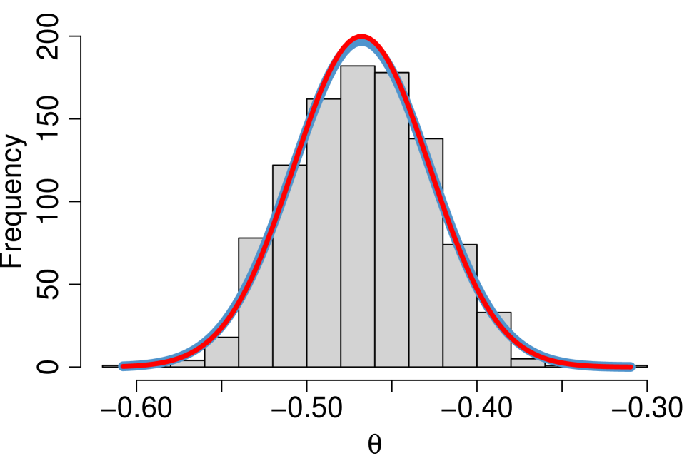
Figure 2: Plot of the empirical histogram, the empirical distribution (blue), and the limiting distribution (red) for the marginal posterior distribution of $\theta$. True value of $\theta$ is $-0.5$.

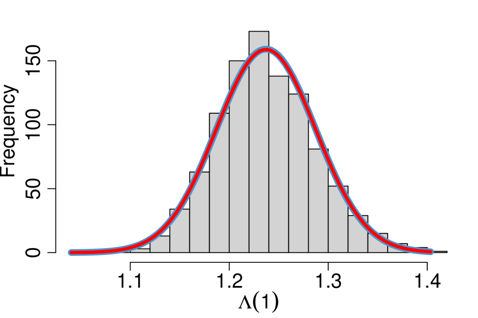
Figure 3: Plot of the empirical histogram, the empirical distribution (blue), and the limiting distribution (red) for the marginal posterior distribution of $\Lambda(1)$. True value of $\Lambda(1)$ is $1.2$.

Next, we study the joint posterior distribution of $\theta$ and $\Lambda(1)$, which involves the correlation between the two quantities. In Figure 4, we give three plots. In (a), we plot the 86%, 90%, 95%, and 99% contour plots of the limiting joint distribution in Corollary 1. In (b), we plot the contours with the same four quantiles for a bivariate normal distribution, which its mean, variances, and correlations are estimated from the 1,000 draws. In (c), we found that the two sets of contour plots in (a) and (b) indeed align quite well, which suggests that the empirical distribution matches with the theoretical limiting distribution in the corollary. Our calculation reveals that the correlation between $\theta$ and $\Lambda(1)$ in (a) is 0.15 and that in (b) is 0.10. A benefit of studying the joint posterior distribution with the correlation is that one can obtain the elliptical credible sets instead of rectangular credible sets. The length and the width of the rectangular credible sets are the 97.5% credible intervals of $\theta$ and $\Lambda(1)$ respectively. Therefore, the area of a rectangular credible set is typically larger than that of an elliptical credible set. For example, in (b), the area of the 95% elliptical credible set is 1.07 and that of the 95% rectangular credible set is 1.76, which is 64% bigger.

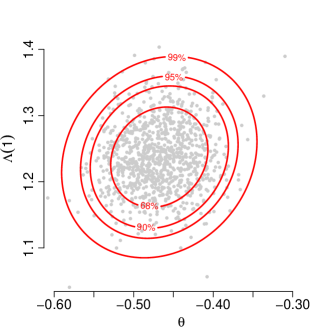
(a)

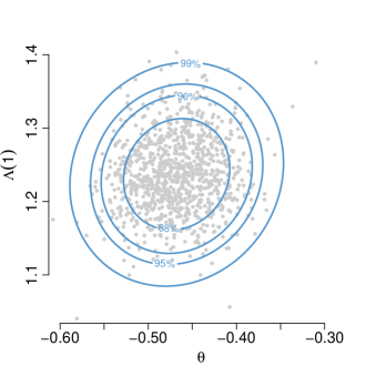
(b)

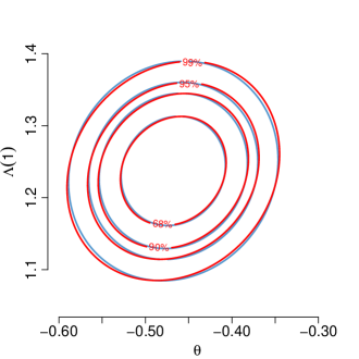
(c)

Figure 4: Contour plots of the elliptical credible sets at the 68%, 90%, 95%, and 99% quantiles. (a) is obtained using the joint limiting distribution given in Corollary 1, (b) is obtained using the 1,000 independent draws of the pair $(\theta,\Lambda(1))$ from the MCMC output. In (c), we overlay the credible sets in (a) and (b). The 1,000 draws are plotted with gray color.

4.3 Study II: Comparing the coverage and the area between the credible bands and the confidence bands

The study in the last section is based on a single simulated dataset. We now provide a more thorough study to compare the coverage and the area of the credible (or confidence) bands under various settings. Specially, we want to compare: 1) the two Bayesian methods using the independent gamma and the dependent gamma priors (while the prior for $\theta$ is chosen to be the standard normal distribution); 2) datasets with two different sample sizes $n=200$ and $n=1,000$; 3) data with two different types of censoring: administrative censoring only and administrative censoring with additional uniform censoring; 4) coverages of the baseline survival function and survival function conditional on $z$ and 5) data are generated from the continuous function in (1) and that from the piecewise constant function in (2).

Two different baseline hazard functions are used to generate the data:

1. $\lambda_{0}(t)=0.8\times\sin(2\pi(t+0.05))+(t+0.05)^{4}-1.8\times(t+0.05)^{2}+2,\ t\in[0,1]$,

1. $\lambda_{0}(t)=3\times\mathbbm{1}_{[0,0.4)}(t)+1.5\times\mathbbm{1}_{[0.4,0.6)}(t)+2\times\mathbbm{1}_{[0.6,1]}(t)$,

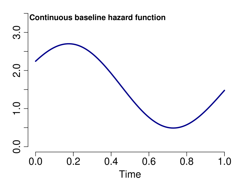
Figure 5: Plot of the continuous baseline hazard function in (1).

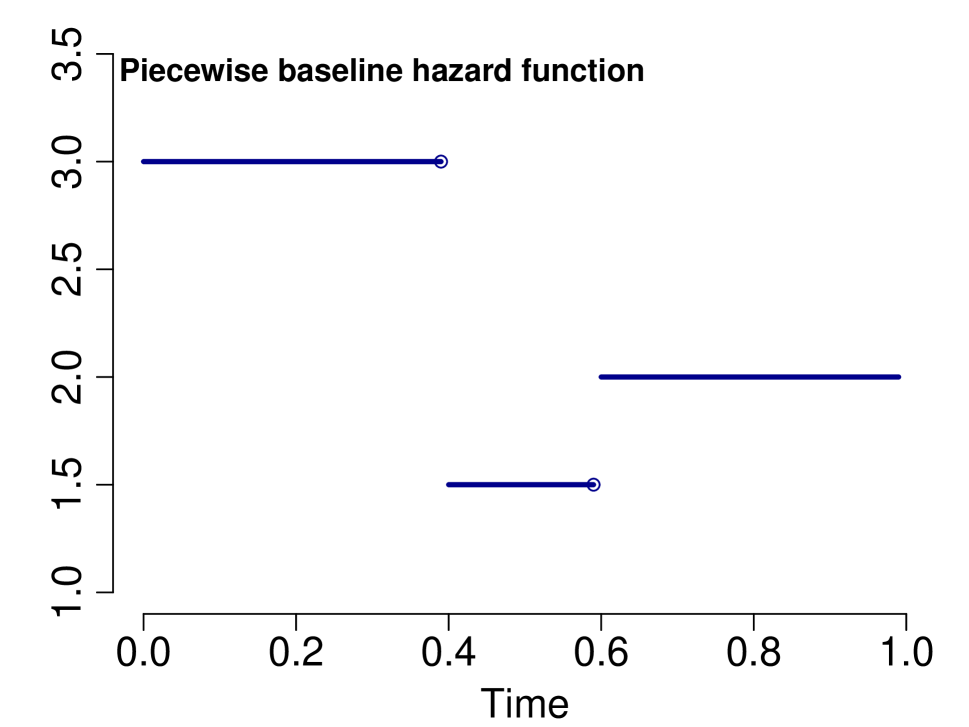
Figure 6: Plot of the piecewise constant baseline hazard function in (2).

The first one is a smooth function and the second one is piecewise constant. Plots of the two functions are given in Figures 6 and 6 respectively. These numerical choices are for illustration purposes and otherwise fairly arbitrary. Similar simulation results would hold if choosing other either smoothly varying or piecewise constant functions (we note once again that, although our theoretical results assume Hölder smoothness of the true log-hazard, the techniques go through for histogram true hazards as well).

For each setting, we generate 1,000 datasets. For each dataset, we run the MCMC sampler to obtain the 95% credible (or confidence) band. The coverage is the percentage of the credible (or confidence) bands encompassing the true function. The area estimated by taking the average of 1,000 areas of the credible (or confidence) bands. Results using the continuous baseline hazard function are given in Table 1 and those using the piecewise constant baseline hazard function are given in Table 2.

Table 1: Coverages and areas of the 95% Bayesian credible bands and of the 95% confidence bands with $\theta_{0}\in\mathbbm{R}^{5}$ and $\lambda_{0}$ is chosen as the continuous function in (1).

	Adm. censoring only				Adm. $+$ Unif. censoring
	baseline survival		cond. survival		baseline survival		cond. survival
	coverage	area	coverage	area	coverage	area	coverage	area
ind. 200	0.96	0.16	0.94	0.16	0.97	0.20	0.96	0.21
dep. 200	0.93	0.16	0.93	0.16	0.92	0.19	0.91	0.19
freq. 200	0.93	0.18	0.93	0.18	0.92	0.22	0.91	0.22
ind. 1000	0.95	0.08	0.93	0.08	0.98	0.10	0.96	0.10
dep. 1000	0.93	0.08	0.92	0.08	0.92	0.09	0.92	0.09
freq. 1000	0.94	0.08	0.93	0.08	0.94	0.10	0.94	0.10

From Table 1, in which $\lambda_{0}$ is chosen to be a continuous function, first, we found that the two Bayesian methods, either using the independent or the dependent gamma prior, produce similar converge results and areas for the credible bands. Second, when $n=200$, the two Bayesian methods yield a smaller area than the frequentist method. The coverages and the areas of the three methods become similar when $n=1,000$. As approximation becomes more accurate when the sample size increases, it is well expected that both the Bayesian approach and the frequentist approach give comparable coverage and area of the confidence band. Third, we found that when data are administratively and uniformly censored, the area of the credible bands is larger than those only administratively censored. Such a result is expected, as we found that in a typical simulated dataset, a former has $\sim$ 40% data are censored, and the latter has $\sim$20% data are censored. Last, there is no significant difference between the coverage and the area of the baseline survival function and the survival function conditional on $z$, even though the latter accounts for the uncertainty for estimating the regression coefficients.

Table 2: Coverages and areas of the 95% Bayesian credible bands and of the 95% confidence bands with $\theta_{0}\in\mathbbm{R}^{5}$ and $\lambda_{0}$ is chosen as the piecewise constant function in (2).

	Adm. censoring only				Adm. $+$ Unif. censoring
	baseline survival		cond. survival		baseline survival		cond. survival
	coverage	area	coverage	area	coverage	area	coverage	area
ind. 200	0.94	0.15	0.93	0.15	0.96	0.08	0.95	0.18
dep. 200	0.95	0.15	0.94	0.15	0.93	0.18	0.93	0.18
freq. 200	0.94	0.17	0.94	0.17	0.90	0.21	0.90	0.21
ind. 1000	0.95	0.09	0.93	0.07	0.95	0.09	0.94	0.09
dep. 1000	0.93	0.07	0.93	0.07	0.93	0.09	0.92	0.09
freq. 1000	0.93	0.07	0.93	0.08	0.92	0.10	0.92	0.10

Table 2 gives the results for data are generated from the baseline hazard that is the piecewise constant function in (2). We observe similar results for the coverage of the frequentist confidence bands as in Table 1. We also observe that the area of the credible bands provided by the two Bayesian methods is smaller than that of the confidence bands. We also found that both of the two Bayesian methods provide similar coverage results whether $\lambda_{0}$ is chosen to be the continuous function or the piecewise constant function.

In summary, using the Bayesian method can be attractive for estimating data with a relatively small sample size, as it gives a smaller area. The frequentist method needs to apply an asymptotical approximation to obtain the confidence band, and the approximation can perform slightly poorly when the sample size is relatively small. On the other hand, the proposed Bayesian method provides a credible band without using any asymptotical approximation. Notice that the width for the credible band is constant over time. It should be possible to build a varying-width credible band whose overall area is smaller, both in small samples and asymptotically, but the construction and analysis of such a band is outside the scope of the paper. Yet, the considered fixed–width credible band performs already remarkably well, in particular in finite samples, and achieves the asymptotic limits expected from the Donsker theorem for large sample sizes.

5 Discussion

We provide three new exciting results for the study of the Bayesian Cox model: 1) a joint Bernstein–von Mises theorem for the linear functionals of $\theta$ and $\lambda$; in particular, the correlation between the two functionals is captured by the results; 2) a Bayesian Donsker theorem for the hazard function conditional on $z$ and the survival function conditional on $z$; 3) a supremum-norm posterior contraction rate for the hazard function conditional on $z$.

The paper makes major advances on two fronts: on the one hand, it provides new results on optimal posterior convergence rates both in $L^{1}$– and $L^{\infty}$–sense for the hazard; uncertainty quantification is considered for finite dimensional functionals as well as for the posterior cumulative hazard process: those are the first results of this kind for non–conjugate priors (in particular priors for which explicit posterior expressions are not accessible) in this model. On the other hand, the paper provides validation for several classes of practically used histogram priors (see e.g. Ibrahim et al. (2001)), both for dependent and independent histogram heights.

As a comparison, the results from Castillo (2012) (Theorem 5) and Ghosal and van der Vaart (2017) (Theorem 12.12) require a fast enough preliminary posterior contraction rate of $n^{-3/8}$ in terms of the Hellinger distance. This effectively rules out the use of regular histogram priors, which are limited in terms of rate by $n^{-1/3}$ (corresponding to the optimal minimax rate for Lipschitz functions). Two key novelties here are that a) we only require a preliminary rate of an order faster than $n^{-1/4}$ (corresponding to $\beta=1/2$ in (11)) b) the use of the multiscale approach introduced in Castillo and Nickl (2014) enables one to provide both optimal supremum norm contraction rates for the conditional hazard, justifying practically the visual closeness of estimated hazard curves to the true curve, and uncertainty quantification for the conditional cumulative hazard, which follows a BvM for $\Lambda(\cdot)e^{\theta^{\prime}z}$.

Comparing to Castillo and van der Pas (2021a) which studied the nonparametric right-censoring model, we would like to highlight the challenges that are unique to our study of the Cox model: First, deriving the joint Bernstein-von Mises (BvM) results for the Cox model is more challenging than for the right-censoring model as one needs to construct local paths for both $\theta$ and $\lambda$ in (14)-(15). Our construction of these local paths in multi-dimensions, and jointly with linear functionals of the hazard, is new.

Second, one needs to invoke Proposition S2 in Ning and Castillo (2023) to obtain the joint nonparametric BvM theorem. This is in contrast with the study of the right-censoring model, for which Proposition 6 of Castillo and Nickl (2014) can be used directly for handling a single non-parametric quantity. Hence, the study of semiparametric models, including the Cox model, requires an extended argument. It is worth mentioning that these results can be useful for studying other semiparametric models in the future. In particular the joint and multidimensional BvMs obtained here are new and could be obtained elsewhere by following our arguments.

Third, controlling the LAN reminder terms and the semiparametric bias are significantly more complex tasks for the Cox model. This essentially leads to the requirement of the regularity $\beta>1/2$. This requirement seems to be unavoidable with the current proof techniques.

Last, in practice, confidence bands for the survival function of the Cox model are not commonplace; however, for the right-censoring method, confidence bands for survival functions are routinely used. We are not aware of an easy-to-implement computational algorithm for obtaining the confidence band. An additional contribution of our paper is that we showed that this band could be easily obtained by using the Bayesian approach introduced here.

We also underline that although not investigated here in details for reasons of space, the results extend to smoother dictionaries than histograms: for instance, if the true hazard is very smooth, one can derive correspondingly very fast posterior rates (obtaining optimal rates $n^{-\beta/(2\beta+1)}$ for any $\beta>1/2$, up to log factors) if one chooses the basis $(\psi_{lk})$ to be a suitably smooth wavelet basis. We refer the interested reader to Castillo and van der Pas (2021a) for more on how to effectively obtain this. For the frequentist approach considered in this article, the Breslow estimator, which treats the $\lambda_{0}$ as piecewise constant between uncensored failure times (see Page 473 of Lin, 2007), can also be replaced by a smoother estimate, e.g. by taking the kernel-smoothing approach as in Ramlau-Hansen (1983) and Guilloux et al. (2016) to model smooth baseline hazard functions.

The present work studies the classical Cox model. Many extensions of the model have been proposed, such as the Cox model with time-varying covariates (Fisher and Lin, 1999), the nonproportional hazards model (Schemper, 2002), the Cox-Aalan model (Scheike and Zhang, 2002) to name a few. The Bayesian nonparametric perspective is particularly appealing in these more complex settings; let us cite two recent practical success stories of the approach in settings going beyond the Cox model (in particular enabling more complex dependencies in terms of covariates and hazard, and/or time dependence): one is the use of BART (Bayesian additive regression trees) priors in Sparapani et al. (2016), another is the use of dependent Dirichlet process priors in Xu et al. (2019). It would be very desirable to obtain theory and validation for these more complex settings: the present work can be seen as a first step towards this aim.

6 Proof of Theorem 3.2

In this section, we prove Theorem 3.2. Section 6.1 provides the necessary background for studying the Cox model, including the expressions of the LAN-norm, the LAN expansion, the log-likelihood ratio, the squared Hellinger distance between $f_{\eta}$ and $f_{\eta_{0}}$, and the relation between the random histogram and Haar wavelets. The relation is useful for studying the histogram priors in Section 2.4 as one could invoke results based on the use of Haar wavelets priors directly. The main proof of Theorem 3.2 is given in Section 6.2. The proofs of the remaining theorems and lemmas in Section 3 are given in the Supplemental Materials (Ning and Castillo, 2023).

6.1 Background

We first review several properties of the Cox model that will be frequently used in the proofs of the theorems:

1. Let us introduce the Hilbert inner product between $(\vartheta_{1},g_{1})$ and $(\vartheta_{2},g_{2})$, for any $\vartheta_{1},\vartheta_{2}\in\mathbb{R}^{p}$ and any $g_{1},g_{2}\in L^{2}(\Lambda_{0})$, as

   $$\langle(\vartheta_{1},g_{1}),(\vartheta_{2},g_{2})\rangle_{L}=\Lambda_{0}\left\{\vartheta_{1}^{\prime}M_{2}(\cdot)\vartheta_{2}+(g_{1}(\cdot)\vartheta_{2}^{\prime}+g_{2}(\cdot)\vartheta_{1}^{\prime})M_{1}(\cdot)+g_{1}(\cdot)g_{2}(\cdot)M_{0}(\cdot)\right\}.$$ (26)

   This inner-product features in the likelihood expansion (also called Locally Asymptotically Normal expansion or LAN) in the next point and is simply called LAN norm.

2. For the log-likelihood ratio given in (2), the LAN expansion for this log-likelihood ratio can be written as

   $$\ell_{n}(\eta)-\ell_{n}(\eta_{0})=-\frac{n}{2}\|\theta-\theta_{0},r-r_{0}\|^{2}_{L}+\sqrt{n}W_{n}(\theta-\theta_{0},r-r_{0})+R_{n}(\eta,\eta_{0}),$$ (27)

   where

   $$\begin{split}\|\theta-\theta_{0},r-r_{0}\|_{L}^{2}=\Lambda_{0}\big{\{}&(\theta-\theta_{0})^{\prime}M_{2}(u)(\theta-\theta_{0})+2(r-r_{0})(u)(\theta-\theta_{0})^{\prime}M_{1}(u)\\ &+(r-r_{0})^{2}(u)M_{0}(u)\big{\}},\end{split}$$ (28)

   is the LAN-norm part,

   $$\begin{split}W_{n}(\theta-\theta_{0},r-r_{0})=\frac{1}{\sqrt{n}}\sum_{i=1}^{n}\big{\{}&\delta_{i}\big{(}(\theta-\theta_{0})^{\prime}Z_{i}+(r-r_{0})(Y_{i})\big{)}-e^{\theta_{0}^{\prime}Z_{i}}\big{(}(\theta-\theta_{0})^{\prime}Z_{i}\Lambda_{0}(Y_{i})\\ &+(\Lambda_{0}(r-r_{0}))(Y_{i})\big{)}\big{\}},\end{split}$$ (29)

   is the stochastic part, and $R_{n}(\eta,\eta_{0})$ is the remainder part, which can be further written as

   $$R_{n}(\eta,\eta_{0})=R_{n,1}(\eta,\eta_{0})+R_{n,2}(\eta,\eta_{0}),$$ (30)

   where

   $$R_{n,1}(\eta,\eta_{0})=-\mathbb{G}_{n}\Psi_{n}(\eta).$$ (31)

   For a measurable function $f$, $\mathbb{G}_{n}(f)=\frac{1}{\sqrt{n}}\sum_{i=1}^{n}(f(X_{i})-P_{\eta_{0}}f),$ which is the centered and scaled version of the empirical measure, and

   $$\begin{split}\Psi_{n}(\eta)(X_{i})=\sqrt{n}\Big{\{}&e^{\theta^{\prime}Z_{i}}\Lambda_{0}\{e^{r-r_{0}}\}(Y_{i})-e^{\theta_{0}^{\prime}Z_{i}}\Lambda_{0}(Y_{i})-e^{\theta_{0}^{\prime}Z_{i}}(\theta-\theta_{0})^{\prime}Z_{i}\Lambda_{0}(Y_{i})\\ &-e^{\theta_{0}^{\prime}Z_{i}}\Lambda_{0}\{r-r_{0}\}(Y_{i})\Big{\}}.\end{split}$$

   Let

   $$M_{0}(\theta)(\cdot)=\mathbb{E}_{\eta_{0}}(\mathbbm{1}_{u\leq Y}e^{\theta^{\prime}Z})=\int\bar{G}_{z}(u)e^{\theta^{\prime}z}e^{-\Lambda_{0}(u)e^{\theta_{0}^{\prime}z}}f_{Z}(z)dz,$$ (32)

   and $M_{0}(\cdot)$ and $M_{1}(\cdot)$ in (3) and (4) respectively,

   $$\begin{split}R_{n,2}(\eta,\eta_{0})=&-n\Lambda_{0}\Big{\{}M_{0}(\theta)(\cdot)e^{(r-r_{0})(\cdot)}-M_{0}(\cdot)-(\theta-\theta_{0})^{\prime}M_{1}(\cdot)\\ &-(r-r_{0})(\cdot)M_{0}(\cdot)\Big{\}}+\frac{n}{2}\|\theta-\theta_{0},r-r_{0}\|_{L}^{2}.\end{split}$$ (33)

3. Recall that $\gamma_{M_{1}}=M_{1}/M_{0}$ is the least favorable direction and $\tilde{I}_{\eta_{0}}$ is the efficient information matrix in (6), the LAN-norm in (28) can be also written as

   $$\|\theta-\theta_{0},r-r_{0}\|_{L}^{2}=(\theta-\theta_{0})^{\prime}\tilde{I}_{\eta_{0}}(\theta-\theta_{0})+\|0,r-r_{0}+\gamma_{M_{1}}^{\prime}(\theta-\theta_{0})\|_{L}^{2}.$$ (34)

4. For the density function in (1), the squared Hellinger distance between $f_{\eta}$ and $f_{\eta_{0}}$ is

   $$h^{2}(f_{\eta},f_{\eta_{0}}) =\int\int_{0}^{1}\left[\sqrt{S_{\eta}}-\sqrt{S_{\eta_{0}}}\right]^{2}(u,z)g_{z}(u)f_{Z}(z)dudz$$ (35)

   $$\quad+\int\int_{0}^{1}\bar{G}_{z}(u)\left[\sqrt{\lambda S_{\eta}e^{\theta^{\prime}z}}-\sqrt{\lambda_{0}S_{\eta_{0}}e^{\theta_{0}^{\prime}z}}\right]^{2}(u,z)f_{Z}(z)dudz$$ (36)

   $$\quad+\int\bar{G}_{z}(1)\left[\sqrt{S_{\eta}}-\sqrt{S_{\eta_{0}}}\right]^{2}(1,z)f_{Z}(z)dz,$$ (37)

   where we slightly abuse the notation by denoting $S_{\eta}(u,z)=e^{-\Lambda_{0}(u)e^{\theta^{\prime}z}}$. A similar expression appears on page 34 of Castillo (2012) (up to a typo in the third term in his expression, fixed in the last display)

We also review the relation between the random histogram and Haar wavelets. Let’s denote $r_{H}=(r_{1},\dots,r_{2^{L}+1})^{\prime}$, where $r_{H}=\log\lambda_{H}$, as the step heights of the random histogram and $r_{S}=(r_{-1},r_{00},r_{01},\dots,r_{L(2^{L}-1)})^{\prime}$ as the coefficients in the Haar wavelet prior, then through Haar transformation,

$$r_{S}=\Psi r_{H}$$ (38)

where for $I_{k}^{l}=(k2^{-l},(k+1)2^{-l}]$,

$$\Psi_{-1,j}=2^{-(L+1)},\quad\Psi_{lk,j}=2^{-(L+1)+l/2}[\mathbbm{1}_{I_{j-1}^{L+1}\subset I_{2k}^{l+1}}-\mathbbm{1}_{I_{j-1}^{L+1}\subset I_{2k+1}^{l+1}}],$$

and $2^{(L+1)/2}\Psi$ is an orthogonal matrix.

Last, as the posterior concentrates on the set $\|\lambda-\lambda_{0}\|_{\infty}\leq\zeta_{n}$ in Lemma 1, we use the fact that

$$\lambda-\lambda_{0}=e^{r}-e^{r_{0}}=e^{r_{0}}\left(e^{r-r_{0}}-1\right);$$

therefore, as long as $\zeta_{n}=o(1)$ which is the case since $\beta>1/2$, by Taylor’s theorem and assumption (iii) such that $\|\lambda_{0}\|_{\infty}$ by some constant, $\|\lambda-\lambda_{0}\|_{\infty}=O(\zeta_{n})$ automatically translates into the same rate for $\|r-r_{0}\|_{\infty}$. This fact will be automatically applied in our proofs.

6.2 Proof of the main theorem

We now prove Theorem 3.2. We follow Castillo and Rousseau (2015a) and show that the Laplace transform of the induced posterior distribution on the functional of interest converges to the corresponding Laplace transform of the optimal (efficient) Gaussian limit. From Lemma 1 and Lemma 2 of Castillo and Rousseau (2015b), it is sufficient to show that the Laplace transform of the induced posterior distribution on the functional of interest in (16) converges to the corresponding Laplace transform of the optimal (efficient) Gaussian limit. That is, define $\varphi_{a}(\theta)=\theta^{\prime}a$, $\varphi_{b}(\lambda)=\int\lambda b$ and let $\hat{\varphi}_{a}=\varphi_{a}(\theta_{0})+W_{n}^{(1)}(a)/\sqrt{n}$ and $\hat{\varphi}_{b}=\varphi_{b}(\lambda_{0})+W_{n}^{(2)}(b)/\sqrt{n}$, where

$$W_{n}^{(1)}(a)=W_{n}(\tilde{I}_{\eta_{0}}^{-1}a,\ -\gamma_{M_{1}}^{\prime}\tilde{I}_{\eta_{0}}^{-1}a),$$

$$W_{n}^{(2)}(b)=W_{n}\left(-\tilde{I}_{\eta_{0}}^{-1}\Lambda_{0}\{b\gamma_{M_{1}}\},\ \gamma_{b}+\gamma_{M_{1}}^{\prime}\tilde{I}_{\eta_{0}}^{-1}\Lambda_{0}\{b\gamma_{M_{1}}\}\right),$$

and $W_{n}(\cdot,\cdot)$ is given in (29), our goal is to show that for any $h=(t,s)\in\mathbb{R}^{2}$,

$$\mathbb{E}\left[e^{\sqrt{n}h\left(\varphi_{a}(\theta)-\hat{\varphi}_{a},\ \varphi_{b}(\lambda)-\hat{\varphi}_{b}\right)^{\prime}}\,|\,X,A_{n}\right]\stackrel{{\scriptstyle P_{\eta_{0}}}}{{\to}}e^{h\Sigma_{a,b}h^{\prime}/2},$$ (39)

where

$$\Sigma_{a,b}=\begin{pmatrix}a^{\prime}\tilde{I}_{\eta_{0}}^{-1}a&-a^{\prime}\tilde{I}_{\eta_{0}}^{-1}\Lambda_{0}\{b\gamma_{M_{1}}\}\\ -a^{\prime}\tilde{I}_{\eta_{0}}^{-1}\Lambda_{0}\{b\gamma_{M_{1}}\}&\Lambda_{0}\{b\gamma_{b}\}+\Lambda_{0}\{b\gamma_{M_{1}}^{\prime}\}\tilde{I}_{\eta_{0}}^{-1}\Lambda_{0}\{b\gamma_{M_{1}}\}\end{pmatrix}.$$ (40)

By applying Bayes’ formula and dividing the expression at the right hand side on both side of (39), the display in (39) can be written as

$$\frac{\int_{A_{n}}e^{\sqrt{n}h(\varphi_{a}(\theta)-\hat{\varphi}_{a},\varphi_{b}(\lambda)-\hat{\varphi}_{b})^{\prime}+\ell_{n}(\eta)-\ell_{n}(\eta_{0})-h^{\prime}\Sigma_{a,b}h/2}d\Pi(\eta)}{\Pi(A_{n}\,|\,X)\int e^{\ell_{n}(\eta)-\ell_{n}(\eta_{0})}d\Pi(\eta)}\stackrel{{\scriptstyle P_{\eta_{0}}}}{{\to}}1.$$ (41)

Below, we will provide the key steps for proving (41). Intermediate lemmata along with their proofs are left to Section S3 in the supplemental material.

To bound the numerator at the left hand side of (41), an important step is to show that

$$\begin{split}&\sup_{\eta\in A_{n}}|\sqrt{n}h(\varphi_{a}(\theta)-\hat{\varphi}_{a},\varphi_{b}(\lambda)-\hat{\varphi}_{b})^{\prime}+\ell_{n}(\eta)-\ell_{n}(\eta_{0})-h^{\prime}\Sigma_{a,b}h/2|\\ &\quad\leq\sup_{\eta\in A_{n}}|\ell_{n}(\eta_{h})-\ell_{n}(\eta_{0})|+o(1)+o_{P_{\eta_{0}}}(1),\end{split}$$ (42)

where $\eta_{h}=(\theta_{h},r_{h})$, and $\theta_{h}$ and $r_{h}$ are given in (14) and (15) respectively.

To prove (42), using the expression of the LAN-norm given in (27) and note that one can write $\ell_{n}(\eta)-\ell_{n}(\eta_{0})=\ell_{n}(\eta)-\ell_{n}(\eta_{0})-[\ell_{n}(\eta_{h})-\ell_{n}(\eta_{0})]+\ell_{n}(\eta_{h})-\ell_{n}(\eta_{0})$ and then obtain

$$\ell_{n}(\eta)-\ell_{n}(\eta_{0})-[\ell_{n}(\eta_{h})-\ell_{n}(\eta_{0})]$$

$$\quad=-\frac{n}{2}\left(\|\theta-\theta_{0},r-r_{0}\|_{L}^{2}-\|\theta_{h}-\theta_{0},r_{h}-r_{0}\|_{L}^{2}\right)$$ (43)

$$\qquad+\sqrt{n}\left(W_{n}(\theta-\theta_{0},r-r_{0})-W_{n}(\theta_{h}-\theta_{0},r_{h}-r_{0})\right)$$ (44)

$$\qquad+R_{n}(\eta,\eta_{0})-R_{n}(\eta_{h},\eta_{0}),$$ (45)

where $\|\cdot,\cdot\|_{L}$, $W_{n}(\cdot,\cdot)$, and $R_{n}(\cdot,\cdot)$ are defined in (28), (29), and (30) respectively.

On the other hand, we write $(\theta-\theta_{0})^{\prime}a$ and $\Lambda\{b\}-\Lambda_{0}\{b\}$ as their LAN-norm Hilbert inner product forms, i.e.,

$$(\theta -\theta_{0})^{\prime}a=\left\langle(\theta-\theta_{0},r-r_{0}),\left(\tilde{I}_{\eta_{0}}^{-1}a,-\gamma_{M_{1}}^{\prime}\tilde{I}_{\eta_{0}}^{-1}a\right)\right\rangle_{L},$$ (46)

$$\Lambda\{b\}-\Lambda_{0}\{b\} =\left\langle\left(\theta-\theta_{0},\frac{\lambda-\lambda_{0}}{\lambda_{0}}\right),\left(-\tilde{I}_{\eta_{0}}^{-1}\Lambda_{0}\{b\gamma_{M_{1}}\},\gamma_{b}+\gamma_{M_{1}}^{\prime}\tilde{I}_{\eta_{0}}^{-1}\Lambda_{0}\{b\gamma_{M_{1}}\}\right)\right\rangle_{L}.$$ (47)

by using fact that (also, see (26)) the LAN-norm Hilbert inner product between $(\vartheta_{1},g_{1})$ and $(\vartheta_{2},g_{2})$, for any $\vartheta_{1},\vartheta_{2}\in\mathbb{R}^{p}$ and any $g_{1},g_{2}\in L^{2}(\Lambda_{0})$, is defined as

$$\langle(\vartheta_{1},g_{1}),(\vartheta_{2},g_{2})\rangle_{L}=\Lambda_{0}\left\{\vartheta_{1}^{\prime}M_{2}(\cdot)\vartheta_{2}+(g_{1}(\cdot)\vartheta_{2}^{\prime}+g_{2}(\cdot)\vartheta_{1}^{\prime})M_{1}(\cdot)+g_{1}(\cdot)g_{2}(\cdot)M_{0}(\cdot)\right\}.$$

The right hand side of (47) can be further decomposed into three parts such that

$$\Lambda\{b\}-\Lambda_{0}\{b\}=B_{1}(\eta,\eta_{0})+B_{2}(\eta,\eta_{0})-B_{3}(\eta,\eta_{0}),$$ (48)

where

$$B_{1}(\eta,\eta_{0})=\left\langle\left(\theta-\theta_{0},r-r_{0}\right),\left(-\tilde{I}_{\eta_{0}}^{-1}\Lambda_{0}\{b\gamma_{M_{1}}\},\gamma_{b,L_{n}}+\gamma_{M_{1},L_{n}}^{\prime}\tilde{I}_{\eta_{0}}^{-1}\Lambda_{0}\{b\gamma_{M_{1}}\}\right)\right\rangle_{L},$$ (49)

$$B_{2}(\eta,\eta_{0})=\left\langle\left(0,\frac{\lambda-\lambda_{0}}{\lambda_{0}}\right),\left(0,\gamma_{b}-\gamma_{b,L_{n}}+(\gamma_{M_{1}}-\gamma_{M_{1},L_{n}})^{\prime}\tilde{I}_{\eta_{0}}^{-1}\Lambda_{0}\{b\gamma_{M_{1}}\}\right)\right\rangle_{L},$$ (50)

$$B_{3}(\eta,\eta_{0})=\left\langle\left(0,r-r_{0}-\frac{\lambda-\lambda_{0}}{\lambda_{0}}\right),\left(-\tilde{I}_{\eta_{0}}^{-1}\Lambda_{0}\{b\gamma_{M_{1}}\},\gamma_{b,L_{n}}+\gamma_{M_{1},L_{n}}^{\prime}\tilde{I}_{\eta_{0}}^{-1}\Lambda_{0}\{b\gamma_{M_{1}}\}\right)\right\rangle_{L}.$$ (51)

The third term (51) is a semiparametric bias.

Now we plug (43)-(45) and (48) into (42) and note that $\hat{\varphi}_{a}=\theta_{0}^{\prime}a+W_{n}^{(1)}(a)/\sqrt{n}$ and $\hat{\varphi}_{b}=\Lambda_{0}\{b\}+W_{n}^{(2)}(b)/\sqrt{n}$, then the left hand side of (42) can be written as

$$\sqrt{n}h(\varphi_{a}(\theta)-\hat{\varphi}_{a},\varphi_{b}(\lambda)-\hat{\varphi}_{b})^{\prime}+\ell_{n}(\eta)-\ell_{n}(\eta_{0})-[\ell_{n}(\eta_{h})-\ell_{n}(\eta_{0})]-h^{\prime}\Sigma_{a,b}h/2$$

$$\quad=t\sqrt{n}(\theta-\theta_{0})^{\prime}a+s\sqrt{n}B_{1}(\eta,\eta_{0})-\frac{n}{2}(\|\theta-\theta_{0},r-r_{0}\|_{L}^{2}-\|\theta_{h}-\theta_{0},r_{h}-r_{0}\|_{L}^{2})$$ (52)

$$\qquad+s\sqrt{n}B_{2}(\eta,\eta_{0})-{h^{\prime}\Sigma_{a,b}h}/{2}+R_{n}(\eta,\eta_{0})-R_{n}(\eta_{h},\eta_{0})-s\sqrt{n}B_{3}(\eta,\eta_{0})$$ (53)

$$\qquad-tW_{n}^{(1)}(a)-sW_{n}^{(2)}(b)+\sqrt{n}W_{n}(\theta-\theta_{0},r-r_{0})-\sqrt{n}W_{n}(\theta_{h}-\theta_{0},r_{h}-r_{0}).$$ (54)

Thus to proof (42), one needs to show the last display is bounded by $o(1)+o_{P_{\eta_{0}}}(1)$ uniformly on the set $\eta\in A_{n}$. We will bound each line in the last display:

1. To bound (52), by plugging-in the expressions of $\theta_{h}$, $r_{h}$, and (46), one can check that

   $$t\sqrt{n}(\theta-\theta_{0})^{\prime}a+s\sqrt{n}B_{1}(\eta,\eta_{0})=n\langle(\theta-\theta_{0},r-r_{0}),(\theta-\theta_{h},r-r_{h})\rangle_{L}.$$

   Also, note that $\langle(\theta_{h}-\theta_{0},r_{h}-r_{0})\rangle_{L}=\langle(\theta_{h}-\theta,r_{h}-r)\rangle_{L}+\langle(\theta-\theta_{0},r-r_{0})\rangle_{L},$ by expanding the two squared LAN-norms in (52), we have

   $$n\langle(\theta-\theta_{0},r-r_{0}),(\theta-\theta_{h},r-r_{h})\rangle_{L}-\frac{n}{2}\|\theta-\theta_{0},r-r_{0}\|_{L}^{2}+\frac{n}{2}\|\theta_{h}-\theta_{0},r_{h}-r_{0}\|_{L}^{2}$$

   $$\quad=\frac{n}{2}\|\theta-\theta_{h},r-r_{h}\|_{L}^{2}.$$

   Define

   $$D_{n} =\frac{n}{2}\|\theta-\theta_{h},r-r_{h}\|_{L}^{2}-\frac{h^{\prime}\Sigma_{a,b}h}{2}.$$ (55)

   Note that the expression in (52) equals to $D_{n}$. By invoking Lemma S9 in the supplemental material, we obtain

   $$\sup_{\eta\in A_{n}}|D_{n}| \leq s^{2}\|\gamma_{b}^{2}-\gamma_{b,L_{n}}^{2}\|_{1}+(t^{2}+s^{2})(p^{2}2^{-L_{n}}\|\gamma_{b,L_{n}}\|_{1}+p^{4}2^{-2L_{n}}).$$

   To bound the last display, we first invoke Lemma S19 in the supplemental material to obtain $\|\gamma_{b,L_{n}}\|_{1}\leq\|\gamma_{b,L_{n}}\|_{2}\lesssim\|b\|_{2}$. Then applying the inequality $\|fg\|_{1}\leq\|f\|_{1}\|g\|_{\infty}$ and using (B) to obtain the bound $\|\gamma_{b}^{2}-\gamma_{b,L_{n}}^{2}\|_{1}\leq(\|\gamma_{b}\|_{1}+\|\gamma_{b,L_{n}}\|_{1})(\|\gamma_{b}-\gamma_{b,L_{n}}\|_{\infty})\leq(\|\gamma_{b}\|_{1}+\|\gamma_{b,L_{n}}\|_{1})/(\sqrt{n}\epsilon_{n})$. Since $b\in L^{\infty}([0,1])$ and $p,t,s$ are constants, by plugging-in the two upper bounds, the last display is bounded by $s^{2}\|b\|_{2}/(\sqrt{n}\epsilon_{n})+p^{2}2^{-L_{n}}\|b\|_{2}+o(1),$ which is $o(1)$, as $\sqrt{n}\epsilon_{n}\to\infty$ and $L_{n}\to\infty$ as $n\to\infty$.

2. To bound (53), we first deal with the first term. By (S20) in Lemma S8,

   $$\sqrt{n}\sup_{\eta\in A_{n}}|sB_{2}(\eta,\eta_{0})|\lesssim|s|\sqrt{n}\epsilon_{n}\|\gamma_{b}-\gamma_{b,L_{n}}\|_{\infty}+|s|p^{2}\sqrt{n}\epsilon_{n}2^{-L_{n}}\|b\|_{1}.$$

   Using (B) and the assumption $\sqrt{n}\epsilon_{n}2^{-L_{n}}=o(1)$, note that $b\in L^{\infty}([0,1])$, the last display is $o(1)$.

   To bound the last three terms in (53), from (30), $R_{n}(\eta,\eta_{0})=R_{n,1}(\eta,\eta_{0})+R_{n,2}(\eta,\eta_{0})$, where the expressions of $R_{n,1}(\eta,\eta_{0})$ and $R_{n,2}(\eta,\eta_{0})$ are given in (31) and (33) respectively. Then,

   $$\begin{split}&\sup_{\eta\in A_{n}}|R_{n}(\eta,\eta_{0})-R_{n}(\eta_{h},\eta_{0})-s\sqrt{n}B_{3}(\eta,\eta_{0})|\\ &\quad\leq\sup_{\eta\in A_{n}}|R_{n,1}(\eta,\eta_{0})-R_{n,1}(\eta_{h},\eta_{0})|\\ &\quad\quad+\sup_{\eta\in A_{n}}|R_{n,2}(\eta,\eta_{0})-R_{n,2}(\eta_{h},\eta_{0})-s\sqrt{n}B_{3}(\eta,\eta_{0})|.\end{split}$$ (56)

   We apply Lemma S11 in the supplemental material to bound the first term in the last display. To verify the conditions in Lemma S11, since $\|a\|_{\infty}$ is bounded and $b\in L^{\infty}([0,1])$, for $\Delta_{1}$ and $\Delta_{2,L_{n}}$ defined in (S28) and (S29) in the supplemental material, it is easy to check that both $\Delta_{1}/\sqrt{n}=o(1)$ and $\Delta_{2,L_{n}}/\sqrt{n}=o(1)$ by applying triangular inequalities. Thus we can invoke Lemma S11 to obtain

   $$\sup_{\eta\in A_{n}}|R_{n,1}(\eta,\eta_{0})-R_{n,1}(\eta_{h},\eta_{0})|\leq O_{P_{\eta_{0}}}\left(L_{n}^{2}/\sqrt{n}+\epsilon_{n}L_{n}\right)=o_{P_{\eta_{0}}}(1),$$

   as $L_{n}^{2}/\sqrt{n}=o(1)$ and $\epsilon_{n}L_{n}=o(1)$ by assumptions.

   To bound the last line in (56), define $K_{a,b,t,s}=p^{2}(|t|\|a\|_{\infty}+|s|\|b\|_{1})+|s|\|b\|_{\infty}$ and $\tilde{K}_{a,b,t,s}=p^{2}(|t|\|a\|_{\infty}+|s|\|b\|_{1})+|s|\|b\|_{2}$. Since $t,s,p$ are all fixed constants, $\|a\|_{\infty}$ is bounded, and $b\in L^{\infty}([0,1])$, then $K_{a,b,t,s}=O(1)$ and $\tilde{K}_{a,b,t,s}=O(1)$. By invoking Lemma S12 in the supplemental material, we have

   $$\sup_{\eta\in A_{n}}|R_{n,2}(\eta,\eta_{0})-R_{n,2}(\eta_{h},\eta_{0})-s\sqrt{n}B_{3}(\eta,\eta_{0})|$$

   $$\quad\lesssim\tilde{K}_{a,b,t,s}^{3}/\sqrt{n}+K^{2}_{a,b,h,p}L_{n}^{2}\epsilon_{n}+|s|p^{2}\sqrt{n}\epsilon_{n}2^{-L_{n}}+\sqrt{n}\epsilon_{n}^{2}L_{n}K_{a,b,t,s}$$

   $$\quad\lesssim L_{n}^{2}\epsilon_{n}+\sqrt{n}\epsilon_{n}2^{-L_{n}}+\sqrt{n}\epsilon_{n}^{2}L_{n},$$

   which is $o(1)$ as $\epsilon_{n}L_{n}=o(1)$ and $\sqrt{n}\epsilon_{n}^{2}L_{n}=o(1)$ by assumption. We thus showed that (53) is $o_{P_{\eta_{0}}}(1)$ for $\eta\in A_{n}$.

3. To bound (54), we directly plug-in the expressions of $\theta_{h}$ and $r_{h}$ to obtain

   $$\sqrt{n}W_{n}(\theta-\theta_{0},r-r_{0})-\sqrt{n}W_{n}(\theta_{h}-\theta_{0},r_{h}-r_{0})$$

   $$\quad=W_{n}(t\tilde{I}_{\eta_{0}}^{-1}a-s\tilde{I}_{\eta_{0}}^{-1}\Lambda_{0}\{b\gamma_{M_{1}}\},\ -t\gamma_{M_{1},L_{n}}^{\prime}\tilde{I}_{\eta_{0}}^{-1}a+s\gamma_{b,L_{n}}+s\gamma_{M_{1},L_{n}}^{\prime}\tilde{I}_{\eta_{0}}^{-1}\Lambda_{0}\{b\gamma_{M_{1}}\}).$$

   Due to the linearity of $W_{n}(\cdot,\cdot)$, (54) can be also written as

   $${W_{n}(0,t(\gamma_{M_{1}}-\gamma_{M_{1},L_{n}})^{\prime}\tilde{I}_{\eta_{0}}^{-1}a)}-{W_{n}(0,s(\gamma_{b}-\gamma_{b,L_{n}}))}-{W_{n}(0,s(\gamma_{M_{1}}-\gamma_{M_{1},L_{n}})^{\prime}\tilde{I}_{\eta_{0}}^{-1}\Lambda_{0}(b\gamma_{M_{1}}))}.$$

   Applying the fourth point of Lemma S21 in the supplemental material and using the fact that $2^{-L_{n}/2}=o(1)$ as $n\to\infty$, the second term in the last display is $o_{P_{\eta_{0}}}(1)$. To bound the first term in the last display, since $p,t,s$ are fixed constants and $\|a\|_{\infty}$ is bounded, by (v), we have

   $$|t(\gamma_{M_{1}}-\gamma_{M_{1},L_{n}})^{\prime}\tilde{I}_{\eta_{0}}^{-1}a| \leq|t|p^{2}\|a\|_{\infty}\|\tilde{I}_{\eta_{0}}^{-1}\|_{(\infty,\infty)}\max_{j}\|\gamma_{M_{1}}^{j}-\gamma_{M_{1},L_{n}}^{j}\|_{\infty}$$

   $$\lesssim\max_{j}\|\gamma_{M_{1}}^{j}-\gamma_{M_{1},L_{n}}^{j}\|_{\infty}.$$

   By the fourth point of Lemma S21, then $W_{n}(0,t(\gamma_{M_{1}}-\gamma_{M_{1},L_{n}})^{\prime}\tilde{I}_{\eta_{0}}^{-1}a)=o_{P_{\eta_{0}}}(1)$. The bound for the third term in the last display can be obtained similarly, which is also $o_{P_{\eta_{0}}}(1)$. Therefore, we showed that (54) is $o_{P_{\eta_{0}}}(1)$.

Now by collecting the bounds derived above for (52)-(54), we thus verified (42).

With (42), the expression at the left hand side in (41) is bounded by

$$\frac{\int_{A_{n}}e^{\ell_{n}(\eta_{h})-\ell_{n}(\eta_{0})+o_{P_{\eta_{0}}(1)}}d\Pi(\eta)}{\Pi(A_{n}\,|\,X)\int e^{\ell_{n}(\eta)-\ell_{n}(\eta_{0})}d\Pi(\eta)}.$$

By (P), i.e., $\Pi(A_{n}\,|\,X)=1+o_{P_{\eta_{0}}}(1)$, and then by (C1), the change of variables condition, using the inequality $e^{x}=1+o(x)$ if $x=o(1)$, the last display is bounded by $1+o_{P_{\eta_{0}}}(1)$. We thus complete the proof.

and

t1The author gratefully acknowledges the support from the Fondation Sciences Mathématiques de Paris postdoctoral fellowship. t2The author gratefully acknowledges support from the Institut Universitaire de France (IUF) and from the ANR grant ANR-17-CE40-0001 (BASICS).

Table of Contents

1

S1 Summary of contents

Section S2 focuses on deriving a preliminary Hellinger contraction rate, ${{\nu}}_{n}$ given in (11), for the posterior and verifying condition (P) for the specific priors considered in Section 2.4. Comparing with previous studies by Castillo (2012) and Ghosal and van der Vaart (2017), we adopt a novel argument that enables us to obtain a slower $\ell_{1}$-rate for the hazard $\lambda$. This rate enables us to work with the piecewise constant prior as, for example, in Condition (P), if only the $\ell_{\infty}$-rate is available, the assumption $\sqrt{n}\epsilon_{n}^{2}L_{n}=o(1)$ shall be replaced by $\sqrt{n}\epsilon_{n}\zeta_{n}L_{n}=o(1)$ instead (one can check this in Lemma S3.3). Then by plugging-in $L_{n}$ in (10) and the rate in (11), one easily checks that the former assumption implies $\beta>1/2$ but the latter implies $\beta>1$.

Section 6 provides the proof of those intermediate lemmata used to prove Theorem 1. More specifically, we obtain upper bounds for the “semiparametric bias” and the two remainder terms from the LAN expansion. Since those bounds are not only used in the proof in this section but also in the proofs of the nonparametric BvM results and the supremum-norm rate later on, we include these as separate lemmas.

Two nonparametric BvM theorems are established in Section S4. The first theorem concerns the joint posterior distribution of $\theta$ and $\lambda$, and the second one concerns the hazard function conditional on $z$. To prove the first theorem, a key step (Proposition S2) consists in establishing a parametric $1/\sqrt{n}$–rate for the baseline hazard function through weakening the $L^{2}$ norm to the multiscale norm defined in (S54). This extends the tightness condition for nonparametric models used in Castillo and Nickl (2014) (Proposition 6 therein) to semiparametric models. It can be useful for studying other semiparametric models as well. Our nonparametric BvM result not only can be of independent interest but also serves as an intermediate step for obtaining the joint Bayesian Donsker result in Theorem 2.

Using the nonparametric BvM result for the joint posterior distribution, one can apply the functional delta method to derive the Bayesian Donsker theorem for the cumulative hazard function. Its proof is given in Section S5. One can further obtain the supremum-rate by following the approach developed by Castillo (2014). The proof is given in Section S6. In Section S6.2, we derive a lower bound for the supremum-norm rate and show this lower bound matches with the supremum-norm rate, implying that the obtained rate is optimal.

In Section S7, we verify conditions (B), (C1), and (C2) for the specific priors considered in the paper. In Section S8, we gather the remaining lemmas used in our proofs. In particular, it includes the key proposition we mentioned earlier for establishing the tightness condition and two lemmas (Lemmas S32 and S33) on centering and efficiency that imply that the joint posterior can be centered at efficient frequentist estimators.

S2 Proof of Lemma 1

In this section, we obtain the Hellinger rate ${{\nu}}_{n}=\left({\log n}/{n}\right)^{\frac{\beta}{2\beta+1}}$ by invoking the general theory of posterior contraction proposed by Ghosal et al. (2000) (see also Theorem 8.9 of Ghosal and van der Vaart (2017)). Let’s define the Kullback-Leibler divergence and the Kullback-Leibler variation between densities $f$ and $g$ as $K(f,g)=\int f\log(f/g)$ and $V(f,g)=\int f(\log(f/g)-K(f/g))^{2}$, and let $N(\epsilon,\mathcal{F},\rho)$ stands for the $\epsilon$-covering number of a set $\mathcal{F}$ with respect to a metric $\rho$, which is the minimal number of $\epsilon$-balls in $\rho$-metric needed to cover the set $\mathcal{F}$.

S2.1 Auxiliary lemmata for proving Lemma 1

The following two lemmas are useful for verifying the prior mass condition in the general theory.

Lemma S1.

For fixed $r_{1}$, $r_{2}$, $\theta_{1}$, and $\theta_{2}$, let $p_{1},p_{2}$ be the distributions associates to $(\theta_{1},r_{1})$ and $(\theta_{2},r_{2})$. Assuming that there exists a constant $0\leq Q\leq 1/4$ such that $\|r_{1}-r_{2}\|_{\infty}+\|\theta_{1}-\theta_{2}\|_{1}C\leq Q$ for some constant $C$, then there exist a constant $c$ depending on $C$ only such that

$$h^{2}(p_{1},p_{2})\leq cQ^{2}e^{2Q}.$$

Proof.

The proof is similar to that of Lemma 7 of Castillo (2012). Although in his proof, $\theta$ is assumed to be a scalar, the same proof carries out for multivariate $\theta$ without difficulty. ∎

Lemma S2.

Under the same setting as in Lemma S1, assuming that $\|r_{1}-r_{2}\|_{\infty}+\|\theta_{1}-\theta_{2}\|_{1}C\leq Q$ for some constant $Q$, then

$$K(p_{1},p_{2})=p_{1}\log(p_{1}/p_{2})\lesssim h^{2}(p_{1},p_{2}),\quad V(p_{1},p_{2})=p_{1}\log^{2}(p_{1}/p_{2})\lesssim h^{2}(p_{1},p_{2}).$$

Proof.

The proof is similar to that of Lemma 8 of Castillo (2012). ∎

S2.2 Proof of Lemma 1

By invoking the general theory of posterior contraction in Ghosal et al. (2000), we need to verify the following three conditions,

$$\Pi(\mathcal{F}_{n}^{c})\lesssim\exp(-(C_{1}+4)n\epsilon_{n}^{2}),$$ (S1)

$$\Pi(B_{\operatorname*{\text{KL}}}(\eta_{0},C_{2}\epsilon_{n}))\gtrsim\exp(-C_{1}n\epsilon_{n}^{2}),$$ (S2)

$$\log N(\epsilon_{n},\mathcal{F}_{n},h)\leq C_{3}n\epsilon_{n}^{2},$$ (S3)

where $B_{\operatorname*{\text{KL}}}(\eta_{0},\epsilon)=\left\{\eta:K(f_{\eta_{0}},f_{\eta})\leq\epsilon^{2},\ V(f_{\eta_{0}},f_{\eta})\leq\epsilon^{2}\right\}$ and $C_{1},\dots,C_{3}$ are positive constants.

We first verify the above three conditions for the Haar wavelet prior (W). Consider either independent standard normal prior or independent standard Laplace prior on $Z_{lk}$, then, $r_{lk}\sim N(0,\sigma_{l}^{2})$ or $r_{lk}\sim\text{Laplace}(0,\sigma_{l})$. To verify (S1), let $\mathcal{F}_{n}=\{(\theta,r):\|\theta\|_{\infty}\leq C,\ r_{lk}=0\ (\forall\ l>L_{n},k),\ |r_{lk}|\leq n\ (\forall\ l\leq L_{n},k)\}$, where $C$ is the same as it in (T). Then, note that the prior of $\theta$ is truncated at $-C$ and $C$, by following from a union bound, we obtain $\Pi(\mathcal{F}_{n}^{c})\leq\Pi(\theta:\|\theta\|_{\infty}>C)+\sum_{l,k}\Pi(r:|r_{lk}|>n)\leq\sum_{l,k}\Pi(|r_{lk}|>n)$. Using $\sigma_{l}\leq 1$ (either choosing $\sigma_{l}=1$ or $\sigma_{l}=2^{-l}$) and the Gaussian or Laplace tail bound, for each $0\leq l\leq L_{n}$ and $0\leq k<2^{l}$, $\Pi(|r_{lk}|>n)\lesssim e^{-n}$. Hence, $\Pi(\mathcal{F}_{n}^{c})\lesssim 2^{L_{n}}e^{-n}\leq\exp(-(C_{1}+4)n\epsilon_{n}^{2})$ for a sufficiently large $C_{1}$.

Next, to verify (S2). From Lemma S2, $K(f_{\eta_{0}},f_{\eta})\lesssim h^{2}(f_{\eta_{0}},f_{\eta})$ and $V(f_{\eta_{0}},f_{\eta})\lesssim h^{2}(f_{\eta_{0}},f_{\eta})$, thus, $\Pi(B_{\operatorname*{\text{KL}}}(\eta_{0},\epsilon_{n}))\geq\Pi(\eta:h^{2}(f_{\eta_{0}},f_{\eta})\lesssim\epsilon_{n}^{{2}})$. Moreover, from Lemma S1, if $\|r-r_{0}\|_{\infty}+|(\theta-\theta_{0})^{\prime}z|\leq Q$, for $Q\leq 1/4$, then $h^{2}(f_{\eta_{0}},f_{\eta})\lesssim Q^{{2}}e^{2Q}$. Since $Q^{{2}}e^{2Q}{{\asymp}}\epsilon_{n}^{{2}}$ implies $Q{{\lesssim}}\epsilon_{n}$, we obtain the following lower bound:

$$\Pi(B_{\operatorname*{\text{KL}}}(\eta_{0},\epsilon_{n}))\geq\Pi(\{\theta:\|\theta-\theta_{0}\|_{1}\lesssim\epsilon_{n}\})\times\Pi(\{r:\|r-r_{0}\|_{\infty}\lesssim\epsilon_{n}\}).$$ (S4)

From the second paragraph in Section S-6.1 of Castillo and van der Pas (2021b), we immediately obtain $\Pi(r:\|r-r_{0}\|_{\infty}\lesssim\epsilon_{n})\gtrsim\exp(-C_{1}^{\prime}n\epsilon_{n}^{2})$ for some constant $C_{1}^{\prime}$. To bound the first term in the last display, denote $\vartheta_{j}=\theta_{j}-\theta_{0,j}$ and change variables from $\theta_{j}$ to $\vartheta_{j}$ for $\forall j\in\{1,\dots,p\}$, we have

$$\Pi(\theta:\|\theta-\theta_{0}\|_{1}\leq c\epsilon_{n}) \geq\prod_{j=1}^{p}\Pi(|\theta_{j}-\theta_{0,j}|\leq c\epsilon_{n}/p)\gtrsim\prod_{j=1}^{p}\Pi(|\vartheta_{j}|\leq c\epsilon_{n}/p).$$ (S5)

The second inequality is obtained by using the fact that $\|\theta_{0}\|_{\infty}$ is bounded in (ii) and $p$ is a fixed constant. We can further obtain $\Pi(|\vartheta_{j}|\leq c\epsilon_{n}/p)\geq b_{1}\epsilon_{n}/p$ for some constant $b_{1}$. Therefore,

$$\Pi(B_{\operatorname*{\text{KL}}}(\eta_{0},\epsilon_{n}))\gtrsim\left(\frac{b_{1}\epsilon_{n}}{p}\right)^{p}\times e^{-C_{1}^{\prime}n\epsilon_{n}^{2}}\geq e^{-C_{1}n\epsilon_{n}^{2}},$$

by choosing a sufficiently large $C_{1}>C_{1}^{\prime}$.

Last, we verify (S3). Given that $\mathcal{F}_{n}$ as above and define $\mathcal{A}_{n}=\{r:\|r-r_{0}\|_{\infty}\leq\epsilon_{n}\}$, we have

$$\log N(\epsilon_{n},\mathcal{F}_{n},h)\leq\log N(\epsilon_{n},\{\theta:\|\theta\|_{\infty}\geq C\},\|\cdot\|_{1})+\log N(\epsilon_{n},\mathcal{A}_{n},\|\cdot\|_{2}).$$

where $\|\cdot\|_{1}$ and $\|\cdot\|_{2}$ stand for the $\ell_{1}$- and $\ell_{2}$-norm of a vector respectively. Again by following the argument in the third paragraph of Section S-6.1 of Castillo and van der Pas (2021b) for bounding the entropy, the second term in the last display is bounded by $C_{3}n\epsilon_{n}^{2}$. By Proposition C.2 of Ghosal and van der Vaart (2017), the first term in the last display can be bounded by

$$\log N(\epsilon_{n},\{\theta\in\mathbb{R}^{p}:\|\theta\|_{\infty}\geq C\},\|\cdot\|_{1}) \leq\log N(\epsilon_{n},\{\theta\in\mathbb{R}^{p}:\|\theta\|_{1}\geq pC\},\|\cdot\|_{1})$$

$$\leq p\log\left(\frac{3pC}{\epsilon_{n}}\right)\leq C_{3}n\epsilon_{n}^{2},$$

for some constant $C_{3}$. Therefore, by combining the upper bounds for $\log N(\epsilon_{n},\{\theta:\|\theta\|_{\infty}\geq C\},\|\cdot\|_{1})$ and $\log N(\epsilon_{n},\mathcal{A}_{n},\|\cdot\|_{2})$ derived above, we obtain (S3). We thus verified all three conditions.

We now consider the use of the random histogram prior (H). We choose the dependent Gamma prior on $(\lambda_{k})$. Proving the independent Gamma prior case is simpler, thus we omit further details for brevity. Introducing the set $\mathcal{A}_{n}^{\prime}=\{r:|r_{k}|\leq n^{2},\ 0\leq k<2^{L_{n}+1}\}$, and then define $\mathcal{F}^{\prime}_{n}=\{(\theta,r):\|\theta\|_{\infty}\leq C,\ |r_{k}|\leq n^{2},\ \forall k\}$, which is similar to $\mathcal{F}_{n}$ with $(r_{lk})$ is replaced by the histogram heights $(r_{k})$. Then $\Pi(\mathcal{F}_{n}^{c})\leq\Pi(\|\theta\|_{\infty}>C)+\Pi(r:|r_{k}|>n^{2})$. We only need to bound the second term as the first term is 0 since the prior of $\theta$ is truncated as $C$. By following the proof in Section S-6.2 of Castillo and van der Pas (2021b), the second term is bounded by $e^{-n^{2}}+2^{L_{n}+1}\exp(-2^{L_{n}})$ for $L_{n}$ is chosen as in (10), this term is smaller than $\exp(-(C_{1}+4)n\epsilon_{n}^{2})$ for a sufficiently large $C_{1}$.

To verify (S2), from (S4) and (S5), what left is to lower bound the prior probability $\Pi(r:\|r-r_{0}\|_{\infty}\lesssim\epsilon_{n})$, which is bounded below by $\exp(2^{L_{n}+1}\log\tilde{\epsilon}_{n})$, where

$$\tilde{\epsilon}_{n}=\frac{\epsilon_{n}\alpha^{\alpha}}{\Gamma(\alpha)}\exp\left(\alpha\left[D2^{-(L_{n}+1)\beta}+\epsilon_{n}-\exp(D2^{-(L_{n}+1)\beta}+\epsilon_{n})\right]\right),$$

which is approximately $\epsilon_{n}\alpha^{\alpha}e^{-\alpha}/\Gamma(\alpha)$ as $\alpha,D$ are constants, $L_{n}$ in (10), and $\epsilon_{n}=o(1)$. Since, $\exp(2^{L_{n}+1}\log\tilde{\epsilon}_{n})\geq\exp(-C_{1}n\epsilon_{n}^{2})$ for a sufficiently large $C_{1}$. We thus verified (S2).

To verify (S3), we only need to bound $\log N(\epsilon_{n},\mathcal{A}_{n}^{\prime},\|\cdot\|_{2})$. This quantity is bounded by $cL_{n}\log L_{n}\leq C_{3}n\epsilon_{n}^{2}$, for some constant $C_{3},c$, by following the same argument as on Page 26 of Castillo and van der Pas (2021b).

We have verified all three conditions for the Haar wavelet prior as well as the random histogram prior. For both priors, the same Hellinger rate $\epsilon_{n}$ is obtained. By choosing $\epsilon_{n}={{\nu}}_{n}$, the same result holds.

S2.3 Verifying (P)

Recall that the squared Hellinger distance between $f_{\eta}$ and $f_{\eta_{0}}$ is given by

$$h^{2}(f_{\eta},f_{\eta_{0}}) =\int\int_{0}^{1}\left[\sqrt{S_{\eta}}-\sqrt{S_{\eta_{0}}}\right]^{2}(u,z)g_{z}(u)f_{Z}(z)dudz$$ (S6)

$$\quad+\int\int_{0}^{1}\bar{G}_{z}(u)\left[\sqrt{\lambda S_{\eta}e^{\theta^{\prime}z}}-\sqrt{\lambda_{0}S_{\eta_{0}}e^{\theta_{0}^{\prime}z}}\right]^{2}(u,z)f_{Z}(z)dudz$$ (S7)

$$\quad+\int\bar{G}_{z}(1)\left[\sqrt{S_{\eta}}-\sqrt{S_{\eta_{0}}}\right]^{2}(1,z)f_{Z}(z)dz,$$ (S8)

where $S_{\eta}(u,z)=\exp(-\Lambda(u)e^{\theta^{\prime}z})$. Denote the $L_{1}$ distance between the two functions $s_{\eta_{1}}:={s_{\eta_{1}}(u,z)}$ and $s_{\eta_{2}}:={s_{\eta_{2}}(u,z)}$ as

$$H_{1}\left({s_{\eta_{1}}},{s_{\eta_{2}}}\right)=\int\int_{0}^{1}\left|\sqrt{s_{\eta_{1}}}-\sqrt{s_{\eta_{2}}}\right|(u,z)dudF_{Z}(z),$$

where $dF_{Z}(z)=f_{Z}(z)dz$, and the squared “pseudo-Hellinger” distance between the same two functions as

$$H_{2}^{2}\left(s_{\eta_{1}},s_{\eta_{2}}\right)=\int\int_{0}^{1}\left(\sqrt{s_{\eta_{1}}}-\sqrt{s_{\eta_{2}}}\right)^{2}(u,z)dudF_{Z}(z).$$

Lemma S3.

Suppose assumptions (i)-(v) hold, if $h^{2}(f_{\eta},f_{\eta_{0}})\leq\epsilon_{n}^{2}$ and $\|\theta\|_{\infty}\leq C$, then there exist constant $C_{1}>0$ such that $\Lambda(1)\leq C_{1}$.

Proof.

From the definition of $h^{2}(f_{\eta},f_{\eta_{0}})$ and by (i) and (iv), one can deduce that

$$\epsilon_{n}^{2}\geq h^{2}(f_{\eta},f_{\eta_{0}}) \geq\int\bar{G}_{z}(1)\left(e^{-\Lambda(1)e^{\theta^{\prime}z}/2}-e^{-\Lambda_{0}(1)e^{\theta_{0}^{\prime}z}/2}\right)^{2}f_{Z}(z)dz$$

$$\gtrsim\int_{z\in[-c_{1},c_{1}]^{p}}\left(e^{-\Lambda(1)e^{\theta^{\prime}z}/2}-e^{-\Lambda_{0}(1)e^{\theta_{0}^{\prime}z}/2}\right)^{2}f_{Z}(z)dz.$$

By the mean-value theorem and the fact that $\int_{z\in[-c_{1},c_{1}]^{p}}f_{Z}(z)=1>0$, the last display implies that there exists a $z^{\star}\in[-c_{1},c_{1}]^{p}$ such that

$$\left|\sqrt{e}^{-\Lambda(1)e^{\theta^{\prime}z^{\star}}}-\sqrt{e}^{-\Lambda_{0}(1)e^{\theta_{0}^{\prime}z^{\star}}}\right|\lesssim\epsilon_{n},$$

which further implies that there exists a constant $d_{1}$ such that

$$\sqrt{e}^{-\Lambda_{0}(1)e^{\theta_{0}^{\prime}z^{\star}}}-d_{1}\epsilon_{n}\leq\sqrt{e}^{-\Lambda(1)e^{\theta^{\prime}z^{\star}}}\leq d_{1}\epsilon_{n}+\sqrt{e}^{-\Lambda_{0}(1)e^{\theta_{0}^{\prime}z^{\star}}}.$$

Using assumptions (i)-(iii), $\sqrt{e}^{-\Lambda_{0}(1)e^{\theta_{0}^{\prime}z^{\star}}}$ is bounded both from above and in below by some constants, therefore, the last display implies that $\sqrt{e}^{-\Lambda(1)e^{\theta^{\prime}z^{\star}}}$ is also bounded both from above and in below. Since $\|\theta\|_{\infty}\leq C$, we conclude that $\Lambda(1)$ is bounded. ∎

Lemma S4.

Suppose assumptions (i)-(iv) hold, if $h^{2}(f_{\eta},f_{\eta_{0}})\leq\epsilon_{n}^{2}$ and $\|\theta\|_{\infty}\leq C$, then $H_{2}(\lambda e^{\theta^{\prime}z},\lambda_{0}e^{\theta_{0}^{\prime}z})\lesssim\epsilon_{n}$.

Proof.

By the definition of the “pseudo-Hellinger” distance,

$$H_{2}^{2}(\lambda e^{\theta^{\prime}z},\lambda_{0}e^{\theta_{0}^{\prime}z}) =\int\int_{0}^{1}\left(\sqrt{\lambda e^{\theta^{\prime}z}}-\sqrt{\lambda_{0}e^{\theta_{0}^{\prime}z}}\right)^{2}(u,z)dudF_{Z}(z).$$

Using the fact that $S_{\eta}(u,z)\geq S_{\eta}(1,z)$ and by Lemma S3, $\Lambda(1)\leq C_{1}$, the last display can be bounded by

$$\int\frac{1}{S_{\eta}(1,z)}\int_{0}^{1}\left(\sqrt{\lambda e^{\theta^{\prime}z}S_{\eta}}-\sqrt{\lambda_{0}e^{\theta^{\prime}z}S_{\eta}}\right)^{2}(u,z)dudF_{Z}(z)$$

$$\quad\leq e^{\Lambda(1)e^{\max_{z}|\theta^{\prime}z|}}\int\int_{0}^{1}\left(\sqrt{\lambda e^{\theta^{\prime}z}S_{\eta}}-\sqrt{\lambda_{0}e^{\theta^{\prime}z}S_{\eta}}\right)^{2}(u,z)dudF_{Z}(z),$$ (S9)

By invoking (i), we have $e^{\Lambda(1)e^{\max_{z}|\theta^{\prime}z|}}\leq e^{C_{1}e^{pCc_{1}}}:=C_{2}$, thus, (S9) is bounded by

$$C_{2}\int\int_{0}^{1}\left(\sqrt{\lambda e^{\theta^{\prime}z}S_{\eta}}-\sqrt{\lambda_{0}e^{\theta_{0}^{\prime}z}S_{\eta}}\right)^{2}(u,z)dudF_{Z}(z).$$ (S10)

Applying the inequality $(a+b)^{2}\leq 2a^{2}+2b^{2}$, (S10) can be further bounded by

$$C_{2}\int\int_{0}^{1}\left[\left(\sqrt{\lambda e^{\theta^{\prime}z}S_{\eta}}-\sqrt{\lambda_{0}e^{\theta_{0}^{\prime}z}S_{\eta_{0}}}\right)^{2}+\left(\sqrt{\lambda_{0}e^{\theta_{0}^{\prime}z}S_{\eta_{0}}}-\sqrt{\lambda_{0}e^{\theta_{0}^{\prime}z}S_{\eta}}\right)^{2}\right](u,z)dudF_{Z}(z)$$ (S11)

To bound the last display, first, using that $h^{2}(f_{\eta},f_{\eta_{0}})\leq\epsilon_{n}^{2}$ and (iv), we have (S7) $\leq\epsilon_{n}^{2}$. Thus, the first term in the sum of (S11) is bounded by $\epsilon_{n}^{2}$ up to some constant. Next, by (i)-(iv), $\lambda_{0}$, $\theta_{0}^{\prime}z$, $g_{z}(u)$ are all bounded. The second term in the sum of (S11) is bounded by $\int\int_{0}^{1}[\sqrt{S_{\eta_{0}}}-\sqrt{S_{\eta}}]^{2}(u,z)duf(z)dz$. Since $h^{2}(f_{\eta},\eta_{0})\lesssim\epsilon_{n}^{2}$, (S6) is $\lesssim\epsilon_{n}^{2}$, which implies that $\int\int_{0}^{1}\left[\sqrt{S_{\eta}}-\sqrt{S_{\eta_{0}}}\right]^{2}(u,z)duf(z)dz\lesssim\epsilon_{n}^{2}$ Therefore, we obtain $H_{2}^{2}(\lambda e^{\theta^{\prime}z},\lambda_{0}e^{\theta_{0}^{\prime}z})\lesssim\epsilon_{n}^{2}$. ∎

Lemma S5.

Suppose assumptions (i)-(iv) hold, if $h^{2}(f_{\eta},f_{\eta_{0}})\leq\epsilon_{n}^{2}$, and $\|\theta\|\leq C$, define $\bar{\lambda}=\lambda/\Lambda(1)$ and $\bar{\lambda}_{0}=\lambda_{0}/\Lambda_{0}(1)$, then $H_{1}({\bar{\lambda}},{\bar{\lambda}_{0}})\lesssim\epsilon_{n}$ and $\int\int_{0}^{1}|\lambda e^{\theta^{\prime}z}-\lambda_{0}e^{\theta_{0}^{\prime}z}|dudF_{Z}(z)\lesssim\epsilon_{n}$.

Proof.

Recall the definition of the $L_{1}$ distance, we have

$$H_{1}({\bar{\lambda}},{\bar{\lambda}_{0}}) =\int\int_{0}^{1}\left|\sqrt{\frac{\lambda}{\Lambda(1)}}-\sqrt{\frac{\lambda_{0}}{\Lambda_{0}(1)}}\right|dudF_{Z}(z)=\int\int_{0}^{1}\left|\sqrt{\frac{\lambda e^{\theta^{\prime}z}}{\Lambda(1)e^{\theta^{\prime}z}}}-\sqrt{\frac{\lambda_{0}e^{\theta_{0}^{\prime}z}}{\Lambda_{0}(1)e^{\theta_{0}^{\prime}z}}}\right|dudF_{Z}(z).$$

Applying the triangle inequality, the last display is bounded by

$$\int\int_{0}^{1}\left[\left|\sqrt{\frac{\lambda e^{\theta^{\prime}z}}{\Lambda(1)e^{\theta^{\prime}z}}}-\sqrt{\frac{\lambda e^{\theta^{\prime}z}}{\Lambda_{0}(1)e^{\theta_{0}^{\prime}z}}}\right|+\left|\sqrt{\frac{\lambda e^{\theta^{\prime}z}}{\Lambda_{0}(1)e^{\theta_{0}^{\prime}z}}}-\sqrt{\frac{\lambda_{0}e^{\theta_{0}^{\prime}z}}{\Lambda_{0}(1)e^{\theta_{0}^{\prime}z}}}\right|\right]dudF_{Z}(z)$$

$$\quad=\int\sqrt{\Lambda(1)e^{\theta^{\prime}z}}\left|(\Lambda(1)e^{\theta^{\prime}z})^{-1/2}-(\Lambda_{0}(1)e^{\theta_{0}^{\prime}z})^{-1/2}\right|dF_{Z}(z)$$ (S12)

$$\qquad+\int\frac{1}{\Lambda_{0}(1)e^{\theta_{0}^{\prime}z}}\int_{0}^{1}\left|\sqrt{\lambda e^{\theta^{\prime}z}}-\sqrt{\lambda_{0}e^{\theta_{0}^{\prime}z}}\right|dudF_{z}(z)$$ (S13)

First, we bound (S13). Using (i)-(iii), (S13) can be bounded by

$$\frac{1}{\Lambda_{0}(1)e^{\min_{z}(\theta_{0}^{\prime}z)}}\int\int_{0}^{1}\left|\sqrt{\lambda e^{\theta^{\prime}z}}-\sqrt{\lambda_{0}e^{\theta_{0}^{\prime}z}}\right|dudF_{z}(z)\lesssim H_{1}(\lambda e^{\theta^{\prime}z},\lambda_{0}e^{\theta_{0}^{\prime}z})\leq H_{2}(\lambda e^{\theta^{\prime}z},\lambda_{0}e^{\theta_{0}^{\prime}z}),$$

where $H_{2}(\cdot,\cdot)$ is the “pseudo-Hellinger” distance. Then, by Lemma S4, the last display is bounded by $\epsilon_{n}$ up to some constant.

Next, we bound (S12), which can be written as

$$\int\sqrt{\Lambda(1)e^{\theta^{\prime}z}}\left|(\Lambda(1)e^{\theta^{\prime}z})^{-1/2}-(\Lambda_{0}(1)e^{\theta_{0}^{\prime}z})^{-1/2}\right|dF(z)$$

$$\quad=\int\frac{1}{\sqrt{\Lambda_{0}(1)e^{\theta_{0}^{\prime}z}}}\left|\frac{\Lambda_{0}(1)e^{\theta_{0}^{\prime}z}-\Lambda(1)e^{\theta^{\prime}z}}{\sqrt{\Lambda_{0}(1)e^{\theta_{0}^{\prime}z}}+\sqrt{\Lambda(1)e^{\theta^{\prime}z}}}\right|dF_{Z}(z).$$

Using assumptions (i)-(iii), the last display can be bounded by

$$\frac{1}{\Lambda_{0}(1)e^{\min_{z}(\theta_{0}^{\prime}z)}}\int\left|\Lambda_{0}(1)e^{\theta_{0}^{\prime}z}-\Lambda(1)e^{\theta^{\prime}z}\right|dF_{Z}(z)$$

$$\quad\lesssim\int\int_{0}^{1}|\lambda e^{\theta^{\prime}z}-\lambda_{0}e^{\theta_{0}^{\prime}z}|dudF_{Z}(z)$$

$$\quad=\int\int_{0}^{1}\left|\sqrt{\lambda e^{\theta^{\prime}z}}-\sqrt{\lambda_{0}e^{\theta_{0}^{\prime}z}}\right|\left|\sqrt{\lambda e^{\theta^{\prime}z}}+\sqrt{\lambda_{0}e^{\theta_{0}^{\prime}z}}\right|dudF_{Z}(z).$$

By applying the Cauchy-Schwartz inequality, the last display be bounded by

$$\left(\int\int_{0}^{1}\left(\sqrt{\lambda e^{\theta^{\prime}z}}-\sqrt{\lambda_{0}e^{\theta_{0}^{\prime}z}}\right)^{2}dudF_{Z}(z)\right)^{1/2}\left(\int\int_{0}^{1}\left(\sqrt{\lambda e^{\theta^{\prime}z}}+\sqrt{\lambda_{0}e^{\theta_{0}^{\prime}z}}\right)^{2}dudF_{Z}(z)\right)^{1/2}$$ (S14)

By Lemma S4, the first term in the product of (S14) is $\lesssim\epsilon_{n}$. Using the inequality $(a+b)^{2}\leq 2a^{2}+2b^{2}$, the second term of (S14) is bounded by

$$2\int\int_{0}^{1}\lambda e^{\theta^{\prime}z}dudF_{Z}(z)+2\int\int_{0}^{1}\lambda_{0}e^{\theta_{0}^{\prime}z}dudF_{Z}(z).$$

Using (i)-(iii) and by Lemma S3, the last display is bounded by a constant. Therefore, (S14) is $\epsilon_{n}$ times some constant. By combining the upper bounds for (S12) and (S13), we obtain $H_{1}({\bar{\lambda}},{\bar{\lambda}_{0}})\lesssim\epsilon_{n}$.

To bound $\int\int_{0}^{1}\left|\lambda e^{\theta^{\prime}z}-\lambda_{0}e^{\theta_{0}^{\prime}z}\right|dudF_{Z}(z),$ one can write it as

$$\int\int_{0}^{1}\left|\left(\sqrt{\lambda e^{\theta^{\prime}z}}-\sqrt{\lambda_{0}e^{\theta_{0}^{\prime}z}}\right)\left(\sqrt{\lambda e^{\theta^{\prime}z}}+\sqrt{\lambda_{0}e^{\theta_{0}^{\prime}z}}\right)\right|dudF_{Z}(z).$$

Then, by the Cauchy-Schwarz inequality, the last display is bounded by (S14). The remaining proof is the same as above. ∎

Lemma S6.

Suppose $r_{0}\in\mathcal{H}(\beta,D)$ with $\beta>1/2$ and $D>0$ and assumptions (i), (ii), (iii), and (v) hold. If $h^{2}(f_{\eta_{0}},f_{\eta})\lesssim\epsilon_{n}^{2}$ and $\|\theta\|_{\infty}\leq C$, then

$$\|\theta-\theta_{0}\|^{2}+\|r-r_{0}\|_{2}^{2}\lesssim\|\theta-\theta_{0},r-r_{0}\|_{L}^{2}\lesssim\epsilon_{n}^{2},$$

$$\|r-r_{0}\|_{\infty}\lesssim 2^{L_{n}/2}\epsilon_{n}+2^{-\beta L_{n}}=o(1).$$

In particular, if choosing $L_{n}$ such that $2^{L_{n}}=(n/\log n)^{1/(2\beta+1)}$, then $\|r-r_{0}\|_{\infty}\lesssim 2^{L_{n}/2}\epsilon_{n}$.

Proof.

By following the proof of Lemma 10 of Castillo (2012), we have

$$\|\theta-\theta_{0},r-r_{0}\|_{L}^{2}\lesssim\int f_{\eta_{0}}\log^{2}\left(\frac{f_{\eta_{0}}}{f_{\eta}}\right).$$ (S15)

By invoking Lemma 8 of Ghosal and van der Vaart (2007), the last display can be further bounded by

$$h^{2}(f_{\eta_{0}},f_{\eta})(1+\log\|f_{\eta_{0}}/f_{\eta}\|_{\infty})^{2}.$$ (S16)

Simply calculations reveals that $\log(f_{0}/f)=\delta\left((r-r_{0})+(\theta-\theta_{0})^{\prime}z\right)-\Lambda e^{\theta^{\prime}z}+\Lambda_{0}e^{\theta_{0}^{\prime}z}$ and thus,

$$\log\|f_{0}/f\|_{\infty}\leq\|\log(f_{0}/f)\|_{\infty}\lesssim\|r-r_{0}\|_{\infty}+\|\theta-\theta_{0}\|_{1}\|z\|_{\infty}+\max_{z}\|\Lambda e^{\theta^{\prime}z}-\Lambda_{0}e^{\theta_{0}^{\prime}z}\|_{\infty}.$$ (S17)

By applying the triangle inequality, since $\Lambda_{0}$, $z$, and $\theta_{0}$ are all bounded quantities from assumptions (i), (ii), (iii), the third term on the right hand side of (S17) can be bounded by

$$\max_{z}\|(\Lambda-\Lambda_{0})e^{\theta^{\prime}z}\|_{\infty}+\max_{z}\|\Lambda_{0}(e^{\theta^{\prime}z}-e^{\theta_{0}^{\prime}z})\|_{\infty}\lesssim\|\Lambda-\Lambda_{0}\|_{\infty}+\|\theta-\theta_{0}\|_{1}\|z\|_{\infty}.$$

One can further bound $\|\Lambda-\Lambda_{0}\|_{\infty}\leq\|\lambda-\lambda_{0}\|_{1}=\int_{0}^{1}e^{r_{0}}|e^{r-r_{0}}-1|\lesssim\int_{0}^{1}|e^{r-r_{0}}-1|\leq\|r-r_{0}\|_{1}\leq\|r-r_{0}\|_{2}$. Thus, by plugging the above upper bound back into (S17) and then into (S16), also, using the inequality $(a+b)^{2}\leq a^{2}+b^{2}$, we obtain

$$\|\theta-\theta_{0},r-r_{0}\|_{L}^{2}\lesssim\epsilon_{n}^{2}(1+\|r-r_{0}\|_{2}^{2}+\|\theta-\theta_{0}\|_{1}^{2}).$$ (S18)

On the other hand, using (i)-(iii) and (v), one obtains

$$\|\theta-\theta_{0},r-r_{0}\|_{L}^{2}\gtrsim\|\theta-\theta_{0}\|^{2}+\|r-r_{0}\|_{2}^{2}.$$ (S19)

Due to $\|\theta-\theta_{0}\|_{1}\leq\sqrt{p}\|\theta-\theta_{0}\|$, $p$ a fixed constant, by combing (S18) with (S19), we have

$$\|\theta-\theta_{0}\|^{2}+\|r-r_{0}\|_{2}^{2}\lesssim\epsilon_{n}^{2}(1+\|\theta-\theta_{0}\|^{2}+\|r-r_{0}\|_{2}^{2}),$$

which implies $\|\theta-\theta_{0}\|^{2}+\|r-r_{0}\|_{2}^{2}\lesssim\epsilon_{n}^{2}$.

To obtain the upper bound for $\|r-r_{0}\|_{\infty}$, using that $\|r-r_{0}\|_{2}^{2}\lesssim\epsilon_{n}^{2}$, one can directly apply the proof of Lemma S-7 in Castillo and van der Pas (2021b) to obtain the upper bound. Note that when using their argument, we let $\gamma$ in their proof equals to $\beta$.

If $2^{L_{n}}=(n/\log n)^{1/(2\beta+1)}$, note that $\epsilon_{n}={{\nu}}_{n}$ in (11), then $2^{L_{n}/2}\epsilon_{n}=(n/\log n)^{\frac{1-2\beta}{2(2\beta+1)}}$, which is larger than $2^{-\beta L_{n}}$. We thus obtain the result. Note that since we assume $\beta>1/2$, $2^{L_{n}/2}\epsilon_{n}=o(1)$ still holds. ∎

Lemma S7.

If assumption (iv) and the same conditions as in Lemma S6 hold, then $\|\lambda-\lambda_{0}\|_{1}\lesssim\epsilon_{n}$.

Proof.

By Lemma S5, we have $\int\int_{0}^{1}|\lambda e^{\theta^{\prime}z}-\lambda_{0}e^{\theta_{0}^{\prime}z}|dudF_{Z}(z)\lesssim\epsilon_{n}.$ With (i)-(iii), this inequality implies that

$$\int\int_{0}^{1}|e^{r-r_{0}+(\theta-\theta_{0})^{\prime}z}-1|dudF_{Z}(z)\lesssim\int\int_{0}^{1}e^{r_{0}+\theta_{0}^{\prime}z}|e^{r-r_{0}+(\theta-\theta_{0})^{\prime}z}-1|dudF_{Z}(z)\lesssim\epsilon_{n}^{2}.$$

On the other hand, by S6, $\|\theta-\theta_{0}\|\lesssim\epsilon_{n}$ and $\|r-r_{0}\|_{\infty}=o(1)$, thus, the last display implies $\int\int_{0}^{1}|(\theta-\theta_{0})^{\prime}z+(r-r_{0})|dudF_{Z}(z)\lesssim\epsilon_{n}$. Since $Z$ is bounded by assumption (i), then using that $\|\theta-\theta_{0}\|\lesssim\epsilon_{n}$, we have $\|r-r_{0}\|_{1}\lesssim\epsilon_{n}$. To show $\|\lambda-\lambda_{0}\|_{1}\lesssim\epsilon_{n}$, we first write $\lambda-\lambda_{0}=e^{r_{0}}(e^{r-r_{0}}-1)$. Since $\lambda_{0}$ is bounded by (iii) and $\|r-r_{0}\|_{\infty}=o(1)$, we then apply Taylor’s theorem and obtain that $\|\lambda-\lambda_{0}\|_{1}\lesssim\|r-r_{0}\|_{1}\lesssim\epsilon_{n}$. ∎

S3 Supporting lemmata for Theorem 1

We prove the intermediate steps in Section 6 for Theorem 1 in this section. There are three subsections: Section S3.1 obtains bounds for $D_{n}$ in (55) and $\sup_{\eta\in A_{n}}|B_{2}(\eta,\eta_{0})|$ for $B_{2}(\eta,\eta_{0})$ in (50), Section S3.2 provides an upper bound for $\sup_{\eta\in A_{n}}|R_{n,1}(\eta,\eta_{0})-R_{n,1}(\eta_{h},\eta_{0})|$, $R_{n,1}(\eta,\eta_{0})$ in (31), and Section S3.3 derives an upper bound for $\sup_{\eta\in A_{n}}|R_{n,2}(\eta,\eta_{0})-R_{n,2}(\eta_{h},\eta_{0})-s\sqrt{n}B_{3}(\eta,\eta_{0})|$, where $R_{n,2}(\eta,\eta_{0})$ and $B_{3}(\eta,\eta_{0})$ are given in (33) and (51) respectively.

S3.1 Bounding $\sup_{\eta\in A_{n}}|B_{2}(\eta,\eta_{0})|$ and $D_{n}$

Lemma S8.

Suppose assumptions (P), (i), (iii), and (v) hold, then

$$\sup_{\eta\in A_{n}}|B_{2}(\eta,\eta_{0})|\lesssim\epsilon_{n}\|\gamma_{b}-\gamma_{b,L_{n}}\|_{\infty}+p^{2}\epsilon_{n}2^{-L_{n}}\|b\|_{1}$$ (S20)

where

$$B_{2}(\eta,\eta_{0})=\left\langle\left(0,\frac{\lambda-\lambda_{0}}{\lambda_{0}}\right),\left(0,\gamma_{b}-\gamma_{b,L_{n}}+(\gamma_{M_{1}}-\gamma_{M_{1},L_{n}})^{\prime}\tilde{I}_{\eta_{0}}^{-1}\Lambda_{0}\{b\gamma_{M_{1}}\}\right)\right\rangle_{L}.$$

Proof.

By the definition of the LAN-norm Hilbert inner product in (26), $B_{2}(\eta,\eta_{0})$ can be re-written as

$$B_{2}(\eta,\eta_{0})=\Lambda_{0}\left\{\frac{\lambda-\lambda_{0}}{\lambda_{0}}\left(\gamma_{b}-\gamma_{b,L_{n}}+(\gamma_{M_{1}}-\gamma_{M_{1},L_{n}})^{\prime}\tilde{I}_{\eta_{0}}^{-1}\Lambda_{0}\{b\gamma_{M_{1}}\}\right)M_{0}\right\}.$$

Applying the inequalities $\Lambda_{0}\{f(\cdot)g(\cdot)\}\leq\|f(\cdot)\|_{1}\|g(\cdot)\|_{\infty}\|\Lambda_{0}\|_{\infty}$ and $\|f+g\|_{\infty}\leq\|f\|_{\infty}+\|g\|_{\infty}$ for any $f,g\in L^{2}\{\Lambda_{0}\}$, the last display is bounded by

$$\|\lambda-\lambda_{0}\|_{1}\|M_{0}\|_{\infty}\left(\|\gamma_{b}-\gamma_{b,L_{n}}\|_{\infty}+\|(\gamma_{M_{1}}-\gamma_{M_{1},L_{n}})^{\prime}\tilde{I}_{\eta_{0}}^{-1}\Lambda_{0}\{b\gamma_{M_{1}}\}\|_{\infty}\right).$$ (S21)

Moreover,

$$\|(\gamma_{M_{1}}-\gamma_{M_{1},L_{n}})^{\prime}\tilde{I}_{\eta_{0}}^{-1}\Lambda_{0}\{b\gamma_{M_{1}}\}\|_{\infty}\leq p^{2}\max_{j}\|\gamma_{M_{1}}^{j}-\gamma_{M_{1},L_{n}}^{j}\|_{\infty}\|\tilde{I}_{\eta_{0}}^{-1}\|_{(\infty,\infty)}\|\Lambda_{0}\{b\gamma_{M_{1}}\}\|_{\infty}.$$

To bound the last display, first, using the third point of Lemma S21, then $\max_{j}\|\gamma_{M_{1}}^{j}-\gamma_{M_{1},L_{n}}^{j}\|_{\infty}\lesssim 2^{-L_{n}}$; next, by (v), $\|\tilde{I}_{\eta_{0}}^{-1}\|_{(\infty,\infty)}$ is bounded by a constant; last, by (i) and (iii), $\|\Lambda_{0}\{b\gamma_{M_{1}}\}\|_{\infty}\leq\|\lambda_{0}\|_{\infty}\|b\|_{1}\|\gamma_{M_{1}}\|_{\infty}\leq\|\lambda_{0}\|_{\infty}\|b\|_{1}\|z\|_{\infty}\lesssim\|b\|_{1}$. Thus, the last display is bounded by $C_{3}p^{2}2^{-L_{n}}\|b\|_{1}$ for some constant $C_{3}$, and hence (S21) is bounded by

$$\|\lambda-\lambda_{0}\|_{1}\|M_{0}\|_{\infty}\left(\|\gamma_{b}-\gamma_{b,L_{n}}\|_{\infty}+C_{3}p^{2}2^{-L_{n}}\|b\|_{1}\right).$$

Using (P), $\eta\in A_{n}$, and the fact that $M_{0}(\cdot)$ is bounded, we obtain (S20). ∎

Lemma S9.

Suppose assumptions (i), (iii), (v), and (P) hold, define

$$D_{n}=\frac{n}{2}\|\theta-\theta_{h},r-r_{h}\|_{L}^{2}-\frac{h\Sigma_{a,b}h^{\prime}}{2},$$

where the LAN-norm $\|\cdot,\cdot\|_{L}$ is given in (28), $\theta_{h}$ and $r_{h}$ are given in (14) and (15), $h=(t,s)$, and

$$\Sigma_{a,b}=\begin{pmatrix}a^{\prime}\tilde{I}_{\eta_{0}}^{-1}a&-a^{\prime}\tilde{I}_{\eta_{0}}^{-1}\Lambda_{0}\{b\gamma_{M_{1}}\}\\ -a^{\prime}\tilde{I}_{\eta_{0}}^{-1}\Lambda_{0}\{b\gamma_{M_{1}}\}&\Lambda_{0}\{b\gamma_{b}\}+\Lambda_{0}\{b\gamma_{M_{1}}^{\prime}\}\tilde{I}_{\eta_{0}}^{-1}\Lambda_{0}\{b\gamma_{M_{1}}\}\end{pmatrix},$$

then, $|D_{n}|\lesssim s^{2}\|\gamma_{b}^{2}-\gamma_{b,L_{n}}^{2}\|_{1}+(t^{2}+s^{2})(p^{2}2^{-L_{n}}\|\gamma_{b,L_{n}}\|_{1}+p^{4}2^{-2L_{n}}).$

Proof.

By (34), one can write the squared LAN-norm as $\|\theta-\theta_{h},r-r_{h}\|_{L}^{2}=(\theta-\theta_{h})^{\prime}\tilde{I}_{\eta_{0}}(\theta-\theta_{h})+\|0,r-r_{h}+\gamma_{M_{1}}^{\prime}(\theta-\theta_{h})\|_{L}^{2}$, where

$$\theta_{h} =\theta-\frac{t\tilde{I}_{\eta_{0}}^{-1}a}{\sqrt{n}}+\frac{s\tilde{I}_{\eta_{0}}^{-1}\Lambda_{0}\{b\gamma_{M_{1}}\}}{\sqrt{n}},$$

$$r_{h}=r+ \frac{t\gamma_{M_{1},L_{n}}^{\prime}\tilde{I}_{\eta_{0}}^{-1}a}{\sqrt{n}}-\frac{s\gamma_{b,L_{n}}}{\sqrt{n}}-\frac{s\gamma_{M_{1},L_{n}}^{\prime}\tilde{I}_{\eta_{0}}^{-1}\Lambda_{0}\{b\gamma_{M_{1}}\}}{\sqrt{n}}.$$

By plugging-in the expressions of $\theta_{h}$ and $r_{h}$, we obtain

$$n(\theta-\theta_{h})^{\prime}\tilde{I}_{\eta_{0}}(\theta-\theta_{h})=t^{2}a^{\prime}\tilde{I}_{\eta_{0}}^{-1}a-2tsa^{\prime}\tilde{I}_{\eta_{0}}^{-1}\Lambda_{0}\{b\gamma_{M_{1}}\}+s^{2}\Lambda_{0}\{b\gamma_{M_{1}}^{\prime}\}\tilde{I}_{\eta_{0}}^{-1}\Lambda_{0}\{b\gamma_{M_{1}}\}$$

and

$$n\|0,r-r_{h}+\gamma_{M_{1}}^{\prime}(\theta-\theta_{h})\|_{L}^{2}$$

$$\quad=\Lambda_{0}\left\{\left[t(\gamma_{M_{1}}-\gamma_{M_{1},L_{n}})^{\prime}\tilde{I}_{\eta_{0}}^{-1}a+s\gamma_{b,L_{n}}-s(\gamma_{M_{1}}-\gamma_{M_{1},L_{n}})^{\prime}\tilde{I}_{\eta_{0}}^{-1}\Lambda_{0}\{b\gamma_{M_{1}}\}\right]^{2}M_{0}\right\}.$$

One the other hand, by plugging-in the expression of $\Sigma_{a,b}$, we can write the second term in $D_{n}$ as

$$h^{\prime}\Sigma_{a,b}h/2=t^{2}a^{\prime}\tilde{I}_{\eta_{0}}^{-1}a/2-tsa^{\prime}\tilde{I}_{\eta_{0}}^{-1}\Lambda_{0}\{b\gamma_{M_{1}}\}+s^{2}\Lambda_{0}\{b\gamma_{b}\}/2+s^{2}\Lambda_{0}\{b\gamma_{M_{1}}^{\prime}\}\tilde{I}_{\eta_{0}}^{-1}\Lambda_{0}\{b\gamma_{M_{1}}\}/2.$$

By collecting all the relevant terms and letting $\Delta_{n}=(\gamma_{M_{1}}-\gamma_{M_{1},L_{n}})^{\prime}\tilde{I}_{\eta_{0}}^{-1}(ta-s\Lambda_{0}\{b\gamma_{M_{1}}\})$, we obtain

$$D_{n}=\frac{n}{2}\|\theta-\theta_{h},r-r_{h}\|_{L}^{2}-\frac{h\Sigma_{a,b}h^{\prime}}{2}=\Lambda_{0}\{[(\Delta_{n}+s\gamma_{b,L_{n}})^{2}-s^{2}\gamma_{b}^{2}]M_{0}\}.$$ (S22)

The last display is bounded by

$$\|M_{0}\|_{\infty}\|(\Delta_{n}+s\gamma_{b,L_{n}})^{2}-s^{2}\gamma_{b}^{2}\|_{1}\|\lambda_{0}\|_{\infty}\lesssim\|(\Delta_{n}+s\gamma_{b,L_{n}})^{2}-s^{2}\gamma_{b}^{2}\|_{1},$$

where we used the inequality $\Lambda_{0}\{f(\cdot)g(\cdot)\}\leq\|f(\cdot)\|_{\infty}\|g(\cdot)\|_{\infty}\|\lambda_{0}\|_{1}$ for any $f,g\in L^{2}\{\Lambda_{0}\}$, Lemma S20, and assumption (iii). Applying the triangle inequality for the supremum metric, then the upper bound in the last display can be further bounded by

$$s^{2}\|\gamma_{b}^{2}-\gamma_{b,L_{n}}^{2}\|_{1}+2\|s\gamma_{b,L_{n}}\Delta_{n}\|_{1}+\|\Delta_{n}\|_{1}^{2}.$$ (S23)

Using the third point of Lemma S21, (i), and (v), we have

$$\|\Delta_{n}\|_{\infty} \leq p^{2}\max_{j}\|\gamma_{M_{1}}^{j}-\gamma_{M_{1},L_{n}}^{j}\|_{\infty}\|\tilde{I}_{\eta_{0}}^{-1}\|_{(\infty,\infty)}\|ta-s\Lambda_{0}\{b\gamma_{M_{1}}\}\|_{\infty}$$

$$\lesssim p^{2}2^{-L_{n}}(|t|+|s|).$$

Then, the second term in (S23) is bounded by $2|s|\|\gamma_{b,L_{n}}\|_{1}\|\Delta_{n}\|_{\infty}\lesssim p^{2}(|ts|+s^{2})2^{-L_{n}}\|\gamma_{b,L_{n}}\|_{1}$ and the third term is bounded by $\|\Delta_{n}\|_{\infty}^{2}\lesssim p^{4}(t^{2}+s^{2})2^{-2L_{n}}$, as $\|\Delta_{n}\|_{1}\leq\|\Delta\|_{\infty}$. Thus, (S23) is bounded by $C(s^{2}\|\gamma_{b}^{2}-\gamma_{b,L_{n}}^{2}\|_{1}+p^{2}(|ts|+s^{2})2^{-L_{n}}\|\gamma_{b,L_{n}}\|_{1}+p^{4}(t^{2}+s^{2})2^{-2L_{n}})$ for some constant $C$. Last, using the inequality $|ts|\leq t^{2}+s^{2}$ to complete the proof. ∎

S3.2 Bounding $\sup_{\eta\in A_{n}}|R_{n,1}(\eta,\eta_{0})-R_{n,1}(\eta_{h},\eta_{0})|$

From the definition of $R_{n,1}$ given in (31), let $g_{n}(\eta):=g_{n}(\eta)(y,z)$ for

$$g_{n}(\eta)(y,z)=-\sqrt{n}\left(e^{\theta^{\prime}z}\Lambda_{0}\{e^{r-r_{0}}\}(y)-e^{\theta_{0}^{\prime}z}\Lambda_{0}(y)-e^{\theta_{0}^{\prime}z}(\theta-\theta_{0})^{\prime}z\Lambda_{0}(y)-e^{\theta_{0}^{\prime}z}\Lambda_{0}\{r-r_{0}\}(y)\right),$$

we can write $R_{n,1}(\eta,\eta_{0})-R_{n,1}(\eta_{h},\eta_{0})=\mathbb{G}_{n}(g_{n}(\eta)-g_{n}(\eta_{h}))$. Furthermore, let $\Lambda_{h}(\cdot)=\int_{0}^{\cdot}e^{r_{h}}$, then

$$g_{n}(\eta)-g_{n}(\eta_{h})$$

$$=\sqrt{n}e^{\theta_{0}^{\prime}z}e^{(\theta-\theta_{0})^{\prime}z}\Lambda_{0}\left\{e^{(r-r_{0})(y)}\left[e^{(\theta_{h}-\theta)^{\prime}z+(r_{h}-r)(y)}-(\theta_{h}-\theta)^{\prime}z-(r_{h}-r)(y)-1\right]\right\}$$

$$\quad+\sqrt{n}e^{\theta_{0}^{\prime}z}\Lambda_{0}\left\{\left[e^{(\theta-\theta_{0})^{\prime}z+(r-r_{0})(y)}-1\right]\left((\theta_{h}-\theta)^{\prime}z+(r_{h}-r)(y)\right)\right\}$$

Denote the set

$$\mathcal{L}_{n}=\{(\theta,\lambda):\theta\in\mathbb{R}^{p},\lambda\in L^{\infty}[0,1],\ \|\theta-\theta_{0}\|\leq\epsilon_{n},\ \|\lambda-\lambda_{0}\|_{1}\leq\epsilon_{n}\},$$ (S24)

where $(\epsilon_{n})$ is a sequence of positive real numbers which is typically reduce to the posterior rate in Hellinger distance. Note that $\mathcal{L}_{n}\subseteq A_{n}$.

For $\eta\in\mathcal{L}_{n}$, let’s define the following two classes of functions:

$$\mathcal{F}_{n,1} =\left\{\sqrt{n}\int_{0}^{\cdot}e^{\theta^{\prime}z+r(\cdot)}\left[e^{(\theta_{h}-\theta)^{\prime}z+(r_{h}-r)(\cdot)}-(\theta_{h}-\theta)^{\prime}z-(r_{h}-r)(\cdot)-1\right],\ \eta\in\mathcal{L}_{n}\right\},$$ (S25)

$$\mathcal{F}_{n,2} =\left\{\sqrt{n}\int_{0}^{\cdot}e^{\theta_{0}^{\prime}z+r_{0}(\cdot)}\left(\left[e^{(\theta-\theta_{0})^{\prime}z+(r-r_{0})(\cdot)}-1\right]\left[(\theta_{h}-\theta)^{\prime}z+(r_{h}-r)(\cdot)\right]\right),\ \eta\in\mathcal{L}_{n}\right\}.$$ (S26)

One can easily verify that for $f_{n,i}\in\mathcal{F}_{n,i}$, $i=1,2$,

$$\mathbb{G}_{n}(g_{n}(\eta)-g_{n}(\eta_{h}))=\mathbb{G}_{n}(f_{n,1})+\mathbb{G}(f_{n,2}).$$ (S27)

In this way, the empirical process is decomposed into two parts, $\mathbb{G}_{n}(f_{n,1})$ and $\mathbb{G}_{n}(f_{n,2})$. In the next lemma, we derive upper bounds for both parts.

Lemma S10.

For $\mathcal{F}_{n,1}$ and $\mathcal{F}_{n,2}$ defined in (S25) and (S26) respectively and $\mathcal{L}_{n}$ in (S24), define

$$\Delta_{1}:=\Delta_{1}(a,b,h) =-t\tilde{I}_{\eta_{0}}^{-1}a+s\tilde{I}_{\eta_{0}}^{-1}\Lambda_{0}\{b\gamma_{M_{1}}\},$$ (S28)

$$\Delta_{2,L_{n}}:=\Delta_{2,L_{n}}(a,b,h) =t\gamma_{M_{1},L_{n}}^{\prime}\tilde{I}_{\eta_{0}}^{-1}a-s\gamma_{b,L_{n}}+s\gamma_{M_{1},L_{n}}\tilde{I}_{\eta_{0}}^{-1}\Lambda_{0}\{b\gamma_{M_{1}}\},$$ (S29)

if $\|\Delta_{1}\|_{\infty}/\sqrt{n}\leq d_{1}$ and $\|\Delta_{2,L_{n}}\|_{\infty}/\sqrt{n}\leq d_{2}$, $d_{1}+d_{2}<1$, denote $\|\mathbb{G}_{n}\|_{\mathcal{F}_{n,i}}=\sup_{f_{n,i}\in\mathcal{F}_{n,i}}|\mathbb{G}_{n}(f_{n,i})|$ for $i=1,2$, then,

$$\mathbb{E}_{\eta_{0}}^{\star}\left[\|\mathbb{G}_{n}\|_{\mathcal{F}_{n,1}}\right]\lesssim(\|\Delta_{1}\|_{\infty}+\|\Delta_{2,L_{n}}\|_{\infty})^{2}/\sqrt{n},$$

$$\mathbb{E}_{\eta_{0}}^{\star}\left[\|\mathbb{G}_{n}\|_{\mathcal{F}_{n,2}}\right]\lesssim\epsilon_{n}(\|\Delta_{1}\|_{\infty}+\|\Delta_{2,L_{n}}\|_{\infty}).$$

Proof.

For $\theta_{h}$ and $r_{h}$ given in (14) and (15), we have $\theta_{h}-\theta=\Delta_{1}/\sqrt{n}$ and $r_{h}-r=\Delta_{2,L_{n}}/\sqrt{n}$. Let us further denote $\tilde{\Delta}_{n}=\Delta_{1}^{\prime}z+\Delta_{2,L_{n}}$, then $(\theta_{h}-\theta)^{\prime}z+(r_{h}-r)=\tilde{\Delta}_{n}$.

To bound $\mathbb{E}_{\eta_{0}}^{\star}\left[\|\mathbb{G}_{n}\|_{\mathcal{F}_{n,1}}\right]$, let $f_{n,1}=f_{n,11}+f_{n,22}$, where

$$f_{n,11} =\sqrt{n}e^{\theta_{0}^{\prime}z}\int_{0}^{\cdot}e^{r_{0}}e^{(\theta-\theta_{0})^{\prime}z}(e^{r-r_{0}}-1)(e^{\tilde{\Delta}_{n}/\sqrt{n}}-\tilde{\Delta}_{n}/\sqrt{n}-1),$$

$$f_{n,12} =\sqrt{n}e^{\theta_{0}^{\prime}z}\int_{0}^{\cdot}e^{r_{0}}e^{(\theta-\theta_{0})^{\prime}z}(e^{\tilde{\Delta}_{n}/\sqrt{n}}-\tilde{\Delta}_{n}/\sqrt{n}-1).$$

Let $\mathcal{F}_{n,11}$ and $\mathcal{F}_{n,12}$ be classes of functions such that $f_{n,11}\in\mathcal{F}_{n,11}$ and $f_{n,12}\in\mathcal{F}_{n,12}$, where

$$\mathcal{F}_{n,11} =\left\{\sqrt{n}e^{\theta_{0}^{\prime}z}\int_{0}^{\cdot}e^{r_{0}}e^{(\theta-\theta_{0})^{\prime}z}(e^{r-r_{0}}-1)(e^{\tilde{\Delta}_{n}/\sqrt{n}}-\tilde{\Delta}_{n}/\sqrt{n}-1),\ \eta\in\mathcal{L}_{n}\right\},$$

$$\mathcal{F}_{n,12} =\left\{\sqrt{n}e^{\theta_{0}^{\prime}z}\int_{0}^{\cdot}e^{r_{0}}e^{(\theta-\theta_{0})^{\prime}z}(e^{\tilde{\Delta}_{n}/\sqrt{n}}-\tilde{\Delta}_{n}/\sqrt{n}-1),\ \eta\in\mathcal{L}_{n}\right\},$$

then, we can further bound

$$\mathbb{E}_{\eta_{0}}^{\star}\left[\|\mathbb{G}_{n}\|_{\mathcal{F}_{n,1}}\right]\leq\mathbb{E}_{\eta_{0}}^{\star}\left[\|\mathbb{G}_{n}\|_{\mathcal{F}_{n,11}}\right]+\mathbb{E}_{\eta_{0}}^{\star}\left[\|\mathbb{G}_{n}\|_{\mathcal{F}_{n,12}}\right].$$ (S30)

To bound the first term in the last display, we use Lemma S29. We shall check the conditions in Lemma S29 first. For $\|\theta_{1}-\theta_{0}\|\leq\epsilon_{n}$ and $\|\theta_{2}-\theta_{0}\|\leq\epsilon_{n}$, $\theta_{1},\theta_{2}\in\mathcal{L}_{n}$, using the fact that $e^{x}$ is a Lipschitz continuous function for a bounded $x$, by (i) and (ii), we have $|e^{\theta_{1}^{\prime}z}-e^{\theta_{2}^{\prime}z}|=e^{\theta_{0}^{\prime}z}|e^{(\theta_{1}-\theta_{0})^{\prime}z}-e^{(\theta_{2}-\theta_{0})^{\prime}z}|\lesssim\|z\|\|\theta_{1}-\theta_{2}\|\lesssim\|\theta_{1}-\theta_{2}\|$. Thus $|e^{\theta_{1}^{\prime}z}-e^{\theta_{2}^{\prime}z}|\lesssim\|\theta_{1}-\theta_{2}\|$. Next, by applying Taylor’s theorem and using (ii), $e^{\theta_{0}^{\prime}z}|e^{(\theta-\theta_{0})^{\prime}z}|\lesssim 1+o(1)$. Thus the condition for $g_{\theta}$ part in Lemma S29 is satisfied.

Next, we check the condition for $h$ part, here $h:=h_{n,11}$, where

$$h_{n,11}=\sqrt{n}\int_{0}^{\cdot}e^{r_{0}}(e^{r-r_{0}}-1)(e^{\tilde{\Delta}_{n}/\sqrt{n}}-\tilde{\Delta}_{n}/\sqrt{n}-1).$$

From the last display, one immediately has $h_{n,11}(0)=0$. One also needs derive an upper bound for $\|h_{n,11}\|_{BV}$. As $\tilde{\Delta}_{n}/\sqrt{n}\leq\|\Delta_{1}\|_{\infty}/\sqrt{n}+\|\Delta_{2,L_{n}}\|_{\infty}/\sqrt{n}\leq d_{1}+d_{2}<1$ by assumption, using $\lambda\in\mathcal{L}_{n}$, (iii), and Taylor’s theorem, we have

$$\|h_{n,11}\|_{BV}\lesssim\|\lambda-\lambda_{0}\|_{1}(\|\Delta_{1}\|_{\infty}+\|\Delta_{2,L_{n}}\|_{\infty})^{2}/\sqrt{n}\leq\epsilon_{n}(\|\Delta_{1}\|_{\infty}+\|\Delta_{2,L_{n}}\|_{\infty})^{2}/\sqrt{n}.$$

With all the conditions in Lemma S29 are verified, applying this lemma, we obtain

$$\mathbb{E}_{\eta_{0}}^{\star}\|\mathbb{G}_{n}\|_{\mathcal{F}_{n,11}}\lesssim\epsilon_{n}(\|\Delta_{1}\|_{\infty}+\|\Delta_{2,L_{n}}\|_{\infty})^{2}/\sqrt{n}.$$

Bounding the second term in (S30) is similar. Again, we use Lemma S29. Since the $g_{\theta}$ part is the same as in $f_{n,12}$, by following the same argument, the first condition in Lemma S29 is verified. To verify the second condition, let $h:=h_{n,12}=\sqrt{n}\int_{0}^{\cdot}e^{r_{0}}(e^{\tilde{\Delta}_{n}/\sqrt{n}}-\tilde{\Delta}_{n}/\sqrt{n}-1)$ instead, it is also clear that $h_{n,12}(0)=0$. Since $\tilde{\Delta}_{n}/\sqrt{n}<1$, by (iii) and Taylor’s theorem, we have $\|h_{n,12}\|_{BV}\lesssim(\|\Delta_{1}\|_{\infty}+\|\Delta_{2,L_{n}}\|_{{\infty}})^{2}/\sqrt{n}.$ Thus, we obtain

$$\mathbb{E}_{\eta_{0}}^{\star}\|\mathbb{G}_{n}\|_{\mathcal{F}_{n,12}}\lesssim(\|\Delta_{1}\|_{\infty}+\|\Delta_{2,L_{n}}\|_{\infty})^{2}/\sqrt{n}.$$

Now by combining the two upper bounds derived above, we have

$$\mathbb{E}_{\eta_{0}}^{\star}\|\mathbb{G}_{n}\|_{\mathcal{F}_{n,1}}\lesssim(1+\epsilon_{n})(\|\Delta_{1}\|_{\infty}+\|\Delta_{2,L_{n}}\|_{\infty})^{2}/\sqrt{n}\lesssim(\|\Delta_{1}\|_{\infty}+\|\Delta_{2,L_{n}}\|_{\infty})^{2}/\sqrt{n}.$$

To bound an upper bound for $\mathbb{E}_{\eta_{0}}\|\mathbb{G}_{n}\|_{f_{n,2}}$, let $f_{n,2}=f_{n,21}+f_{n,22},$ where

$$f_{n,21} =\int_{0}^{\cdot}e^{\theta_{0}^{\prime}z+r_{0}(\cdot)}e^{(\theta-\theta_{0})^{\prime}z}\left(e^{(r-r_{0})(\cdot)}-1\right)\tilde{\Delta}_{n},$$

$$f_{n,22} =\int_{0}^{\cdot}e^{\theta_{0}^{\prime}z+r_{0}(\cdot)}(e^{(\theta-\theta_{0})^{\prime}z}-1)\tilde{\Delta}_{n},$$

and denote

$$\mathcal{F}_{n,21} =\left\{\int_{0}^{\cdot}e^{\theta_{0}^{\prime}z+r_{0}(\cdot)}e^{(\theta-\theta_{0})^{\prime}z}\left(e^{(r-r_{0})(\cdot)}-1\right)\tilde{\Delta}_{n},\ \eta\in\mathcal{L}_{n}\right\},$$

$$\mathcal{F}_{n,22} =\left\{\int_{0}^{\cdot}e^{\theta_{0}^{\prime}z+r_{0}(\cdot)}(e^{(\theta-\theta_{0})^{\prime}z}-1)\tilde{\Delta}_{n},\ \eta\in\mathcal{L}_{n}\right\}$$

such that $f_{n,21}\in\mathcal{F}_{n,21}$ and $f_{n,22}\in\mathcal{F}_{n,22}$. Then,

$$\mathbb{E}_{\eta_{0}}^{\star}\|\mathbb{G}_{n}\|_{\mathcal{F}_{n,2}}\leq\mathbb{E}_{\eta_{0}}^{\star}\|\mathbb{G}_{n}\|_{\mathcal{F}_{n,21}}+\mathbb{E}_{\eta_{0}}^{\star}\|\mathbb{G}_{n}\|_{\mathcal{F}_{n,22}}.$$ (S31)

Bounding (S31) is similar to bounding (S30). We need verify the conditions in Lemma S29 for each term in the upper bound.

For the first term, consider $g_{n,21}=e^{\theta^{\prime}z}$ and $h_{n,21}=\int_{0}^{\cdot}\left(e^{r-r_{0}}-1\right)\tilde{\Delta}_{n}$. We already showed that $g_{n,21}$ is bounded by a constant as it is the same as the $g_{\theta}$ part in the function $f_{n,11}$. From the expression of $h_{n,21}$, it is easy to check that $h_{n,21}(0)=0$. Also,

$$\|h_{n,21}\|_{BV}\leq\epsilon_{n}\|\tilde{\Delta}_{n}\|_{\infty}\leq\epsilon_{n}(\|\Delta_{1}\|_{\infty}\|z\|_{1}+\|\Delta_{2,L_{n}}\|_{\infty}).$$ (S32)

Thus by (i) and Lemma S29,

$$\mathbb{E}_{\eta_{0}}^{\star}\|\mathbb{G}_{n}\|_{\mathcal{F}_{n,21}}\lesssim\epsilon_{n}(\|\Delta_{1}\|_{\infty}+\|\Delta_{2,L_{n}}\|_{\infty}).$$

To bound the second term in (S31), define $g_{n,22}=\int_{0}^{1}e^{\theta_{0}^{\prime}z+r_{0}(\cdot)}(e^{(\theta-\theta_{0})^{\prime}z}-1)\tilde{\Delta}_{n}$ and $h_{n,22}(u)=\mathbbm{1}_{[0,u]}$, $u\in[0,1]$. Then, $h_{n,22}(0)=0$ and $\|h_{n,22}(u)\|_{BV}=1$. Before applying Lemma S29, we also need to bound $|g_{n,22}(\theta_{1})-g_{n,22}(\theta_{2})|$ for $\theta_{1},\theta_{2}\in\mathcal{L}_{n}$. We have

$$|g_{n,22}(\theta_{1})-g_{n,22}(\theta_{2})|\leq e^{\theta_{0}^{\prime}z}\|\Lambda_{0}\|_{1}\|\tilde{\Delta}_{n}\|_{\infty}|e^{(\theta_{1}-\theta_{0})^{\prime}z}-e^{(\theta_{2}-\theta_{0})^{\prime}z}|.$$

By Taylor’s theorem and (i)-(iii), the last display is bounded by some constant times

$$\|\theta_{1}-\theta_{2}\|\|\tilde{\Delta}_{n}\|_{\infty}\leq\epsilon_{n}\|\tilde{\Delta}_{n}\|\leq\epsilon_{n}\left(\|\Delta_{1}\|_{\infty}+\|\Delta_{2,L_{n}}\|_{\infty}\right).$$

Therefore, $\mathbb{E}_{\eta_{0}}^{\star}\|\mathbb{G}_{n}\|_{\mathcal{F}_{n,22}}\lesssim\epsilon_{n}(\|\Delta_{1}\|_{\infty}+\|\Delta_{2,L_{n}}\|_{\infty})$. Thus, we obtain

$$\mathbb{E}_{\eta_{0}}^{\star}\|\mathbb{G}_{n}\|_{\mathcal{F}_{n,2}}\leq\mathbb{E}_{\eta_{0}}^{\star}\|\mathbb{G}_{n}\|_{\mathcal{F}_{n,21}}+\mathbb{E}_{\eta_{0}}^{\star}\|\mathbb{G}_{n}\|_{\mathcal{F}_{n,22}}\lesssim\epsilon_{n}(\|\Delta_{1}\|_{\infty}+\|\Delta_{2,L_{n}}\|_{\infty}).$$

∎

We have obtained an upper bound for $\mathbb{E}_{\eta_{0}}^{\star}\|\mathbb{G}_{n}\|_{\mathcal{F}_{n,1}}$ and $\mathbb{E}_{\eta_{0}}^{\star}\|\mathbb{G}_{n}\|_{\mathcal{F}_{n,2}}$ respectively. The derivation at the beginning of this subsection shows that $\sup_{\eta\in A_{n}}|R_{n,1}(\eta,\eta_{0})-R_{n,1}(\eta_{h},\eta_{0})|$ can be bounded by the summation of these two upper bounds. The bound is given in the next lemma.

Lemma S11.

Under the same condition as in Lemma S10, for $\Delta_{1}$ and $\Delta_{2,L_{n}}$ defined in (S28) and (S29) respectively, if $\|a\|_{\infty}$ is bounded and $b\in L^{\infty}([0,1])$, then under assumptions (i)-(v),

$$\sup_{\eta\in\mathcal{L}_{n}}|R_{n,1}(\eta,\eta_{0})-R_{n,1}(\eta_{h},\eta_{0})|=O_{P_{\eta_{0}}}(L_{n}^{2}/\sqrt{n}+\epsilon_{n}L_{n}).$$

Proof.

From (S27), we have $R_{n,1}(\eta,\eta_{0})-R_{n,1}(\eta_{h},\eta_{0})=\mathbb{G}_{n}(f_{n,1})+\mathbb{G}_{n}(f_{n,2}),$ where $f_{n,1}\in\mathcal{F}_{n,1}$ in (S25) and $f_{n,2}\in\mathcal{F}_{n,2}$ in (S26). Thus

$$\sup_{\eta\in\mathcal{L}_{n}}|R_{n,1}(\eta,\eta_{0})-R_{n,1}(\eta_{h},\eta_{0})|\leq\|\mathbb{G}_{n}\|_{\mathcal{F}_{n,1}}+\|\mathbb{G}_{n}\|_{\mathcal{F}_{n,1}}.$$ (S33)

We apply Lemma 31 to bound each term in the last display. The upper bound in Lemma 31 involves $\|\Delta_{1}\|_{\infty}$ and $\|\Delta_{2,L_{n}}\|_{\infty}$, where

$$\qquad\Delta_{1}:=\Delta_{1}(a,b,h)=t\tilde{I}_{\eta_{0}}^{-1}a+s\tilde{I}_{\eta_{0}}^{-1}\Lambda_{0}\{b\gamma_{M_{1}}\},$$ (S34)

$$\Delta_{2,L_{n}} :=\Delta_{2,L_{n}}(a,b,h)=t\gamma_{M_{1},L_{n}}\tilde{I}_{\eta_{0}}^{-1}a-s\gamma_{b,L_{n}}-s\gamma_{M_{1},L_{n}}^{\prime}\tilde{I}_{\eta_{0}}^{-1}\Lambda_{0}\{b\gamma_{M_{1}}\},$$ (S35)

we need to bound $\|\Delta_{1}\|_{\infty}/\sqrt{n}$ and $\|\Delta_{2,L_{n}}\|_{\infty}/\sqrt{n}$ first.

By triangular inequality and $\|fg\|_{\infty}\leq\|f\|_{\infty}\|g\|_{\infty}$,

$$\|\Delta_{1}\|_{\infty} =\|ta^{\prime}\tilde{I}_{\eta_{0}}^{-1}+s\tilde{I}_{\eta_{0}}^{-1}\Lambda_{0}\{b\gamma_{M_{1}}\}\|_{\infty}$$

$$\leq|t|p^{2}\|a\|_{\infty}\|\tilde{I}_{\eta_{0}}^{-1}\|_{(\infty,\infty)}+|s|p^{2}\|\Lambda_{0}\{b\gamma_{M_{1}}\}\|_{\infty}\|\tilde{I}_{\eta_{0}}^{-1}\|_{(\infty,\infty)}.$$

By (i)-(v), since $t,s,p$ are fixed and $\|a\|_{\infty}$ and $\|b\|_{\infty}$ are both bounded by assumption, and $\|\Lambda_{0}\{b\gamma_{M_{1}}\}\|_{\infty}\leq\|\Lambda_{0}\|_{\infty}\|b\|_{1}\|\gamma\|_{\infty}$, the last display is $O(1/\sqrt{n})=o(1)$.

Again, by triangular inequality,

$$\|\Delta_{2,L_{n}}\|_{\infty} \leq\|t\gamma_{M_{1},L_{n}}^{\prime}\tilde{I}_{\eta_{0}}^{-1}a\|_{\infty}+\|s\gamma_{b,L_{n}}\|_{\infty}+\|s\gamma_{M_{1},L_{n}}^{\prime}\tilde{I}_{\eta_{0}}^{-1}\Lambda_{0}\{b\gamma_{M_{1}}\}\|_{\infty}$$

$$\lesssim p^{2}(|t|+|s|)L_{n}+|s|L_{n},$$

Using (i)-(v), the first point in Lemma S19, and the third point in Lemma S21, the last display is bounded by $O(L_{n}/\sqrt{n})=o(1)$.

We now apply Lemma S10 and obtain

$$\sup_{f_{n,1}\in\mathcal{F}_{n,1}}|\mathbb{G}_{n}(f_{n,1})| =O_{p_{\eta_{0}}}(L_{n}^{2}/\sqrt{n}),$$

$$\sup_{f_{n,2}\in\mathcal{F}_{n,2}}|\mathbb{G}_{n}(f_{n,2})| =O_{p_{\eta_{0}}}(\epsilon_{n}L_{n}).$$

Thus, $\sup_{\eta\in\mathcal{L}_{n}}|R_{n,1}(\eta,\eta_{0})-R_{n,1}(\eta_{h},\eta_{0})|=O_{P_{\eta_{0}}}(L_{n}^{2}/\sqrt{n}+\epsilon_{n}L_{n}).$ ∎

S3.3 Bounding $\sup_{\eta\in A_{n}}|R_{n,2}(\eta,\eta_{0})-R_{n,2}(\eta_{h},\eta_{0})-s\sqrt{n}B_{3}(\eta,\eta_{0})|$

Lemma S12.

Suppose (i)-(v) and (P) hold, let $K_{a,b,t,s}=p^{2}(|t|\|a\|_{\infty}+|s|\|b\|_{1})+|s|\|b\|_{\infty}$ and $\tilde{K}_{a,b,t,s}=p^{2}(|t|\|a\|_{\infty}+|s|\|b\|_{1})+|s|\|b\|_{2}$, if $K_{a,b,t,s}L_{n}/\sqrt{n}=o(1)$, then

$$\sup_{\eta\in A_{n}}|R_{n,2}(\eta_{h},\eta_{0})-R_{n,2}(\eta,\eta_{0})-s\sqrt{n}B_{3}(\eta,\eta_{0})|$$

$$\quad\lesssim\tilde{K}_{a,b,t,s}^{3}/\sqrt{n}+K^{2}_{a,b,h,p}L_{n}^{2}\epsilon_{n}+|s|p^{2}\sqrt{n}\epsilon_{n}2^{-L_{n}}+\sqrt{n}\epsilon_{n}^{2}L_{n}K_{a,b,t,s}.$$

Proof.

By plugging-in the expression for $R_{n,2}(\eta,\eta_{0})$ in (33),

$$R_{n,2}(\eta,\eta_{0})-R_{n,2}(\eta_{h},\eta_{0})$$

$$\quad=n\Lambda_{0}\Big{\{}M_{0}(\theta_{h})e^{r_{h}-r_{0}}-M_{0}(\theta)e^{r-r_{0}}-(\theta_{h}-\theta)^{\prime}M_{1}-(r_{h}-r)M_{0}\Big{\}}$$ (S36)

$$\qquad-\frac{n}{2}\left(\|\theta_{h}-\theta_{0},r-r_{0}\|_{L}^{2}-\|\theta-\theta_{0},r_{h}-r_{0}\|_{L}^{2}\right)$$ (S37)

Denote $m(u,z)=e^{\theta_{0}^{\prime}z}e^{-\Lambda_{0}(u)e^{\theta_{0}^{\prime}z}}$, for $M_{0}(\theta)(\cdot)$ in (32), we can write

$$M_{0}(\theta)=\int\bar{G}_{z}(u)e^{(\theta-\theta_{0})^{\prime}z}m(u,z)f_{Z}(z)dz,$$

for the expression in (S36), we can write

$$n\Lambda_{0}\Bigg{\{}\int\bar{G}_{z}(u)e^{(\theta-\theta_{0})^{\prime}z+(r-r_{0})}\left[e^{(\theta_{h}-\theta)^{\prime}z+r_{h}-r}-1\right]m(u,z)f_{Z}(z)dz$$ (S38)

$$\qquad-(\theta_{h}-\theta)^{\prime}M_{1}-(r_{h}-r)M_{0}\Bigg{\}},$$ (S39)

and for the expression in (S37) and the LAN-norm in (34), we can write

$$\|\theta_{h}-\theta_{0},r_{h}-r_{0}\|_{L}^{2}-\|\theta-\theta_{0},r-r_{0}\|_{L}^{2}=\|\theta_{h}-\theta,r_{h}-r\|_{L}^{2}$$

$$\qquad+2\Lambda_{0}\left\{\int\bar{G}_{z}(u)\left[(\theta_{h}-\theta)^{\prime}z+r_{h}-r\right]\left[(\theta-\theta_{0})^{\prime}z+r-r_{0}\right]m(u,z)f_{Z}(z)dz\right\}.$$

By plugging-in the above expressions and $B_{3}(\eta,\eta_{0})$ in (51),

$$R_{n,2}(\eta,\eta_{0})-R_{n,2}(\eta_{h},\eta_{0})-s\sqrt{n}B_{3}(\eta,\eta_{0})$$ (S40)

$$\quad=n\Lambda_{0}\Big{\{}\int\bar{G}_{z}(u)e^{(\theta-\theta_{0})^{\prime}z+r-r_{0}}\left[e^{(\theta_{h}-\theta)^{\prime}z+r_{h}-r}-(\theta_{h}-\theta)^{\prime}z-(r_{h}-r)-1\right]$$ (S41)

$$\qquad\qquad\ \times m(u,z)f_{Z}(z)dz\Big{\}}-\frac{n}{2}\|\theta_{h}-\theta,r_{h}-r\|_{L}^{2}$$ (S42)

$$\qquad+B^{h}_{n}(\eta,\eta_{0})-s\sqrt{n}B_{3}(\eta,\eta_{0}),$$ (S43)

where

$$B^{h}_{n}(\eta,\eta_{0}) =n\Lambda_{0}\Bigg{\{}\int\bar{G}_{z}(u)\left[e^{(\theta-\theta_{0})^{\prime}z+r-r_{0}}-(\theta-\theta_{0})^{\prime}z-(r-r_{0})-1\right]$$

$$\quad\times((\theta_{h}-\theta)^{\prime}z+r_{h}-r)m(u,z)f_{Z}(z)dz\Bigg{\}}.$$

To bound (S40), we first bound (S41) and (S42). We first rewrite (S41) as follows:

$$n\Lambda_{0}\left\{\int\bar{G}_{z}(u)(e^{(\theta-\theta_{0})^{\prime}z+r-r_{0}}-1)\left[e^{(\theta_{h}-\theta)^{\prime}z+r_{h}-r}-(\theta_{h}-\theta)^{\prime}z-(r_{h}-r)-1\right]m(u,z)f_{Z}(z)dz\right\}$$

$$\quad+n\Lambda_{0}\left\{\int\bar{G}_{z}(u)\left[e^{(\theta_{h}-\theta)^{\prime}z+r_{h}-r}-(\theta_{h}-\theta)^{\prime}z-(r_{h}-r)-1\right]m(u,z)f_{Z}(z)dz\right\}$$

$$\quad=(I)+(II).$$

We then bound $(I)$ and $(II)-\frac{n}{2}\|\theta_{h}-\theta,r_{h}-r\|_{L}^{2}$ separately.

We first bound $(II)-\frac{n}{2}\|\theta_{h}-\theta,r_{h}-r\|_{L}^{2}$. In order to apply Taylor’s theorem to the exponential part in the expression, one shall check $\|(\theta_{h}-\theta)^{\prime}z+r_{h}-r\|_{\infty}=o(1)$. From (S48) in Lemma S13,

$$\max_{z}|(\theta_{h}-\theta)^{\prime}z|+\|r_{h}-r\|_{\infty}\lesssim p^{2}L_{n}(|t|\|a\|_{\infty}+|s|\|b\|_{1})/\sqrt{n}+|s|\|\gamma_{b,L_{n}}\|_{\infty}/\sqrt{n}.$$

By Lemma S19, we have $\|\gamma_{b,L_{n}}\|_{\infty}\lesssim L_{n}\|b\|_{\infty}$, then the last display is bounded by a constant times $L_{n}K_{a,b,t,s}/\sqrt{n}$ for $K_{a,b,t,s}=p^{2}(|t|\|a\|_{\infty}+|s|\|b\|_{1})+|s|\|b\|_{\infty}$. Using the assumption that $L_{n}K_{a,b,t,s}/\sqrt{n}=o(1)$, we obtain $\|(\theta_{h}-\theta)^{\prime}z+r_{h}-r\|_{\infty}=o(1)$.

We now apply Taylor’s theorem for $e^{(\theta_{h}-\theta)^{\prime}z+r_{h}-r}$, then

$$(II)-\frac{n}{2}\|\theta_{h}-\theta,r_{h}-r\|_{L}^{2}\leq n\|(\theta_{h}-\theta)^{\prime}z+r_{h}-r\|_{1}^{3}\|m(u,z)\|_{\infty}\|f_{Z}(z)\|_{\infty}\|\lambda_{0}\|_{\infty}.$$ (S44)

From (S49),

$$\|(\theta-\theta_{h})^{\prime}z+r-r_{h}\|_{1}\lesssim p^{2}(|t|\|a\|_{\infty}+|s|\|b\|_{1})/\sqrt{n}+|s|\|\gamma_{b,L_{n}}\|_{2}/\sqrt{n}.$$

Let $\tilde{K}_{a,b,t,s}=p^{2}(|t|\|a\|_{\infty}+|s|\|b\|_{1})+|s|\|b\|_{2}$, $\|\gamma_{b,L_{n}}\|_{2}\lesssim\|b\|_{2}$ by Lemma S19, and (i)–(iv), (S44) is bounded by $C_{1}\tilde{K}_{a,b,t,s}^{3}/\sqrt{n}$ for some constant $C_{1}>0$.

Next, we bound $(I)$. Since $\|(\theta-\theta_{0})^{\prime}z+r-r_{0}\|_{\infty}\lesssim 2^{L_{n}/2}\epsilon_{n}+2^{-\beta L_{n}}=o(1)$ for $\beta>1/2$, apply Taylor’s theorem and $\|\lambda-\lambda_{0}\|_{1}\leq\epsilon_{n}$ as $\eta\in A_{n}$, we obtain

$$\|e^{(\theta-\theta_{0})^{\prime}z+r-r_{0}}-1\|_{1}K_{a,b,t,s}^{2}L_{n}^{2} \leq\tilde{K}_{a,b,t,s}^{2}L_{n}^{2}\|e^{(\theta-\theta_{0})^{\prime}z}(e^{r-r_{0}}-1)+(e^{(\theta-\theta_{0})^{\prime}z}-1)\|_{1}$$

$$\lesssim\tilde{K}_{a,b,t,s}^{2}L_{n}^{2}(\|\theta-\theta_{0}\|_{1}+\|\lambda-\lambda_{0}\|_{1})$$

$$\lesssim\tilde{K}_{a,b,t,s}^{2}L_{n}^{2}\epsilon_{n}.$$

By combining the above upper bounds, we obtain

$$\sup_{\eta\in A_{n}}((I)+(II)-\frac{n}{2}\|\theta_{h}-\theta,r_{h}-r\|_{L}^{2})\lesssim\tilde{K}^{2}_{a,b,h,p}L_{n}^{2}\epsilon_{n}+\tilde{K}_{a,b,t,s}^{3}/\sqrt{n}.$$

To bound (S45), we rewrite $B_{3}(\eta,\eta_{0})$ in (51) as

$$\sqrt{n}\left\langle\left(0,r-r_{0}-\frac{\lambda-\lambda_{0}}{\lambda_{0}}\right),\left(\theta-\theta_{h}-\frac{ra^{\prime}\tilde{I}_{\eta_{0}}^{-1}}{\sqrt{n}},r-r_{h}+\frac{t\gamma_{M_{1},L_{n}}^{\prime}\tilde{I}_{\eta_{0}}^{-1}a}{\sqrt{n}}\right)\right\rangle_{L}.$$

Then,

$$B^{h}_{n}(\eta,\eta_{0})-s\sqrt{n}B_{3}(\eta,\eta_{0})$$

$$\quad=n\Lambda_{0}\left\{\int\bar{G}_{z}(u)\left[(\theta-\theta_{h})^{\prime}z+r-r_{h}\right]\left[(\theta-\theta_{0})^{\prime}z-e^{(\theta-\theta_{0})^{\prime}z+r-r_{0}}+e^{r-r_{0}}\right]m(u,z)f_{Z}(z)dz\right\}$$ (S45)

$$\quad\quad+\sqrt{n}s\Lambda_{0}\left\{\left(r-r_{0}-e^{r-r_{0}}+1\right)(\gamma_{M_{1},L_{n}}-\gamma_{M_{1}})^{\prime}\tilde{I}_{\eta_{0}}^{-1}aM_{0}\right\}.$$ (S46)

Using the fact that $e^{r-r_{0}}-1=(\lambda-\lambda_{0})/\lambda_{0}$, (S46) can be bounded by

$$\sqrt{n}|s|p^{2}(\|\log\lambda-\log\lambda_{0}\|_{1}+\|\lambda-\lambda_{0}\|_{1}\|\lambda_{0}^{-1}\|_{\infty})$$

$$\quad\times\max_{j}\|\gamma_{M_{1},L_{n}}^{j}-\gamma_{M_{1}}^{j}\|_{\infty}\|\tilde{I}_{\eta_{0}}^{-1}\|_{(\infty,\infty)}\|a\|\|M_{0}\|_{\infty}\|\lambda_{0}\|_{\infty}.$$

Using (i)-(v) and the fact that $\log(\cdot)$ is Lipschitz, $\|\log\lambda-\log\lambda_{0}\|_{1}\lesssim\|\lambda-\lambda_{0}\|_{1}$ as $\|\lambda-\lambda_{0}\|_{\infty}=o(1)$ due to $\beta>1/2$, and the third point of Lemma S21, the last display is bounded by a constant times $|s|p^{2}\sqrt{n}\epsilon_{n}2^{-L_{n}}$.

To bound (S45), write

$$(\theta-\theta_{0})^{\prime}z-e^{(\theta-\theta_{0})^{\prime}z+r-r_{0}}+e^{r-r_{0}}=(e^{r-r_{0}}-1)(1-e^{(\theta-\theta_{0})})-e^{(\theta-\theta_{0})^{\prime}z}+(\theta-\theta_{0})^{\prime}z+1$$

Since $\|\theta-\theta_{0}\|\leq\epsilon_{n}$ and $\|e^{r-r_{0}}-1\|_{1}\lesssim\|\lambda-\lambda_{0}\|_{1}\leq\epsilon_{n}$ as $\|r-r_{0}\|_{\infty}=o(1)$ due to $\beta>1/2$, we obtain

$$\|(e^{r-r_{0}}-1)(1-e^{(\theta-\theta_{0})^{\prime}z})\|_{1}\lesssim\epsilon_{n}^{2},\quad\max_{z}\|e^{(\theta-\theta_{0})^{\prime}z}-(\theta-\theta_{0})^{\prime}z-1\|\lesssim\epsilon_{n}^{2}.$$

Also, $\|(\theta-\theta_{h})^{\prime}z+r-r_{h}\|_{\infty}\leq L_{n}\tilde{K}_{a,b,t,s}/\sqrt{n}$ as we argued above, we can bound (S45) by a constant times $\sqrt{n}\epsilon_{n}^{2}L_{n}K_{a,b,t,s}.$ By adding the upper bounds of (S45) and (S46), we obtain

$$\sup_{\eta\in A_{n}}|B_{n}^{h}(\eta,\eta_{0})-s\sqrt{n}B_{3}(\eta,\eta_{0})|\lesssim|s|p^{2}\sqrt{n}\epsilon_{n}2^{-L_{n}}+\sqrt{n}\epsilon_{n}^{2}L_{n}\tilde{K}_{a,b,t,s}.$$ (S47)

By combining the upper bound for (S44), which is $C_{1}\tilde{K}^{3}_{a,b,t,s}/\sqrt{n}$, and (S47), we thus complete the proof. ∎

Lemma S13.

For $\theta_{h}$ defined in (14) and $r_{h}$ in (15), suppose assumptions (i)-(v) hold, then,

$$\max_{z}|(\theta_{h}-\theta)^{\prime}z|+\|r_{h}-r\|_{\infty} \lesssim p^{2}L_{n}(|t|\|a\|_{\infty}+|s|\|b\|_{1})/\sqrt{n}+|s|\|\gamma_{b,L_{n}}\|_{\infty}/\sqrt{n},$$ (S48)

$$\max_{z}|(\theta_{h}-\theta)^{\prime}z|+\|r_{h}-r\|_{1} \lesssim p^{2}(|t|\|a\|_{\infty}+|s|\|b\|_{1})/\sqrt{n}+|s|\|\gamma_{b,L_{n}}\|_{2}/\sqrt{n},$$ (S49)

Proof.

Recall the definitions of $\theta_{h}$ and $r_{h}$, we immediately obtain

$$(\theta_{h}-\theta)^{\prime}z=-\frac{ta^{\prime}\tilde{I}_{\eta_{0}}^{-1}z}{\sqrt{n}}+\frac{s\Lambda_{0}\{b\gamma_{M_{1}}^{\prime}\}\tilde{I}_{\eta_{0}}^{-1}z}{\sqrt{n}},$$

$$r_{h}- r=\frac{t\gamma_{M_{1},L_{n}}^{\prime}\tilde{I}_{\eta_{0}}^{-1}a}{\sqrt{n}}-\frac{s\gamma_{b,L_{n}}}{\sqrt{n}}-\frac{s\gamma_{M_{1},L_{n}}^{\prime}\tilde{I}_{\eta_{0}}^{-1}\Lambda_{0}\{b\gamma_{M_{1}}\}}{\sqrt{n}}.$$

First, by applying the inequality $a^{\prime}Hb\leq p^{2}\|a\|_{\infty}\|H\|_{(\infty,\infty)}\|b\|_{\infty}$ for any $a,b\in\mathbb{R}^{p}$ and $H\in\mathbb{R}^{p\times p}$, one obtains

$$\sqrt{n}\max_{z}|(\theta_{h}-\theta)^{\prime}z|\leq|t|p^{2}\|a\|_{\infty}\|\tilde{I}_{\eta_{0}}^{-1}\|_{(\infty,\infty)}\|z\|_{\infty}+|s|p^{2}\|\Lambda_{0}\{b\gamma_{M_{1}}\}\|_{\infty}\|\tilde{I}_{\eta_{0}}^{-1}\|_{(\infty,\infty)}\|z\|_{\infty}.$$

By (i), (iii), (v), and $\|\Lambda_{0}\{b\gamma_{M_{1}}\}\|_{\infty}\leq\max_{j}\|\gamma_{M_{j}}\|_{\infty}\|b\|_{1}\|\lambda_{0}\|_{\infty}\leq\|z\|_{\infty}\|b\|_{1}\|\lambda_{0}\|_{\infty}\leq C_{1}\|b\|_{1}$ for some constant $C_{1}>0$, the last display is thus bounded by

$$\max_{z}|(\theta_{h}-\theta)^{\prime}z|\lesssim p^{2}(|t|\|a\|_{\infty}+|s|\|b\|_{1})/\sqrt{n}.$$ (S50)

Next, applying the same triangle inequality again, one obtains

$$\sqrt{n}\|r_{h}-r\|_{\infty} \leq|t|p^{2}\|a\|_{\infty}\|\tilde{I}_{\eta_{0}}^{-1}\|_{(\infty,\infty)}\max_{j}\|\gamma_{M_{1},L_{n}}^{j}\|_{\infty}+|s|\|\gamma_{b,L_{n}}\|_{\infty}$$

$$\quad+|s|p^{2}\|\Lambda_{0}\{b\gamma_{M_{1}}\}\|_{\infty}\|\tilde{I}_{\eta_{0}}^{-1}\|_{(\infty,\infty)}\max_{j}\|\gamma_{M_{1},L_{n}}^{j}\|_{\infty},$$

where $\gamma_{M_{1},L_{n}}^{j}$ is the $j$-th coordinate of $\gamma_{M_{1},L_{n}}$. Then by (i), (iii), (v), and $\|\Lambda_{0}\{b\gamma_{M_{1}}\}\|_{\infty}\lesssim\|b\|_{1}$, using the third point of Lemma S21, $\max_{j}\|\gamma_{M_{1},L_{n}}\|_{\infty}\lesssim L_{n}$, we obtain

$$\|r_{h}-r\|_{\infty}\lesssim p^{2}L_{n}(|t|\|a\|_{\infty}+|s|\|b\|_{1})/\sqrt{n}+|s|\|\gamma_{b,L_{n}}\|_{\infty}/\sqrt{n}.$$ (S51)

Now, combining the bounds in (S50) and (S51), we obtain (S48).

Proving (S49) is similar. Since $\|\cdot\|_{1}\leq\|\cdot\|_{2}$, we have

$$\sqrt{n}\|r_{h}-r\|_{2} \leq|t|p^{2}\|a\|_{\infty}\|\tilde{I}_{\eta_{0}}^{-1}\|_{(\infty,\infty)}\max_{j}\|\gamma_{M_{1},L_{n}}^{j}\|_{2}+|s|\|\gamma_{b,L_{n}}\|_{2}$$

$$\quad+|s|p^{2}\|\Lambda_{0}\{b\gamma_{M_{1}}\}\|_{\infty}\|\tilde{I}_{\eta_{0}}^{-1}\|_{(\infty,\infty)}\max_{j}\|\gamma_{M_{1},L_{n}}^{j}\|_{2}$$

$$\lesssim p^{2}|t|\|a\|_{\infty}+|s|\|\gamma_{b,L_{n}}\|_{2}+p^{2}|s|\|b\|_{1},$$ (S52)

where we used triangular inequality and the first inequality in the third point of Lemma S21. By combing the bounds in (S50) and (S52), we proved (S49). ∎

S4 Joint nonparametric BvM for $\eta=(\theta,\lambda)$

In this section, we establish two nonparametric BvM theorems: first, the joint BvM theorem for the regression coefficients $\theta$ and the nonparametric part $\lambda$ and next, the BvM theorem for the hazard function conditional on $z$. The second BvM theorem serves as an important step for obtaining the Donsker theorem for the conditional cumulative hazard function and the survival function conditional on $z$.

S4.1 Nonparametric BvM theorems

Since the baseline hazard function $\lambda$ is a nonparametric quantity, it is well known that $\lambda$ is only estimable with a slower rate than $1/\sqrt{n}$ in $L^{2}$ (hence, $L^{\infty}$-losses). In order to obtain a rate of the order of $1/\sqrt{n}$, one has to choose some larger spaces than $L^{2}$; e.g., the Sobolev spaces or the ‘logarithmic’ Sobolev spaces with an order $s\leq-1/2$ introduced by Castillo and Nickl (2013) and the multiscale space proposed by Castillo and Nickl (2014). Here, we work with the multiscale space as it contains the order $s=-1/2$ Sobolev space and is more adapted to obtain supremum-norm contraction rates.

Let us define $Q_{0}$ the probability measure on $[0,1]$ with density $q_{0}=\lambda_{0}/M_{0}$ with respect to Lebesgue’s measure, i.e., $dQ_{0}(z)=q_{0}(x)dx$. Denote by $\mathbb{Z}_{Q_{0}}$ the $Q_{0}$-white noise process indexed by the Hilbert space $L^{2}(Q_{0})=\{f:\int_{0}^{1}f^{2}dQ_{0}<\infty\}$: that is, the zero-mean Gaussian process with its covariance function given by

$$\mathbb{E}(\mathbb{Z}_{Q_{0}}(g)\mathbb{Z}_{Q_{0}}(h))=\int_{0}^{1}ghdQ_{0}.$$ (S53)

Let $(w_{l})$ be a sequence $w_{l}/\sqrt{l}\to\infty$ as $l\to\infty$. We require $w_{l}\geq 1$ so that $\|x\|_{\mathcal{M}}\leq\|x\|_{L^{2}}$, $x\in\mathcal{M}$. We follow Definition 1 in Castillo and Nickl (2014) and call $(w_{l})$ an admissible sequence. Let $(\psi_{lk})$ be the Haar wavelet basis, the multiscale space is defined as

$$\mathcal{M}:=\mathcal{M}(w)=\left\{\lambda=\{\langle\lambda,\psi_{lk}\rangle\},\ \sup_{l\leq L}\max_{0\leq k\leq 2^{l}}\frac{|\langle\lambda,\psi_{lk}\rangle|}{w_{l}}<\infty\right\}.$$ (S54)

Furthermore, a separable multiscale subspace thereof is defined as

$$\mathcal{M}_{0}:=\mathcal{M}_{0}(w)=\left\{\lambda=\{\langle\lambda,\psi_{lk}\rangle\},\ \sup_{l\to\infty}\max_{0\leq k\leq 2^{l}}\frac{|\langle\lambda,\psi_{lk}\rangle|}{w_{l}}=0\right\}.$$ (S55)

Let us denote $W_{n}^{(1)}=W_{n}^{\star}(\tilde{I}_{\eta_{0}}^{-1},\ -\gamma_{M_{1}}^{\prime}\tilde{I}_{\eta_{0}}^{-1})$ as in (18) and $W_{n}^{(2)}(b)=W_{n}(-\tilde{I}_{\eta_{0}}^{-1}\Lambda_{0}\{b\gamma_{M_{1}}\},\ \gamma_{b}+\gamma_{M_{1}}^{\prime}\tilde{I}_{\eta_{0}}^{-1}\Lambda_{0}\{b\gamma_{M_{1}}\})$ as in (19), and define the centering sequences for $\theta$ and $\lambda$ as

$${T_{n}^{\theta}}=\theta_{0}+W_{n}^{(1)}/\sqrt{n}$$

and

$$\langle T_{n}^{\lambda},\psi_{lk}\rangle=\begin{cases}\langle\lambda_{0},\psi_{lk}\rangle+W_{n}^{(2)}(\psi_{lk})/\sqrt{n}&\quad\text{if}\ l\leq L_{n},\\ 0&\quad\text{if}\ l>L_{n}.\end{cases}$$ (S56)

Let $\tau_{T_{n}}$ be the map

$$\tau_{T_{n}}:\eta\to\sqrt{n}(\theta-T_{n}^{\theta},\ \langle\lambda-T_{n}^{\lambda},b\rangle),$$

and $\Pi(\cdot\,|\,X)\circ\tau_{T_{n}}^{-1}$ be the distribution induced on $\sqrt{n}(\theta-{T_{n}^{\theta}},\ \langle\lambda-T_{n}^{\lambda},b\rangle)$.

In order to obtain the nonparametric BvM, one needs to assume a stronger version of the change of variables condition than (C1), as $t$ and $s$ can increase with $n$:

1. (Change of variables condition, version 2) with the same setting as in (C1), for any $|t|,|s|\leq\log n$, one assumes, for $A_{n}$ as in (P) and some constant $C_{1}>0$,

   $$\frac{\int_{A_{n}}e^{\ell_{n}(\eta_{h})-\ell_{n}(\eta_{0})}d\Pi(\eta)}{\int e^{\ell_{n}(\eta)-\ell_{n}(\eta_{0})}d\Pi(\eta)}\leq e^{C_{1}(1+t^{2}+s^{2})},$$

   for some $\eta_{h}=(\theta_{h},r_{h})$, $\theta_{h}$ and $r_{h}$ as in (14) and (15), for a fixed $a=z\in\mathbb{R}^{p}$ and a collection of functions $b$ to be specified below.

Also, for $\epsilon_{n}$ and $\zeta_{n}$ in $A_{n}$ and for $L_{n}$ in (10), we assume

$$\sqrt{n}\epsilon_{n}^{2}L_{n}=o(1),\quad\sqrt{n}\epsilon_{n}2^{-L_{n}}L_{n}=o(1),\quad\zeta_{n}L_{n}^{2}=o(1).$$ (S57)

Theorem S1 (Joint nonparametric BvM for $\eta=(\theta,\lambda)$).

Let $\Pi$ be the independent product of the priors in (T) and (W). Define the centering $T_{n}=(T_{n}^{\theta},T_{n}^{\lambda})$. Let $\mathcal{M}_{0}$ be the separable multiscale subspace for some sequence $w_{l}\to\infty$ with $w_{l}\geq l$. Suppose (P) is satisfied with $\epsilon_{n}$, $\zeta_{n}$, and a cut-off $L_{n}$ satisfy (S57) and

$$\sqrt{n}\epsilon_{n}2^{-L_{n}}=o\left(\min_{l\leq L_{n}}\{l^{-1/4}2^{-l/2}w_{l}\}\right),$$

and suppose (C1) holds for $a=z$, $z\in\mathbb{R}^{p}$ is fixed, and $b\in\mathcal{V}_{L}=\text{Vect}\{\psi_{lk},\ l\leq L,0\leq k<2^{l}\}$ with a fixed $L\geq 0$ and (C2) holds uniformly for $a=z$, $z\in\mathbb{R}^{p}$ is fixed, and $b=\psi_{LK}$ with $L\leq L_{n}$ and $0\leq K\leq 2^{L}$. Then, for $\mathbb{Z}_{Q_{0}}$, as in (S53), is independent of the random variable $\mathbb{V}\sim N(0,\tilde{I}_{\eta_{0}}^{-1})$,

$$\mathcal{B}_{\mathbb{R}^{p}\times\mathcal{M}_{0}}\left(\Pi((\theta,\lambda)\in\cdot\,|\,X)\circ\tau_{T_{n}}^{-1},\mathcal{L}(\mathbb{V},\mathbb{Z}_{Q_{0}}-\mathbb{V}^{\prime}\gamma_{M_{1}}\lambda_{0})\right)\stackrel{{\scriptstyle P_{\eta_{0}}}}{{\to}}0,$$ (S58)

where $\mathcal{B}_{\mathbb{R}^{p}\times\mathcal{M}_{0}}$ is the bounded-Lipschitz metric on $\mathbb{R}^{p}\times\mathcal{M}_{0}$.

By applying the delta method on both probability measures in (S58), Theorem S1 immediately implies the nonparametric BvM theorem for the hazard function conditional on $z$, which is given in the following corollary.

Corollary S1 (Nonparametric BvM for the hazard function conditional on $z$).

Under the same conditions as in Theorem S1, define $\tilde{\tau}_{S_{n}}$ as the map $\tilde{\tau}_{S_{n}}:\eta\to\sqrt{n}(\lambda e^{\theta^{\prime}z}-T_{n}^{\lambda}e^{{T_{n}^{\theta}}^{\prime}z})$, for a fixed $z\in\mathbb{R}^{p}$, then

$$\mathcal{B}_{\mathcal{M}_{0}}\left(\Pi(\lambda e^{\theta^{\prime}z}\in\cdot\,|\,X)\circ\tilde{\tau}_{T_{n}^{\lambda}e^{{T_{n}^{\theta}}^{\prime}z}}^{-1},\mathcal{L}\left(e^{{T_{n}^{\theta}}^{\prime}z}(\mathbb{W}+\mathbb{Z}_{Q_{0}})\right)\right)\stackrel{{\scriptstyle P_{\eta_{0}}}}{{\to}}0,$$

where $\mathbb{W}$ and $\mathbb{Z}_{Q_{0}}$ are independent, and $\mathbb{W}\sim N(0,\Delta)$ with $\Delta=(T_{n}^{\lambda})^{2}z^{\prime}\tilde{I}_{\eta_{0}}^{-1}z-2T_{n}^{\lambda}z^{\prime}\tilde{I}_{\eta_{0}}^{-1}\gamma_{M}\lambda_{0}+\lambda_{0}^{2}\gamma_{M}^{\prime}\tilde{I}_{\eta_{0}}^{-1}\gamma_{M}$.

Remark S1.

When $z=0$, Corollary S1 implies the nonparametric BvM for $\lambda$ in the survival model; i.e., under the same conditions as in Corollary S1, we have

$$\mathcal{B}_{\mathcal{M}_{0}}\left(\Pi(\lambda\in\cdot\,|\,X)\circ\tilde{\tau}_{T_{n}^{\lambda}}^{-1},\ \mathcal{L}(\tilde{\mathbb{W}}+\mathbb{Z}_{Q_{0}})\right)\stackrel{{\scriptstyle P_{\eta_{0}}}}{{\to}}0,$$

where $\tilde{\mathbb{W}}$ and $\mathbb{Z}_{Q_{0}}$ are independent, and $\tilde{\mathbb{W}}\sim N(0,\tilde{\Delta})$ with $\tilde{\Delta}=\lambda_{0}^{2}\gamma_{M}^{\prime}\tilde{I}_{\eta_{0}}^{-1}\gamma_{M}$.

S4.2 Proof of nonparametric BvM results

In this section, we prove Theorem S1. We apply the general framework proposed by Castillo and Nickl (2014) to prove the theorem. A key is to establish the tightness criterion in space of $\mathbb{R}^{p}\times\mathcal{M}_{0}(w)$, which is given in Proposition S2. In the proposition, we have to modify Proposition 6 in Castillo and Nickl (2014) in the space of $\mathcal{M}_{0}(w)$ to the product space $\mathbb{R}^{p}\times\mathcal{M}_{0}(w)$.

We need to verify the two conditions in Proposition S2: 1) the BvM theorem for finite-dimensional distributions in (S74) and 2) tightness of $\lambda$ at the rate $1/\sqrt{n}$ in (S75). We first present a proposition in the next subsection, which is used for the proof of the tightness condition. The verification of the first condition is given in Section S4.2.3.

S4.2.1 Controlling Laplace transforms of linear functionals

The following proposition will be used to verify the tightness criterion.

Proposition S1.

Suppose $b\in L^{2}(\Lambda)$ possibly depends on $n$, for some positive constants $d_{1}$ and $d_{2}$ such that $\|b\|_{2}\leq d_{1}$ and $\|b\|_{\infty}\leq d_{2}2^{L_{n}/2}$. Assume (P) and (C2) hold, then for $\epsilon_{n}$, $\zeta_{n}$, and $A_{n}$ given in (P), a fixed $z\in\mathbb{R}^{p}$, and any $t\vee s\leq\log n$,

$$\log\mathbb{E}\left(e^{\sqrt{n}\left(t(\theta^{\prime}z-\theta_{0}^{\prime}z)+s(\Lambda\{b\}-\Lambda_{0}\{b\})\right)}\,|\,X,A_{n}\right)\lesssim J_{n}(t,s),$$ (S59)

where for

$$W_{n}^{(1)}(z) =W_{n}(\tilde{I}_{\eta_{0}}^{-1}z,\ -\gamma_{M_{1}}^{\prime}\tilde{I}_{\eta_{0}}^{-1}z),$$

$$W_{n}^{(2)}(b) =W_{n}(-\tilde{I}_{\eta_{0}}^{-1}\Lambda_{0}\{b\gamma_{M_{1}}\},\ \gamma_{b}+\gamma_{M_{1}}^{\prime}\tilde{I}_{\eta_{0}}^{-1}\Lambda_{0}\{b\gamma_{M_{1}}\}),$$

and some constant $C>0$,

$$J_{n}(t,s) =C\left(1+t^{2}+s^{2}+|s|(\sqrt{n}\epsilon_{n}+O_{P_{\eta_{0}}}(1))\|\gamma_{b}-\gamma_{b,L_{n}}\|_{\infty}+(|t|+|s|)\sqrt{n}\epsilon_{n}^{2}\right)$$

$$\quad+|s|p^{2}\sqrt{n}\epsilon_{n}2^{-L_{n}}+(t^{2}+s^{2})\zeta_{n}+(|t|+|s|)O_{P_{\eta_{0}}}(\zeta_{n})+tW_{n}^{(1)}(z)+sW_{n}^{(2)}(b).$$

Proof.

By following the proof of Theorem 1, one could bound the expectation on the left hand side of (S59) by

$$\exp\Bigg{(}\sup_{\eta\in A_{n}}\Big{|}D_{n}+s\sqrt{n}B_{2}(\eta,\eta_{0})\Big{|}+\sqrt{n}W_{n}(\theta-\theta_{h},r-r_{h})$$ (S60)

$$\quad+\sup_{\eta\in A_{n}}\Big{|}R_{n}(\eta,\eta_{0})-R_{n}(\eta_{h},\eta_{0})-s\sqrt{n}B_{3}(\eta,\eta_{0})\Big{|}\Bigg{)}\times\frac{e^{h^{\prime}\Sigma_{z,b}h/2}\int_{A_{n}}e^{\ell_{n}(\eta_{h})-\ell_{n}(\eta_{0})}d\Pi(\eta)}{\Pi(A_{n}\,|\,X)\int e^{\ell_{n}(\eta)-\ell_{n}(\eta_{0})}d\Pi(\eta)},$$ (S61)

where $A_{n}=\{\|\theta-\theta_{0}\|\leq\epsilon_{n},\|\lambda-\lambda_{0}\|_{1}\leq\epsilon_{n},\|r-r_{0}\|_{\infty}\leq\zeta_{n}\}$, $h=(t,s)$, $\Sigma_{z,b}$ is $\Sigma_{a,b}$ in (40) with $a=z$, and the expressions of $B_{2}(\eta,\eta_{0})$, $B_{3}(\eta,\eta_{0})$, and $D_{n}$ are given in (50), (51), and (55) respectively.

First, we bound (S60). By Lemma S8 and $\|b\|_{1}\leq\|b\|_{2}\leq d_{1}$,

$$s\sqrt{n}\sup_{\eta\in A_{n}}|B_{2}(\eta,\eta_{0})| \lesssim\sqrt{n}\epsilon_{n}\|\gamma_{b}-\gamma_{b,L_{n}}\|_{\infty}+p^{2}\epsilon_{n}2^{-L_{n}}\|b\|_{1}$$

$$\leq\sqrt{n}\epsilon_{n}\|\gamma_{b}-\gamma_{b,L_{n}}\|_{\infty}+p^{2}\epsilon_{n}2^{-L_{n}}d_{1}.$$ (S62)

By Lemma S9, using $\|b\|_{{2}}\leq d_{1}$ and $\|b\|_{\infty}\leq d_{2}2^{L_{n}/2}$,

$$\sup_{\eta\in A_{n}}|D_{n}| \lesssim s^{2}\|\gamma_{b}^{2}-\gamma_{b,L_{n}}^{2}\|_{1}+(t^{2}+s^{2})p^{2}2^{-L_{n}}(\|\gamma_{b,L_{n}}\|_{1}+p^{2}2^{-L_{n}})$$

$$\lesssim s^{2}\|\gamma_{b}-\gamma_{b,L_{n}}\|_{\infty}\|\gamma_{b}+\gamma_{b,L_{n}}\|_{1}+(t^{2}+s^{2})p^{2}2^{-L_{n}}\left(C+p^{2}2^{-L_{n}}\right)$$

$$\lesssim s^{2}\|\gamma_{b}-\gamma_{b,L_{n}}\|_{\infty}+(t^{2}+s^{2})p^{2}2^{-L_{n}},$$ (S63)

where the second inequality in the last display is obtained by using $\|ab\|_{1}\leq\|a\|_{1}\|b\|_{\infty}$ for any two functions $a,b\in L^{2}$ and $\|\gamma_{b,L_{n}}\|_{1}\leq C$ for some constant $C$. The last line is obtained by using the inequality $\|\gamma_{b}+\gamma_{b,L_{n}}\|_{1}\leq\|\gamma_{b}\|_{1}+\|\gamma_{b,L_{n}}\|_{1}$ and both $\|\gamma_{b}\|_{1}$ and $\|\gamma_{b,L_{n}}\|_{1}$ are bounded by some constants.

To bound the third term in (S60), by (v) and the second point in Lemma S21 (replacing $b$ with $M_{1j}$), due to the linearity of $W_{n}(\cdot)$, we obtain

$$\sqrt{n}W_{n}(\theta-\theta_{h},r-r_{h})-tW_{n}^{(1)}(z)-sW_{n}^{(2)}(b)$$

$$\quad\lesssim O_{P_{\eta_{0}}}\left((|t|+|s|)\max_{j}\|\gamma_{M_{1}}^{j}-\gamma_{M_{1},L_{n}}^{j}\|_{\infty}+|s|\|\gamma_{b}-\gamma_{b,L_{n}}\|_{\infty}\right)$$

$$\quad\leq O_{P_{\eta_{0}}}\left((|t|+|s|)2^{-L_{n}}+|s|\|\gamma_{b}-\gamma_{b,L_{n}}\|_{\infty}\right).$$ (S64)

Therefore, $\sqrt{n}W_{n}(\theta-\theta_{h},r-r_{h})\leq O_{P_{\eta_{0}}}\left((|t|+|s|)2^{-L_{n}}+|s|\|\gamma_{b}-\gamma_{b,L_{n}}\|_{\infty}\right)+tW_{n}^{(1)}(z)+sW_{n}^{(2)}(b)$.

Next, we bound (S61). We first bound $\sup_{\eta\in A_{n}}|R_{n}(\eta,\eta_{0})-R_{n}(\eta_{h},\eta_{0})-s\sqrt{n}B_{3}(\eta,\eta_{0})|$. Recall that $R_{n}(\eta,\eta_{0})=R_{n,1}(\eta,\eta_{0})+R_{n,2}(\eta,\eta_{0})$. By (S33), one can bound

$$\sup_{\eta\in A_{n}}|R_{n,1}(\eta,\eta_{0})-R_{n,1}(\eta_{h},\eta_{0})|\leq\|\mathbb{G}_{n}\|_{\mathcal{F}_{n,1}}+\|\mathbb{G}_{n}\|_{\mathcal{F}_{n,2}},$$

where $\mathcal{F}_{n,1}$ and $\mathcal{F}_{n,2}$ are given in (S25) and (S26) respectively and $\mathcal{L}_{n}$ is replaced with $A_{n}$. We use $\|\cdot\|_{\infty}$-consistency for $\lambda-\lambda_{0}$ and Lemma S30 to bound the last display. We first check the conditions in Lemma S30: for $\Delta_{1}$ and $\Delta_{2,L_{n}}$ given in (S28) and (S29) respectively, where

$$\Delta_{1}=-t\tilde{I}_{\eta_{0}}^{-1}z+s\tilde{I}_{\eta_{0}}^{-1}\Lambda_{0}\{b\gamma_{M_{1}}\},\quad\Delta_{2,L_{n}}=t\gamma_{M_{1},L_{n}}^{\prime}\tilde{I}_{\eta_{0}}^{-1}z-s\gamma_{b,L_{n}}+s\gamma_{M_{1},L_{n}}^{\prime}\tilde{I}_{\eta_{0}}^{-1}\Lambda_{0}\{b\gamma_{M_{1}}\},$$

by (i), (iii), (v), and $\|b\|_{2}\leq d_{1}$,

$$\|\Delta_{1}\|_{\infty}\leq p|t|\|\tilde{I}_{\eta_{0}}^{-1}\|_{(\infty,\infty)}\|z\|_{\infty}+|s|p\|\tilde{I}_{\eta_{0}}^{-1}\|_{(\infty,\infty)}\|\Lambda_{0}\{b\gamma_{M_{1}}\}\|_{\infty}\leq(|t|+|s|)O(1).$$

Since $t,s\leq\log n$, $|\Delta_{1}^{\prime}z|/\sqrt{n}=o(1)$. With the same assumptions as bounding $\|\Delta_{1}\|_{\infty}$, by the first and the third points in Lemma S21, we have

$$\|\Delta_{2,L_{n}}\|_{\infty} \leq|t|p^{2}\|z\|_{\infty}\|\tilde{I}_{\eta_{0}}^{-1}\|_{(\infty,\infty)}\max_{j}\|\gamma_{M_{1},L_{n}}^{j}\|_{\infty}+|s|\|\gamma_{b,L_{n}}\|_{\infty}$$

$$\quad+|s|\max_{j}\|\gamma_{M_{1},L_{n}}^{j}\|_{\infty}\|\tilde{I}_{\eta_{0}}^{-1}\|_{(\infty,\infty)}\|\Lambda_{0}\{b\gamma_{M_{1}}\}\|_{\infty}$$

$$\lesssim(|t|+|s|)L_{n}+|s|L_{n}2^{L_{n}/2},$$

where we applied the inequality $\|\Lambda_{0}\{b\gamma_{M_{1}}\}\|_{\infty}\leq\|\lambda_{0}\|_{\infty}\|b\|_{1}\max_{j}\|\gamma_{M_{1}}^{j}\|_{\infty}\leq C$ for some constant $C>0$. Since $L_{n}(|t|+|s|)/\sqrt{n}=o(1)$ and $|s|L_{n}2^{L_{n}/2}/\sqrt{n}=o(1)$ for $t,s<\log n$ with the choice of $L_{n}$ in (10), we have verified $\|\Delta_{2,L_{n}}\|_{\infty}/\sqrt{n}=o(1)$.

By using the same assumptions as above and $\|b\|_{2}\leq d_{1}$, we have

$$\|\Delta_{2,L_{n}}\|_{2} \leq|t|p^{2}\|z\|_{\infty}\|\tilde{I}_{\eta_{0}}^{-1}\|_{(\infty,\infty)}\max_{j}\|\gamma_{M_{1},L_{n}}^{j}\|_{2}+|s|\|\gamma_{b,L_{n}}\|_{2}$$

$$\quad+|s|\max_{j}\|\gamma_{M_{1},L_{n}}^{j}\|_{2}\|\tilde{I}_{\eta_{0}}^{-1}\|_{(\infty,\infty)}\|\Lambda_{0}\{b\gamma_{M_{1}}\}\|_{\infty}$$

$$\lesssim(|t|+|s|)O(1).$$

Thus, by Lemma S30, we obtain

$$\mathbb{E}^{\star}_{\eta_{0}}\left[\|\mathbb{G}_{n}\|_{\mathcal{F}_{n,1}}\right]\lesssim(t^{2}+s^{2})/\sqrt{n},\quad\mathbb{E}^{\star}_{\eta_{0}}\left[\|\mathbb{G}_{n}\|_{\mathcal{F}_{n,2}}\right]\lesssim\zeta_{n}(|t|+|s|),$$

and then obtain

$$\sup_{\eta\in A_{n}}|R_{n,1}(\eta,\eta_{0})-R_{n,2}(\eta_{h},\eta_{0})|=O_{P_{\eta_{0}}}\left(\frac{t^{2}+s^{2}}{\sqrt{n}}+(|t|+|s|)\zeta_{n}\right),$$

as $(t^{2}+s^{2})/\sqrt{n}=o(1)$ as $n\to\infty$ for $t,s\leq\log n$.

Next, we bound $\sup_{\eta\in E_{n}}|R_{n,2}(\eta,\eta_{0})-R_{n,2}(\eta_{h},\eta_{0})-s\sqrt{n}B_{3}(\eta,\eta_{0})|$. We apply Lemma S31. Define $\tilde{K}_{z,b,t,s}=p^{2}(|t|\|z\|_{\infty}+|s|\|b\|_{1})+s\|b\|_{2}$, then by assumption, $\|b\|_{2}\leq d_{1}$, $K_{z,b,t,s}=O(|t|+|s|)$. By Lemma S31,

$$\sup_{\eta\in A_{n}}|R_{n,2}(\eta_{h},\eta_{0})-R_{n,2}(\eta,\eta_{0})-s\sqrt{n}B_{3}(\eta,\eta_{0})|$$

$$\quad\lesssim\frac{|t|^{3}+|s|^{3}}{\sqrt{n}}+(t^{2}+s^{2})\zeta_{n}+|s|p^{2}\sqrt{n}\epsilon_{n}2^{-L_{n}}+\sqrt{n}\epsilon_{n}^{2}(|t|+|s|).$$

Since $(|t|^{3}+|s|^{3})/\sqrt{n}=o(1)$ as $t,s\leq\log n$, $n\to\infty$, the upper bound in the last display can be simplified to $(t^{2}+s^{2})\zeta_{n}+\sqrt{n}\epsilon_{n}^{2}(|t|+|s|)+|s|p^{2}\sqrt{n}\epsilon_{n}2^{-L_{n}}+o(1)$.

What left is to bound the last term in the product in (S61), by the change of variable condition (C2),

$$\frac{\int_{A_{n}}e^{\ell_{n}(\eta)-\ell_{n}(\eta_{0})}d\Pi(\eta)}{\int e^{\ell_{n}(\eta)-\ell_{n}(\eta_{0})}d\Pi(\eta)}\lesssim e^{C_{1}(1+t^{2}+s^{2})}$$

for some constant $C_{1}$. Also, by plugging-in the expression of $\Sigma_{z,b}$, we obtain $h^{\prime}\Sigma_{z,b}h\lesssim t^{2}\|z\|_{\infty}^{2}+s^{2}\|b\|_{2}^{2}\lesssim t^{2}+s^{2}$. By collecting all the relevant upper bounds derived above, we then complete the proof. ∎

S4.2.2 Tightness at rate $1/\sqrt{n}$ for the hazard rate

We verify (S75) in the tightness criterion. Consider the function $f=\lambda$ and the centering $T_{n}^{f}=T_{n}^{\lambda}$, we need to show there exists a divergence sequence $\bar{w}=(\bar{w}_{l})\to\infty$ and $\bar{w}_{l}\geq\sqrt{l}$ such that

$$\mathbb{E}\left[\|\lambda-T_{n}^{\lambda}\|_{\mathcal{M}_{0}(\bar{w})}\,|\,X\right]=O_{P_{\eta_{0}}}(1/\sqrt{n}).$$

We choose $\bar{w}_{l}=w_{l}/l^{1/4}$ such that $\sqrt{n}\epsilon_{n}2^{-L_{n}}\lesssim\bar{w}_{l}2^{-l/2}$ and denote

$$T_{n}^{\lambda}=\lambda_{0,L_{n}}+\frac{1}{\sqrt{n}}\sum_{L\leq L_{n}}\sum_{0\leq K\leq 2^{L}}W_{n}^{(2)}(\psi_{LK})\psi_{LK},$$

where $W_{n}^{(2)}(\psi_{LK})=W_{n}(-\tilde{I}_{\eta_{0}}^{-1}\Lambda_{0}\{\psi_{LK}\gamma_{M_{1}}\},\psi_{LK}/M_{0}+\gamma_{M_{1}}^{\prime}\tilde{I}_{\eta_{0}}^{-1}\Lambda_{0}\{\psi_{LK}\gamma_{M_{1}}\})$. Applying the inequality $\mathbb{E}(x)\leq M+\int_{M}^{\infty}P(x\geq\varkappa)d\varkappa$ for a constant $M>0$ and any real-valued variable $\varkappa$ and by the definition of $\mathcal{M}_{0}(w)$-norm, we arrive at

$$\mathbb{E}\big{[}\sqrt{n}\| \lambda-T_{n}^{\lambda}\|_{\mathcal{M}_{0}(\bar{w})}\,|\,X\big{]}\leq M+\int_{M}^{\infty}P\left(\sqrt{n}\|\lambda-T_{n}^{\lambda}\|_{\mathcal{M}_{0}(\bar{w})}\geq\varkappa\,|\,X\right)d\varkappa$$

$$\leq M+\int_{M}^{\infty}P\left(\sqrt{n}\max_{l\leq L_{n}}\bar{w}_{l}^{-1}\max_{0\leq k<2^{l}}|\langle\lambda-T_{n}^{\lambda},\psi_{lk}\rangle|\geq\varkappa\,|\,X\right)d\varkappa$$

$$\leq M+\sum_{l\leq L_{n}}\sum_{k=0}^{2^{l}-1}\int_{M}^{\infty}P\left(z_{l}^{-1}\sqrt{n}|\langle\lambda-T_{n}^{\lambda},\psi_{lk}\rangle|>\sqrt{l}\varkappa\,|\,X\right)d\varkappa$$

$$\leq M+\sum_{l\leq L_{n}}\sum_{k=0}^{2^{l}-1}\int_{M}^{\infty}e^{-\sqrt{l}\varkappa\sqrt{l}}\mathbb{E}\left[e^{\sqrt{l}z_{l}^{-1}\sqrt{n}|\langle\lambda-T_{n}^{\lambda},\psi_{lk}\rangle|}\,|\,X\right]d\varkappa,$$

where $z_{l}=\bar{w}_{l}/\sqrt{l}$. The last inequality in the last display is obtained by simply applying Markov’s inequality. Let $s=\sqrt{l}/z_{l}$ and $b=\psi_{lk}$ and applying Proposition S1, the logarithm of the expectation in the last line of the last display can be further bounded by

$$C_{1}(1+s^{2}+|s|(\sqrt{n}\epsilon_{n}+O_{P_{\eta_{0}}}(1))\|\gamma_{b}-\gamma_{b,L_{n}}\|_{\infty}+|s|\sqrt{n}\epsilon_{n}^{2})+|s|o_{P_{\eta_{0}}}(\zeta_{n})+s^{2}\zeta_{n}+|s|p^{2}\sqrt{n}\epsilon_{n}2^{-L_{n}},$$

for some positive constant $C_{1}$ with $s=\sqrt{l}/z_{l}$ and $b=\psi_{lk}$. To bound the last display, by the first point of Lemma S21, $\|\gamma_{b}-\gamma_{b,L_{n}}\|_{\infty}\leq 2^{l/2-L_{n}}$. Thus $|s|\sqrt{n}\epsilon_{n}\|\gamma_{b}-\gamma_{b,L_{n}}\|_{\infty}\leq|s|\sqrt{n}\epsilon_{n}2^{l/2-L_{n}}\leq\sqrt{l}\sqrt{n}\epsilon_{n}2^{-L_{n}}2^{l/2}/z_{l}\leq l$, as $s=\sqrt{l}/z_{l}$ and $\bar{w}_{l}\geq\sqrt{l}$. Also, $s^{2}=l/z_{l}^{2}=l^{2}/\bar{w}_{l}^{2}\leq l$ and $|s|\leq l$. Then by assumptions $\sqrt{n}\epsilon_{n}^{2}|s|=o(1)$ for $|s|<l<L_{n}$, $L_{n}\sqrt{n}\epsilon_{n}2^{-L_{n}}=o(1)$, and $\zeta L_{n}^{2}=o(1)$, the last display is bounded by $C_{2}l$. Thus, the last line in the penultimate display is bounded by $M+C_{3}\sum_{l\leq L_{n}}\sum_{k}\int_{M}^{\infty}e^{-l\varkappa+C_{2}l}d\varkappa$ for some constants $C_{2}$ and $C_{3}$. The second term in the summation is a constant if choosing $M>C_{3}$ for a large enough but fixed $M$. This leads to $\mathbb{E}[\sqrt{n}\|\lambda-T_{n}^{\lambda}\|_{\mathcal{M}_{0}(\bar{w})}\,|\,X]\leq M+O(1)$. Thus we verified (S75).

S4.2.3 Proof of the main theorem

With the tightness criterion established in Section S4.2.2, what left is to check (S74). It is sufficient to check Theorem 1 holds by letting $a=z$ for any $z\in\mathbb{R}^{p}$ and $b=\psi_{T}$ with $\psi_{T}=\sum_{(l,k)\in T}t_{lk}\psi_{lk}$ for any finite set of indices $T$ and $t_{lk}\in\mathbb{R}$. By following the proofs in Section S7.2.1, (C1) holds for any $b=\psi_{T}$, as $\psi_{T}\in\mathcal{V}_{\mathcal{L}}$. What remains is to verify (B). By the first point in Lemma S21, $\|\gamma_{b}-\gamma_{b,L_{n}}\|_{\infty}\lesssim 2^{-L_{n}}$ and hence (B) holds as we assume $\sqrt{n}\epsilon_{n}2^{-L_{n}}=o(1)$. Therefore, (S74) is verified.

S5 Proof of the Bayesian Donsker theorem

S5.1 Proof of Theorem 2

First, consider the Haar wavelet prior in (W). Define the primitive of $T_{n}^{\lambda}(\cdot)$ as $\mathbb{T}_{n}^{\lambda}(\cdot)=\int_{0}^{\cdot}T_{n}^{\lambda}(u)du$. Then, the ‘integration’ map

$$L:\{h_{lk}\}\to L_{t}(\{h_{lk}\})=\sum_{l,k}h_{lk}\langle\psi_{lk},\mathbbm{1}_{[0,t]}\rangle=\langle h,\mathbbm{1}_{[0,t]}\rangle=\int_{0}^{t}h(u)du,$$ (S65)

for $t\in[0,1]$, is linear and continuous from $\mathcal{M}_{0}(w)$ to $\mathcal{C}([0,1])$ and $\|\cdot\|_{\infty}$ for $h\in L^{2}([0,1])$ with wavelet coefficients $\{h_{lk}\}$ (see Page 1955 of Castillo and Nickl (2014)). It suffices to apply the continuous mapping theorem to $L$ and $\|\cdot\|_{\infty}\circ L$ for the nonparametric part in the joint posterior distribution. We now invoke Theorem S1, which its proof uses Proposition S2, by checking that the limiting distribution under the map $L$, i.e., $\{\mathbb{Z}_{Q_{0}}-\mathbb{V}^{\prime}(\gamma_{M_{1}}\lambda_{0})\}\circ L^{-1}$, coincides with $[0,1]\ni t\rightarrow\mathbb{B}(U_{0}(t))-\mathbb{V}^{\prime}\Lambda_{0}\{\gamma_{M_{1}}\}(t)$, which follows from Lemma S14, then the two claimed processes converges in distribution.

Now we focus on the random histogram prior in (H). The proof is similar, we also need to check the condition $\sqrt{n}\epsilon_{n}2^{-L_{n}}=o\left(\min_{l\leq L_{n}}\{l^{-1/4}2^{-l/2}w_{l}\}\right)$, which holds by choosing $w_{l}=2^{l/2}/(1+l^{2})$, then $\sqrt{n}\epsilon_{n}2^{-L_{n}}=o(L_{n}^{-9/4})$.

Lemma S14.

The Gaussian process $[0,1]\ni t\rightarrow\{\mathbb{B}(U_{0}(t))-\mathbb{V}^{\prime}\Lambda_{0}\{\gamma_{M_{1}}\}(t)\}$ and $[0,1]\ni t\rightarrow\{\mathbb{Z}_{Q_{0}}-\mathbb{V}^{\prime}\gamma_{M_{1}}\lambda_{0}\}\circ L^{-1}_{t}$ coincide, where $L_{t}$ is the integration map defined in (S65).

Proof.

We check the respective reproducing kernel Hilbert space (RKHS) attached to the two Gaussian processes coincide. This is straightforward by noting that $\mathbb{V}$ and $\mathbb{B}(\cdot)$ (and $\mathbb{Z}_{Q_{0}}$) are independent and $\mathbb{V}$ is a mean-zero multivariate normal density. ∎

S5.2 Proof of Corollary 2

Followed by Theorem 2, it is sufficient to show that $\sqrt{n}\|T_{n}^{\theta}-\hat{\theta}\|_{\infty}=o_{P_{\eta_{0}}}(1)$ and $\sqrt{n}\|\mathbb{T}_{n}^{\lambda}(\cdot)-\hat{\Lambda}(\cdot)\|_{\infty}=o_{P_{\eta_{0}}}(1)$. Note that both $\hat{\theta}$ and the Breslow estimator $\hat{\Lambda}$ are efficient estimators. In other words, they are both asymptotically linear in their efficient influence function respectively. One can quickly check from Section VIII.4.3 of Andersen et al. (1993) that $\sqrt{n}\|\hat{\theta}-\theta_{0}-W_{n}^{(1)}(1)\|_{\infty}=o_{P_{\eta_{0}}}(1)$, thus we have $\sqrt{n}\|T_{n}^{\theta}-\hat{\theta}\|_{\infty}=o(1)$. Also, from Section VIII.4.3,

$$\sup_{t\in[0,1]}\left|\sqrt{n}\left(\hat{\Lambda}(t)-\Lambda_{0}(t)\right)-W_{n}^{(2)}(\mathbbm{1}_{[0,t]})\right|=o_{P_{\eta_{0}}}(1).$$

Lemma S33 shows that $\sqrt{n}\|\mathbb{T}_{n}^{\lambda}(\cdot)-\Lambda^{\star}(\cdot)\|_{\infty}=o_{P_{\eta_{0}}}(1)$ for $\Lambda^{\star}(t)=\Lambda_{0}(t)+W_{n}^{(2)}(\mathbbm{1}_{\cdot\leq t})/\sqrt{n}$.

S6 Proof of the supremum-norm rate

S6.1 Proof of Theorem 3

By applying the triangular inequality for $\ell_{\infty}$-norm, one obtains

$$\|\lambda e^{\theta^{\prime}z}-\lambda_{0}e^{\theta_{0}^{\prime}z}\|_{\infty}\leq\|\lambda\|_{\infty}|e^{\theta^{\prime}z}-e^{\theta_{0}^{\prime}z}|+\|\lambda-\lambda_{0}\|_{\infty}e^{\theta_{0}^{\prime}z}.$$

The first term can be bounded by $(\|\lambda-\lambda_{0}\|_{\infty}+\|\lambda_{0}\|_{\infty})|e^{\theta^{\prime}z}-e^{\theta_{0}^{\prime}z}|$. From Lemma S6, we have $\|\theta-\theta_{0}\|\leq\epsilon_{n}$, where $\epsilon_{n}$ is the Hellinger rate, hence $|e^{\theta^{\prime}z}-e^{\theta_{0}^{\prime}z}|\lesssim\|\theta-\theta_{0}\|\|z\|\lesssim\epsilon_{n}$. By (iii), $\|\lambda_{0}\|_{\infty}\leq c_{6}$. From Lemma S6 and since $\beta>1/2$, $\zeta_{n}=o(1)$, we apply Taylor’s theorem to obtain $\|e^{r-r_{0}}-1\|_{\infty}\lesssim\|r-r_{0}\|_{\infty}\leq\zeta_{n}$. Therefore, the first term in the last display is bounded by a constant times $\epsilon_{n}+\epsilon_{n}\zeta_{n}\leq(1+o(1))\epsilon_{n}$.

Since $z$ is fixed and hence bounded, by (ii), $\|\theta_{0}\|\leq c_{2}$, by Lemma S6, the second term is bounded by a constant times $\zeta_{n}$. Since $\zeta_{n}\geq\epsilon_{n}$, the previous display is bounded by some constant times $\zeta_{n}$. This rate is not optimal, as $2^{L_{n}/2}\epsilon_{n}$ can be large for a divergent sequence $L_{n}\to\infty$, e.g., $L_{n}$ in (10). In the following lemma, we obtain a sharper rate via invoking our nonparametric BvM result.

The following quantity will be used in the next lemma: Define

$$\langle\lambda^{\star},\psi_{LK}\rangle=\begin{cases}\langle\lambda_{0},\psi_{LK}\rangle+W_{n,LK}^{(2)}(\psi_{LK}),&\quad\text{if}\ L\leq L_{n}\\ 0,&\quad\text{if}\ L>L_{n},\end{cases}$$ (S66)

where $0\leq K<2^{L}$ and $W_{n,LK}^{(2)}(\psi_{LK})=\langle W_{n}^{(2)}(\psi_{LK}),\psi_{LK}\rangle$ with $W_{n}^{(2)}(\cdot)$ defined in (19). We denote $\lambda_{L_{n}}$ as the orthogonal projection of $\lambda$ onto $\mathcal{V}_{L_{n}}=\text{Vect}\{\psi_{lk},\ l\leq L_{n},\ 0\leq k\leq 2^{l}\}$, that is the element of $\mathcal{V}_{L_{n}}$ of coordinates $\{\lambda_{lk}\}$ in the basis $\{\psi_{lk}\}$. Similar notations are used for $\lambda^{\star}_{L_{n}}$, $\lambda_{0,L_{n}}$, and $P_{L_{n}}W_{n}^{(2)}(\psi_{lk})$.

Lemma S15.

Under the same conditions as in Theorem 3, for $\xi_{n}=\sqrt{L_{n}2^{L_{n}}/n}+2^{-\beta L_{n}}+\epsilon_{n},$ then $\Pi(\|\lambda-\lambda_{0}\|_{\infty}>\xi_{n}\,|\,X)=o_{P_{\eta_{0}}}(1).$

Proof.

Applying the triangle inequality for $\ell_{\infty}$-norm, we have

$$\|\lambda-\lambda_{0}\|_{\infty} \leq\|\lambda_{L_{n}^{c}}\|_{\infty}+\|\lambda_{L_{n}}-\lambda_{0}\|_{\infty}$$

$$\leq\underbrace{\|\lambda_{L_{n}^{c}}\|_{\infty}}_{(I)}+\underbrace{\|\lambda_{0,L_{n}^{c}}\|_{\infty}}_{(II)}+\underbrace{\|\lambda_{0,L_{n}}-\lambda^{\star}_{L_{n}}\|_{\infty}}_{(III)}+\underbrace{\|\lambda^{\star}_{L_{n}}-\lambda_{L_{n}}\|_{\infty}}_{(IV)}.$$

Term $(I)$ is almost surely zero as for any draw of $\lambda$, the prior is truncated at the level of $L_{n}$. Note that since $r_{H}=\Psi r_{S}$ (see (38)), the inner product $\langle\lambda,\psi_{lk}\rangle$ is zero when $l\geq L_{n}$ implies that $\langle\lambda,\psi_{lk}^{H}\rangle$ is also zero, where $\psi_{lk}^{H}$ is the $l,k$-th bases function in $\Psi r_{S}$.

Term $(II)$ can be bounded by $\sum_{L>L_{n}}2^{l/2}\max_{k}|\langle\lambda_{0},\psi_{lk}\rangle|\leq\sum_{L>L_{n}}2^{-l/2}2^{-l(1/2+\beta)}\lesssim 2^{-\beta L_{n}}$ as $\lambda_{0}$ is $\beta$-Hölder.

By invoking Lemma S16 and assumptions (i)-(v), we obtain $(III)\lesssim\sqrt{L_{n}2^{L_{n}}/n}$.

Last, to bound $(IV)$, we introduce the set

$$E_{n}=A_{n}\cap\{\|\lambda-\lambda_{0}\|_{\infty}\leq\zeta_{n}\}.$$

Recall that $\zeta_{n}=2^{L_{n}/2}\epsilon_{n}+2^{-\beta L_{n}}$. Denote $\mathbb{E}^{\Pi_{n}}_{\eta_{0}}$ as the expectation under the posterior of $\eta_{0}$ conditional on $E_{n}$, then conditioning on the $E_{n}$, we have

$$\mathbb{E}^{\Pi_{n}}_{\eta_{0}}\max_{0\leq k<2^{l}}\sqrt{n}|\langle\lambda-\lambda^{\star},\psi_{lk}\rangle|\leq\frac{1}{s}\log\sum_{k=1}^{2^{l}-1}\mathbb{E}^{\Pi_{n}}\left(e^{s\sqrt{n}\langle\lambda-\lambda^{\star},\psi_{lk}\rangle}+e^{-s\sqrt{n}\langle\lambda-\lambda^{\star},\psi_{lk}\rangle}\right).$$

To bound the last display, we first bound $\mathbb{E}^{\Pi_{n}}e^{s\sqrt{n}\langle\lambda-\lambda^{\star},\psi_{lk}\rangle}$ (the other part, $\mathbb{E}^{\Pi_{n}}e^{-s\sqrt{n}\langle\lambda-\lambda^{\star},\psi_{lk}\rangle}$, can be bounded using a similar strategy). The proof starts as that of Theorem 1 (with $t=0$). We take $s$ equal to $\sqrt{l}$ to control uniformly all Laplace transforms for $l\leq L_{n}$. One can write

$$\mathbb{E}^{\Pi_{n}}\big{(}e^{s\sqrt{n}\langle\lambda-\lambda^{\star},\psi_{lk}\rangle}\,|\,X,E_{n}\big{)}=\frac{\int_{E_{n}}e^{\ell_{n}(\eta)-\ell_{n}(\eta_{h})+s\sqrt{n}\langle\lambda-\lambda^{\star},\psi_{lk}\rangle}d\Pi(\eta)}{\int e^{\ell_{n}(\eta)-\ell_{n}(\eta_{0})}d\Pi(\eta)}$$

$$\leq\exp\left(\sup_{\eta\in E_{n}}\left|D_{n}+\sqrt{n}sB_{2}(\eta,\eta_{0})+R_{n}(\eta,\eta_{0})-R_{n}(\eta_{h},\eta_{0})-\sqrt{n}sB_{3}(\eta,\eta_{0})\right|\right)$$ (S67)

$$\quad\times\frac{\int_{E_{n}}e^{\ell_{n}(\eta_{h})-\ell_{n}(\eta_{0})}d\Pi(\eta)}{\int e^{\ell_{n}(\eta)-\ell_{n}(\eta_{0})}d\Pi(\eta)},$$ (S68)

where $D_{n}$, $B_{2}(\eta,\eta_{0})$, $B_{3}(\eta,\eta_{0})$, and $R_{n}$ are defined in the proof of Theorem 1 in Section S3 with the choice $b=\psi_{lk}$. By (C2), (S68) is bounded by $\exp(C_{6}(1+s^{2}))$ for some constant $C_{6}$.

To bound (S67), first, we bound $|D_{n}|$. From Lemma S9, using the inequality $\|fg\|_{1}\leq\|f\|_{1}\|g\|_{\infty}$ and the triangular inequality for $\ell_{1}$-norm, we obtain

$$|D_{n}|\lesssim s^{2}\|\gamma_{b}-\gamma_{b,L_{n}}\|_{\infty}(\|\gamma_{b}\|_{1}+\|\gamma_{b,L_{n}}\|_{1})+s^{2}p^{2}2^{-L_{n}}\|\gamma_{b,L_{n}}\|_{1}+s^{2}p^{4}2^{-2L_{n}},$$

where $b=\psi_{lk}$. By Lemma S21, as $s^{2}=l\leq L_{n}$,

$$|D_{n}|\lesssim s^{2}2^{l/2-L_{n}}+s^{2}2^{-L_{n}}\leq L_{n}2^{-L_{n}/2}+L_{n}2^{-L_{n}}.$$

The last display is $o(1)$. Next, using Lemma S8 and replacing $A_{n}$ with $E_{n}$, we obtain

$$\sup_{\eta\in E_{n}}|B_{2}(\eta,\eta_{0})|\lesssim\epsilon_{n}\|\gamma_{b}-\gamma_{b,L_{n}}\|_{\infty}+p^{2}\epsilon_{n}2^{-L_{n}}\|b\|_{1}.$$

From the first point of Lemma S21, $\|\gamma_{b}-\gamma_{b,L_{n}}\|_{\infty}\lesssim 2^{l/2}2^{-L_{n}}$; also, $\|\psi_{lk}\|_{1}\leq 2^{-l/2}$. Then, for $b=\psi_{lk}$, the last display is bounded by $\epsilon_{n}2^{l/2-L_{n}}+\epsilon_{n}2^{-L_{n}-l/2}$ Thus, we obtain

$$s\sqrt{n}\sup_{\eta\in E_{n}}|B_{2}(\eta,\eta_{0})|\lesssim{\sqrt{ln}}\epsilon_{n}2^{l/2-L_{n}}{\leq\sqrt{L_{n}n}\epsilon_{n}2^{-L_{n}/2}=o(1)}.$$

Last, we bound the two remainder terms. First, we use Lemma S30 (also, replacing $A_{n}$ with $E_{n}$). With the assumptions (i)-(v), for $\Delta_{1}$ and $\Delta_{2,L_{n}}$ given in (S28) and (S29) respectively, we have

$$\|\Delta_{1}\|_{\infty}/\sqrt{n}\leq|s|p^{2}\|\Lambda_{0}\{b\gamma_{M_{1}}\}\|_{\infty}\|\tilde{I}_{\eta_{0}}^{-1}\|_{(\infty,\infty)}/\sqrt{n}\lesssim\sqrt{l}/\sqrt{n}\leq\sqrt{L_{n}}\sqrt{n}=o(1),$$

$$\|\Delta_{2,L_{n}}\|_{\infty}/\sqrt{n}\lesssim(p^{2}|s|L_{n}+|s|L_{n})/\sqrt{n}\leq(p^{2}+1)L_{n}^{2}/\sqrt{n}=o(1),$$

thus the conditions in Lemma S30 are verified. Hence, we obtain $\sup_{\eta\in E_{n}}|R_{n,1}(\eta,\eta_{0})-R_{n,1}(\eta_{h},\eta_{0})|=O_{P_{\eta_{0}}}(s(1+\zeta_{n})).$ Next, using Lemma S31, note that $\tilde{K}_{a,b,t,s}\lesssim s\|\psi_{lk}\|_{2}=s$ as $\|\psi_{lk}\|_{2}^{2}=1$, we have

$$\sup_{\eta\in E_{n}}|R_{n,2}(\eta,\eta_{0})-R_{n,2}(\eta_{h},\eta_{0})-\sqrt{n}sB_{3}(\eta,\eta_{0})|$$

$$\quad\lesssim s^{3}/\sqrt{n}+s^{2}\zeta_{n}+|s|\sqrt{n}\epsilon_{n}2^{-L_{n}}+|s|\sqrt{n}\epsilon_{n}^{2}$$

$$\quad\leq s^{2}(1+\zeta_{n})+o(1),$$

as $|s|/\sqrt{n}\leq 1$ since $|s|\leq\sqrt{L_{n}}\lesssim\sqrt{\log n}$ and $\sqrt{n}\epsilon_{n}^{2}L_{n}=o(1)$ by (P).

A simple calculation reveals that $s^{2}\Lambda_{0}\{\psi_{lk}^{2}M_{0}\}+s^{2}\Lambda_{0}\{\psi_{lk}\gamma_{M_{1}}^{\prime}\}\tilde{I}_{\eta_{0}}^{-1}\Lambda_{0}\{\psi_{lk}\gamma_{M_{1}}^{\prime}\}\lesssim s^{2}2^{-l/2}$, then, by combining all the relevant bounds obtained above, let $s_{l}=s=\sqrt{l}\leq\sqrt{L_{n}}$ and $q_{n}=\sqrt{n}\epsilon_{n}2^{l/2-L_{n}}$, then, for some constants $C_{1}$ and $C_{2}$, we have

$$\int\|\lambda-\hat{\lambda}\|_{\infty}d\Pi_{n}(\eta)$$

$$\quad\lesssim\frac{1}{\sqrt{n}}\sum_{l\leq L_{n}}\frac{2^{l/2}}{s_{l}}\log\left\{2C_{1}(1+o_{P_{\eta_{0}}}(1))\sum_{k=1}^{2^{l}-1}e^{C_{2}(s_{l}^{2}(1+\zeta_{n})+s_{l}q_{n}+O_{P_{\eta_{0}}}(s_{l}(1+\zeta_{n}))}\right\}$$

$$\quad\lesssim\frac{1}{\sqrt{n}}\sum_{l\leq L_{n}}\frac{2^{l/2}}{s_{l}}\left[l+s_{l}^{2}(1+\zeta_{n})+s_{l}q_{n}+s_{l}O_{P_{\eta_{0}}}(1)\right]$$

$$\quad\lesssim\sqrt{\frac{L_{n}2^{L_{n}}}{n}}(1+\zeta_{n})+\epsilon_{n}+\sqrt{\frac{2^{L_{n}}}{n}}O_{P_{\eta_{0}}}(1)$$

$$\quad\leq\epsilon_{n}(1+\zeta_{n})+\epsilon_{n}+\frac{\epsilon_{n}}{L_{n}}O_{P_{\eta_{0}}}(1)$$

$$\quad\lesssim\epsilon_{n}\left(1+o(1)+o_{P_{\eta_{0}}}(1)\right).$$

Thus, the last display can be bounded by a constant times $\epsilon_{n}$. By combining the upper bounds of $(I)$, $(II)$, $(III)$, and $(IV)$, we obtain $\|\lambda-\lambda_{0}\|_{\infty}\lesssim 2^{-\beta L_{n}}+\sqrt{L_{n}2^{L_{n}}/n}+\epsilon_{n}=\xi_{n}$. ∎

Lemma S16.

Let $\lambda_{0,L_{n}}$ be the orthogonal projection of $\lambda$ onto $\mathcal{V}_{L_{n}}=\text{Vect}\{\psi_{lk},\ l\leq L_{n},\ 0\leq k<2^{l}\}$ and $\lambda^{\star}_{L_{n}}$ be the orthogonal projection of $\lambda^{\star}$ onto $\mathcal{V}_{L_{n}}$, where the inner product $\langle\lambda^{\star},\psi_{lk}\rangle$ is defined in (S66). Then,

$$\mathbb{E}_{\eta_{0}}\|\lambda_{0,L_{n}}-\lambda_{L_{n}}^{\star}\|_{\infty}\lesssim\sqrt{\frac{L_{n}2^{L_{n}}}{n}}.$$

Proof.

By the definition of $\lambda^{\star}_{L_{n}}$ with the inner product $\langle\lambda^{\star},\psi_{lk}\rangle$ is defined in (S66), we have

$$\mathbb{E}_{\eta_{0}} \|\lambda_{0,L_{n}}-\lambda^{\star}_{L_{n}}\|_{\infty}\leq\frac{1}{\sqrt{n}}\sum_{l\leq L_{n}}\frac{2^{l/2}}{t_{l}}\sum_{k=1}^{2^{l}-1}\mathbb{E}_{\eta_{0}}|t_{l}\langle W_{n,lk}^{(2)}(\psi_{lk}),\psi_{lk}\rangle|$$

$$\quad\quad\leq\frac{1}{\sqrt{n}}\sum_{l\leq L_{n}}\frac{2^{l/2}}{t_{l}}\log\sum_{k=1}^{2^{l}-1}\mathbb{E}_{\eta_{0}}\left(e^{t_{l}\langle W_{n}^{(2)}(\psi_{lk}),\psi_{lk}\rangle}+e^{-t_{l}\langle W_{n}^{(2)}(\psi_{lk}),\psi_{lk}\rangle}\right),$$ (S69)

where the second inequality is obtained by using the inequality $\mathbb{E}(x)\leq\log\mathbb{E}(e^{x})$. It suffices to bound $\mathbb{E}_{\eta_{0}}e^{t_{l}\langle W_{n}^{(2)}(\psi_{lk}),\psi_{lk}\rangle}$ for bound the expectation term in (S67), as bounding the term written with a negative sign is similar.

Denote

$$H_{lk}(X_{i})=\delta_{i}(g_{lk}(Y_{i})^{\prime}Z_{i}+h_{lk}(Y_{i}))-e^{\theta_{0}^{\prime}Z_{i}}\Lambda_{0}(g_{lk}(Y_{i})^{\prime}Z_{i}+h_{lk}(Y_{i})),$$

where $X_{i}$ is the triple $(\delta_{i},Y_{i},Z_{i})$,

$$g_{lk}(\cdot)=\tilde{I}_{\eta_{0}}^{-1}\Lambda_{0}\{\psi_{lk}\gamma_{M_{1}}\}\int_{0}^{\cdot}\psi_{lk}(u)du,$$

$$h_{lk}(\cdot)=\gamma_{n,lk}(\cdot)-\gamma_{M_{1},lk}(\cdot)^{\prime}\tilde{I}_{\eta_{0}}^{-1}\Lambda_{0}\{\psi_{lk}(\cdot)\gamma_{M_{1}}(\cdot)\},$$

$\gamma_{n,lk}=\langle\gamma_{lk},\psi_{lk}\rangle$ and $\gamma_{M_{1},lk}=\langle\gamma_{lk}M_{1},\psi_{lk}\rangle$. Then $W_{n,lk}^{(2)}(\psi_{lk})=\frac{1}{\sqrt{n}}\sum_{i=1}^{n}H_{lk}(X_{i})$. By construction, $\mathbb{E}_{\eta_{0}}(H_{lk}(X_{i}))=0$. Then for each $X_{i}$,

$$\mathbb{E}_{\eta_{0}}\left(\frac{e^{t_{l}H_{lk}(X_{i})}}{\sqrt{n}}\right) =\mathbb{E}_{\eta_{0}}\left(\sum_{k\geq 0}\left(\frac{t_{l}H_{lk}(X_{i})}{\sqrt{n}}\right)^{k}\frac{1}{k!}\right)=1+\mathbb{E}_{\eta_{0}}\left(\sum_{k\geq 2}\left(\frac{t_{l}H_{lk}(X_{i})}{\sqrt{n}}\right)^{k}\frac{1}{k!}\right)$$

$$\leq 1+\sum_{k\geq 2}\left(\frac{|t_{l}|\|H_{lk}(X_{i})\|_{\infty}}{\sqrt{n}}\right)^{k-2}\frac{t_{l}^{2}\mathbb{E}_{\eta_{0}}(H_{lk}^{2}(X_{i}))}{nk!}$$

$$\leq 1+\frac{t_{l}^{2}}{2n}\mathbb{E}_{\eta_{0}}(H_{lk}^{2}(X_{i}))\exp\left(\frac{|t_{l}|\|H_{lk}(X_{i})\|_{\infty}}{\sqrt{n}}\right).$$

First, using the following three results: $\|0,\gamma_{b,L_{n}}\|_{L}\to\|0,\gamma_{b}\|_{L}$ and $\|0,\gamma_{M_{1},L_{n}}\|_{L}\to\|0,\gamma_{M_{1}}\|_{L}$ by Lemma S18, $\|0,\gamma_{b}\|_{2}\leq c\|b\|_{2}=O(1)$ by Lemma S19, and $\|\psi_{lk}\|_{1}\lesssim 2^{-l/2}$, as $\psi_{lk}$ is a Haar bases, we have

$$|g_{lk}^{\prime}z|\leq p^{2}\|z\|_{\infty}\|\tilde{I}_{\eta_{0}}^{-1}\|_{(\infty,\infty)}\|\Lambda_{0}\{\psi_{lk}\gamma_{M_{1}}\}\|_{\infty}\|\mathbbm{1}_{[0,t]}\|_{\infty}\|\psi_{lk}\|_{1}\lesssim 2^{-l}.$$

Thus, $\mathbb{E}_{\eta_{0}}(H^{2}_{lk}(X_{i}))=\|g_{lk}^{\prime}Z_{i},h_{lk}\|_{L}^{2}$ is bounded. Next, by the definition of $H_{lk}(\cdot)$, we have

$$\|H_{lk}(X_{i})\|_{\infty}\lesssim C_{1}(1+\|\Lambda_{0}\|_{\infty})(C_{2}+\|\gamma_{n,lk}\|_{\infty})\lesssim l2^{L_{n}/2}\leq L_{n}2^{L_{n}/2},$$

for some constants $C_{1}$ and $C_{2}$. Therefore, by plugging the two last two upper bounds in the last line of the previous display, we obtain

$$\mathbb{E}_{\eta_{0}}({e^{t_{l}H_{lk}(X_{i})}}/{\sqrt{n}})\leq 1+\frac{C_{3}t_{l}^{2}}{2n}e^{|t_{l}|L_{n}2^{L_{n}}/\sqrt{n}}.$$

Now, let $t_{l}=\sqrt{l}$ (for the other part in (S67), let $t_{l}=-\sqrt{l}$ instead), then, $C_{3}t_{l}^{2}/(2n)\leq C_{3}L_{n}/(2n)\leq C_{5}$ as $L_{n}/n\leq 1$. By the assumption that $L_{n}2^{L_{n}}/\sqrt{n}\leq C_{4}$ for some constant $C_{4}$, we arrive at

$$\mathbb{E}_{\eta_{0}}\|\lambda_{0,L_{n}}-\lambda_{L_{n}}^{\star}\|_{\infty} \lesssim\frac{1}{\sqrt{n}}\sum_{l\leq L_{n}}\frac{2^{l/2}}{\sqrt{l}}\log\left(2^{l+1}e^{C_{4}t_{l}}\right)=\frac{1}{\sqrt{n}}\sum_{l\leq L_{n}}\frac{2^{l/2}}{\sqrt{l}}\left(C_{4}\sqrt{l}+(l+1)\log 2\right)$$

$$\lesssim\frac{1}{\sqrt{n}}\sum_{l\leq L_{n}}\sqrt{l}2^{l/2}\lesssim\sqrt{\frac{L_{n}2^{L_{n}}}{n}}.$$

∎

S6.2 Lower bound for the supremum-norm rate of the hazard function conditional on $z$

Lemma S17 (Lower bound for the sup-norm rate).

Let $\beta>1/2$ and $L>0$, if $\theta\in[-C,C]^{p}$ for some large but fixed $C$, then, for a given $z\in\mathbb{R}^{p}$, there exists a finite constant $M=M(\beta,L)>0$ such that for large enough $n$,

$$\inf_{H}\sup_{\begin{subarray}{c}\lambda\in\mathcal{H}(\beta,L)\\ \theta\in[-C,C]^{p}\end{subarray}}\mathbb{E}_{\eta}\|H-\lambda e^{\theta^{\prime}z}\|_{\infty}\geq M\left(\frac{n}{\log n}\right)^{-\beta/(2\beta+1)}.$$

The proof of above lemma is fairly similar to that for the hazard rate under right-censoring in Castillo and van der Pas (2021a); it is included for completeness.

Proof.

As $\theta$ is a parametric quantity and $\lambda$ is a nonparametric quantity, an estimator of $\lambda$ typically converges at a much slower rate than an estimator of $\theta$. In the proof, we fix $\theta$ in a compact set and should only consider $\lambda$.

We follow the principle of lower bounds approach proposed by Ibragimov and Has’minskiĭ (1977) to prove the result. Let $\lambda_{0},\dots,\lambda_{N}$ with $N\geq 2$ be baseline hazard functions and recall that $K(P,Q)$ is the Kullback-Leibler divergence. Then, for some $\alpha\in(0,1/8)$ and $C_{\alpha}>0$, which is a constant depends on $\alpha$, the minimax risk is bounded by

$$\inf_{H}\sup_{\begin{subarray}{c}\lambda\in\mathcal{H}(\beta,L)\\ \theta\in[-C,C]^{p}\end{subarray}}\mathbb{E}_{\eta}\|H-\lambda e^{\theta^{\prime}z}\|_{\infty}\geq C_{\alpha}s,$$

if the following two conditions are satisfied:

1. $\|\lambda_{i}e^{\theta^{\prime}z}-\lambda_{j}e^{\theta^{\prime}z}\|_{\infty}\geq 2s>0$, for $0\leq i<j\leq N$;

1. $\sum_{j=1}^{N}K(P_{{(\theta,\lambda_{j})}}^{\otimes n},P_{{(\theta,\lambda_{0})}}^{\otimes n})\leq\alpha N\log N$.

To verify (I), using (i) and $\theta\in[-C,C]^{p}$, $e^{\theta^{\prime}z}\|\lambda_{i}-\lambda_{j}\|_{\infty}\gtrsim\|\lambda_{i}-\lambda_{j}\|_{\infty}$. Following the proof of Theorem S-4 of CvdP21, set $\lambda_{0}=1$, i.e., a constant baseline hazard function, and define $\lambda_{k}$ such that

$$\lambda_{k}=\lambda_{0}+Lh^{\beta}\psi\left(\frac{x-x_{k}}{h}\right),\ 1\leq k\leq N,$$

where $x_{k}=(k-1/2)/{N}$, $h=1/N$, and $\psi(\cdot)\in\mathcal{H}(\beta,1)$ such that $\psi$ has a compact support and $\psi(0)>c$, where $c$ is a small positive constant. Then, $\lambda_{k}\in\mathcal{H}(\beta,L)$ and $\|\lambda_{k}-\lambda_{j}\|_{\infty}=cLh^{\beta}$ by the construction in the last display. By choosing $h=(\delta\log n/n)^{1/(2\beta+1)}$ for some constant $\delta>0$, we verified (I) by letting $s=cLh^{\beta}/2$.

To verify (II), we first obtain the Kullback-Leibler divergence between $P_{{(\theta,\lambda_{j})}}$, $1\leq j\leq N$, and $P_{{(\theta,\lambda_{j})}}$. From (1), denote $S_{z}^{j}:=S_{z}^{j}(\cdot)=\exp(-e^{\theta^{\prime}z}\Lambda_{j}(\cdot))$, we have

$$K(P_{{(\theta,\lambda_{j})}},P_{{(\theta,\lambda_{0})}})$$

$$\quad=\int_{0}^{1}g_{z}S_{z}^{0}\log\left(\frac{S_{z}^{j}}{S_{z}^{0}}\right)+\int_{0}^{1}\bar{G}_{z}\lambda_{0}e^{\theta_{0}^{\prime}z}S_{z}^{0}\log\left(\frac{\lambda_{j}S_{z}^{j}}{\lambda_{0}S_{z}^{0}}\right)+\bar{G}_{z}(1)S_{z}^{0}(1)\log\left(\frac{S_{z}^{j}(1)}{S_{z}^{0}(1)}\right).$$

The second term in the previous display can be split into two parts by writing $\log\left({\lambda_{j}S_{z}^{j}}/(\lambda_{0}S_{z}^{0})\right)=\log\left({\lambda_{j}}/{\lambda_{0}}\right)+\log\left({S_{z}^{j}}/{S_{z}^{0}}\right)$. Using the integral by parts for the integral with the second part, the third term in the previous display cancels as $S_{z}^{j}(0)=S_{z}^{0}(0)=e^{-\theta^{\prime}z}$. By rearranging other terms, we obtain

$$K(P_{{(\theta,\lambda_{j})}},P_{{(\theta,\lambda_{0})}})=\int\int_{0}^{1}\left[\log\left(\frac{\lambda_{0}(u)}{\lambda_{j}(u)}\right)-\frac{\lambda_{0}(u)}{\lambda_{j}(u)}+1\right]\lambda_{0}(u)e^{\theta_{0}^{\prime}z}S_{z}^{0}(u)\bar{G}_{z}(u)f_{Z}(z)dudz$$

From the definition of $\lambda_{k}$ and $h$ above, $\|\lambda_{j}-\lambda_{0}\|_{2}^{2}\lesssim L^{2}h^{2\beta+1}\lesssim\log n/n\leq 1/2$ for some sufficiently large $n$. Therefore, one can apply Taylor’s theorem and assumptions (i) and (iv) to bound the last display. The bound is given by $K(P_{{(\theta,\lambda_{j})}},P_{{(\theta,\lambda_{0})}})\lesssim\max_{z}\|\lambda_{j}-\lambda_{0}\|_{2}^{2}$ as $\|\theta\|\leq C$ by assumption and $\|z\|_{\infty}\leq c_{1}$ by (i). Therefore,

$$\frac{1}{N}\sum_{j=1}^{N}K(P_{{{(\theta,\lambda_{j})}}}^{\otimes n},P_{{{(\theta,\lambda_{0})}}}^{\otimes n})=\frac{1}{N}\sum_{j=1}^{N}nK(P_{{(\theta,\lambda_{j})}},P_{{(\theta,\lambda_{0})}})\lesssim L^{2}nh^{2\beta+1}.$$

We now claim that by choosing $\delta=CL^{-2}\alpha/(2\beta+1)$ for a sufficiently small but fixed constant $C$, the upper bound in the last display is bounded by $\alpha\log N$ for $\alpha<1/8$. We thus verified (II).

Here, we prove the claim. Recall that $h=(\delta\log n/n)^{1/(2\beta+1)}$ and $N=1/h$. By plugging-in the two expressions, we then need to verify $L^{2}\delta\log n\leq\frac{\alpha}{2\beta+1}(\log n-\log\delta-\log\log n),$ which is the same as to verify

$$\delta\leq\frac{\alpha}{L^{2}(2\beta+1)}(1-\log\delta/\log n-\log\log n/\log n).$$

Since $n\to\infty$, $\delta,\alpha,\beta,L$ are all fixed constant, $\log\delta/\log n=o(1)$ and $\log\log n/\log n=o(1)$. Thus, we obtain $\delta\leq C\frac{\alpha}{L^{2}(2\beta+1)}$ by choosing $C$ to be sufficiently small (e.g., $C<1/2$).

Thus, the minimax risk as in the statement of this Lemma is bounded from below by $M{{\nu}}_{n,\beta}$ for some constant $M$ which depends on $\alpha$, $L$, $p$, $C$, and $c_{1}$. ∎

S7 Proof of Theorem 4

In this section, we prove Theorem 4. One has to verify the conditions (P), (B), and the two change of variables conditions (C1) and (C2) for our specific choice of priors in Section 2.4. Since (P) has already been verified in Section S2.3. Below we verify the rest three conditions.

S7.1 Verifying (B)

From the second point in Lemma S21, $\|\gamma_{b}-\gamma_{b,L_{n}}\|_{\infty}\lesssim 2^{-\mu^{\prime}L_{n}}$ with $\mu^{\prime}=\mu\wedge 1$. Then, $\sqrt{n}\epsilon_{n}\|\gamma_{b}-\gamma_{b,L_{n}}\|_{\infty}\lesssim\sqrt{n}\epsilon_{n}2^{-\mu^{\prime}L_{n}}$. By plugging-in the rate $\epsilon_{n}={{\nu}}_{n}$ in Theorem 4 and $L_{n}$ in (10), $\sqrt{n}\epsilon_{n}2^{-\mu^{\prime}L_{n}}=\sqrt{n}(n/\log n)^{-(\beta+\mu^{\prime})/(2\beta+1)}=o(1)$ as $\beta>1/2$ and $b\in\mathcal{H}(\mu,D)$, $\mu>1/2$.

S7.2 Verifying the two change of variables conditions (C1) and (C2)

This section has two subsections. In Section S7.2.1, we verify the two conditions for the Haar wavelet priors in (W). The prior for each $Z_{lk}$ is chosen as an independent 1) Laplace density (i.e., $Z_{lk}\sim\text{Laplace}(0,1)$) and 2) Gaussian density (i.e., $Z_{lk}\sim N(0,1)$). Both densities are non-conjugate. In Section S7.2.2, we verify the two conditions for the random histograms priors (H), including the independent gamma prior, which is conjugate, and the dependent gamma prior, which is non-conjugate.

S7.2.1 Verifying the two conditions for (T) and (W)

We first verify (C2) by proving the following:

$$\frac{\int_{A_{n}}e^{\ell_{n}(\eta_{h})-\ell_{n}(\eta_{0})}d\Pi(\eta)}{\int e^{\ell_{n}(\eta)-\ell_{n}(\eta_{0})}d\Pi(\eta)}\leq e^{C(1+t^{2}+s^{2})},$$ (S70)

for $A_{n}$ given in (P) and some constant $C$. The verification of (C1) is similar and is given after the proof of (C2).

Recall that $\eta_{h}=(\theta_{h},r_{h})$, where

$$\theta_{h}=\theta-\frac{t\tilde{I}_{\eta_{0}}^{-1}a}{\sqrt{n}}+\frac{s\tilde{I}_{\eta_{0}}^{-1}\Lambda_{0}\{b\gamma_{M_{1}}\}}{\sqrt{n}},$$

$$r_{h}=r +\frac{t\gamma_{M_{1},L_{n}}^{\prime}\tilde{I}_{\eta_{0}}^{-1}a}{\sqrt{n}}-\frac{s\gamma_{b,L_{n}}}{\sqrt{n}}-\frac{s\gamma_{M_{1},L_{n}}^{\prime}\tilde{I}_{\eta_{0}}^{-1}\Lambda_{0}\{b\gamma_{M_{1}}\}}{\sqrt{n}}.$$

For simplicity, let’s denote $\Delta_{1}=t\tilde{I}_{\eta_{0}}^{-1}a-s\tilde{I}_{\eta_{0}}^{-1}\Lambda_{0}\{b\gamma_{M_{1}}\}$ and $\Delta_{2,L_{n}}=-t\gamma_{M_{1},L_{n}}^{\prime}\tilde{I}_{\eta_{0}}^{-1}a+s\gamma_{b,L_{n}}+s\gamma_{M_{1},L_{n}}^{\prime}\tilde{I}_{\eta_{0}}^{-1}\Lambda_{0}\{b\gamma_{M_{1}}\}$ and write $\theta_{h}=\theta-\Delta_{1}/\sqrt{n}$ and $r_{h}=r-\Delta_{2,L_{n}}/\sqrt{n}$ accordingly. We further denote the projection $\Delta_{2,lk}=\langle\Delta_{2,L_{n}},\psi_{lk}\rangle$.

1. The Laplace prior on $Z_{lk}$

Define $\Theta_{n}=\{\theta:\|\theta-\theta_{0}\|\leq\epsilon_{n}\}$ and $\mathcal{H}_{n}=\{\lambda:\|\lambda-\lambda_{0}\|_{1}\lesssim\epsilon_{n}\}$, then, $A_{n}=\{(\theta,\lambda),\theta\in\Theta_{n},\lambda\in\mathcal{H}_{n}\}$. Using the fact that $d\Pi(r)=\prod_{l\leq L_{n};k}d\Pi(r_{lk})$, the numerator in (S70) can be written as

$$N_{n} =\int_{\Theta_{n}}\int_{\mathcal{H}_{n}}e^{\ell_{n}(\eta_{h})-\ell_{n}(\eta_{0})}\prod_{l\leq L_{n};k}\pi(r_{lk})dr_{lk}\prod_{j=1}^{p}\pi(\theta_{j})d\theta_{j},$$

where $r_{lk}=\langle r,\psi_{lk}\rangle$. In fact, we can write $\pi(r_{lk})=\phi(r_{lk}/\sigma_{l})/\sigma_{l}$, where $\phi(\cdot)$ is denoted as the standard Laplace density.

Let $\vartheta_{j}=\theta_{j}-\Delta_{1j}/\sqrt{n}$ ($\Delta_{1j}$ is the $j$-th coordinate of $\Delta_{1}$) and $\rho_{lk}=r_{lk}-\Delta_{2,lk}/\sqrt{n}$ (hence, $\rho_{lk}=\langle\rho,\psi_{lk}\rangle$). By applying the change of variables from $\theta$ to $\vartheta$ and $r_{lk}$ to $\rho_{lk}$. Due to the invariance of the Lebesgue measure, $dr_{lk}=d\rho_{lk}$ and $d\vartheta=d\theta$, then

$$N_{n}= \int_{\Theta_{n}-\frac{\Delta_{1}}{\sqrt{n}}}\int_{\mathcal{H}_{n}-\frac{\Delta_{2,L_{n}}}{\sqrt{n}}}e^{\ell_{n}((\vartheta,\rho))-\ell_{n}((\theta_{0},r_{0}))}\prod_{l\leq L_{n};k}\frac{1}{\sigma_{l}}\phi\left(\frac{\rho_{lk}+{\Delta_{2,lk}}/{\sqrt{n}}}{\sigma_{l}}\right)d\rho_{lk}$$

$$\times\prod_{j=1}^{p}\pi\left(\vartheta_{j}+\frac{\Delta_{1j}}{\sqrt{n}}\right)d\vartheta_{j}.$$

We also apply the change of variable to the denominator in (S70) and obtain that

$$D_{n}=\int\int e^{\ell_{n}((\vartheta,\rho))-\ell_{n}((\theta_{0},r_{0}))}\prod_{l\leq L_{n};k}\frac{1}{\sigma_{l}}\phi\left(\frac{\rho_{lk}}{\sigma_{l}}\right)d\rho_{lk}\prod_{j=1}^{p}\pi(\vartheta_{j})d\vartheta_{j}.$$

To bound the ratio of $N_{n}$ and $D_{n}$, using the fact that $\phi(\rho_{lk}/\sigma_{l})$ is the Laplace density and hence is Lipschitz, then for some positive constant $C_{1}$,

$$\phi\left(\frac{\rho_{lk}+\Delta_{2,lk}/\sqrt{n}}{\sigma_{l}}\right) =\phi\left(\frac{\rho_{lk}}{\sigma_{l}}\right)\exp\left(\log\phi\left(\frac{\rho_{lk}+\Delta_{2,lk}/\sqrt{n}}{\sigma_{l}}\right)-\log\phi\left(\frac{\rho_{lk}}{\sigma_{l}}\right)\right)$$

$$\leq\phi\left(\frac{\rho_{lk}}{\sigma_{l}}\right)\exp\left(\frac{C_{1}|\Delta_{2,lk}|}{\sigma_{l}\sqrt{n}}\right).$$

For the prior of $\theta_{j}$, we consider either the uniform prior in $[-C,C]$ and the truncated Subbotin density given by $f(\theta_{j})=\frac{\tau\kappa}{2\Gamma(1/\tau)}e^{-|\kappa\theta_{j}|^{\tau}}$ for any $\tau\in[1,2]$. For both priors,

$$\pi(\vartheta_{j}+\Delta_{1j}/\sqrt{n}) =\pi(\vartheta_{j}+\Delta_{1j}/\sqrt{n})\leq\pi(\vartheta_{j})\exp\left(\frac{C_{2}|\Delta_{1j}|}{\sqrt{n}}\right)$$

for some positive constant $C_{2}$. Therefore,

$$\frac{N_{n}}{D_{n}}\leq\Pi\left(\left(\Theta_{n}-\frac{\Delta_{1}}{\sqrt{n}},\mathcal{H}_{n}-\frac{\Delta_{2,L_{n}}}{\sqrt{n}}\right)\,|\,X^{n}\right)\exp\left(\sum_{j=1}^{p}\frac{C_{1}|\Delta_{1j}|}{\sqrt{n}}+\sum_{l\leq L_{n};k}\frac{C_{2}|\Delta_{2,lk}|}{\sigma_{l}\sqrt{n}}\right).$$ (S71)

We will use the the following results to bound the last display. First,

$$\|\Delta_{1}\|_{\infty} \leq|t|\|\tilde{I}_{\eta_{0}}^{-1}a\|_{\infty}+|s|\|\tilde{I}_{\eta_{0}}^{-1}\Lambda_{0}\{b\gamma_{M_{1}}\}\|_{\infty}$$

$$\leq|t|\|\tilde{I}_{\eta_{0}}^{-1}\|_{(\infty,\infty)}\|a\|_{\infty}+|s|\|\tilde{I}_{\eta_{0}}^{-1}\|_{(\infty,\infty)}\|\Lambda_{0}\{b\gamma_{M_{1}}\}\|_{\infty}$$

$$\leq C_{1}^{\prime}(|t|+|s|)\leq C_{1}^{\prime}(1+(t+s)^{2})\leq C_{1}^{\prime\prime}(1+t^{2}+s^{2}),$$

for some constant $C_{1}^{\prime\prime}\geq 2C_{1}^{\prime}$. Second, by Lemma S23, $\sum_{0\leq k\leq 2^{l}}\max_{j}|\langle\gamma_{M_{1j},lk},\psi_{lk}\rangle|\lesssim 2^{l/2}$ and $\sum_{0\leq k\leq 2^{l}}|\langle\gamma_{b,lk},\psi_{lk}\rangle|\lesssim 2^{-(1/2-\mu^{\prime})l}$, where $\mu^{\prime}=\mu\wedge 1$, for any $b\in\mathcal{H}(\mu,D)$. Therefore,

$$\sum_{l\leq L_{n};k}|\Delta_{2,lk}| \leq\sum_{l\leq L_{n};k}\left(|t\gamma_{M_{1},lk}^{\prime}\tilde{I}_{\eta_{0}}^{-1}a|+|s\gamma_{b,lk}|+|s\gamma_{M_{1},lk}^{\prime}\tilde{I}_{\eta_{0}}^{-1}\Lambda_{0}\{b\gamma_{M_{1}}\}|\right)$$

$$\leq\sum_{l\leq L_{n};k}\Big{(}p^{2}|t|\max_{j}|\gamma_{M_{1j},lk}|\|\tilde{I}_{\eta_{0}}^{-1}\|_{(\infty,\infty)}\|a\|_{\infty}+|s||\gamma_{b,lk}|$$

$$\qquad+p^{2}|s|\max_{j}|\gamma_{M_{1j},lk}|\|\tilde{I}_{\eta_{0}}^{-1}\|_{(\infty,\infty)}\|\Lambda_{0}\{b\gamma_{M_{1}}\}\|_{\infty}\Big{)}$$

$$\lesssim(|t|+|s|)p^{2}L_{n}2^{L_{n}/2}+|s|L_{n}2^{-(1/2-\mu^{\prime})L_{n}}.$$

Then, for $t,s\leq\log n$ and a fixed $p$, with the assumption that $(|t|+|s|)p^{2}L_{n}2^{L_{n}/2}\leq\sqrt{n}$ and $|s|L_{n}2^{(1/2-\mu^{\prime})L_{n}}\leq\sqrt{n}$ as $\mu^{\prime}>0$, if choosing a value for $\sigma_{l}$ that it does not decrease to 0 too fast with $l$, $\sum_{l\leq L_{n};k}C_{1}|\Delta_{2,lk}|/(\sigma_{l}\sqrt{n})\lesssim(|t|+|s|)\leq C_{1}^{\prime}(1+t^{2}+s^{2})$, for a sufficient large $C_{1}^{\prime}$. Also, $\sum_{j}C_{2}|\Delta_{1j}|/\sqrt{n}\leq C_{2}p\|\Delta_{1}\|_{\infty}/\sqrt{n}\leq C_{2}p(1+t^{2}+s^{2})/\sqrt{n}$. Therefore, let $C=\max(C_{1}^{\prime},C_{2})$, we have

$$\exp\left(\sum_{j=1}^{p}\frac{C_{1}|\Delta_{1j}|}{\sqrt{n}}+\sum_{l\leq L_{n};k}\frac{C_{2}|\Delta_{2,lk}|}{\sqrt{n}}\right)\leq\exp(C(1+t^{2}+s^{2})).$$

To bound (S71), what remains to show is that $\Pi((\Theta_{n}-\Delta_{1}/\sqrt{n},\mathcal{H}_{n}-\Delta_{2,L_{n}}/\sqrt{n})\,|\,X^{n})=1+o_{P_{0}}(1)$. Since a posterior probability is at most $1$, it is sufficient to show that the posterior distribution is bounded from below by $1+o_{P_{0}}(1)$. From Lemma S21, one can easily check that $\|\Delta_{2,L_{n}}\|_{\infty}/\sqrt{n}\lesssim(|t|+|s|)p^{2}L_{n}/\sqrt{n}=o(\epsilon_{n})$. Therefore, one can define $\Theta_{n}^{\prime}$ and $\mathcal{H}_{n}^{\prime}$ such that $\epsilon_{n}$ is replaced by $\epsilon_{n}/2$, then $\Theta_{n}^{\prime}\subset\Theta_{n}-\Delta_{1}/\sqrt{n}$ and $\mathcal{H}_{n}^{\prime}\subset\mathcal{H}_{n}-\Delta_{2,L_{n}}/\sqrt{n}$. One can choose $\epsilon_{n}$ to twice of its original value $\epsilon_{n}/2$ and still has $\Pi((\Theta_{n}^{\prime},\mathcal{H}_{n}^{\prime})\,|\,X^{n})=1+o_{p_{0}}(1)$. Therefore, we have showed that (S71) is bounded by $\exp(C(1+t^{2}+s^{2}))$.

To verify (C1), one can use the same argument as above except for letting $t$ and $s$ be constants. Then, $C_{1}\|\Delta_{1}\|_{\infty}/\sqrt{n}=o(1)$ and $C_{2}\sum_{l\leq L_{n};k}|\Delta_{2,lk}|/\sqrt{n}=o(1)$. By following the proofs of the (C2) case, we have $\exp(C_{1}\sum_{j=1}^{p}|\Delta_{1j}|/\sqrt{n}+C_{2}\sum_{l\leq L_{n};k}|\Delta_{2,lk}|/\sqrt{n})=1+o(1)$. Since $\Pi((\Theta_{n}-\Delta_{1}/\sqrt{n},\mathcal{H}_{n}-\Delta_{2}/\sqrt{n})\,|\,X^{n})=1+o_{P_{0}}(1)$, we obtain (C1).

2. The standard normal prior on $Z_{lk}$

Consider the standard normal prior on $Z_{lk}$. Let $\mathbb{H}$ be the reproducing kernel Hilbert space (RKHS) associate to the Gaussian prior and let $\|\cdot\|_{\mathbb{H}}$ be the associated norm. For independent Gaussian wavelet prior on $r$, from Page 336 of Ghosal and van der Vaart (2017), Lemma 11.43, $\|f\|_{\mathbb{H}}^{2}=\sum_{l,k}\sigma_{l}^{-1}f_{lk}$ for any $f\in L^{2}[0,1]$.

Let $\Delta_{2,n}=-t\gamma_{M_{1},n}^{\prime}\tilde{I}_{\eta_{0}}^{-1}a+s\gamma_{b,n}+s\gamma_{M_{1},n}^{\prime}\tilde{I}_{\eta_{0}}^{-1}\Lambda_{0}\{b\gamma_{M_{1}}\},$ where $\gamma_{M_{1},n}=(\gamma_{n,lk}(M_{1}))$, $\gamma_{b,n}=(\gamma_{n,lk}(b))$, and $(\gamma_{n,lk}(b))=\langle b/M_{0},\psi_{lk}\rangle$. Define $\varsigma_{n}=\Delta_{2,n}/\sqrt{n}$, then we first verify that

$$\|\varsigma_{n}\|_{\mathbb{H}}^{2}=O(t^{2}+s^{2}).$$

Using the bound for $\gamma_{n,lk}(b)$ for $b=\psi_{LK}$, $0\leq L\leq L_{n}$, $k<2^{L}$, in Lemma S22, note that there are $2^{l-L}$ indices $l$ such that $S_{lk}\subset S_{LK}$, we have

$$\|\gamma_{b,n}\|_{\mathbb{H}}^{2} \lesssim\sum_{l\leq L_{n}}\sigma_{l}^{-2}2^{(l-L)/2}+\sum_{l=L+1}^{L_{n}}\sigma_{l}^{-2}2^{l-L}2^{L/2-3l/2}$$

$$\leq L\sigma_{l}^{-2}+\sum_{l=L+1}^{L_{n}}\sigma_{l}^{-2}2^{-l/2-L/2}$$

As we choose $\sigma_{l}=2^{-l/2}$, the last display is bounded by $L_{n}2^{L_{n}}$. Therefore, $s^{2}\|\gamma_{b,n}\|_{\mathbb{H}}^{2}/n=L_{n}2^{L_{n}}/n\leq s^{2}$. Similarly, for each $j$-th coordinate in $M_{1}$, we have $t^{2}\|\gamma_{M_{1j},n}\|_{\mathbb{H}}^{2}/n=O(t^{2})$. By assumptions (i)-(v), we can bound the squared RKHS-norm of the first term in $\Delta_{2,n}$ divided by $n$ by $O(t^{2})$ and the squared RKHS-norm of the third term divided by $n$ by $O(s^{2})$. Therefore, we obtain $\|\varsigma_{n}\|_{\mathbb{H}}^{2}=O(t^{2}+s^{2})$.

Next, we change of variables by letting $\rho=r-\varsigma_{n}$. Define the set $B_{n}$ such that

$$B_{n}=\{r:|\langle\varsigma_{n},{\rho}\rangle|\leq M\sqrt{n}\epsilon_{n}\|\varsigma_{n}\|_{\mathbb{H}}\},$$

for a suitably large constant $M>0$. Using the fact that $\langle r,\varsigma_{n}\rangle_{\mathbb{H}}\sim N(0,\|\varsigma_{n}\|_{\mathbb{H}}^{2})$, then $\Pi(B_{n}^{c})\leq e^{-Cn\epsilon_{n}^{2}}$ for some constant $C>0$. This implies that $\Pi(B_{n}^{c}\,|\,X)=o_{P_{\eta_{0}}}(1)$.

We then modify the conditions (C2) (as well as (C1)) by replacing $A_{n}$ by $\tilde{A}_{n}=A_{n}\cap B_{n}$. Then $\Pi({\tilde{A}_{n}}^{C}\,|\,X)=o_{P_{\eta_{0}}}(1)$. The remaining proof proceeds similar as the Laplace prior case, the numerator in (S70) after $A_{n}$ is replaced by $\tilde{A}_{n}$ (and let $\tilde{\mathcal{H}}_{n}=\mathcal{H}_{n}\cap B_{n}$) can be written as

$$N_{n} =\int_{\Theta_{n}}\int_{\tilde{\mathcal{H}}_{n}}e^{\ell_{n}(\eta_{h})-\ell_{n}(\eta_{0})}\pi(r)dr\prod_{j=1}^{p}\pi(\theta_{j})d\theta_{j}$$

$$=\int_{\Theta_{n}}\int_{\mathcal{H}^{\tau}_{n}}e^{\ell_{n}(\eta_{h})-\ell_{n}(\eta_{0})}\exp\{-\|\varsigma_{n}\|_{\mathbb{H}}^{2}/2-\langle\varsigma_{n},\rho\rangle_{\mathbb{H}}\}\pi(\rho)d\rho\prod_{j=1}^{p}\pi(\theta_{j})d\theta_{j},$$

where $\mathcal{H}^{\tau}_{n}=\tau(\tilde{\mathcal{H}}_{n})$ with $\tau$ the translation map $\tau:f\to f-\varsigma_{n}$. On the other hand, the denominator in (S70) is given by

$$D_{n}=\int\int e^{\ell_{n}(\eta_{h})-\ell_{n}(\eta_{0})}\pi(r)dr\pi(\theta)d\theta.$$

Then to bound the ratio $N_{n}/D_{n}$, we need to control $\|\varsigma_{n}\|_{\mathbb{H}}^{2}$ and $\langle\varsigma_{n},\rho\rangle$. On the set $B_{n}$, we immediately obtain $\langle\varsigma_{n},\rho\rangle\lesssim\sqrt{n}\epsilon_{n}\|\varsigma_{n}\|_{\mathbb{H}}$ and using a similar derivation as above, we have $\sqrt{n}\epsilon_{n}\|\varsigma_{n}\|_{\mathbb{H}}=O((|t|+|s|)\epsilon_{n}L_{n}\sigma_{l}^{-1})=O((|t|+|s|)\epsilon_{n}L_{n}2^{L_{n}/2})=O(|t|+|s|)$ as $\beta>1/2$. In fact, one can choose $\sigma_{l}$ to be a fixed constant, then the condition $\beta>1/2$ can be dropped. Also, we already showed that $\|\varsigma_{n}\|_{\mathbb{H}}^{2}=O(t^{2}+s^{2})$. Therefore, the expression in the second exponential in $N_{n}$ is bounded by $\exp(1+t^{2}+s^{2})$. Last, define $\Theta_{n}^{\prime}$ and $\tilde{\mathcal{H}}_{n}^{\prime}$ such that $\epsilon_{n}$ in $\Theta_{n}$ and $\tilde{\mathcal{H}}_{n}$ is replaced by $\epsilon_{n}/2$ and then apply the same argument as in the Laplace prior case, $N_{n}/D_{n}\lesssim\exp(1+t^{2}+s^{2})$ and thus (C2) is verified. The verification of (C1) is similar except that one should use the fact that $t,s$ are fixed constants.

S7.2.2 Verifying the two conditions for (T) and (H)

Since we have verified (C1) and (C2) for the Haar wavelet prior, we can prove the results for the histograms prior by using the relation between the coefficients of the Haar wavelets and the histogram heights. Denote the Haar coefficients $r_{S}$ and the histograms heights $r_{H}$, recall that $r_{S}=\Psi r_{H}$ for the matrix $\Psi$ given in Section 6.1.

For the independent gamma prior on each $\lambda_{k}$, i.e., $\lambda_{k}\sim\text{Gamma}(\alpha_{0},\beta_{0})$. The density function for $r_{k}^{H}=\log\lambda$ is

$$f(r_{k}^{H}\,|\,\alpha_{0},\beta_{0})=\frac{\beta_{0}^{\alpha_{0}}}{\Gamma(\alpha_{0})}\exp(\alpha_{0}r_{k}^{H}-\beta_{0}e^{r_{k}}),$$

for $k=0,\dots,2^{L_{n}}$.

For the dependent gamma prior on each $\lambda_{k}$, we have $\lambda_{0}\sim\text{Gamma}(\alpha_{0},\beta_{0})$ and $\lambda_{k}\,|\,\lambda_{k-1}\sim\text{Gamma}(\alpha,\alpha/\lambda_{k-1})$, for $k=1,\dots,2^{L_{n}}$. Therefore, apply the change of variables from $\lambda_{k}$ to $r_{k}^{H}=\log\lambda_{k}$, $k\geq 1$, we obtain

$$f(r_{k}^{H}\,|\,\alpha,r_{k-1}^{H})=\frac{\alpha^{\alpha}}{\Gamma(\alpha)}\exp\left(\alpha(r_{k}^{H}-r_{k-1}^{H})-\alpha e^{r_{k}^{H}-r_{k-1}^{H}}\right).$$

Then the numerator of the posterior with the dependent prior can be written as

$$N_{n}^{\prime}=\int_{\Theta_{n}}\int_{\mathcal{H}_{n}}e^{\ell_{n}(\eta_{h})-\ell_{n}(\eta_{0})}\prod_{k=1}^{2^{L_{n}}}f(r_{k}^{H}\,|\,r_{k-1}^{H})dr_{k}^{H}\prod_{j=1}^{p}\pi(\theta_{j})d\theta_{j},$$

also, the denominator can be written as

$$D_{n}^{\prime}=\int\int e^{\ell_{n}(\eta_{h})-\ell_{n}(\eta_{0})}\prod_{k=1}^{2^{L_{n}}}f(r_{k}^{H}\,|\,r_{k-1}^{H})dr_{k}^{H}\prod_{j=1}^{p}\pi(\theta_{j})d\theta_{j}.$$

Let’s denote $\vartheta_{j}=\theta_{j}-\Delta_{1j}/\sqrt{n}$ and $\rho_{k}^{H}=r_{k}^{H}-\Delta_{2,k}^{H}/\sqrt{n}$, where $\Delta_{2}^{H}=\Psi^{-1}\Delta_{2}$ and $\Delta_{2,k}^{H}$ is the $k$-the coordinate of $\Delta_{2}$. The remaining proof is similar to the proof for the Haar wavelet prior. Apply the change of variables from $\theta$ to $\vartheta$ and from $r^{H}$ to $\rho^{H}$. Due to the invariance of the Lebesgue measure, the denominator becomes

$$N_{n}^{\prime}=\int_{\Theta_{n}-\Delta_{1}/\sqrt{n}}\int_{\mathcal{H}_{n}-\Delta_{2,L_{n}}^{H}/\sqrt{n}}e^{\ell_{n}((\vartheta,\rho^{H}))-\ell_{n}(\eta_{0})}|\det(\Psi)|^{-1}F(\Psi^{-1}\rho^{H}+z)d\rho^{H}\cdot\pi(\vartheta+\Delta_{1}/\sqrt{n})d\vartheta,$$

where $\Theta_{n}$ and $\mathcal{H}_{n}$ are the same as they defined in Section S7.2.1, $z=\Psi^{-1}\Delta_{2,L_{n}}^{H}/\sqrt{n}$, and $F(r^{H})=f(r_{0}^{H}\,|\,\alpha_{0},\beta_{0})\prod_{k=1}^{2^{L_{n}}}f(r_{k}^{H}\,|\,\alpha,r_{k-1}^{H})$. The denominator can be written as

$$D_{n}^{\prime}=\int\int e^{\ell_{n}((\vartheta,\rho^{H}))-\ell_{n}(\eta_{0})}|\det(\Psi)|^{-1}F(\Psi^{-1}\rho^{H})d\rho^{H}\cdot d\Pi(\vartheta).$$

We need to bound the ratio $N_{n}^{\prime}/D_{n}^{\prime}$, which requires to control the ratio $F(\Psi^{-1}\rho^{H}+z)/F(\Psi^{-1}\rho^{H})$. By plugging-in the expression for $F(\cdot)$, this ratio can be written as a product of $2^{L_{n}+1}$ individual terms, where the first term is

$$\log(f((\Psi^{-1}\rho^{H})_{0}+z_{1}\,|\,\alpha_{0},\beta_{0}))-\log(f((\Psi^{-1}\rho^{H})_{0}\,|\,\alpha_{0},\beta_{0}))=\alpha_{0}z_{1}+\beta_{0}\left(1-e^{z_{1}}\right)e^{(\Psi^{-1}\rho^{H})_{0}},$$

and each of the remaining terms is

$$\log(f((\Psi^{-1}\rho^{H})_{k}+z_{k}\,|\,\alpha,(\Psi^{-1}\rho^{H})_{k-1}+z_{k-1})-\log(f((\Psi^{-1}\rho^{H})_{k}\,|\,\alpha,(\Psi^{-1}\rho^{H})_{k-1}))$$

$$\quad=\alpha(z_{k}-z_{k-1})+\alpha(1-e^{z_{k}-z_{k-1}})e^{(\Psi^{-1}\rho^{H})_{k}-(\Psi^{-1}\rho^{H})_{k-1}}$$

for each $k=1,\dots,2^{L_{n}}$. Denote $h_{k}=(\Psi^{-1}\rho^{H})_{k}$, the $k$-th element in the vector $\Psi^{-1}\rho$, then,

$$\log F(\Psi^{-1}\rho^{H}+z)-\log F(\Psi^{-1}\rho^{H})$$

$$\quad=\alpha_{0}z_{0}+\beta_{0}(1-e^{z_{0}})e^{h_{0}}+\alpha\sum_{k=1}^{2^{L_{n}}}(z_{k}-z_{k-1})+\alpha\sum_{k=1}^{2^{L_{n}}}(1-e^{z_{k}-z_{k-1}})e^{h_{k}-h_{k-1}}.$$

By Lemmas S24 and S25, we thus obtain

$$\sum_{k=1}^{2^{L_{n}}}|z_{k}-z_{k-1}| \lesssim\frac{1}{\sqrt{n}}\sum_{k=1}^{2^{L_{n}}}\left(p^{2}(|t|+|s|)\max_{j}|\tilde{H}_{k}-\tilde{H}_{k-1}|+|s||H_{k}-H_{k-1}|\right)$$

$$\lesssim p^{2}(|t|+|s|)2^{L_{n}/2}/\sqrt{n}+|s|2^{L_{n}/2}/\sqrt{n},$$

which the last line is bounded by $C(1+t^{2}+s^{2})$ for some constant $C$, as $2^{L_{n}/2}/\sqrt{n}=o(1)$. In addition, $|h_{k}-h_{k-1}|=O(1)$ for each $k=1,\dots,2^{L_{n}}$ as one can invoke the supremum-norm consistency of $r$, which implies that all the histogram heights are bounded by a universal constant. Therefore, the penultimate display is bounded by $C_{1}(1+t^{2}+s^{2})$ for some constant $C_{1}>C$. This implies that

$$\frac{F(\Psi^{-1}\rho^{H}+z)}{F(\Psi^{-1}\rho^{H})}\lesssim e^{C_{1}(1+t^{2}+s^{2})}.$$

From Section S7.2.1, we have $\pi(\vartheta+\Delta_{1}/\sqrt{n})/\pi(\vartheta)\leq\exp(C_{2}(1+t^{2}+s^{2}))$. By using a similar argument as we prove the case for the Haar wavelet prior, we thus (C2). We also verified (C1) by using that $t$ and $s$ are fixed constants.

For the independent gamma prior, the proof is similar to and simpler than the dependent gamma prior, By plugging-in its density function, one can check that

$$\frac{F(\Psi^{-1}\rho+z)}{F(\Psi^{-1}\rho)}\leq\exp\left(\alpha_{0}\sum_{k=1}^{2^{L_{n}+1}-1}{z_{k}}\right)\lesssim(|t|+|s|)2^{L_{n}}/\sqrt{n}.$$

Due to $2^{L_{n}}/\sqrt{n}=o(1)$ for the choice of $L_{n}$ in (10) and $\beta>1/2$, the previous display is bounded by $1+t^{2}+s^{2}$ if $t,s\leq\log n$ and by $o(1)$ if $t$ and $s$ are fixed constants. The remaining proof is essentially the same as the proof for the dependent gamma prior. We thus verified (C1) and (C2) for the use of the independent gamma prior.

S8 Auxiliary lemmata

S8.1 Approximation lemmata for wavelets and histograms

Let $z\in\{z_{1},\dots,z_{p}\}$ and $\max|z_{j}|\leq c_{1}$ for some positive constant $c_{1}$, denote $z=(z_{1},\dots,z_{p})^{\prime}$, we define

$$\tilde{M}(u)=\mathbb{E}(ze^{\theta_{0}^{\prime}z}\mathbbm{1}_{u\leq T})=\int z\bar{G}_{z}(u)e^{\theta_{0}^{\prime}z-\Lambda_{0}(u)e^{\theta_{0}^{\prime}z}}f(z)dz.$$ (S72)

The lemmas listed in below give bounds for Haar wavelet basis and their projections.

Lemma S18.

Let $\psi_{lk}$ be a Haar wavelet bases and $L_{n}$ be a cut-off and let $l<L_{n}$ and $0\leq k<2^{L}$. For $b\in L^{\infty}([0,1])$, recall that $\gamma_{b}=b/M_{0}$ and $\gamma_{b,L_{n}}=P_{L_{n}}(b/M_{0})$; similarly, define $\gamma_{\tilde{M}}=\tilde{M}/M_{0}$ and $\gamma_{\tilde{M},L_{n}}=P_{L_{n}}(\tilde{M}/M_{0})$, $\tilde{M}$ given in (S72). Recall the LAN-norm $\|\cdot,\cdot\|_{L}$ in Section 6.1, then for any fixed and bounded function $b$, as $n\to\infty$ and $L_{n}\to\infty$,

$$\|0,\gamma_{b,L_{n}}\|_{L}\to\|0,\gamma_{b}\|_{L},\quad\|0,\gamma_{\tilde{M},L_{n}}\|_{L}\to\|0,\gamma_{\tilde{M}}\|_{L}.$$

Proof.

The proof of the first statement can be found in Lemma 12 of CvdP21. For the second statement, since $\tilde{M}/M_{0}\leq|z|\leq c_{1}$ by assumption, $\|\gamma_{\tilde{M},L_{n}}-\gamma_{\tilde{M}}\|_{L^{2}}\to 0$ by definition. ∎

Lemma S19 (Lemma 12 of CvdP21).

Under the same condition as in Lemma S18, the following results hold:

$$\|\gamma_{b,L_{n}}\|_{\infty}\leq CL_{n}\|b\|_{\infty},\qquad\|\gamma_{b,L_{n}}\|_{2}\leq C\|b\|_{2}.$$

Lemma S20.

Under the same assumptions in Section 2.3, $M_{0}(\cdot)$, $M_{0}^{-1}(\cdot)$, and $\tilde{M}(\cdot)$ are all Lipschitz functions on $[0,1]$.

Proof.

By the definition of $M_{0}(u)$ in Section 6.1, $M_{0}(u)=\int\bar{G}_{z}(u)e^{\theta_{0}^{\prime}z}e^{-\Lambda_{0}(u)e^{\theta_{0}^{\prime}z}}f(z)dz$ for $u\in[0,1]$. Since $\bar{G}_{z}(u)=1-\int_{0}^{u}g_{z}(v)dv$ and $g_{z}$ is bounded by assumption, $\bar{G}_{z}(u)$ is Lipschitz on $[0,1]$. Due to $\lambda_{0}$ is continuous, $e^{-\Lambda_{0}(u)}=e^{-\int_{0}^{u}\lambda_{0}(v)}$ is $\mathcal{C}^{1}$. Thus, $e^{\theta_{0}^{\prime}z}e^{-\Lambda_{0}(u)}e^{\theta^{\prime}z}\bar{G}_{z}(u)$ is a product of Lipschitz maps. If $f(z)$ is continuous and also bounded by assumption, $e^{\theta_{0}^{\prime}z}e^{-\Lambda_{0}(u)}e^{\theta^{\prime}z}\bar{G}_{z}(u)f(z)$ is Lipschitz, so does $M_{0}(u)$. If $f(z)$ is discrete, the integral is the summation of multiple Lipschitz functions, each of which contains a different value of $z$, which $e^{\theta_{0}^{\prime}z}e^{-\Lambda_{0}(u)}e^{\theta^{\prime}z}\bar{G}_{z}(u)f(z)$ is again Lipschitz. Therefore, $M_{0}(\cdot)$ is Lipschitz on $[0,1]$.

Next, by assumptions (3), (4), and (8) in Section 2.3, $M_{0}(u)^{-1}$ is bounded. Hence, we have $|M_{0}(u_{1})^{-1}-M_{0}(u_{2})^{-1}|\lesssim|M_{0}(u_{1})-M_{0}(u_{2})|$ and $M_{0}(\cdot)^{-1}$ is Lipschitz.

Last, note that $|\tilde{M}(u_{1})-\tilde{M}(u_{2})|=|(\tilde{M}/M_{0})(u_{1})\cdot M_{0}(u_{1})-(\tilde{M}/M_{0})(u_{2})\cdot M_{0}(u_{2})|\leq|z||M_{0}(u_{1})-M_{0}(u_{2})|\leq c_{1}|M_{0}(u_{1})-M_{0}(u_{2})|$, hence $\tilde{M}(u_{1})$ is a Lipschitz function. ∎

Lemma S21.

Under the same condition as in Lemma S19,

1. If $b=\psi_{LK}$, uniformly over $L\leq L_{n}$ and $K$, for some $C>0$,

   $$\|\gamma_{b,L_{n}}\|_{2}\leq C,\quad\|\gamma_{b,L_{n}}\|_{\infty}\leq C2^{L/2}L_{n},\quad\|\gamma_{b}-\gamma_{b,L_{n}}\|_{\infty}\lesssim 2^{L/2}2^{-L_{n}}.$$

2. If $b\in\mathcal{H}(\mu,L)$ for some $\mu,L>0$, with $\mu^{\prime}=\mu\wedge 1$,

   $$\|\gamma_{b}-\gamma_{b,L_{n}}\|_{\infty}\lesssim 2^{-\mu^{\prime}L_{n}}.$$

3. If $b=\tilde{M}$, with assumption (i), for some $C^{\prime}>0$ and $c_{1}$ in (i),

   $$\|\gamma_{\tilde{M},L_{n}}\|_{2}\leq C^{\prime},\quad\|\gamma_{\tilde{M},L_{n}}\|_{\infty}\leq c_{1}L_{n},\quad\|\gamma_{\tilde{M}}-\gamma_{\tilde{M},L_{n}}\|_{\infty}\lesssim 2^{-L_{n}}.$$

4. For any fixed bounded function $b$, suppose (B) holds, then, as $n\to\infty$ and $L_{n}\to\infty$,

   $$W_{n}(0,\gamma_{b}-\gamma_{b,L_{n}})=o_{P_{\eta_{0}}}(1),\quad W_{n}(0,\gamma_{\tilde{M}}-\gamma_{\tilde{M},L_{n}})=O_{P_{\eta_{0}}}(2^{-L_{n}}).$$

Proof.

The first and second points are from Lemma 13 of CvdP21. To prove the third point, first, by Lemma S19, let $b=\tilde{M}$, we have $\|\gamma_{\tilde{M},L_{n}}\|_{2}\leq C\|\tilde{M}\|_{2}\leq C\|\tilde{M}/M_{0}\|_{2}\|M_{0}\|_{\infty}\leq C^{\prime}$ by (i), where $C^{\prime}>Cc_{1}$. Next, by Lemma S19, we also have $\|\gamma_{\tilde{M},L_{n}}\|_{\infty}\leq L_{n}\|\gamma_{\tilde{M}}\|_{\infty}\leq L_{n}\|z\|_{\infty}\leq c_{1}L_{n}$. Last, let $h=\tilde{M}/M_{0}$ and denote $\bar{h}$ as the mean of $h$ on the support of the wavelet $\gamma_{lk}$, then

$$\langle\tilde{M}/M_{0},\psi_{lk}\rangle=\langle h-\bar{h},\psi_{lk}\rangle+\bar{h}\langle 1,\psi_{lk}\rangle.$$

The second term in the last display is 0. Since $h$ is a Lipschitz function by Lemma S20, for all $x$ in the support of $S_{lk}$ of $\psi_{lk}$, there exist a $c$ in $S_{lk}$ such that

$$|h(x)-\bar{h}|=|h(x)-h(c)|\lesssim|x-c|\leq 2^{-l}.$$

Therefore,

$$\|\gamma_{\tilde{M}}-\gamma_{\tilde{M},L_{n}}\|_{\infty} \leq\sum_{l>L_{n}}2^{l/2}\max\left|\langle\tilde{M}/M_{0},\psi_{lk}\rangle\right|\lesssim\sum_{l>L_{n}}2^{l/2}2^{-l}\|\psi_{lk}\|_{1}$$

$$\lesssim\sum_{l>L_{n}}2^{l/2}2^{-l}2^{-l/2}\lesssim 2^{-L_{n}}.$$

In fact, one could also obtain the result by using the second point. Since here $b=\tilde{M}/M_{0}$ is Lipschitz, thus is $\mathcal{1,L}$. Therefore, one can plug-in $\mu^{\prime}=1$ and obtain the upper bound $2^{-L_{n}}$.

To prove the fourth point, since $W_{n}(0,\gamma_{b}-\gamma_{b,L_{n}})$ is a collection of real variables that are centered at 0 with variance equals to $\|0,\gamma_{b}-\gamma_{b,L_{n}}\|_{L}^{2}$ under $P_{\eta_{0}}$, by the definition of the LAN-norm, $\|0,\gamma_{b}-\gamma_{b,L_{n}}\|_{L}^{2}=\Lambda_{0}\{(\gamma_{b}-\gamma_{b,L_{n}})^{2}M_{0}\}$ and since $\|M_{0}\lambda_{0}\|_{\infty}$ is bounded, we obtain $\|0,\gamma_{b}-\gamma_{b,L_{n}}\|_{L}^{2}\lesssim\|\gamma_{b}-\gamma_{b,L_{n}}\|_{2}^{2}=o(1)$ as we assume $\sqrt{n}\epsilon_{n}\|\gamma_{b}-\gamma_{b,L_{n}}\|_{\infty}=o(1)$ in (B). Similarly, the variance of $W_{n}(0,\gamma_{\tilde{M}}-\gamma_{\tilde{M},L_{n}})$ is $\|0,\gamma_{\tilde{M}}-\gamma_{\tilde{M},L_{n}}\|_{L}^{2}$, thus it is bounded by $O_{\eta_{0}}(2^{-L_{n}})$. ∎

Lemma S22 (Lemma 8 of CvdP21).

With $(\psi_{lk})$ a Haar wavelet bases, let $b=\psi_{LK}$ and set $\gamma_{b,L_{n}}=P_{L_{n}}(b/M_{0})$ and $\gamma_{n,lk}:=\gamma_{n,lk}(b)=\langle b/M_{0},\psi_{lk}\rangle$. Denote the support of $\psi_{lk}$ as $S_{lk}$. Suppose $L\leq L_{n}$, where $L_{n}$ is the cut-off such that $2^{L_{n}}=(n/\log n)^{1/(2\beta+1)}$, then

$$|\gamma_{n,lk}|\lesssim 2^{-(L-l)/2},\quad\text{if}\ l\leq L,$$

$$|\gamma_{n,lk}|\lesssim 2^{L/2-3l/2},\quad\text{if}\ l\geq L,S_{lk}\cap S_{LK}\neq\varnothing,(l,k)\neq(L,K),$$

$$|\gamma_{n,lk}|=0,\qquad\qquad\ \text{if}\ l\geq L,S_{lk}\cap S_{LK}=\varnothing.$$

Lemma S23.

For $b\in L^{\infty}[0,1]$, recall that $\gamma_{b,L_{n}}=P_{L_{n}}(b/M_{0})$ and $\gamma_{n,lk}(b)=\langle b/M_{0},\psi_{lk}\rangle$, for $l\leq L_{n}$ an integer, we have

1. if $b=\psi_{LK}$, for any $L\leq L_{n}$ and $0\leq K\leq 2^{L}-1$,

   $$\sum_{0\leq k\leq 2^{l}}|\gamma_{n,lk}(\psi_{LK})|\lesssim 2^{-(L-l)/2},$$

2. if $b\in\mathcal{H}(\mu,D)$ for some positive constants $\mu$ and $D$, let $\mu^{\prime}=1\wedge\mu$,

   $$\sum_{0\leq k\leq 2^{l}}|\gamma_{n,lk}(b)|\lesssim 2^{-(2\mu^{\prime}-1)l/2},$$

3. if $b=\tilde{M}(u)$ in (S72), $\displaystyle\sum_{0\leq k\leq 2^{l}}|\gamma_{n,lk}(\tilde{M})|\lesssim 2^{-l/2}.$

Proof.

The first two points are directly from Lemma 9 of CvdP21. For the third point, note that $\tilde{M}(u)\in\mathcal{H}(1,D^{\prime})$ for some constant $D^{\prime}>0$, we choose $\mu^{\prime}=1$ and obtain the upper bound using the second point. ∎

Lemma S24 (Lemma 10 & 11 in CvdP21).

Let $\gamma_{b,L_{n}}=P_{L_{n}}(b/M_{0})$ and $b=\psi_{LK}$ for some $L,K$, and set $H=\Psi^{-1}\gamma_{b,L_{n}}$, with $\Psi$ the matrix described in Section 6.1, then for $L\leq L_{n}$ and $1\leq K\leq 2^{L+1}$,

$$|H_{j}|\leq C2^{L/2},\quad\text{if}\ I_{j}^{L_{n}+1}\cap S_{LK}\neq\varnothing,$$

$$H_{j}=0,\quad\quad\quad\ \ \text{if}\ I_{j}^{L_{n}+1}\cap S_{LK}=\varnothing,$$

$$\qquad\sum_{j=1}^{2^{L_{n}+1}}|H_{j}-H_{j-1}|\leq C2^{L/2}.$$

Lemma S25.

Let $\gamma_{\tilde{M}}=P_{L_{n}}(\tilde{M}/M_{0})$ for $\tilde{M}$ given in (S72). Set $\tilde{H}=\Psi^{-1}\gamma_{\tilde{M},L_{n}}$, with $\Psi$ the matrix given in Section 6.1, then for $l\leq L_{n}$ and $1\leq j\leq 2^{L_{n}+1}$, then for some constant $D$,

$$|\tilde{H}_{j}|\leq D,\qquad\sum_{j=1}^{2^{L_{n}+1}}|\tilde{H}_{j}-\tilde{H}_{j-1}|\leq 4D2^{L_{n}}.$$

Proof.

Recall that $\Psi$ is a $2^{L_{n}+1}\times 2^{L_{n}+1}$ matrix such that

$$\begin{pmatrix}\Psi_{-1,1}&\Psi_{-1,2}&\cdots&\Psi_{-1,2^{L_{n}+1}}\\ \Psi_{00,1}&\Psi_{00,2}&\cdots&\Psi_{00,2^{L_{n}+1}}\\ \Psi_{10,1}&\Psi_{10,2}&\cdots&\Psi_{10,2^{L_{n}+1}}\\ \vdots&\vdots&\ddots&\vdots\\ \Psi_{L_{n}(2^{L_{n}}-1),1}&\Psi_{L_{n}(2^{L_{n}}-1),2}&\cdots&\Psi_{L(2^{L_{n}}-1),2^{L_{n}+1}}\end{pmatrix},$$

where $\Psi_{-1,j}=2^{-(L_{n}+1)}$ and $\Psi_{lk,j}=2^{-(L_{n}+1)+l/2}\left[\mathbbm{1}_{I_{j-1}^{L_{n}+1}\subset I_{2k}^{l+1}}-\mathbbm{1}_{I_{j-1}^{L_{n}+1}\subset I_{2k+1}^{l+1}}\right]$ for $1\leq l\leq L_{n},0\leq k\leq 2^{l}-1$, and $j=1,\dots,2^{L_{n}+1}$. Observe that $2^{(L_{n}+1)/2}\Psi$ is an orthogonal matrix, we denote $\tilde{\Psi}=2^{(L_{n}+1)/2}\Psi$, then $\tilde{\Psi}^{-1}=\tilde{\Psi}^{\prime}$. Thus, $\Psi^{-1}=2^{(L_{n}+1)}\tilde{\Psi}^{\prime}$. Therefore,

$$\tilde{H}_{j} =\left(\Psi^{-1}\gamma_{\tilde{M},L_{n}}\right)_{j}=2^{L_{n}+1}\sum_{l\leq L_{n};k}\Psi_{lk,j}\left\langle{\tilde{M}}/{M_{0}},\psi_{lk}\right\rangle=2^{L_{n}+1}\left\langle{\tilde{M}}/{M_{0}},\sum_{l\leq L_{n};k}\Psi_{lk,j}\psi_{lk}\right\rangle$$

$$=2^{L_{n}+1}\left\langle{\tilde{M}}/{M_{0}},\psi_{r_{H,j}}\right\rangle\leq 2^{L_{n}+1}\|\tilde{M}/M_{0}\|_{\infty}\|r_{H,j}\|_{1}\leq c_{1}2^{L_{n}+1}2^{-L_{n}-1}=c_{1}.$$

For the second inequality, let $D\geq c_{1}$, we have $\sum_{j=1}^{2^{L_{n}+1}}|\tilde{H}_{j}-\tilde{H}_{j-1}|\leq 2\sum_{j=1}^{2^{L_{n}+1}}|\tilde{H}_{j}|\leq 4D2^{L_{n}}.$ ∎

S8.2 Lemmata for bounding empirical processes

Let $N_{[]}$ be the usual bracketing number and $J_{[]}(\delta,\mathcal{F},\|\cdot\|)$ be the bracketing integral of a class of function $\mathcal{F}$ equipped with a norm $\|\cdot\|$, from van der Vaart and Wellner (1996),

$$J_{[]}(\delta,\mathcal{F},\|\cdot\|)=\int_{0}^{\delta}\sqrt{1+\log N_{[]}(\epsilon,\mathcal{F},\|\cdot\|)}d\epsilon.$$ (S73)

Lemma S26 (Example 19.7 of van der Vaart (1998)).

Suppose $\mathcal{G}=\{g_{\theta}:\theta\in\Theta\}$ with $\Theta=\{\theta\in\mathbb{R}^{p}:\|\theta\|_{\infty}\leq M_{1}\}$ is a class of functions satisfies that $|g_{\theta_{1}}(\cdot)-g_{\theta_{2}}(\cdot)|\leq L\|\theta_{1}-\theta_{2}\|$, If $L\leq\infty$, then there exists a constant $K_{1}>0$ such that for every $\epsilon$ such that $0<\epsilon<M_{1}$,

$$N_{[]}(L\epsilon,\mathcal{G},L^{2}(P))\leq K_{1}\left(\frac{M_{1}}{\epsilon}\right)^{p}.$$

Lemma S27 (Lemma 18 of CvdP21).

Let $\mathcal{F}(M_{2})$ be the set of all functions $f:\mathbb{R}\to\mathbb{R}$ with $f(0)=0$ which have bounded total variation $M_{2}$ such that $0<\nu<M_{2}$. Then, there exists a constant $K_{2}>0$ such that for every distribution $P$,

$$\log N_{[]}(\nu,\mathcal{F}(M_{2}),L^{2}(P))\leq\frac{K_{2}M_{2}}{\nu}.$$

Lemma S28 (Lemma 3.4.2 in van der Vaart and Wellner (1996)).

Let $\mathcal{F}$ be a class of measurable functions such that for any $f\in\mathcal{F}$, $\int f^{2}dP\leq\delta$ and $\|f\|_{\infty}\leq M_{3}$, then for $j(\delta)=J_{[]}(\delta,\mathcal{F},L^{2}(P_{\eta_{0}}))$,

$$\mathbb{E}_{P_{\eta_{0}}}^{\star}\|\mathbb{G}_{n}\|_{\mathcal{F}}\lesssim j(\delta)\left(1+\frac{j(\delta)M_{3}}{\delta^{2}\sqrt{n}}\right).$$

Lemma S29.

Let $\mathcal{F}$ be a class of measurable functions such that $f\in\mathcal{F}$ and $f=gh$, where $g\in\mathcal{G}$ satisfies the conditions in Lemma S26 and $h\in\mathcal{H}$ satisfies the conditions in Lemma S27, if for some positive $\mu_{1},\mu_{2}$, and $D$,

$$|g_{\theta_{1}}(\cdot)-g_{\theta_{2}}(\cdot)|\leq D\|\theta_{1}-\theta_{2}\|,\quad\|g_{\theta}\|_{\infty}\leq\mu_{1},$$

and

$$h(0)=0,\quad\|h\|_{BV}:=\int_{0}^{1}|h^{\prime}(u)|du\leq\mu_{2},$$

then, there exist some constants $M_{1},K_{1},K_{2}>0$, for a constant $S$ such that $K_{1}p(\log D+1)+K_{2}\leq S^{2}\leq\sqrt{n}$,

$$\mathbb{E}^{\star}_{\eta_{0}}\|\mathbb{G}_{n}\|_{\mathcal{F}}\leq 4S\mu_{1}\mu_{2},$$

where $\|\mathbb{G}_{n}\|_{\mathcal{F}}=\sup_{f\in\mathcal{F}}|\mathbb{G}_{n}f|$ and $\mathbb{E}^{\star}_{\eta_{0}}$ is the corresponding outer expectation under $P_{\eta_{0}}$.

Proof.

Note that for any $f\in\mathcal{F}$, we have $\int f^{2}dP_{\eta_{0}}\leq\|g\|_{\infty}^{2}\|h\|_{\infty}^{2}$. Since $\|g\|_{\infty}\leq\mu_{1}$ and $\|h\|_{\infty}\leq|h(0)|+\|h\|_{BV}\leq\mu_{2}$ by assumption, $\int f^{2}dP_{\eta_{0}}\leq\mu_{1}^{2}\mu_{2}^{2}$.

We remark that it is sufficient to prove the lemma when $\mu_{1}\mu_{2}=1$, as otherwise one can consider the set $\mathcal{F}^{\prime}=\{f^{\prime}=f/(\mu_{1}\mu_{2}),f\in\mathcal{F}\}$ and obtain $\|\mathbb{G}_{n}\|_{\mathcal{F}}=\mu_{1}\mu_{2}\|\mathbb{G}_{n}\|_{\mathcal{F}^{\prime}}$. Let $\mu_{1}=\mu_{2}=1$, the bracketing entropy number is bounded by

$$\log N_{[]}(\varepsilon,\mathcal{F},L^{2}(P_{\eta_{0}}))\leq\log N_{[]}(\varepsilon,\mathcal{G},L^{2}(P_{\eta_{0}}))+\log N_{[]}(\varepsilon,\mathcal{H},L^{2}(P_{\eta_{0}})),$$

From Lemma S26, $\log N_{[]}(\varepsilon,\mathcal{G},L^{2}(P_{\eta_{0}}))\leq K_{1}p\log(D/\varepsilon)$, as $\epsilon<1$. From Lemma S27, we have $\log N_{[]}(\varepsilon,\mathcal{H}(1),L^{2}(P_{\eta_{0}}))$ $\leq K_{2}/\varepsilon$. Thus, we obtain $\log N_{[]}(\varepsilon,\mathcal{F},L^{2}(P_{\eta_{0}}))\leq K_{2}/\varepsilon+K_{1}p\log(D/\varepsilon)\leq S^{2}/\varepsilon$ as $\log(1/\varepsilon)\leq 1/\varepsilon$ and $S^{2}\geq K_{1}p(\log D+1)+K_{2}$. Using (S73), the bracketing number is bounded by

$$J_{[]}(1,\mathcal{F},L^{2}(P_{\eta_{0}}))\leq\int_{0}^{1}S\sqrt{1/\varepsilon}d\varepsilon\leq 2S.$$

Applying Lemma S28 with $\delta=\delta_{n}=1$ and $M_{3}=1$ and using the assumption $S\leq\sqrt{n}$,

$$\mathbb{E}^{\star}_{\eta_{0}}\|\mathbb{G}_{n}\|_{\mathcal{F}}\leq J_{[]}(1,\mathcal{F},L^{2}(P_{\eta_{0}}))\left(1+\frac{J_{[]}(1,\mathcal{F},L^{2}(P_{\eta_{0}}))}{\sqrt{n}}\right)\leq 4S.$$

This concludes the proof of the case when $\mu_{1}=\mu_{2}=1$. The proof for any $\mu_{1}>0$ and $\mu_{2}>0$ is similar, as we argued above. Thus, the proof is completed. ∎

S8.3 A proposition for establishing BvM in the product space $\mathbb{R}^{d}\times\mathcal{M}_{0}$

The proposition below extends Proposition 6 of Castillo and Nickl (2014) to the product space $\mathbb{R}^{p}\times\mathcal{M}_{0}(w)$. Define the operator,

$$\tau_{V_{L}}^{\times}:(\theta,\lambda)\to(\theta,\pi_{V_{L}}\lambda),$$

where $\pi_{V_{L}}\lambda$ be the projection of $\lambda$ onto $V_{L}$, $V_{L}$ is the subspace of $\mathcal{M}_{0}$ consisting of Haar wavelets functions up to level $L$.

Proposition S2.

Let $(\theta,\lambda)\sim\Pi(\cdot\,|\,X)$ and $T_{n}^{\theta}$ and $T_{n}^{\lambda}$ be the centerings of $\theta$ and $\lambda$ respectively. Define $\tilde{\Pi}(\cdot\,|\,X)$ as the distribution of $\sqrt{n}\left(\theta-T_{n}^{\theta},\ \lambda-T_{n}^{\lambda}\right)^{\prime}$ conditional on $X$. Denote $\mathcal{N}$ the Gaussian probability measure on $\mathbb{R}^{p}\times\mathcal{M}_{0}$ with $N(0,1)^{\otimes p}$ the law on the first $p$ coordinates and, independently, the $\mathcal{M}_{0}$-part is the $P$-white noise $\mathbb{Z}_{p}$ from a bounded density $P$. Let us equip $\mathbb{R}^{p}\times\mathcal{M}_{0}(w)$ with the norm $\|\cdot\|_{\times}$ given by $\|(\theta,\lambda)\|_{\times}=\|\theta\|+\|\lambda\|_{\mathcal{M}_{0}}$, where $\|\cdot\|$ is the standard euclidean norm. Suppose, as $n\to\infty$,

1. the finite-dimensional distribution converges,

   $$\mathcal{B}_{\mathbb{R}^{p}\times\mathcal{M}_{0}(w)}\left(\tilde{\Pi}_{n}\circ{\tau_{V_{L}}^{\times}}^{-1},\mathcal{N}\circ{\tau_{V_{L}}^{\times}}^{-1}\right)\to^{P_{\eta_{0}}}0,$$ (S74)

2. for some admissible sequence $\bar{w}_{l}=(\bar{w}_{l})\to\infty$ and $\bar{w}_{l}/\sqrt{l}\geq 1$,

   $$\mathbb{E}\left[\|\lambda-T_{n}^{\lambda}\|_{\mathcal{M}_{0}(\bar{w})}\,|\,X\right]=O_{P_{\eta_{0}}}(1/\sqrt{n})$$ (S75)

Then, for any sequence ($w_{l}$) such that $w_{l}/\bar{w}_{l}\to\infty$ as $n\to\infty$,

$$\displaystyle\mathcal{B}_{\mathbb{R}^{p}\times\mathcal{M}_{0}(w)}\left(\tilde{\Pi}_{n},\ \mathcal{N}\right)\to^{P_{\eta_{0}}}0.$$ (S76)

Proof.

For simplicity, we denote $\beta=\beta_{\mathbb{R}^{p}\times\mathcal{M}_{0}(w)}$. By applying the triangle inequality,

$$\mathcal{B}(\tilde{\Pi}_{n},\mathcal{N})\leq \underbrace{\mathcal{B}(\tilde{\Pi}_{n},\tilde{\Pi}_{n}\circ{\tau_{V_{L}}^{\times}}^{-1})}_{(I)}+\underbrace{\mathcal{B}(\tilde{\Pi}_{n}\circ{\tau_{V_{L}}^{\times}}^{-1},\mathcal{N}\circ{\tau_{V_{L}}^{\times}}^{-1})}_{(II)}+\underbrace{\mathcal{B}(\mathcal{N},\mathcal{N}\circ{\tau_{V_{L}}^{\times}}^{-1})}_{(III)}.$$

From (S74), we immediately obtain $(II)\to^{P_{\eta_{0}}}0$. To prove $(I)$ converges. By the definition of $\beta$ and denote $\mathcal{S}=\mathbb{R}^{p}\times\mathcal{M}_{0}(w)$, for any bounded function $F$ on $S$ such that $\|F\|_{BL}\leq 1$,

$$(I) =\sup_{F:\|F\|_{BL}\leq 1}\left|\int_{\mathcal{S}}Fd\tilde{\Pi}_{n}-\int_{\mathcal{S}}Fd\tilde{\Pi}_{n}\circ{\tau_{V_{L}}^{\times}}^{-1}\right|\leq\mathbb{E}\left|F(\tilde{\theta}_{n},\tilde{\lambda}_{n})-F(\tilde{\theta}_{n},\pi_{V_{L}}\tilde{\lambda}_{n})\right|$$

$$\leq\mathbb{E}\left[\|\tilde{\theta}_{n}-\tilde{\theta}_{n},\tilde{\lambda}_{n}-\pi_{V_{L}}\tilde{\lambda}_{n}\|_{\times}\,|\,X\right]=\mathbb{E}\left[\|\tilde{\lambda}_{n}-\pi_{V_{L}}\tilde{\lambda}_{n}\|_{\mathcal{M}_{0}(\tilde{w})}\,|\,X\right],$$

for $(\tilde{\theta}_{n},\tilde{\lambda}_{n})\sim\tilde{\Pi}_{n}$ with $\tilde{\theta}_{n}:=\sqrt{n}(\theta-T_{n}^{\theta})$ and $\tilde{\lambda}_{n}:=\sqrt{n}(\lambda-T_{n}^{\lambda})$. By following the same argument of the proof of Proposition 6 on P. 1960 of Castillo and Nickl (2014), the last display is bounded by $\sup_{l>L}(\bar{w}_{l}/w_{l})\times O_{P_{\eta_{0}}}(1)$, which can be as small as desired by choosing a large but fixed $L$.

To show $(III)$ converges to 0 in probability, one can apply a similar argument as above but replacing $\tilde{\Pi}_{n}$ with $\mathcal{N}$, then use the same argument as at the end of the proof of Theorem 1 on P. 1959 of Castillo and Nickl (2014). ∎

S8.4 Bounding the remainder using $\|\cdot\|_{\infty}$-consistency of $\lambda$

The results in Lemmas S11 and S12 use $\|\cdot\|_{1}$-consistency of $\lambda$. However, the upper bounds in those lemmas can be large if $t,s,b$ are divergent sequences as $n$ increases. This is especially problematic for obtaining the nonparametric BvM result in Section S4.2. The following two lemmas derive upper bounds using $\|\cdot\|_{\infty}$-consistency (instead of $\|\cdot\|_{1}$ for $\lambda$. The upper bounds can be smaller than those in Lemmas S11 and S12 when $t,s,b$ are divergent sequences.

Let’s consider two sequences of positive real numbers $(\epsilon_{n})$ and $(\zeta_{n})$, typically $v_{n}\geq\epsilon_{n}$, and define the set:

$$\mathcal{L}_{n}^{\prime} =\{\eta=(\theta,\lambda):\theta\in\mathbb{R}^{p},\lambda\in L^{\infty}[0,1],\ \|\theta-\theta_{0}\|\leq\epsilon_{n},\ \|\lambda-\lambda_{0}\|_{\infty}\leq\zeta_{n}\}.$$ (S77)

Lemma S30.

For $\mathcal{F}_{n,1}$ and $\mathcal{F}_{n,2}$ defined in (S25) and (S26) respectively with $\mathcal{L}_{n}$ is replaced with $\mathcal{L}_{n}^{\prime}$ in (S77) and $\Delta_{1}$ and $\Delta_{2,L_{n}}$ defined in (S28) and (S29) respectively, if $\|\Delta_{1}\|_{\infty}/\sqrt{n}\leq d_{1}$ and $\|\Delta_{2,L_{n}}\|_{\infty}/\sqrt{n}\leq d_{2}$ for some constants $d_{1}+d_{2}<1$, then

$$\mathbb{E}_{\eta_{0}}^{\star}\left[\|\mathbb{G}_{n}\|_{\mathcal{F}_{n,1}}\right]\lesssim(\|\Delta_{1}\|_{\infty}+\|\Delta_{2,L_{n}}\|_{2})^{2}/\sqrt{n},$$ (S78)

$$\mathbb{E}_{\eta_{0}}^{\star}\left[\|\mathbb{G}_{n}\|_{\mathcal{F}_{n,2}}\right]\lesssim\zeta_{n}(\|\Delta_{1}\|_{\infty}+\|\Delta_{2,L_{n}}\|_{2}).$$ (S79)

Proof.

The proof is similar to that of Lemma S10, except that we bound $\|h_{n,11}\|_{BV}$ by

$$\|h_{n,11}\|_{BV}\lesssim\|\lambda-\lambda_{0}\|_{\infty}\|\tilde{\Delta}_{n}\|_{2}^{2}\sqrt{n}\leq\zeta_{n}(\|\Delta_{1}\|_{\infty}+\|\Delta_{2,L_{n}}\|_{2})^{2}/\sqrt{n}.$$

We have

$$\mathbb{E}_{\eta_{0}}^{\star}\left[\|\mathbb{G}_{n}\|_{\mathcal{F}_{n,1}}\right]\leq\mathbb{E}_{\eta_{0}}^{\star}\left[\|\mathbb{G}_{n}\|_{\mathcal{F}_{n,11}}\right]+\mathbb{E}_{\eta_{0}}^{\star}\left[\|\mathbb{G}_{n}\|_{\mathcal{F}_{n,12}}\right]$$

for each $\|\mathbb{G}_{n}\|_{\mathcal{F}_{n,1j}}$, $j=1,2$, given in the proof of Lemma S10. We immediately obtain $\mathbb{E}_{\eta_{0}}^{\star}\|\mathbb{G}_{n}\|_{\mathcal{F}_{n,11}}\lesssim v_{n}(\|\Delta_{1}\|_{\infty}+\|\Delta_{2,L_{n}}\|_{2})^{2}/\sqrt{n}.$ To bound the second term in the last display, since $\|\Delta_{2,L_{n}}\|_{\infty}<d_{2}<1$ by assumption, applying Taylor’s theorem, we obtain $\|h_{n,12}\|_{BV}\lesssim(\|\Delta_{1}\|_{\infty}+\|\Delta_{2,L_{n}}\|_{2})^{2}/\sqrt{n}$. Thus, $\mathbb{E}_{\eta_{0}}^{\star}\|\mathbb{G}_{n}\|_{\mathcal{F}_{n,12}}\lesssim(\|\Delta_{1}\|_{\infty}+\|\Delta_{2,L_{n}}\|_{2})^{2}/\sqrt{n}$. By combining the two bounds, we obtain (S78).

The bound in (S79), we replace (S32) with

$$\|h_{n,21}\|_{BV}\leq\|\lambda-\lambda_{0}\|_{\infty}\|\tilde{\Delta}_{n}\|_{1}\leq\zeta_{n}\|\tilde{\Delta}_{n}\|_{1}.$$

Then, by following the same argument as in the proof of Lemma S10, we obtain (S79). ∎

Lemma S31.

Suppose (P) and assumptions (i)-(v) hold, define $\tilde{K}_{a,b,t,s}=p^{2}(|t|\|a\|_{\infty}+|s|\|b\|_{1})+|s|\|b\|_{2}$. If $\tilde{K}_{a,b,t,s}/\sqrt{n}=o(1)$, then

$$\sup_{\eta\in A_{n}}|R_{n,2}(\eta_{h},\eta_{0})-R_{n,2}(\eta,\eta_{0})-s\sqrt{n}B_{3}(\eta,\eta_{0})|$$

$$\quad\lesssim\tilde{K}^{3}_{a,b,n,p}/\sqrt{n}+\tilde{K}^{2}_{a,b,n,p}\zeta_{n}+|s|p^{2}\sqrt{n}\epsilon_{n}2^{-L_{n}}+\sqrt{n}\epsilon_{n}^{2}\tilde{K}_{a,b,t,s}.$$

Proof.

The proof is similar to that of Lemma S12. We bound $(I)$ by a constant times $\|e^{(\theta-\theta_{0})^{\prime}z+r-r_{0}}-1\|_{\infty}\|(\theta_{h}-\theta)^{\prime}z+r_{h}-r\|_{2}^{2}$ instead. Using that $\|\lambda-\lambda_{0}\|_{\infty}\leq\zeta_{n}$ and $\|\gamma_{b,L_{n}}\|_{2}\lesssim\|b\|_{2}$ by Lemma S21. Then by Lemma S13, we have $(I)\lesssim\zeta_{n}\tilde{K}_{a,b,t,s}^{2}$. Also, one can bound (S45) by a constant times $\|(\theta_{h}-\theta)^{\prime}z+r_{h}-r\|_{1}\max_{z}\left(\|(e^{r-r_{0}}-1)(1-e^{(\theta-\theta_{0})^{\prime}z})\|_{\infty}+|e^{(\theta-\theta_{0})^{\prime}z}-(\theta-\theta_{0})^{\prime}z-1|\right)$, which is bounded by a constant times $\tilde{K}_{a,b,t,s}\epsilon_{n}^{2}.$ The remaining proof is the same as that of Lemma S12, and we thus obtain the result. ∎

S8.5 On centering and efficiency

The two lemmas in this section enable us to center the posterior of $\Lambda$ at an efficient estimator, e.g., the Breslow estimator.

For $\vartheta\in\mathbb{R}^{p}$ and $g(\cdot)\in L^{2}$, define the function

$$\Psi_{\eta}(\vartheta,g;\ X)=\delta(\vartheta^{\prime}Z+g(Y))-e^{\theta_{0}^{\prime}Z}\int_{0}^{Y}(\vartheta^{\prime}Z+g(u))d\Lambda_{0}(u).$$

From Section 12.3 of Ghosal and van der Vaart (2017), the efficient influence function for estimating the linear function $\varphi_{a}(\theta)$ for $a\in\mathbb{R}^{p}$ is $\tilde{\varphi}_{a}=\tilde{f}_{\eta}(a^{\prime}\tilde{I}_{\eta_{0}}^{-1},-a^{\prime}\tilde{I}_{\eta_{0}}^{-1}\gamma_{M_{1}})$. Similarly, the efficient influence function for estimating the linear function $\varphi_{b}(\lambda)=\int_{0}^{1}b\lambda_{0}=\Lambda_{0}\{b\}$ for a function $b\in L^{2}(\Lambda_{0})$ is $\tilde{\varphi}_{b}=\tilde{f}_{\eta}(-\Lambda_{0}\{\gamma_{M_{1}}^{\prime}\}\tilde{I}_{\eta_{0}}^{-1},\gamma_{b}+\gamma_{M_{1}}^{\prime}\tilde{I}_{\eta_{0}}^{-1}\Lambda_{0}\{b\gamma_{M_{1}}\})$. Note that $W_{n}^{(1)}(a)=\tilde{\varphi}_{a}$, an efficient estimator $\hat{\varphi}_{a}$ for $\varphi_{a}(\theta)$ should satisfy

$$\hat{\varphi}_{a}=\varphi_{a}+\frac{1}{\sqrt{n}}W_{n}^{(1)}(a)+o_{P_{\eta_{0}}}(1).$$

Also, $W_{n}^{(2)}=\tilde{\varphi}_{b}$ and an efficient estimator for $\varphi_{b}(\lambda)$, $\hat{\varphi}_{b}$ should satisfy

$$\hat{\varphi}_{b}=\varphi_{b}+\frac{1}{\sqrt{n}}W_{n}^{(2)}(b)+o_{P_{\eta_{0}}}(1).$$

For $b=\psi_{lk}$, define

$$\lambda_{L_{n}}^{\star}=\lambda_{0,L_{n}}+\frac{1}{\sqrt{n}}\sum_{L\leq L_{n}}\sum_{0\leq K<2^{L}}W_{n}^{(2)}(\psi_{LK})\psi_{LK},$$ (S80)

where $W_{n,LK}^{(2)}(\psi_{lk})=\langle W_{n}^{(2)}(\psi_{lk}),\psi_{LK}\rangle$, $T_{n}^{\lambda}$ is defined in (S56). In the next lemma, we show that in the space of $\mathcal{M}_{0}$, the two quantities $T_{n}^{\lambda}$ and $\lambda_{L_{n}}^{\star}$ are close in probability.

Lemma S32.

Let $\lambda^{\star}_{L_{n}}$ given by (S80) and $T_{n}^{\lambda}$ is given in (S56), then for any admissible sequence $(w_{l})$,

$$\mathbb{E}_{\eta_{0}}\|T_{n}^{\lambda}-\lambda^{\star}_{L_{n}}\|_{\mathcal{M}_{0}(w)}^{2}=o(n^{-1}).$$

As a consequence, $\mathcal{B}_{\mathbb{R}^{p}\times\mathcal{M}_{0}}\left(\Pi(\cdot\,|\,X)\circ\tau_{(T_{n}^{\theta},T_{n}^{\lambda})}^{-1},\Pi(\cdot\,|\,X)\circ\tau_{(T_{n}^{\theta},\lambda_{L_{n}}^{\star})}^{-1}\right)=o_{P_{\eta_{0}}}(1)$.

Proof.

By the definition of $W_{n}^{(2)}$, letting $\gamma_{n,lk}=P_{L_{n}}(\psi_{LK}/M_{0})$ and $\gamma_{M_{1},nLK}=P_{L_{n}}(M_{1,LK}/M_{0})$, for $b=\psi_{LK}$, we have

$$\sqrt{n}(T_{n}^{\lambda}-\lambda_{L_{n}}^{\star})=\sum_{l\leq L_{n},K}W_{n}\left(0,\gamma_{b}-\gamma_{n,LK}+(\gamma_{M_{1}}-\gamma_{M_{1},nLK})^{\prime}\tilde{I}_{\eta_{0}}^{-1}\Lambda_{0}\{b\gamma_{M_{1}}\}\right)\psi_{LK}.$$

By the definition of $\mathcal{M}(w)$-norm, we have $\|f\|_{\mathcal{M}(w)}^{2}\leq\sum_{l,k}w_{l}^{-2}f_{lk}^{2}$ for any $f\in\mathcal{M}(w)$. Applying this inequality, we have

$$n\mathbb{E}_{\eta_{0}}\|T_{n}^{\lambda}-\lambda^{\star}_{L_{n}}\|_{\mathcal{M}_{0}(w)}^{2}\leq \sum_{L\leq L_{n},K}w_{L}^{-2}\|0,\psi_{LK}/{M_{0}}-P_{L_{n}}(\psi_{LK}/{M_{0}})\|_{L}^{2}$$

$$+\sum_{L\leq L_{n},K}w_{L}^{-2}\left\|0,(\gamma_{M_{1}}-\gamma_{M_{1},nLK})^{\prime}\tilde{I}_{\eta_{0}}^{-1}\Lambda_{0}\{\psi_{LK}\gamma_{M_{1}}\}\right\|_{L}^{2}$$

Using the $\|\cdot\|_{\infty}$-bound from Lemma S21, the LAN-norm in the first line of the above display is bounded by $2^{L}2^{-2L_{n}}$ and by the third point of Lemma S21, the LAN-norm of the second line is bounded by $2^{-2L_{n}}$. Therefore, we obtain that

$$n\mathbb{E}_{\eta_{0}}\|T_{n}^{\lambda}-\lambda^{\star}_{L_{n}}\|_{\mathcal{M}_{0}(w)}^{2}\lesssim 2^{-L_{n}}\sum_{L\leq L_{n}}w_{L}^{-2}2^{L}2^{L-L_{n}}\lesssim 1/L_{n}=o(1).$$

Using the definition of the bounded Lipschitz metric and invoking Slutsky’s theorem lead to

$$\mathcal{B}_{\mathbb{R}^{p}\times\mathcal{M}_{0}}\left(\Pi(\cdot\,|\,X)\circ\tau_{(T_{n}^{\theta},T_{n}^{\lambda})}^{-1},\Pi(\cdot\,|\,X)\circ\tau_{(T_{n}^{\theta},\lambda^{\star})}^{-1}\right)\leq\sqrt{n}\|T_{n}^{\lambda}-\lambda^{\star}\|_{\mathcal{M}_{0}(w)}=o_{P_{\eta_{0}}}(1).$$

∎

Lemma S33.

Let $T_{n}^{\lambda}$ be defined as

$$\langle T_{n}^{\lambda},\psi_{lk}\rangle=\begin{cases}\langle\lambda_{0},\psi_{lk}\rangle+W_{n}^{(2)}(\psi_{lk})&\quad\text{if}\ l\leq L_{n},\\ 0&\quad\text{if}\ l>L_{n},\end{cases}$$ (S81)

with the cut-off $L_{n}$ defined in (S24), where

$$W_{n}^{(2)}(\psi_{lk})=W_{n}\left(-\tilde{I}_{\eta_{0}}^{-1}\Lambda_{0}\{\psi_{lk}\gamma_{M_{1}}\},\ \psi_{lk}/M_{0}+\gamma_{M_{1}}\tilde{I}_{\eta_{0}}^{-1}\Lambda_{0}\{\psi_{lk}\gamma_{M_{1}}\}\right).$$

Let $\mathbb{T}_{n}^{\lambda}(t)=\int_{0}^{t}T_{n}^{\lambda}(u)du$, $t\in[0,1]$, and we set

$$\Lambda^{\star}(t)=\Lambda_{0}(t)+\frac{1}{\sqrt{n}}W_{n}^{(2)}(\mathbbm{1}_{\cdot\leq t}),\ t\in[0,1],$$

Then, as $n\to\infty$, $\sqrt{n}\|\mathbb{T}_{n}^{\lambda}(\cdot)-\Lambda^{\star}(\cdot)\|_{\infty}=o_{P_{\eta_{0}}}(1).$

Proof.

By the definition of $T_{n}^{\lambda}$ and $\mathbb{T}_{n}$, one can write

$$\mathbb{T}_{n}^{\lambda}=\int_{0}^{t}\left(P_{L_{n}}\lambda_{0}\right)(u)du+\frac{1}{\sqrt{n}}\sum_{L\leq L_{n};K}W_{n}^{(2)}(\psi_{LK})\int_{0}^{t}\psi_{LK}(u)du,$$ (S82)

where $P_{L_{n}}\lambda$ is the projection of $\lambda_{0}$ onto the orthocomplement of $\mathcal{V}_{n}$. The first term in (S82) can be written as

$$P_{L_{n}^{c}}\lambda_{0}=\lambda_{0}-P_{L_{n}}\lambda_{0}.$$

Due to the linearity of $W_{n}$, the second term in (S82) can be written as

$$W_{n}^{(2)}(\psi_{LK})=\underbrace{W_{n}(-\tilde{I}_{\eta_{0}}^{-1}\Lambda_{0}\{\psi_{LK}\gamma_{M_{1}}\},0)}_{(I)}+\underbrace{W_{n}(0,\psi_{LK}/M_{0})}_{(II)}+\underbrace{W_{n}(0,\gamma_{M_{1}}\tilde{I}_{\eta_{0}}^{-1}\Lambda_{0}\{\psi_{LK}\gamma_{M_{1}}\})}_{(III)}.$$

Then, we have

$$\sum_{L\leq L_{n};K}(I)\int_{0}^{t}\psi_{LK}(u)du=W_{n}\left(-\tilde{I}_{\eta_{0}}^{-1}\sum_{L\leq L_{n};K}\Lambda_{0}\{\psi_{LK}\gamma_{M_{1}}\}\int_{0}^{t}\psi_{LK}(u)du,0\right).$$

Since $\int_{0}^{t}\psi_{LK}(u)du=\langle\mathbbm{1}_{[0,t]}\psi_{LK}\rangle$, one can further write $\sum_{L\leq L_{n};K}\Lambda_{0}\{\psi_{LK}\gamma_{M_{1}}\}\int_{0}^{t}\psi_{LK}(u)du=\sum_{L\leq L_{n};K}\int_{0}^{\cdot}\psi_{LK}\langle\mathbbm{1}_{[0,t]}\psi_{LK}\rangle\gamma_{M_{1}}(u)d\Lambda_{0}(u)=\Lambda_{0}\{P_{L_{n}}\mathbbm{1}_{[0,t]}\gamma_{M_{1}}\}.$

Similarly, we can write

$$\sum_{L\leq L_{n};K}(III)\int_{0}^{t}\psi_{LK}(u)du=W_{n}\left(0,\gamma_{M_{1}}^{\prime}\tilde{I}_{\eta_{0}}^{-1}\Lambda_{0}\{P_{L_{n}}\mathbbm{1}_{[0,1]}\gamma_{M_{1}}\}\right).$$

For the middle term, we have

$$\sum_{L\leq L_{n};K}(II)\int_{0}^{t}\psi_{LK}(u)du =W_{n}\left(0,\sum_{L\leq L_{n};K}\langle\mathbbm{1}_{[0,t]},\psi_{LK}\rangle\psi_{LK}/M_{0}(\cdot)\right)$$

$$=W_{n}\left(0,P_{L_{n}}\mathbbm{1}_{[0,t]}(\cdot)/M_{0}(\cdot)\right).$$

Therefore, using the results obtained above, (S82) can be re-written as

$$\mathbb{T}_{n}^{\lambda}(t) =\frac{1}{\sqrt{n}}W_{n}\left(\Lambda_{0}\{P_{L_{n}}\mathbbm{1}_{[0,t]}\gamma_{M_{1}}\},P_{L_{n}}\mathbbm{1}_{[0,t]}(\cdot)/M_{0}(\cdot)+\gamma_{M_{1}}^{\prime}\tilde{I}_{\eta_{0}}^{-1}\Lambda_{0}\{P_{L_{n}}\mathbbm{1}_{[0,t]}\gamma_{M_{1}}\}\right)$$

$$\quad+\Lambda_{0}(t)-\int_{0}^{t}(P_{L_{n}^{c}}\lambda_{0})(u)du.$$

By comparing the expression of $\Lambda^{\star}(t)$ with $\mathbb{T}_{n}^{\lambda}(t)$ and note that $\Lambda_{0}\{\gamma_{M_{1}}\}-\Lambda_{0}\{P_{L_{n}}\mathbbm{1}_{[0,t]}\gamma_{M_{1}}\}=\Lambda_{0}\{P_{L_{n}^{c}}\mathbbm{1}_{[0,t]}\gamma_{M_{1}}\}$, we obtain

$$\sqrt{n}(\mathbb{T}_{n}^{\lambda}(t)-\Lambda^{\star}(t))$$

$$\quad=W_{n}\left(\Lambda_{0}\{P_{L_{n}^{c}}\mathbbm{1}_{[0,t]}\gamma_{M_{1}}\},P_{L_{n}^{c}}\mathbbm{1}_{[0,t]}/M_{0}+\gamma_{M_{1}}^{\prime}\tilde{I}_{\eta_{0}}^{-1}\Lambda_{0}\{P_{L_{n}^{c}}\mathbbm{1}_{[0,t]}\gamma_{M_{1}}\}\right)$$ (S83)

$$\quad\quad-\sqrt{n}\int_{0}^{t}(P_{L_{n}^{c}}\lambda_{0})(u)du.$$ (S84)

The remaining proof is to bound $\sqrt{n}\|\mathbb{T}_{n}^{\lambda}(t)-\Lambda^{\star}(t)\|_{\infty}$. First, we bound (S83). By writing $\int_{0}^{t}(P_{L_{n}^{c}}\lambda_{0})(u)du=\int_{0}^{1}\left(P_{L_{n}^{c}}\mathbbm{1}_{[0,t]}(u)\right)P_{L_{n}^{c}}\lambda_{0}(ud)du$ and using the bound $\int fg\leq\|f\|_{1}\|g\|_{\infty}$, we have

$$\sqrt{n}\int_{0}^{t}(P_{L_{n}^{c}}\lambda_{0})(u)du\leq\|P_{L_{n}^{c}}\mathbbm{1}_{[0,t]}(u)\|_{1}\|P_{L_{n}^{c}}\lambda_{0}\|_{\infty}.$$

Using the fact that $\lambda_{0}$ is $\beta$-Hölder, we have

$$\|P_{L_{n}^{c}}\lambda_{0}\|_{\infty}\leq\sum_{l>L_{n}}2^{l/2}\max_{k}|\langle\lambda_{0},\psi_{lk}\rangle|\leq\sum_{l\geq L_{n}}2^{l/2}2^{-\beta l}\|\psi_{lk}\|_{1}\leq 2^{-\beta L_{n}}.$$

On the other hand, we obtain

$$\|P_{L_{n}^{c}}\mathbbm{1}_{[0,t]}\|_{1}\leq\sum_{l\geq L_{n};k}|\langle\mathbbm{1}_{[0,t]},\psi_{lk}\rangle|\int_{0}^{1}\psi_{lk}(u)du.$$

Since $(\psi_{lk})$ is Haar basis, $|\langle\mathbbm{1}_{[0,1]},\psi_{lk}|\rangle\leq 2^{-l/2}$. Therefore, the last display is bounded by $\sum_{l\geq L_{n}}2^{-l}\lesssim 2^{-L_{n}}$.

Thus,

$$\sqrt{n}\int_{0}^{t}(P_{L_{n}^{c}}\lambda_{0})(u)du\lesssim 2^{-(1+\beta)L_{n}}.$$ (S85)

What left is to bound (S83), which we use the empirical process tools in Section S8.2. Define the function $\Psi_{t}(\kappa_{1},\kappa_{2})=\delta(\kappa_{1}^{\prime}z+\kappa_{2})-e^{\theta_{0}^{\prime}z}(\kappa_{1}^{\prime}z\Lambda_{0}(y)+(\Lambda_{0}\kappa_{2})(y),$ then, the empirical process (S83) equals to $\mathbb{E}_{\eta_{0}}\Psi(\kappa_{1},\kappa_{2})$, with $\kappa_{1}=-\tilde{I}_{\eta_{0}}^{-1}\Lambda_{0}\{P_{L_{n}^{c}}\mathbbm{1}_{[0,t]}\gamma_{M_{1}}\}$ and $\kappa_{2}=P_{L_{n}^{c}}\mathbbm{1}_{[0,t]}/M_{0}+\gamma_{M_{1}}^{\prime}\tilde{I}_{\eta_{0}}^{-1}\Lambda_{0}\{P_{L_{n}^{c}}\mathbbm{1}_{[0,t]}\gamma_{M_{1}}\}$. Let $\mathcal{F}_{n}=\{f_{t}:\Psi_{t}(\kappa_{1},\kappa_{2})\}$. Then, for $f\in\mathcal{F}_{n}$, we obtain bounds for $\int f^{2}dP_{\eta_{0}}$, $\|f\|_{\infty}$, and the bracketing intergral $J_{[]}(\delta,\mathcal{F}_{n},L^{2}(P_{\eta_{0}}))$ and then invoke Lemma S28.

Applying triangle inequality,

$$\int f_{t}^{2}dP_{\eta_{0}}\lesssim\int_{0}^{1}\left(\frac{P_{L_{n}^{c}}\mathbbm{1}_{[0,1]}}{M_{0}}\right)^{2}+\int_{0}^{1}\left(\gamma_{M_{1}}^{\prime}\tilde{I}_{\eta_{0}}^{-1}\Lambda_{0}\{P_{L_{n}^{c}}\mathbbm{1}_{[0,t]}\gamma_{M_{1}}\}\right)^{2}$$

$$\quad+\int_{0}^{1}\left(\gamma_{M_{1}}^{\prime}\tilde{I}_{\eta_{0}}^{-1}\Lambda_{0}\{P_{L_{n}^{c}}\mathbbm{1}_{[0,t]}\gamma_{M_{1}}\}\right)^{2}.$$

By (i)-(v) and applying the inequality $\int fg\leq\|f\|_{1}\|g\|_{\infty}$, the first term in the last display is bounded by a constant times $\|P_{L_{n}^{c}}\mathbbm{1}_{[0,t]}\|_{2}^{2}$ and the second and third terms in the last display is bounded by a constant times $\|P_{L_{n}^{c}}\mathbbm{1}_{[0,t]}\|_{1}^{2}\leq\|P_{L_{n}^{c}}\mathbbm{1}_{[0,t]}\|_{2}^{2}$, as $\|f\|_{1}\leq\|f\|_{2}$ for $f\in L^{2}$. Since $(\psi_{lk})$ is Haar basis,

$$\|P_{L_{n}^{c}}\mathbbm{1}_{[0,t]}\|_{2}^{2}=\sum_{l\geq L_{n},k}\langle\mathbbm{1}_{[0,t]},\psi_{lk}\rangle^{2}\leq\sum_{l\geq L_{n}}\sum_{0\leq k<2^{l}}2^{-l/2}|\langle\mathbbm{1}_{[0,t]},\psi_{lk}\rangle|\lesssim\sum_{l\geq L_{n}}2^{-l}\lesssim 2^{-L_{n}}.$$

Thus, we obtain $\int f_{t}^{2}dP_{\eta_{0}}\lesssim 2^{-L_{n}}$.

Bounding $\|f_{t}\|_{\infty}$ is similar, a simple calculation reveals that

$$\|f_{t}\|_{\infty}\lesssim\|P_{L_{n}^{c}}\mathbbm{1}_{[0,t]}\|_{\infty}+\|P_{L_{n}^{c}}\mathbbm{1}_{[0,t]}\|_{1}\lesssim L_{n}+2^{-L_{n}}\leq 2L_{n},$$

as $\mathbbm{1}_{[0,t]}=P_{L_{n}^{c}}\mathbbm{1}_{[0,t]}+P_{L_{n}}\mathbbm{1}_{[0,t]}$ for any $t\in[0,1]$. It is obvious that $\|\mathbbm{1}_{[0,t]}\|_{\infty}=1$. Also,

$$\|P_{L_{n}}\mathbbm{1}_{[0,t]}\|_{\infty}\leq\sum_{l\leq L_{n}}2^{l/2}\max_{k}|\langle\mathbbm{1}_{[0,t]},\psi_{lk}\rangle|\leq\sum_{l\leq L_{n}}2^{l/2}\|\mathbbm{1}_{[0,t]}\|_{\infty}\max_{k}\|\psi_{lk}\|_{1}\lesssim L_{n},$$

thus, $\|P_{L_{n}^{c}}\mathbbm{1}_{[0,t]}\|_{\infty}\lesssim L_{n}$. Last, what remains is bounding the entropy $\mathcal{J}_{[]}(\delta,\mathcal{F}_{n},L^{2}(P_{\eta_{0}})$. For any two $f_{s},f_{t}\in\mathcal{F}_{n}$, $0\leq s\leq t\leq 1$, noting that $|\mathbbm{1}_{[s,t]},\psi_{lk}|\lesssim|s-t|^{1/2}$ by Cauchy-Schwarz inquality, the proceeding is similar as bounding $\|P_{L_{n}^{c}}\mathbbm{1}_{[0,t]}\|_{2}$, we have $\|f_{s}-f_{t}\|_{L^{2}(P_{\eta_{0}})}\lesssim\|P_{L_{n}^{c}}\mathbbm{1}_{[0,t]}\|_{2}$, and thus, by Lemma S27 and note that $N_{[]}(\epsilon,\mathcal{F},L^{2}(P_{\eta_{0}})\lesssim 2^{L_{n}}/\epsilon^{4}$, we obtain $J_{[]}(\delta,\mathcal{F}_{n},L^{2}(P_{\eta_{0}}))\lesssim\sqrt{L_{n}}\delta+\delta\log(1/\delta)$ for a $\delta=o(1)$. By invoking Lemma S28 and choosing $\delta=2^{-L_{n}}$, we have $\|\mathbb{G}_{n}\|_{\mathcal{F}_{n}}\lesssim L_{n}2^{-L_{n}}+L_{n}^{3}/\sqrt{n}$. By the assumption $L_{n}^{3}=o(\sqrt{n})$, this expression goes to 0 as $n\to\infty$. By combining the bounds of (S83) and (S84) together, we obtain $\sqrt{n}\|\mathbb{T}_{n}^{\lambda}(t)-\Lambda^{\star}(t)\|_{\infty}\to^{P_{\eta_{0}}}0$.

∎

References

• Andersen et al. (1993) Andersen, P. K., Ø. Borgan, R. D. Gill, and N. Keiding (1993). Statistical models based on counting processes. Springer-Verlag, New York, 1993.
• Breslow (1972) Breslow, N. E. (1972). Contribution to the Discussion of the paper by D. R. Cox. J. J. R. Stat. Soc. Ser. B. Stat. Methodol. 34, 216–217.
• Brilleman et al. (2020) Brilleman, S. L., R. Wolfe, M. Moreno-Betancur, and M. J. Crowther (2020). Simulating survival data using the simsurv R package. J. Stat. Softw. 97(3), 1–27.
• Burridge (1981) Burridge, J. (1981). Empirical Bayes analysis for survival time data. J. R. Stat. Soc. Ser. B. Stat. Methodol. 43, 65–75.
• Castillo (2012) Castillo, I. (2012). A semiparametric Bernstein–von Mises theorem for Gaussian process priors. Probab. Theory and Related Fields 152, 53–99.
• Castillo (2014) Castillo, I. (2014). On Bayesian supremum norm contraction rates. Ann. Statist. 42, 2058–2091.
• Castillo and Nickl (2013) Castillo, I. and R. Nickl (2013). Nonparametric Bernstein–von Mises theorems in Gaussian white noise. Ann. Statist. 41, 1999–2028.
• Castillo and Nickl (2014) Castillo, I. and R. Nickl (2014). On the Bernstein–von Mises phenomenon for nonparametric Bayes procedures. Ann. Statist. 42, 1941–1969.
• Castillo and Rousseau (2015a) Castillo, I. and J. Rousseau (2015a). A Bernstein–von Mises theorem for smooth functionals in semiparametric models. Ann. Statist. 43, 2353–2383.
• Castillo and Rousseau (2015b) Castillo, I. and J. Rousseau (2015b). Supplement to “A Bernstein–von Mises theorem for smooth functionals in semiparametric models”. Ann. Statist. 43, 1–21.
• Castillo and van der Pas (2021a) Castillo, I. and S. van der Pas (2021a). Multiscale Bayesian survival analysis. Ann. Statist. 49(6), 3559–3582.
• Castillo and van der Pas (2021b) Castillo, I. and S. van der Pas (2021b). Supplement to “Multiscale Bayesian survival analysis”. Ann. Statist..
• Cox (1972) Cox, D. R. (1972). Regression models and life-tables. J. R. Stat. Soc. Ser. B. Stat. Methodol. 34, 187–220.
• Damien et al. (1996) Damien, P., P. W. Laud, and A. F. M. Smith (1996). Implementation of Bayesian non-parametric inference based on beta processes. Scand. J. Stat. 23, 27–36.
• De Blasi and Hjort (2009) De Blasi, P. and N. L. Hjort (2009). The Bernstein-von Mises theorem in semiparametric competing risks models. J. Stat. Plan. Infer. 139(7), 2316–2328.
• De Blasi et al. (2009) De Blasi, P., G. Peccati, and I. Prünster (2009). Asymptotics for posterior hazards. Ann. Statist. 37(4), 1906–1945.
• Equeter et al. (2020) Equeter, L., F. Ducobu, E. Rivière-Lorphèvre, R. Serra, and P. Dehombreux (2020). An analytic approach to the Cox proportional hazards model for estimating the lifespan of cutting tools. J. manuf. mater. process. 27, 4.
• Fisher and Lin (1999) Fisher, L. D. and D. Y. Lin (1999). Time-dependent covariates in the Cox proportional-hazards regression model. Annu. Rev. Public Health 20, 145–157.
• Florens et al. (1999) Florens, J. P., M. Mouchart, and J. M. Rolin (1999). Semi- and nonparametric Bayesian analysis of duration models with Dirichlet priors: A survey. Int. Stat. Rev. 67, 187–210.
• Gerds and Kattan (2021) Gerds, T. A. and M. W. Kattan (2021). Medical Risk Prediction Models: With Ties to Machine Learning (1st ed.). Chapman and Hall/CRC.
• Ghosal et al. (2000) Ghosal, S., J. K. Ghosh, and A. van der Vaart (2000). Convergence rates of posterior distributions. Ann. Statist. 28, 500–531.
• Ghosal and van der Vaart (2007) Ghosal, S. and A. van der Vaart (2007). Posterior convergence rates of Dirichlet mixtures at smooth densities. Ann. Statist. 35, 697–723.
• Ghosal and van der Vaart (2017) Ghosal, S. and A. van der Vaart (2017). Fundamentals of Nonparametric Bayesian Inference. Cambridge Univ. Press.
• Guilloux et al. (2016) Guilloux, A., S. Lemler, and M.-L. Taupin (2016). Adaptive kernel estimation of the baseline function in the cox model with high-dimensional covariates. J. Multivariate Anal. 148, 141–159.
• Hjort (1990) Hjort, N. L. (1990). Nonparametric Bayes estimators based on beta processes in models of life history data. Ann. Statist. 18, 1259–1294.
• Ibragimov and Has’minskiĭ (1977) Ibragimov, I. A. and R. Z. Has’minskiĭ (1977). Estimation of infinite-dimensional parameter in Gaussian white-noise. Dokl. Akad. Nauk SSSR 236, 1053–1055.
• Ibrahim et al. (2001) Ibrahim, J. G., M.-H. Chen, and D. Sinha (2001). Bayesian Survival Analysis. Springer-Verlag New York.
• Isobe et al. (1986) Isobe, T., E. D. Feigelson, and P. I. Nelson (1986). Statistical methods for astronomical data with upper limits. II. correlation and regression. ApJ 306, 490–507.
• Kalbfleisch (1978) Kalbfleisch, J. D. (1978). Nonparametric Bayesian analysis of survival time data. J. R. Stat. Soc. Ser. B. Stat. Methodol. 40, 214–221.
• Kim (2006) Kim, Y. (2006). The Bernstein-von Mises theorem for the proportional hazard model. Ann. Statist. 34, 1678–1700.
• Kim and Lee (2001) Kim, Y. and J. Lee (2001). On posterior consistency of survival models. Ann. Statist. 29(3), 666–686.
• Kim and Lee (2004) Kim, Y. and J. Lee (2004). A Bernstein–von Mises theorem in the nonparametric right-censoring model. Ann. Statist. 32(4), 1492–1512.
• Li and Ma (2013) Li, J. and S. Ma (2013). Survival analysis in medical and genetics. CRC Press Taylor & Francis Group.
• Lin (2007) Lin, D. Y. (2007). On the Breslow estimator. Lifetime Data Anal. 13, 471–480.
• Lin et al. (1994) Lin, D. Y., T. R. Fleming, and L. J. Wei (1994). Confidence bands for survival curves under the proportional hazards model. Biometrika 81, 73–81.
• Ning and Castillo (2023) Ning, B. Y.-C. and I. Castillo (2023). Supplement to “Bayesian multiscale analysis of the Cox model”.
• Ramlau-Hansen (1983) Ramlau-Hansen, H. (1983). Smoothing counting process intensities by means of kernel functions. Ann. Statist. 11, 453–466.
• Ray (2017) Ray, K. (2017). Adaptive Bernstein–von Mises theorems in Gaussian white noise. Ann. Statist. 45, 2511–2536.
• Rivoirard and Rousseau (2012) Rivoirard, V. and J. Rousseau (2012). Bernstein–von Mises theorem for linear functionals of the density. Ann. Statist. 40(3), 1489–1523.
• Scheike and Zhang (2002) Scheike, T. H. and M.-J. Zhang (2002). An additive-multiplicative Cox-Aalen regression model. Scand. J. Stat. 29, 75–88.
• Scheike and Zhang (2008) Scheike, T. H. and M.-J. Zhang (2008). Flexible competing risks regression modeling and goodness-of-fit. Lifetime Data Anal. 14, 464–483.
• Schemper (2002) Schemper, M. (2002). Cox analysis of survival data with non-proportional hazard functions. The Statistician 41, 455–465.
• Sparapani et al. (2016) Sparapani, R. A., B. R. Logan, R. E. McCulloch, and P. W. Laud (2016). Nonparametric survival analysis using Bayesian additive regression trees (BART). Stat. Med. 35, 2741–2753.
• Subbotin (1923) Subbotin, M. T. (1923). On the law of frequency of error. Matematicheskii Sbornik 31, 296–301.
• van der Pas and Castillo (2021) van der Pas, S. and I. Castillo (2021). BayesSurvival: Bayesian Survival Analysis for Right Censored Data. R package version 0.2.0.
• van der Vaart (1998) van der Vaart, A. W. (1998). Asymptotic Statistics. Cambridge Univ. Press.
• van der Vaart and Wellner (1996) van der Vaart, A. W. and J. A. Wellner (1996). Weak Convergence and Empirical Processes. Springer.
• Xu et al. (2019) Xu, Y., P. F. Thall, W. Hua, and B. S. Andersson (2019). Bayesian non-parametric survival regression for optimizing precision dosing of intravenous busulfan in allogeneic stem cell transplantation. J. R. Stat. Soc. Ser. C. Appl. Stat. 68(3), 809–828.
and

References

• Andersen et al. (1993) Andersen, P. K., Ø. Borgan, R. D. Gill, and N. Keiding (1993). Statistical models based on counting processes. Springer-Verlag, New York, 1993.
• Breslow (1972) Breslow, N. E. (1972). Contribution to the Discussion of the paper by D. R. Cox. J. J. R. Stat. Soc. Ser. B. Stat. Methodol. 34, 216–217.
• Brilleman et al. (2020) Brilleman, S. L., R. Wolfe, M. Moreno-Betancur, and M. J. Crowther (2020). Simulating survival data using the simsurv R package. J. Stat. Softw. 97(3), 1–27.
• Burridge (1981) Burridge, J. (1981). Empirical Bayes analysis for survival time data. J. R. Stat. Soc. Ser. B. Stat. Methodol. 43, 65–75.
• Castillo (2012) Castillo, I. (2012). A semiparametric Bernstein–von Mises theorem for Gaussian process priors. Probab. Theory and Related Fields 152, 53–99.
• Castillo (2014) Castillo, I. (2014). On Bayesian supremum norm contraction rates. Ann. Statist. 42, 2058–2091.
• Castillo and Nickl (2013) Castillo, I. and R. Nickl (2013). Nonparametric Bernstein–von Mises theorems in Gaussian white noise. Ann. Statist. 41, 1999–2028.
• Castillo and Nickl (2014) Castillo, I. and R. Nickl (2014). On the Bernstein–von Mises phenomenon for nonparametric Bayes procedures. Ann. Statist. 42, 1941–1969.
• Castillo and Rousseau (2015a) Castillo, I. and J. Rousseau (2015a). A Bernstein–von Mises theorem for smooth functionals in semiparametric models. Ann. Statist. 43, 2353–2383.
• Castillo and Rousseau (2015b) Castillo, I. and J. Rousseau (2015b). Supplement to “A Bernstein–von Mises theorem for smooth functionals in semiparametric models”. Ann. Statist. 43, 1–21.
• Castillo and van der Pas (2021a) Castillo, I. and S. van der Pas (2021a). Multiscale Bayesian survival analysis. Ann. Statist. 49(6), 3559–3582.
• Castillo and van der Pas (2021b) Castillo, I. and S. van der Pas (2021b). Supplement to “Multiscale Bayesian survival analysis”. Ann. Statist..
• Cox (1972) Cox, D. R. (1972). Regression models and life-tables. J. R. Stat. Soc. Ser. B. Stat. Methodol. 34, 187–220.
• Damien et al. (1996) Damien, P., P. W. Laud, and A. F. M. Smith (1996). Implementation of Bayesian non-parametric inference based on beta processes. Scand. J. Stat. 23, 27–36.
• De Blasi and Hjort (2009) De Blasi, P. and N. L. Hjort (2009). The Bernstein-von Mises theorem in semiparametric competing risks models. J. Stat. Plan. Infer. 139(7), 2316–2328.
• De Blasi et al. (2009) De Blasi, P., G. Peccati, and I. Prünster (2009). Asymptotics for posterior hazards. Ann. Statist. 37(4), 1906–1945.
• Equeter et al. (2020) Equeter, L., F. Ducobu, E. Rivière-Lorphèvre, R. Serra, and P. Dehombreux (2020). An analytic approach to the Cox proportional hazards model for estimating the lifespan of cutting tools. J. manuf. mater. process. 27, 4.
• Fisher and Lin (1999) Fisher, L. D. and D. Y. Lin (1999). Time-dependent covariates in the Cox proportional-hazards regression model. Annu. Rev. Public Health 20, 145–157.
• Florens et al. (1999) Florens, J. P., M. Mouchart, and J. M. Rolin (1999). Semi- and nonparametric Bayesian analysis of duration models with Dirichlet priors: A survey. Int. Stat. Rev. 67, 187–210.
• Gerds and Kattan (2021) Gerds, T. A. and M. W. Kattan (2021). Medical Risk Prediction Models: With Ties to Machine Learning (1st ed.). Chapman and Hall/CRC.
• Ghosal et al. (2000) Ghosal, S., J. K. Ghosh, and A. van der Vaart (2000). Convergence rates of posterior distributions. Ann. Statist. 28, 500–531.
• Ghosal and van der Vaart (2007) Ghosal, S. and A. van der Vaart (2007). Posterior convergence rates of Dirichlet mixtures at smooth densities. Ann. Statist. 35, 697–723.
• Ghosal and van der Vaart (2017) Ghosal, S. and A. van der Vaart (2017). Fundamentals of Nonparametric Bayesian Inference. Cambridge Univ. Press.
• Guilloux et al. (2016) Guilloux, A., S. Lemler, and M.-L. Taupin (2016). Adaptive kernel estimation of the baseline function in the cox model with high-dimensional covariates. J. Multivariate Anal. 148, 141–159.
• Hjort (1990) Hjort, N. L. (1990). Nonparametric Bayes estimators based on beta processes in models of life history data. Ann. Statist. 18, 1259–1294.
• Ibragimov and Has’minskiĭ (1977) Ibragimov, I. A. and R. Z. Has’minskiĭ (1977). Estimation of infinite-dimensional parameter in Gaussian white-noise. Dokl. Akad. Nauk SSSR 236, 1053–1055.
• Ibrahim et al. (2001) Ibrahim, J. G., M.-H. Chen, and D. Sinha (2001). Bayesian Survival Analysis. Springer-Verlag New York.
• Isobe et al. (1986) Isobe, T., E. D. Feigelson, and P. I. Nelson (1986). Statistical methods for astronomical data with upper limits. II. correlation and regression. ApJ 306, 490–507.
• Kalbfleisch (1978) Kalbfleisch, J. D. (1978). Nonparametric Bayesian analysis of survival time data. J. R. Stat. Soc. Ser. B. Stat. Methodol. 40, 214–221.
• Kim (2006) Kim, Y. (2006). The Bernstein-von Mises theorem for the proportional hazard model. Ann. Statist. 34, 1678–1700.
• Kim and Lee (2001) Kim, Y. and J. Lee (2001). On posterior consistency of survival models. Ann. Statist. 29(3), 666–686.
• Kim and Lee (2004) Kim, Y. and J. Lee (2004). A Bernstein–von Mises theorem in the nonparametric right-censoring model. Ann. Statist. 32(4), 1492–1512.
• Li and Ma (2013) Li, J. and S. Ma (2013). Survival analysis in medical and genetics. CRC Press Taylor & Francis Group.
• Lin (2007) Lin, D. Y. (2007). On the Breslow estimator. Lifetime Data Anal. 13, 471–480.
• Lin et al. (1994) Lin, D. Y., T. R. Fleming, and L. J. Wei (1994). Confidence bands for survival curves under the proportional hazards model. Biometrika 81, 73–81.
• Ning and Castillo (2023) Ning, B. Y.-C. and I. Castillo (2023). Supplement to “Bayesian multiscale analysis of the Cox model”.
• Ramlau-Hansen (1983) Ramlau-Hansen, H. (1983). Smoothing counting process intensities by means of kernel functions. Ann. Statist. 11, 453–466.
• Ray (2017) Ray, K. (2017). Adaptive Bernstein–von Mises theorems in Gaussian white noise. Ann. Statist. 45, 2511–2536.
• Rivoirard and Rousseau (2012) Rivoirard, V. and J. Rousseau (2012). Bernstein–von Mises theorem for linear functionals of the density. Ann. Statist. 40(3), 1489–1523.
• Scheike and Zhang (2002) Scheike, T. H. and M.-J. Zhang (2002). An additive-multiplicative Cox-Aalen regression model. Scand. J. Stat. 29, 75–88.
• Scheike and Zhang (2008) Scheike, T. H. and M.-J. Zhang (2008). Flexible competing risks regression modeling and goodness-of-fit. Lifetime Data Anal. 14, 464–483.
• Schemper (2002) Schemper, M. (2002). Cox analysis of survival data with non-proportional hazard functions. The Statistician 41, 455–465.
• Sparapani et al. (2016) Sparapani, R. A., B. R. Logan, R. E. McCulloch, and P. W. Laud (2016). Nonparametric survival analysis using Bayesian additive regression trees (BART). Stat. Med. 35, 2741–2753.
• Subbotin (1923) Subbotin, M. T. (1923). On the law of frequency of error. Matematicheskii Sbornik 31, 296–301.
• van der Pas and Castillo (2021) van der Pas, S. and I. Castillo (2021). BayesSurvival: Bayesian Survival Analysis for Right Censored Data. R package version 0.2.0.
• van der Vaart (1998) van der Vaart, A. W. (1998). Asymptotic Statistics. Cambridge Univ. Press.
• van der Vaart and Wellner (1996) van der Vaart, A. W. and J. A. Wellner (1996). Weak Convergence and Empirical Processes. Springer.
• Xu et al. (2019) Xu, Y., P. F. Thall, W. Hua, and B. S. Andersson (2019). Bayesian non-parametric survival regression for optimizing precision dosing of intravenous busulfan in allogeneic stem cell transplantation. J. R. Stat. Soc. Ser. C. Appl. Stat. 68(3), 809–828.