Conditional set generation using seq2seq models

Abstract

Conditional set generation learns a mapping from an input sequence of tokens to a set. Several nlp tasks, such as entity typing and dialogue emotion tagging, are instances of set generation. seq2seq models, a popular choice for set generation, treat a set as a sequence and do not fully leverage its key properties, namely order-invariance and cardinality. We propose a novel algorithm for effectively sampling informative orders over the combinatorial space of label orders. We jointly model the set cardinality and output by prepending the set size and taking advantage of the autoregressive factorization used by seq2seq models. Our method is a model-independent data augmentation approach that endows any seq2seq model with the signals of order-invariance and cardinality. Training a seq2seq model on this augmented data (without any additional annotations) gets an average relative improvement of 20% on four benchmark datasets across various models: bart-base, t5-11b, and gpt3-175b.

1 Introduction

Conditional set generation is the task of modeling the distribution of an output set given an input sequence of tokens (Kosiorek et al., 2020). Several nlp tasks are instances of set generation, including open-entity typing (Choi et al., 2018; Dai et al., 2021), fine-grained emotion classification (Demszky et al., 2020), and keyphrase generation (Meng et al., 2017; Yuan et al., 2020; Ye et al., 2021). The recent successes of the pretraining-finetuning paradigm have encouraged a formulation of set generation as a seq2seq generation task (Vinyals et al., 2016; Yang et al., 2018; Meng et al., 2019; Ju et al., 2020).

In this paper, we posit that modeling set generation as a vanilla seq2seq generation task is sub-optimal, because the seq2seq formulations do not explicitly account for two key properties of a set output: order-invariance and cardinality. Forgoing order-invariance, vanilla seq2seq generation treats a set as a sequence, assuming an arbitrary order between the elements it outputs. Similarly, the cardinality of sets is ignored, as the number of elements to be generated is typically not modeled.

Prior work has highlighted the importance of these two properties for set output through loss functions that encourage order invariance (Ye et al., 2021), exhaustive search over the label space for finding an optimal order (Qin et al., 2019; Rezatofighi et al., 2018; Vinyals et al., 2016), and post-processing the output (Nag Chowdhury et al., 2016). Despite the progress, several important gaps remain. First, exhaustive search does not scale with large output spaces typically found in nlp problems, thus stressing the need for an optimal sampling strategy for the labels. Second, cardinality is still not explicitly modeled in the seq2seq setting despite being an essential aspect for a set. Finally, architectural modifications required for specialized set-generation techniques might not be viable for modern large-language models.

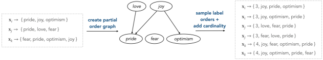
Figure 1: An illustrative task where given an input ${\bm{x}}$, the output is a set of emotions. Our method first discovers a partial order graph (middle) in which specific labels (joy) come before more general labels (pride). Listing the specific labels first gives the model more clues about the rest of the set. Topological samples from this partial order graph are label sequences that can be efficiently generated using seq2seq models. The size of each set is also added as the first element for joint modeling of output with size.

We address these challenges with a novel data augmentation strategy. Specifically, we take advantage of the auto-regressive factorization used by seq2seq models and (i) impose an informative order over the label space, and (ii) explicitly model cardinality. First, the label sets are converted to sequences using informative orders by grouping labels and leveraging their dependency structure. Our method induces a partial order graph over label space where the nodes are the labels, and the edges denote the conditional dependence relations. This graph provides a natural way to obtain informative orders while reinforcing order-invariance. Specifically, sequences obtained via topological traversals of this graph allow independent labels to appear at different locations in the sequence, while restricting order for dependent labels. Next, we jointly model a set with its cardinality by simply prepending the set size to the output sequence. This strategy aligns with the current trend of very large language models which do not lend themselves to architectural modifications but increasingly rely on the informativeness of the inputs (Yang et al., 2020; Liu et al., 2021).

Figure 1 illustrates the key intuitions behind our method using sample task where given an input ${\bm{x}}$ (say a conversation), the output is a set of emotions (${\mathbb{Y}}$). To see why certain orders might be more meaningful, consider a case where one of the emotions is joy, which leads to a more general emotion of pride. After first generating joy, the model can generate pride with certainty (joy leads to pride in all samples). In contrast, the reverse order (generating pride first) still leaves room for multiple possible emotions (joy and love). The order $[\text{joy},\text{pride}]$ is thus more informative than $[\text{pride},\text{joy}]$. The cardinality of a set can also be helpful. In our example, joy contains two sub-emotions, and love contains one. A model that first predicts the number of sub-emotions can be more precise and avoid over-generation, a significant challenge with language generation models (Welleck et al., 2020; Fu et al., 2021). We efficiently sample such informative orders from the combinatorial space of all possible orders and jointly model cardinality by leveraging the auto-regressive nature of seq2seq models.

Our contributions

1. We show an efficient way to model sequence-to-set prediction as a seq2seq task by jointly modeling the cardinality and augmenting the training data with informative sequences using our novel setaug data augmentation approach. (§3.1, 3.2).

2. We theoretically ground our approach: treating the order as a latent variable, we show that our method serves as a better proposal distribution in a variational inference framework. (§3.1)

3. With our approach, seq2seq models of different sizes achieve a $\sim$20% relative improvement on four real-world tasks, with no additional annotations or architecture changes. (§4).

2 Task

We are given a corpus $\mathcal{D}=\{({\bm{x}}_{t},{\mathbb{Y}}_{t})\}_{t=1}^{m}$ where ${\bm{x}}_{t}$ is a sequence of tokens and ${\mathbb{Y}}_{t}=\{{\textnormal{y}}_{1},{\textnormal{y}}_{2},\ldots,{\textnormal{y}}_{k}\}$ is a set. For example, in multi-label fine-grained sentiment classification, ${\bm{x}}_{t}$ is a paragraph, and ${\mathbb{Y}}_{t}$ is a set of sentiments expressed by the paragraph. We use ${\textnormal{y}}_{i}$ to denote an output symbol, $[{\textnormal{y}}_{i},{\textnormal{y}}_{j},{\textnormal{y}}_{k}]$ to denote an ordered sequence of symbols and $\{{\textnormal{y}}_{i},{\textnormal{y}}_{j},{\textnormal{y}}_{k}\}$ to denote a set.

2.1 Set generation using seq2seq model

Task

Given a corpus $\{({\bm{x}}_{t},{\mathbb{Y}}_{t})\}_{t=1}^{m}$, the task of conditional set generation is to efficiently estimate $p({\mathbb{Y}}_{t}\mid{\bm{x}}_{t})$. seq2seq models factorize $p({\mathbb{Y}}_{t}\mid{\bm{x}}_{t})$ autoregressively (ar) using the chain rule:

$$p({\mathbb{Y}}_{t}\mid{\bm{x}}_{t}) =p({\textnormal{y}}_{1},{\textnormal{y}}_{2},\ldots,{\textnormal{y}}_{k}\mid{\bm{x}}_{t})$$

$$=p({\textnormal{y}}_{1}\mid{\bm{x}}_{t})\prod_{j=2}^{k}p({\textnormal{y}}_{j}\mid{\bm{x}}_{i},{\textnormal{y}}_{1}\ldots{\textnormal{y}}_{j-1})$$

where the order ${\mathbb{Y}}_{t}=[{\textnormal{y}}_{1},{\textnormal{y}}_{2},\ldots,{\textnormal{y}}_{k}]$ factorizes the joint distribution using chain rule. In theory, any of the $k!$ orders can be used to factorize the same joint distribution. In practice, the choice of order is important. For instance, Vinyals et al. (2016) show that output order affects language modeling performance when using lstm based seq2seq models for set generation.

Consider an example input-output pair $({\bm{x}}_{t},{\mathbb{Y}}_{t}=\{{\textnormal{y}}_{1},{\textnormal{y}}_{2}\})$. By chain rule, we have the following equivalent factorizations of this sequence: $p({\mathbb{Y}}_{t}\mid{\bm{x}}_{t})=p({\textnormal{y}}_{1}\mid{\bm{x}})p({\textnormal{y}}_{2}\mid{\bm{x}},{\textnormal{y}}_{1})=p({\textnormal{y}}_{2}\mid{\bm{x}})p({\textnormal{y}}_{1}\mid{\bm{x}},{\textnormal{y}}_{2})$. However, order-invariance is only guaranteed with true conditional probabilities, whereas the conditional probabilities used to factorize a sequence are estimated by a model from a corpus. Thus, dependening on the order, the sequence factorizes as either $\hat{p}({\textnormal{y}}_{1}\mid{\bm{x}})\hat{p}({\textnormal{y}}_{2}\mid{\bm{x}},{\textnormal{y}}_{1})$ or $\hat{p}({\textnormal{y}}_{2}\mid{\bm{x}})\hat{p}({\textnormal{y}}_{1}\mid{\bm{x}},{\textnormal{y}}_{2})$, which are not necessarily equivalent. Further, one of these two factorizations may be better represented in the training data, and thus lead to better samples. For instance, if the training data always contains ${\textnormal{y}}_{1},{\textnormal{y}}_{2}$ in the order [${\textnormal{y}}_{1},{\textnormal{y}}_{2}$], $\hat{p}({\textnormal{y}}_{2}\mid{\bm{x}})\hat{p}({\textnormal{y}}_{1}\mid{\bm{x}},{\textnormal{y}}_{2})$ will be $\sim 0$.

Order will also be immaterial if the labels are conditionally independent given the input (Section B.3). However, this assumption is often not valid in practice, especially for nlp, where labels typically share a semantic relationship.

3 Method

This section expands on two critical components of our system, setaug. Section 3.1 presents tsample, a method to create informative orders over sets tractably. Section 3.2 presents our method for jointly modeling cardinality and set output.

3.1 tsample: Adding informative orders for set output

As discussed in Section 2, seq2seq formulation requires the output to be in a sequence. Prior work (Vinyals et al., 2016; Rezatofighi et al., 2018; Chen et al., 2021) has noted that listing the output in orders that have the highest conditional likelihood given the input is an optimal choice. Unlike these methods, we sidestep exhaustive searching during training using our proposed approach tsample.

Our core insight is that knowing the optimal order between pairs of symbols in the output drastically reduces the possible number of permutations. We thus impose pairwise order constraints for labels. Specifically, given an output set ${\mathbb{Y}}_{t}={\textnormal{y}}_{1},{\textnormal{y}}_{2},\ldots,{\textnormal{y}}_{k}$, if ${\textnormal{y}}_{i},{\textnormal{y}}_{j}$ are independent, they can be added in an arbitrary order. Otherwise, an order constraint is added to the order between ${\textnormal{y}}_{i},{\textnormal{y}}_{j}$.

Learning pairwise constraints

We estimate the dependence between elements ${\textnormal{y}}_{i},{\textnormal{y}}_{j}$ using pointwise mutual information: $\texttt{pmi}({\textnormal{y}}_{i},{\textnormal{y}}_{j})=\log p({\textnormal{y}}_{i},{\textnormal{y}}_{j})/p({\textnormal{y}}_{i})p({\textnormal{y}}_{j})$. Here, $\texttt{pmi}({\textnormal{y}}_{i},{\textnormal{y}}_{j})>0$ indicates that the labels ${\textnormal{y}}_{i},{\textnormal{y}}_{j}$ co-occur more than would be expected under the conditions of independence (Wettler and Rapp, 1993). We use $\texttt{pmi}({\textnormal{y}}_{i},{\textnormal{y}}_{j})>\alpha$ to filter our such pairs of dependent pairs, and perform another check to determine if the order between them should be fixed. For each dependent pair ${\textnormal{y}}_{i},{\textnormal{y}}_{j}$, the order is constrained to be $[{\textnormal{y}}_{i},{\textnormal{y}}_{j}]$ (${\textnormal{y}}_{j}$ should come after ${\textnormal{y}}_{i}$) if $\log p({\textnormal{y}}_{j}\mid{\textnormal{y}}_{i})-\log p({\textnormal{y}}_{i}\mid{\textnormal{y}}_{j})>\beta$, and $[{\textnormal{y}}_{j},{\textnormal{y}}_{i}]$ otherwise. Intuitively, $\log p({\textnormal{y}}_{j}\mid{\textnormal{y}}_{i})-\log p({\textnormal{y}}_{i}\mid{\textnormal{y}}_{j})>\beta$ implies that knowledge that a set contains ${\textnormal{y}}_{i}$, increases the probability of ${\textnormal{y}}_{j}$ being present. Thus, in an autoregressive setting, fixing the order to $[{\textnormal{y}}_{i},{\textnormal{y}}_{j}]$ will be more efficient for generating a set with $\{{\textnormal{y}}_{i},{\textnormal{y}}_{j}\}$.

Generating samples

To systematically create sequences that satisfy these constraints, we construct a topological graph $G_{t}$ where each node is a label ${\bm{y}}_{i}\in{\mathbb{Y}}_{t}$, and the edges are determined using the pmi and the conditional probabilities as outlined above (Algorithm 1). The required permutations can then be generated as topological traversals $G_{t}$ (Figure 2). We begin the traversal from a different starting node to generate diverse samples. We call this method tsample. Our method of generating graphs avoids cycles by design (proof in B.4), and thus topological sort remains well-defined. Later, we show that tsample can be interpreted as a proposal distribution in variational inference framework, which distributes the mass uniformly over informative orders constrained by the graph.

Do pairwise constraints hold for longer sequences?

While tsample uses pairwise (and not higher-order) constraints for ordering variables, we note that the pairwise checks remain relevant with extra variables. First, dependence between pair of variables is retained in joint distributions involving more variables (${\textnormal{y}}_{i}\not\perp\!\!\!\perp{\textnormal{y}}_{j}\implies{\textnormal{y}}_{i}\not\perp\!\!\!\perp{\textnormal{y}}_{j},{\bm{y}}_{k}$) for some ${\bm{y}}_{k}\in{\mathbb{Y}}$ (Appendix B.1). Further, if ${\textnormal{y}}_{i},{\textnormal{y}}_{j}\perp\!\!\!\perp{\bm{y}}_{k}$, then it can be shown that $p({\textnormal{y}}_{i}\mid{\textnormal{y}}_{j})>p({\textnormal{y}}_{j}\mid{\textnormal{y}}_{i})\implies p({\textnormal{y}}_{i}\mid{\textnormal{y}}_{j},{\bm{y}}_{k})>p({\textnormal{y}}_{j}\mid{\textnormal{y}}_{i},{\bm{y}}_{k})$ (Appendix B.2). The first property shows that the pairwise dependencies hold in the presence of other set elements. The second property shows that an informative order continues to be informative when additional independent symbols are added. Thus, using pairwise dependencies between the set elements is still effective. Using higher-order dependencies might be suboptimal for practical reasons: higher-order dependencies (or including ${\bm{x}}_{t}$) might not be accurately discovered due to sparsity, and thus cause spurious orders.

Finally, we note that if all the labels are independent, then the order is guaranteed not to matter  (Lemma B.3, also shown empirically in Appendix G). Thus, our method will only be useful when labels have some degree of dependence.

Complexity analysis

Let ${\mathbb{Y}}$ be the label space, $({\bm{x}}_{t},{\mathbb{Y}}_{t})$ be a particular training example, $N$ be the size of the training set, and $c$ be the maximum number of elements for any set ${\mathbb{Y}}_{t}$ in the input. Our method requires three steps: i) iterating over training data to learn conditional probabilities and pmi, and ii) given a ${\mathbb{Y}}_{t}$, building the graph $G_{t}$  (Algorithm 1), and iii) doing topological traversals over $G_{t}$ to create samples for $({\bm{x}}_{t},{\mathbb{Y}}_{t})$.

The time complexity of the first operation is $\mathcal{O}(Nc^{2})$: for each element of the training set, the pairwise count for each pair ${\textnormal{y}}_{i},{\textnormal{y}}_{j}$ and unigram count for each ${\textnormal{y}}_{i}$ is calculated. The pairwise counts can be used for calculating joint probabilities. In principle, we need $\mathcal{O}(|{\mathbb{Y}}|^{2})$ space for storing the joint probabilities. In practice, only a small fraction of the combinations will appear $|{\mathbb{Y}}|^{2}$ in the corpus.

Given a set ${\mathbb{Y}}_{t}$ and the conditional probabilities, the graph $G_{t}$ is created in $\mathcal{O}(c^{2})$ time. Then, generating $k$ samples from $G_{t}$ requires a topological sort, for $\mathcal{O}(kc)$ (or $\mathcal{O}(c)$ per traversal). For training data of size $N$, the total time complexity is $\mathcal{O}(Nck)$. The entire process of building the joint counts and creating graphs and samples takes less than five minutes for all the datasets on an 80-core Intel Xeon Gold 6230 CPU.

Input: Set ${\mathbb{Y}}_{t}$, number of permutations $n$
Parameter: $\alpha,\beta$
Output: $n$ topological sorts over $G_{t}(V,E)$

1:  Let $V={\mathbb{Y}}_{t},E=\emptyset$.

2:  for ${\textnormal{y}}_{i},{\textnormal{y}}_{j}\in{\mathbb{Y}}_{t}$ do

3:     if $pmi({\textnormal{y}}_{i},{\textnormal{y}}_{j})>\alpha$; $\lg p({\textnormal{y}}_{i}\mid{\textnormal{y}}_{j})-\lg p({\textnormal{y}}_{j}\mid{\textnormal{y}}_{i})>\beta$  then

4:        $E=E\cup{\textnormal{y}}_{j}\rightarrow{\textnormal{y}}_{i}$

5:     end if

6:  end for

7:  return $\texttt{topo\_sort}(G_{t}(V,E),n)$

Algorithm 1 Generating permutations for ${\mathbb{Y}}_{t}$

Interpreting tsample as a proposal distribution over orders

We show that our method of augmenting permutations to the training data can be interpreted as an instance of variational inference with the order as a latent variable, and tsample as an instance of a richer proposal distribution.

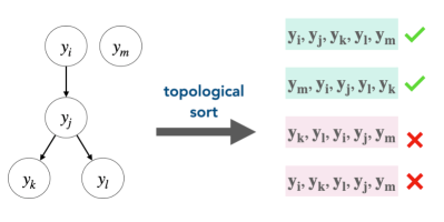
Figure 2: Our sampling method tsample first builds a graph $G_{t}$ over the set ${\mathbb{Y}}_{t}$, and then samples orders from $G_{t}$ using topological sort (topo_sort). The topological sorting rejects samples that do not follow the conditional probability constraints.

Let $\pi_{j}$ be the $j^{th}$ order over ${\mathbb{Y}}_{t}$ (out of $|{\mathbb{Y}}_{t}|!$ possible orders $\Pi$), and $\pi_{j}({\mathbb{Y}}_{t})$ be the sequence of elements in ${\mathbb{Y}}_{t}$ arranged with order $\pi_{j}$. Treating $\pi$ as a latent random variable, the output distribution can then be recovered by marginalizing over all possible orders $\Pi$:

$$\log p_{\theta}({\mathbb{Y}}_{t}\mid{\bm{x}}_{t}) =\log\sum_{\pi_{z}\in\Pi}p_{\theta}(\pi_{z}({\mathbb{Y}}_{t})\mid{\bm{x}}_{t})$$

where $p_{\theta}$ is the seq2seq conditional generation model. While summing over $\Pi$ is intractable, standard techniques from the variational inference framework allow us to write a lower bound (elbo) on the actual likelihood:

$$\log p_{\theta}({\mathbb{Y}}_{t}\mid{\bm{x}}_{t}) =\log\sum_{\pi_{\bm{z}}\in\Pi}p_{\theta}(\pi_{z}({\mathbb{Y}}_{t})\mid{\bm{x}}_{t})$$

$$\geq\underbrace{\mathbb{E}_{q_{\phi}(\pi_{\bm{z}})}\left[\log\frac{p_{\theta}(\pi_{\bm{z}}({\mathbb{Y}}_{t})\mid{\bm{x}}_{t})}{q_{\phi}(\pi_{\bm{z}})}\right]}_{\textsc{elbo}}=\mathcal{L}(\theta,\phi)$$

In practice, the optimization procedure draws $k$ samples from the proposal distribution $q$ to optimize a weighted elbo (Burda et al., 2016; Domke and Sheldon, 2018). Crucially, $q$ can be fixed (e.g., to uniform distribution over the orders), and in such cases only $\theta$ are learned (Appendix H). The data augmentation approach used for xl-net (Yang et al., 2019b) can be interpreted with this framework. In their case, the proposal distribution $q$ is fixed to a uniform distribution for generating orders over tokens. The variational interpretation also indicates that it might be possible to improve language modeling by using a different, more informative $q$. Investigating such proposal distribution for language modeling is an interesting future work.

tsample can thus be seen as a particular proposal distribution that assigns all the support to the topological ordering over the label dependence graphs. We experiment with sampling from a uniform distribution over the samples (referred to as random experiments in our baseline setup). The idea of using an informative proposal distribution over space of structures to do variational inference has also been used in the context of grammar induction (Dyer et al., 2016) and graph generation (Jin et al., 2018; Chen et al., 2021). Our formulation is closest in spirit to Chen et al. (2021). However, the set of nodes to be ordered is already given in their graph generation setting. In contrast, we infer the order and the set elements jointly from the input.

3.2 Modeling cardinality

Let $m=|{\mathbb{Y}}_{t}|$ be the cardinality (number of elements) in ${\mathbb{Y}}_{t}$. Our goal is to jointly estimate $m$ and ${\mathbb{Y}}_{t}$ (i.e., $p(m,{\mathbb{Y}}_{t}\mid{\bm{x}}_{t})$). Additionally, we want the model to use the cardinality information for generating ${\mathbb{Y}}_{t}$. We add the cardinality information at the beginning of the sequence, thus converting a sample $({\bm{x}}_{t},{\mathbb{Y}}_{t})$ to $({\bm{x}}_{t},[|{\mathbb{Y}}_{t}|,\pi({\mathbb{Y}}_{t})])$, and then train our seq2seq model as usual from ${\bm{x}}\rightarrow[|{\mathbb{Y}}_{t}|,\pi({\mathbb{Y}}_{t})]$. Here $\pi$ is some ordering that converts the set ${\mathbb{Y}}_{t}$ to a sequence. As seq2seq models use autoregressive factorization, listing the order information first ensures that the distribution $p([|{\mathbb{Y}}_{t}|,\pi({\mathbb{Y}}_{t})]\mid{\bm{x}}_{t})$ factorizes as $p([|{\mathbb{Y}}_{t}|,\pi({\mathbb{Y}}_{t})]\mid{\bm{x}}_{t})=p(|{\mathbb{Y}}_{t}|\mid{\bm{x}}_{t})p(\pi({\mathbb{Y}}_{t})\mid|{\mathbb{Y}}_{t}|,{\bm{x}}_{t})$. Thus, the generation of ${\mathbb{Y}}_{t}$ is conditioned on the input and the cardinality $|{\mathbb{Y}}_{t}|$ (due to $p(\pi({\mathbb{Y}}_{t})\mid|{\mathbb{Y}}_{t}|,{\bm{x}}_{t})$ term).

Why should cardinality help?

Unlike models like deep sets (Zhang et al., 2019a), seq2seq models are not restricted by the number of elements generated. However, adding cardinality information has two potential benefits: i) it can help avoid over-generation (Welleck et al., 2020; Fu et al., 2021), and ii) unlike free-form text output, the distribution of the set output size ($p(|{\mathbb{Y}}_{t}|\mid{\bm{x}}_{t})$) might benefit the model to adhere to the set size constraint. Thus, information on the predicted size can be beneficial for the model to predict the elements to be generated.

4 Experiments

setaug comprises: i) tsample, a way to generate informative orders to convert sets to sequences, and ii) card: jointly modeling cardinality and the set output. This section answers two questions:

• How well does setaug improve existing models? Specifically, how well setaug can take an existing seq2seq model and improve it just using our data augmentation and joint cardinality prediction, without making any changes to the model architecture. We also measure if these performance improvements carry across diverse datasets, model classes, and inference settings.

• Why does our approach improve performance? We study the contributions of tsample and joint cardinality prediction (card), and analyze where setaug works or fails.

4.1 Setup

Tasks

We consider multi-label classification and keyphrase generation. These tasks represent set generation problems where the label space spans a set of fixed categories (multi-label classification) or free-form phrases (keyphrase generation).

1. Multi-label classification task: We have three datasets of varying sizes and label space:

• Go-Emotions classification (go-emo, Demszky et al. (2020)): generate a set of emotions for a paragraph.

• Open Entity Typing (openent, Choi et al. (2018)): assigning open types (free-form phrases) to the tagged entities in the input text.

• Reuters-21578 (reuters, Lewis (1997)): labeling news article with the set of mentioned economic subjects.

2. Keyphrase generation (keygen): We experiment with a popular keyphrase generation dataset, KP20K (Meng et al., 2017) which involves generating keyphrases for a scientific paper abstract.

Table 1 lists the dataset statistics and examples from each dataset are shown in Appendix E. We treat all the problems as open-ended generation, and do not use any specialized pre-processing. For all the datasets, we filter out samples with a single label. For each training sample, we create $n$ permutations using setaug.

Baselines

We compare with two baselines:
i) multi-label: As a non-seq2seq baseline, we train a multi-label classifier that makes independent predictions of the output labels. Encoder-only and encoder-decoder approaches can be adapted for multi-label, and we experiment with bart (encoder-decoder) and bert (encoder-only). This baseline represents a standard method for doing multi-label classification (e.g., Demszky et al. (2020)). During inference, top-k logits are returned as the predicted set. We search over $k=[1,3,5,10,50]$ and use $k$ that performs the best on the dev set. Table 13 in Appendix F shows precision, recall, and $F$ scores at each-k.

ii) set search: each training sample $({\bm{x}},\{{\textnormal{y}}_{1},{\textnormal{y}}_{2},\ldots,{\textnormal{y}}_{k}\})$ is converted into $k$ training examples $\{({\bm{x}},{\textnormal{y}}_{i})\}_{i=1}^{k}$. We fine-tune bart-base to generate one training sample for input ${\bm{x}}$. During inference, we run beam-search with the maximum set size in the training data (Table 1). The unique elements generated by beam search are returned as the set output, a popular approach for one-to-many generation tasks (Hwang et al., 2021).

setaug can apply to any seq2seq model. We show results with models of various capacity:

• bart-base (Lewis et al., 2020) (110M),

• t5-11b (Raffel et al., 2020) (11B), and

• gpt3-175b (Brown et al., 2020) (175B).

Task	Avg/min/max labels per sample	Unique labels	Train/test/dev samples per split
go-emo	3.03/3/5	28	0.6k/0.1k/0.1k
openent	5.4/2/18	2519	2k/2k/2k
reuters	2.52/2/11	90	0.9k/0.4k/0.3k
keygen	3.87/3/79	274k	156k/2k/2k

Table 1: Datasets used in our experiments.

Training

We augment $n=2$ permutations to the original data using tsample. For all the results, we use three epochs and the same number of training samples (i.e., input data for the baselines is oversampled). This controls for models trained with augmented data improving only because of factors such as longer training time. All the experiments were repeated for three different random seeds, and we report the averages. We found from our experiments that hyperparameter tuning over $\alpha,\beta$ did not affect the results in any significant way. For all the experiments reported, we use $\alpha=1$ and $\beta=\log_{2}(3)$. We use a single GeForce RTX 2080 Ti for all our experiments on bart, and a single TPU for all experiments done with T5-11B. For gpt3-175b, we use the OpenAI completion engine (davinci) API (OpenAI, 2021). Additional hyperparameter details in Appendix D. We use greedy sampling for all experiments. Our method remains effective across five different sampling techniques, incl. beam search, nucleus, top-k, and random sampling (Table 14, Appendix G).

4.2 setaug improves existing models

Our method helps across a wide range of models (bart, t5-11b, and gpt3-175b) and tasks.

4.2.1 Multi-label classification

Table 2 shows improvements across all datasets and models for the multi-label classification task ($\sim$20% relative gains). For brevity, we list macro $F$ score, and include detailed results including macro/micro precision, recall, $F$ scores in Table 9 (Appendix F). We attribute the comparatively lower performance of set search baseline to two specific reasons - repeated generation of the same set of terms (e.g., person, business for openent) and generating elements not present in the test set (see Section 4.3.4 for a detailed error analysis). We see similar trends with gpt3-175b (Section 4.2.4).

	go-emo	openent	reuters
set search (bart)	7.4	26.3	7.5
multi-label (bart)	25.6	16.4	25.2
multi-label (bert)	25.7	16.2	25.5
bart	23.4	44.6	15.6
bart + setaug	30.0	53.5	26.7
t5-11b	47.8	53.6	45.3
t5-11b + setaug	50.9	57.0	48.5

Table 2: setaug improves seq2seq models by $\sim$20% relative $F1$- points, on three multilabel classification datasets. bart and t5-11b are trained on the original datasets with a random order and no cardinality. “+ setaug” indicates augmented train data using tsample and cardinality is prepended to the output sequence.

Ye et al. (2021)	bart	bart + setaug
5.8	5.3	6.5
39.2	36.3	39.1

Table 3: setaug improves off-the-shelf bart-base for keyphrase generation task

4.2.2 Keyphrase generation

To further motivate the utility of seq2seq models for set generation tasks, we experiment on KP-20k, which is an extreme multi-label classification dataset (Meng et al., 2017) with label space spanning over 257k unique keyphrases. Due to the large label space, training multi-class classification baselines is not computationally viable. In this dataset, the input text is an abstract from a scientific paper. We use the splits used by Ye et al. (2021). For a fair comparison with Ye et al. (2021), we use bart-base for this experiment. Table 3 shows the results. Similar to datasets with smaller label space, our method improves on vanilla seq2seq.

We want to emphasize that while specialized models for individual tasks might be possible, we aim to propose a general approach that shows that sampling informative orders can help efficient and general set-generation modeling.

4.2.3 Simulations

Following prior work on studying deep network properties effectively via simulation (Vinyals et al., 2016; Khandelwal et al., 2018), we design a simulation to study the effects of output order and cardinality on conditional set generation. The simulation reveals several key properties of our methods. We defer the details to Appendix G, and mention some key findings here. We find similar trends in simulated settings. Specifically, our method is (i) ineffective when labels are independent, (ii) helpful even when position embeddings are disabled, and (iii) helps across a wide range of sampling types.

4.2.4 Few-shot prompting with gpt3-175b

We fine-tune the generation models using augmented data for both bart and t5-11b. However, fine-tuning models at the scale of gpt3-175b is prohibitively expensive. Thus such models are typically used in a few-shot prompting setup. In a few-shot prompting setup, $M$ ($\sim$10-100) input-output examples are selected as a prompt $p$. A new input $x$ is appended to the prompt $p$, and $p\|x$ is the input to gpt3-175b. Improving these prompts, sometimes referred to with an umbrella term prompt tuning (Liu et al., 2021), is a popular and emergent area of nlp. Our approach is the only feasible candidate for such settings, as it does not involve changing the model or additional post-processing. We apply our approach for tuning prompts for generating sets in few-shot settings. We focus on go-emo and openent tasks, as the relatively short input examples allow cost-effective experiments. We randomly create a prompt with $M=24$ examples from the training set and run inference over the test set for each. For each example in the prompt, we order the set of emotions using our ordering approach tsample and compare the results with random orderings. Using tsample to arrange the labels outperforms random ordering for both openent (macro $F$ 34 vs. 39.5 with ours, 15% statistically significant relative improvement), and go-emo (macro $F$ 16.5 vs. 14.5, 14% relative improvement). This suggests that ordering helps performance in resource-constrained settings e.g., few-shot prompting.

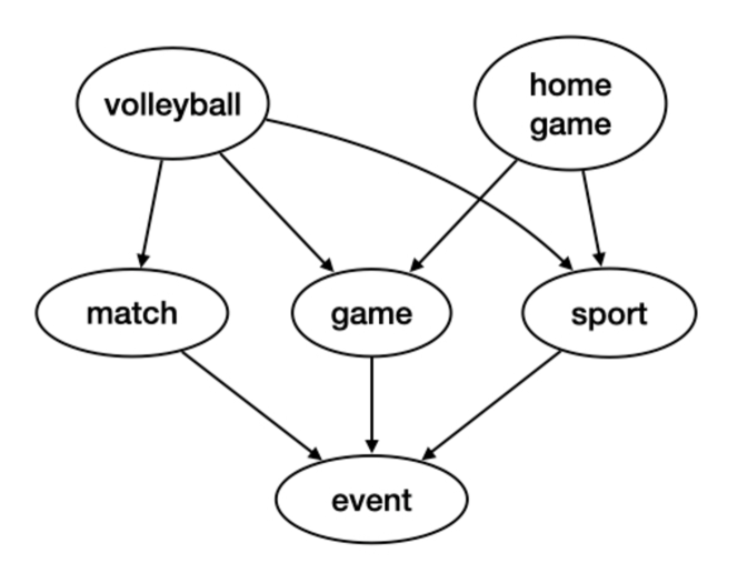
Figure 3: Label dependency discovered by tsample for openent: specific entities (e.g., volleyball) precede generic ones (event). Appendix C has more examples

4.3 Why does setaug improve performance?

As mentioned in Section 3, our method of generating sets with seq2seq models consists of two components: i) a strategy for sampling informative orders over label space (tsample), and ii) jointly generating cardinality of the output (card). This section studies the individual contributions of these components in order to answer RQ2.

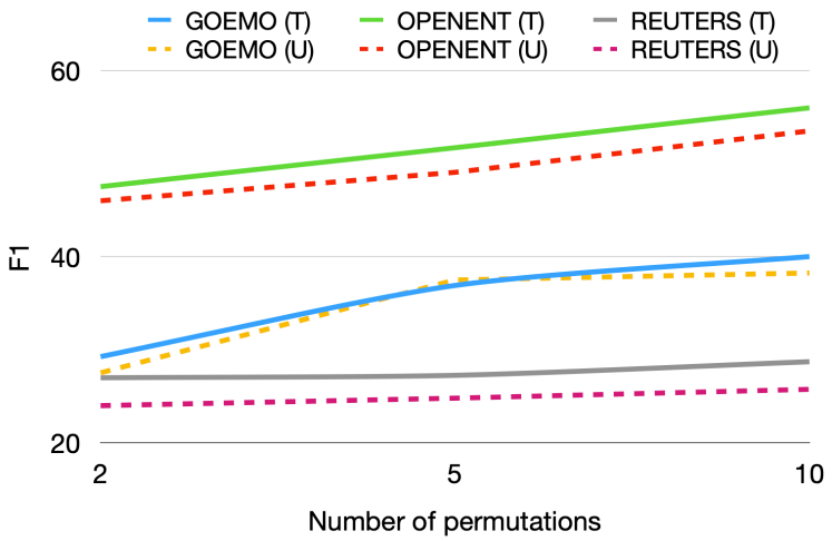
Figure 4: setaug (T) consistently outperforms random (U) as the number of permutations ($n$) is increased.

4.3.1 Ablation study

We ablate the two critical components of our system: cardinality (setaug- card) and order (setaug- tsample) and investigate the performance for each of these settings using bart for multi-label classification. Table 4 presents the results. Both the components individually help, but a larger drop is seen by removing cardinality. We also train using random orders, instead of tsample. random does not improve over seq2seq consistently (both with and without card), showing that merely augmenting with random permutations does not help. Further, Appendix F shows that cardinality is useful even with random order.

	go-emo	openent	reuters
setaug	30.0	53.5	26.7
- card	23.3 (-22%)	48.0 (-10%)	15.8 (-40%)
- tsample	26.8 (-11%)	50.5 (-6%)	24.3 (-9%)
random	27.5 (-8%)	50.4 (-6%)	24.7 (-7%)
freq	19.03 (-36%)	49.9 (-7%)	23.4 (-12%)

Table 4: Ablations: modeling cardinality (card) and sampling informative orders (tsample) both help, with larger gains from card. random ordering hurts.

4.3.2 Role of order

Nature of permutations created by setaug

setaug encourages highly co-occurring pairs (${\textnormal{y}}_{i},{\textnormal{y}}_{j}$) to be in the order ${\textnormal{y}}_{i},{\textnormal{y}}_{j}$ if $p({\textnormal{y}}_{j}\mid{\textnormal{y}}_{i})>p({\textnormal{y}}_{i}\mid{\textnormal{y}}_{j})$. In our analysis, this dependency in the datasets shows that the orders exhibit a pattern where specific labels appear before the generic ones. E.g., in entity typing, the more generic entity event is generated after the more specific entities home game and match (see Figure 3).

Increasing # permutations ($n$) helps:

Fig. 4 shows that setaug and random improve as $n$ is increased from $n=2$ to $10$; setaug outperforms random across $n$.

Reversing the order hurts performance

In order to check our hypothesis of whether only informative orders helping with set generation, we invert the label dependencies returned by setaug for all the datasets and train with the same model settings. Across all datasets, we observe that reversing the order leads to an average of 12% drop in $F1$- score. The reversed order not only closes the gap between setaug and random, but in many instances, the performance is slightly worse than random.

Ordering by frequency

Yang et al. (2018) use frequency ordering, where the most frequent label is placed first in the sequence. We compare with this baseline in Table 4 (freq). The results indicate that the performance of frequency-based ordering is dataset dependent. Relying on a fixed criteria like frequency might lead to skewed outputs, especially for datasets with a long-tail of labels. For instance, for openent, one of the most significant failure modes of the freq method was generating the most common label in the corpus (person) for every input. TSAMPLE can be seen as a way to balance the most frequent and least frequent labels in the corpus using pmi and conditional likelihood (Algorithm 1, L3).

4.3.3 Role of cardinality

Cardinality is successfully predicted and used

Table 4 shows that cardinality is crucial to modeling set output. To study whether the models learn to condition on predicted cardinality, we compute an agreement score - defined as the % of times the predicted cardinality matches the number of elements generated by the model. The model effectively predicts the cardinality almost exactly in go-emo and reuters datasets (avg. 95%). While the exact match agreement is low in openent (35%), the model is within an error of $\pm$1 in 93% of the cases. These results show that cardinality predicts the end of sequence (eos) token. The accuracy for predicting the exact cardinality is 61% across datasets, and it increases to 76% within an error of 1 (i.e., when the predicted cardinality is off by 1).

Information about cardinality improves multi-label classification

multi-label baseline uses different values of k for predicting labels. To test if knowledge of cardinality improves multi-class classification, we experiment with a setting where the true cardinality is available at inference (i.e., $k$ is set to the true value of cardinality). Table 5 shows that cardinality improves performance.

	go-emo	openent	reuters
multi-label	22.4	14.3	21.7
multi-label-k*	21.3(-4.9%)	17.8(+24.5%)	25.6(+18%)

Table 5: Cardinality improves multi-label classification.

4.3.4 Error analysis

We manually compare the outputs generated by the vanilla bart model with bart + setaug. For the open-entity typing dataset, we randomly sample 100 examples and find that vanilla seq2seq approach generates sets with an ill-formed element 22% of the time, whereas setaug completely avoids this. Examples of such ill-formed elements include personformer, businessirm, polit, foundationirm, politplomat, eventlete. This analysis indicates that training the model with an informative order infuses more information about the underlying type-hierarchy, avoiding the ill-formed elements.

5 Related work

Set generation in nlp

Prior work has noted the impact of the order on the performance of text generation models (Vinyals et al., 2016), especially in the context of keyphrase generation (Meng et al., 2019). Approaches to explicitly model set properties for NLP tasks include either performing an exhaustive search to find the best order (Vinyals et al., 2016), changing the model training to modify the loss function (Qin et al., 2019), or applying post-processing (Nag Chowdhury et al., 2016). Notably, Ye et al. (2021) introduced One2Set, a method for training order-invariant models for generating set of keyphrases. Our main goal in this work is to provide a framework to identify useful orders for set generation, and show that such orders can help vanilla seq2seq models. setaug can work with any seq2seq model, and is complementary to these specialized methods.

Non-seq2seq set generation

These include reinforcement learning for multi-label classification (Yang et al., 2019a) and combinatorial problems (Nandwani et al., 2020), and using pointer networks for keyphrase extraction (Ye et al., 2021). We focus on optimally adapting existing seq2seq models for set generation, without external knowledge (Wang et al., 2021; Zhang et al., 2019b).

Chen et al. (2021) explored the generation of an optimal order for graph generation given the nodes. They observed that ordering nodes before inducing edges improves graph generation. However, in our case, since the labels are unknown, conditioning on the labels to create the optimal order is not possible.

Connection with Janossy pooling

Murphy et al. (2019) generalize deep sets by encoding a set of $N$ elements by pooling permutations of $P(N,k)$ tuples. With $k=N$, their method is the same as pooling all $N!$ sequences, and reduces to deep sets with $k=1$. We share similarity with tractable searching over $N!$ with Janossy pooling, but instead of iterating over all possible 2-tuples, we impose pairwise constraints on the element order.

Modeling set input

A number of techniques have been proposed for encoding set-shaped inputs (Santoro et al., 2017; Zaheer et al., 2017; Lee et al., 2019; Murphy et al., 2019; Huang et al., 2020; Kim et al., 2021). Specifically, Zaheer et al. (2017) propose deep sets, wherein they show that pooling the representations of individual set elements and feeding the resulting features to a non-linear network is a principled way of representing sets. Lee et al. (2019) present permutation-invariant attention to encode shapes and images using a modified version of attention (Vaswani et al., 2017). Unlike these works, we focus on settings where the input is a sequence, and the output is a set.

6 Conclusion and Discussion

We present setaug, a novel data augmentation method for conditional set generation that incorporates informative orders and adds cardinality information. Our key idea is using the most likely order (vs. a randomly selected order) to represent a set as a sequence and conditioning the generation of a set on predicted cardinality. As a computationally efficient and general-purpose plug-in data augmentation algorithm, setaug improves seq2seq models for set generation across a wide spectrum of tasks. For future work, it would be interesting to investigate if the general ideas in this work have applications in settings beyond set generation. Examples include generating additional data to improve language modeling in low-resource scenarios and determining the ideal order of in-context examples in a prompt.

Limitations

Ineffectiveness on independent sets

setaug is only useful when the labels share some degree of dependence. For tasks where the labels are completely independent, setaug will not be effective. It can be shown that order will not affect learning joint distribution over labels if the labels are independent (Lemma B.3). Thus, in such settings, any method (including setaug) that seeks to leverage the relationship between labels will not be helpful. In addition to Lemma B.3, we conduct thorough simulation studies to verify this limitation (Figure 8).

Use of large language models

We perform experiments with extremely large models, including T5-XXL and GPT-3 models. Particularly, GPT-3 is only available through OpenAI API; thus, all the details about its working are not publicly available. However, our experiments also show results using BART models that run on a single RTX 2080 GPU (please also see details on reproducibility in Appendix A). Further, such language models are typically trained on a large English corpora, which is also the focus of our work.

Focus on seq2seq

A key limitation of our work is that it focuses on set-generation using seq2seq models. Thus the proposed insights may not apply to other settings (e.g., computer vision) where using language models is not directly feasible. Nevertheless, with the growing popularity of libraries like Huggingface (Wolf et al., 2019), we anticipate that seq2seq models will be applied to a growing number of use cases, even those that would traditionally be tackled using a non-seq2seq method. Further, we compare our method with representative non-seq2seq baselines (like multi-label classifier).

To our knowledge, our work does not directly use any datasets that contain explicit societal biases. Therefore, we anticipate that our work will not lead to any significant negative implications concerning real-world applications.

Appendix A Reproducibility

We take the following steps for reproducibility of our results:

1. All the experiments are performed for three different random seeds. In addition, we conduct a proportion of samples hypothesis test to establish the statistical significance of our results. We did not perform extensive hyperparameter tuning and used the same set of defaults for baselines and our proposed method.

2. For all data augmentation experiments, we match the number of training samples and epochs; all the models are trained for the same duration. This alleviates the concern that the models perform well with augmented data merely because of the longer training time.

3. We conduct a proportion of samples test for all the experiments conducted on real-world datasets and use a small $p=0.0005$ to measure highly significant results, which are indicated with an underscore.

Our work aims to promote the usage of existing resources for as many use cases as possible. In particular, all our experiments are performed on the BASE-version of the model (BART) that can relatively lower parameter count to conserve resources and help lower our impact on climate change.

Appendix B Proofs

Let ${\mathbb{Y}}$ be the output space, ${\textnormal{y}}_{i},{\textnormal{y}}_{j},{\textnormal{y}}_{k}\in{\mathbb{Y}}$, and ${\bm{y}}_{k}\in{\mathbb{Y}}-{\textnormal{y}}_{i}-{\textnormal{y}}_{j}$ be a subset of the symbols excluding ${\textnormal{y}}_{i},{\textnormal{y}}_{j}$. We assume that all the distributions are non-negative (i.e., $p({\bm{y}})>0,\forall{\bm{y}}\in{\mathbb{Y}}$)

Lemma B.1.

${\textnormal{y}}_{i}\not\perp\!\!\!\perp{\textnormal{y}}_{j}\implies{\textnormal{y}}_{i}\not\perp\!\!\!\perp({\textnormal{y}}_{j}{\textnormal{y}}_{k})$

Proof

Let ${\textnormal{y}}_{i}\perp\!\!\!\perp({\textnormal{y}}_{j}{\textnormal{y}}_{k})$ by contradiction. Then:

$$p({\textnormal{y}}_{i},{\textnormal{y}}_{j}{\textnormal{y}}_{k}) =p({\textnormal{y}}_{i})p({\textnormal{y}}_{j}{\textnormal{y}}_{k})$$ (1)

Also,

$$p({\textnormal{y}}_{i},{\textnormal{y}}_{j}) =\sum_{{\textnormal{y}}_{k}\in{\bm{Z}}}p({\textnormal{y}}_{i},{\textnormal{y}}_{j}{\textnormal{y}}_{k})$$

$$=\sum_{{\textnormal{y}}_{k}\in{\bm{Z}}}p({\textnormal{y}}_{i})p({\textnormal{y}}_{j}{\textnormal{y}}_{k})$$ (equation 1)

$$=p({\textnormal{y}}_{i})\sum_{{\textnormal{y}}_{k}\in{\bm{Z}}}p({\textnormal{y}}_{j}{\textnormal{y}}_{k})$$

$$=p({\textnormal{y}}_{i})p({\textnormal{y}}_{j})$$ (2)

However, ${\textnormal{y}}_{i}\not\perp\!\!\!\perp{\textnormal{y}}$ thus ${\textnormal{y}}_{i}\not\perp\!\!\!\perp{\textnormal{y}}\implies{\textnormal{y}}_{i}\not\perp\!\!\!\perp({\textnormal{y}}_{j}{\textnormal{y}}_{k})$.

Lemma B.2.

$$p({\textnormal{y}}_{i}\mid{\textnormal{y}}_{j})>p({\textnormal{y}}_{j}\mid{\textnormal{y}}_{i})\implies p({\textnormal{y}}_{i}\mid{\textnormal{y}}_{j},{\bm{y}}_{k})>p({\textnormal{y}}_{j}\mid{\textnormal{y}}_{i},{\bm{y}}_{k})$$

if ${\textnormal{y}}_{i},{\textnormal{y}}_{j}\perp\!\!\!\perp{\bm{y}}_{k}$

Proof

We have:

$$p({\textnormal{y}}_{i}\mid{\textnormal{y}}_{j}) >p({\textnormal{y}}_{j}\mid{\textnormal{y}}_{i})$$

$$\implies p({\textnormal{y}}_{j}) <p({\textnormal{y}}_{i})$$ (3)

$$p({\textnormal{y}}_{j},{\bm{y}}_{k}) =p({\bm{y}}_{k}\mid{\textnormal{y}}_{j})p({\textnormal{y}}_{j})$$

$$<p({\bm{y}}_{k}\mid{\textnormal{y}}_{j})p({\textnormal{y}}_{i})$$

$$=p({\bm{y}}_{k}\mid{\textnormal{y}}_{i})p({\textnormal{y}}_{i}) {\textnormal{y}}_{i},{\textnormal{y}}_{j}\perp\!\!\!\perp{\bm{y}}_{k}\implies p({\bm{y}}_{k}\mid{\textnormal{y}}_{j})=p({\bm{y}}_{k}\mid{\textnormal{y}}_{i})=p({\bm{y}}_{k})$$ ()

$$=p({\textnormal{y}}_{i},{\bm{y}}_{k})$$ (4)

Thus,

$$p({\textnormal{y}}_{i}\mid{\textnormal{y}}_{j},{\bm{y}}_{k}) =\frac{p({\textnormal{y}}_{i},{\textnormal{y}}_{j},{\bm{y}}_{k})}{p({\textnormal{y}}_{j},{\bm{y}}_{k})}$$

$$>\frac{p({\textnormal{y}}_{i},{\textnormal{y}}_{j},{\bm{y}}_{k})}{p({\textnormal{y}}_{i},{\bm{y}}_{k})}$$

$$=p({\textnormal{y}}_{j}\mid{\textnormal{y}}_{i},{\bm{y}}_{k})$$ (5)

Lemma B.3.

If ${\textnormal{y}}_{i}\perp\!\!\!\perp{\textnormal{y}}_{j}\ \forall{\textnormal{y}}_{i},{\textnormal{y}}_{j}\in{\mathbb{Y}}$, the order is guaranteed to not affect learning.

Proof

Let $\pi_{j}$ be the $j^{th}$ order over ${\mathbb{Y}}$ (out of $|{\mathbb{Y}}|!$ possible orders $\Pi$), and $\pi_{j}({\mathbb{Y}})$ be the sequence of elements in ${\mathbb{Y}}$ arranged with $\pi_{j}$.

$$p({\textnormal{y}}_{i}\mid{\textnormal{y}}_{j}) =p({\textnormal{y}}_{i}) {\textnormal{y}}_{i}\perp\!\!\!\perp{\textnormal{y}}_{j}\ \forall{\textnormal{y}}_{i},{\textnormal{y}}_{j}$$ ()

$$\implies p({\textnormal{y}}_{i},{\textnormal{y}}_{j},{\textnormal{y}}_{k}) =p({\textnormal{y}}_{i})p({\textnormal{y}}_{j}\mid{\textnormal{y}}_{i})p({\textnormal{y}}_{k}\mid{\textnormal{y}}_{i},{\textnormal{y}}_{j})$$

$$=p({\textnormal{y}}_{i})p({\textnormal{y}}_{j})p({\textnormal{y}}_{k})$$

$$\implies p(\pi_{m}({\textnormal{y}}_{i},{\textnormal{y}}_{j},{\textnormal{y}}_{k})) =p(\pi_{n}({\textnormal{y}}_{i},{\textnormal{y}}_{j},{\textnormal{y}}_{k}))\ \forall\pi_{m},\pi_{m}\in\Pi$$

In other words, when all elements are mutually independent, all possible joint factorizations will simply be a product of the marginals, and thus identical.

Lemma B.4.

The graphs constructed to sample orders for setaug cannot have cycles.

Proof

Let ${\textnormal{y}}_{i},{\textnormal{y}}_{j},{\textnormal{y}}_{k}$ form a cycle: ${\textnormal{y}}_{i}\rightarrow{\textnormal{y}}_{j}\rightarrow{\textnormal{y}}_{k}\rightarrow{\textnormal{y}}_{i}$. By construction, the following conditions must hold for such a cycle to be present:

$$\log p({\textnormal{y}}_{j}\mid{\textnormal{y}}_{i})-\log p({\textnormal{y}}_{i}\mid{\textnormal{y}}_{j}) >\beta\implies\log p({\textnormal{y}}_{i})<\log p({\textnormal{y}}_{j})$$

$$\log p({\textnormal{y}}_{k}\mid{\textnormal{y}}_{j})-\log p({\textnormal{y}}_{j}\mid{\textnormal{y}}_{k}) >\beta\implies\log p({\textnormal{y}}_{j})<\log p({\textnormal{y}}_{k})$$

$$\log p({\textnormal{y}}_{i}\mid{\textnormal{y}}_{k})-\log p({\textnormal{y}}_{k}\mid{\textnormal{y}}_{i}) >\beta\implies\log p({\textnormal{y}}_{k})<\log p({\textnormal{y}}_{i})$$

Putting the three implications together, we get $\log p({\textnormal{y}}_{i})<\log p({\textnormal{y}}_{j})<\log p({\textnormal{y}}_{k})<\log p({\textnormal{y}}_{i})$, which is a contradiction. Hence, the graphs constructed for setaug cannot have a cycle.

Appendix C Sample graphs

In this section, we present additional examples from reuters and go-emo datasets to illustrate the permutations generated by our method. As discussed in Section 3.1, setaug encourages highly co-occuring pairs (${\textnormal{y}}_{i},{\textnormal{y}}_{j}$) to be in the order ${\textnormal{y}}_{i},{\textnormal{y}}_{j}$ if $p({\textnormal{y}}_{j}\mid{\textnormal{y}}_{i})>p({\textnormal{y}}_{i}\mid{\textnormal{y}}_{j})$. In our analysis, this dependency in the datasets shows that the orders exhibit a pattern where specific labels appear before the generic ones. For example, in case of entity typing, the more go-emo, sadness is generated after the more specific emotion remorse and fear (Figure 5). Similarly, the entity crude is generated after the entities gas and nat-gas. (Figure 6 (right)).

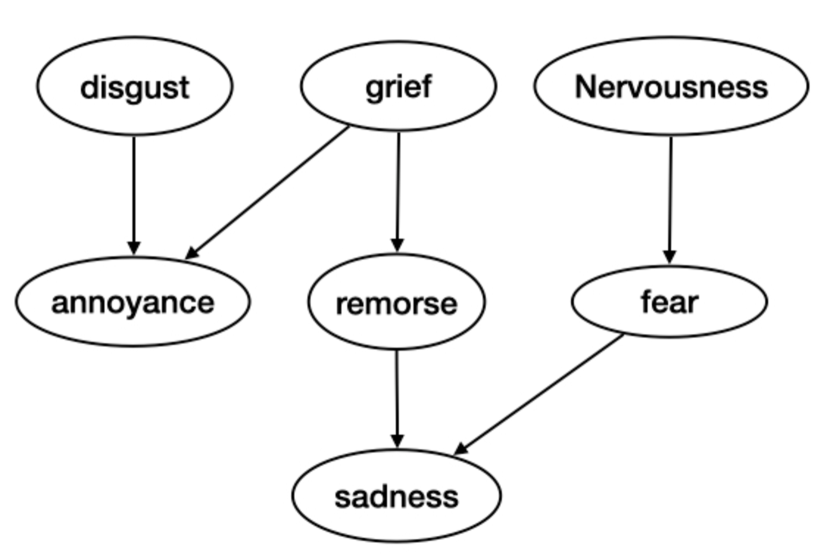
Figure 5: Label dependencies discovered by tsample for go-emo

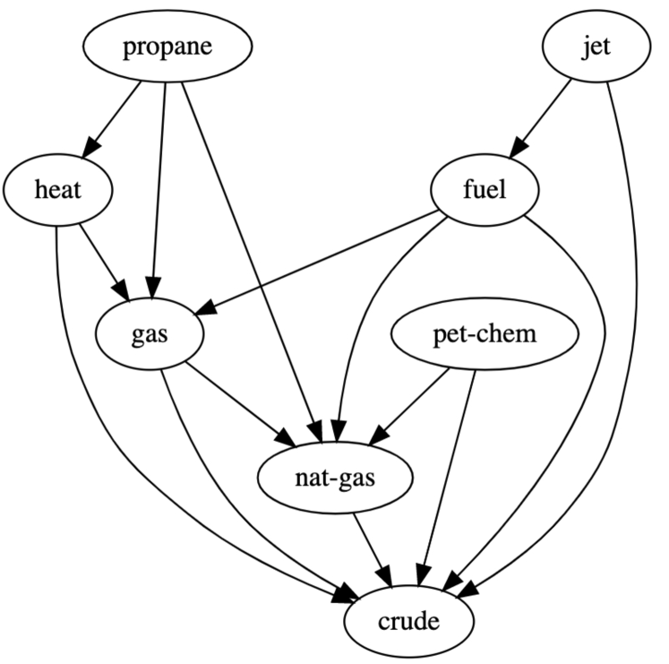
Figure 6: Label dependencies discovered by tsample for reuters

Appendix D Hyperparameters

We list all the hyperparameters in Table 6.

Hyperparameter	Value
GPU	GeForce RTX 2080 Ti
gpus	1
auto_select_gpus	false
accumulate_grad_batches	1
max_epochs	3
precision	32
learning_rate	1e-05
adam_epsilon	1e-08
num_workers	16
warmup_prop	0.1
seeds	[15143, 27122, 999888]
add_lr_scheduler	true
lr_scheduler	linear
max_source_length	120
max_target_length	120
val_max_target_length	120
test_max_target_length	120

Table 6: List of hyperparameters used for all the experiments.

Appendix E Dataset

Table 7 shows examples for each of the datasets.

	Input	Output
Fine-grained emotion classification, [28] (Demszky et al., 2020)	So there’s hope for the rest of us! Thanks for sharing. What helped you get to where you are?	{curiosity, gratitude, optimism}
Open-entity typing [2519]
(Choi et al., 2018)	Some 700,000 cubic meters of caustic sludge and water burst inundating $[\text{SPAN}]$ three west Hungarian villages $[\text{SPAN}]$ and spilling.	{colony, region, location, hamlet, area, village, settlement, community}
Reuters [90]
(Lewis, 1997)	India is reported to have bought two white sugar cargoes for$\ldots$ $\ldots$cargo sale, they said.	{ship, sugar}
Keyphrase generation [270k]
(Ye et al., 2021)	We analyze the impact of core affinity on both network and disk i/o performance…our dynamic core affinity improves the file upload throughput more than digit%	{big data, multi-core, process-scheduling}

Table 7: Real world tasks used for experiments

Appendix F Additional results

This section presents detailed results that were omitted from the main paper for brevity. This includes macro and micro precision, recall, and $F$ scores on all datasets, and additional ablation experiments.

1. Table 9 shows the detailed results from the four tasks.

2. Detailed results on go-emo, reuters, and openent are present in Tables 12, 12, and 12, respectively.

3. Table 13 includes results from a multi-label classification baseline where bert-base-uncased is used as the encoder.

	go-emo	openent	reuters
multi-label	22.4	14.3	21.7
multi-label @oracle-k	21.3	17.8	25.6
setaug + card	30.0	53.5	26.7

Table 8: Multi-label classification when the true cardinality is provided to the classifier. While providing the true cardinality helps the performance of multi-label classifiers, it still lags setaug.

	go-emo			openent			reuters			keygen
	$p$	$r$	$F$	$p$	$r$	$F$	$p$	$r$	$F$	$p$	$r$	$F$
multi-label	20.8	42.4	22.4	16.4	25.1	14.3	19.7	43.4	21.7	-	-	-
multi-label-k*	21.3	21.3	21.3	17.8	17.8	17.8	25.6	25.6	25.6	-	-	-
set search	10.7	7.0	7.4	26.5	31.4	26.3	10.9	7.1	7.5	5.8	7.4	6.4
seq2seq	27.4	26.2	23.4	55.4	42.4	44.6	24.8	13.8	15.6	6.7	5.5	5.9
random	32.5	19.9	22.7	62.6	41.7	46.9	26.7	12.7	15.2	6.6	4.5	5.2
setaug	36.7	19.8	23.3	60.0	44.5	48.0	26.5	12.8	15.8	7.0	5.0	5.6
seq2seq + card	33.0	28.3	26.8	62.5	44.7	50.5	34.1	21.8	24.3	7.1	5.6	6.1
random + card	35.6	26.5	27.5	68.6	42.3	50.4	35.3	22.1	24.7	7.3	5.7	6.3
setaug + card	36.1	30.5	30.0	65.5	47.5	53.5	36.7	24.1	26.7	7.7	6.1	6.6

Table 9: Our main results in detail: using permutations generated by setaug and adding cardinality gives the best overall performance in terms of macro precision, recall, and $F1$- score. multi-label is the standard multi-label classification approach. Statistically significant results (p = $5e^{-4}$) are underscored. card stands for cardinality.

	$p_{\text{micro}}$	$p_{\text{macro}}$	$r_{\text{micro}}$	$r_{\text{macro}}$	$F_{\text{micro}}$	$F_{\text{macro}}$	$jaccard$
set search	47.17	10.68	13.09	7.02	10.7	7.36	7.4
seq2seq	41.65	27.39	35.19	26.21	27.4	23.41	23.4
seq2seq + card	39.77	33	38.02	28.31	33	26.79	26.8
random + card	44.77	35.6	32.96	26.54	35.6	27.53	27.5
setaug + card	43.37	36.08	34.51	30.54	36.1	30.01	30
random- card	48.85	32.45	27.75	19.86	32.5	22.67	22.7
setaug- card	50	36.68	29.84	19.84	36.7	23.31	23.3

Table 10: Results for go-emo.

	$p_{\text{micro}}$	$p_{\text{macro}}$	$r_{\text{micro}}$	$r_{\text{macro}}$	$F_{\text{micro}}$	$F_{\text{macro}}$	$jaccard$
set search	70.04	10.92	34.9	7.1	46.56	7.54	37.49
seq2seq	66.36	24.74	42.28	13.78	51.64	15.58	44.3
seq2seq + card	73.02	34.17	53.8	21.85	61.95	24.28	59.08
random + card	74.26	35.31	54.33	22.13	62.75	24.74	58.95
setaug + card	75.65	36.67	55.54	24.13	64.05	26.66	61.14
random- card	69.56	26.68	38.15	12.71	49.27	15.2	42.24
setaug- card	76.55	26.49	41.78	12.77	54.06	15.78	47.34

Table 11: Results for reuters.

	$p_{\text{micro}}$	$p_{\text{macro}}$	$r_{\text{micro}}$	$r_{\text{macro}}$	$F_{\text{micro}}$	$F_{\text{macro}}$	$jaccard$
set search	24.65	26.5	29.98	31.44	23.92	26.25	13.39
seq2seq	52.78	55.4	39.84	42.42	41.45	44.63	24.6
seq2seq + card	61.26	62.48	41.87	44.68	48.07	50.48	27.84
random + card	67.56	68.59	39.61	42.25	47.98	50.4	26.89
setaug + card	64.58	65.53	44.6	47.46	51.2	53.48	29.39
random- card	60.93	62.57	39.09	41.69	44.2	46.85	25.26
setaug- card	58.02	59.88	42.63	44.95	46.54	48.86	26.82

Table 12: Results for openent.

	go-emo			openent			reuters
	$p$	$r$	$F$	$p$	$r$	$F$	$p$	$r$	$F$
bert @1	31.8	10.3	15.6	38.0	10.3	15.9	31.7	12.3	17.6
bert @3	23.8	23.4	23.6	19.7	14.0	16.1	23.4	28.3	25.5
bert @5	20.6	34.0	25.7	15.5	18.0	16.4	18.8	37.6	24.9
bert @10	16.5	54.3	25.3	11.8	26.0	16.0	15.1	61.8	24.2
bert @20	14.1	93.2	24.5	8.4	34.3	13.5	9.5	75.9	16.8
bert @50	-	-	-	2.6	50.2	4.9	8.9	-	-	-
bert	21.4	43.0	22.9	16.0	25.5	13.8	19.7	43.2	21.8
bart @1	31.7	10.3	15.5	38.0	10.3	15.6	31.8	12.3	17.6
bart @3	21.2	21.0	21.0	19.7	14.0	15.8	23.1	28.1	25.2
bart @5	14.1	33.4	25.6	15.5	18.0	16.2	18.7	37.6	24.8
bart @10	16.3	53.4	25.0	11.7	26.0	15.9	15.1	62.0	24.1
bart @20	14.1	93.3	24.5	8.4	34.3	13.4	9.6	77.1	17.1
bart @50	-	-	-	4.9	48.0	8.9	-	-	-
bart	20.8	42.4	22.4	16.4	25.1	14.3	19.7	43.4	21.7
set search	10.7	7.0	7.4	26.5	31.4	26.3	10.9	7.1	7.5
seq2seq	27.4	26.2	23.4	55.4	42.4	44.6	24.8	13.8	15.6
random	32.5	19.9	22.7	62.6	41.7	46.9	26.7	12.7	15.2
setaug	36.7	19.8	23.3	60.0	44.5	48.0	26.5	12.8	15.8
seq2seq +card	33.0	28.3	26.8	62.5	44.7	50.5	34.1	21.8	24.3
random + card	35.6	26.5	27.5	68.6	42.3	50.4	35.3	22.1	24.7
setaug + card	36.1	30.5	30.0	65.5	47.5	53.5	36.7	24.1	26.7

Table 13: Our main results: using permutations generated by setaug and adding cardinality gives the best overall performance in terms of macro precision, recall, and $F1$–score score. Statistically significant results are underscored. card stands for cardinality. bert @k / bart @k denotes the pointwise classification baseline using bert/ bart where the top $k$ labels are used as the model output. The average is denoted by bert/ bart.

Appendix G Exploring the influence of order on seq2seq models with a simulation

We design a simulation to investigate the effects of output order and cardinality on conditional set generation, following prior work that has found simulation to be an effective for studying properties of deep neural networks (Vinyals et al., 2016; Khandelwal et al., 2018).

We note that a number of techniques have been proposed for encoding set-shaped inputs (Santoro et al., 2017; Zaheer et al., 2017; Lee et al., 2019; Murphy et al., 2019; Huang et al., 2020; Kim et al., 2021). Unlike these works, we focus on settings where the input is a sequence, and the output is a set, and design the data generation process accordingly.

Data generation

We use a graphical model (Figure 7) to generate conditionally dependent pairs $({\bm{x}},{\mathbb{Y}})$, with different levels of interdependencies among the labels in ${\mathbb{Y}}$. Let ${\mathbb{Y}}=\{{\textnormal{y}}_{1},{\textnormal{y}}_{2},\ldots,{\textnormal{y}}_{N}\}$ be the set of output labels. We sample a dataset of the form $\{({\bm{x}},{\bm{y}})\}_{i=1}^{m}$. ${\bm{x}}$ is an $N$ dimensional multinomial sampled from a dirichlet parameterized by $\alpha$, and ${\bm{y}}$ is a sequence of symbols with each ${y}_{i}\in{\mathbb{Y}}$. The output sequence ${\bm{y}}$ is created in $B$ blocks, each block of size $k$. A block is created by first sampling $k-1$ prefix symbols independently from $\text{Multinomial}({\bm{x}})$, denoted by ${\bm{y}}_{p}$ The $k^{th}$ suffix symbol ($y_{s}$) is sampled from either a uniform distribution with a probability = $\epsilon$ or is deterministically determined from the preceding $k-1$ prefix terms. For block size of 1 ($k=1$), the output is simply a set of size $B$ sampled from ${\bm{x}}$ (i.e., all the elements are independent). Similarly, $k=2$ simulates a situation with a high degree of dependence: each block is of size 2, with the prefix sampled independently from the input, and the suffix determined deterministically from the prefix. Gradually increasing the block size increases the number of independent elements.

Figure 7: The generative process for simulation

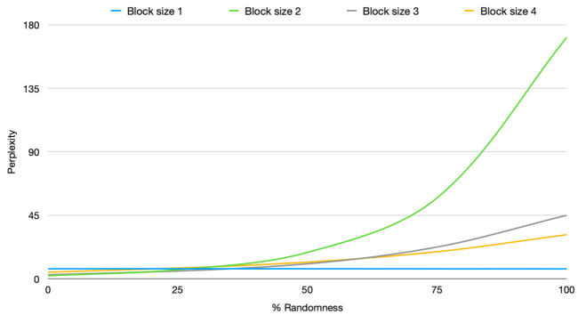
Figure 8: Perplexity vs. Randomness for varying block sizes. The degree of dependence between the labels is highest for block size = 2, where each label depends the preceding label. In such cases, the model is most affected by shuffling the order at test time. In contrast, with block size of 1, the perplexity is nearly unaffected by the order. This result complements Lemma B.3 in showing that order will not affect seq2seq models if all the labels are independent of each other.

G.1 Major Findings

We now outline our findings from the simulation. We use the architecture of bart-base Lewis et al. (2020) (six-layers of encoder and decoder) without pre-training for all simulations. All the simulations were repeated using three different random seeds, and we report the averages.

Finding 1: seq2seq models are sensitive to order, but only if the labels are conditionally dependent on each other.

We train with the prefix ${\bm{y}}_{p}$ listed in the lexicographic order. At test time, the order of is randomized from 0% (same order as training) to 100 (appendixly shuffled). As can be seen from Figure 8 the perplexity gradually increases with the degree of randomness. Further, note that perplexity is an artifact of the model and is independent of the sampling strategy used, showing that order affects learning.

Finding 2: Training with random orders makes the model less sensitive to order

As Figure 9 shows, augmenting with random order makes the model less sensitive to order. Further, augmenting with random order keeps helping as the perplexity gradually falls, and the drop shows no signs of flattening.

Finding 3: Effects of position embeddings can be overcome by augmenting with a sufficient number of random samples

Figure 9 shows that while disabling position embedding helps the baseline, similar effects are soon achieved by increasing the random order. This shows that disabling position embeddings can indeed alleviate some concerns about the order. This is crucial for pre-trained models, for which position embeddings cannot be ignored.

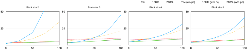
Figure 9: Augmenting dataset with multiple orders help across block sizes. Augmentations also overcome any benefit that is obtained by using position embeddings.

Finding 4: setaug leads to higher set overlap

We next consider blocks of order 2 where the prefix symbol ${\textnormal{y}}_{p}$ is selected randomly as before, but the suffix is set to a special character ${\textnormal{y}}_{p}^{\prime}$ with 50% probability. As the special symbol ${\textnormal{y}}_{p}^{\prime}$ only occurs with ${\textnormal{y}}_{p}$, there is a high pmi between each $({\textnormal{y}}_{p},{\textnormal{y}}_{p}^{\prime})$ pair as $p({\textnormal{y}}_{p}\mid{\textnormal{y}}_{p}^{\prime})=1$. Different from finding 1, the output symbols are now shuffled to mimic a realistic setup. We gradually augment the training data with random and topological orders and evaluate the learning and the final set overlap using training perplexity and Jaccard score, respectively. The results are shown in Figure 10. Similar trends hold for larger block sizes, and the results are included in the Appendix in the interest of space.

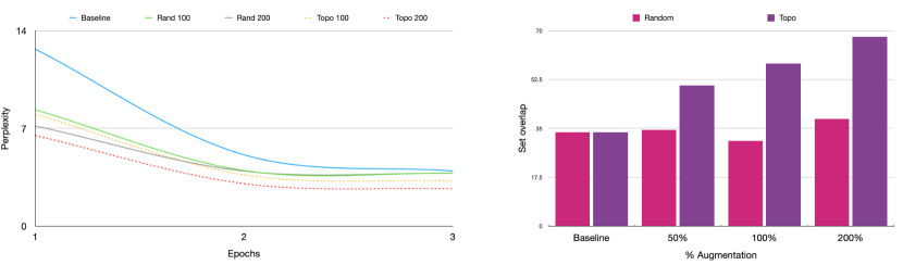
Figure 10: Effect of setaug on perplexity and set overlap. Left: Augmentations done setaug helps the model converge faster and to a lower perplexity. Right: Using setaug, the overlap between training and test set increases consistently, while consistently outperforming random.

Finding 5: setaug helps across all sampling types

We see from Table 14 that our approach is not sensitive to the sampling type used. Across five different sampling types, augmenting with topological orders yields significant gains.

Finding 6: seq2seq models can learn cardinality and use it for better decoding

We created sample data from  Figure 7 where the length of the output is determined by sum of the inputs $X$. We experimented with and without including cardinality as the first element. We found that training with cardinality increases step overlap by over 13%, from 40.54 to 46.13. Further, the version with cardinality accurately generated sets which had the same length as the target 70.64% of the times, as opposed to 27.45% for the version without cardinality.

	Beam	Random	Greedy	Top-k	Nucleus
random	$0.39\pm 0.05$	$0.39\pm 0.02$	$0.35\pm 0.05$	$0.39\pm 0.02$	$0.39\pm 0.02$
setaug	$0.67\pm 0.05$	$0.67\pm 0.05$	$0.71\pm 0.04$	$0.67\pm 0.05$	$0.68\pm 0.05$

Table 14: Set overlap for different sampling types with 200% augmentations. The gains are consistent across sampling types. Similar trends were observed for 100% augmentation and without positional embeddings. Top-k sampling was introduced by (Fan et al., 2018), and Nucleus sampling by (Holtzman et al., 2020).

Appendix H Fixing the proposal distribution in the vae formulation

$$\log p_{\theta}({\mathbb{Y}}\mid{\bm{x}}) =\log\sum_{\pi_{\bm{z}}\in\Pi}p_{\theta}(\pi_{z}({\mathbb{Y}})\mid{\bm{x}})$$

$$=\log\sum_{\pi_{\bm{z}}\in\Pi}\frac{q_{\phi}(\pi_{\bm{z}})}{q_{\phi}(\pi_{\bm{z}})}p_{\theta}(\pi_{z}({\mathbb{Y}})\mid{\bm{x}})$$

$$=\log\mathbb{E}_{q_{\phi}(\pi_{\bm{z}})}\left[\frac{p_{\theta}(\pi_{z}({\mathbb{Y}})\mid{\bm{x}})}{q_{\phi}(\pi_{\bm{z}})}\right]$$

$$\geq\mathbb{E}_{q_{\phi}(\pi_{\bm{z}})}\left[\log p_{\theta}({\mathbb{Y}},\pi_{\bm{z}}\mid{\bm{x}})\right]-\mathbb{E}_{q_{\phi}(\pi_{\bm{z}})}\left[\log q_{\phi}(\pi_{\bm{z}})\right]$$

$$\log p_{\theta}({\mathbb{Y}}\mid{\bm{x}}) =\log\sum_{\pi_{\bm{z}}\in\Pi}p_{\theta}(\pi_{z}({\mathbb{Y}})\mid{\bm{x}})$$

$$\geq\underbrace{\mathbb{E}_{q_{\phi}(\pi_{\bm{z}})}\left[\log\frac{p_{\theta}(\pi_{\bm{z}}({\mathbb{Y}})\mid{\bm{x}})}{q_{\phi}(\pi_{\bm{z}})}\right]}_{\textsc{elbo}}=\mathcal{L}(\theta,\phi)$$

Where equation LABEL:eqn:elbo is the evidence lower bound (elbo). The success of this formulation depends on the quality of the proposal distribution $q$ from which the orders are drawn. When $q$ is fixed (e.g., to uniform distribution over the orders), learning only happens for $\theta$. This can be clearly seen from splitting Equation LABEL:eqn:elbo into terms that involve just $\theta$ and $\phi$:

$$\nabla_{\phi}\mathcal{L}(\theta,\phi) =0$$

$$\nabla_{\theta}\mathcal{L}(\theta,\phi) =\nabla_{\theta}\mathbb{E}_{q_{\phi}(\pi_{\bm{z}})}\left[\log p_{\theta}({\mathbb{Y}},\pi_{\bm{z}}\mid{\bm{x}})\right]$$

Appendix I Example Appendix

This is an appendix.

References

- Brown et al. (2020) Tom B. Brown, Benjamin Mann, Nick Ryder, Melanie Subbiah, Jared Kaplan, Prafulla Dhariwal, Arvind Neelakantan, Pranav Shyam, Girish Sastry, Amanda Askell, Sandhini Agarwal, Ariel Herbert-Voss, Gretchen Krueger, Tom Henighan, Rewon Child, Aditya Ramesh, Daniel M. Ziegler, Jeffrey Wu, Clemens Winter, Christopher Hesse, Mark Chen, Eric Sigler, Mateusz Litwin, Scott Gray, Benjamin Chess, Jack Clark, Christopher Berner, Sam McCandlish, Alec Radford, Ilya Sutskever, and Dario Amodei. 2020. Language models are few-shot learners. In Advances in Neural Information Processing Systems 33: Annual Conference on Neural Information Processing Systems 2020, NeurIPS 2020, December 6-12, 2020, virtual.
- Burda et al. (2016) Yuri Burda, Roger B. Grosse, and Ruslan Salakhutdinov. 2016. Importance weighted autoencoders. In 4th International Conference on Learning Representations, ICLR 2016, San Juan, Puerto Rico, May 2-4, 2016, Conference Track Proceedings.
- Chen et al. (2021) Xiaohui Chen, Xu Han, Jiajing Hu, Francisco JR Ruiz, and Liping Liu. 2021. Order matters: Probabilistic modeling of node sequence for graph generation. arXiv preprint arXiv:2106.06189.
- Choi et al. (2018) Eunsol Choi, Omer Levy, Yejin Choi, and Luke Zettlemoyer. 2018. Ultra-fine entity typing. In Proceedings of the 56th Annual Meeting of the Association for Computational Linguistics (Volume 1: Long Papers), pages 87–96, Melbourne, Australia. Association for Computational Linguistics.
- Dai et al. (2021) Hongliang Dai, Yangqiu Song, and Haixun Wang. 2021. Ultra-fine entity typing with weak supervision from a masked language model. In Proceedings of the 59th Annual Meeting of the Association for Computational Linguistics and the 11th International Joint Conference on Natural Language Processing (Volume 1: Long Papers), pages 1790–1799, Online. Association for Computational Linguistics.
- Demszky et al. (2020) Dorottya Demszky, Dana Movshovitz-Attias, Jeongwoo Ko, Alan Cowen, Gaurav Nemade, and Sujith Ravi. 2020. GoEmotions: A dataset of fine-grained emotions. In Proceedings of the 58th Annual Meeting of the Association for Computational Linguistics, pages 4040–4054, Online. Association for Computational Linguistics.
- Domke and Sheldon (2018) Justin Domke and Daniel R. Sheldon. 2018. Importance weighting and variational inference. In Advances in Neural Information Processing Systems 31: Annual Conference on Neural Information Processing Systems 2018, NeurIPS 2018, December 3-8, 2018, Montréal, Canada, pages 4475–4484.
- Dyer et al. (2016) Chris Dyer, Adhiguna Kuncoro, Miguel Ballesteros, and Noah A. Smith. 2016. Recurrent neural network grammars. In Proceedings of the 2016 Conference of the North American Chapter of the Association for Computational Linguistics: Human Language Technologies, pages 199–209, San Diego, California. Association for Computational Linguistics.
- Fan et al. (2018) Angela Fan, Mike Lewis, and Yann Dauphin. 2018. Hierarchical neural story generation. In Proceedings of the 56th Annual Meeting of the Association for Computational Linguistics (Volume 1: Long Papers), pages 889–898, Melbourne, Australia. Association for Computational Linguistics.
- Fu et al. (2021) Zihao Fu, Wai Lam, Anthony Man-Cho So, and Bei Shi. 2021. A theoretical analysis of the repetition problem in text generation. In Proceedings of the AAAI Conference on Artificial Intelligence, volume 35, pages 12848–12856.
- Hagberg et al. (2008) Aric Hagberg, Pieter Swart, and Daniel S Chult. 2008. Exploring network structure, dynamics, and function using networkx. Technical report, Los Alamos National Lab.(LANL), Los Alamos, NM (United States).
- Holtzman et al. (2020) Ari Holtzman, Jan Buys, Li Du, Maxwell Forbes, and Yejin Choi. 2020. The curious case of neural text degeneration. In 8th International Conference on Learning Representations, ICLR 2020, Addis Ababa, Ethiopia, April 26-30, 2020. OpenReview.net.
- Huang et al. (2020) Qian Huang, Horace He, Abhay Singh, Yan Zhang, Ser-Nam Lim, and Austin R. Benson. 2020. Better set representations for relational reasoning. In Advances in Neural Information Processing Systems 33: Annual Conference on Neural Information Processing Systems 2020, NeurIPS 2020, December 6-12, 2020, virtual.
- Hwang et al. (2021) Jena D Hwang, Chandra Bhagavatula, Ronan Le Bras, Jeff Da, Keisuke Sakaguchi, Antoine Bosselut, and Yejin Choi. 2021. (comet-) atomic 2020: On symbolic and neural commonsense knowledge graphs. In Proceedings of the AAAI Conference on Artificial Intelligence, volume 35, pages 6384–6392.
- Jin et al. (2018) Wengong Jin, Regina Barzilay, and Tommi S. Jaakkola. 2018. Junction tree variational autoencoder for molecular graph generation. In Proceedings of the 35th International Conference on Machine Learning, ICML 2018, Stockholmsmässan, Stockholm, Sweden, July 10-15, 2018, volume 80 of Proceedings of Machine Learning Research, pages 2328–2337. PMLR.
- Johnson et al. (2000) Richard A Johnson, Irwin Miller, and John E Freund. 2000. Probability and statistics for engineers, volume 2000. Pearson Education London.
- Ju et al. (2020) Xincheng Ju, Dong Zhang, Junhui Li, and Guodong Zhou. 2020. Transformer-based label set generation for multi-modal multi-label emotion detection. In MM ’20: The 28th ACM International Conference on Multimedia, Virtual Event / Seattle, WA, USA, October 12-16, 2020, pages 512–520.
- Khandelwal et al. (2018) Urvashi Khandelwal, He He, Peng Qi, and Dan Jurafsky. 2018. Sharp nearby, fuzzy far away: How neural language models use context. In Proceedings of the 56th Annual Meeting of the Association for Computational Linguistics (Volume 1: Long Papers), pages 284–294, Melbourne, Australia. Association for Computational Linguistics.
- Kim et al. (2021) Jinwoo Kim, Jaehoon Yoo, Juho Lee, and Seunghoon Hong. 2021. Setvae: Learning hierarchical composition for generative modeling of set-structured data. In Proceedings of the IEEE/CVF Conference on Computer Vision and Pattern Recognition, pages 15059–15068.
- Kosiorek et al. (2020) Adam R Kosiorek, Hyunjik Kim, and Danilo J Rezende. 2020. Conditional set generation with transformers. arXiv preprint arXiv:2006.16841.
- Lee et al. (2019) Juho Lee, Yoonho Lee, Jungtaek Kim, Adam R. Kosiorek, Seungjin Choi, and Yee Whye Teh. 2019. Set transformer: A framework for attention-based permutation-invariant neural networks. In Proceedings of the 36th International Conference on Machine Learning, ICML 2019, 9-15 June 2019, Long Beach, California, USA, volume 97 of Proceedings of Machine Learning Research, pages 3744–3753. PMLR.
- Lewis (1997) David Lewis. 1997. Reuters-21578 text categorization test collection, distribution 1.0. http://www. research/. att. com.
- Lewis et al. (2020) Mike Lewis, Yinhan Liu, Naman Goyal, Marjan Ghazvininejad, Abdelrahman Mohamed, Omer Levy, Veselin Stoyanov, and Luke Zettlemoyer. 2020. BART: Denoising sequence-to-sequence pre-training for natural language generation, translation, and comprehension. In Proceedings of the 58th Annual Meeting of the Association for Computational Linguistics, pages 7871–7880, Online. Association for Computational Linguistics.
- Liu et al. (2021) Pengfei Liu, Weizhe Yuan, Jinlan Fu, Zhengbao Jiang, Hiroaki Hayashi, and Graham Neubig. 2021. Pre-train, prompt, and predict: A systematic survey of prompting methods in natural language processing. ArXiv.
- Meng et al. (2019) Rui Meng, Xingdi Yuan, Tong Wang, Peter Brusilovsky, Adam Trischler, and Daqing He. 2019. Does order matter? an empirical study on generating multiple keyphrases as a sequence. arXiv preprint arXiv:1909.03590.
- Meng et al. (2017) Rui Meng, Sanqiang Zhao, Shuguang Han, Daqing He, Peter Brusilovsky, and Yu Chi. 2017. Deep keyphrase generation. In Proceedings of the 55th Annual Meeting of the Association for Computational Linguistics (Volume 1: Long Papers), pages 582–592, Vancouver, Canada. Association for Computational Linguistics.
- Murphy et al. (2019) Ryan L. Murphy, Balasubramaniam Srinivasan, Vinayak A. Rao, and Bruno Ribeiro. 2019. Janossy pooling: Learning deep permutation-invariant functions for variable-size inputs. In 7th International Conference on Learning Representations, ICLR 2019, New Orleans, LA, USA, May 6-9, 2019. OpenReview.net.
- Nag Chowdhury et al. (2016) Sreyasi Nag Chowdhury, Niket Tandon, and Gerhard Weikum. 2016. Know2Look: Commonsense knowledge for visual search. In Proceedings of the 5th Workshop on Automated Knowledge Base Construction, pages 57–62, San Diego, CA. Association for Computational Linguistics.
- Nandwani et al. (2020) Yatin Nandwani, Deepanshu Jindal, Parag Singla, et al. 2020. Neural learning of one-of-many solutions for combinatorial problems in structured output spaces. arXiv preprint arXiv:2008.11990.
- OpenAI (2021) OpenAI. 2021. Openai completion engine (davinci) api.
- Qin et al. (2019) Kechen Qin, Cheng Li, Virgil Pavlu, and Javed Aslam. 2019. Adapting RNN sequence prediction model to multi-label set prediction. In Proceedings of the 2019 Conference of the North American Chapter of the Association for Computational Linguistics: Human Language Technologies, Volume 1 (Long and Short Papers), pages 3181–3190, Minneapolis, Minnesota. Association for Computational Linguistics.
- Raffel et al. (2020) Colin Raffel, Noam Shazeer, Adam Roberts, Katherine Lee, Sharan Narang, Michael Matena, Yanqi Zhou, Wei Li, and Peter J Liu. 2020. Exploring the limits of transfer learning with a unified text-to-text transformer. Journal of Machine Learning Research, 21:1–67.
- Rezatofighi et al. (2018) S Hamid Rezatofighi, Roman Kaskman, Farbod T Motlagh, Qinfeng Shi, Daniel Cremers, Laura Leal-Taixé, and Ian Reid. 2018. Deep perm-set net: Learn to predict sets with unknown permutation and cardinality using deep neural networks. arXiv preprint arXiv:1805.00613.
- Santoro et al. (2017) Adam Santoro, David Raposo, David G. T. Barrett, Mateusz Malinowski, Razvan Pascanu, Peter W. Battaglia, and Tim Lillicrap. 2017. A simple neural network module for relational reasoning. In Advances in Neural Information Processing Systems 30: Annual Conference on Neural Information Processing Systems 2017, December 4-9, 2017, Long Beach, CA, USA, pages 4967–4976.
- Vaswani et al. (2017) Ashish Vaswani, Noam Shazeer, Niki Parmar, Jakob Uszkoreit, Llion Jones, Aidan N. Gomez, Lukasz Kaiser, and Illia Polosukhin. 2017. Attention is all you need. In Advances in Neural Information Processing Systems 30: Annual Conference on Neural Information Processing Systems 2017, December 4-9, 2017, Long Beach, CA, USA, pages 5998–6008.
- Vinyals et al. (2016) Oriol Vinyals, Samy Bengio, and Manjunath Kudlur. 2016. Order matters: Sequence to sequence for sets. In 4th International Conference on Learning Representations, ICLR 2016, San Juan, Puerto Rico, May 2-4, 2016, Conference Track Proceedings.
- Wang et al. (2021) Ruize Wang, Duyu Tang, Nan Duan, Zhongyu Wei, Xuanjing Huang, Jianshu Ji, Guihong Cao, Daxin Jiang, and Ming Zhou. 2021. K-Adapter: Infusing Knowledge into Pre-Trained Models with Adapters. In Findings of the Association for Computational Linguistics: ACL-IJCNLP 2021, pages 1405–1418, Online. Association for Computational Linguistics.
- Welleck et al. (2020) Sean Welleck, Ilia Kulikov, Stephen Roller, Emily Dinan, Kyunghyun Cho, and Jason Weston. 2020. Neural text generation with unlikelihood training. In 8th International Conference on Learning Representations, ICLR 2020, Addis Ababa, Ethiopia, April 26-30, 2020. OpenReview.net.
- Wettler and Rapp (1993) Manfred Wettler and Reinhard Rapp. 1993. Computation of word associations based on co-occurrences of words in large corpora. In Very Large Corpora: Academic and Industrial Perspectives.
- Wolf et al. (2019) Thomas Wolf, Lysandre Debut, Victor Sanh, Julien Chaumond, Clement Delangue, Anthony Moi, Pierric Cistac, Tim Rault, Rémi Louf, Morgan Funtowicz, et al. 2019. Huggingface’s transformers: State-of-the-art natural language processing. arXiv preprint arXiv:1910.03771.
- Yang et al. (2019a) Pengcheng Yang, Fuli Luo, Shuming Ma, Junyang Lin, and Xu Sun. 2019a. A deep reinforced sequence-to-set model for multi-label classification. In Proceedings of the 57th Annual Meeting of the Association for Computational Linguistics, pages 5252–5258, Florence, Italy. Association for Computational Linguistics.
- Yang et al. (2018) Pengcheng Yang, Xu Sun, Wei Li, Shuming Ma, Wei Wu, and Houfeng Wang. 2018. SGM: Sequence generation model for multi-label classification. In Proceedings of the 27th International Conference on Computational Linguistics, pages 3915–3926, Santa Fe, New Mexico, USA. Association for Computational Linguistics.
- Yang et al. (2020) Yiben Yang, Chaitanya Malaviya, Jared Fernandez, Swabha Swayamdipta, Ronan Le Bras, Ji-Ping Wang, Chandra Bhagavatula, Yejin Choi, and Doug Downey. 2020. G-daug: Generative data augmentation for commonsense reasoning. In Proceedings of the 2020 Conference on Empirical Methods in Natural Language Processing: Findings, pages 1008–1025.
- Yang et al. (2019b) Zhilin Yang, Zihang Dai, Yiming Yang, Jaime G. Carbonell, Ruslan Salakhutdinov, and Quoc V. Le. 2019b. Xlnet: Generalized autoregressive pretraining for language understanding. In Advances in Neural Information Processing Systems 32: Annual Conference on Neural Information Processing Systems 2019, NeurIPS 2019, December 8-14, 2019, Vancouver, BC, Canada, pages 5754–5764.
- Ye et al. (2021) Jiacheng Ye, Tao Gui, Yichao Luo, Yige Xu, and Qi Zhang. 2021. One2Set: Generating diverse keyphrases as a set. In Proceedings of the 59th Annual Meeting of the Association for Computational Linguistics and the 11th International Joint Conference on Natural Language Processing (Volume 1: Long Papers), pages 4598–4608, Online. Association for Computational Linguistics.
- Yuan et al. (2020) Xingdi Yuan, Tong Wang, Rui Meng, Khushboo Thaker, Peter Brusilovsky, Daqing He, and Adam Trischler. 2020. One size does not fit all: Generating and evaluating variable number of keyphrases. In Proceedings of the 58th Annual Meeting of the Association for Computational Linguistics, pages 7961–7975, Online. Association for Computational Linguistics.
- Zaheer et al. (2017) Manzil Zaheer, Satwik Kottur, Siamak Ravanbakhsh, Barnabás Póczos, Ruslan Salakhutdinov, and Alexander J. Smola. 2017. Deep sets. In Advances in Neural Information Processing Systems 30: Annual Conference on Neural Information Processing Systems 2017, December 4-9, 2017, Long Beach, CA, USA, pages 3391–3401.
- Zhang et al. (2019a) Yan Zhang, Jonathon S. Hare, and Adam Prügel-Bennett. 2019a. Deep set prediction networks. In Advances in Neural Information Processing Systems 32: Annual Conference on Neural Information Processing Systems 2019, NeurIPS 2019, December 8-14, 2019, Vancouver, BC, Canada, pages 3207–3217.
- Zhang et al. (2019b) Zhengyan Zhang, Xu Han, Zhiyuan Liu, Xin Jiang, Maosong Sun, and Qun Liu. 2019b. ERNIE: Enhanced language representation with informative entities. In Proceedings of the 57th Annual Meeting of the Association for Computational Linguistics, pages 1441–1451, Florence, Italy. Association for Computational Linguistics.