Constraints on the two-dimensional pseudo-spin 1/2 Mott insulator description of Sr₂IrO₄

Abstract

Sr₂IrO₄ has often been described via a simple, one-band pseudo-spin 1/2 model, subject to electron-electron interactions, on a square lattice, fostering analogies with cuprate superconductors, believed to be well described by a similar model. In this work we argue – based on a detailed study of the low-energy electronic structure by circularly polarized spin and angle-resolved photoemission spectroscopy combined with dynamical mean-field theory calculations – that a pseudo-spin 1/2 model fails to capture the full complexity of the system. We show instead that a realistic multi-band Hubbard Hamiltonian, accounting for the full correlated $t_{2g}$ manifold, provides a detailed description of the interplay between spin-orbital entanglement and electron-electron interactions, and yields quantitative agreement with experiments. Our analysis establishes that the $j_{3/2}$ states make up a substantial percentage of the low energy spectral weight, i.e. approximately 74% as determined from the integration of the $j$-resolved spectral function in the $0$ to $-1.64$ eV energy range. The results in our work are not only of relevance to iridium based materials, but more generally to the study of multi-orbital materials with closely spaced energy scales.

I Introduction

Sr₂IrO₄ has been studied since shortly after the discovery of the cuprate superconductors [1, 2], as the compound was believed to share some of its defining properties with the copper oxides. More specifically, Sr₂IrO₄ shares its structure with the superconducting “parent compound” La₂CuO₄, and it features a similar anti ferromagnetic ground state [2, 3, 4]. A key difference is that the cuprates are described by a single hole in the $e_{g}$ manifold, as opposed to the iridate that has a single hole in the $t_{2g}$ manifold. In the seminal work by Kim et al., it was suggested that the $t_{2g}$ orbitals entangle into a filled $j_{\mathrm{eff}}=3/2$, and a half filled $j_{\mathrm{eff}}=1/2$ manifold [5]. It was quickly realized that this scenario would bring Sr₂IrO₄ even closer to the quintessential cuprate superconductor: a (pseudo-) spin 1/2 Mott insulator on a square two-dimensional lattice. Theoretical calculations predicted a superconducting state may exist in a $j_{\mathrm{eff}}$ pseudo-spin 1/2 system when electron doped [6], with more sophisticated analyses including all $t_{2g}$ orbitals and strong spin-orbit coupling painting a similar picture [7, 8]. Promising observations were made in experiments: it was found that the excitations of the pseudospins probed by resonant inelastic x-ray scattering (RIXS) are reminiscent of a Heisenberg model [9, 10], the expected low energy behaviour for a spin 1/2 Mott insulator [11, 12]. In addition, features reminiscent of doped Mott insulators, such as a v-shaped gap and a phase separated spatial distribution, were seen in scanning tunnelling microscopy (STM) [13], and a pseudogap was detected in angle-resolved photoemission spectroscopy (ARPES) [14]. Even stronger evidence was found in surface doped samples: STM and ARPES observe a gap that reminds of those found in cuprate superconductors [15, 16]. However, these are spectroscopic observations that are constrained to the surface, and so far no signatures of bulk superconducting behaviour have been reported in the literature.

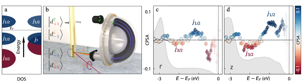
Figure 1: (a) Schematic representation of a fully decoupled pseudo-spin 1/2 model (left), and an entangled multi-orbital Mott system (right). (b) Schematic depiction of the circularly polarized spin-ARPES (CPS ARPES) experiment. Different spin-orbitally entangled states $\ket{d_{m_{\ell}}^{m_{s}}}$ can be selected by choosing a combination of circular polarization $\{\oplus,\ominus\}$ and spin-detector channel $\{\uparrow,\downarrow\}$. (c,d) The CPS ARPES intensity obtained at normal emission using 51.1 (c) and 64 (d) eV photons corresponding to the $\Gamma$ and $\mathrm{Z}$ points in the Brillouin zone respectively (colored markers), and the sum of spin and polarization dependent signals (grey shaded).

A potential factor in the explanation for the lack of superconductivity may be found in the non-trivial departure from a simple spin 1/2 scenario. We start by pointing out that the theoretical models predicting superconductivity have been derived in the strong spin-orbit coupling limit [6, 7, 8] (i.e. in the limit of a “simple” pseudo-spin 1/2 model). Although spin-orbit coupling is large in this system ($\sim 0.45$ eV [17, 18, 10]), it is still modest compared to the overall bandwidth ($\sim 2$ eV) of the $t_{2g}$ bands [19, 20, 21]. A complete splitting into $j_{3/2}$ and $j_{1/2}$ multiplets is therefore likely not realized, and there has been some sporadic evidence that supports this idea. It was pointed out that toward the Brillouin zone boundaries, the pristine $t_{2g}$ character dominates the spin-orbital entanglement, and not much mixing occurs [21]. Neutron scattering shows that the local moments are far from the idealized $j_{1/2}$ picture, and in reality the eigenstates bear more resemblance to a $d_{xy}$ orbital [23]. Taken altogether, these arguments suggest that a pseudo-spin 1/2 model may not be a sufficient description of the system, and raise questions about the true nature of the Sr₂IrO₄ ground state.

In this paper, we use a technique that can directly attend to the question of whether a pseudo-spin 1/2 model is indeed a valid description for Sr₂IrO₄. In order to do this, we measure the spin-orbital entanglement of the valence band states, i.e. the expectation value $\expectationvalue{\mathbf{L}\cdot\mathbf{S}}$ for the low energy states, using circularly polarized spin-ARPES (CPS-ARPES) and observe a clear departure from the canonical $j_{1/2}$ model. We are instead able to explain our observations using dynamical mean field theory (DMFT) calculations, which accurately predict the non-trivial behavior of this multi-band, spin-orbit coupled Mott system, without imposing a predefined hierarchy onto the magnitudes of these effects. Our conclusion is that a spin 1/2 model is insufficient to capture all intricacies of the low energy electronic structure of this material, but more importantly that we gain a strong understanding of Sr₂IrO₄ by comparing our experiments to an adequately powerful theoretical description.

To make substantiated arguments about the sufficiency of the $j_{1/2}$ model, the quantum number $j$ should be measured for the low energy manifold, giving a distinct character for the $j_{1/2}$ and $j_{3/2}$ states. If the system can be described as a pseudo-spin 1/2 system, the $j_{3/2}$ states must be far enough into the valence bands so that they do not overlap with, or couple to, the $j_{1/2}$ states [Fig. 1 (a), left]. A sizeable overlap or coupling would result in bands with both $j_{1/2}$ and $j_{3/2}$ character [Fig. 1 (a), right]. However, while the quantum number $j$ is not directly accessible in ARPES measurements, the alignment of spin and orbital angular momentum $\expectationvalue{\mathbf{L}\cdot\mathbf{S}}$, which has an immediate relation to $j$, can be measured directly. For a pure $j_{1/2}$ state this quantity should be positive ($\expectationvalue{\mathbf{L}\cdot\mathbf{S}}=1$), while it would be negative for a pure $j_{3/2}$ state ($\expectationvalue{\mathbf{L}\cdot\mathbf{S}}=-\frac{1}{2}$) .

II Circularly Polarized Spin ARPES

To quantify the spin-orbital entanglement, spin-resolved measurements are performed using circularly polarized light, as schematically depicted in Fig. 1 (b). This technique has been used previously in angle-integrated photoemission [25, 26], as well as in ARPES on Sr₂RuO₄ [27] and iron pnictides [28]. The use of circularly polarized light selects a particular $m_{\ell}$ value $\{-1,+1\}$, through the photoemission dipole matrix element, while the spin-detector selects between states with $m_{s}=\{\uparrow,\downarrow\}$. By combining these two filters, and measuring the four individual components, it is possible to obtain the spin-orbital entanglement. In particular, it can be shown that at normal emission, the $z$ component of $\expectationvalue{\mathbf{L}\cdot\mathbf{S}}$, i.e. $\expectationvalue{L_{z}S_{z}}$, can be recovered.

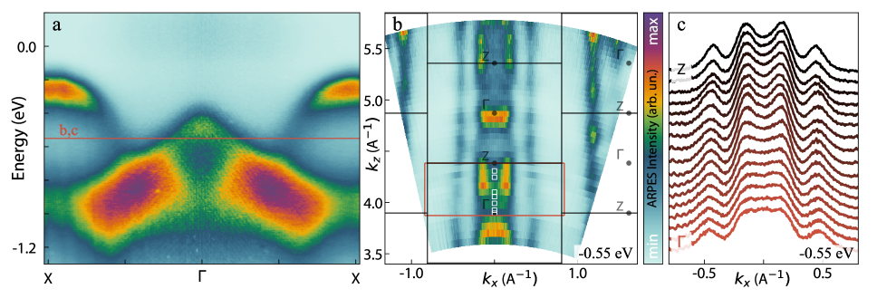
Figure 2: Overview of photon energy dependent results in Sr₂IrO₄. (a) Spectrum at $h\nu=100$ eV ($k_{z}=5.29$ Å^-1). The red line indicates the energy ($E=-0.55$ eV) at which the plots presented in panels (b) and (c) have been generated. (b) Constant energy map at $E=-0.55$ eV, using a sum of $\sigma$ and $\pi$-polarized light. The white boxes indicate the positions of later presented CPS ARPES data. (c) A series of MDCs measured with photon energies ranging from $h\nu=51$ eV ($k_{z}=3.89$ Å^-1) to $h\nu=84$ eV ($k_{z}=4.87$ Å^-1), with $\sigma$-polarization at $E=-0.55$ eV; the ($k_{x},k_{z}$) area encompassed is indicated by a red box in (b).

To derive this property, we start by considering the photoemission dipole matrix element, arising from Fermi’s golden rule (for a thorough review, the reader is referred to [29])

$$M_{i,f}^{\varepsilon,\sigma,k}=\matrixelement{\psi_{f}^{k}}{\mathbf{r}\cdot\bm{\varepsilon}}{\phi_{i}}=\\ \sum_{\begin{subarray}{c}\ell_{i},\ell_{f},m_{i}\\ m_{\varepsilon},m_{f}\end{subarray}}c_{l_{i}}^{m_{i}}B_{n_{i},\ell_{i},\ell_{f}}\matrixelement{Y^{m_{i}}_{\ell_{i}}}{Y^{m_{\varepsilon}}_{1}}{Y^{m_{f}}_{\ell_{f}}}Y^{m_{f}}_{\ell_{f}}\left(\theta_{\mathbf{k}},\phi_{\mathbf{k}}\right).$$ (1)

with $\ket{\psi_{f}^{k}}$ and $\ket{\phi_{i}}$ the final and initial states respectively, $\bm{\varepsilon}$ the polarization vector, $c_{l_{i}}^{m_{i}}$ the initial state coefficient in the basis of spherical harmonics, and $B_{n_{i},\ell_{i},\ell_{f}}$ a radial integral:

$$B_{n_{i},\ell_{i},\ell_{f}}=\int drr^{3}R_{n_{i},\ell_{i}}(r)j_{\ell_{f}}(r),$$ (2)

where $R_{n_{i},\ell_{i}}(r)$ is the radial part of the basis functions and $j_{\ell_{f}}(r)$ are the spherical Bessel functions. Using circularly polarized light with positive helicity gives $\bm{\varepsilon}^{\oplus}\cdot\mathbf{r}=\varepsilon_{0}\left(x+iy\right)=\varepsilon_{0}Y^{1}_{1}$. The matrix element then becomes:

$$M_{i,f}^{k}=\matrixelement{\psi_{f}^{k}}{\mathbf{r}\cdot\bm{\varepsilon}}{\phi_{i}}=\\ \varepsilon_{0}\sum_{\begin{subarray}{c}\ell_{f}\\ m_{f},m_{i}\end{subarray}}c_{l_{i}}^{m_{i}}B_{n_{i},\ell_{i},\ell_{f}}\matrixelement{Y^{m_{f}}_{\ell_{f}}}{Y^{1}_{1}}{Y^{m_{i}}_{\ell_{i}}}Y^{m_{f}}_{l_{f}}\left(\theta_{k},\phi_{k}\right),$$ (3)

At the $\Gamma$ point, we can simplify this equation by using the fact that the spherical harmonic $Y^{m_{f}}_{l_{f}}\left(\theta_{k},\phi_{k}\right)$ has nodes for all $m_{f}$ except $m_{f}=0$, where its value is 1. With the spherical harmonic arising from the polarization vector set to $Y^{1}_{1}$, we only emit from a single initial state spherical harmonic. We can therefore simplify the expression in Eq. 3 to:

$$M_{i,f}^{k\sigma}=\varepsilon_{0}\sum_{\ell_{f}}c^{m_{i}=-1,\sigma}_{\ell_{i}}B_{n_{i},\ell_{i},\ell_{f}}\matrixelement{Y^{0}_{\ell_{f}}}{Y^{1}_{1}}{Y^{-1}_{\ell_{i}}}.$$ (4)

Noting that the product of spherical harmonics does not depend on $m_{i}$, we can take the sum over $\ell_{f}$ up into a constant prefactor. We denote $a_{\ell_{i},\ell_{f}}=\matrixelement{Y^{0}_{\ell_{f}}}{Y^{1}_{1}}{Y^{-1}_{\ell_{i}}}$. To get the photoemission intensity, we take the squared norm:

$$I^{\oplus\sigma}=\varepsilon_{0}^{2}\left(\sum_{\ell_{f}}B_{n_{i},\ell_{i},\ell_{f}}a_{\ell_{i},\ell_{f}}\right)^{2}\absolutevalue{c^{m_{i}=-1,\sigma}_{\ell_{i}}}^{2}\\ =A\absolutevalue{c^{-1,\sigma}_{\ell_{i}}}^{2}.$$ (5)

It follows trivially that we can measure the other components using $\sigma=\uparrow,\downarrow$ and $\varepsilon=\oplus,\ominus$ to construct:

$$I^{\ominus\uparrow}-I^{\oplus\uparrow}-I^{\ominus\downarrow}+I^{\oplus\downarrow}\\ =A\left(\absolutevalue{c^{1,\uparrow}}^{2}-\absolutevalue{c^{-1,\uparrow}}^{2}-\absolutevalue{c^{1,\downarrow}}^{2}+\absolutevalue{c^{-1,\downarrow}}^{2}\right)$$ (6)

Noting that in the basis of $\ket{m_{l}=1,\uparrow}$, $\ket{-1,\uparrow}$, $\ket{1,\downarrow}$, $\ket{-1,\downarrow}$, we have:

$$L_{z}S_{z}=\frac{\hbar^{2}}{2}\begin{pmatrix}1&0&0&0\\ 0&-1&0&0\\ 0&0&-1&0\\ 0&0&0&1\\ \end{pmatrix},$$ (7)

we get for $\expectationvalue{L_{z}S_{z}}$:

$$\expectationvalue{L_{z}S_{z}}=\frac{\hbar^{2}}{2}\left(\absolutevalue{c^{1,\uparrow}}^{2}-\absolutevalue{c^{-1,\uparrow}}^{2}-\absolutevalue{c^{1,\downarrow}}^{2}+\absolutevalue{c^{-1,\downarrow}}^{2}\right),$$ (8)

which is precisely the expression found in Eq. 6, aside from the prefactor. Note that the expression derived above is independent (up to the prefactor $A$) of the values for $B_{n_{i},\ell_{i},\ell_{f}}$. Since there is only a single term of $m_{l_{i}}$ for each configuration, there are no interference terms and the sum in Eq. 5 can be evaluated separately. This formulation of $\expectationvalue{L_{z}S_{z}}$ in terms of $I^{\varepsilon,\sigma}$ is unfortunately only valid if all factors $B_{n_{i},\ell_{i},\ell_{f}}$ are the identical for both polarizations $\varepsilon^{\oplus}$ and $\varepsilon^{\ominus}$, which may not be the case in a system where there is circular dichroism. Moreover, if the sensitivity of the spin-detectors is not equal for up and down channels, the description also breaks down. By denoting the sensitivity of the detector of each spin detector as $\eta^{\sigma}$, and the factor related to the circular dichroism as $\alpha^{\varepsilon}$, we can write the measured photoemission signal as:

$$\tilde{I}^{\varepsilon\sigma}=\alpha^{\varepsilon}\eta^{\sigma}I^{\varepsilon,\sigma}=\alpha^{\varepsilon}\eta^{\sigma}A\absolutevalue{c^{m_{i},\sigma}_{\ell_{i}}}^{2},$$ (9)

where $m_{i}=-1$ for $\varepsilon^{\oplus}$ and 1 for $\varepsilon^{\ominus}$. Substituting the $\tilde{I}$ into Eq. 6, the expectation value $\expectationvalue{L_{z}S_{z}}$ is no longer recovered as a result of the prefactors. We can instead take advantage of the geometric mean $P$ which divides out the prefactors:

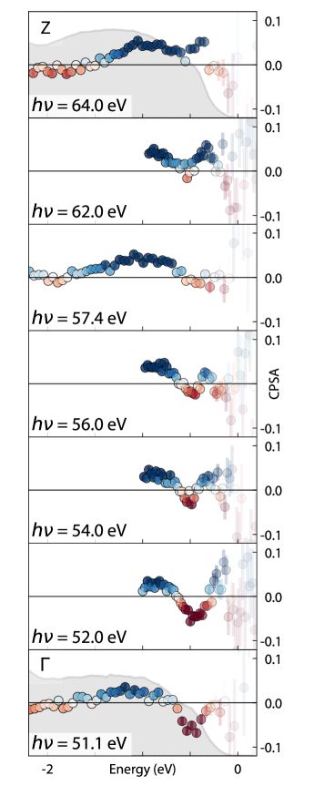
Figure 3: CPS ARPES measurements (colored markers), for photon energies ranging from 51.1 eV to 64 eV. The sum of spin and polarization dependent signals (grey shaded) corresponds to spin-integrated ARPES.

$$P=\frac{\sqrt{\tilde{I}^{\ominus\uparrow}\tilde{I}^{\oplus\downarrow}}-\sqrt{\tilde{I}^{\oplus\uparrow}\tilde{I}^{\ominus\downarrow}}}{\sqrt{\tilde{I}^{\ominus\uparrow}\tilde{I}^{\oplus\downarrow}}+\sqrt{\tilde{I}^{\oplus\uparrow}\tilde{I}^{\ominus\downarrow}}}\\ =\frac{\sqrt{\absolutevalue{c^{1,\uparrow}}^{2}\absolutevalue{c^{-1,\downarrow}}^{2}}-\sqrt{\absolutevalue{c^{-1,\uparrow}}^{2}\absolutevalue{c^{1,\downarrow}}^{2}}}{\sqrt{\absolutevalue{c^{1,\uparrow}}^{2}\absolutevalue{c^{-1,\downarrow}}^{2}}+\sqrt{\absolutevalue{c^{-1,\uparrow}}^{2}\absolutevalue{c^{1,\downarrow}}^{2}}}.$$ (10)

In the case of Kramers degeneracy, we should have $\absolutevalue{c^{m,\sigma}}^{2}=\absolutevalue{c^{-m,\bar{\sigma}}}^{2}$, and using the fact that the states are normalized ($\sum\absolutevalue{c^{m,\sigma}}^{2}=1$) we obtain:

$$P=\frac{\absolutevalue{c^{1,\uparrow}}^{2}-\absolutevalue{c^{1,\downarrow}}^{2}}{\absolutevalue{c^{1,\uparrow}}^{2}+\absolutevalue{c^{1,\downarrow}}^{2}}\\ =\absolutevalue{c^{1,\uparrow}}^{2}-\absolutevalue{c^{1,\downarrow}}^{2}-\absolutevalue{c^{-1,\uparrow}}^{2}+\absolutevalue{c^{-1,\downarrow}}^{2}=\frac{2}{\hbar^{2}}\expectationvalue{L_{z}S_{z}}.$$ (11)

Using the geometric mean, we can thus extract the expectation value for $\expectationvalue{L_{z}S_{z}}$ without the need to know the exact detector sensitivities or circular dichroism effects.

III Experimental Results

Spin-resolved measurements were performed at the VESPA endstation [30] at the Elettra Sincrotrone Trieste, using VLEED spin detectors. We present the result of applying CPS-ARPES to Sr₂IrO₄ in Fig. 1 (c,d), which display the observed CPS ARPES intensity (colored markers) at normal emission using 51.1 eV ($\Gamma$) and 64 eV ($Z$) photons respectively. The grey shaded curves represent the sums of all signals (corresponding to spin-integrated ARPES). Comparing panels (b) and (c,d) we can readily identify various features: negative ($-2$ eV) and positive ($-1$ eV) regions, belonging respectively to states with $j_{3/2}$ and $j_{1/2}$ character. Although the data from the $Z$ point in the Brillouin zone [Fig. 1 (d)] are in line with a simple pseudo-spin 1/2 picture, the strong negative signal around $E=-0.5$ eV at the $\Gamma$ point [Fig. 1 (c)] appears to be inconsistent. In the remainder of the paper we will show that this indeed constitutes a violation of the pseudo-spin 1/2 picture.

First we will provide a more detailed analysis along different crystal momenta, to capture a more complete picture of the spin-orbital entanglement. We note that while it is possible to measure CPS ARPES along the in-plane momentum ($k_{x},k_{y}$), data taken this way are much more challenging to interpret. We have nevertheless measured in-plane CPS ARPES, for which the data and corresponding analysis can be seen in full in the appendix. Here instead we focus our attention on $k_{z}$, also in light of the puzzling results in Fig. 1. In ARPES measurements, the perpendicular momentum ($k_{z}$) is accessible through changing the incident photon energy. Although Sr₂IrO₄ is quasi-two-dimensional, the extended Ir $5d$ orbitals have the potential to magnify the out of plane hopping. The $k_{z}$ dispersion in Sr₂IrO₄ and the related bilayer Sr₂Ir₂O₇ compound has been studied previously [31], and a modest energy dispersion was observed at the $X$ point. However, no data has been presented at normal emission, which is where our study is concerned.

To provide some context for the forthcoming CPS ARPES data, we first consider spin-integrated photon energy dependent ARPES data. Photon energy dependent spin-integrated ARPES measurements presented here were taken at the MERLIN beamline of the Advanced Light Source. Data were acquired between 50 and 120 eV. The data are corrected using an inner potential [32] $V_{0}=11$ eV, in good agreement with earlier published results [31]. We plot a valence band mapping of Sr₂IrO₄ along the $\Gamma-\mathrm{X}$ in Fig. 2(a). A constant energy map at $E=-0.55$ eV in the $k_{z}-k_{x}$ plane is displayed in Fig. 2(b), for a sum of $\pi$- and $\sigma$-polarization. The modulated intensity changes, especially those periodic in $k_{z}$, are a clear sign of interlayer coupling, and of an underlying $k_{z}$ dispersion. A closer inspection reveals pinching of the cylindrical state around $\Gamma$, which becomes particularly clear when considering momentum distribution curves (MDCs) between $\Gamma$ and $Z$ [Fig. 2(c)]. Although we find clear evidence of $k_{z}$ dispersion in the exposition of MDCs, the broad nature of the bands makes observing a simple periodic oscillation in the corresponding energy distribution curves (EDCs) more challenging. We also note that the energy scale appears significantly smaller than the in-plane bandwidth ($\sim$ 1-2 eV), or even the spin-orbit coupling parameter ($\sim 0.45$ eV); however, as pointed out in previous work on Sr₂RuO₄ [27], states close to degeneracies can undergo significant changes as a result of spin-orbit coupling effects, which in turn can lead to a remarkable $k_{z}$ dependence of the character of the eigenstates even though a sizable energy dispersion is notably absent.

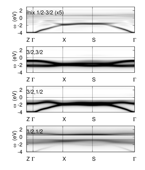
Figure 4: Diagonal and off-diagonal components of the spectral function in the $j$ basis.

We now return to CPS ARPES experiments, focusing purely on normal emission measurements, and changing $k_{z}$ only through adjusting the photon energy of the incident beam. We would like to reiterate that in this case the CPS ARPES measurement is directly proportional to the expectation value of $\expectationvalue{L_{z}S_{z}}$, and photoemission matrix element effects cancel out completely. Photon energy dependent CPS ARPES results are presented in Fig. 3 as colored markers. A grey background indicates the sum of all four individual spin- and light-polarization dependent signals, which corresponds to spin-integrated photoemission. The progression of the CPS ARPES signal is evident, and provides context and additional proof for the puzzling result first presented in Fig. 1. Although the positive and negative signal around $E=-1$ and $-2$ eV is present in all the spectra, the data at low binding energies paint a contrasting picture. The peak in the spectrum at $E=-0.5$ eV that starts out negative in Fig. 3 at 51.1 eV ($\Gamma$) can be seen to change sign as the photon energy increases to 64 eV ($Z$). It should be stressed that this is an important result: the character of the spin-orbital entanglement of the lowest-energy band changes from parallel to antiparallel upon varying $k_{z}$, revealing a drastic change in the character of the lowest-energy eigenstates. Neither this sign reversal nor the negative signal observed at $\Gamma$ are reconcilable with a simple pseudo-spin model, and require us to rethink our description of the low-energy states of Sr₂IrO₄.

IV Comparison to DMFT

We now attempt to shed light on our observations by constructing and solving a model that goes beyond the pseudo-spin 1/2 framework. To this end, we turn to dynamical mean field theory (DMFT) calculations for a realistic multi-band Hubbard Hamiltonian. The method adopted can be summarized as follows. We calculate the electronic structure (including spin-orbit effects) in the local-density approximation (LDA) via the full-potential linearized augmented plane-wave method, as implemented in the WIEN2k code [33]. A set of $t_{2g}$ Wannier functions centered at the Ir atoms and spanning the $t_{2g}$ bands is then constructed. In this basis we build the system-specific $t_{2g}$ Hubbard model:

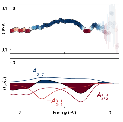
Figure 5: Comparison between experiment and DMFT. (a) $k_{z}$ integrated CPS ARPES data at normal emission. (b) LDA+DMFT calculations for Sr₂IrO₄ with Coulomb parameters $U=3.2$ eV and $J=0.4$ eV. Bare lines correspond to diagonal elements $A_{j,m_{j}}({\bf k};\omega)$ of the spin-orbital resolved spectral function in the $j$ basis at the $\Gamma$ point. The filled colored curve shows the calculated $\expectationvalue{L_{z}S_{z}}$.

$$\hat{H}= -\sum_{ii^{\prime}}\sum_{mm^{\prime}}\sum_{\sigma\sigma^{\prime}}t_{m\sigma,m^{\prime}\sigma^{\prime}}^{i,i^{\prime}}\hat{c}_{im\sigma}^{\dagger}\hat{c}_{i^{\prime}m^{\prime}\sigma^{\prime}}$$ (12)

$$+\frac{1}{2}\sum_{i}\sum_{mm^{\prime}pp^{\prime}}\sum_{\sigma\sigma^{\prime}}U_{mm^{\prime}pp^{\prime}}\hat{c}_{im\sigma}^{\dagger}\hat{c}_{im^{\prime}\sigma^{\prime}}^{\dagger}\hat{c}_{ip^{\prime}\sigma^{\prime}}\hat{c}_{ip\sigma}.$$

In the Hamiltonian above, $\hat{c}_{im\sigma}^{\dagger}$ ($\hat{c}_{im\sigma}$) creates (annihilates) an electron at lattice site $i$ with spin $\sigma\in\{\uparrow,\downarrow\}$ and orbital $m\in\{xy,yz,xz\}$. The parameters $-t_{m\sigma,m^{\prime}\sigma^{\prime}}^{i,i}$ define the on-site crystal-field matrix, including local spin-orbit terms; the intersite ($i\neq i^{\prime}$) terms $-t_{m\sigma,m^{\prime}\sigma^{\prime}}^{i,i^{\prime}}$ are the hopping integrals, also with spin-orbit interaction contributions. The key screened Coulomb integrals are the direct Coulomb interaction, $U_{mm^{\prime}mm^{\prime}}=U_{m,m^{\prime}}=U-2J(1-\delta_{m,m^{\prime}})$, the exchange Coulomb interaction $U_{mm^{\prime}m^{\prime}m}=J$, the pair-hopping term, $U_{mmm^{\prime}m^{\prime}}=J$, and the spin-flip term $U_{mm^{\prime}m^{\prime}m}=J$. We adopt the values $(U,J)=(3.2,0.4)$ eV, corresponding to an average Coulomb repulsion of $U_{\rm avg}=2.4$ eV; this reproduces the small insulating gap well, as we have shown in Ref. [34]. We solve (12) with DMFT using the interaction-expansion continuous time quantum Monte Carlo impurity solver, in the implementation developed in Refs. 35, 36, 37. The calculations presented have been performed at the electronic temperature 290K. We obtain the orbital and ${\bf k}$-resolved spectral-function matrix using the maximum-entropy method. In Fig. 4 we show the weight of each component along high-symmetry lines if the Brillouin Zone. The $k_{z}$ dispersion itself is small and difficult to resolve, but the shift in character with energy is very clear at any k point. From here we calculate

$${\cal A}_{\langle L_{z}S_{z}\rangle} =\frac{1}{4}\bigg{(}A_{1,1}^{\uparrow}+A_{-1,-1}^{\downarrow}-A_{1,1}^{\downarrow}-A_{-1,-1}^{\uparrow}\bigg{)}$$ (13)

where $A_{m,m}^{\sigma}$ is the spectral function for orbital $m$ and spin $\sigma$. In the basis of the $j=1/2$ and $j=3/2$ states

$${\cal A}_{\langle L_{z}S_{z}\rangle} =-\frac{1}{2}A_{\frac{3}{2};\frac{3}{2}}+\frac{1}{6}A_{\frac{3}{2};\frac{1}{2}}+\frac{1}{3}A_{\frac{1}{2};\frac{1}{2}}+\frac{\sqrt{2}}{{3}}B_{\frac{3}{2},\frac{1}{2};\frac{1}{2}},$$ (14)

where $A_{j;m_{j}}$ are the diagonal elements of the spectral-function matrix in the $j$ basis, while $B_{j,j^{\prime};m_{j}}$ is an off-diagonal element ($j=j^{\prime}\pm 1/2,m_{j}=m_{j^{\prime}}=1/2$); the latter turns out to be small at low energy.

This provides a full description of the $t_{2g}$ manifold, which can recover a pseudo-spin 1/2 system as a special case, but covers a broader class of potential models. Such models combined with photoemission have previously been used to gain significant understanding of Sr₂RuO₄, which shares a similar amount of complexity associated with its low energy structure [36, 38]. The measured CPS ARPES intensity is proportional to ${\cal A}_{\langle L_{z}S_{z}\rangle}$. Along $\Gamma\mathrm{Z}$, only $A_{\frac{3}{2};\frac{3}{2}}$ and $A_{\frac{1}{2};\frac{1}{2}}$ contribute sizably at very low energy, and thus determine the sign of ${\cal A}_{\langle L_{z}S_{z}\rangle}$. Since the small $k_{z}$ dispersion is hard to resolve in our DMFT calculations, for a quantitative analysis in Fig. 5 we compare the DMFT results to CPS-ARPES spectra integrated over the $k_{z}$ axis, finding excellent agreement. Barring the precise energies where the sign of $\expectationvalue{L_{z}S_{z}}$ changes, all the positive and negative regions – including the unexpected negative peak around $E=-0.5$ eV – are reproduced (and in fact the quantitative agreement for the oscillating character of $\expectationvalue{L_{z}S_{z}}$ can be observed, not only for the lowest energy states, but on the full 4 eV energy window probed in the experiment). All the oscillations are present in both panels, which implies that DMFT gives an accurate representation of the band structure of Sr₂IrO₄.

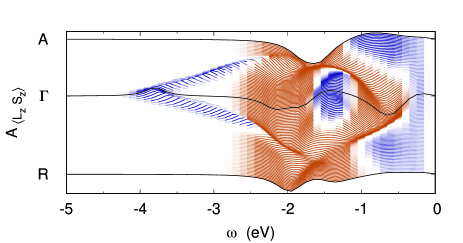
Figure 6: Evolution of $\expectationvalue{L_{z}S_{z}}$ along the directions $\Gamma-A$ and $\Gamma-R$, where $A=(\pi/a,\pi/a,\pi/c)$ and $R=(0,\pi/a,\pi/c)$.

It is worth pointing out that, although the exact energy where the sign changes deviates, the presence of these oscillations itself is independent of the precise values of the Coulomb parameters $U$ and $J$, or often adopted approximations of the Coulomb vertex, provided that they yield an insulating state. This further supports our conclusion that taking into account the multi-band nature of the system is the critical starting point. Our DMFT calculations give us direct access to the projections onto the $j_{1/2}$ and $j_{3/2}$ states (shown as bare lines in Fig. 5), allowing us to make more substantiated comments about our earlier claims: the spectral weight in the low energy states arises approximately for 74% from $j_{3/2}$ states, determined as the ratio of spectral weights integrated from the sign change in $\expectationvalue{L_{z}S_{z}}$ at $E=-1.64$ eV all the way up to $E=0$ eV.

The results obtained along ${\Gamma}\mathrm{A}$ and $\Gamma\mathrm{R}$ are shown in Fig. 6; away from the $\Gamma\mathrm{Z}$ direction. Since these results are presented away from “normal emission”, to compare these directly to experiments (i.e Fig. 7), a more advanced treatment of the photoemission dipole matrix elements is required. From these plots, we can see that towards the zone boundaries, the overall magnitude of $\expectationvalue{L_{z}S_{z}}$ decreases, as we observe in Fig. 7, and has also been suggested in [21] on the basis of density functional theory calculations.

V Conclusions

With our experiments and accompanying DMFT analysis we have thus demonstrated that a pseudo-spin 1/2 model is insufficient to give a satisfying description of the system at hand. Rather, one needs to rely on a modeling in terms of at least the full $t_{2g}$ states and electron-electron interactions. While a description in terms of $j_{1/2}$ orbitals was instrumental in developing our initial understanding of Sr₂IrO₄ and of why spin orbit coupling gives rise to an insulating ground state [5, 39], it is clear that this model lacks the descriptive power needed to make further reaching conclusions; especially connections made to the superconducting cuprates should be reevaluated in this light. Finally, and most importantly, we have demonstrated that with a carefully crafted combination of a sufficiently complete many-body computational framework and state-of-the-art experimental approaches, we can make tangible progress in understanding materials with closely intertwined energy scales such as Sr₂IrO₄.

Appendix A Effective $j$ states

The $j_{\mathrm{eff}}$ states arise from the similarities the $t_{2g}$ orbitals share with the $p$ orbitals, in particular with relation to spin-orbit coupling. We will construct the Hamiltonian, for which we first define the $t_{2g}$ basis:

$$b_{t_{2g}}=\left\{d_{xy,\uparrow},d_{xz,\uparrow},d_{yz,\uparrow},d_{xy,\downarrow},d_{xz,\downarrow},d_{yz,\downarrow}\right\},$$ (15)

we get for the $H_{SOC}$:

$$H_{SOC,t_{2g}}=\frac{\lambda}{2}\begin{pmatrix}0&0&0&0&-i&1\\ 0&0&-i&i&0&0\\ 0&i&0&-1&0&0\\ 0&-i&-1&0&0&0\\ i&0&0&0&0&i\\ 1&0&0&0&-i&0\\ \end{pmatrix}.$$ (16)

We then consider a transformation to a new basis of “effective” $m_{l}\in\{-1,0,1\}$ (reminiscent of $p$) orbitals, which we define as:

$$\ket{1_{\mathrm{eff}}}=\frac{1}{\sqrt{2}}\left(\ket{d_{yz}}+i\ket{d_{xz}}\right)=i\ket{Y^{-1}_{2}},$$ (17)

$$\ket{0_{\mathrm{eff}}}=-\ket{d_{xy}}=-\frac{i}{\sqrt{2}}\left(\ket{Y^{-2}_{2}}-\ket{Y^{2}_{2}}\right),$$ (18)

$$\ket{-1_{\mathrm{eff}}}=\frac{1}{\sqrt{2}}\left(-\ket{d_{yz}}+i\ket{d_{xz}}\right)=-i\ket{Y^{1}_{2}}.$$ (19)

Within this basis, the $L^{+}$ and $L_{z}$ operators become:

$$L^{+}_{l_{\mathrm{eff}}}=B_{l_{\mathrm{eff}}}^{-1}L^{+}B_{l_{\mathrm{eff}}}=\sqrt{2}\begin{pmatrix}0&-1&0\\ 0&0&-1\\ 0&0&0\\ \end{pmatrix},$$ (20)

$$L_{z,{l_{\mathrm{eff}}}}=B_{l_{\mathrm{eff}}}^{-1}L_{z}B_{l_{\mathrm{eff}}}=\begin{pmatrix}-1&0&0\\ 0&0&0\\ 0&0&1\\ \end{pmatrix}.$$ (21)

These are identical to the respective matrices for the $\ell=1$ orbitals, except they are multiplied by $-1$, and thus behaving effectively as $\ell=-1$ states. If we use these $\ell=-1$ states to construct spin-orbit entangled states known as the $j_{\mathrm{eff}}$ states, as was first proposed in [5], we obtain as the spin-orbit coupling Hamiltonian:

$$H_{SOC,j_{\mathrm{eff}}}=\begin{pmatrix}1&0&0&0&0&0\\ 0&1&0&0&0&0\\ 0&0&-\frac{1}{2}&0&0&0\\ 0&0&0&-\frac{1}{2}&0&0\\ 0&0&0&0&-\frac{1}{2}&0\\ 0&0&0&0&0&-\frac{1}{2}\\ \end{pmatrix}.$$ (22)

This is again equal to the spin-orbit coupling Hamiltonian for $\ell=1$ states, up to a minus sign. To this end, the expectation values $\expectationvalue{\mathbf{L}\cdot\mathbf{S}}$ are negative to what is expected from “regular” $j$-states.

Appendix B Further CPS background

B.1 Data taken away from normal emission

So far, the only expectation value discussed is the one along the $z$ direction, and the calculated expectation values are only valid at the $\Gamma$-point. Despite this, the technique has been successfully applied away from $\Gamma$ [28]. The equations hold true as long as not too much weight comes from final states with $m_{l}\neq 0$. Following the $k$-dependent spherical harmonic in Eq. 1, these other components have a dependence $\propto\left(1-\cos^{2}\theta_{k}\right)$, where $\theta_{k}$ is the angle of the photoemitted electron and the surface normal. In particular, if the photon energy is large, this angle is relatively small.

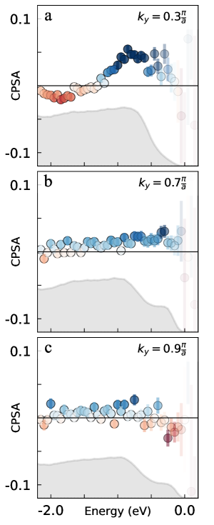
Figure 7: (a-c) Measurement of the CPS ARPES signal through the Brillouin zone (colored markers) and spin-integrated signal (grey line).

B.2 Polarization of the incoming light

The calculations presented up to this point have assumed that the incident light is perfectly perpendicular to the surface. In the geometry of a realistic ARPES experiment, the electron analyzer would be in the light path. Therefore, the incidence angle of the light is usually approximately 45^∘. We will investigate here what effect of such an incidence angle is on the final spectrum.
Taking the direction of the sample surface normal to be $\hat{\mathbf{z}}$, we can write for the incoming light:

$$\bm{\varepsilon}^{\oplus}=\varepsilon_{0}\left(\frac{1}{\sqrt{4}}\left(\hat{\mathbf{x}}-\hat{\mathbf{z}}\right)+i\hat{\mathbf{y}}\right).$$ (23)

This can be converted into spherical harmonics, for which we can easily read off the equivalent normal incidence light parameters:

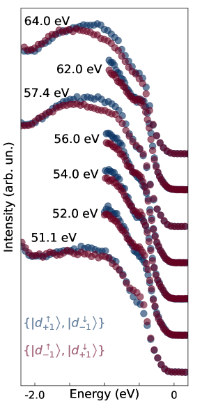
Figure 8: Photon energy dependent CPS ARPES measurements, plots of the parallel (blue) and antiparallel (red) signal.

$$\bm{\varepsilon}^{\oplus}=\frac{1}{\sqrt{4}}Y^{0}_{1}+(\frac{1}{\sqrt{4}}+\frac{1}{\sqrt{8}})Y^{1}_{1}+(\frac{1}{\sqrt{4}}-\frac{1}{\sqrt{8}})Y^{-1}_{1}.$$ (24)

This deviates from the ideal case where we only make excitations with $Y^{1}_{1}$. However, at $\Gamma$, there are no available final state channels for $Y^{0}_{1}$ to scatter into. At finite emission angles $\theta$ this will generate a small unpolarized contribution that grows as $1-\cos^{2}\theta$. The $Y^{-1}_{1}$ term meanwhile creates excitations of the opposite spin-orbital entanglement. Taking the squares of these coefficients, we get $0.73$, and for $0.02$ for $Y^{1}_{1}$ and $Y^{-1}_{1}$ respectively. This means that this configuration leads to an opposite signal of just 3% at normal emission, generating a net 6% of additional, unpolarized signal. This is far less than the approximate Sherman function [30], which is around 50% for the (high-efficiency) VLEED detectors we have used for our measurements. We can therefore safely ignore the angle of the incoming light.

Appendix C Additional CPS data

C.1 In-plane $k$-dependent CPS ARPES data

To identify how the spin-orbital entanglement changes throughout the Brillouin zone, we present CPS ARPES measurements at various points along the $(0,0)-(0,\pi)$ direction in Fig. 7. Going away from the $\Gamma$ point, the CPS ARPES signal rapidly diminishes until the signal completely vanishes at the zone boundary. Similar observations are made if the measurements are taken along the $(0,0)-(\pi,0)$ direction (not shown), confirming the reliability of the measurement in this $C_{4}$ symmetric system. Previous work has suggested that the coupling into $j_{\mathrm{eff}}$ states is strongest at $\Gamma$, while hopping terms have a larger influence at the zone boundaries [21], which is consistent with our observations. These data support the interpretation that the spin-orbital entanglement varies through $k$-space, and in fact reduces toward the zone boundary.

C.2 Individual components of the CPS ARPES signal

In order to better understand what regions in energy the features in the CPS ARPES spectra arise, it is insightful to plot the parallel (${\{\ket{d_{+1}^{\uparrow}},\ket{d_{-1}^{\downarrow}}\}}$) and anti-parallel (${\{\ket{d_{-1}^{\uparrow}},\ket{d_{+1}^{\downarrow}}\}}$) components of the spectrum, defined as:

$$I_{\{\ket{d_{+1}^{\uparrow}},\ket{d_{-1}^{\downarrow}}\}} =\sqrt{I_{\uparrow}^{\ominus}I_{\downarrow}^{\oplus}}$$ (25)

$$I_{\{\ket{d_{-1}^{\uparrow}},\ket{d_{+1}^{\downarrow}}\}} =\sqrt{I_{\downarrow}^{\ominus}I_{\uparrow}^{\oplus}},$$ (26)

which together form the CPS ARPES signal as defined in the main text. These signals are plotted in Fig. 8 in blue ($I_{\{\ket{d_{+1}^{\uparrow}},\ket{d_{-1}^{\downarrow}}\}}$) and red ($I_{\{\ket{d_{-1}^{\uparrow}},\ket{d_{+1}^{\downarrow}}\}}$) for the same photon energies as presented in Fig. 3 in the main text. From these spectra it is straightforward to see that the sign-changing signal in $k_{z}$ arises from the state that appears as a shoulder around $E=-0.5$ eV.

References

- Bednorz and Müller [1986] J. G. Bednorz and K. A. Müller, Zeitschrift für Physik B Condensed Matter 64, 189 (1986).
- Cava et al. [1994] R. J. Cava, B. Batlogg, K. Kiyono, H. Takagi, J. J. Krajewski, W. F. Peck, L. W. Rupp, and C. H. Chen, Phys. Rev. B 49, 11890 (1994).
- Crawford et al. [1994] M. K. Crawford, M. A. Subramanian, R. L. Harlow, J. A. Fernandez-Baca, Z. R. Wang, and D. C. Johnston, Phys. Rev. B 49, 9198 (1994).
- Cao et al. [1998] G. Cao, J. Bolivar, S. McCall, J. E. Crow, and R. P. Guertin, Phys. Rev. B 57, R11039 (1998).
- Kim et al. [2008] B. J. Kim, H. Jin, S. J. Moon, J.-Y. Kim, B.-G. Park, C. S. Leem, J. Yu, T. W. Noh, C. Kim, S.-J. Oh, J.-H. Park, V. Durairaj, G. Cao, and E. Rotenberg, Phys. Rev. Lett. 101, 076402 (2008).
- Wang and Senthil [2011] F. Wang and T. Senthil, Phys. Rev. Lett. 106, 136402 (2011).
- Watanabe et al. [2013] H. Watanabe, T. Shirakawa, and S. Yunoki, Phys. Rev. Lett. 110, 027002 (2013).
- Meng et al. [2014] Z. Y. Meng, Y. B. Kim, and H.-Y. Kee, Phys. Rev. Lett. 113, 177003 (2014).
- Kim et al. [2012a] B. H. Kim, G. Khaliullin, and B. I. Min, Phys. Rev. Lett. 109, 167205 (2012a).
- Kim et al. [2012b] J. Kim, D. Casa, M. H. Upton, T. Gog, Y.-J. Kim, J. F. Mitchell, M. van Veenendaal, M. Daghofer, J. van den Brink, G. Khaliullin, and B. J. Kim, Phys. Rev. Lett. 108, 177003 (2012b).
- Kastner et al. [1998] M. A. Kastner, R. J. Birgeneau, G. Shirane, and Y. Endoh, Rev. Mod. Phys. 70, 897 (1998).
- J. Birgeneau et al. [2006] R. J. Birgeneau, C. Stock, J. M. Tranquada, and K. Yamada, J. Phys. Soc. Jpn. 75, 111003 (2006), https://doi.org/10.1143/JPSJ.75.111003 .
- Battisti et al. [2016] I. Battisti, K. M. Bastiaans, V. Fedoseev, A. de la Torre, N. Iliopoulos, A. Tamai, E. C. Hunter, R. S. Perry, J. Zaanen, F. Baumberger, and M. P. Allan, Nat. Phys. 13, 21 (2016).
- de la Torre et al. [2015] A. de la Torre, S. McKeown Walker, F. Y. Bruno, S. Riccó, Z. Wang, I. Gutierrez Lezama, G. Scheerer, G. Giriat, D. Jaccard, C. Berthod, T. K. Kim, M. Hoesch, E. C. Hunter, R. S. Perry, A. Tamai, and F. Baumberger, Phys. Rev. Lett. 115, 176402 (2015).
- Yan et al. [2015] Y. J. Yan, M. Q. Ren, H. C. Xu, B. P. Xie, R. Tao, H. Y. Choi, N. Lee, Y. J. Choi, T. Zhang, and D. L. Feng, Phys. Rev. X 5, 041018 (2015).
- Kim et al. [2015] Y. K. Kim, N. H. Sung, J. D. Denlinger, and B. J. Kim, Nat. Phys. 12 (2015), 10.1038/nphys3503.
- Mattheiss [1976] L. F. Mattheiss, Phys. Rev. B 13, 2433 (1976).
- Moon et al. [2008] S. J. Moon, H. Jin, K. W. Kim, W. S. Choi, Y. S. Lee, J. Yu, G. Cao, A. Sumi, H. Funakubo, C. Bernhard, and T. W. Noh, Phys. Rev. Lett. 101, 226402 (2008).
- Brouet et al. [2015] V. Brouet, J. Mansart, L. Perfetti, C. Piovera, I. Vobornik, P. Le Fèvre, F. m. c. Bertran, S. C. Riggs, M. C. Shapiro, P. Giraldo-Gallo, and I. R. Fisher, Phys. Rev. B 92, 081117 (2015).
- Cao et al. [2016] Y. Cao, Q. Wang, J. A. Waugh, T. J. Reber, H. Li, X. Zhou, S. Parham, S.-R. Park, N. C. Plumb, E. Rotenberg, A. Bostwick, J. D. Denlinger, T. Qi, M. A. Hermele, G. Cao, and D. S. Dessau, Nat. Commun. 7, 11367 (2016).
- Louat et al. [2018] A. Louat, F. Bert, L. Serrier-Garcia, F. Bertran, P. Le Fèvre, J. Rault, and V. Brouet, Phys. Rev. B 97, 161109 (2018).
- Note [1] To reduce the notational clutter, we will henceforth refer to the and states as and respectively.
- Jeong et al. [2020] J. Jeong, B. Lenz, A. Gukasov, X. Fabrèges, A. Sazonov, V. Hutanu, A. Louat, D. Bounoua, C. Martins, S. Biermann, V. Brouet, Y. Sidis, and P. Bourges, Phys. Rev. Lett. 125, 097202 (2020).
- Note [2] Since the states are constructed from , the 1/2 (3/2) state has parallel (antiparallel) alignment of spin and orbital angular momentum. A more thorough review is presented in the appendix.
- Pierce and Meier [1976] D. T. Pierce and F. Meier, Phys. Rev. B 13, 5484 (1976).
- Mizokawa et al. [2001] T. Mizokawa, L. H. Tjeng, G. A. Sawatzky, G. Ghiringhelli, O. Tjernberg, N. B. Brookes, H. Fukazawa, S. Nakatsuji, and Y. Maeno, Phys. Rev. Lett. 87, 077202 (2001).
- Veenstra et al. [2014] C. N. Veenstra, Z.-H. Zhu, M. Raichle, B. M. Ludbrook, A. Nicolaou, B. Slomski, G. Landolt, S. Kittaka, Y. Maeno, J. H. Dil, I. S. Elfimov, M. W. Haverkort, and A. Damascelli, Phys. Rev. Lett. 112, 127002 (2014).
- Day et al. [2018] R. P. Day, G. Levy, M. Michiardi, B. Zwartsenberg, M. Zonno, F. Ji, E. Razzoli, F. Boschini, S. Chi, R. Liang, P. K. Das, I. Vobornik, J. Fujii, W. N. Hardy, D. A. Bonn, I. S. Elfimov, and A. Damascelli, Phys. Rev. Lett. 121, 076401 (2018).
- Day et al. [2019] R. P. Day, B. Zwartsenberg, I. S. Elfimov, and A. Damascelli, npj Quantum Materials 4, 54 (2019).
- Bigi et al. [2017] C. Bigi, P. K. Das, D. Benedetti, F. Salvador, D. Krizmancic, R. Sergo, A. Martin, G. Panaccione, G. Rossi, J. Fujii, and I. Vobornik, Journal of Synchrotron Radiation 24, 750 (2017).
- Wang et al. [2013] Q. Wang, Y. Cao, J. A. Waugh, S. R. Park, T. F. Qi, O. B. Korneta, G. Cao, and D. S. Dessau, Phys. Rev. B 87, 245109 (2013).
- Damascelli [2004] A. Damascelli, Phys. Scr. T109, 61 (2004).
- Blaha et al. [2018] P. Blaha, K. Schwarz, G. K. H. Madsen, D. Kvasnicka, J. Luitz, R. Laskowski, F. Tran, and M. Laurence D., WIEN2k, An Augmented Plane Wave + Local Orbitals Program for Calculating Crystal Properties (Karlheinz Schwarz, Techn. Universität Wien, Austria, 2018).
- Zhang and Pavarini [2021] G. Zhang and E. Pavarini, Phys. Rev. B 104, 125116 (2021).
- Gorelov et al. [2010] E. Gorelov, M. Karolak, T. O. Wehling, F. Lechermann, A. I. Lichtenstein, and E. Pavarini, Phys. Rev. Lett. 104, 226401 (2010).
- Zhang et al. [2016] G. Zhang, E. Gorelov, E. Sarvestani, and E. Pavarini, Phys. Rev. Lett. 116, 106402 (2016).
- Zhang and Pavarini [2017] G. Zhang and E. Pavarini, Phys. Rev. B 95, 075145 (2017).
- Kim et al. [2018] M. Kim, J. Mravlje, M. Ferrero, O. Parcollet, and A. Georges, Phys. Rev. Lett. 120, 126401 (2018).
- Zwartsenberg et al. [2020] B. Zwartsenberg, R. P. Day, E. Razzoli, M. Michiardi, N. Xu, M. Shi, J. D. Denlinger, G. Cao, S. Calder, K. Ueda, J. Bertinshaw, H. Takagi, B. J. Kim, I. S. Elfimov, and A. Damascelli, Nature Physics 16, 290 (2020).