Recipe for a General, Powerful, Scalable
Graph Transformer

Abstract

We propose a recipe on how to build a general, powerful, scalable (GPS) graph Transformer with linear complexity and state-of-the-art results on a diverse set of benchmarks. Graph Transformers (GTs) have gained popularity in the field of graph representation learning with a variety of recent publications but they lack a common foundation about what constitutes a good positional or structural encoding, and what differentiates them. In this paper, we summarize the different types of encodings with a clearer definition and categorize them as being local, global or relative. The prior GTs are constrained to small graphs with a few hundred nodes, here we propose the first architecture with a complexity linear in the number of nodes and edges $O(N+E)$ by decoupling the local real-edge aggregation from the fully-connected Transformer. We argue that this decoupling does not negatively affect the expressivity, with our architecture being a universal function approximator on graphs. Our GPS recipe consists of choosing 3 main ingredients: (i) positional/structural encoding, (ii) local message-passing mechanism, and (iii) global attention mechanism. We provide a modular framework GraphGPS that supports multiple types of encodings and that provides efficiency and scalability both in small and large graphs. We test our architecture on 16 benchmarks and show highly competitive results in all of them, show-casing the empirical benefits gained by the modularity and the combination of different strategies.

1 Introduction

Graph Transformers (GTs) alleviate fundamental limitations pertaining to the sparse message passing mechanism, e.g., over-smoothing [47], over-squashing [1], and expressiveness bounds [61, 45], by allowing nodes to attend to all other nodes in a graph (global attention). This benefits several real-world applications, such as modeling chemical interactions beyond the covalent bonds [63], or graph-based robotic control [37]. Global attention, however, requires nodes to be better identifiable within the graph and its substructures [14]. This has led to a flurry of recently proposed fully-connected graph transformer models [14, 36, 63, 44, 31] as well as various positional encoding schemes leveraging spectral features [14, 36, 39] and graph features [16, 9]. Furthermore, standard global attention incurs quadratic computational costs $O(N^{2})$ for a graph with $N$ nodes and $E$ edges, that limits GTs to small graphs with up to a few hundred nodes.

Whereas various GT models focus on particular node identifiability aspects, a principled framework for designing GTs is still missing. In this work, we address this gap and propose a recipe for building general, powerful, and scalable (GPS) graph Transformers. The recipe defines (i) embedding modules responsible for aggregating positional encodings (PE) and structural encodings (SE) with the node, edge, and graph level input features; (ii) processing modules that employ a combination of local message passing and global attention layers (see Figure 1).

The embedding modules organize multiple proposed PE and SE schemes into local and global levels serving as additional node features whereas positional and structural relative features contribute to edge features. The processing modules define a computational graph that allows to balance between message-passing graph neural networks (MPNNs) and Transformer-like global attention, including attention mechanisms linear in the number of nodes $O(N)$.

To the best of our knowledge, application of efficient attention models has not yet been thoroughly studied in the graph domain, e.g., only one work [11] explores the adaptation of Performer-style [12] attention approximation on small graphs. Particular challenges emerge with explicit edge features that are incorporated as attention bias in fully-connected graph transformers [36, 63]. Linear transformers do not materialize the attention matrix directly, hence incorporating edge features becomes a non-trivial task. In this work, we hypothesize that explicit edge features are not necessary for the global graph attention and adopt Performer [12] and BigBird [66] as exemplary linear attention mechanisms.

Our contributions are as follows. (i) Provide a general, powerful, scalable (GPS) GT blueprint that incorporates positional and structural encodings with local message passing and global attention, visualized in Figure 1. (ii) Provide a better definition of PEs and SEs and organize them into local, global, and relative categories. (iii) Show that GPS with linear global attention, e.g., provided by Performer [12] or BigBird [66], scales to graphs with several thousand nodes and demonstrates competitive results even without explicit edge features within the attention module, whereas existing fully-connected GTs [36, 63] are limited to graphs of up to few hundred nodes. (iv) Conduct an extensive ablation study that evaluates contribution of PEs, local MPNN, and global attention components in perspective of several benchmarking datasets. (v) Finally, following the success of GraphGym [65] we implement the blueprint within a modular and performant GraphGPS package.

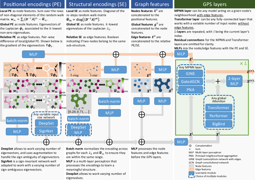
Figure 1: Modular GPS graph Transformer, with examples of PE and SE. Task specific layers for node/graph/edge-level predictions, such as pooling or output MLP, are omitted for simplicity.

2 Related Work

Graph Transformers (GT). Considering the great successes of Transformers in natural language processing (NLP) [55, 32] and recently also in computer vision [18, 25, 24], it is natural to study their applicability in the graph domain as well. Particularly, they are expected to help alleviate the problems of over-smoothing and over-squashing [1, 54] in MPNNs, which are analogous to the vanishing gradients and lack of long-term dependencies in NLP. Fully-connected Graph Transformer [14] was first introduced together with rudimentary utilisation of eigenvectors of the graph Laplacian as the node positional encoding (PE), to provide the otherwise graph-unaware Transformer a sense of nodes’ location in the input graph. Building on top of this work, SAN [36] implemented an invariant aggregation of Laplacian’s eigenvectors for the PE, alongside conditional attention for real and virtual edges of a graph, which jointly yielded significant improvements. Concurrently, Graphormer [63, 51] proposed using pair-wise graph distances (or 3D distances) to define relative positional encodings, with outstanding success on large molecular benchmarks. Further, GraphiT [44] used relative PE derived from diffusion kernels to modulate the attention between nodes. Finally, GraphTrans [31] proposed the first hybrid architecture, first using a stack of MPNN layers, before fully-connecting the graph. Since, the field has continued to propose alternative GTs: SAT [9], EGT [29], GRPE [48].

Positional and structural encodings. There have been many recent works on PE and SE, notably on Laplacian PE [14, 36, 3, 57, 39], shortest-path-distance [38, 63], node degree centrality [63], kernel distance [44], random-walk SE [16], structure-aware [9, 6, 5], and more. Some works also propose dedicated networks to learn the PE/SE from an initial encoding [36, 16, 39, 9]. To better understand the different PE/SE and the contribution of each work, we categorize them in Table 1 and examine their effect in Section 3.2. In most cases, PE/SE are used as soft bias, meaning they are simply provided as input features. But in other cases, they can be used to direct the messages [3] or create bridges between distant nodes [35, 54].

Linear Transformers. The quadratic complexity of attention in the original Transformer architecture [55] motivated the search for more efficient attention mechanisms that would scale linearly with the sequence length. Most of such linear transformers are developed for language modeling tasks, e.g., Linformer [58], Reformer [34], Longformer [4], Performer [12], BigBird [66], and have a dedicated Long Range Arena benchmark [52] to study the limits of models against extremely long input sequences. Pyraformer [40] is an example of a linear transformer for time series data, whereas S4 [23] is a more general signal processing approach that employs the state space model theory without the attention mechanism. In the graph domain, linear transformers are not well studied. Choromanski et al. [11] are the first to adapt Performer-style attention kernelization to small graphs.

3 Methods

In this work we provide a general, powerful, scalable (GPS) architecture for graph Transformers, following our 3-part recipe presented in Figure 1. We begin by categorization of existing positional (PE) and structural encodings (SE), a necessary ingredient for graph Transformers. Next, we analyse how these encodings also increase expressive power of MPNNs. The increased expressivity thus provides double benefit to our hybrid MPNN+Transformer architecture, which we introduce in Section 3.3. Last but not least, we provide an extensible implementation of GPS in GraphGPS package, built on top of PyG [20] and GraphGym [65].

3.1 Modular positional and structural encodings

One of our contribution is to provide a modular framework for PE/SE. It was shown in previous works that they are one of the most important factors in driving the performance of graph Transformers. Thus, a better understanding and organization of the PE and SE will aid in building of a more modular architecture and in guiding of the future research.

We propose to organize the PE and SE into 3 categories: local, global and relative in order to facilitate the integration within the pipeline and facilitate new research directions. They are presented visually in Figure 1, with more details in Table 1. Although PE and SE can appear similar to some extent, they are different yet complementary. PE gives a notion of distance, while SE gives a notion of structural similarity. One can always infer certain notions of distance from large structures, or certain notions of structure from short distances, but this is not a trivial task, and the objective of providing PE and SE remains distinct, as discussed in the following subsections.

Despite presenting a variety of possible functions, we focus our empirical evaluations on the global PE, relative PE and local SE since they are known to yield significant improvements. We leave the empirical evaluation of other encodings for future work.

Positional encodings (PE) are meant to provide an idea of the position in space of a given node within the graph. Hence, when two nodes are close to each other within a graph or subgraph, their PE should also be close. A common approach is to compute the pair-wise distance between each pairs of nodes or their eigenvectors as proposed in [38, 63, 36, 57], but this is not compatible with linear Transformers as it requires to materialize the full attention matrix [12]. Instead, we want the PE to either be features of the nodes or real edges of the graph, thus a better fitting solution is to use the eigenvectors of the graph Laplacian or their gradient [15, 3, 36]. See Table 1 for more PE examples.

Table 1: The proposed categorization of positional encodings (PE) and structural encodings (SE). Some encodings are assigned to multiple categories in order to show their multiple expected roles.

Encoding type	Description	Examples
Local PE node features	Allow a node to know its position and role within a local cluster of nodes. Within a cluster, the closer two nodes are to each other, the closer their local PE will be, such as the position of a word in a sentence (not in the text).	• Sum each column of non-diagonal elements of the $m$-steps random walk matrix. • Distance between a node and the centroid of a cluster containing the node.
Global PE node features	Allow a node to know its global position within the graph. Within a graph, the closer two nodes are, the closer their global PE will be, such as the position of a word in a text.	• Eigenvectors of the Adjacency, Laplacian [15, 36] or distance matrices. • SignNet [39] (includes aspects of relative PE and local SE). • Distance from the graph’s centroid. • Unique identifier for each connected component of the graph.
Relative PE edge features	Allow two nodes to understand their distances or directional relationships. Edge embedding that is correlated to the distance given by any global or local PE, such as the distance between two words.	• Pair-wise node distances [38, 3, 36, 63, 44] based on shortest-paths, heat kernels, random-walks, Green’s function, graph geodesic, or any local/global PE. • Gradient of eigenvectors [3, 36] or any local/global PE. • PEG layer [57] with specific node-wise distances. • Boolean indicating if two nodes are in the same cluster.
Local SE node features	Allow a node to understand what sub-structures it is a part of. Given an SE of radius $m$, the more similar the $m$-hop subgraphs around two nodes are, the closer their local SE will be.	• Degree of a node [63]. • Diagonal of the $m$-steps random-walk matrix [16]. • Time-derivative of the heat-kernel diagonal (gives the degree at $t=0$). • Enumerate or count predefined structures such as triangles, rings, etc. [6, 68]. • Ricci curvature [54].
Global SE graph features	Provide the network with information about the global structure of the graph. The more similar two graphs are, the closer their global SE will be.	• Eigenvalues of the Adjacency or Laplacian matrices [36]. • Graph properties: diameter, girth, number of connected components, # of nodes, # of edges, nodes-to-edges ratio.
Relative SE edge features	Allow two nodes to understand how much their structures differ. Edge embedding that is correlated to the difference between any local SE.	• Pair-wise distance, encoding, or gradient of any local SE. • Boolean indicating if two nodes are in the same sub-structure [5] (similar to the gradient of sub-structure enumeration).

Structural encodings (SE) are meant to provide an embedding of the structure of graphs or subgraphs to help increase the expressivity and the generalizability of graph neural networks (GNN). Hence, when two nodes share similar subgraphs, or when two graphs are similar, their SE should also be close. Simple approaches are to identify pre-defined patterns in the graphs as one-hot encodings, but they require expert knowledge of graphs [6, 5]. Instead, using the diagonal of the $m$-steps random-walk matrix encodes richer information into each node [16], such as for odd $m$ it can indicate if a node is a part of an $m$-long cycle. Structural encodings can also be used to define the global graph structure, for instance using the eigenvalues of the Laplacian, or as relative edge features to identify if nodes are contained within the same clusters, with more examples in Table 1.

3.2 Why do we need PE and SE in MPNN?

As reviewed earlier, several recent GNNs make use of positional encodings (PE) and structural encodings (SE) as soft biases to improve the model expressivity (summarized in Table 1), which also leads to better generalization. In this section, we present an examination of PE and SE by showing how message-passing networks, despite operating on the graph structure, remain blind to the information encapsulated by the PE and SE.

1-Weisfeiler-Leman test (1-WL). It is well known that standard MPNNs are as expressive as the 1-WL test, meaning that they fail to distinguish non-isomorphic graphs under a 1-hop aggregation. We argue that the selected local, global and relative PE/SE allow MPNNs to become more expressive than the 1-WL test, thus making them fundamentally more expressive at distinguishing between nodes and graphs. To this end, we study the following two types of graphs (Figure 2 and Appendix C.1).

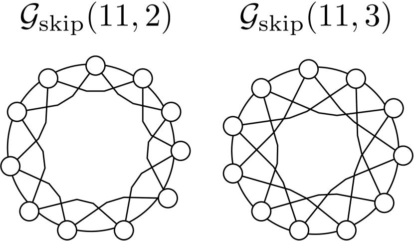
(a) Circular Skip Link graphs

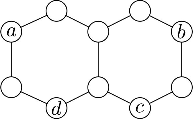
(b) Decalin molecular graph

Figure 2: Example graphs with anonymous nodes without distinguishing features.

Circular Skip Link (CSL) graph. In a CSL graph-pair [46], we want to be able to distinguish the two non-isomorphic graphs. Since the 1-WL algorithm produces the same color for every node in both graphs, also every MPNN will fail to distinguish them. However, using a global PE (e.g., Laplacian PE [15]) assigns each node a unique initial color and makes the CSL graph-pair distinguishable. This demonstrates that an MPNN cannot learn such a PE from the graph structure alone. Next, using a local SE (e.g., diagonals of $m$-steps random walk) can successfully capture the difference in the skip links of the two graphs [42], resulting in their different node coloring [16].

Decalin molecule. In the bicyclic Decalin graph, Figures 2(b) and 1(b), the node $a$ is isomorphic to node $b$, and so is the node $c$ to node $d$. A 1-WL coloring of the nodes, and analogously MPNN, would generate one color for the nodes $a,b$ and another color for $c,d$. The same applies to the aforementioned local SE [16]. In case of link prediction, this causes potential links $(a,d)$ and $(b,d)$ to be indistinguishable [67]. Using a distance-based relative PE on the edges or an eigenvector-based global PE, however, would allow to differentiate the two links.

3.3 GPS layer: an MPNN+Transformer hybrid

In this section we introduce the GPS layer, which is a hybrid MPNN+Transformer layer. First we argue how it alleviates the limitation of a closely related work. Next, we list the layer update equations which can be instantiated with a variety of MPNN and Transformer layers. Finally, we present its characteristics in terms of modularity, scalability and expressivity.

Preventing early smoothing. Why not use an architecture like GraphTrans [31] comprising of a few layers of MPNNs before the Transformer? Since MPNNs are limited by problems of over-smoothing, over-squashing, and low expressivity against the WL test [1, 54], these layers could irreparably fail to keep some information in the early stage. Although they could make use of PE/SE or more expressive MPNNs [3, 16], they are still likely to lose information. An analogous 2-stage strategy was successful in computer vision [18, 24] thanks to the high expressivity of convolutional layers on grids, but we do not expect it to achieve the same success on graphs due to the limitations of message-passing.

Update function. At each layer, the features are updated by aggregating the output of an MPNN layer with that of a global attention layer, as shown in Figures 1 and D.1, and described by the equations below. Note that the edge features are only passed to the MPNN layer, and that residual connections with batch normalization [30] are omitted for clarity. Both the MPNN and GlobalAttn layers are modular, i.e., MPNN can be any function that acts on a local neighborhood and GlobalAttn can be any fully-connected layer.

$$\mathbf{X}^{\ell+1},\mathbf{E}^{\ell+1} = \texttt{GPS}^{\ell}\left(\mathbf{X}^{\ell},\mathbf{E}^{\ell},\mathbf{A}\right)$$ (1)

$$\textrm{computed as}\ \ \ \ \mathbf{X}^{\ell+1}_{M},\ \mathbf{E}^{\ell+1} = \texttt{MPNN}_{e}^{\ell}\left(\mathbf{X}^{\ell},\mathbf{E}^{\ell},\mathbf{A}\right),$$ (2)

$$\mathbf{X}^{\ell+1}_{T} = \texttt{GlobalAttn}^{\ell}\left(\mathbf{X}^{\ell}\right),$$ (3)

$$\mathbf{X}^{\ell+1} = \texttt{MLP}^{\ell}\left(\mathbf{X}^{\ell+1}_{M}+\mathbf{X}^{\ell+1}_{T}\right),$$ (4)

where $\mathbf{A}\in\mathbb{R}^{N\times N}$ is the adjacency matrix of a graph with $N$ nodes and $E$ edges; $\mathbf{X}^{\ell}\in\mathbb{R}^{N\times d_{\ell}},\mathbf{E}^{\ell}\in\mathbb{R}^{E\times d_{\ell}}$ are the $d_{\ell}$-dimensional node and edge features, respectively; $\texttt{MPNN}_{e}^{\ell}$ and $\texttt{GlobalAttn}^{\ell}$ are instances of an MPNN with edge features and of a global attention mechanism at the $\ell$-th layer with their corresponding learnable parameters, respectively; $\texttt{MLP}^{\ell}$ is a 2-layer MLP block.

Modularity is achieved by allowing drop-in replacement for a number of module choices, including the initial PE/SE types, the networks that processes those PE/SE, the MPNN and global attention layers that constitute a GPS layer, and the final task-specific prediction head. Further, as research advances in different directions, GraphGPS allows to easily implement new PE/SE and other layers.

Scalability is achieved by allowing for a computational complexity linear in both the number of nodes and edges $O(N+E)$; excluding the potential precomputation step required for various PE, such as Laplacian eigen-decomposition. By restricting the PE/SE to real nodes and edges, and by excluding the edge features from the global attention layer, we can avoid materializing the full quadratic attention matrix. Therefore we can utilize a linear Transformer with $O(N)$ complexity, while the complexity of an MPNN is $O(E)$. For sparse graphs such as molecular graphs, regular graphs, and knowledge graphs, the edges are practically proportional to the nodes $E=\Theta(N)$, meaning the entire complexity can be considered linear in the number of nodes $O(N)$. Empirically, even on small molecular graphs, our architecture reduces computation time compared to other GT models, e.g., a model of ~6M parameters requires 196s per epoch on the ogbg-molpcba [27] dataset, compared to 883s for SAN [36] on the same GPU type.

Expressivity in terms of sub-structure identification and the Weisfeiler-Leman (WL) test is achieved via providing a rich set of PE/SE, as proposed in various works [3, 36, 16, 5, 6] and detailed in Section 3.1. Further, the Transformer allows to resolve the expressivity bottlenecks caused by over-smoothing [36] and over-squashing [1] by allowing information to spread across the graph via full-connectivity. Finally, in Section 3.4, we demonstrate that, given the right components, the proposed architecture does not lose edge information and is a universal function approximator on graphs.

3.4 Theoretical expressivity

In this section, we first discuss how the MPNN layer allows to propagate edge and neighbor information on the nodes. Then, we show that the proposed model is a universal function approximator on graphs, similarly to the SAN architecture [36].

Preserving edge information in the Transformer layer. Most GTs do not fully utilize edge features of the input graph. The Graph Transformer [14], SAN [36] and Graphormer [63] only use edge features to condition the attention between a pair of nodes, that is, they influence the attention gating mechanism but are not explicitly involved in updating of the node representations. GraphiT [44] does not consider edge features at all. Recent 2-step methods GraphTrans [31] and SAT [9] can use edge features in their first MPNN step, however this step is applied only once and typically includes several $k$ rounds of message passing. Therefore this latter approach may suffer from initial over-smoothing, as $k$-hop neighborhoods together with the respective edge features need to be represented in a fixed-sized node representation.

On the other hand, in GPS, interleaving one round of local neighborhood aggregation via an MPNN layer with global self-attention mechanism reduces the initial representation bottleneck and enables iterative local and global interactions. In the attention, the key-query-value mechanism only explicitly depends on the node features, but assuming efficient representation encoding by the MPNN, the node features can implicitly encode edge information, thus edges can play a role in either the key, query, or values. In Appendix C.2, we give a more formal argument on how, following an MPNN layer, node features can encode edge features alongside information related to node-connectivity.

Universal function approximator on graphs. Kreuzer et al. [36][Sec. 3.5] demonstrated the universality of graph Transformers. It was shown that, given the full set of Laplacian eigenvectors, the model was a universal function approximator on graphs and could provide an approximate solution to the isomorphism problem, making it more powerful than any Weisfeiler-Leman (WL) isomorphism test given enough parameters. Here, we argue that the same holds for our architecture since we can also use the full set of eigenvectors, and since all edge information can be propagated to the nodes.

4 Experiments

We perform ablation studies on 4 datasets to evaluate the contribution of the message-passing module, the global attention module, and the positional or structural encodings. Then, we evaluate GPS on a diverse set of 11 benchmarking datasets, and show state-of-the-art (SOTA) results in many cases.

We test on datasets from different sources to ensure diversity, providing their detailed description in Appendix A.1. From the Benchmarking GNNs [15], we test on the ZINC, PATTERN, CLUSTER, MNIST, CIFAR10. From the open graph benchmark (OGB) [27], we test on all graph-level datasets: ogbg-molhiv, ogbg-molpcba, ogbg-code2, and ogbg-ppa, and from their large-scale challenge we test on the OGB-LSC PCQM4Mv2 [28]. Finally, we also select MalNet-Tiny [21] with 5000 graphs, each of up to 5000 nodes, since the number of nodes provide a scaling challenge for Transformers.

4.1 Ablation studies

In this section, we evaluate multiple options for the three main components of our architecture in order to gauge their contribution to predictive performance and to better guide dataset-specific hyper-parameter optimization. First, we quantify benefits of the considered global-attention modules in 4 tasks. Then, we note that the MPNN layer is an essential part for high-performing models, and identify the layer type most likely to help. Finally, we observe when different global PE or local SE provide significant boost in the performance. All ablation results are averaged over multiple random seeds and summarized in Table 2, with additional information available in Appendix B.

Table 2: Summary of the ablation studies. Details of the architectural choices, parameters, standard deviation, and computation times are presented in Appendix B.

(c) Ablation of the Transformer and MPNN layers. We observe a major drop when using only a Transformer without an MPNN. Further, most datasets benefit from using a Transformer, without any negative impact.

Ablation			ZINC	PCQM4Mv2	CIFAR10	MalNet
				subset		-Tiny
			MAE $\downarrow$	MAE $\downarrow$	Acc. $\uparrow$	Acc. $\uparrow$
Global	Attention	none	0.070	0.1213	69.95	92.23
		Transformer	0.070	0.1159	72.31	93.50
		Performer	0.071	0.1142	70.67	92.64
		BigBird	0.071	0.1237	70.48	92.34
MPNN		none	0.217	0.3294	68.86	73.90
		GINE	0.070	0.1284	71.11	92.27
		GatedGCN	0.086	0.1159	72.31	92.64
		PNA	0.070	0.1409	73.42	91.67

(d) Ablation of the PE and SE types. RWSE provides consistent gains at relatively low computational cost, while SignNet^DeepSets is the single best performing encoding, albeit at increased computational cost.

Ablation		ZINC	PCQM4Mv2	CIFAR10	MalNet
			subset		-Tiny
		MAE $\downarrow$	MAE $\downarrow$	Acc. $\uparrow$	Acc. $\uparrow$
PE / SE	none	0.113	0.1355	71.49	92.64
	RWSE	0.070	0.1159	71.96	92.77
	LapPE	0.116	0.1201	72.31	92.74
	SignNetMLP	0.090	0.1158	71.74	92.57
	SignNetDeepSets	0.079	0.1144	72.37	93.13
	PEGLapEig	0.161	0.1209	72.10	92.27
*Encodings are color-coded by their positional or structural type.

Global-Attention module.

Here we consider global attention implemented as $O(N^{2})$ key-query-value Transformer attention or linear-time attention mechanisms of Performer or BigBird. We notice in Table 2(c) that using a Transformer is always beneficial, except for the ZINC dataset where no changes are observed. This motivates our architecture and the hypothesis that long-range dependencies are generally important. We further observe that Performer falls behind Transformer in terms of the predictive performance, although it provides a gain over the baseline and the ability to scale to very large graphs. Finally, BigBird in our setting offers no significant gain, while also being slower than Performer (see Appendix B).

Having no gain on the ZINC dataset is expected since the task is a combination of the computed octanol-water partition coefficient (cLogP) [60] and the synthetic accessibility score (SA-score) [19], both of which only count occurrences of local sub-structures. Hence, there is no need for a global connectivity, but a strong need for structural encodings.

Message-passing module.

Next, we evaluate the effect of various message-passing architectures, Table 2(c). It is apparent that they are fundamental to the success of our method: removing the layer leads to a significant drop in performance across all datasets. Indeed, without an MPNN, the edge features are not taken into consideration at all. Additionally, without reinforcing of the local graph structure, the network can overfit to the PE/SE. This reiterates findings of Kreuzer et al. [36], where considerably larger weights were assigned to the local attention.

We also find that although a vanilla PNA [13] generally outperforms GINE [26] and GatedGCN [7], adding the PE and SE results in major performance boost especially for the GatedGCN. This is consistent with results of Dwivedi et al. [16] and shows the importance of these encodings for gating.

Perhaps the necessity of a local message-passing module is due to the limited amount of graph data, and scaling to colossal datasets [49] that we encounter in language and vision could change that. Indeed, the Graphormer architecture [63] was able to perform very well on the full PCQM4Mv2 dataset without a local module. However, even large Transformer-based language models [8] and vision models [25] can benefit from an added local aggregation and outperform pure Transformers.

Positional/Structural Encodings.

Finally, we evaluate the effects of various PE/SE schemes, Table 2(d). We find them generally beneficial to downstream tasks, in concordance to the vast literature on the subject (see Table 1). The benefits of the different encodings are very dataset dependant, with the random-walk structural encoding (RWSE) being more beneficial for molecular data and the Laplacian eigenvectors encodings (LapPE) being more beneficial in image superpixels. However, using SignNet with DeepSets encoding [39] as an improved way of processing the LapPE seems to be consistently successful across tasks. We hypothesize that SignNet can learn structural representation using the eigenvectors, for example, to generate local heat-kernels that approximate random walks [2]. Last but not least we evaluate PEG-layer design [57] with Laplacian eigenmap.

4.2 Benchmarking GPS

We compare GPS against a set of popular message-passing neural networks (GCN, GIN, GatedGCN, PNA, etc.), graph transformers (SAN, Graphormer, etc.), and other recent graph neural networks with SOTA results (CIN, CRaWL, GIN-AK+, ExpC). To ensure diverse benchmarking tasks, we use datasets from Benchmarking-GNNs [15], OGB [27] and its large-scale challenge [28], and Long-Range Graph Benchmark [17], with more details given in Appendix A.1. We report the mean and standard deviation over 10 random seeds if not explicitly stated otherwise.

Table 3: Test performance in five benchmarks from [15]. Shown is the mean ± s.d. of 10 runs with different random seeds. Highlighted are the top first, second, and third results.

Model	ZINC	MNIST	CIFAR10	PATTERN	CLUSTER
	MAE $\downarrow$	Accuracy $\uparrow$	Accuracy $\uparrow$	Accuracy $\uparrow$	Accuracy $\uparrow$
GCN [33]	0.367 ± 0.011	90.705 ± 0.218	55.710 ± 0.381	71.892 ± 0.334	68.498 ± 0.976
GIN [61]	0.526 ± 0.051	96.485 ± 0.252	55.255 ± 1.527	85.387 ± 0.136	64.716 ± 1.553
GAT [56]	0.384 ± 0.007	95.535 ± 0.205	64.223 ± 0.455	78.271 ± 0.186	70.587 ± 0.447
GatedGCN [7, 15]	0.282 ± 0.015	97.340 ± 0.143	67.312 ± 0.311	85.568 ± 0.088	73.840 ± 0.326
GatedGCN-LSPE [16]	0.090 ± 0.001	–	–	–	–
PNA [13]	0.188 ± 0.004	97.94 ± 0.12	70.35 ± 0.63	–	–
DGN [3]	0.168 ± 0.003	–	72.838 ± 0.417	86.680 ± 0.034	–
GSN [6]	0.101 ± 0.010	–	–	–	–
CIN [5]	0.079 ± 0.006	–	–	–	–
CRaWl [53]	0.085 ± 0.004	97.944 ± 0.050	69.013 ± 0.259	–	–
GIN-AK+ [68]	0.080 ± 0.001	–	72.19 ± 0.13	86.850 ± 0.057	–
SAN [36]	0.139 ± 0.006	–	–	86.581 ± 0.037	76.691 ± 0.65
Graphormer [63]	0.122 ± 0.006	–	–	–	–
K-Subgraph SAT [9]	0.094 ± 0.008	–	–	86.848 ± 0.037	77.856 ± 0.104
EGT [29]	0.108 ± 0.009	98.173 ± 0.087	68.702 ± 0.409	86.821 ± 0.020	79.232 ± 0.348
GPS (ours)	0.070 ± 0.004	98.051 ± 0.126	72.298 ± 0.356	86.685 ± 0.059	78.016 ± 0.180

Benchmarking GNNs [15]. We first benchmark our method on 5 tasks from Benchmarking GNNs [15], namely ZINC, MNIST, CIFAR10, PATTERN, and CLUSTER, shown in Table 3. We observe that our GPS gives SOTA results on ZINC and the second best in 3 more datasets, showcasing the ability to perform very well on a variety of synthetic tasks designed to test the model expressivity.

Open Graph Benchmark [27]. Next, we benchmark on all 4 graph-level tasks from OGB, namely molhiv, molpcba, ppa, and code2, Table 4. On the molhiv dataset, we observed our model to suffer from overfitting, but to still outperform SAN, while other graph Transformers do not report results. For the molpcba, ppa, and code2, GPS always ranks among the top 3 models, highlighting again the versatility and expressiveness of the GPS approach. Further, GPS outperforms every other GT on all 4 benchmarks, except SAT on code2.

OGB-LSC PCQM4Mv2 [28]. The large-scale PCQM4Mv2 dataset has been a popular benchmark for recent GTs, particularly due to Graphormer [63] winning the initial challenge. We report the results in Table 5, observing significant improvements over message-passing networks at comparable parameter budget. GPS also outperforms GRPE [48], EGT [29], and Graphormer [63] with less than half their parameters, and with significantly less overfitting on the training set. Contrarily to Graphormer, we do not need to precompute spatial distances from approximate 3D molecular conformers [64], the RWSEs we utilize are graph-based only.

MalNet-Tiny. The MalNet-Tiny [21] dataset consists of function call graphs with up to 5,000 nodes. These graphs are considerably larger than previously considered inductive graph-learning benchmarks, which enables us to showcase scalability of GPS to much larger graphs than prior methods. Our GPS reaches $92.72\%\pm 0.7\mathrm{pp}$ test accuracy when using Performer global attention. Interestingly, using Transformer global attention leads to further improved GPS performance, $93.36\%\pm 0.6\mathrm{pp}$ (based on 10 runs), albeit at the cost of doubled run-time. In both cases, we used comparable architecture to Freitas et al. [21], with 5 layers and 64 dimensional hidden node representation, and outperform their best GIN model with $90\%$ accuracy. See Appendix B for GPS ablation study on MalNet-Tiny.

Table 4: Test performance in graph-level OGB benchmarks [27]. Shown is the mean ± s.d. of 10 runs. Models that were first pre-trained on another dataset or use an ensemble are not included here.

Model	ogbg-molhiv	ogbg-molpcba	ogbg-ppa	ogbg-code2
	AUROC $\uparrow$	Avg. Precision $\uparrow$	Accuracy $\uparrow$	F1 score $\uparrow$
GCN+virtual node	0.7599 ± 0.0119	0.2424 ± 0.0034	0.6857 ± 0.0061	0.1595 ± 0.0018
GIN+virtual node	0.7707 ± 0.0149	0.2703 ± 0.0023	0.7037 ± 0.0107	0.1581 ± 0.0026
GatedGCN-LSPE	–	0.267 ± 0.002	–	–
PNA	0.7905 ± 0.0132	0.2838 ± 0.0035	–	0.1570 ± 0.0032
DeeperGCN	0.7858 ± 0.0117	0.2781 ± 0.0038	0.7712 ± 0.0071	–
DGN	0.7970 ± 0.0097	0.2885 ± 0.0030	–	–
GSN (directional)	0.8039 ± 0.0090	–	–	–
GSN (GIN+VN base)	0.7799 ± 0.0100	–	–	–
CIN	0.8094 ± 0.0057	–	–	–
GIN-AK+	0.7961 ± 0.0119	0.2930 ± 0.0044	–	–
CRaWl	–	0.2986 ± 0.0025	–	–
ExpC [62]	0.7799 ± 0.0082	0.2342 ± 0.0029	0.7976 ± 0.0072	–
SAN	0.7785 ± 0.2470	0.2765 ± 0.0042	–	–
GraphTrans (GCN-Virtual)	–	0.2761 ± 0.0029	–	0.1830 ± 0.0024
K-Subtree SAT	–	–	0.7522 ± 0.0056	0.1937 ± 0.0028
GPS (ours)	0.7880 ± 0.0101	0.2907 ± 0.0028	0.8015 ± 0.0033	0.1894 ± 0.0024

Table 5: Evaluation on PCQM4Mv2 [28] dataset. For GPS evaluation, we treated the validation set of the dataset as a test set, since the test-dev set labels are private. For more details refer to Appendix A.

Model	PCQM4Mv2
	Test-dev MAE $\downarrow$	Validation MAE $\downarrow$	Training MAE	# Param.
GCN	0.1398	0.1379	n/a	2.0M
GCN-virtual	0.1152	0.1153	n/a	4.9M
GIN	0.1218	0.1195	n/a	3.8M
GIN-virtual	0.1084	0.1083	n/a	6.7M
GRPE [48]	0.0898	0.0890	n/a	46.2M
EGT [29]	0.0872	0.0869	n/a	89.3M
Graphormer [51]	n/a	0.0864	0.0348	48.3M
GPS-small	n/a	0.0938	0.0653	6.2M
GPS-medium	n/a	0.0858	0.0726	19.4M

Long-Range Graph Benchmark [17]. Finally, we evaluate the GPS method on a recent Long-Range Graph Benchmark (LRGB) suite of 5 datasets that are intended to test a method’s ability to capture long-range dependencies in the input graphs. We abide to the ~500k model parameter budget and closely follow the experimental setup and hyperparameter choices of the graph Transformer baselines tested in LRGB [17]. We keep the same node/edge encoders and model depth (number of layers), deviating only in two aspects: i) we slightly decrease the size of hidden node representations to fit within the parameter budget, ii) we employ cosine learning rate schedule as in our other experiments (Section A.3). For each dataset we utilize LapPE positional encodings and GPS with GatedGCN [7] and Transformer [55] components.

GPS improves over all evaluated baselines in 4 out of 5 LRGB datasets (Table 6). Additionally, we conducted GPS ablation studies on PascalVOC-SP and Peptides-func datasets in the same fashion as for 4 previous datasets in Table 2, presented in Tables B.5 and B.6, respectively. For both datasets the global attention, in form of Transformer or Performer, is shown to be a critical component of the GPS in outperforming MPNNs. In the case of PascalVOC-SP, interestingly, the Laplacian PEs are not beneficial, as without them the GPS scores even higher F1-score $0.3846$, and PEG [57] relative distance embeddings enable the highest score of $0.3956$.

Table 6: Test performance on long-range graph benchmarks (LRGB) [17]. Shown is the mean ± s.d. of 4 runs. The first, second, and third best are highlighted.
^∗SAN on COCO-SP exceeded 60h time limit on an NVidia A100 GPU system.

Model	PascalVOC-SP	COCO-SP	Peptides-func	Peptides-struct	PCQM-Contact
	F1 score $\uparrow$	F1 score $\uparrow$	AP $\uparrow$	MAE $\downarrow$	MRR $\uparrow$
GCN	0.1268 ± 0.0060	0.0841 ± 0.0010	0.5930 ± 0.0023	0.3496 ± 0.0013	0.3234 ± 0.0006
GINE	0.1265 ± 0.0076	0.1339 ± 0.0044	0.5498 ± 0.0079	0.3547 ± 0.0045	0.3180 ± 0.0027
GatedGCN	0.2873 ± 0.0219	0.2641 ± 0.0045	0.5864 ± 0.0077	0.3420 ± 0.0013	0.3218 ± 0.0011
GatedGCN+RWSE	0.2860 ± 0.0085	0.2574 ± 0.0034	0.6069 ± 0.0035	0.3357 ± 0.0006	0.3242 ± 0.0008
Transformer+LapPE	0.2694 ± 0.0098	0.2618 ± 0.0031	0.6326 ± 0.0126	0.2529 ± 0.0016	0.3174 ± 0.0020
SAN+LapPE	0.3230 ± 0.0039	0.2592 ± 0.0158*	0.6384 ± 0.0121	0.2683 ± 0.0043	0.3350 ± 0.0003
SAN+RWSE	0.3216 ± 0.0027	0.2434 ± 0.0156*	0.6439 ± 0.0075	0.2545 ± 0.0012	0.3341 ± 0.0006
GPS (ours)	0.3748 ± 0.0109	0.3412 ± 0.0044	0.6535 ± 0.0041	0.2500 ± 0.0005	0.3337 ± 0.0006

5 Conclusion

Our work is setting the foundation for a unified architecture of graph neural networks, with modular and scalable graph Transformers and a broader understanding of the role of graphs with positional and structural encodings. In our ablation studies, we demonstrated the importance of each module: the Transformer, flexible message-passing, and rich positional and structural encodings all contributed to the success of GPS on a wide variety of benchmarks. Indeed, considering 5 Benchmarking-GNN tasks [15], 5 OGB(-LSC) tasks [27, 28], 5 LRGB tasks [17] and MalNet-Tiny, we outperformed every graph Transformer on 11 out of 16 tasks while also achieving state-of-the-art on 8 of them. We further showed that the model can scale to very large graphs of several thousand nodes, far beyond any previous graph Transformer. By open-sourcing the GraphGPS package, we hope to accelerate the research in efficient and expressive graph Transformers, and move the field closer to a unified hybrid Transformer architecture for graphs.

Limitations. We find that graph transformers are sensitive to hyperparameters and there is no one-size-fits-all solution for all datasets. We also identify a lack of challenging graph datasets necessitating long-range dependencies where linear attention architectures could exhibit all scalability benefits.

Societal Impact. As a general graph representation learning method, we do not foresee immediate negative societal outcomes. However, its particular application, e.g., in drug discovery or computational biology, will have to be thoroughly examined for trustworthiness or malicious usage.

Checklist

1. For all authors…

   1. Do the main claims made in the abstract and introduction accurately reflect the paper’s contributions and scope? [Yes]

   2. Did you describe the limitations of your work? [Yes] We discuss limitations in Section 5

   3. Did you discuss any potential negative societal impacts of your work? [Yes] See Section 5

   4. Have you read the ethics review guidelines and ensured that your paper conforms to them? [Yes]

2. If you are including theoretical results…

   1. Did you state the full set of assumptions of all theoretical results? [Yes]

   2. Did you include complete proofs of all theoretical results? [Yes] We provide a sketch in Section 3.4 and more details in Appendix C.

3. If you ran experiments…

   1. Did you include the code, data, and instructions needed to reproduce the main experimental results (either in the supplemental material or as a URL)? [Yes] Code, data, and instructions are available in the supplementary material. We also include the performance traces/logs from our benchmarking experiments, supporting the results reported herein.

   2. Did you specify all the training details (e.g., data splits, hyperparameters, how they were chosen)? [Yes] We describe the datasets in Appendix A.1, splits in Appendix A.2, hyperparameters in Appendix A.3. Full configuration files are provided in the supplementary material.

   3. Did you report error bars (e.g., with respect to the random seed after running experiments multiple times)? [Yes] We include standard deviations over several random seeds depending on the dataset evaluation protocol, more details are in Appendix A.2.

   4. Did you include the total amount of compute and the type of resources used (e.g., type of GPUs, internal cluster, or cloud provider)? [Yes] We elaborate on the compute and used resources in Appendix A.4.

4. If you are using existing assets (e.g., code, data, models) or curating/releasing new assets…

   1. If your work uses existing assets, did you cite the creators? [Yes]

   2. Did you mention the license of the assets? [Yes] For datasets see Appendix A.1, for software see Appendix A.4.

   3. Did you include any new assets either in the supplemental material or as a URL? [Yes] The source code of GraphGPS is available in the supplementary material.

   4. Did you discuss whether and how consent was obtained from people whose data you’re using/curating? [N/A]

   5. Did you discuss whether the data you are using/curating contains personally identifiable information or offensive content? [N/A] The used benchmarking datasets come from: the molecular domain with no personal information, anonymized source code (ogbg-code2 and MalNet-Tiny), anonymized images (MNIST, CIFAR10), or are statistically generated.

5. If you used crowdsourcing or conducted research with human subjects…

   1. Did you include the full text of instructions given to participants and screenshots, if applicable? [N/A]

   2. Did you describe any potential participant risks, with links to Institutional Review Board (IRB) approvals, if applicable? [N/A]

   3. Did you include the estimated hourly wage paid to participants and the total amount spent on participant compensation? [N/A]

Appendix A Experimental Details

A.1 Datasets description

Table A.1: Overview of the graph learning dataset [15, 27, 28, 21, 17] used in this study.

Dataset	# Graphs	Avg. #	Avg. #	Directed	Prediction	Prediction	Metric
		nodes	edges		level	task
ZINC	12,000	23.2	24.9	No	graph	regression	Mean Abs. Error
MNIST	70,000	70.6	564.5	Yes	graph	10-class classif.	Accuracy
CIFAR10	60,000	117.6	941.1	Yes	graph	10-class classif.	Accuracy
PATTERN	14,000	118.9	3,039.3	No	inductive node	binary classif.	Accuracy
CLUSTER	12,000	117.2	2,150.9	No	inductive node	6-class classif.	Accuracy
ogbg-molhiv	41,127	25.5	27.5	No	graph	binary classif.	AUROC
ogbg-molpcba	437,929	26.0	28.1	No	graph	128-task classif.	Avg. Precision
ogbg-ppa	158,100	243.4	2,266.1	No	graph	37-task classif.	Accuracy
ogbg-code2	452,741	125.2	124.2	Yes	graph	5 token sequence	F1 score
PCQM4Mv2	3,746,620	14.1	14.6	No	graph	regression	Mean Abs. Error
MalNet-Tiny	5,000	1,410.3	2,859.9	Yes	graph	5-class classif.	Accuracy
PascalVOC-SP	11,355	479.4	2,710.5	No	inductive node	21-class classif.	F1 score
COCO-SP	123,286	476.9	2,693.7	No	inductive node	81-class classif.	F1 score
PCQM-Contact	529,434	30.1	61.0	No	inductive link	link ranking	MRR
Peptides-func	15,535	150.9	307.3	No	graph	10-task classif.	Avg. Precision
Peptides-struct	15,535	150.9	307.3	No	graph	11-task regression	Mean Abs. Error

ZINC [15] (MIT License) consists of 12K molecular graphs from the ZINC database of commercially available chemical compounds. These molecular graphs are between 9 and 37 nodes large. Each node represents a heavy atom (28 possible atom types) and each edge represents a bond (3 possible types). The task is to regress constrained solubility (logP) of the molecule. The dataset comes with a predefined 10K/1K/1K train/validation/test split.

MNIST and CIFAR10 [15] (CC BY-SA 3.0 and MIT License) are derived from like-named image classification datasets by constructing an 8 nearest-neighbor graph of SLIC superpixels for each image. The 10-class classification tasks and standard dataset splits follow the original image classification datasets, i.e., for MNIST 55K/5K/10K and for CIFAR10 45K/5K/10K train/validation/test graphs.

PATTERN and CLUSTER [15] (MIT License) are synthetic datasets sampled from Stochastic Block Model. Unlike other datasets, the prediction task here is an inductive node-level classification. In PATTERN the task is to recognize which nodes in a graph belong to one of 100 possible sub-graph patterns that were randomly generated with different SBM parameters than the rest of the graph. In CLUSTER, every graph is composed of 6 SBM-generated clusters, each drawn from the same distribution, with only a single node per cluster containing a unique cluster ID. The task is to infer which cluster ID each node belongs to.

ogbg-molhiv and ogbg-molpcba [27] (MIT License) are molecular property prediction datasets adopted by OGB from MoleculeNet. These datasets use a common node (atom) and edge (bond) featurization that represent chemophysical properties. The prediction task of ogbg-molhiv is binary classification of molecule’s fitness to inhibit HIV replication. The ogbg-molpcba, derived from PubChem BioAssay, targets to predict results of 128 bioassays in multi-task binary classification setting.

ogbg-ppa [27] (CC-0 license) consists of protein-protein association (PPA) networks derived from 1581 species categorized to 37 taxonomic groups. Nodes represent proteins and edges encode the normalized level of 7 different associations between two proteins. The task is to classify which of the 37 groups does a PPA network originate from.

ogbg-code2 [27] (MIT License) is comprised of abstract syntax trees (ASTs) derived from source code of functions written in Python. The task is to predict the first 5 subtokens of the original function’s name.

A small number of these ASTs are much larger than the average size in the dataset. Therefore we truncated ASTs with over 1000 nodes and kept the first 1000 nodes according to their depth in the AST. This impacted 2521 (0.5%) graphs in the dataset.

OGB-LSC PCQM4Mv2 [28] (CC BY 4.0 license) is a large-scale molecular dataset that shares the same featurization as ogbg-mol* datasets. The task is to regress the HOMO-LUMO gap, a quantum physical property originally calculated using Density Functional Theory. True labels for original “test-dev” and “test-challange” dataset splits are kept private by the OGB-LSC challenge organizers. Therefore for the purpose of this paper we used the original validation set as the test set, while we left out random 150K molecules for our validation set.

PCQM4Mv2-Subset (under the original PCQM4Mv2 CC BY 4.0 license) is a subset of PCQM4Mv2 [28] that we created for the purpose of our ablation study. We sub-sampled the above-mentioned version of PCQM4Mv2 as follows; training set: 10%; validation set: 33%; test set: unchanged. This resulted in retaining 446,405 molecular graphs in total.

MalNet-Tiny [21] (CC-BY license) is a subset of MalNet that is comprised of function call graphs (FCGs) derived from Android APKs. This subset contains 5,000 graphs of up to 5,000 nodes, each coming from benign software or 4 types of malware. The FCGs are stripped of any original node or edge features, the task is to predict the type of the software based on the structure alone. The benchmarking version of this dataset typically uses Local Degree Profile as the set of node features.

PascalVOC-SP and COCO-SP [17] (Custom license for Pascal VOC 2011 respecting Flickr terms of use, and CC BY 4.0 license) are derived by SLIC superpixelization of Pascal VOC and MS COCO image datasets. Both are node classification datasets, where each superpixel node belongs to a particular object class.

PCQM-Contact [17] (CC BY 4.0) is derived from PCQM4Mv2 and respective 3D molecular structures. The task is a binary link prediction, identifying pairs of nodes that are considered to be in 3D contact (<3.5Å) yet distant in the 2D graph (>5 hops). The default evaluation ranking metric used is the Mean Reciprocal Rank (MRR).

Peptides-func and Peptides-struct [17] (CC BY-NC 4.0) are both composed of atomic graphs of peptides retrieved from SATPdb. In Peptides-func the prediction is multi-label graph classification into 10 nonexclusive peptide functional classes. While for Peptides-struct the task is graph regression of 11 3D structural properties of the peptides.

A.2 Dataset splits and random seeds

All evaluated benchmarks define a standard train/validation/test dataset split. We follow these and report mean performance and standard deviation from multiple execution runs with different random seeds.

All main benchmarking results are based on 10 executed runs, except PCQM4Mv2 (for which we show the result of a single random seed run) and LRGB (for which we use 4 seed). The OGB-LSC [28] leaderboard for PCQM4Mv2 does not keep track of variance w.r.t. random seeds. This is likely due to the size of the dataset, in our evaluation we had run 3 random seeds and the standard deviation for GPS-small was 0.00034 which is below the presentation precision.

For ablation studies we used a reduce number of 4 random seeds due to computational constraints, while for PCQM4Mv2-Subset and MalNet-Tiny we used 3 random seeds. All experiments in the ablation studies were run from scratch, results from the main text (with 10 repeats) were not reused.

A.3 Hyperparameters

In our hyperparameter search, we experimented with a variety of positional and structural encodings, MPNN types, global attention mechanisms and their hyperparameters. Considering the large number of hyperparameters and datasets, we did not perform an exhaustive search or a grid search beyond the ablation studies presented in the main text, Section 4.1. We have extrapolated from those results and established the PE/SE type and layer types for the remaining datasets. For each dataset we then adjusted the number of layers, dimensionality $d^{\ell}$, and other remaining hyperparameters based on hyperparameters reported in the related literature, or eventually based on validation performance using “line search” along one of the hyperparameters at a time. Namely, we followed several hyperparameter choices of SAN [36], SAT [9], Graphormer [63], and Freitas et al. [21].

For benchmarking datasets from Dwivedi et al. [15] we followed the most commonly used parameter budgets: up to 500k parameters for ZINC, PATTERN, and CLUSTER; and ~100k parameters for MNIST and CIFAR10.

The final hyperparameters are presented in Tables A.2, A.3, A.4, A.5, together with the number of parameters and median wall-clock run-time for node encoding precomputation, one full epoch (including validation and test split evaluation), and the total time spent in the main loop. See Section A.4 for more details on the run-time measurements.

In all our experiments we used AdamW [41] optimizer, with the default settings of $\beta_{1}=0.9$, $\beta_{2}=0.999$, and $\epsilon=10^{-8}$, together with linear “warm-up” increase of the learning rate at the beginning of the training followed by its cosine decay. The length of the warm-up period, base learning rate, and the total number of epoch were adjusted per dataset and are listed together with other hyperparameters (Tables A.2, A.3, A.4, A.5).

Table A.2: GPS hyperparameters for five datasets from Dwivedi et al. [15].

Hyperparameter	ZINC	MNIST	CIFAR10	PATTERN	CLUSTER
# GPS Layers	10	3	3	6	16
Hidden dim	64	52	52	64	48
GPS-MPNN	GINE	GatedGCN	GatedGCN	GatedGCN	GatedGCN
GPS-GlobAttn	Transformer	Transformer	Transformer	Transformer	Transformer
# Heads	4	4	4	4	8
Dropout	0	0	0	0	0.1
Attention dropout	0.5	0.5	0.5	0.5	0.5
Graph pooling	sum	mean	mean	–	–
Positional Encoding	RWSE-20	LapPE-8	LapPE-8	LapPE-16	LapPE-10
PE dim	28	8	8	16	16
PE encoder	linear	DeepSet	DeepSet	DeepSet	DeepSet
Batch size	32	16	16	32	16
Learning Rate	0.001	0.001	0.001	0.0005	0.0005
# Epochs	2000	100	100	100	100
# Warmup epochs	50	5	5	5	5
Weight decay	1e-5	1e-5	1e-5	1e-5	1e-5
# Parameters	423,717	115,394	112,726	337,201	502,054
PE precompute	23s	96s	2.55min	28s	67s
Time (epoch/total)	21s / 11.67h	76s / 2.13h	64s / 1.78h	32s / 0.89h	86s / 2.40h

Table A.3: GPS hyperparameters for graph-level prediction datasets from OGB [27].

Hyperparameter	ogbg-molhiv	ogbg-molpcba	ogbg-ppa	ogbg-code2
# GPS Layers	10	5	3	4
Hidden dim	64	384	256	256
GPS-MPNN	GatedGCN	GatedGCN	GatedGCN	GatedGCN
GPS-GlobAttn	Transformer	Transformer	Performer	Performer
# Heads	4	4	8	4
Dropout	0.05	0.2	0.1	0.2
Attention dropout	0.5	0.5	0.5	0.5
Graph pooling	mean	mean	mean	mean
Positional Encoding	RWSE-16	RWSE-16	None	None
PE dim	16	20	–	–
PE encoder	linear	linear	–	–
Batch size	32	512	32	32
Learning Rate	0.0001	0.0005	0.0003	0.0001
# Epochs	100	100	200	30
# Warmup epochs	5	5	10	2
Weight decay	1e-5	1e-5	1e-5	1e-5
# Parameters	558,625	9,744,496	3,434,533	12,454,066
PE precompute	58s	8.33min	–	–
Time (epoch/total)	96s / 2.64h	196s / 5.44h	276s / 15.33h	1919s / 16h

Table A.4: GPS hyperparameters for large-scale graph-level prediction dataset OGB-LSC PCQM4Mv2 [28] and MalNet-Tiny [21]. GPS-medium architecture follows several hyperparameter choices of Graphormer [63]. Listed run-times were measured on a single NVidia A100 GPU system.

Hyperparameter	PCQM4Mv2	PCQM4Mv2	MalNet-Tiny
	(GPS-small)	(GPS-medium)
# GPS Layers	5	10	5
Hidden dim	304	384	64
GPS-MPNN	GatedGCN	GatedGCN	GatedGCN
GPS-SelfAttn	Transformer	Transformer	Performer
# Heads	4	16	4
Dropout	0	0.1	0
Attention dropout	0.5	0.1	0.5
Graph pooling	mean	mean	max
Positional Encoding	RWSE-16	RWSE-16	None
PE dim	20	20	–
PE encoder	linear	linear	–
Batch size	256	256	16
Learning Rate	0.0005	0.0002	0.0005
# Epochs	100	150	150
# Warmup epochs	5	10	10
Weight decay	0	0	1.00e-5
# Parameters	6,152,001	19,414,641	527,237
PE precompute	47min	51min	–
Time (epoch/total)	619s / 17.18h	1124s / 46.82h	46s / 1.92h

Table A.5: GPS hyperparameters for 5 datasets from Long Range Graph Benchmark (LRGB) [17].

Hyperparameter	PascalVOC-SP	COCO-SP	PCQM-Contact	Peptides-func	Peptides-struct
# GPS Layers	4	4	4	4	4
Hidden dim	96	96	96	96	96
GPS-MPNN	GatedGCN	GatedGCN	GatedGCN	GatedGCN	GatedGCN
GPS-SelfAttn	Transformer	Transformer	Transformer	Transformer	Transformer
# Heads	8	8	4	4	4
Dropout	0	0	0	0	0
Attention dropout	0.5	0.5	0.5	0.5	0.5
Graph pooling	–	–	–	mean	mean
Positional Encoding	LapPE-10	LapPE-10	LapPE-10	LapPE-10	LapPE-10
PE dim	16	16	16	16	16
PE encoder	DeepSet	DeepSet	DeepSet	DeepSet	DeepSet
Batch size	32	32	256	128	128
Learning Rate	0.0005	0.0005	0.0003	0.0003	0.0003
# Epochs	300	300	200	200	200
# Warmup epochs	10	10	10	5	5
Weight decay	0	0	0	0	0
# Parameters	510,453	516,273	512,704	504,362	504,459
PE precompute	8.7min	1h 34min	5.23min	73s	73s
Time (epoch/total)	17.5s / 1.46h	213s / 17.8h	154s / 8.54h	6.36s / 0.35h	6.15s / 0.34h

A.4 Computing environment and used resources

Our implementation is based on PyG and its GraphGym module [20, 65] that are provided under MIT License. All experiments were run in a shared computing cluster environment with varying CPU and GPU architectures. These involved a mix of NVidia V100 (32GB), RTX8000 (48GB), and A100 (40GB) GPUs. The resource budget for each experiment was 1 GPU, between 4 and 6 CPUs, and up to 32GB system RAM. The only exception are ogbg-ppa and PCQM4Mv2 that due to their size required up to 48GB system RAM.

To measure the run-time we used Python time.perf_counter() function. Due to the variation in computing infrastructure and load on shared resources the execution time occasionally notably varied. Therefore for our ablation studies we used only compute nodes with NVidia A100 GPUs, which considerably improved the run-time consistency. We list the wall-clock run-time that is approximately a median of the observed durations.

Appendix B Detailed ablation studies

Here we present the detailed ablation studies on impact of various MPNN, self attention, and positional / structural encoding types on GPS performance and run-time. In each case, we varied a single part of the model at a time, keeping the rest of the GPS hyperparameters unchanged from the best selected architecture for a given dataset. Results on ZINC are shown in Table B.1, on PCQM4Mv2-Subset in Table B.2, on MalNet-Tiny in Table B.3, on CIFAR10 in Table B.4, on PascalVOC-SP in Table B.5, and on Peptides-func in Table B.6. The first data row of each table reproduces results of the best selected architecture with hyperparameters detailed in Appendix A; any deviations compared to the main benchmarking results of Section 4.2 are well within the reported standard deviation. While for benchmarking results we used 10 different random seeds, here we reduced the count due to computational cost to 4 for ZINC and CIFAR10, and 3 for PCQM4Mv2-Subset and MalNet-Tiny. All time measurements reported in this section are obtained on a system with identical hardware configuration: 1x NVidia A100 (40GB) GPU and allocation of 4 AMD Milan 7413 (2.65GHz) CPU cores.

Table B.1: GPS ablation study on ZINC dataset.

GPS-MPNN	GPS-GlobAttn	PE / SE type	Test MAE $\downarrow$	# Param.	Epoch / Total
GINE	Transformer	RWSE-20	0.070 ± 0.002	423,717	14s / 7.56h
GINE	–	RWSE-20	0.070 ± 0.004	257,317	7s / 3.90h
GINE	Performer	RWSE-20	0.071 ± 0.002	913,317	18s / 9.85h
GINE	BigBird	RWSE-20	0.071 ± 0.002	507,557	38s / 21.20h
–	Transformer	RWSE-20	0.217 ± 0.008	340,517	10s / 5.74h
GatedGCN	Transformer	RWSE-20	0.086 ± 0.002	551,077	18s / 9.86h
PNA	Transformer	RWSE-20	0.070 ± 0.003	680,805	17s / 9.46h
GINE	Transformer	–	0.113 ± 0.007	423,873	15s / 8.38h
GINE	Transformer	LapPE-8	0.116 ± 0.009	423,833	13s / 7.40h
GINE	Transformer	SignNetMLP-8	0.090 ± 0.007	486,957	21s / 11.61h
GINE	Transformer	SignNetDeepSets-37	0.079 ± 0.006	497,933	21s / 11.49h
GINE	Transformer	PEGLapEig-8	0.936 ± 0.143	426,379	16s / 8.83h
GatedGCN	Transformer	PEGLapEig-8	0.161 ± 0.006	553,739	20s / 11.07h

Table B.2: Ablation study on 10% subset of PCQM4Mv2 with GPS-small (Appendix A).

GPS-MPNN	GPS-GlobAttn	PE / SE type	Test MAE $\downarrow$	# Param.	Epoch / Total
GatedGCN	Transformer	RWSE-16	0.1159 ± 0.0004	6,152,001	61s / 1.70h
GatedGCN	–	RWSE-16	0.1213 ± 0.0002	4,297,601	45s / 1.26h
GatedGCN	Performer	RWSE-16	0.1142 ± 0.0005	5,855,601	83s / 2.30h
GatedGCN	BigBird	RWSE-16	0.1237 ± 0.0022	7,080,721	137s / 3.81h
–	Transformer	RWSE-16	0.3294 ± 0.0137	3,827,921	42s / 1.16h
GINE	Transformer	RWSE-16	0.1284 ± 0.0037	4,755,121	50s / 1.40h
PNA	Transformer	RWSE-16	0.1409 ± 0.0131	7,551,217	61s / 1.68h
GatedGCN	Transformer	–	0.1355 ± 0.0035	6,155,089	59s / 1.63h
GatedGCN	Transformer	LapPE-8	0.1201 ± 0.0003	6,153,889	63s / 1.76h
GatedGCN	Transformer	SignNetMLP-8	0.1158 ± 0.0008	6,217,013	87s / 2.41h
GatedGCN	Transformer	SignNetDeepSets-21	0.1144 ± 0.0002	6,225,845	146s / 4.05h
GatedGCN	Transformer	PEGLapEig-8	0.1209 ± 0.0003	6,162,390	67s / 1.86h

Table B.3: Ablation study on MalNet-Tiny. *Configuration required decreased batch size.

GPS-MPNN	GPS-GlobAttn	PE / SE type	Accuracy $\uparrow$	# Param.	Epoch / Total
GatedGCN	Performer	–	92.64 ± 0.78	527,237	46s / 1.90h
GatedGCN	–	–	92.23 ± 0.65	199,237	6s / 0.25h
GatedGCN	*Transformer	–	93.50 ± 0.41	282,437	94s / 3.94h
GatedGCN	BigBird	–	92.34 ± 0.34	324,357	130s / 5.43h
–	Performer	–	73.90 ± 0.58	421,957	41s / 1.73h
GINE	Performer	–	92.27 ± 0.60	463,557	46s / 1.92h
PNA	Performer	–	91.67 ± 0.70	592,149	47s / 1.97h
GatedGCN	Performer	LapPE-10	92.74 ± 0.45	527,701	47s / 1.91h
GatedGCN	Performer	RWSE-16	92.77 ± 0.31	527,425	46s / 1.90h
GatedGCN	Performer	SignNetMLP-10	92.57 ± 0.40	591,063	65s / 2.72h
GatedGCN	Performer	*SignNetDeepSets-32	93.13 ± 0.68	602,085	145s / 6.06h
GatedGCN	Performer	PEGLapEig-10	92.27 ± 0.29	528,842	48s / 1.98h

Table B.4: Ablation study on CIFAR10.

GPS-MPNN	GPS-GlobAttn	PE / SE type	Accuracy $\uparrow$	# Param.	Epoch / Total
GatedGCN	Transformer	LapPE-8	72.305 ± 0.344	112,726	62s / 1.72h
GatedGCN	–	LapPE-8	69.948 ± 0.499	79,654	43s / 1.18h
GatedGCN	Performer	LapPE-8	70.670 ± 0.338	239,554	77s / 2.14h
GatedGCN	BigBird	LapPE-8	70.480 ± 0.106	129,418	145s / 4h
–	Transformer	LapPE-8	68.862 ± 1.138	70,762	40s / 1.11h
GINE	Transformer	LapPE-8	71.105 ± 0.655	87,298	51s / 1.42h
PNA	Transformer	LapPE-8	73.418 ± 0.165	138,706	59s / 1.65h
GatedGCN	Transformer	–	71.488 ± 0.187	112,590	61s / 1.69h
GatedGCN	Transformer	RWSE-16	71.958 ± 0.398	112,798	61s / 1.69h
GatedGCN	Transformer	SignNetMLP-8	71.740 ± 0.569	175,850	116s / 3.21h
GatedGCN	Transformer	SignNetDeepSets-16	72.368 ± 0.340	186,558	148s / 4.12h
GatedGCN	Transformer	PEGLapEig-8	72.100 ± 0.460	113,529	67s / 1.87h

Table B.5: Ablation study on PascalVOC-SP of LRGB [17]. Shown is the mean ± s.d. of 4 runs.

GPS-MPNN	GPS-GlobAttn	PE / SE type	F1 $\uparrow$	# Param.	Epoch / Total
GatedGCN	Transformer	LapPE-10	0.3736 ± 0.0158	510,453	17s / 1.46h
GatedGCN	–	LapPE-10	0.3016 ± 0.0031	361,461	8s / 0.68h
GatedGCN	Performer	LapPE-10	0.3724 ± 0.0131	1,148,277	25s / 2.09h
GatedGCN	BigBird	LapPE-10	0.2762 ± 0.0069	585,333	42s / 3.46h
–	Transformer	LapPE-10	0.2762 ± 0.0111	322,677	12s / 1.04h
GINE	Transformer	LapPE-10	0.3160 ± 0.0024	397,173	14s / 1.18h
PNA	Transformer	LapPE-10	0.3677 ± 0.0108	625,029	18s / 1.49h
GatedGCN	Transformer	–	0.3846 ± 0.0156	510,069	17s / 1.4h
GatedGCN	Transformer	RWSE-16	0.3659 ± 0.0031	510,133	17s / 1.45h
GatedGCN	Transformer	SignNetMLP-10	0.3473 ± 0.0051	573,869	41s / 3.4h
GatedGCN	Transformer	SignNetDeepSets-48	0.3668 ± 0.0080	583,893	50s / 2.8h
GatedGCN	Transformer	PEGLapEig-10	0.3956 ± 0.0084	512,281	19s / 1.6h

Table B.6: Ablation study on Peptides-func of LRGB [17]. Shown is the mean ± s.d. of 4 runs.

GPS-MPNN	GPS-GlobAttn	PE / SE type	AP $\uparrow$	# Param.	Epoch / Total
GatedGCN	Transformer	LapPE-10	0.6535 ± 0.0041	504,362	6s / 0.35h
GatedGCN	–	LapPE-10	0.6159 ± 0.0048	355,370	3s / 0.16h
GatedGCN	Performer	LapPE-10	0.6475 ± 0.0056	748,970	11s / 0.61h
GatedGCN	BigBird	LapPE-10	0.5854 ± 0.0079	579,242	18s / 1.00h
–	Transformer	LapPE-10	0.6333 ± 0.0040	316,586	5s / 0.29h
GINE	Transformer	LapPE-10	0.6464 ± 0.0077	391,082	6s / 0.31h
PNA	Transformer	LapPE-10	0.6560 ± 0.0058	618,138	6s / 0.35h
GatedGCN	Transformer	–	0.6214 ± 0.0326	506,506	6s / 0.33h
GatedGCN	Transformer	RWSE-16	0.6486 ± 0.0071	503,418	6s / 0.35h
GatedGCN	Transformer	SignNetMLP-10	0.5840 ± 0.0140	568,726	41s / 3.39h
GatedGCN	Transformer	SignNetDeepSets-48	0.6314 ± 0.0059	577,802	49s / 2.73h
GatedGCN	Transformer	PEGLapEig-10	0.6461 ± 0.0047	508,718	19s / 1.60h

Appendix C Theoretical results

C.1 Why do we need PE and SE?

In this section, we review the 1-Weisfeiler-Leman test [59], their equivalence with MPNNs and the limitations brought by this equivalent expressive power which eventually brings us to a statement that indicates the theoretical need of equipping MPNNs or GTs with either or a combination of local, relative or global PE/SE.

1-Weisfeiler-Leman test (1-WL).

The 1-WL test is a node-coloring algorithm, in the hierarchy of Weisfeiler-Leman (WL) heuristics for graph isomorphism, [59], which iteratively updates the color of a node based on its 1-hop local neighborhood until an iteration when the node colors do not change successively. The final histogram of the node colors determine whether the algorithm outputs the two graphs to be ‘non-isomorphic’ (when the histograms of 2 graphs are distinct) or ‘possibly isomorphic’ (when the histograms of 2 graphs are same). Although, it is not a sufficient test for the graph isomorphism problem, the heuristic is simple to apply and has been popularly used in the literature recently to quantify the expressive power of MPNNs.

Expressive power of MPNNs.

Based on the equivalence of the aggregate and update functions of MPNNs with the hash function of the 1-WL test, it was shown that MPNNs are at most powerful as 1-WL [61, 45], which is now popularly understood in the literature. Graph Isomorphism Network [61] was developed by aligning the injectivity of the aggregate and update functions of GIN with the injectivity of the 1-WL’s hash function, which makes it a 1-WL powerful MPNN. In direct consequence, the power of the GIN is quantified as 1-WL expressive, i.e., if 1-WL outputs two graphs to be ‘non-isomorphic’ then the GIN would output different feature vectors for the two graphs and conversely, if 1-WL outputs two graphs to be ‘possibly isomorphic’, the feature embeddings of the two graphs would be the same. We refer the readers to [61] for the details on this theoretical result.

Since the expressive power of MPNNs are at most 1-WL, it leads to a serious limitation in distinguishing a wide-variety of non-isomorphic graphs [50]. Note that numerous follow up works have proposed GNNs that are strictly powerful than 1-WL, often moving away from the message passing framework [22] on which MPNNs are based [45, 10, 43]. As higher-order GNNs are not within the scope of this section, we limit our discussion only to MPNNs, such as GINs, which makes them 1-WL powerful. There are numerous examples on which MPNNs fail as a result [50]. Among such cases, we consider two examples tasks: the task to differentiate between two non-isomorphic Circular Skip Link (CSL) graphs, Figure 1(a), and the task to differentiate between two potential links, Figure 1(b). The nodes in these examples do not have discriminating node features.

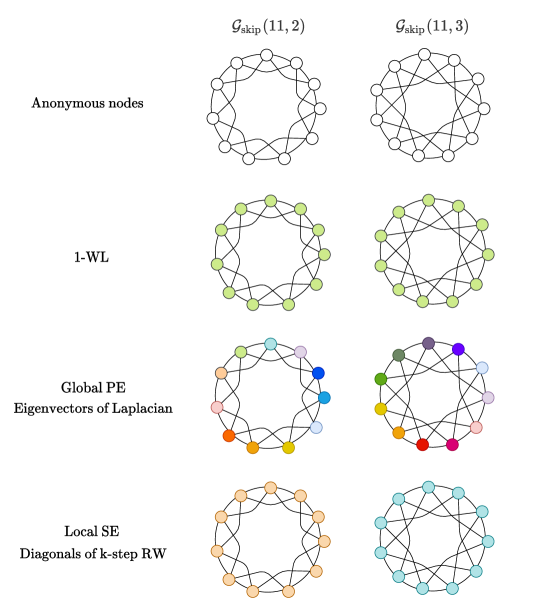
(a)

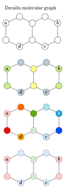
(b)

Figure C.1: First Row: Example graphs with anonymous nodes, i.e., nodes do not have any distinguishing node features. (a) A pair of Circular Skip Link (CSL) graphs [46] where the nodes have skip links of 2 and 3 respectively. (b) A Decalin molecular graph which has two rings of all Carbon atoms, thus with no distinguishing node features. Second Row: The nodes colored with the feature generated by 1-WL [59, 61, 45]. Third Row: The nodes colored with the feature generated by global PE [15]. Fourth Row: The nodes colored with the feature generated by local SE [16]. Note: The colors depicted on nodes in the graphs represent a unique feature vector generated, for a given graph, from the corresponding PE/SE. Figure best visualized in color.

The CSL graph, Figure 1(a).

In the CSL graph-pair [46], the two graphs $\mathcal{G}_{\textrm{\tiny skip}}(11,2)$ and $\mathcal{G}_{\textrm{\tiny skip}}(11,3)$ differ in the length of skip-link of a node and are hence non-isomorphic. Since the 1-WL algorithm produces the same color for all the nodes in both graphs, MPNNs will generate similar node colors. See the colors generated by 1-WL and MPNN in the second row of Figure 1(a). However, the use of a global PE (eg. Laplacian PE [15]) assigns each node a unique color, as depicted in the third row. Consequently, the feature embeddings of the two graphs which are the hash function outputs of the collection of node colors are different, thus making the task to distinguish the graphs successful. Similarly, the use of a local SE (e.g. diagonals of $m$-steps random walk) allows the coloring of the nodes of the 2 graphs to be different [16] since it captures the difference of the skip links of the two graphs successfully [42]. See the fourth row where the local SE based colors are depicted on the nodes. Therefore, either of the specific local SE or global PE can help distinguish the two graphs which cannot be learnt by 1-WL or MPNNs.

The Decalin molecular graph, Figure 1(b).

In the Decalin graph, the node $a$ is isomorphic to node $b$, and so is the node $c$ to node $d$. A 1-WL coloring of the nodes, and equivalently MPNN, would generate one color for the node $a,b$ and another color for $c,d$, see the second row in Figure 1(b). If that task is to identify a potential link between the node-sets $(a,d)$ and $(b,d)$, the combination of the node colors of the node-sets will produce the same embedding for the two links, thus making the 1-WL or MPNNs based coloring unsuitable to certain tasks [67]. A similar observation also follows for the node coloring based on the aforementioned local SE [16], which is illustrated in the fourth row in Figure 1(b). However, using a distance-based relative PE on the edges or an eigenvector-based global PE would successfully differentiate the embeddings of the two links. Therefore, the relative PE or the global PE which can help to distinguish between the two links cannot be learnt by 1-WL or MPNNs.

We can then conclude the following statement based on the above discussion which provides a theoretical basis for the need of PE and SE, as the PE and SE can be directly supplying essential information for the task:

Proposition 1. Assuming no modification applied to MPNNs for a learning task, there exists Positional Encodings (PE) and Structural Encoding (SE) which MPNNs are not guaranteed to learn.

C.2 Preserving edge information in the self-attention layer

In this section, we argue that an MPNN layer is able to propagate the information from edges to nodes such that, when computing the attention between nodes, the global Attention (Transformer) layer can infer whether two nodes are connected and what are the edge features between them.

Suppose an MPNN with the sum aggregator, with the update function as given below:

$$h_{u}^{l+1}=\sum_{v\in\mathcal{N}_{u}}{f(h_{u}^{l},h_{v}^{l},e_{uv})},$$ (5)

where $f$ is a learned function, e.g., an MLP; $u$ is the index of a central node whose neighborhood is being aggregated; $v$ is the index of a neighbor of $u$; $h^{l}_{u}$ the node features at layer $l$ for node $u$, and $e_{uv}$ the edge features between nodes $u$ and $v$.

We know from the Lemma 5 of Xu et al. [61] that the sum over a countable multiset is universal, meaning it can map a unique multiset to any possible function. Let’s assume that $h_{u}$ is unique and countable for every node $u$, which can be accomplised using all the Laplacian eigenvectors as PE. Then, there exist a function $f$ such that an encoding $\mu_{uv}$ that respects the following characteristics is propagated to the nodes: (i) unique for the triplet $\{h_{u},h_{v},e_{uv}\}$, (ii) invariant to the permutation of $u$ and $v$, (iii) contains the information of $e_{ij}$, (iv) all information of $\mu_{uv}$ is preserved after the $\sum$.

Hence, an Attention layer that follows the message-passing is able to infer whether two nodes are connected since both nodes will contain the unique identifier $\mu_{uv}$, and will also be able to infer the edge features from it.

An example of such function $\mu_{uv}$ is the tensor product $\otimes$ of a one-hot encoding unique for each edge $o_{uv}$ and the edge features $e_{uv}$. For example, if $e_{uv}=[e_{1},e_{2},e_{3}]$ and the edge is represented with $o_{uv}=[0,1,0,0]$, then $\mu_{uv}=o_{uv}\otimes e_{uv}=[0,0,0,e_{1},e_{2},e_{3},0,0,0,0,0,0]$ satisfies all the above conditions. Although this function requires an exponential increase in the hidden dimension, this is also the case for the Lemma 5 in Xu et al. [61].

Appendix D GPS schematics

D.1 GPS layer

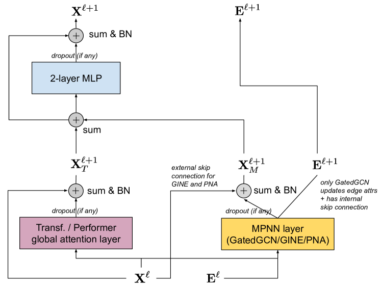
Figure D.1: Modular GPS layer that combines local MPNN and global attention blocks. Local MPNN encodes real edge features into the node-level hidden representations, while global attention mechanism can implicitly make use of this information together with PE/SE to infer relation between two nodes without explicit edge features. After each functional block (an MPNN layer, a global attention layer, an MLP) we apply residual connections followed by batch normalization (BN) [30]. In the 2-layer MLP block we use ReLU activations and its inner hidden dimension is twice the layer-input feature dimensionality $d_{\ell}$. Note, similarly to Transformer, the input and output dimensionality of the GPS-layer as a whole is the same.

GPS layer equations. In Section 3.3 of the main text we provide a simplify definition of the GPS computational layer for clarity, here we additionally list the precise application of skip connections, dropout, and batch normalization with learnable affine parameters:

$$\mathbf{X}^{\ell+1},\mathbf{E}^{\ell+1} = \texttt{GPS}^{\ell}\left(\mathbf{X}^{\ell},\mathbf{E}^{\ell},\mathbf{A}\right)$$ (6)

$$\textrm{computed as}\ \ \ \ \hat{\mathbf{X}}^{\ell+1}_{M},\ \mathbf{E}^{\ell+1} = \texttt{MPNN}_{e}^{\ell}\left(\mathbf{X}^{\ell},\mathbf{E}^{\ell},\mathbf{A}\right),$$ (7)

$$\hat{\mathbf{X}}^{\ell+1}_{T} = \texttt{GlobalAttn}^{\ell}\left(\mathbf{X}^{\ell}\right),$$ (8)

$$\mathbf{X}^{\ell+1}_{M} = \texttt{BatchNorm}\left(\texttt{Dropout}\left(\hat{\mathbf{X}}^{\ell+1}_{M}\right)+\mathbf{X}^{\ell}\right),$$ (9)

$$\mathbf{X}^{\ell+1}_{T} = \texttt{BatchNorm}\left(\texttt{Dropout}\left(\hat{\mathbf{X}}^{\ell+1}_{T}\right)+\mathbf{X}^{\ell}\right),$$ (10)

$$\mathbf{X}^{\ell+1} = \texttt{MLP}^{\ell}\left(\mathbf{X}^{\ell+1}_{M}+\mathbf{X}^{\ell+1}_{T}\right)$$ (11)

D.2 GPS algorithm

Algorithm 1 Algorithm for an $L$ layer GPS network.

Input: Graph $\mathcal{G}=(\mathcal{V},\mathcal{E})$ with $N$ nodes and $E$ edges; Adjacency matrix $\mathbf{A}\in\mathbb{R}^{N\times N}$; Node features $\mathbf{X}\in\mathbb{R}^{N\times D_{\textrm{\tiny node}}}$; Edge features $\mathbf{E}\in\mathbb{R}^{E\times D_{\textrm{\tiny edge}}}$; Local message passing model instance $\texttt{MPNN}_{e}$; Global attention model instance GlobalAttn; Positional Encoding function $F_{\textsc{pe}}$; Structural Encoding function $F_{\textsc{se}}$; Layer $\ell\in[0,L-1]$.
Output: Node representations $\mathbf{X}^{L}\in\mathbb{R}^{N\times D}$ and edge representations $\mathbf{E}^{L}\in\mathbb{R}^{E\times D}$, that can downstream be composed with appropriate prediction head for graph, node, or edge -level prediction.

1. $\mathbf{P}_{\textrm{\tiny node}},\mathbf{P}_{\textrm{\tiny edge}},\mathbf{S}_{\textrm{\tiny node}},\mathbf{S}_{\textrm{\tiny edge}}\ \leftarrow\ \emptyset$

2. if $F_{\textsc{pe}}$ is relative then $\mathbf{P}_{\textrm{\tiny edge}}\ \leftarrow F_{\textsc{pe}}(\mathcal{G})\ \in\mathbb{R}^{E\times D_{\textsc{pe}}}$  else  $\mathbf{P}_{\textrm{\tiny node}}\ \leftarrow F_{\textsc{pe}}(\mathcal{G})\ \in\mathbb{R}^{N\times D_{\textsc{pe}}}$

3. if $F_{\textsc{se}}$ is relative then $\mathbf{S}_{\textrm{\tiny edge}}\ \leftarrow F_{\textsc{se}}(\mathcal{G})\ \in\mathbb{R}^{E\times D_{\textsc{se}}}$  else  $\mathbf{S}_{\textrm{\tiny node}}\ \leftarrow F_{\textsc{se}}(\mathcal{G})\ \in\mathbb{R}^{N\times D_{\textsc{se}}}$

4. $\mathbf{X}^{0}\ \leftarrow\ \bigoplus_{\textrm{\tiny node}}\bigl{(}\texttt{NodeEncoder}\left(\mathbf{X}\right),\mathbf{P}_{\textrm{\tiny node}},\mathbf{S}_{\textrm{\tiny node}}\bigr{)}\ \in\mathbb{R}^{N\times D}$

5. $\mathbf{E}^{0}\ \leftarrow\ \bigoplus_{\textrm{\tiny edge}}\bigl{(}\texttt{EdgeEncoder}\left(\mathbf{E}\right),\mathbf{P}_{\textrm{\tiny edge}},\mathbf{S}_{\textrm{\tiny edge}}\bigr{)}\ \in\mathbb{R}^{E\times D}$

6. for $\ell=0,1,\cdots,L-1$

   1. $\hat{\mathbf{X}}^{\ell+1}_{M},\ \mathbf{E}^{\ell+1}\leftarrow\texttt{MPNN}_{e}^{\ell}\left(\mathbf{X}^{\ell},\mathbf{E}^{\ell},\mathbf{A}\right)$

   2. $\hat{\mathbf{X}}^{\ell+1}_{T}\leftarrow\texttt{GlobalAttn}^{\ell}\left(\mathbf{X}^{\ell}\right)$

   3. $\mathbf{X}^{\ell+1}_{M}\leftarrow\texttt{BatchNorm}\left(\texttt{Dropout}\left(\hat{\mathbf{X}}^{\ell+1}_{M}\right)+\mathbf{X}^{\ell}\right)$

   4. $\mathbf{X}^{\ell+1}_{T}\leftarrow\texttt{BatchNorm}\left(\texttt{Dropout}\left(\hat{\mathbf{X}}^{\ell+1}_{T}\right)+\mathbf{X}^{\ell}\right)$

   5. $\mathbf{X}^{\ell+1}\leftarrow\texttt{MLP}^{\ell}\left(\mathbf{X}^{\ell+1}_{M}+\mathbf{X}^{\ell+1}_{T}\right)$

7. return $\mathbf{X}^{L}\in\mathbb{R}^{N\times D}$ and $\mathbf{E}^{L}\in\mathbb{R}^{E\times D}$

where $\bigoplus$ denotes an operator for combining the input node or edge features with their respective positional and/or structural encoding, in practice this is a concatenation operator which can be changed to sum or other operators; NodeEncoder and EdgeEncoder are dataset-specific initial node and edge feature encoders potentially with learnable parameters; $\texttt{MPNN}_{e}$ and GlobalAttn have their corresponding learnable parameters at each layer $\ell$; $\hat{\mathbf{X}}^{\ell+1}_{M}$ and $\hat{\mathbf{X}}^{\ell+1}_{T}$ denote the intermediate node representations given by the local message passing module and the global attention module respectively; and $\texttt{MLP}^{\ell}$ is a multi layer perceptron module with its own learnable parameters that combines the intermediate $\mathbf{X}^{\ell+1}_{M}$ and $\mathbf{X}^{\ell+1}_{T}$. Note that a relative $F_{\textsc{pe}}$ or $F_{\textsc{se}}$ produces PE or SE for each edge which are thence handled accordingly in lines 2 and 3 in Algorithm 1.

References

- Alon and Yahav [2021] Uri Alon and Eran Yahav. On the bottleneck of graph neural networks and its practical implications. In International Conference on Learning Representations, 2021.
- Andres et al. [2016] Sebastian Andres, Jean-Dominique Deuschel, and Martin Slowik. Heat kernel estimates for random walks with degenerate weights. Electronic Journal of Probability, 21:1–21, 2016.
- Beaini et al. [2021] Dominique Beaini, Saro Passaro, Vincent Létourneau, Will Hamilton, Gabriele Corso, and Pietro Liò. Directional graph networks. In International Conference on Machine Learning, pages 748–758. PMLR, 2021.
- Beltagy et al. [2020] Iz Beltagy, Matthew E. Peters, and Arman Cohan. Longformer: The long-document transformer. CoRR, abs/2004.05150, 2020.
- Bodnar et al. [2021] Cristian Bodnar, Fabrizio Frasca, Nina Otter, Yuguang Wang, Pietro Lio, Guido F Montufar, and Michael Bronstein. Weisfeiler and Lehman go cellular: CW networks. Advances in Neural Information Processing Systems, 34:2625–2640, 2021.
- Bouritsas et al. [2022] Giorgos Bouritsas, Fabrizio Frasca, Stefanos P Zafeiriou, and Michael Bronstein. Improving graph neural network expressivity via subgraph isomorphism counting. IEEE Transactions on Pattern Analysis and Machine Intelligence, 2022.
- Bresson and Laurent [2017] Xavier Bresson and Thomas Laurent. Residual Gated Graph ConvNets. arXiv:1711.07553, 2017.
- Chelombiev et al. [2021] Ivan Chelombiev, Daniel Justus, Douglas Orr, Anastasia Dietrich, Frithjof Gressmann, Alexandros Koliousis, and Carlo Luschi. Groupbert: Enhanced transformer architecture with efficient grouped structures. arXiv:2106.05822, 2021.
- Chen et al. [2022] Dexiong Chen, Leslie O’Bray, and Karsten Borgwardt. Structure-aware transformer for graph representation learning. Proceedings of the 39th International Conference on Machine Learning, 2022.
- Chen et al. [2019] Zhengdao Chen, Lei Chen, Soledad Villar, and Joan Bruna. On the equivalence between graph isomorphism testing and function approximation with gnns. Advances in Neural Information Processing Systems, 2019.
- Choromanski et al. [2021a] Krzysztof Choromanski, Han Lin, Haoxian Chen, Tianyi Zhang, Arijit Sehanobish, Valerii Likhosherstov, Jack Parker-Holder, Tamas Sarlos, Adrian Weller, and Thomas Weingarten. From block-Toeplitz matrices to differential equations on graphs: towards a general theory for scalable masked transformers. arXiv:2107.07999, 2021a.
- Choromanski et al. [2021b] Krzysztof Marcin Choromanski, Valerii Likhosherstov, David Dohan, Xingyou Song, Andreea Gane, Tamás Sarlós, Peter Hawkins, Jared Quincy Davis, Afroz Mohiuddin, Lukasz Kaiser, David Benjamin Belanger, Lucy J. Colwell, and Adrian Weller. Rethinking attention with performers. In 9th International Conference on Learning Representations, 2021b.
- Corso et al. [2020] Gabriele Corso, Luca Cavalleri, Dominique Beaini, Pietro Liò, and Petar Veličković. Principal neighbourhood aggregation for graph nets. Advances in Neural Information Processing Systems, 33:13260–13271, 2020.
- Dwivedi and Bresson [2020] Vijay Prakash Dwivedi and Xavier Bresson. A generalization of transformer networks to graphs. arXiv:2012.09699, 2020.
- Dwivedi et al. [2020] Vijay Prakash Dwivedi, Chaitanya K Joshi, Thomas Laurent, Yoshua Bengio, and Xavier Bresson. Benchmarking graph neural networks. arXiv:2003.00982, 2020.
- Dwivedi et al. [2022a] Vijay Prakash Dwivedi, Anh Tuan Luu, Thomas Laurent, Yoshua Bengio, and Xavier Bresson. Graph neural networks with learnable structural and positional representations. In International Conference on Learning Representations, 2022a.
- Dwivedi et al. [2022b] Vijay Prakash Dwivedi, Ladislav Rampášek, Mikhail Galkin, Ali Parviz, Guy Wolf, Anh Tuan Luu, and Dominique Beaini. Long range graph benchmark. Neural Information Processing Systems (NeurIPS 2022), Track on Datasets and Benchmarks, 2022b.
- d’Ascoli et al. [2021] Stéphane d’Ascoli, Hugo Touvron, Matthew L Leavitt, Ari S Morcos, Giulio Biroli, and Levent Sagun. Convit: Improving vision transformers with soft convolutional inductive biases. In International Conference on Machine Learning, pages 2286–2296. PMLR, 2021.
- Ertl and Schuffenhauer [2009] Peter Ertl and Ansgar Schuffenhauer. Estimation of synthetic accessibility score of drug-like molecules based on molecular complexity and fragment contributions. Journal of cheminformatics, 1(1):1–11, 2009.
- Fey and Lenssen [2019] Matthias Fey and Jan Eric Lenssen. Fast graph representation learning with PyTorch Geometric. In ICLR Workshop on Representation Learning on Graphs and Manifolds, 2019.
- Freitas et al. [2021] Scott Freitas, Yuxiao Dong, Joshua Neil, and Duen Horng Chau. A large-scale database for graph representation learning. In 35th Conference on Neural Information Processing Systems: Datasets and Benchmarks Track, 2021.
- Gilmer et al. [2017] Justin Gilmer, Samuel S Schoenholz, Patrick F Riley, Oriol Vinyals, and George E Dahl. Neural message passing for quantum chemistry. In International conference on machine learning, pages 1263–1272. PMLR, 2017.
- Gu et al. [2022] Albert Gu, Karan Goel, and Christopher Re. Efficiently modeling long sequences with structured state spaces. In International Conference on Learning Representations, 2022.
- Guo et al. [2021] Jianyuan Guo, Kai Han, Han Wu, Chang Xu, Yehui Tang, Chunjing Xu, and Yunhe Wang. CMT: Convolutional neural networks meet vision transformers. arXiv:2107.06263, 2021.
- Han et al. [2022] Kai Han, Yunhe Wang, Hanting Chen, Xinghao Chen, Jianyuan Guo, Zhenhua Liu, Yehui Tang, An Xiao, Chunjing Xu, Yixing Xu, et al. A survey on vision transformer. IEEE Transactions on Pattern Analysis and Machine Intelligence, 2022.
- Hu et al. [2019] Weihua Hu, Bowen Liu, Joseph Gomes, Marinka Zitnik, Percy Liang, Vijay Pande, and Jure Leskovec. Strategies for pre-training graph neural networks. arXiv:1905.12265, 2019.
- Hu et al. [2020] Weihua Hu, Matthias Fey, Marinka Zitnik, Yuxiao Dong, Hongyu Ren, Bowen Liu, Michele Catasta, and Jure Leskovec. Open Graph Benchmark: Datasets for Machine Learning on Graphs. 34th Conference on Neural Information Processing Systems, 2020.
- Hu et al. [2021] Weihua Hu, Matthias Fey, Hongyu Ren, Maho Nakata, Yuxiao Dong, and Jure Leskovec. OGB-LSC: A large-scale challenge for machine learning on graphs. In 35th Conference on Neural Information Processing Systems: Datasets and Benchmarks Track, 2021.
- Hussain et al. [2022] Md Shamim Hussain, Mohammed J Zaki, and Dharmashankar Subramanian. Global self-attention as a replacement for graph convolution. In Proceedings of the 28th ACM SIGKDD Conference on Knowledge Discovery and Data Mining, pages 655–665, 2022.
- Ioffe and Szegedy [2015] Sergey Ioffe and Christian Szegedy. Batch normalization: Accelerating deep network training by reducing internal covariate shift. In International conference on machine learning, pages 448–456. PMLR, 2015.
- Jain et al. [2021] Paras Jain, Zhanghao Wu, Matthew Wright, Azalia Mirhoseini, Joseph E Gonzalez, and Ion Stoica. Representing long-range context for graph neural networks with global attention. Advances in Neural Information Processing Systems, 34, 2021.
- Kalyan et al. [2021] Katikapalli Subramanyam Kalyan, Ajit Rajasekharan, and Sivanesan Sangeetha. Ammus: A survey of transformer-based pretrained models in natural language processing. arXiv:2108.05542, 2021.
- Kipf and Welling [2016] Thomas N Kipf and Max Welling. Semi-supervised classification with graph convolutional networks. arXiv:1609.02907, 2016.
- Kitaev et al. [2020] Nikita Kitaev, Lukasz Kaiser, and Anselm Levskaya. Reformer: The efficient transformer. In 8th International Conference on Learning Representations, 2020.
- Koutis and Le [2019] Ioannis Koutis and Huong Le. Spectral modification of graphs for improved spectral clustering. Advances in Neural Information Processing Systems, 32, 2019.
- Kreuzer et al. [2021] Devin Kreuzer, Dominique Beaini, William L. Hamilton, Vincent Létourneau, and Prudencio Tossou. Rethinking graph transformers with spectral attention. In Advances in Neural Information Processing Systems, 2021.
- Kurin et al. [2020] Vitaly Kurin, Maximilian Igl, Tim Rocktäschel, Wendelin Boehmer, and Shimon Whiteson. My body is a cage: the role of morphology in graph-based incompatible control. arXiv:2010.01856, 2020.
- Li et al. [2020] Pan Li, Yanbang Wang, Hongwei Wang, and Jure Leskovec. Distance encoding: Design provably more powerful neural networks for graph representation learning. Advances in Neural Information Processing Systems, 33:4465–4478, 2020.
- Lim et al. [2022] Derek Lim, Joshua Robinson, Lingxiao Zhao, Tess Smidt, Suvrit Sra, Haggai Maron, and Stefanie Jegelka. Sign and basis invariant networks for spectral graph representation learning. arXiv:2202.13013, 2022.
- Liu et al. [2022] Shizhan Liu, Hang Yu, Cong Liao, Jianguo Li, Weiyao Lin, Alex X. Liu, and Schahram Dustdar. Pyraformer: Low-complexity pyramidal attention for long-range time series modeling and forecasting. In International Conference on Learning Representations, 2022.
- Loshchilov and Hutter [2019] Ilya Loshchilov and Frank Hutter. Decoupled weight decay regularization. In International Conference on Learning Representations, 2019.
- Loukas [2020] Andreas Loukas. What graph neural networks cannot learn: depth vs width. In International Conference on Learning Representations, 2020.
- Maron et al. [2019] Haggai Maron, Heli Ben-Hamu, Hadar Serviansky, and Yaron Lipman. Provably powerful graph networks. arXiv:1905.11136, 2019.
- Mialon et al. [2021] Grégoire Mialon, Dexiong Chen, Margot Selosse, and Julien Mairal. GraphiT: Encoding graph structure in transformers. arXiv:2106.05667, 2021.
- Morris et al. [2019] Christopher Morris, Martin Ritzert, Matthias Fey, William L. Hamilton, Jan Eric Lenssen, Gaurav Rattan, and Martin Grohe. Weisfeiler and Leman go neural: Higher-order graph neural networks. In The Thirty-Third AAAI Conference on Artificial Intelligence, pages 4602–4609. AAAI Press, 2019.
- Murphy et al. [2019] Ryan Murphy, Balasubramaniam Srinivasan, Vinayak Rao, and Bruno Ribeiro. Relational pooling for graph representations. In International Conference on Machine Learning, pages 4663–4673. PMLR, 2019.
- Oono and Suzuki [2020] Kenta Oono and Taiji Suzuki. Graph neural networks exponentially lose expressive power for node classification. In International Conference on Learning Representations, 2020.
- Park et al. [2022] Wonpyo Park, Woonggi Chang, Donggeon Lee, Juntae Kim, and Seung won Hwang. GRPE: Relative positional encoding for graph transformer. arXiv:22201.12787, 2022.
- Raffel et al. [2020] Colin Raffel, Noam Shazeer, Adam Roberts, Katherine Lee, Sharan Narang, Michael Matena, Yanqi Zhou, Wei Li, and Peter J. Liu. Exploring the limits of transfer learning with a unified text-to-text transformer. Journal of Machine Learning Research, 21(140):1–67, 2020.
- Sato [2020] Ryoma Sato. A survey on the expressive power of graph neural networks. arXiv:2003.04078, 2020.
- Shi et al. [2022] Yu Shi, Shuxin Zheng, Guolin Ke, Yifei Shen, Jiacheng You, Jiyan He, Shengjie Luo, Chang Liu, Di He, and Tie-Yan Liu. Benchmarking graphormer on large-scale molecular modeling datasets. arXiv:2203.04810, 2022.
- Tay et al. [2021] Yi Tay, Mostafa Dehghani, Samira Abnar, Yikang Shen, Dara Bahri, Philip Pham, Jinfeng Rao, Liu Yang, Sebastian Ruder, and Donald Metzler. Long range arena: A benchmark for efficient transformers. In International Conference on Learning Representations, 2021.
- Toenshoff et al. [2021] Jan Toenshoff, Martin Ritzert, Hinrikus Wolf, and Martin Grohe. Graph learning with 1d convolutions on random walks. arXiv:2102.08786, 2021.
- Topping et al. [2021] Jake Topping, Francesco Di Giovanni, Benjamin Paul Chamberlain, Xiaowen Dong, and Michael M Bronstein. Understanding over-squashing and bottlenecks on graphs via curvature. arXiv:2111.14522, 2021.
- Vaswani et al. [2017] Ashish Vaswani, Noam Shazeer, Niki Parmar, Jakob Uszkoreit, Llion Jones, Aidan N Gomez, Łukasz Kaiser, and Illia Polosukhin. Attention is all you need. Advances in Neural Information Processing Systems, 30, 2017.
- Veličković et al. [2018] Petar Veličković, Guillem Cucurull, Arantxa Casanova, Adriana Romero, Pietro Liò, and Yoshua Bengio. Graph attention networks. In International Conference on Learning Representations, 2018.
- Wang et al. [2022] Haorui Wang, Haoteng Yin, Muhan Zhang, and Pan Li. Equivariant and stable positional encoding for more powerful graph neural networks. In International Conference on Learning Representations, 2022.
- Wang et al. [2020] Sinong Wang, Belinda Z. Li, Madian Khabsa, Han Fang, and Hao Ma. Linformer: Self-attention with linear complexity. arXiv:2006.04768, 2020.
- Weisfeiler and Leman [1968] Boris Weisfeiler and Andrei Leman. The reduction of a graph to canonical form and the algebra which appears therein. NTI, Series, 2(9):12–16, 1968.
- Wildman and Crippen [1999] Scott A Wildman and Gordon M Crippen. Prediction of physicochemical parameters by atomic contributions. Journal of chemical information and computer sciences, 39(5):868–873, 1999.
- Xu et al. [2019] Keyulu Xu, Weihua Hu, Jure Leskovec, and Stefanie Jegelka. How powerful are graph neural networks? In International Conference on Learning Representations, 2019.
- Yang et al. [2022] Mingqi Yang, Renjian Wang, Yanming Shen, Heng Qi, and Baocai Yin. Breaking the expression bottleneck of graph neural networks. IEEE Transactions on Knowledge and Data Engineering, 2022.
- Ying et al. [2021a] Chengxuan Ying, Tianle Cai, Shengjie Luo, Shuxin Zheng, Guolin Ke, Di He, Yanming Shen, and Tie-Yan Liu. Do transformers really perform badly for graph representation? In Advances in Neural Information Processing Systems, 2021a.
- Ying et al. [2021b] Chengxuan Ying, Mingqi Yang, Shuxin Zheng, Guolin Ke, Shengjie Luo, Tianle Cai, Chenglin Wu, Yuxin Wang, Yanming Shen, and Di He. First place solution of KDD Cup 2021 & OGB large-scale challenge graph prediction track. arXiv:2106.08279, 2021b.
- You et al. [2020] Jiaxuan You, Rex Ying, and Jure Leskovec. Design space for graph neural networks. In Advances in Neural Information Processing Systems, 2020.
- Zaheer et al. [2020] Manzil Zaheer, Guru Guruganesh, Kumar Avinava Dubey, Joshua Ainslie, Chris Alberti, Santiago Ontañón, Philip Pham, Anirudh Ravula, Qifan Wang, Li Yang, and Amr Ahmed. Big Bird: Transformers for longer sequences. In Advances in Neural Information Processing Systems, 2020.
- Zhang et al. [2021] Muhan Zhang, Pan Li, Yinglong Xia, Kai Wang, and Long Jin. Labeling trick: A theory of using graph neural networks for multi-node representation learning. Advances in Neural Information Processing Systems, 34, 2021.
- Zhao et al. [2022] Lingxiao Zhao, Wei Jin, Leman Akoglu, and Neil Shah. From stars to subgraphs: Uplifting any GNN with local structure awareness. In International Conference on Learning Representations, 2022.