Detecting Abrupt Changes in Sequential Pairwise Comparison Data

Abstract

The Bradley-Terry-Luce (BTL) model is a classic and very popular statistical approach for eliciting a global ranking among a collection of items using pairwise comparison data. In applications in which the comparison outcomes are observed as a time series, it is often the case that data are non-stationary, in the sense that the true underlying ranking changes over time. In this paper we are concerned with localizing the change points in a high-dimensional BTL model with piece-wise constant parameters. We propose novel and practicable algorithms based on dynamic programming that can consistently estimate the unknown locations of the change points. We provide consistency rates for our methodology that depend explicitly on the model parameters, the temporal spacing between two consecutive change points and the magnitude of the change. We corroborate our findings with extensive numerical experiments and a real-life example.

1 Introduction

Pairwise comparison data are among the most common types of data collected for the purpose of eliciting a global ranking among a collection of items or teams. The Bradley-Terry-Luce model (Bradley and Terry,, 1952; Luce,, 1959) is a classical and popular parametric approach to model pairwise comparison data and to obtain an estimate of the underlying ranking. The Bradley-Terry-Luce model and its variants have been proven to be powerful approaches in many applications, including sports analytics (Fahrmeir and Tutz,, 1994; Masarotto and Varin,, 2012; Cattelan et al.,, 2013), bibliometrics (Stigler,, 1994; Varin et al.,, 2016), search analytics (Radlinski and Joachims,, 2007; Agresti,, 2013), and much more.

To introduce the BTL model, suppose that we are interested in ranking $n$ distinct items, each with a (fixed but unobserved) positive preference score $w_{i}$, $i\in[n]$, quantifying its propensity to beat other items in a pairwise comparison. The BTL model assumes that the outcomes of the comparisons between different pairs are independent Bernoulli random variables such that, for a given pair of items, say $i$ and $j$ in $[n]:=\{1,\ldots,n\}$, the probability that $i$ is preferred to (or beats) $j$ is

$$P_{ij}=\mathbb{P}\left(i\text{ beats }j\right)=\frac{w^{*}_{i}}{w^{*}_{i}+w^{*}_{j}},\>\forall\;i,j\in[n].$$ (1.1)

A common reparametrization is to set $w^{*}_{i}=\exp(\theta^{*}_{i})$ for each $i$, where $\bm{\theta}^{*}:=(\theta^{*}_{1},\ldots,\theta^{*}_{n})^{\top}\in\mathbb{R}^{n}$. To ensure identifiability it is further assumed that $\sum_{i\in[n]}\theta^{*}_{i}=0$.

The properties and performance of the BTL model have been thoroughly studied under the assumption that the outcomes of all the pairwise comparisons are simultaneously available and follow the same BTL model. In many applications however, it is very common to observe pairwise comparison data sequentially (i.e. one at a time), with time stamps over multiple time periods. In these cases, it is unrealistic to assume that observations with different time stamps come from the same distribution. For instance, in sports analytics, the performance of teams often changes across match rounds, and Fahrmeir and Tutz, (1994) utilized a state-space generalization of the BTL model to analyze sport tournaments data. Ranking analysis with temporal variants has also become increasingly important because of the growing needs for models and methods to handle time-dependent data. A series of results in this direction can be found in Glickman, (1993), Glickman and Stern, (1998), Cattelan et al., (2013), Lopez et al., (2018), Maystre et al., (2019), Bong et al., (2020), Karlé and Tyagi, (2021) and references therein. Much of the aforementioned literature on time-varying BTL model postulates that temporal changes in the model parameters are smooth functions of time and thus occur gradually on a relatively large time scale. However, there are instances in which it may be desirable to instead model abrupt changes in the underlying parameters and estimate the times at which such change has occurred. These change point settings, which, to the best of our knowledge, have not been considered in the literature, and are the focus of this paper.

Contributions

We make the following methodological and theoretical contributions.

$\bullet$ Novel change point methodology. We develop a computationally efficient methodology to consistently estimate the change points for a time-varying BTL model with piece-wise constant parameters. Our baseline procedure Algorithm 1 consists of a penalized maximum likelihood estimator of the BTL model under an $\ell_{0}$ penalty, and can be efficiently implemented via dynamic programming. We further propose a slightly more computationally expensive two-step procedure in Algorithm 2 that takes as input the estimator returned by our baseline procedure and delivers a more precise estimator with provably better error rates. We demonstrate through simulations and a real life example the performance and practicality of the procedure we develop.

$\bullet$ Theoretical guarantees. We obtain finite sample error rates for our procedures that depend explicitly on all the parameters at play: the dynamic range of the BTL model and the number of items to be compared, the number of change points, the smallest distance between two consecutive change points and the minimal magnitude of the difference between the model parameters at two consecutive change points. Importantly, our theory allows for general connected comparison graph and it explicitly captures the effect the topology of the comparison graph. Our results hold provided that a critical signal-to-noise ratio condition involving all the relevant parameters is satisfied. We conjecture that this condition is optimal in an information theoretic sense. Both the signal-to-noise ratio condition and the localization rates we obtain exhibit a quadratic dependence on the number of items to be compared, which matches the sample complexity bound for two sample testing for the BTL model recently derived by Rastogi et al., (2020).

We emphasize that the change point setting we consider have not been previously studied and both our methodology and the corresponding theoretical guarantees appear to be the first contribution of its kind in this line of work.

Related work

Change point detection is a classical problem in statistics that dates back to 1940s (Wald,, 1945; Page,, 1954). Contributions in the 1980s established asymptotic theory for change point detection methods (Vostrikova,, 1981; James et al.,, 1987; Yao and Au,, 1989). Most of the classical literature studied the univariate mean model. Recently with more advanced theoretical tools developed in modern statistics, more delicate analysis of change point detection came out in high-dimensional mean models (Jirak,, 2015; Aston and Kirch,, 2018; Wang and Samworth,, 2018), covariance models (Aue et al.,, 2009; Avanesov and Buzun,, 2018; Wang et al., 2021b, ), high-dimensional regression models (Rinaldo et al.,, 2021; Wang et al., 2021c, ), network models (Wang et al., 2021a, ), and temporally-correlated times series (Cho and Fryzlewicz,, 2015; Preuss et al.,, 2015; Chen et al.,, 2021; Wang and Zhao,, 2022).

Although change point detection has already been extensively studied in many different settings, little is known about the case of pairwise comparison data. Höhle, (2010) numerically study the CUSUM method for online change point detection in logit models and BTL models without giving theoretical guarantees. We aim to fill the gap in the literature and propose a theoretically trackable approach that can optimally localize abrupt changes in the pairwise comparison data.

2 Model and assumptions

Below we introduce the time-varying BTL model with piece-wise constant coefficients that we are going to study and the sampling scheme for collecting pairwise comparison data over time.

Suppose there is a connected comparison graph $\mathcal{G}=\mathcal{G}([n],E)$ with edge set $E\subseteq E_{\rm full}:=\{(i,j):1\leq i<j\leq n\}$. We assume throughout that data are collected as a time series indexed by $t\in[T]:=\{1,\ldots,T\}$ that, at each time point $t$, a single pairwise comparison among a collection of $n$ items is observed. The distinct pair $(i_{t},j_{t})\in[n]^{2}$ of items to be compared at time $t$ is randomly chosen from the edge set $E$ of $\mathcal{G}$, independently over time. That is,

$$\mathbb{P}(i_{t}=i,j_{t}=j)=\frac{1}{|E|},\ \forall(i,j)\in E.$$ (2.1)

For each $t$, let $y_{t}\in\{0,1\}$ denote the outcome of the comparison between $i_{t}$ and $j_{t}$, where $y_{t}=1$ indicates that $i_{t}$ beats $j_{t}$ in the comparison. We assume that $y_{t}$ follows the BTL model (1.1), i.e.

$$\mathbb{P}_{\bm{\theta}^{*}(t)}[y_{t}=1|(i_{t},j_{t})]=\frac{e^{\theta^{*}_{i_{t}}(t)}}{e^{\theta^{*}_{i_{t}}(t)}+e^{\theta^{*}_{j_{t}}(t)}},$$ (2.2)

where $\bm{\theta}^{*}(t)=(\theta^{*}_{1}(t),\ldots\theta^{*}_{n}(t))$ is, a possibly time-varying, parameter that belongs to the set

$$\Theta_{B}:=\{\bm{\theta}\in\mathbb{R}^{n}:\mathbf{1}_{n}^{\top}\bm{\theta}=0,\ \|\bm{\theta}\|_{\infty}\leq B\},$$ (2.3)

for some $B>0$. In the recent literature on the BTL model, the parameter $B$ is referred to as the dynamic range (see, e.g., Chen et al.,, 2019) which readily implies a bound on the smallest possible probability that an item is beaten by any other item. Indeed, it follows from (2.2) and (2.3) that

$$\min_{t\in[T],i,j\in[n]}P_{ij}(t)\geq e^{-2B}/(1+e^{-2B}):=p_{lb}>0.$$ (2.4)

Remark 1.

The quantity $p_{lb}$ have appeared in several equivalent forms in the BTL literature, e.g., $\max_{i,j\in[n]}\frac{w^{*}_{i}}{w^{*}_{j}}$ (Simons and Yao,, 1999; Negahban et al.,, 2017) and $e^{2B}$ (Li et al.,, 2022). The minimal winning probability $p_{lb}$ provides a way of quantifying the difficulty in estimating the model parameters, with a small $p_{lb}$ implying that some items are systematically better than others, a fact that is known to lead to non-existence of the MLE (see, e.g. Ford,, 1957) and to hinder parameter estimability. In the BTL literature the dynamic range $B$ and, as a result, the quantity $p_{lb}$ are often treated as known constants and thus omitted (Shah et al.,, 2016; Chen et al.,, 2020), a strong assumption that results in an implicit regularization but potentially hides an important feature of the model. As argued in Bong and Rinaldo, (2022), in high-dimensional settings this may not be realistic. We will allow for the possibility of a varying $B$ and $p_{lb}$, and keep track of the effect of these parameters on our consistency rates.

It is convenient to rewrite (2.2) in a different but equivalent form that is reminiscent of logistic regression and will facilitate our analysis. One can express the fact that, at time $t$, the items $i_{t}$ and $j_{t}$ are randomly selected from $\mathcal{G}([n],E)$ to be compared using a random $n$-dimensional vector $\mathbf{x}(t)$ that is drawn from the sets of all vectors in $\{-1,0,1\}^{n}$ with exactly two-non-zero entries of opposite sign, namely $x_{i_{t}}(t)=1$ and $x_{j_{t}}(t)=-1$ for $(i_{t},j_{t})\in E$. Then equation (2.2) can be written as

$$\mathbb{P}_{\bm{\theta}^{*}(t)}[y_{t}=1|\mathbf{x}(t)]=\psi\left({\mathbf{x}(t)^{\top}\bm{\theta}^{*}(t)}\right),$$ (2.5)

where $\psi(x)=\frac{1}{1+e^{-x}}$ is the sigmoid function. For any time interval $\mathcal{I}\subset[T]$ we then assume that the data take the form of an i.i.d. sequence $\{(\mathbf{x}(t),y_{t})\}_{t\in\mathcal{I}}$, where each $\mathbf{x}(t)$ is an i.i.d. draw from $\{-1,0,1\}^{n}$ with aforementioned properties and, conditionally on $\mathbf{x}(t)$, $y_{t}$ is a Bernoulli random variable with success probability (2.2). The negative log-likelihood of the data is then given by

$$L({\bm{\theta}},\mathcal{I})=\sum_{t\in\mathcal{I}}\ell_{t}(\bm{\theta}),\ \text{where}\ \ell_{t}(\bm{\theta}):=\ell(\bm{\theta};y_{t},\mathbf{x}(t))=-y_{t}\mathbf{x}(t)^{\top}{\bm{\theta}}+\log[1+\exp(\mathbf{x}(t)^{\top}{\bm{\theta}})].$$ (2.6)

For a time interval $\mathcal{I}$, we can define a random comparison graph $\mathcal{G}_{\mathcal{I}}(V_{\mathcal{I}},E_{\mathcal{I}})$ with vertex set $V:=[n]$ and edge set $E_{\mathcal{I}}:=\{(i,j):i\text{ and }j\text{ are compared in }\mathcal{I}\}$. It is well-known that the topology of $\mathcal{G}_{\mathcal{I}}(V_{\mathcal{I}},E_{\mathcal{I}})$ plays an important role in the estimation of BTL parameters (Shah et al.,, 2016). Under assumption (2.1), the comparison graph over $\mathcal{I}$ follows the random graph model $G([n],|\mathcal{I}|)$, which has $|\mathcal{I}|$ edges randomly picked from the edge set $E$ with replacement. Therefore, the process $\{(\mathbf{x}(t),y_{t})\}_{t\in\mathcal{I}}$ is stationary as long as $\bm{\theta}^{*}(t)$ is unchanged over $\mathcal{I}$.

In the change point BTL model we assume that, for some unknown integer $K\geq 1$, there exist $K+2$ points $\{\eta_{k}\}_{k=0}^{K+1}$ such that $1=\eta_{0}<\eta_{1}<\cdots<\eta_{K}<\eta_{K+1}=T$ and $\bm{\theta}^{*}(t)\neq\bm{\theta}^{*}(t-1)$ whenever $t\in\{\eta_{k}\}_{k\in[K]}$. Define the minimal spacing $\Delta$ between consecutive change points and the minimal jump size $\kappa$ as

$$\Delta=\min_{k\in[K+1]}(\eta_{k}-\eta_{k-1}),\quad\kappa=\min_{k\in[K+1]}\|\bm{\theta}^{*}(\eta_{k})-\bm{\theta}^{*}(\eta_{k-1})\|_{2}.$$ (2.7)

As we mentioned in the introduction, the goal of change point localization is to produce an estimator of the change points $\{\hat{\eta}_{k}\}_{k\in[\hat{K}]}$ such that, with high-probability as $T\rightarrow\infty$, we recover the correct number of change points and the localization error is a vanishing fraction of the minimal distance between change points, i.e. that

$$\hat{K}=K,\text{ and }\max_{k\in[K]}|\hat{\eta}_{k}-\eta_{k}|/\Delta=o(1).$$ (2.8)

In change point literature, estimators satisfying the above conditions are called consistent. In the next section we will present two change point estimators and prove their consistency.

3 Main results

To estimate the change points, we solve the following regularized maximum likelihood problem over all possible partitions $\mathcal{P}$ of the time course $[T]$:

$$\hat{\mathcal{P}}=\operatornamewithlimits{arg\,min}_{\mathcal{P}}\left\{\sum_{\mathcal{I}\in\mathcal{P}}L(\hat{\bm{\theta}}(\mathcal{I}),\mathcal{I})+\gamma|\mathcal{P}|\right\},\quad\hat{\bm{\theta}}(\mathcal{I})=\operatornamewithlimits{arg\,min}_{\bm{\theta}\in\Theta_{B}}L(\bm{\theta},\mathcal{I}),$$ (3.1)

where $L(\bm{\theta},\mathcal{I})$ is the negative log-likelihood function for the BTL model defined in (2.6) and $\gamma>0$ is an user-specified tuning parameter. Here a partition $\mathcal{P}$ is defined as a set of integer intervals:

$$\mathcal{P}=\{[1,p_{1}),[p_{1},p_{2}),\ldots,[p_{K_{\mathcal{P}}},T]\},1<p_{1}<p_{2}<\cdots<p_{K_{\mathcal{P}}}<T.$$ (3.2)

With $\tilde{K}=K_{\hat{\mathcal{P}}}=|\hat{\mathcal{P}}|-1$, the estimated change points $\{\tilde{\eta}_{k}\}_{k\in\tilde{K}}$ are then induced by $\tilde{\eta}_{k}=\hat{p}_{k}$, $k\in[\tilde{K}]$. The optimization problem (3.1) has an $\ell_{0}$-penalty, and can be solved by a dynamic programming algorithm described in Algorithm 1 with $O(T^{2}\mathcal{C}(T))$ complexity (Friedrich et al.,, 2008; Rinaldo et al.,, 2021), where $\mathcal{C}(T)$ is the complexity of solving $\min_{\bm{\theta}}L(\bm{\theta},[1,T])$.

In this section, we will demonstrate that the estimator returned by Algorithm 1 is consistent. Towards that goal, we require the following signal-to-noise ratio condition involving the parameters $\Delta$, $\kappa$, $B$, $n$, the sample size $T$, and the topological property of the underlying comparison graph $\mathcal{G}([n],E)$.

Assumption 3.1 (Signal-to-noise ratio).

Let $\{(\mathbf{x}(t),y_{t})\}_{t\in[T]}$ be i.i.d. observations generated from model (2.1) and (2.5) with parameters $\{\bm{\theta}^{*}(t)\}\subset\Theta_{B}$ defined in (2.3). We assume that for a diverging sequence $\{\mathcal{B}_{T}\}_{T\in\mathbb{Z}^{+}}$,

$$\Delta\cdot{\kappa^{2}}\geq\mathcal{B}_{T}p_{lb}^{-4}{K}\frac{|E|nd_{\max}}{\lambda_{2}^{2}(L_{\mathcal{G}})}\log(Tn),$$ (3.3)

where we recall that $p_{lb}:=\frac{e^{-2B}}{1+e^{-2B}}$, $d_{\max}$ is the maximal degree of nodes in $\mathcal{G}$ and $\lambda_{2}(L_{\mathcal{G}})$ is the second smallest eigenvalue of the Laplacian of $\mathcal{G}$ .

The formulation of signal-to-noise ratio conditions involving all the parameters of the model has become a staple of modern change point analysis literature. To provide some intuition, the term $\Delta\cdot\kappa^{2}$ is a proxy for the strength of the signal of change points in the sense that the localization and detection problems are expected to become easier, as the magnitude of the jumps and the spacing between change points increase. On the other hand, the right hand side of Equation 3.3 collects terms that impact negatively the difficulty of the problem: the smaller the minimal win probability $p_{lb}$ and the algebraic connectivity $\lambda_{2}(L_{\mathcal{G}})$, the larger the number of items $n$ to compare and the number of change points $K$, the more difficult it is to estimate the change points.

Remark 2 (One the topology of $\mathcal{G}$).

When the comparison graph $\mathcal{G}$ is a complete graph, we have $|E|=\frac{n(n-1)}{2}$, $d_{\max}=n-1$, $\lambda_{2}(L_{\mathcal{G}})=n$, so the assumption becomes

$$\Delta\cdot{\kappa^{2}}\geq\mathcal{B}_{T}p_{lb}^{-4}{K}n^{2}\log(Tn).$$ (3.4)

In this case, the comparison graph $\mathcal{G}_{\mathcal{I}}([n],E_{\mathcal{I}})$ is random graph $G(n,m)$ that have $m$ edges sampled uniformly randomly with replacement. $G(n,m)$ is similar to an Erdös-Rényi graph that is commonly used in the ranking literature (Chen et al.,, 2019, 2020). In this regard, our result, which directly reflects the impact of the general topology of the sampling graph, is fairly general and in line with recent advances in statistical ranking.

Also note that in general, $\lambda_{2}\leq\lambda_{n}\leq 2d_{\max}$, so the assumption (3.3) ensures that the sample complexity $m\geq C_{0}\frac{|E|\log n}{\lambda_{2}(L_{\mathcal{G}})}$ in Lemma B.15 is satisfied in the worst case $\kappa^{2}\asymp n$.

Remark 3 (On the sharpness of the signal-to-noise ratio condition).

We will now argue that the requirement (3.1) imposed by the signal-to-noise ratio (SNR for brevity) is reasonably sharp by relating it to the sample complexity of a two-sample testing problem. To that effect, consider the simplified setting in which there is only one change point at time $\Delta=T/2$ and $\mathcal{G}$ is a complete graph. In this case, it can be shown that the SNR condition (3.1) becomes (see Proposition B.5)

$$\Delta\cdot{\kappa^{2}}\geq\mathcal{B}_{T}p_{lb}^{-2}{n^{2}}\log(Tn),$$ (3.5)

i.e. the dependence on the dynamic range $B$ is through $p_{lb}^{-2}$ instead of $p_{lb}^{-4}$. It stands to reason that estimating the unknown change point $\Delta$ should be at least as hard as testing the null hypothesis that there exists a change point at time $\Delta$. Indeed, this testing problem should be easier because $\Delta$ has been revealed and because, in general, testing is easier than estimation. This can in turn be cast as a two-sample testing problem of the form

$$H_{0}:\mathbf{P}(\bm{\theta}^{(1)})=\mathbf{P}(\bm{\theta}^{(2)})\text{ v.s. }H_{1}:\frac{1}{n}\|\mathbf{P}(\bm{\theta}^{(1)})-\mathbf{P}(\bm{\theta}^{(2)})\|_{F}\geq\epsilon,$$ (3.6)

where $\epsilon>0$ is to be specified, $\bm{\theta}^{(1)}$ and $\bm{\theta}^{(2)}$ are the BTL model parameters for the first and the last $\Delta$ observations respectively and, for $i\in\{1,2\}$, $\mathbf{P}(\bm{\theta}^{(i)})$ is the $n\times n$ matrix of winning probabilities corresponding to the BTL model parameter $\bm{\theta}^{(i)}$ as specified by (2.2). To see how one arrives at (3.6), we have that, by Proposition B.4,

$$\|\mathbf{P}(\bm{\theta}^{(1)})-\mathbf{P}(\bm{\theta}^{(2)})\|^{2}_{F}\geq\frac{np_{lb}^{2}}{16}\|\bm{\theta}^{(1)}-\bm{\theta}^{(2)}\|_{2}^{2}.$$ (3.7)

Thus, a change point setting with $\|\bm{\theta}^{(1)}-\bm{\theta}^{(2)}\|_{2}^{2}=\kappa^{2}$, translates into the testing problem (3.6) with $\epsilon^{2}=\kappa^{2}p^{2}_{lb}/(16n)$. By Theorem 7 of Rastogi et al., (2020), there exists an algorithm that will return a consistent test for (3.6) based on two independent samples of size $N$ if $N\geq c{n^{2}\log(n)}\frac{1}{n\epsilon^{2}}$. When we apply this result to the simplified change point settings described above (by replacing $N$ and $\epsilon^{2}$ with $\Delta$ and $\kappa^{2}p^{2}_{lb}/(16n)$ respectively) we conclude that the sample complexity bound of Theorem 7 of Rastogi et al., (2020) corresponds, up to constants, to the above SNR condition (3.5) save for the terms $\log(T)$ and $\mathcal{B}_{T}$. Thus, we conclude that the assumed SNR condition for change point localization is essentially equivalent to the sample complexity needed to tackle the simpler two-sample testing problem, an indication that our assumption is sharp.

Finally, we take notice that, when there are multiple change points, in our analysis it appears necessary to strengthen the signal-to-noise ratio condition (3.5) to (3.1) by requiring a dependence on $p_{lb}^{-4}$.

We are now ready to present our first consistency result.

Theorem 3.2.

Let $\{\tilde{\eta}_{k}\}_{k\in[\tilde{K}]}$ be the estimates of change points from Algorithm 1 with the tuning parameter $\gamma=C_{\gamma}p_{lb}^{-2}(K+1)\frac{nd_{\max}}{\lambda_{2}(L_{\mathcal{G}})}\log(Tn)$ where $C_{\gamma}$ is a universal constant. Under Assumption 3.1 we have

$$\mathbb{P}\left\{\tilde{K}=K,\quad\max_{k\in[K]}|\tilde{\eta}_{k}-\eta_{k}|\leq C_{P}p_{lb}^{-4}{K}\frac{|E|nd_{\max}}{\kappa^{2}\lambda_{2}^{2}(L_{\mathcal{G}})}\log(Tn)\right\}\geq 1-2(Tn)^{-2},$$ (3.8)

where $C_{P}>0$ is a universal constant that depends on $C_{\gamma}$.

Theorem 3.2 gives a high-probability upper bound for the localization error of the output $\{\tilde{\eta}_{k}\}_{k\in[\tilde{K}]}$ of Algorithm 1. By Assumption 3.1, it follows that as $T\rightarrow\infty$, with high probability,

$$\max_{k\in[K]}|\tilde{\eta}_{k}-\eta_{k}|\leq C_{P}p_{lb}^{-4}{K}\frac{|E|nd_{\max}}{\kappa^{2}\lambda_{2}^{2}(L_{\mathcal{G}})}\log(Tn)\leq C_{P}\frac{\Delta}{\mathcal{B}_{T}}=o(\Delta),$$ (3.9)

where we use the singal-to-noise ratio assumption $\Delta\cdot{\kappa^{2}}\geq\mathcal{B}_{T}p_{lb}^{-4}{K}\frac{|E|nd_{\max}}{\lambda_{2}^{2}(L_{\mathcal{G}})}\log(Tn)$ in the last inequality and the fact that $\mathcal{B}_{T}$ diverges in the final step. This implies that the estimators $\{\tilde{\eta}_{k}\}_{k\in[\tilde{K}]}$ are consistent. Moreover, when $K=0$ or there is no change point, it is guaranteed that, with high probability, Algorithm 1 will return an empty set. We summarize this property as Proposition B.6 and include it in Section B.2 due to the limit of space.

INPUT: Data $\{(\mathbf{x}(t),y_{t})\}_{t\in[T]}$, tuning parameter $\gamma$.

Set $S=\emptyset$, $\mathfrak{p}=-\mathbf{1}_{T}$, $\mathbf{b}=(\gamma,\infty,\ldots,\infty)\in\mathbb{R}^{T}$. Denote $b_{i}$ to be the $i$-th entry of $\mathbf{b}$.

for $r$ in $\{2,\ldots,T\}$ do

       for $l$ in $\{1,\ldots,r-1\}$ do

            

$$b\leftarrow b_{l}+\gamma+L(\hat{\bm{\theta}}(\mathcal{I}),\mathcal{I})\quad\text{where}\quad\mathcal{I}=(l,\ldots,r];$$

if $b<b_{r}$ then

                   $b_{r}\leftarrow b$; $\mathfrak{p}_{r}\leftarrow l$.

            

      

To compute the change point estimates from $\mathfrak{p}\in\mathbb{N}^{T}$, $k\leftarrow T$.

while $k>1$ do

       $h\leftarrow\mathfrak{p}_{k}$ ; $S=S\cup h$; $k\leftarrow h$.

OUTPUT: The estimated change points $S=\{\tilde{\eta}_{k}\}_{k\in\tilde{K}}$.

Algorithm 1 Dynamic Programming. DP $(\{(\mathbf{x}(t),y_{t})\}_{t\in[T]},\gamma)$

INPUT: Data $\{(\mathbf{x}(t),y_{t})\}_{t\in[T]}$, $\{\widetilde{\eta}_{k}\}_{k\in[\widetilde{K}]}$, $(\widetilde{\eta}_{0},\widetilde{\eta}_{\widetilde{K}+1})\leftarrow(1,T)$.

for $k=1,\ldots,\widetilde{K}$ do

      

      

$$\begin{split}(s_{k},e_{k})&\leftarrow(2\widetilde{\eta}_{k-1}/3+\widetilde{\eta}_{k}/3,\ \widetilde{\eta}_{k}/3+2\widetilde{\eta}_{k+1}/3);\\ \hat{\eta}_{k}&\leftarrow\operatornamewithlimits{arg\,min}_{\eta\in\{s_{k}+1,\ldots,e_{k}-1\}}\Bigg{\{}\min_{\bm{\theta}^{(1)}\in\Theta_{B}}\sum_{t=s_{k}+1}^{\eta}\ell_{t}(\bm{\theta}^{(1)})+\min_{\bm{\theta}^{(2)}\in\Theta_{B}}\sum_{t=\eta+1}^{e_{k}}\ell_{t}(\bm{\theta}^{(2)})\Bigg{\}};\end{split}$$ (3.10)

OUTPUT: $\{\hat{\eta}_{k}\}_{k\in[\widetilde{K}]}$.

Algorithm 2 Local Refinement.

Inspired by previous works (Wang et al., 2021a, ; Rinaldo et al.,, 2021), we can further improve the localization error by applying a local refinement procedure as described in Algorithm 2 to $\{\tilde{\eta}_{k}\}_{k\in[\tilde{K}]}$. This methodology takes as input any preliminary estimator of the change points that estimates the number of change points correctly with a localization error that is a (not necessarily vanishing) fraction of the minimal spacing $\Delta$, and returns a new estimator with a provably smaller localization error. A natural preliminary estimator is the one returned in Algorithm 1. The next result derives the improved localization rates delivered by the local refinement step. The two improvements are the elimination of the term $K$ in the rate and a better dependence on $p_{lb}$.

Theorem 3.3.

Let $\{\hat{\eta}_{k}\}_{k\in[\hat{K}]}$ be the output of Algorithm 2 with input $\{\tilde{\eta}_{k}\}_{k\in[\hat{K}]}$ returned by Algorithm 1. Under Assumption 3.1, for all sufficiently large $T$ we have

$$\mathbb{P}\left\{\hat{K}=K,\quad\max_{k\in[K]}|\hat{\eta}_{k}-\eta_{k}|\leq C_{R}p_{lb}^{-2}\frac{|E|nd_{\max}}{\kappa^{2}\lambda_{2}^{2}(L_{\mathcal{G}})}\log(Tn)\right\}\geq 1-2(Tn)^{-2},$$ (3.11)

where $C_{R}>0$ is a universal constant that depends on $C_{\gamma}$.

Remark 4.

By “sufficiently large $T$” in the theorem statement, we mean that $T$ should be large enough to make $\max_{k\in[K]}|\hat{\eta}_{k}-\eta_{k}|\leq\Delta/5$ (see Proposition B.3 in Appendix B for details). Such $T$ exists because of Equation 3.9 and the fact that $\mathcal{B}_{T}$ is diverging in $T$.

We conjecture that the rate (3.11) resulting from the local refinement procedure is, aside possibly from a logarithmic factor, minimax optimal.

4 Experiments

In this section, we study the numerical performance of our newly proposed method based on a combination of dynamic programming with local refinement, which we will refer to as DPLR; see Algorithms 1 and 2. We note that the detection of multiple change points in pairwise comparison data has not been studied before, as Höhle, (2010) only focus on single change point detection for pairwise comparison data, so we are not aware of any existing competing methods in the literature. Thus, we develop a potential competitor based on the combination of Wild Binary Segmentation (WBS) (Fryzlewicz,, 2014), a popular method for univariate change point detection, and the likelihood ratio approach studied in Höhle, (2010). We will call this potential competitor WBS-GLR (GLR stands for generalized likelihood ratio). Due to the limit of space, we include the detail of WBS-GLR in Section A.1, and results of additional experiments in Section A.2, where additional settings are considered. Furthermore, we discuss and compare the performance of two other potential competitors in Section A.4.

All of our simulation results show that our proposed method DPLR outperforms WBS-GLR in the sense that DPLR gives more accurate change point estimates with similar running time. Each experiment is run on a virtual machine of Google Colab with Intel(R) Xeon(R) CPU of 2 cores 2.30 GHz and 12GB RAM. All of our reproducible code is openly accessible

Simulation Settings.

Suppose we have $K$ change points $\{\eta_{k}\}_{k\in[K]}$ in the sequential pairwise comparison data, with $\eta_{0}=1$. We can use $\bm{\theta}^{*}(\eta_{k})$ to represent the value of true parameters after the change point $\eta_{k}$. To begin, we define $\theta_{i}^{*}(\eta_{0})$ as follows. For $1<i\leq n$, we set $\theta_{i}^{*}(\eta_{0})=\theta_{1}^{*}(\eta_{0})+(i-1)\delta$ with some constant $\delta$. In each experiment, we set $\delta$ first and then set $\theta_{1}^{*}(\eta_{0})$ to make $\mathbf{1}^{\top}_{n}\bm{\theta}^{*}(\eta_{0})=0$. For a given $n$, we set $\delta=\frac{1}{n-1}\psi^{-1}(p)=\frac{1}{n-1}\log(\frac{p}{1-p})$ where $\psi^{-1}$ is the inverse function of $\psi$ and $p=0.9$. Recall that $P_{ij}=\psi(\theta_{i}-\theta_{j})$ is the winning probability, so the value of $\delta$ guarantees that the maximum winning probability is 0.9. We consider three types of changes:

Type I (reverse): $\theta_{i}^{*}(\eta_{k})=\theta^{*}_{n+1-i}(\eta_{0})$.

Type II (block-reverse): $\theta_{i}^{*}(\eta_{k})=\theta^{*}_{[\frac{n}{2}]+1-i}(\eta_{0})$ for $i\leq[\frac{n}{2}]$; $\theta_{i}^{*}(\eta_{k})=\theta^{*}_{[\frac{n}{2}]+n+1-i}(\eta_{0})$ for $i>[\frac{n}{2}]$.

Type III (block exchange): $\theta_{i}^{*}(\eta_{k})=\theta^{*}_{i+[\frac{n}{2}]}(\eta_{0})$ for $i\leq[\frac{n}{2}]$; $\theta_{i}^{*}(\eta_{k})=\theta^{*}_{i-[\frac{n}{2}]}(\eta_{0})$ for $i>[\frac{n}{2}]$.

We consider four simulation settings. For each setting, we set the comparison graph $\mathcal{G}([n],E)$ to be the complete graph and $T=(K+1)\Delta$ with true change points located at $\eta_{i}=i\Delta$ for $i\in[K]$. To describe the true parameter at each change point, we use an ordered tuple. For instance, (I, II, III, I) means that $K=4$ and the true parameters at $\eta_{1},\eta_{2},\eta_{3},\eta_{4}$ are determined based on $\bm{\theta}^{*}(\eta_{0})$ and the change type I, II, III, and I, respectively.

	$H(\hat{\eta},\eta)$	Time	$\hat{K}<K$	$\hat{K}=K$	$\hat{K}>K$
Setting (i)   $n=10,K=3,\Delta=500$, Change (I, II, III)
DPLR	9.2 (9.1)	49.7s (0.7)	0	100	0
WBS-GLR	15.2 (7.9)	31.9s (3.9)	0	100	0
Setting (ii)   $n=20,K=3,\Delta=800$, Change (I, II, III)
DPLR	9.0 (9.9)	118.5s (2.2)	0	100	0
WBS-GLR	240.5 (220.3)	144.2s (12.5)	0	40	60
Setting (iii)  $n=100,K=2,\Delta=1000$, Change (I, II)
DPLR	13.4 (14.4)	167.4s (3.3)	0	100	0
WBS-GLR	111.9 (195.6)	215.9s (17.0)	0	79	21
Setting (iv)   $n=100,K=3,\Delta=2000$, Change (I, II, III)
DPLR	12.4 (12.1)	402.4s (7.4)	0	100	0
WBS-GLR	412.3 (495.5)	400.0s (40.9)	0	57	43

Table 1: Comparison of DPLR and WBS-GLR under four different simulation settings. 100 trials are conducted in each setting. For the localization error and running time (in seconds), the average over 100 trials is shown with standard error in the bracket. The three columns on the right record the number of trials in which $\hat{K}<K$, $\hat{K}=K$, and $\hat{K}>K$ respectively.

For the constrained MLE in Equation 3.1, we use the function in sklearn for fitting the $\ell_{2}$-penalized logistic regression, as it is well-known that the constrained and the penalized estimators for generalized linear models are equivalent. For both DPLR and WBS-GLR, we use $\lambda=0.1$. For $M$, the number of random intervals in WBS-GLR, we set it to be 50 as a balance of time and accuracy.

For both methods, we use cross-validation to choose the tuning parameter $\gamma$. Given the sequential pairwise comparison data in each trial, we use samples with odd time indices as training data and even time indices as test data. For each tuning parameter, the method is applied to the training data to get estimates of change points. Then a BTL model is fitted to the test data for each interval determined by the estimated change points. The tuning parameter and the corresponding change point estimators with the minimal test error (negative loglikelihood) are selected. We run 100 trials for each setting.

Results.

To measure the localization errors, we use the Hausdorff distance $H(\{\hat{\eta}_{i}\}_{i\in[\hat{K}]},\{\eta_{i}\}_{i\in[K]})$ between the estimated change points $\{\hat{\eta}_{i}\}_{i\in[\hat{K}]}$ and the true change points $\{\eta_{i}\}_{i\in[K]}$. The Hausdorff distance $H(S_{1},S_{2})$ between two sets of scalars is defined as

$$H(S_{1},S_{2})=\max\{\sup_{x\in S_{1}}\inf_{y\in S_{2}}|x-y|,\sup_{y\in S_{2}}\inf_{x\in S_{1}}|x-y|\}.$$ (4.1)

The results are summarized in Table 1, where we use $H(\hat{\eta},\eta)$ to denote the localization error for brevity. As we can see, our proposed method DPLR gives more accurate localization with similar running time compared to the potential competitor WBS-GLR.

5 Application: the National Basketball Association games

S1980-S1985		S1986-S1991m		S1991m-S1997		S1998-S2003
Celtics	1.1484	Lakers	1.1033	Bulls	0.9666	Spurs	0.8910
76ers	0.9851	Pistons	0.7696	Jazz	0.8618	Lakers	0.8744
Bucks	0.7828	Celtics	0.7304	Knicks	0.5908	Kings	0.6833
Lakers	0.7779	Trail Blazers	0.6848	Suns	0.5628	Mavericks	0.5087
Nuggets	0.0789	Bulls	0.6647	Rockets	0.5032	Trail Blazers	0.4899
Trail Blazers	0.0636	Jazz	0.5179	Spurs	0.4742	Jazz	0.3944
Suns	0.0636	Bucks	0.3474	Trail Blazers	0.4176	Timberwolves	0.3913
Spurs	0.0611	Suns	0.3472	Cavaliers	0.3751	Pacers	0.3165
Nets	0.0215	Rockets	0.3156	Magic	0.3009	Hornets	0.1002
Pistons	-0.0252	76ers	0.2195	Lakers	0.2730	76ers	0.0993
Knicks	-0.1333	Cavaliers	0.1885	Pacers	0.2688	Suns	0.0721
Rockets	-0.1950	Mavericks	0.1798	Hornets	0.2465	Pistons	0.0249
Jazz	-0.2926	Knicks	0.0583	Heat	0.1445	Bucks	-0.0146
Kings	-0.3104	Warriors	0.0441	Pistons	-0.2028	Rockets	-0.0525
Mavericks	-0.3104	Spurs	0.0035	Nets	-0.2122	Knicks	-0.1420
Bulls	-0.3115	Nuggets	-0.0232	Warriors	-0.3075	Heat	-0.1455
Warriors	-0.4330	Pacers	-0.0237	Celtics	-0.3288	Nets	-0.2276
Pacers	-0.5500	Kings	-0.7006	Kings	-0.4808	Magic	-0.2650
Clippers	-0.6443	Nets	-0.7666	Clippers	-0.5419	Celtics	-0.2885
Cavaliers	-0.7771	Clippers	-0.7788	Bucks	-0.5864	Nuggets	-0.4894
Heat	NA	Magic	-0.8969	Nuggets	-0.6272	Clippers	-0.6250
Hornets	NA	Timberwolves	-0.9554	Timberwolves	-0.6570	Cavaliers	-0.6796
Magic	NA	Heat	-0.9874	76ers	-0.8869	Warriors	-0.7362
Timberwolves	NA	Hornets	-1.0418	Mavericks	-1.1542	Bulls	-1.1801
S2004-S2006		S2007-S2009		S2010-S2012		S2013-S2015
Spurs	1.0532	Lakers	1.0097	Heat	0.9909	Warriors	1.3617
Suns	0.9559	Celtics	0.8699	Spurs	0.8653	Spurs	1.2728
Mavericks	0.9338	Magic	0.7741	Bulls	0.8292	Clippers	0.9909
Pistons	0.8120	Cavaliers	0.7466	Nuggets	0.5857	Rockets	0.6158
Heat	0.2713	Spurs	0.6270	Lakers	0.4922	Trail Blazers	0.5501
Rockets	0.1803	Mavericks	0.5686	Mavericks	0.4121	Mavericks	0.4197
Cavaliers	0.1510	Jazz	0.5169	Clippers	0.3413	Cavaliers	0.3872
Nuggets	0.1322	Nuggets	0.4751	Celtics	0.2901	Heat	0.3215
Kings	0.0542	Suns	0.4146	Knicks	0.1990	Pacers	0.3202
Lakers	0.0166	Hornets	0.3593	Pacers	0.1233	Bulls	0.2104
Nets	-0.0149	Rockets	0.3428	Rockets	0.1227	Hornets	0.0145
Timberwolves	-0.0566	Trail Blazers	0.2750	Jazz	0.0167	Pistons	-0.1710
Clippers	-0.0646	Bulls	-0.1260	Trail Blazers	-0.0549	Suns	-0.1787
Bulls	-0.0680	Pistons	-0.1821	Magic	-0.0899	Jazz	-0.1936
Pacers	-0.0824	Heat	-0.2939	Warriors	-0.1402	Celtics	-0.2037
Jazz	-0.1039	76ers	-0.3418	76ers	-0.1930	Nets	-0.3093
Magic	-0.2482	Warriors	-0.3729	Bucks	-0.2362	Nuggets	-0.3140
Warriors	-0.2803	Pacers	-0.3936	Suns	-0.3228	Kings	-0.4066
76ers	-0.3030	Bucks	-0.5456	Nets	-0.4589	Bucks	-0.4516
Celtics	-0.5144	Kings	-0.7977	Hornets	-0.4670	Timberwolves	-0.6266
Hornets	-0.5641	Knicks	-0.8568	Timberwolves	-0.6034	Magic	-0.6398
Bucks	-0.6555	Nets	-0.8935	Kings	-0.6929	Knicks	-0.6591
Knicks	-0.7101	Clippers	-1.0853	Pistons	-0.7807	Lakers	-0.9431
Trail Blazers	-0.8947	Timberwolves	-1.0901	Cavaliers	-1.2285	76ers	-1.3676

Table 2: Fitted $\hat{\bm{\theta}}$ (rounded to the fourth decimal) for 24 selected teams in seasons 1980-2016 of the National Basketball Association. Teams are ranked by the MLE $\hat{\bm{\theta}}$ on subsets splitted at the estimated change points given by our DPLR method. S1980 means season 1980-1981 and S1991m means the middle of season 1991-1992. Heat(1988), Hornets(1988), Magic(1989), and Timberwolves(1989) were founded after S1985, so the corresponding entries are marked as NA.

We study the game records of the National Basketball Association (NBA) . Usually a regular NBA season begins in October and ends in April of the next year, so in what follows, a season is named by the two years it spans over. The original data contains all game records of NBA from season 1946-1947 to season 2015-2016. We focus on a subset of 24 teams founded before 1990 and seasons from season 1980-1981 to season 2015-2016. All code of analysis is available online with the data

We start with an exploratory data analysis and the results show strong evidence for multiple change points . Therefore, we apply our method DPLR to the dataset to locate those change points. We use the samples with odd time indices as training data and even time indices as test data, and use cross-validation to choose the tuning parameter $\gamma$.

To interpret the estimated change points, we fit the BTL model on each subset splitted at change point estimates separately. The result is summarized in Table 2. Several teams show significant jumps in the preference scores and rankings around change points. Apart from this quantitative assessment, the result is also firmly supported by memorable facts in NBA history, and we will name a few here. In 1980s, Celtics was in the “Larry Bird” era with its main and only competitor “Showtime” Lakers. Then starting from 1991, Michael Jordan and Bulls created one of the most famous dynasties in NBA history. 1998 is the year Michael Jordan retired, after which Lakers and Spurs were dominating during 1998-2009 with their famous cores “Shaq and Kobe” and “Twin Towers”. The two teams together won 8 champions during these seasons. S2010-S2012 is the well-known “Big 3” era of Heat. Meanwhile, Spurs kept its strong competitiveness under the lead of Timothy Duncan. From 2013, with the arise of super stars Stephen Curry and Klay Thompson, Warriors started to take the lead.

6 Conclusions

We have formulated and investigate a novel change point analysis problem for pairwise comparison data based on a high-dimensional BTL model. We have developed a novel methodology that yields consistent estimators of the change points, and establish theoretical guarantees with nonasymptotic localization error. To the best of our knowledge, this is the first work in the literature that addresses in both a methodological and theoretically sound way multiple change points in ranking data.

Although we filled a big gap in the literature, there remain many open and interesting problems for future work. First, we only consider pairwise comparison data modeled by the BTL model. Of course, there are other popular ranking models for general ranking data, e.g., the Plackett-Luce model(Luce,, 1959; Plackett,, 1975), Stochastically Transitive models(Shah et al.,, 2017), and the Mallows model (Tang,, 2019). It would be interesting to see that for those models how different the method and theory would be from our settings. We present some exploratory results on this in Section A.4. Second, we have focused on retrospective setting of change point detection and passive setting of ranking. On the other hand, online change point detection (Vovk,, 2021) and active ranking (Heckel et al.,, 2019; Ren et al.,, 2021) are widely used in practice. Thus, it would be interesting to consider the online or active framework in change point detection for ranking data. Third, in the recent change point detection literature, incorporating temporal dependence is of growing interest (Chen et al.,, 2021; Wang and Zhao,, 2022), so investigating how temporal dependence in the pairwise comparison data can affect our results seems like a worthwhile direction.

At last, we discuss potential societal impacts of our work. The BTL model does have applications with potentially undesirable societal impacts, e.g., sports-betting (McHale and Morton,, 2011), which could amplify the negative impacts of gambling. We recommend using our method for research purposes rather than gambling-driven purposes.

Acknowledgments

We would like to thank the anonymous reviewers for their feedback which greatly helped improve our exposition. Wanshan Li and Alessandro Rinaldo acknowledge partial support from NSF grant DMS-EPSRC 2015489.

Appendix of “Detecting Abrupt Changes in Sequential Pairwise Comparison Data”

This is the appendix of the paper “Detecting Abrupt Changes in Sequential Pairwise Comparison Data” as a supplementary material. It contains two parts:

1. Appendix A for some supplements to numerical results in Sections 4 and 5.

2. Appendix B for the proof of main results and some additional propositions used in the main text.

Appendix A Appendix: supplementary to numerical results

A.1 Wild binary segmentation based on likelihood

Binary segmentation is a classical and popular method for detecting change points that can at least date back to Scott and Knott, (1974). It is based on the so-called CUSUM statistics. In the case where we are interested in detecting the change point in the mean of univariate random variables $\{Y_{t}\}_{t\in[T]}$, the CUSUM statistic at time $t$ over an interval $(s,e)$ is defined as

$${\rm CUSUM}(t;s,e):=|\mathchoice{{\hbox{$\displaystyle\sqrt{\frac{e-t}{(e-s)(t-s)}\,}$}\lower 0.4pt\hbox{\vrule height=11.15079pt,depth=-8.92067pt}}}{{\hbox{$\textstyle\sqrt{\frac{e-t}{(e-s)(t-s)}\,}$}\lower 0.4pt\hbox{\vrule height=7.80556pt,depth=-6.24448pt}}}{{\hbox{$\scriptstyle\sqrt{\frac{e-t}{(e-s)(t-s)}\,}$}\lower 0.4pt\hbox{\vrule height=5.5754pt,depth=-4.46034pt}}}{{\hbox{$\scriptscriptstyle\sqrt{\frac{e-t}{(e-s)(t-s)}\,}$}\lower 0.4pt\hbox{\vrule height=5.5754pt,depth=-4.46034pt}}}\sum_{i=s+1}^{t}Y_{i}-\mathchoice{{\hbox{$\displaystyle\sqrt{\frac{t-s}{(e-s)(e-t)}\,}$}\lower 0.4pt\hbox{\vrule height=11.15079pt,depth=-8.92067pt}}}{{\hbox{$\textstyle\sqrt{\frac{t-s}{(e-s)(e-t)}\,}$}\lower 0.4pt\hbox{\vrule height=7.80556pt,depth=-6.24448pt}}}{{\hbox{$\scriptstyle\sqrt{\frac{t-s}{(e-s)(e-t)}\,}$}\lower 0.4pt\hbox{\vrule height=5.5754pt,depth=-4.46034pt}}}{{\hbox{$\scriptscriptstyle\sqrt{\frac{t-s}{(e-s)(e-t)}\,}$}\lower 0.4pt\hbox{\vrule height=5.5754pt,depth=-4.46034pt}}}\sum_{i=t+1}^{e}Y_{i}|.$$ (A.1)

It is known that Binary Segmentation is consistent but not optimal (Venkatraman, (1992)). As an improvement, Fryzlewicz, (2014) propose Wild Binary Segmentation and show that it has a better localization rate.

INPUT: Independent samples $\{Z_{i}\}_{i\in[n]}$, collection of intervals $\{(\alpha_{m},\beta_{m})\}_{m\in[M]}$, tuning parameters $\gamma>0$.

for $m=1,\ldots,M$ do

       $(s_{m},e_{m})\leftarrow[s,e]\cap[\alpha_{m},\beta_{m}]$

       if $e_{m}-s_{m}>1$ then

             $b_{m}\leftarrow\operatornamewithlimits{arg\,max}_{s_{m}+1\leq t\leq e_{m}-1}\mathcal{R}(t;s_{m},e_{m})$

             $a_{m}\leftarrow\mathcal{R}(b_{m};s_{m},e_{m})$

       else

             $a_{m}\leftarrow-1$

      

$m^{*}\leftarrow\operatornamewithlimits{arg\,max}_{m\in[M]}a_{m}$

if $a_{m^{*}}>\gamma$ then

       add $b_{m^{*}}$ to the set of estimated change points

       WBS$((s,b_{m*}),\{(\alpha_{m},\beta_{m})\}_{m\in[M]},\gamma)$

       WBS$((b_{m*}+1,e),\{(\alpha_{m},\beta_{m})\}_{m\in[M]},\gamma)$

OUTPUT: The set of estimated change points.

Algorithm 3 Wild Binary Segmentation. WBS$((s,e),$ $\{(\alpha_{m},\beta_{m})\}_{m\in[M]},\gamma$)

Algorithm 3 shows the general framework of WBS algorithm. For univariate mean, we have $\mathcal{R}(t;s,e)={\rm CUSUM}(t;s,e)$. While for our problem, the Bradley-Terry model, we set $\mathcal{R}(t;s,e)$ to be the (logarithmic) generalized likelihood ratio given by

$$\mathcal{R}(t;s,e)=GLR(t;s,e):=\max_{\bm{\theta}_{l}\in\Theta_{B}}\{-L(\bm{\theta}_{l},[s,t))\}+\max_{\bm{\theta}_{r}\in\Theta_{B}}\{-L(\bm{\theta}_{r},[t,e])\}-L_{s,e},$$ (A.2)

where $L_{s,e}:=\max_{\bm{\theta}\in\Theta_{B}}\{-L(\bm{\theta},[s,e])\}$ and $L(\bm{\theta},\mathcal{I})$ is the negative log-likelihood function over interval $\mathcal{I}$, as is defined in Equation 2.6. The use of generalized likelihood ratio in change point detection has been demonstrated in many previous works (Höhle,, 2010; Wang et al.,, 2020). In fact, when $\{Y_{t}\}_{t\in[T]}$ follows Gaussian distribution with known variance, the GLR statistic at $t$ is the square of ${\rm CUSUM}(t;s,e)$.

Similar to the DP approach, WBS also has a tuning parameter $\gamma$. By Equation A.2 and the design of Algorithm 1 and 3, we know that the $\gamma$ parameters for both DP and WBS-GLR act as the threshold for the GLR statistic. Therefore, one should use the same candidate list of $\gamma$ for both methods when tuning parameters by cross-validation for fair comparison, as we do in all experiments.

In addition, the number of intervals $M$ acts as another tuning parameter and makes WBS more tricky to apply compared to the DP approach. In practice, people usually set intervals $\{(\alpha_{m},\beta_{m})\}_{m\in[M]}$ to be uniformly randomly sampled from $[0,T]$. Although it doesn’t affect the theoretical guarantee too much Wang et al., (2020), numerically the performance of WBS heavily depends on $M$. Typically, the larger $M$ is, the more accurate the result is, and the more time it takes to execute WBS. When the model of the data is simple, e.g., univariate mean model, computation of $\mathcal{R}(t;s,e)$ is cheap and one can just set $M$ to be large to improve the localization accuracy. However, for more complex models like the BTL model, a large $M$ may not be computationally affordable, so it can be hard to set an appropriate value for $M$.

A.2 Additional simulated experiments

In Section 4, we consider simulation settings where both the signals $\bm{\theta}^{*}(t)$ and changes of $\bm{\theta}^{*}(t)$ at change points are set in a deterministic way. In this section, we consider experiments where entries of $\bm{\theta}^{*}(t)$ are randomly sampled and are randomly permuted at each change point. Suppose we have $K$ change points $\{\eta_{k}\}_{k\in[K]}$ in the sequential pairwise comparison data, with $\eta_{0}=1$. We use $\bm{\theta}^{*}(\eta_{k})$ to represent the value of true parameters after the change point $\eta_{k}$.

To begin, we set $\{\theta_{i}^{*}(\eta_{0})\}_{i=1}^{n}\overset{i.i.d.}{\sim}{\rm Uniform}[0,1]$. We further rescale $\bm{\theta}^{*}(t)$ by setting $\theta_{i}^{*}(\eta_{0})\leftarrow\frac{\psi^{-1}(0.9)}{\max_{i}\theta_{i}^{*}(\eta_{0})-\min_{i}\theta_{i}^{*}(\eta_{0})}\theta_{i}^{*}(\eta_{0})$ and then set $\theta_{i}^{*}(\eta_{0})\leftarrow\theta_{i}^{*}(\eta_{0})-{\rm avg}(\bm{\theta}^{*}(\eta_{0}))$. Here $\psi^{-1}(p)=\log(\frac{p}{1-p})$ is the inverse function of $\psi$. Recall that $P_{ij}=\psi(\theta_{i}-\theta_{j})$ is the winning probability. So by rescaling $\bm{\theta}^{*}(t)$, we guarantee that at time $\eta_{0}$, the maximum winning probability is 0.9.

For each change point $\eta_{k}$, $k\geq 1$, we randomly sample a permutation $\pi:[n]\mapsto[n]$ from the collection of all $n$-permutations and set $\theta_{i}^{*}(\eta_{k})=\theta_{\pi(i)}^{*}(\eta_{k-1})$ for $i\in[n]$. We consider the same settings for $(n,K,\Delta)$ with the same tuning parameters as in Section 4, and summarize our new simulation results in Table 3

	$H(\hat{\eta},\eta)$	Time	$\hat{K}<K$	$\hat{K}=K$	$\hat{K}>K$
Setting (i)   $n=10,K=3,\Delta=500$, Random change
DPLR	12.1 (13.3)	62.4s (2.1)	0	100	0
WBS-GLR	94.9 (174.8)	33.6s (5.4)	0	100	0
Setting (ii)   $n=20,K=3,\Delta=800$, Random change
DPLR	23.9 (27.6)	105.8s (4.2)	0	100	0
WBS-GLR	251.7 (219.9)	133.7s (14.7)	0	40	60
Setting (iii)  $n=100,K=2,\Delta=1000$, Random change
DPLR	43.1 (103.4)	196.9s (3.9)	1	99	0
WBS-GLR	133.0 (194.9)	210.0s (16.6)	0	76	24
Setting (iv)   $n=100,K=3,\Delta=2000$, Random change
DPLR	28.3 (26.5)	453.6s (9.2)	0	100	0
WBS-GLR	459.4 (512.8)	410.5s (48.7)	0	53	47

Table 3: Comparison between DPLR and WBS-GLR under four different simulation settings with random signals. For the localization error and running time (in seconds), the averages over 100 trials are reported with standard errors in the brackets. The last three columns on the right record the number of trials in which $\hat{K}<K$, $\hat{K}=K$, and $\hat{K}>K$ respectively.

In what follows, we further investigate the effect of signal strength by restricting the random permutation at each change point to a subset of $[n]$, and analyze the performance of both methods while varying the size of permuted subsets. The results are summarized in Table 4, where 50% random permutation means at each change point $\eta_{k}$, only 50% of the entries of $\bm{\theta}^{*}(\eta_{k-1})$ are randomly selected and permuted to form $\bm{\theta}^{*}(\eta_{k})$. Note that as the proportion of the randomly permuted entries increases, the random perturbation strength raises at the change points. As shown in Table 4, our algorithm DPLR is able to provide more accurate change point estimations as the random perturbation strength increases.

$n=20,K=3,\Delta=800$
Random   permutation	Method	$H(\hat{\eta},\eta)$	Time	$\hat{K}<K$	$\hat{K}=K$	$\hat{K}>K$
50%	DPLR	362.8 (502.2)	97.1s (10.4)	27	67	6
	WBS	407.5 (336.8)	137.2s (21.7)	10	21	69
75%	DPLR	114.4 (251.3)	120.4s (4.4)	8	91	1
	WBS	349.6 (261.8)	141.8s (17.2)	13	28	59
100%	DPLR	23.9 (27.6)	105.8s (4.2)	0	100	0
	WBS	251.7 (219.9)	133.7s (14.7)	0	40	60

Table 4: Performance of DPLR and WBS-GLR under different signal strength. For the localization error and running time (in seconds), the average over 100 trials is shown with standard error in the bracket.

A.3 Additional results for real data applications

A.3.1 Exploratory analysis

We start our analysis by fitting the BTL model on each season and drawing the path of fitted $\hat{\bm{\theta}}(\mathcal{I}_{s})$, where $\mathcal{I}_{s}$ is the index interval for games in the $s$-th season in our range of interest, i.e., from season 1980-1981 to season 2015-2016. The resulting paths shown in Figure 1 are fairly noisy for interpretation and inference, and this is a strong evidence that the data is unstationary. In addition, these unstructured paths explain why we need some principled framework like change point models to analyze such unstationary data.

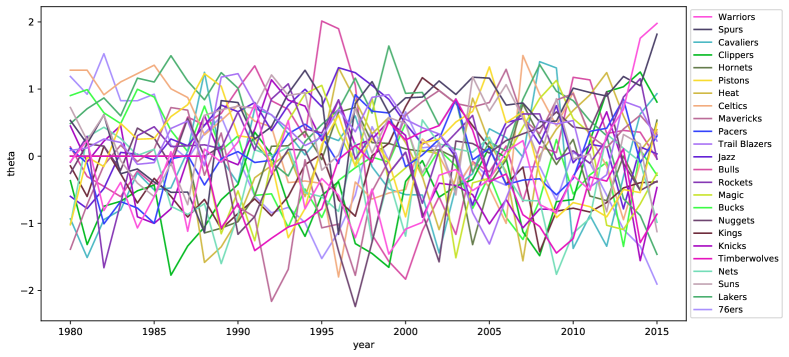
Figure 1: Path of $\hat{\bm{\theta}}(\mathcal{I}_{s})$ for $\mathcal{I}_{s}$ being each season of the NBA data.

To get a rough sense of the number and locations of change points, we check the paths of the logarithm of generalized likelihood ratio statistics, which are shown in Figure 2. It should be noted that although the GLR paths suggest the existence and locations of two change points, we cannot rely on these observation. This is because when multiple change points exist, there will be cancellations effects and the GLR paths may not give consistent estimates of change points (Venkatraman,, 1992). We can also see that splitting the data by odd and even indices does not affect the shape of the GLR path.

With all the information in the exploratory analysis, we apply our method DPLR to the dataset and summarize results in Section 5.

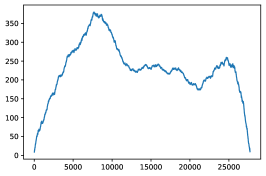
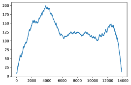
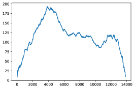
Figure 2: Path of (logarithmic) generalized loglikelihood ratio on NBA data. Left: GLR path on all samples; mid: GLR path on samples with odd indices; right: GLR path on samples with even indices.

A.3.2 Comparison with WBS-GLR

In this subsection, we apply the potential competitor, the likelihood-based WBS method (i.e. WBS-GLR), to the NBA data. For a fair comparison, we set the regularization tuning parameter $\gamma$ in the penalized logistic regression to be $0.1$, as we did in Section 5 for DPLR. However, as mentioned in Section A.1, WBS has another tuning parameter $M$, the number of random intervals to perform binary segmentation. So we apply WBS-GLR with $M\in\{50,100,150,200,250\}$, and the estimated change points with corresponding test errors (negative log-likelihoods) are summarized in Table 5. Here, we use samples with odd time indices as training data and even time indices as test data. It can be seen from Table 5 that the choice of $M$ does not have a significant impact on change point estimation in this real data example. Therefore in what follows, we only discuss the results of WBS-GLR with $M=200$.

$M$	Change point index	Change point season	Test errors
50	$[7728,14628,20700,24564]$	[S1990m, S1999, S2007, S2012]	1796.9
100	$[7728,14628,20700,24564]$	[S1990m, S1999, S2007, S2012]	1796.9
150	$[7728,14628,20700,24564]$	[S1990m, S1999, S2007, S2012]	1796.9
200	$[7728,14352,20700,24564]$	[S1990m, S1998m, S2007, S2012]	1793.2
250	$[7728,14628,20700,24564]$	[S1990m, S1999, S2007, S2012]	1796.9

Table 5: The estimated change points with testing loss of WBS-GLR on the NBA data. S1980 means season 1980-1981, and S1990m means the middle of season 1990-1991

Then similar to Section 5, we fit a BTL model to each interval segmented by WBS-GLR, and summarize the results in Table 6. As we can see, WBS-GLR is able to detect several important change points in the NBA history, e.g., the dominance of Celtics and Lakers in 1980s, the Bulls dynasty in 1990s, and the rise of Spurs afterwards. However, compared with DPLR, WBS-GLR fails to detect the rise of Heat and Warriors. Therefore, the outcome of DPLR is more informative in this real application, which again confirms our findings in the simulation study in Section 4.

S1980-S1990m		S1990m-S1998m		S1998m-S2006		S2007-S2011		S2012-S2015
Celtics	1.1137	Bulls	0.9435	Spurs	0.904	Lakers	0.7579	Spurs	1.1659
Lakers	1.084	Jazz	0.7996	Mavericks	0.665	Spurs	0.701	Clippers	0.9448
76ers	0.8049	Suns	0.5405	Lakers	0.5904	Celtics	0.6406	Warriors	0.9106
Bucks	0.7336	Knicks	0.5178	Kings	0.5103	Magic	0.6084	Heat	0.5149
Pistons	0.5074	Rockets	0.508	Suns	0.3677	Mavericks	0.605	Rockets	0.4703
Trail Blazers	0.4466	Trail Blazers	0.4931	Timberwolves	0.2767	Nuggets	0.458	Mavericks	0.3402
Suns	0.284	Spurs	0.4638	Pistons	0.2464	Bulls	0.2974	Pacers	0.3368
Nuggets	0.2294	Cavaliers	0.3415	Jazz	0.2266	Suns	0.28	Trail Blazers	0.2782
Bulls	0.1782	Lakers	0.3338	Pacers	0.1902	Rockets	0.2724	Bulls	0.2639
Jazz	0.1774	Pacers	0.241	Rockets	0.0024	Jazz	0.2499	Nuggets	0.0401
Spurs	0.1394	Magic	0.1824	Trail Blazers	-0.0049	Trail Blazers	0.1843	Jazz	-0.0495
Rockets	0.1252	Hornets	0.0923	Heat	-0.0433	Cavaliers	0.1628	Cavaliers	-0.0752
Mavericks	0.1004	Heat	0.0572	76ers	-0.0673	Hornets	0.0931	Celtics	-0.1486
Knicks	0.0744	Pistons	-0.1381	Nets	-0.0807	Heat	0.081	Hornets	-0.1522
Warriors	-0.1406	Warriors	-0.2101	Hornets	-0.113	76ers	-0.157	Nets	-0.2055
Nets	-0.1751	Celtics	-0.2326	Bucks	-0.2183	Pistons	-0.2651	Knicks	-0.2865
Pacers	-0.1857	Nets	-0.3088	Nuggets	-0.2676	Warriors	-0.3028	Suns	-0.296
Cavaliers	-0.2179	Bucks	-0.473	Magic	-0.2993	Pacers	-0.3475	Bucks	-0.354
Kings	-0.3197	Clippers	-0.5024	Knicks	-0.3218	Bucks	-0.4778	Pistons	-0.3591
Clippers	-0.6276	Kings	-0.5103	Celtics	-0.3293	Knicks	-0.6236	Kings	-0.4707
Timberwolves	-0.9485	Nuggets	-0.6578	Clippers	-0.4028	Clippers	-0.6919	Lakers	-0.5136
Hornets	-1.0599	Timberwolves	-0.6859	Cavaliers	-0.4321	Kings	-0.7288	Timberwolves	-0.5649
Magic	-1.1178	76ers	-0.7395	Warriors	-0.5857	Timberwolves	-0.8974	Magic	-0.697
Heat	-1.206	Mavericks	-1.056	Bulls	-0.8137	Nets	-0.8998	76ers	-1.093

Table 6: Fitted $\hat{\bm{\theta}}$ (rounded to the fourth decimal) for 24 selected teams in seasons 1980-2016 of the National Basketball Association. Teams are ranked by the MLE $\hat{\bm{\theta}}$ on subsets splitted at the estimated change points given by the WBS-GLR method. S1980 means season 1980-1981, and S1990m means the middle of season 1990-1991.

A.4 Other potential competitors

As we emphasized in Section 1 and Section 4, localizing potential change points in pairwise comparison data is an unsolved problem. Given the good performance of our proposed method DPLR in this paper, one might wonder if there exist other methods that perform well, or even better than DPLR, in some aspects. This section intends to present some of our explorations on two potential efficient methods, WBS-SST and WBS-Mean.

In what follows, we will demonstrate that both of them have crucial drawbacks. Specifically, WBS-Mean is not guaranteed to work for general comparison graphs, and works for general ranking models only under some constraints. WBS-SST works for general comparison graphs and ranking models, but requires relatively large sample size (i.e., $\Delta$) to work. Precise quantification of their performance can be an interesting direction for future works.

A.4.1 Based on the test statistic for SST class

Rastogi et al., (2020) consider the two sample testing problem for general pairwise comparison data. Suppose we observe pairwise comparison outcome matrices $\mathbf{X}$ and $\mathbf{Y}$ generated from two winning probability matrices $\mathbf{P},\mathbf{Q}\in\mathbb{R}^{n\times n}$, respectively. They propose the following test statistic:

$$R_{SST}=\sum_{i=1}^{d}\sum_{j=1}^{d}\mathbb{I}_{ij}\frac{k_{ij}^{q}\left(k_{ij}^{q}-1\right)\left(X_{ij}^{2}-X_{ij}\right)+k_{ij}^{p}\left(k_{ij}^{p}-1\right)\left(Y_{ij}^{2}-Y_{ij}\right)-2\left(k_{ij}^{p}-1\right)\left(k_{ij}^{q}-1\right)X_{ij}Y_{ij}}{\left(k_{ij}^{p}-1\right)\left(k_{ij}^{q}-1\right)\left(k_{ij}^{p}+k_{ij}^{q}\right)},$$ (A.3)

where $\mathbb{I}_{ij}=\mathbb{I}\left(k_{ij}^{p}>1\right)\times\mathbb{I}\left(k_{ij}^{q}>1\right)$, $k_{ij}^{p}=X_{ij}+X_{ji}$ and $k_{ij}^{q}=Y_{ij}+Y_{ji}$ are the number of comparisons between pairs.

We can use this test statistic to construct the loss $\mathcal{R}(t;s,e)$ in WBS (Algorithm 3), i.e.,

$$\mathcal{R}(t;s,e)=R_{SST}(\mathbf{X}([s,t)),\mathbf{Y}([t,e))),$$ (A.4)

and call this method WBS-SST (SST stands for strong stochastic transitive). When $\Delta$ is sufficiently large, WBS-SST performs fairly well with small computational cost, as is shown in Table 7.

Issue with this approach. However, When $\Delta$ is small, then many pairs in sampled intervals in WBS will have $k_{ij}\leq 1$, and the statistic would not be very powerful. See Figure 3 and Table 7.

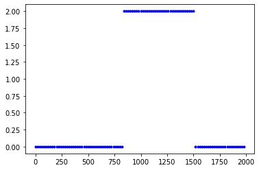
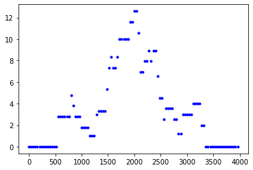
Figure 3: Loss path for WBS-SST when the sample size is not large enough. $n=100$ with a single change point at the middle. $\Delta=1000$ (left), $\Delta=2000$ (right).

To see that reason, notice that

$$\begin{split}\mathbb{E}[R_{SST}|\mathbf{k}^{p},\mathbf{k}^{q}]&=\sum_{i=1}^{d}\sum_{j=1}^{d}\mathbb{I}_{ij}\frac{k_{ij}^{q}\left(k_{ij}^{q}-1\right)k_{ij}^{p}\left(k_{ij}^{p}-1\right)(P_{ij}^{2}+Q_{ij}^{2}-2P_{ij}Q_{ij})}{\left(k_{ij}^{p}-1\right)\left(k_{ij}^{q}-1\right)\left(k_{ij}^{p}+k_{ij}^{q}\right)}\\ &=\sum_{i=1}^{d}\sum_{j=1}^{d}\mathbb{I}_{ij}\frac{k_{ij}^{q}k_{ij}^{p}}{k_{ij}^{p}+k_{ij}^{q}}(P_{ij}-Q_{ij})^{2}.\end{split}$$ (A.5)

When the comparison graph is a complete graph and compared pairs $\{(i_{t},j_{t})\}_{t\in[T]}$ are i.i.d. samples from the edge set $E_{full}:=\{(i,j):1\leq i<j\leq n\}$, the expectation of $R$ is (without the loss of generality, assume that $(1,2)\in E_{full}$)

$$\mathbb{E}[R_{SST}]=\|P-Q\|_{F}^{2}\mathbb{E}[\mathbb{I}_{1,2}\frac{k_{1,2}^{q}k_{1,2}^{p}}{k_{1,2}^{p}+k_{1,2}^{q}}].$$ (A.6)

The two equations above illustrate why WBS-SST does nor perform well in small-SNR cases.

A.4.2 Based on the Borda count

Borda count is a popular method in practice for ranking, due to its efficiency and generality (Shah and Wainwright,, 2018). Given an interval $\mathcal{I}$, the normalized Borda count vector is defined as

$$\beta(\mathcal{I})_{i}=\frac{1}{|\mathcal{I}|}[N_{w}(i;\mathcal{I})-N_{l}(i;\mathcal{I})],\forall i\in[n],$$ (A.7)

where $N_{w}(i;\mathcal{I})$ and $N_{l}(i;\mathcal{I})$ are the number of wining and loss of item $i$ in comparisons over the interval $\mathcal{I}$.

Since it is well-known in ranking literature that Borda count is not guaranteed to give consistent ranking for general comparison graphs, we only consider the complete graph here. When the comparison graph is a complete graph and compared pairs are i.i.d. samples from the edge set, and there is no change point in $\mathcal{I}$, the expectation of $\beta(\mathcal{I})_{i}$ is

$$\mathbb{E}[\beta(\mathcal{I})_{i}]=\frac{2}{n(n-1)}\sum_{j\neq i}(P_{ij}-P_{ji})=\frac{2}{n(n-1)}\sum_{j\neq i}(2P_{ij}-1),$$ (A.8)

where $P_{ij}=\mathbb{P}[i\text{ beats }j]$.

If we treat $\beta(\mathcal{I})$ as a sample mean of a random variable, we can construct the CUSUM statistic at $t\in\mathcal{I}=[s,e)$ as

$$\mathcal{R}_{Borda}(t;[s,e))=\frac{(t-s)(e-t)}{e-s}\|\bm{\beta}([s,t))-\bm{\beta}([t,e))\|_{2}^{2}.$$ (A.9)

To compared this statistic with Equation A.3, we assume there is a single change point $\eta\in[s,e)$ and check the statistic at $\eta$. By Equation A.8, the population version of the statistic is

$$\begin{split}\widetilde{\mathcal{R}}_{Borda}(\eta;[s,e))&=\frac{(\eta-s)(e-\eta)}{e-s}\|\mathbb{E}\bm{\beta}([s,\eta))-\mathbb{E}\bm{\beta}([\eta,e))\|_{2}^{2}\\ &=\frac{(\eta-s)(e-\eta)}{e-s}\cdot\frac{2}{n(n-1)}\sum_{i\in[n]}[\sum_{j\neq i}(P_{ij}-Q_{ij})]^{2}\end{split}$$ (A.10)

where $\mathbf{P},\mathbf{Q}$ are the winning probability matrices before and after the change point $\eta$.

Issue with this approach.

With Equation A.10, we can construct examples such that the population version of the CUSUM statistic is very small or even zero at the true change point $\eta$. For instance, let $n=3$ and

$$\mathbf{P}=\left[\begin{array}[]{ccc}0.5&0.6&0.8\\ 0.4&0.5&0.7\\ 0.2&0.3&0.5\end{array}\right],\quad\mathbf{Q}=\left[\begin{array}[]{ccc}0.5&0.55&0.85\\ 0.45&0.5&0.65\\ 0.15&0.35&0.5\end{array}\right],$$ (A.11)

then both $\mathbf{P},\mathbf{Q}$ are strong-stochastic-transitive matrices (see Shah and Wainwright, (2018) for details) and the population CUSUM $\widetilde{\mathcal{R}}_{Borda}(\eta;[s,e))=0$ at $\eta$. Figure 4 compares paths of the loss for WBS-Mean and WBS-SST under the choice of $\mathbf{P},\mathbf{Q}$ above, where there is a single change point at $\eta=1000$.

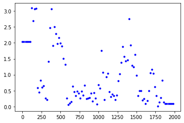
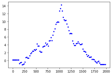
Figure 4: Loss path for WBS-Mean (left) and WBS-SST (right).

A.4.3 Numerical performance

Table 7 compares the performance of WBS-SST and WBS-Mean with the two methods presented in the main text, under the identical setting in Section 4. The setting is sketched below for convenience.

	$H(\hat{\eta},\eta)$	Time	$\hat{K}<K$	$\hat{K}=K$	$\hat{K}>K$
Setting (i)   $n=10,K=3,\Delta=500$, Change (I, II, III)
DPLR	9.2 (9.1)	49.7s (0.7)	0	100	0
WBS-Mean	15.4 (8.4)	0.2s (0.05)	0	100	0
WBS-SST	16.2 (11.4)	0.4s (0.2)	0	100	0
WBS-GLR	15.2 (7.9)	31.9s (3.9)	0	100	0
Setting (ii)   $n=20,K=3,\Delta=800$, Change (I, II, III)
DPLR	9.0 (9.9)	118.5s (2.2)	0	100	0
WBS-Mean	5.8 (11.4)	0.5s (0.1)	0	100	0
WBS-SST	19.4 (22.3)	1.7s (0.5)	0	100	0
WBS-GLR	240.5 (220.3)	144.2s (12.5)	0	40	60
Setting (iii)  $n=100,K=2,\Delta=1000$, Change (I, II)
DPLR	13.4 (14.4)	167.4s (3.3)	0	100	0
WBS-Mean	22.9 (98.4)	0.6s (0.04)	1	99	0
WBS-SST	$\infty$ (NA)	3.9s (0.4)	100	0	0
WBS-GLR	111.9 (195.6)	215.9s (17.0)	0	79	21
Setting (iv)   $n=100,K=3,\Delta=2000$, Change (I, II, III)
DPLR	12.4 (12.1)	402.4s (7.4)	0	100	0
WBS-Mean	17.9 (6.1)	0.9s (0.06)	0	100	0
WBS-SST	1116.3 (694.8)	19.3s (1.9)	57	42	1
WBS-GLR	412.3 (495.5)	400.0s (40.9)	0	57	43

Table 7: Comparison of DPLR and three WBS-based methods under four different simulation settings. 100 trials are conducted in each setting. For the localization error and running time (in seconds), the average over 100 trials is shown with standard error in the bracket. The three columns on the right record the number of trials in which $\hat{K}<K$, $\hat{K}=K$, and $\hat{K}>K$ respectively.

Simulation settings.

For $1<i\leq n$, we set $\theta_{i}^{*}(\eta_{0})=\theta_{1}^{*}(\eta_{0})+(i-1)\delta$ with some constant $\delta$. In each experiment, we set $\delta$ first and then set $\theta_{1}^{*}(\eta_{0})$ to make $\mathbf{1}^{\top}_{n}\bm{\theta}^{*}(\eta_{0})=0$. The value of $\delta$ guarantees that the maximum winning probability is 0.9. We consider three types of changes:

Type I (reverse): $\theta_{i}^{*}(\eta_{k})=\theta^{*}_{n+1-i}(\eta_{0})$.

Type II (block-reverse): $\theta_{i}^{*}(\eta_{k})=\theta^{*}_{[\frac{n}{2}]+1-i}(\eta_{0})$ for $i\leq[\frac{n}{2}]$; $\theta_{i}^{*}(\eta_{k})=\theta^{*}_{[\frac{n}{2}]+n+1-i}(\eta_{0})$ for $i>[\frac{n}{2}]$.

Type III (block exchange): $\theta_{i}^{*}(\eta_{k})=\theta^{*}_{i+[\frac{n}{2}]}(\eta_{0})$ for $i\leq[\frac{n}{2}]$; $\theta_{i}^{*}(\eta_{k})=\theta^{*}_{i-[\frac{n}{2}]}(\eta_{0})$ for $i>[\frac{n}{2}]$.

We consider four simulation settings. For each setting, we have $T=(K+1)\Delta$ and the change points locate at $\eta_{i}=i\Delta$ for $i\in[K]$. To describe the true parameter at each change point, we use an ordered tuple. For instance, (I, II, III, I) means that $K=4$ and the true parameters at $\eta_{1},\eta_{2},\eta_{3},\eta_{4}$ are determined based on $\bm{\theta}^{*}(\eta_{0})$ and the change type I, II, III, and I, respectively.

Appendix B Appendix: Proof

This section has three parts:

1. Section B.1 contains the proof of two theorems in Section 3.

2. Section B.2 contains propositions used throughout the paper with proof.

3. Section B.3 contains all technical lemmas with proof.

B.1 Proof of main theorems

Proof of Theorem 3.2.

The theorem is a straightforward conclusion of Proposition B.2 and Proposition B.1. More specifically, conclusion 3 and 4 of Proposition B.2 guarantee that $K\leq|\hat{\mathcal{P}}|\leq 3K$ with probability at least $1-(Tn)^{-2}$ and Proposition B.1 further confirms the consistency of $\hat{K}$. Then conclusion 1 and 2 of Proposition B.2 control the localization error. ∎

Proof of Theorem 3.3.

The theorem is a straightforward conclusion of Theorem 3.2 that quantifies the localization error of outputs of dynamic programming and Proposition B.3 that shows the improvement of local refinement. ∎

B.2 Main propositions

Proposition B.1 (Consistency of $\hat{K}$).

Let $\hat{\mathcal{P}}$ be the estimator of change points in Equation 3.1. Assume $K\leq|\hat{\mathcal{P}}|\leq 3K$. Under all assumptions above, it holds with probability at least $1-(Tn)^{-2}$ that $|\hat{\mathcal{P}}|=K$.

Proof.

For a sequence of strictly increasing integer time points $\{\eta_{j}^{\prime}\}_{j\in[J+1]}$ with $\eta_{0}^{\prime}=1$ and $\eta_{J+1}^{\prime}=T+1$, let $\mathcal{I}_{j}=[\eta_{j-1}^{\prime},\eta_{j}^{\prime})$ and

$$L(\{\eta_{j}^{\prime}\}_{j\in[J+1]})=\sum_{j\in[J+1]}L(\hat{\bm{\theta}}(\mathcal{I}_{j}),\mathcal{I}_{j}),$$

where $\hat{\bm{\theta}}(\mathcal{I}_{j}):=\operatornamewithlimits{arg\,min}_{\bm{\theta}\in\Theta_{B}}L({\bm{\theta}},\mathcal{I}_{j})$. Furthermore, when $\{\eta_{k}\}_{k\in[K]}\subset\{\eta_{j}^{\prime}\}_{j\in[J+1]}$ so that $\theta^{*}(t)$ remains unchanged in each interval $\mathcal{I}_{j}$, we can define the risk of true parameters

$$L^{*}(\{\eta_{j}^{\prime}\}_{j\in[J+1]})=\sum_{j\in[J+1]}L({\bm{\theta}}^{*}(\mathcal{I}_{j}),\mathcal{I}_{j}).$$

Let $\{\hat{\eta}_{k}\}_{k\in[\hat{K}]}$ be the change points given by the estimator $\hat{\mathcal{P}}$ and $\mathbf{Sort}(\cdot)$ be an operator on finite ordered tuple of scalars such that $\mathbf{Sort}((a_{1},\ldots,a_{m}))=(a_{(1)},\ldots,a_{(m)})$ where $a_{(i)}\leq a_{(j)}$ for $i<j$ and $\{a_{(i)}\}_{i\in[m]}=\{a_{i}\}_{i\in[m]}$. Then a sufficient condition for $|\hat{\mathcal{P}}|=K$ is

$$L^{*}(\eta_{1},\cdots,\eta_{K})+K\gamma$$

$$\geq L(\eta_{1},\cdots,\eta_{K})+K\gamma$$ (B.1)

$$\geq L(\hat{\eta}_{1},\cdots,\hat{\eta}_{\hat{K}})+\hat{K}\gamma$$ (B.2)

$$\geq L^{*}(\mathbf{Sort}(\hat{\eta}_{1},\cdots,\hat{\eta}_{\hat{K}},\eta_{1},\cdots,\eta_{K}))+\hat{K}\gamma-CKp_{lb}^{-2}\frac{nd_{\max}}{\lambda_{2}(L_{\mathcal{G}})}\log(Tn),$$ (B.3)

and

$$L^{*}(\eta_{1},\cdots,\eta_{K})\leq L^{*}(\mathbf{Sort}(\hat{\eta}_{1},\cdots,\hat{\eta}_{\hat{K}},\eta_{1},\cdots,\eta_{K}))+C_{1}Kp_{lb}^{-2}\frac{nd_{\max}}{\lambda_{2}(L_{\mathcal{G}})}\log(Tn).$$ (B.4)

In fact, if $\hat{K}\geq K+1$, under the conditions above and the assumption that $|\hat{\mathcal{P}}|\leq 3K$, we have

$$\gamma\leq(\hat{K}-K)\gamma\leq C_{2}Kp_{lb}^{-2}\frac{nd_{\max}}{\lambda_{2}(L_{\mathcal{G}})}\log(Tn),$$

which is contradictory to the definition $\gamma=C_{\gamma}(K+1)p_{lb}^{-2}\frac{nd_{\max}}{\lambda_{2}(L_{\mathcal{G}})}\log(Tn)$ for sufficiently large $C_{\gamma}$.

Now we prove that the sufficient condition holds with probability at least $1-(Tn)^{-2}$. Equation B.1 is a straightforward conclusion of the definition $\hat{\bm{\theta}}(\mathcal{I}_{j}):=\operatornamewithlimits{arg\,min}_{\bm{\theta}\in\Theta_{B}}L({\bm{\theta}},\mathcal{I}_{j})$ and Equation B.2 is implied by the definition of $\hat{\mathcal{P}}$ in Equation 3.1.

Equation B.4 is guaranteed by Lemma B.9 because for any interval $\mathcal{I}$ determined by endpoints that are two consecutive points in $\mathbf{Sort}(\hat{\eta}_{1},\cdots,\hat{\eta}_{\hat{K}},\eta_{1},\cdots,\eta_{K})$, there will not be any true change point in the interior of $\mathcal{I}$.

For Equation B.3, notice that by Proposition B.2, with probability $1-(Tn)^{-4}$, there are at most two change points in $\mathcal{I}$. Therefore, Lemma B.7 ensures that

$$L(\hat{\eta}_{1},\cdots,\hat{\eta}_{\hat{K}})\geq L^{*}(\mathbf{Sort}(\hat{\eta}_{1},\cdots,\hat{\eta}_{\hat{K}},\eta_{1},\cdots,\eta_{K}))-CKp_{lb}^{-2}\frac{nd_{\max}}{\lambda_{2}(L_{\mathcal{G}})}\log(Tn).$$

∎

Proposition B.2 (Four cases).

Let $\hat{\mathcal{P}}$ be the estimator of change points in Equation 3.1. Under Assumption 3.1 and Assumption B.14, with probability at least $1-(Tn)^{-2}$ the following four events hold uniformly for all $\mathcal{I}=(s,e)\in\hat{\mathcal{P}}$:

1. If $\mathcal{I}$ contains only one change point $\eta$, then for some universal constant $C>0$,

   $$\min\{\eta-s,e-\eta\}\leq Cp_{lb}^{-2}\frac{|E|}{\lambda_{2}(L_{\mathcal{G}})}[\gamma+\frac{nd_{\max}}{\lambda_{2}(L_{\mathcal{G}})}\log(Tn)].$$

2. If $\mathcal{I}$ contains exactly two change points $\eta_{k}$ and $\eta_{k+1}$, then for some universal constant $C>0$,

   $$\min\{\eta_{k}-s,e-\eta_{k+1}\}\leq Cp_{lb}^{-2}\frac{|E|}{\lambda_{2}(L_{\mathcal{G}})}[\gamma+\frac{nd_{\max}}{\lambda_{2}(L_{\mathcal{G}})}\log(Tn)].$$

3. If $|\hat{\mathcal{P}}|>1$, then for any two consecutive intervals $\mathcal{I}$ and $\mathcal{J}$ in $\hat{\mathcal{P}}$, the joint interval $\mathcal{I}\cup\mathcal{J}$ contains at least one change point.

4. Interval $\mathcal{I}$ does not contain more than two change points.

Proof.

Conclusion 1 is implied by Lemma B.11 and conclusion 2 is guaranteed by Lemma B.12. Conclusion 4 is a direct consequence of Lemma B.13 and the definition of $\hat{\mathcal{P}}$.

To prove conclusion 3, assume instead that there is no true change point in $\mathcal{I}\cup\mathcal{J}$. Then by Lemma B.10 we have

$$L(\hat{\bm{\theta}}(\mathcal{I}),\mathcal{I})+L(\hat{\bm{\theta}}(\mathcal{J}),\mathcal{J})+\gamma\geq L({\bm{\theta}}^{*}(\mathcal{I}\cup\mathcal{J}),\mathcal{I}\cup\mathcal{J})\geq L(\hat{\bm{\theta}}(\mathcal{I}\cup\mathcal{J}),\mathcal{I}\cup\mathcal{J}),$$

which is contradictory to the definition of $\hat{\mathcal{P}}$. ∎

Proposition B.3 (Local refinement).

Consider the local refinement procedure given in Algorithm 2, that is,

$$\left(\hat{\eta}_{k},\hat{\bm{\theta}}^{(1)},\hat{\bm{\theta}}^{(2)}\right)=\operatornamewithlimits{arg\,min}_{\begin{subarray}{c}\eta\in\{s_{k}+1,\ldots,e_{k}-1\}\\ \bm{\theta}^{(1)},\bm{\theta}^{(2)}\in\Theta_{B}\end{subarray}}\Bigg{\{}\sum_{t=s_{k}+1}^{\eta}\ell_{t}(\bm{\theta}^{(1)})+\sum_{t=\eta+1}^{e_{k}}\ell_{t}(\bm{\theta}^{(2)})\Bigg{\}},$$ (B.5)

where $s_{k}=2\widetilde{\eta}_{k-1}/3+\widetilde{\eta}_{k}/3$ and $e_{k}=\widetilde{\eta}_{k}/3+2\widetilde{\eta}_{k+1}/3$ and $\ell_{t}(\bm{\theta})$ is the negative log-likelihood given in Equation 2.6. Suppose the input $\{\tilde{\eta}_{k}\}_{k\in[\tilde{K}]}$ satisfies $\tilde{K}=K$ and

$$\max_{k\in[K]}|\tilde{\eta}_{k}-\eta_{k}|\leq\Delta/5.$$

Let $\{\hat{\eta}_{k}\}_{k\in[K]}$ be the output. Then it holds with probability at least $1-(Tn)^{-2}$ that

$$\max_{k\in[K]}|\hat{\eta}_{k}-\eta_{k}|\leq C\frac{|E|nd_{\max}}{p_{lb}^{2}\kappa^{2}\lambda_{2}^{2}(L_{\mathcal{G}})}\log(Tn).$$ (B.6)

Proof.

For each $k\in[K]$, let $\hat{\bm{\theta}}(t)=\hat{\bm{\theta}}^{(1)}$ if $s_{k}<t\leq\hat{\eta}_{k}$ and $\hat{\bm{\theta}}(t)=\hat{\bm{\theta}}^{(2)}$ otherwise, and ${\bm{\theta}}^{*}(t)$ be the true parameter at time point $t$. First we show that under conditions $\tilde{K}=K$ and $\max_{k\in[K]}|\tilde{\eta}_{k}-\eta_{k}|\leq\Delta/5$, there is only one true change point $\eta_{k}$ in $(s_{k},e_{k})$. It suffices to show that

$$|\tilde{\eta}_{k}-\eta_{k}|\leq\frac{2}{3}(\tilde{\eta}_{k+1}-\tilde{\eta}_{k}),\ \text{and}\ |\tilde{\eta}_{k+1}-\eta_{k+1}|\leq\frac{1}{3}(\tilde{\eta}_{k+1}-\tilde{\eta}_{k}).$$ (B.7)

Denote $R=\max_{k\in[K]}|\tilde{\eta}_{k}-\eta_{k}|$, then

$$\tilde{\eta}_{k+1}-\tilde{\eta}_{k} =\tilde{\eta}_{k+1}-{\eta}_{k+1}+{\eta}_{k+1}-{\eta}_{k}+{\eta}_{k}-\tilde{\eta}_{k}$$

$$=({\eta}_{k+1}-{\eta}_{k})+(\tilde{\eta}_{k+1}-{\eta}_{k+1})+({\eta}_{k}-\tilde{\eta}_{k})\in[{\eta}_{k+1}-{\eta}_{k}-2R,{\eta}_{k+1}-{\eta}_{k}+2R].$$

Therefore, Equation B.7 is guaranteed as long as

$$R\leq\frac{1}{3}(\Delta-2R),$$

which is equivalent to $R\leq\Delta/5$.

Now without loss of generality, assume that $s_{k}<\eta_{k}<\hat{\eta}_{k}<e_{k}$. Denote $\mathcal{I}_{k}=\{s_{k}+1,\cdots,e_{k}\}$. Consider two cases:

Case 1 If

$$\hat{\eta}_{k}-\eta_{k}<\max\{Cp_{lb}^{-2}\frac{|E|nd_{\max}}{\lambda_{2}^{2}(L_{\mathcal{G}})}\log(Tn),Cp_{lb}^{-2}\log(Tn)/\kappa^{2}\},$$

then the proof is done.

Case 2 If

$$\hat{\eta}_{k}-\eta_{k}\geq\max\{Cp_{lb}^{-2}\frac{|E|nd_{\max}}{\lambda_{2}^{2}(L_{\mathcal{G}})}\log(Tn),Cp_{lb}^{-2}\log(Tn)/\kappa^{2}\},$$

then we proceed to prove that $|\hat{\eta}_{k}-\eta_{k}|\leq C_{1}\frac{|E|nd_{\max}}{p_{lb}^{2}\kappa^{2}\lambda_{2}^{2}(L_{\mathcal{G}})}\log(Tn)$ with probability at least $1-(Tn)^{-3}$. Then we either prove the result or get an contradiction, and complete the proof in either case.

By the definition of $\hat{\eta}_{k},\hat{\bm{\theta}}^{(1)}$, and $\hat{\bm{\theta}}^{(2)}$, we have

$$\sum_{t\in\mathcal{I}_{k}}\ell_{t}(\hat{\bm{\theta}}(t))\leq\sum_{t\in\mathcal{I}_{k}}\ell_{t}({\bm{\theta}}^{*}(t)).$$

By Lemma B.8, this implies that

$$ce^{-2B}\sum_{t\in\mathcal{I}_{k}}[\mathbf{x}(t)^{\top}\Delta(t)]^{2}\leq\sum_{t\in\mathcal{I}_{k}}\epsilon_{t}\mathbf{x}(t)^{\top}\Delta(t),$$ (B.8)

where $\Delta(t):=\hat{\bm{\theta}}(t)-\bm{\theta}^{*}(t)$ and $\epsilon_{t}:=y_{t}-\frac{\exp(\mathbf{x}(t)^{\top}\bm{\theta}^{*}(t))}{1+\exp(\mathbf{x}(t)^{\top}\bm{\theta}^{*}(t))}$. For the cross term, by Lemma B.19 we have

$$\sum_{t\in\mathcal{I}_{k}}\epsilon_{t}\mathbf{x}(t)^{\top}\Delta(t) =\sum_{i\in[n]}\{\left|\frac{\sum_{t\in\mathcal{I}_{k}}\epsilon_{t}x_{i}(t)\Delta_{i}(t)}{\mathchoice{{\hbox{$\displaystyle\sqrt{\sum_{t\in\mathcal{I}_{k}}\Delta_{i}(t)^{2}\,}$}\lower 0.4pt\hbox{\vrule height=9.30444pt,depth=-7.44359pt}}}{{\hbox{$\textstyle\sqrt{\sum_{t\in\mathcal{I}_{k}}\Delta_{i}(t)^{2}\,}$}\lower 0.4pt\hbox{\vrule height=9.30444pt,depth=-7.44359pt}}}{{\hbox{$\scriptstyle\sqrt{\sum_{t\in\mathcal{I}_{k}}\Delta_{i}(t)^{2}\,}$}\lower 0.4pt\hbox{\vrule height=6.53888pt,depth=-5.23112pt}}}{{\hbox{$\scriptscriptstyle\sqrt{\sum_{t\in\mathcal{I}_{k}}\Delta_{i}(t)^{2}\,}$}\lower 0.4pt\hbox{\vrule height=5.03888pt,depth=-4.03113pt}}}}\right|\mathchoice{{\hbox{$\displaystyle\sqrt{\sum_{t\in\mathcal{I}_{k}}\Delta_{i}(t)^{2}\,}$}\lower 0.4pt\hbox{\vrule height=9.30444pt,depth=-7.44359pt}}}{{\hbox{$\textstyle\sqrt{\sum_{t\in\mathcal{I}_{k}}\Delta_{i}(t)^{2}\,}$}\lower 0.4pt\hbox{\vrule height=9.30444pt,depth=-7.44359pt}}}{{\hbox{$\scriptstyle\sqrt{\sum_{t\in\mathcal{I}_{k}}\Delta_{i}(t)^{2}\,}$}\lower 0.4pt\hbox{\vrule height=6.53888pt,depth=-5.23112pt}}}{{\hbox{$\scriptscriptstyle\sqrt{\sum_{t\in\mathcal{I}_{k}}\Delta_{i}(t)^{2}\,}$}\lower 0.4pt\hbox{\vrule height=5.03888pt,depth=-4.03113pt}}}\}$$

$$\leq\sup_{i\in[n]}\left|\frac{\sum_{t\in\mathcal{I}_{k}}\epsilon_{t}x_{i}(t)\Delta_{i}(t)}{\mathchoice{{\hbox{$\displaystyle\sqrt{\sum_{t\in\mathcal{I}_{k}}\Delta_{i}(t)^{2}\,}$}\lower 0.4pt\hbox{\vrule height=9.30444pt,depth=-7.44359pt}}}{{\hbox{$\textstyle\sqrt{\sum_{t\in\mathcal{I}_{k}}\Delta_{i}(t)^{2}\,}$}\lower 0.4pt\hbox{\vrule height=9.30444pt,depth=-7.44359pt}}}{{\hbox{$\scriptstyle\sqrt{\sum_{t\in\mathcal{I}_{k}}\Delta_{i}(t)^{2}\,}$}\lower 0.4pt\hbox{\vrule height=6.53888pt,depth=-5.23112pt}}}{{\hbox{$\scriptscriptstyle\sqrt{\sum_{t\in\mathcal{I}_{k}}\Delta_{i}(t)^{2}\,}$}\lower 0.4pt\hbox{\vrule height=5.03888pt,depth=-4.03113pt}}}}\right|\sum_{i\in[n]}\mathchoice{{\hbox{$\displaystyle\sqrt{\sum_{t\in\mathcal{I}_{k}}\Delta_{i}(t)^{2}\,}$}\lower 0.4pt\hbox{\vrule height=9.30444pt,depth=-7.44359pt}}}{{\hbox{$\textstyle\sqrt{\sum_{t\in\mathcal{I}_{k}}\Delta_{i}(t)^{2}\,}$}\lower 0.4pt\hbox{\vrule height=9.30444pt,depth=-7.44359pt}}}{{\hbox{$\scriptstyle\sqrt{\sum_{t\in\mathcal{I}_{k}}\Delta_{i}(t)^{2}\,}$}\lower 0.4pt\hbox{\vrule height=6.53888pt,depth=-5.23112pt}}}{{\hbox{$\scriptscriptstyle\sqrt{\sum_{t\in\mathcal{I}_{k}}\Delta_{i}(t)^{2}\,}$}\lower 0.4pt\hbox{\vrule height=5.03888pt,depth=-4.03113pt}}}$$

$$\leq C\mathchoice{{\hbox{$\displaystyle\sqrt{\frac{d_{\max}}{|E|}\log(Tn)\,}$}\lower 0.4pt\hbox{\vrule height=13.15pt,depth=-10.52005pt}}}{{\hbox{$\textstyle\sqrt{\frac{d_{\max}}{|E|}\log(Tn)\,}$}\lower 0.4pt\hbox{\vrule height=9.22221pt,depth=-7.3778pt}}}{{\hbox{$\scriptstyle\sqrt{\frac{d_{\max}}{|E|}\log(Tn)\,}$}\lower 0.4pt\hbox{\vrule height=6.83333pt,depth=-5.46669pt}}}{{\hbox{$\scriptscriptstyle\sqrt{\frac{d_{\max}}{|E|}\log(Tn)\,}$}\lower 0.4pt\hbox{\vrule height=6.83333pt,depth=-5.46669pt}}}\sum_{i\in[n]}\mathchoice{{\hbox{$\displaystyle\sqrt{\sum_{t\in\mathcal{I}_{k}}(\hat{\theta}_{i}-\theta^{*}_{i}(t))^{2}\,}$}\lower 0.4pt\hbox{\vrule height=9.30444pt,depth=-7.44359pt}}}{{\hbox{$\textstyle\sqrt{\sum_{t\in\mathcal{I}_{k}}(\hat{\theta}_{i}-\theta^{*}_{i}(t))^{2}\,}$}\lower 0.4pt\hbox{\vrule height=9.30444pt,depth=-7.44359pt}}}{{\hbox{$\scriptstyle\sqrt{\sum_{t\in\mathcal{I}_{k}}(\hat{\theta}_{i}-\theta^{*}_{i}(t))^{2}\,}$}\lower 0.4pt\hbox{\vrule height=7.22223pt,depth=-5.77782pt}}}{{\hbox{$\scriptscriptstyle\sqrt{\sum_{t\in\mathcal{I}_{k}}(\hat{\theta}_{i}-\theta^{*}_{i}(t))^{2}\,}$}\lower 0.4pt\hbox{\vrule height=7.22223pt,depth=-5.77782pt}}}$$

$$\leq C\mathchoice{{\hbox{$\displaystyle\sqrt{\frac{nd_{\max}}{|E|}\log(Tn)\,}$}\lower 0.4pt\hbox{\vrule height=13.15pt,depth=-10.52005pt}}}{{\hbox{$\textstyle\sqrt{\frac{nd_{\max}}{|E|}\log(Tn)\,}$}\lower 0.4pt\hbox{\vrule height=9.22221pt,depth=-7.3778pt}}}{{\hbox{$\scriptstyle\sqrt{\frac{nd_{\max}}{|E|}\log(Tn)\,}$}\lower 0.4pt\hbox{\vrule height=6.83333pt,depth=-5.46669pt}}}{{\hbox{$\scriptscriptstyle\sqrt{\frac{nd_{\max}}{|E|}\log(Tn)\,}$}\lower 0.4pt\hbox{\vrule height=6.83333pt,depth=-5.46669pt}}}\mathchoice{{\hbox{$\displaystyle\sqrt{\sum_{t\in\mathcal{I}_{k}}\|\Delta(t)\|_{2}^{2}\,}$}\lower 0.4pt\hbox{\vrule height=9.30444pt,depth=-7.44359pt}}}{{\hbox{$\textstyle\sqrt{\sum_{t\in\mathcal{I}_{k}}\|\Delta(t)\|_{2}^{2}\,}$}\lower 0.4pt\hbox{\vrule height=9.30444pt,depth=-7.44359pt}}}{{\hbox{$\scriptstyle\sqrt{\sum_{t\in\mathcal{I}_{k}}\|\Delta(t)\|_{2}^{2}\,}$}\lower 0.4pt\hbox{\vrule height=6.53888pt,depth=-5.23112pt}}}{{\hbox{$\scriptscriptstyle\sqrt{\sum_{t\in\mathcal{I}_{k}}\|\Delta(t)\|_{2}^{2}\,}$}\lower 0.4pt\hbox{\vrule height=5.03888pt,depth=-4.03113pt}}}.$$ (B.9)

Equation B.8 and Equation B.9 together imply that

$$ce^{-2B}\sum_{t\in\mathcal{I}_{k}}[\mathbf{x}(t)^{\top}\Delta(t)]^{2}\leq C\mathchoice{{\hbox{$\displaystyle\sqrt{\frac{nd_{\max}}{|E|}\log(Tn)\,}$}\lower 0.4pt\hbox{\vrule height=13.15pt,depth=-10.52005pt}}}{{\hbox{$\textstyle\sqrt{\frac{nd_{\max}}{|E|}\log(Tn)\,}$}\lower 0.4pt\hbox{\vrule height=9.22221pt,depth=-7.3778pt}}}{{\hbox{$\scriptstyle\sqrt{\frac{nd_{\max}}{|E|}\log(Tn)\,}$}\lower 0.4pt\hbox{\vrule height=6.83333pt,depth=-5.46669pt}}}{{\hbox{$\scriptscriptstyle\sqrt{\frac{nd_{\max}}{|E|}\log(Tn)\,}$}\lower 0.4pt\hbox{\vrule height=6.83333pt,depth=-5.46669pt}}}\mathchoice{{\hbox{$\displaystyle\sqrt{\sum_{t\in\mathcal{I}_{k}}\|\Delta(t)\|_{2}^{2}\,}$}\lower 0.4pt\hbox{\vrule height=9.30444pt,depth=-7.44359pt}}}{{\hbox{$\textstyle\sqrt{\sum_{t\in\mathcal{I}_{k}}\|\Delta(t)\|_{2}^{2}\,}$}\lower 0.4pt\hbox{\vrule height=9.30444pt,depth=-7.44359pt}}}{{\hbox{$\scriptstyle\sqrt{\sum_{t\in\mathcal{I}_{k}}\|\Delta(t)\|_{2}^{2}\,}$}\lower 0.4pt\hbox{\vrule height=6.53888pt,depth=-5.23112pt}}}{{\hbox{$\scriptscriptstyle\sqrt{\sum_{t\in\mathcal{I}_{k}}\|\Delta(t)\|_{2}^{2}\,}$}\lower 0.4pt\hbox{\vrule height=5.03888pt,depth=-4.03113pt}}}.$$ (B.10)

Let

$$\mathcal{J}_{1}=(s_{k},\eta_{k}],\ \mathcal{J}_{2}=(\eta_{k},\hat{\eta}_{k}],\ \mathcal{J}_{3}=(\hat{\eta}_{k},e_{k}].$$

Under Assumption 3.1 and the condition of the proposition, it holds that $\min\{|\mathcal{J}_{1}|,|\mathcal{J}_{3}|\}\geq C_{0}\frac{|E|\log(Tn)}{\lambda_{2}(L_{\mathcal{G}})}$. Thus, by Lemma B.17, with probability at leat $1-(Tn)^{-3}$, we have

$$\sum_{t\in\mathcal{I}_{k}}[\mathbf{x}(t)^{\top}\Delta(t)]^{2}\geq\frac{c_{1}\lambda_{2}(L_{\mathcal{G}})}{|E|}\sum_{t\in\mathcal{I}_{k}}\|\Delta(t)\|_{2}^{2}.$$

The inequality above leads to

$$\sum_{t\in\mathcal{I}_{k}}\|\hat{\bm{\theta}}(t)-\bm{\theta}^{*}(t)\|_{2}^{2}\leq Cp_{lb}^{-2}\frac{|E|nd_{\max}}{\lambda_{2}^{2}(L_{\mathcal{G}})}\log(Tn).$$

Recall that we defined $\bm{\theta}^{(1)}=\bm{\theta}^{*}({\eta_{k}-1})$ and $\bm{\theta}^{(2)}=\bm{\theta}^{*}({\eta_{k}})$. Then we have

$$\sum_{t\in\mathcal{I}_{k}}\|\hat{\bm{\theta}}(t)-\bm{\theta}^{*}(t)\|_{2}^{2}=|\mathcal{J}_{1}|\|\hat{\bm{\theta}}^{(1)}-\bm{\theta}^{(1)}\|_{2}^{2}+|\mathcal{J}_{2}|\|\hat{\bm{\theta}}^{(1)}-\bm{\theta}^{(2)}\|_{2}^{2}+|\mathcal{J}_{3}|\|\hat{\bm{\theta}}^{(2)}-\bm{\theta}^{(2)}\|_{2}^{2}.$$

Since $|\mathcal{J}_{1}|=\eta_{k}-s_{k}\geq c_{0}\Delta$ with some constant $c_{0}$ under Assumption 3.1, we have

$$\Delta\|\hat{\bm{\theta}}^{(1)}-\bm{\theta}^{(1)}\|_{2}^{2}\leq c_{0}|\mathcal{J}_{1}|\|\hat{\bm{\theta}}^{(1)}-\bm{\theta}^{(1)}\|_{2}^{2}\leq c_{1}p_{lb}^{-2}\frac{|E|nd_{\max}}{\lambda_{2}^{2}(L_{\mathcal{G}})}\log(Tn)\leq c_{2}\Delta\kappa^{2},$$ (B.11)

with some constant $c_{2}\in(0,1/4)$, where the last inequality is due to the fact that $\mathcal{B}_{T}\rightarrow\infty$. Thus we have

$$\|\hat{\bm{\theta}}^{(1)}-\bm{\theta}^{(1)}\|_{2}^{2}\leq c_{2}\kappa^{2}.$$

Triangle inequality gives

$$\|\hat{\bm{\theta}}^{(1)}-\bm{\theta}^{(2)}\|_{2}\geq\|\bm{\theta}^{(1)}-\bm{\theta}^{(2)}\|_{2}-\|\hat{\bm{\theta}}^{(1)}-\bm{\theta}^{(1)}\|_{2}\geq\kappa/2.$$

Therefore, $\kappa^{2}|\mathcal{J}_{2}|/4\leq|\mathcal{J}_{2}|\|\hat{\bm{\theta}}^{(1)}-\bm{\theta}^{(2)}\|_{2}^{2}\leq Cp_{lb}^{-2}\frac{|E|nd_{\max}}{\lambda_{2}^{2}(L_{\mathcal{G}})}\log(Tn)$ and

$$|\hat{\eta}_{k}-\eta_{k}|=|\mathcal{J}_{2}|\leq\frac{Cp_{lb}^{-2}|E|nd_{\max}\log(Tn)}{\lambda_{2}^{2}(L_{\mathcal{G}})\kappa^{2}}.$$

∎

Proposition B.4.

Let $\mathbf{P}(\bm{\theta})$ be the winning probability matrix induced by $\bm{\theta}$. For $\bm{\theta}^{(1)},\bm{\theta}^{(2)}\in\Theta_{B}$, it holds that

$$\frac{np^{2}_{lb}}{16}\|\bm{\theta}^{(1)}-\bm{\theta}^{(2)}\|_{2}^{2}\leq\|\mathbf{P}(\bm{\theta}^{(1)})-\mathbf{P}(\bm{\theta}^{(2)})\|_{F}^{2}\leq\frac{n}{16}\|\bm{\theta}^{(1)}-\bm{\theta}^{(2)}\|_{2}^{2},$$ (B.12)

where $p_{lb}=\frac{e^{-2B}}{1+e^{-2B}}$.

Proof.

This result has been shown in Shah and Wainwright, (2018) (In the proof of Theorem 4). We include it here for completeness.

Denote $\psi(t)=\frac{1}{1+e^{-t}}$. For any pair $(i,j)\in[n]^{2}$, by the mean value theorem we have

$$|P_{ij}(\bm{\theta}^{(1)})-P_{ij}(\bm{\theta}^{(2)})| =|\psi(\theta^{(1)}_{i}-\theta^{(1)}_{j})-\psi(\theta^{(2)}_{i}-\theta^{(2)}_{j})|$$

$$=|\psi^{\prime}(\xi)||(\theta^{(1)}_{i}-\theta^{(1)}_{j})-(\theta^{(2)}_{i}-\theta^{(2)}_{j})|,$$

where $\xi$ is a scalar between $(\theta^{(1)}_{i}-\theta^{(1)}_{j})$ and $(\theta^{(2)}_{i}-\theta^{(2)}_{j})$. Since $\psi^{\prime}(t)=\psi(t)(1-\psi(t))\in(\frac{1}{4e^{2B}},\frac{1}{4}]$ for $t\in[-2B,2B]$, we have

$$\frac{1}{4e^{2B}}|(\theta^{(1)}_{i}-\theta^{(1)}_{j})-(\theta^{(2)}_{i}-\theta^{(2)}_{j})|\leq|P_{ij}(\bm{\theta}^{(1)})-P_{ij}(\bm{\theta}^{(2)})|\leq\frac{1}{4}|(\theta^{(1)}_{i}-\theta^{(1)}_{j})-(\theta^{(2)}_{i}-\theta^{(2)}_{j})|.$$

By the property of Graph Laplacian and the fact that $\mathbf{1}_{n}^{\top}\bm{\theta}^{(i)}=0$, $i=1,2$, we have

$$\sum_{i,j\in[n]^{2}}[(\theta^{(1)}_{i}-\theta^{(1)}_{j})-(\theta^{(2)}_{i}-\theta^{(2)}_{j})]^{2} =(\bm{\theta}^{(1)}-\bm{\theta}^{(2)})^{\top}[n\mathbf{I}_{n}-\mathbf{1}_{n}\mathbf{1}_{n}^{\top}](\bm{\theta}^{(1)}-\bm{\theta}^{(2)})$$ (B.13)

$$=n\|\bm{\theta}^{(1)}-\bm{\theta}^{(2)}\|_{2}^{2}.$$ (B.14)

Combining the results above gives the conclusion. ∎

Proposition B.5 (Single change point).

Suppose we observe $\{(\mathbf{x}(t),y_{t})\}_{t\in[T]}$ following model (2.1) and (2.5) and there is a single change point $\eta\in(1,T)$. In addition, assume that

$$\Delta:=\min\{\eta-1,T-\eta\}\geq\mathcal{B}_{T}\frac{|E|nd_{\max}}{p_{lb}^{2}\kappa^{2}\lambda_{2}^{2}(L_{\mathcal{G}})}\log(Tn),$$ (B.15)

for a diverging sequence $\{\mathcal{B}_{T}\}_{T\in\mathbb{Z}_{+}}$. Let the estimator $\hat{\eta}$ of the change point be

$$\hat{\eta}=\operatornamewithlimits{arg\,min}_{\eta\in[T]}\Bigg{\{}\min_{\bm{\theta}^{(1)}\in\Theta_{B}}\sum_{t=1}^{\eta}\ell_{t}(\bm{\theta}^{(1)})+\min_{\bm{\theta}^{(2)}\in\Theta_{B}}\sum_{t=\eta+1}^{T}\ell_{t}(\bm{\theta}^{(2)})\Bigg{\}},$$ (B.16)

where $\ell_{t}(\bm{\theta})$ is the negative log-likelihood given in Equation 2.6. Then it holds with probability at least $1-(Tn)^{-2}$ that

$$|\hat{\eta}-\eta|\leq\frac{Cp_{lb}^{-2}|E|nd_{\max}\log(Tn)}{\lambda_{2}^{2}(L_{\mathcal{G}})\kappa^{2}}.$$ (B.17)

Proof.

The estimator $\hat{\eta}$ is the same as the output of the local refinement algorithm. Under the assumption (B.15), the same arguments in the proof of Proposition B.3 can be applied here to show the conclusion.

It should be noted that the estimator $\hat{\eta}$ gives consistent localization because as $T\rightarrow\infty$, we have $\mathcal{B}_{T}\rightarrow\infty$ and with high probability,

$$\frac{|\hat{\eta}-\eta|}{\Delta}\leq\frac{C}{\mathcal{B}_{T}}=o(1).$$

∎

Proposition B.6 (No change point).

Suppose we observe $\{(\mathbf{x}(t),y_{t})\}_{t\in[T]}$ following model (2.1) and (2.5) and there is no single change point in $[1,T]$. In addition, assume that

$$T\geq\mathcal{B}_{T}\frac{|E|nd_{\max}}{p_{lb}^{2}\kappa^{2}\lambda_{2}^{2}(L_{\mathcal{G}})}\log(Tn),$$ (B.18)

for a diverging sequence $\{\mathcal{B}_{T}\}_{T\in\mathbb{Z}_{+}}$. Then it holds with probability at least $1-(Tn)^{-2}$ that the DP procedure in Algorithm 1 with tuning parameter $\gamma=C_{\gamma}p_{lb}^{-2}\frac{nd_{\max}}{\lambda_{2}(L_{\mathcal{G}})}\log(Tn)$ will return an empty set.

Proof.

Assume that the output $\hat{\mathcal{P}}=\{\hat{\eta}_{k}\}_{k\in[\hat{K}]}$ with $\hat{K}\geq 1$. Let $\mathcal{I}_{0}=[1,\hat{\eta}_{1})$ and $\mathcal{I}_{\hat{K}}=[\hat{\eta}_{\hat{K}},T]$. When ${\hat{K}}>1$, let $\mathcal{I}_{k}=[\hat{\eta}_{k-1},\hat{\eta}_{k})$ for $k\in[{\hat{K}}-1]$. Then by Lemma B.9, with probability at least $1-(Tn)^{-4}$, we have

$$\sum_{k=0}^{{\hat{K}}}L(\hat{\bm{\theta}}(\mathcal{I}_{k}),\mathcal{I}_{k})+{\hat{K}}Cp_{lb}^{-2}\frac{nd_{\max}}{\lambda_{2}(L_{\mathcal{G}})}\log(Tn) \geq\sum_{k=0}^{{\hat{K}}}L({\bm{\theta}}^{*}(\mathcal{I}_{k}),\mathcal{I}_{k})$$

$$=L({\bm{\theta}}^{*}([1,T]),[1,T])\geq L(\hat{\bm{\theta}}([1,T]),[1,T]),$$

which is contradictory to the definition of $\hat{\mathcal{P}}$ as long as $C_{\gamma}>C$. ∎

B.3 Technical lemmas

This section has three parts:

1. Lemma B.7 is a summary of three different cases, and is used in the proof of Proposition B.1.

2. Section B.3.1 contains results on the excess risk of $L(\bm{\theta}(\mathcal{I}),\mathcal{I})$ in four cases.

3. Section B.3.2 contains lemmas on some basic concentration properties related to our problem.

Lemma B.7.

Given any interval $\mathcal{I}=(s,e]\subset[1,T]$ with integers $s,e$ that contains at most two change points. Under all assumptions above, we have

1. If $\mathcal{I}$ contains no change points, then with probability at leat $1-(Tn)^{-2}$ it holds that

   $$L(\bm{\theta}^{*}(\mathcal{I}),\mathcal{I})\leq L(\hat{\bm{\theta}}(\mathcal{I}),\mathcal{I})+Cp_{lb}^{-2}\frac{nd_{\max}}{\lambda_{2}(L_{\mathcal{G}})}\log(Tn).$$

2. If $\mathcal{I}$ contains exactly one change point $\eta_{r}$ with partition $\mathcal{I}_{1}=(s,\eta_{r}]$ and $\mathcal{I}_{2}=(\eta_{r},e]$, then with probability at leat $1-(Tn)^{-2}$ it holds that

   $$L(\bm{\theta}^{*}(\mathcal{I}_{1}),\mathcal{I}_{1})+L(\bm{\theta}^{*}(\mathcal{I}_{2}),\mathcal{I}_{2})\leq L(\hat{\bm{\theta}}(\mathcal{I}),\mathcal{I})+Cp_{lb}^{-2}\frac{nd_{\max}}{\lambda_{2}(L_{\mathcal{G}})}\log(Tn).$$

3. If $\mathcal{I}$ contains exactly two change points $\eta_{r+1}$ and $\eta_{r+2}$ with partition $\mathcal{I}_{1}=(s,\eta_{r+1}]$, $\mathcal{I}_{2}=(\eta_{r+1},\eta_{r+2}]$, and $\mathcal{I}_{3}=(\eta_{r+2},e]$, then with probability at leat $1-(Tn)^{-2}$ it holds that

   $$\sum_{j=1}^{3}L(\bm{\theta}^{*}(\mathcal{I}_{j}),\mathcal{I}_{j})\leq L(\hat{\bm{\theta}}(\mathcal{I}),\mathcal{I})+Cp_{lb}^{-2}\frac{nd_{\max}}{\lambda_{2}(L_{\mathcal{G}})}\log(Tn).$$

Proof.

Case 1 is guaranteed by Lemma B.9.

For case 3, since $|\mathcal{I}_{2}|\geq\Delta$, by Assumption 3.1, Lemma B.9 and the definition of $\hat{\bm{\theta}}$, it holds with probability at least $1-(Tp)^{-4}$ that

$$L(\bm{\theta}^{*}(\mathcal{I}_{2}),\mathcal{I}_{2})\leq L(\hat{\bm{\theta}}(\mathcal{I}_{2}),\mathcal{I}_{2})+Cp_{lb}^{-2}\frac{nd_{\max}}{\lambda_{2}(L_{\mathcal{G}})}\log(Tn)\leq L(\hat{\bm{\theta}}(\mathcal{I}),\mathcal{I}_{2})+Cp_{lb}^{-2}\frac{nd_{\max}}{\lambda_{2}(L_{\mathcal{G}})}\log(Tn),$$ (B.19)

where the second inequality is implied by the definition of $\hat{\bm{\theta}}(\mathcal{I}_{2})$.

For $\mathcal{I}_{1}$, we need to consider two cases. If $|\mathcal{I}_{1}|\geq\frac{C_{0}|E|}{\lambda_{2}(L_{\mathcal{G}})}\log(Tn)$ where $C_{0}$ is some fixed absolute constant in the sample size condition in Assumption B.14, then by Lemma B.9, with probability at least $1-(Tn)^{-4}$ we have

$$L(\bm{\theta}^{*}(\mathcal{I}_{1}),\mathcal{I}_{1})\leq L(\hat{\bm{\theta}}(\mathcal{I}_{1}),\mathcal{I}_{1})+Cp_{lb}^{-2}\frac{nd_{\max}}{\lambda_{2}(L_{\mathcal{G}})}\log(Tn)\leq L(\hat{\bm{\theta}}(\mathcal{I}),\mathcal{I}_{1})+Cp_{lb}^{-2}\frac{nd_{\max}}{\lambda_{2}(L_{\mathcal{G}})}\log(Tn).$$

Otherwise when $|\mathcal{I}_{1}|<\frac{C_{0}|E|}{\lambda_{2}(L_{\mathcal{G}})}\log(Tn)$, let $\epsilon_{t}:=y_{t}-\frac{\exp(\mathbf{x}(t)^{\top}\bm{\theta}^{*}(t))}{1+\exp(\mathbf{x}(t)^{\top}\bm{\theta}^{*}(t))}$ and we can get

$$L(\bm{\theta}^{*}(\mathcal{I}_{1}),\mathcal{I}_{1})-\sum_{t\in\mathcal{I}_{1}}\ell_{t}(\hat{\bm{\theta}}(\mathcal{I}))$$

$$= \sum_{t\in\mathcal{I}_{1}}\ell_{t}(\bm{\theta}^{*}(\mathcal{I}_{1}))-\sum_{t\in\mathcal{I}_{1}}\ell_{t}(\hat{\bm{\theta}}(\mathcal{I}))$$

$$\leq \sum_{t\in\mathcal{I}_{1}}\epsilon_{t}\mathbf{x}(t)^{\top}(\hat{\bm{\theta}}(\mathcal{I})-\bm{\theta}^{*}(\mathcal{I}_{1}))-ce^{-2B}[\mathbf{x}(t)^{\top}(\hat{\bm{\theta}}(\mathcal{I})-\bm{\theta}^{*}(\mathcal{I}_{1}))]^{2}$$

$$\leq \frac{e^{2B}}{4c}\sum_{t\in\mathcal{I}_{1}}[\epsilon_{t}]^{2}\leq\frac{e^{2B}}{4c}|\mathcal{I}_{1}|\leq C_{1}p_{lb}^{-2}\frac{nd_{\max}}{\lambda_{2}(L_{\mathcal{G}})}\log(Tn),$$

where the last inequality holds because $|\mathcal{I}_{1}|<\frac{C_{0}|E|}{\lambda_{2}(L_{\mathcal{G}})}\log(Tn)$ and $|E|\leq nd_{\max}$. Similarly, we can show that

$$L(\bm{\theta}^{*}(\mathcal{I}_{3}),\mathcal{I}_{3})-\sum_{t\in\mathcal{I}_{3}}\ell_{t}(\hat{\bm{\theta}}(\mathcal{I}))\leq C_{1}p_{lb}^{-2}\frac{nd_{\max}}{\lambda_{2}(L_{\mathcal{G}})}\log(Tn).$$

Combining the three facts proves the conclusion for case 3. Similar arguments can be used to prove the conclusion for case 2. ∎

B.3.1 Excess risk

Lemma B.8.

Suppose $\bm{\theta},\bm{\theta}(t)^{*}\in\Theta_{B}$, then

$$\ell_{t}(\bm{\theta})-\ell_{t}(\bm{\theta}^{*}(t))\geq[\frac{\exp(\mathbf{x}(t)^{\top}\bm{\theta}^{*}(t))}{1+\exp(\mathbf{x}(t)^{\top}\bm{\theta}^{*}(t))}-y_{t}]\mathbf{x}(t)^{\top}(\bm{\theta}-\bm{\theta}^{*}(t))+ce^{-2B}[\mathbf{x}(t)^{\top}(\bm{\theta}-\bm{\theta}^{*}(t))]^{2}.$$ (B.20)

Proof.

By Taylor expansion,

$$\log(1+e^{\mathbf{x}(t)^{\top}\bm{\theta}})-\log(1+e^{\mathbf{x}(t)^{\top}\bm{\theta}^{*}(t)})$$

$$= [\frac{\exp(\mathbf{x}(t)^{\top}\bm{\theta}^{*}(t))}{1+\exp(\mathbf{x}(t)^{\top}\bm{\theta}^{*}(t))}-y_{t}]\mathbf{x}(t)^{\top}(\bm{\theta}-\bm{\theta}^{*}(t))+\frac{\exp(\mathbf{x}(t)^{\top}{\bm{\xi}})}{[1+\exp(\mathbf{x}(t)^{\top}{\bm{\xi}})]^{2}}[\mathbf{x}(t)^{\top}(\bm{\theta}-\bm{\theta}^{*}(t))]^{2}$$

$$\geq [\frac{\exp(\mathbf{x}(t)^{\top}\bm{\theta}^{*}(t))}{1+\exp(\mathbf{x}(t)^{\top}\bm{\theta}^{*}(t))}-y_{t}]\mathbf{x}(t)^{\top}(\bm{\theta}-\bm{\theta}^{*}(t))+\frac{1}{4e^{2B}}[\mathbf{x}(t)^{\top}(\bm{\theta}-\bm{\theta}^{*}(t))]^{2}.$$

where ${\bm{\xi}}$ is a convex combination of $\bm{\theta}$ and $\bm{\theta}^{*}(t)$. Thus, ${\bm{\xi}}\in\Theta_{B}$ and we also use the facts that $|\mathbf{x}(t)^{\top}\mathbf{v}|\leq 2B$ for any $\mathbf{v}\in\Theta_{B}$ and $\frac{e^{x}}{(1+e^{x})^{2}}\geq\frac{1}{4e^{|x|}}$. ∎

Lemma B.9.

Assume there is no change points in interval $\mathcal{I}$, then it holds with probability at least $1-(Tn)^{-4}$ that

$$L(\hat{\bm{\theta}}(\mathcal{I}),\mathcal{I})-L({\bm{\theta}}^{*}(\mathcal{I}),\mathcal{I})=\sum_{t\in\mathcal{I}}[\ell_{t}(\hat{\bm{\theta}})-\ell_{t}({\bm{\theta}}^{*})]\geq-Cp_{lb}^{-2}\frac{nd_{\max}}{\lambda_{2}(L_{\mathcal{G}})}\log(Tn),$$

where $C$ is a universal constant that is independent of the choice of $\mathcal{I}$.

Proof.

Let $\epsilon_{t}:=y_{t}-\frac{\exp(\mathbf{x}(t)^{\top}\bm{\theta}^{*}(t))}{1+\exp(\mathbf{x}(t)^{\top}\bm{\theta}^{*}(t))}$. By Lemma B.8, we have

$$\begin{split}&L({\bm{\theta}}^{*}(\mathcal{I}),\mathcal{I})-L(\hat{\bm{\theta}},\mathcal{I})\\ \leq&\sum_{t\in\mathcal{I}}\epsilon_{t}\mathbf{x}(t)^{\top}(\hat{\bm{\theta}}(\mathcal{I})-\bm{\theta}^{*}(\mathcal{I}))-ce^{-2B}\sum_{t\in\mathcal{I}}[\mathbf{x}(t)^{\top}(\hat{\bm{\theta}}(\mathcal{I})-\bm{\theta}^{*}(\mathcal{I}))]^{2}\\ \leq&\sum_{t\in\mathcal{I}}\epsilon_{t}\mathbf{x}(t)^{\top}(\hat{\bm{\theta}}(\mathcal{I})-\bm{\theta}^{*}(\mathcal{I}))\\ \leq&\|\hat{\bm{\theta}}(\mathcal{I})-\bm{\theta}^{*}(\mathcal{I})\|_{1}\max_{i\in[p]}|\sum_{t\in\mathcal{I}}\epsilon_{t}x_{i}(t)|.\end{split}$$ (B.21)

When $|\mathcal{I}|\gtrsim\frac{C_{0}|E|}{\lambda_{2}(L_{\mathcal{G}})}\log(Tn)$, by Lemma B.16, we have $\|\hat{\bm{\theta}}(\mathcal{I})-\bm{\theta}^{*}(\mathcal{I})\|_{1}\lesssim p_{lb}^{-2}n{\mathchoice{{\hbox{$\displaystyle\sqrt{\frac{|E|\log(Tn)}{|\mathcal{I}|\lambda_{2}(L_{\mathcal{G}})}\,}$}\lower 0.4pt\hbox{\vrule height=15.0pt,depth=-12.00005pt}}}{{\hbox{$\textstyle\sqrt{\frac{|E|\log(Tn)}{|\mathcal{I}|\lambda_{2}(L_{\mathcal{G}})}\,}$}\lower 0.4pt\hbox{\vrule height=10.5pt,depth=-8.40004pt}}}{{\hbox{$\scriptstyle\sqrt{\frac{|E|\log(Tn)}{|\mathcal{I}|\lambda_{2}(L_{\mathcal{G}})}\,}$}\lower 0.4pt\hbox{\vrule height=7.55833pt,depth=-6.04669pt}}}{{\hbox{$\scriptscriptstyle\sqrt{\frac{|E|\log(Tn)}{|\mathcal{I}|\lambda_{2}(L_{\mathcal{G}})}\,}$}\lower 0.4pt\hbox{\vrule height=7.55833pt,depth=-6.04669pt}}}}$. Thus, Lemma B.21 ensures that the first term is upper bounded by $C_{1}p_{lb}^{-2}n\mathchoice{{\hbox{$\displaystyle\sqrt{\frac{d_{\max}}{\lambda_{2}(L_{\mathcal{G}})}\,}$}\lower 0.4pt\hbox{\vrule height=13.15pt,depth=-10.52005pt}}}{{\hbox{$\textstyle\sqrt{\frac{d_{\max}}{\lambda_{2}(L_{\mathcal{G}})}\,}$}\lower 0.4pt\hbox{\vrule height=9.22221pt,depth=-7.3778pt}}}{{\hbox{$\scriptstyle\sqrt{\frac{d_{\max}}{\lambda_{2}(L_{\mathcal{G}})}\,}$}\lower 0.4pt\hbox{\vrule height=6.89166pt,depth=-5.51335pt}}}{{\hbox{$\scriptscriptstyle\sqrt{\frac{d_{\max}}{\lambda_{2}(L_{\mathcal{G}})}\,}$}\lower 0.4pt\hbox{\vrule height=6.89166pt,depth=-5.51335pt}}}\log(Tn)$ where $C_{1}$ does not depend on $C_{0}$. Since $\lambda_{2}(L_{\mathcal{G}})\leq 2d_{\max}$, we have

$$C_{1}p_{lb}^{-2}n\mathchoice{{\hbox{$\displaystyle\sqrt{\frac{d_{\max}}{\lambda_{2}(L_{\mathcal{G}})}\,}$}\lower 0.4pt\hbox{\vrule height=13.15pt,depth=-10.52005pt}}}{{\hbox{$\textstyle\sqrt{\frac{d_{\max}}{\lambda_{2}(L_{\mathcal{G}})}\,}$}\lower 0.4pt\hbox{\vrule height=9.22221pt,depth=-7.3778pt}}}{{\hbox{$\scriptstyle\sqrt{\frac{d_{\max}}{\lambda_{2}(L_{\mathcal{G}})}\,}$}\lower 0.4pt\hbox{\vrule height=6.89166pt,depth=-5.51335pt}}}{{\hbox{$\scriptscriptstyle\sqrt{\frac{d_{\max}}{\lambda_{2}(L_{\mathcal{G}})}\,}$}\lower 0.4pt\hbox{\vrule height=6.89166pt,depth=-5.51335pt}}}\log(Tn)\leq Cp_{lb}^{-2}\frac{nd_{\max}}{\lambda_{2}(L_{\mathcal{G}})}\log(Tn).$$

When $|\mathcal{I}|<\frac{C_{0}|E|}{\lambda_{2}(L_{\mathcal{G}})}\log(Tn)$, we can bound the difference by

$$\begin{split}&L({\bm{\theta}}^{*}(\mathcal{I}),\mathcal{I})-L(\hat{\bm{\theta}}(\mathcal{I}),\mathcal{I})\\ \leq&\sum_{t\in\mathcal{I}}\epsilon_{t}\mathbf{x}(t)^{\top}(\hat{\bm{\theta}}(\mathcal{I})-\bm{\theta}^{*}(\mathcal{I}))-ce^{-2B}\sum_{t\in\mathcal{I}}[\mathbf{x}(t)^{\top}(\hat{\bm{\theta}}(\mathcal{I})-\bm{\theta}^{*}(\mathcal{I}))]^{2}\\ \leq&\frac{e^{2B}}{4c}\sum_{t\in\mathcal{I}}\epsilon_{t}^{2}\leq C_{2}p_{lb}^{-2}\frac{C_{0}|E|}{\lambda_{2}(L_{\mathcal{G}})}\log(Tn),\end{split}$$ (B.22)

where we use the fact that $|\epsilon_{t}|\leq 1$ and $\bm{\theta}^{*}\in\Theta_{B}$ by our assumption, and the basic inequality $ab\leq a^{2}+b^{2}/4$. Since $|E|\leq nd_{\max}$, it holds that

$$C_{2}p_{lb}^{-2}\frac{C_{0}|E|}{\lambda_{2}(L_{\mathcal{G}})}\log(Tn)\leq Cp_{lb}^{-2}\frac{nd_{\max}}{\lambda_{2}(L_{\mathcal{G}})}\log(Tn).$$

∎

Lemma B.10.

Under all assumptions in Theorem 3.2, let $\mathcal{I}=(s,e]\subset[1,T]$ be any interval containing no change point. Let $\mathcal{I}_{1},\mathcal{I}_{2}$ be two intervals such that $\mathcal{I}_{1}\cup\mathcal{I}_{2}=\mathcal{I}$. It holds with probability at least $1-(Tn)^{-4}$ that

$$L(\hat{\bm{\theta}}(\mathcal{I}_{1}),\mathcal{I}_{1})+L(\hat{\bm{\theta}}(\mathcal{I}_{2}),\mathcal{I}_{2})+\gamma\geq L({\bm{\theta}}^{*}(\mathcal{I}),\mathcal{I}).$$

Proof.

If $\mathcal{I}<2C_{0}\frac{|E|\log(Tn)}{\lambda_{2}(L_{\mathcal{G}})}$, following the same arguments in Lemma B.9 we have that for $i=1,2$, with probability at least $1-(Tn)^{-4}$,

$$L({\bm{\theta}}^{*}(\mathcal{I}_{i}),\mathcal{I}_{i})-L(\hat{\bm{\theta}}(\mathcal{I}_{i}),\mathcal{I}_{i})\leq Cp_{lb}^{-2}\frac{nd_{\max}}{\lambda_{2}(L_{\mathcal{G}})}\log(Tn).$$

Thus, by the fact that $L({\bm{\theta}}^{*}(\mathcal{I}),\mathcal{I})=L({\bm{\theta}}^{*}(\mathcal{I}_{1}),\mathcal{I}_{1})+L({\bm{\theta}}^{*}(\mathcal{I}_{2}),\mathcal{I}_{2})$ and $\gamma=C_{\gamma}(K+1)p_{lb}^{-2}\frac{nd_{\max}}{\lambda_{2}(L_{\mathcal{G}})}\log(Tn)$ with $C_{\gamma}$ large enough, the conclusion holds.

Now assume $\mathcal{I}>2C_{0}\frac{|E|\log(Tn)}{\lambda_{2}(L_{\mathcal{G}})}$. We will prove the lemma by contradiction. Assume that

$$L(\hat{\bm{\theta}}(\mathcal{I}_{1}),\mathcal{I}_{1})+L(\hat{\bm{\theta}}(\mathcal{I}_{2}),\mathcal{I}_{2})+\gamma<L({\bm{\theta}}^{*}(\mathcal{I}),\mathcal{I}).$$

By Lemma B.8, the equation above implies that

$$ce^{-2B}\sum_{t\in\mathcal{I}}[\mathbf{x}(t)^{\top}\Delta(t)]^{2}<-\gamma+\sum_{t\in\mathcal{I}}\epsilon_{t}\mathbf{x}(t)^{\top}\Delta(t),$$ (B.23)

where $\epsilon_{t}:=y_{t}-\frac{\exp(\mathbf{x}(t)^{\top}\bm{\theta}^{*}(t))}{1+\exp(\mathbf{x}(t)^{\top}\bm{\theta}^{*}(t))}$ and $\Delta_{i}(t)=\hat{\theta}_{i}(\mathcal{I})-\theta^{*}_{i}(t)$. For (B.23), following the same arguments in the proof of Lemma B.11, we can get that with probability at least $1-(Tn)^{-4}$,

$$\begin{split}\sum_{t\in\mathcal{I}}\epsilon_{t}\mathbf{x}(t)^{\top}\Delta(t)\leq C\mathchoice{{\hbox{$\displaystyle\sqrt{\frac{nd_{\max}}{|E|}\log(Tn)\,}$}\lower 0.4pt\hbox{\vrule height=13.15pt,depth=-10.52005pt}}}{{\hbox{$\textstyle\sqrt{\frac{nd_{\max}}{|E|}\log(Tn)\,}$}\lower 0.4pt\hbox{\vrule height=9.22221pt,depth=-7.3778pt}}}{{\hbox{$\scriptstyle\sqrt{\frac{nd_{\max}}{|E|}\log(Tn)\,}$}\lower 0.4pt\hbox{\vrule height=6.83333pt,depth=-5.46669pt}}}{{\hbox{$\scriptscriptstyle\sqrt{\frac{nd_{\max}}{|E|}\log(Tn)\,}$}\lower 0.4pt\hbox{\vrule height=6.83333pt,depth=-5.46669pt}}}\left[\sum_{t\in\mathcal{I}}\|\Delta(t)\|_{2}^{2}\right]^{\frac{1}{2}}.\end{split}$$

By Lemma B.17, with probability at least $1-(Tn)^{-5}$,

$$\sum_{t\in\mathcal{I}}[\mathbf{x}(t)^{\top}\Delta(t)]^{2}\geq\frac{c_{1}\lambda_{2}(L_{\mathcal{G}})}{|E|}\sum_{t\in\mathcal{I}}\|\Delta(t)\|_{2}^{2}.$$

Thus, let $z=\sum_{t\in\mathcal{I}}\|\Delta(t)\|_{2}^{2}$ and we have

$$\frac{cc_{1}\lambda_{2}}{e^{2B}|E|}z+\gamma\leq C\mathchoice{{\hbox{$\displaystyle\sqrt{\frac{nd_{\max}}{|E|}\log(Tn)\,}$}\lower 0.4pt\hbox{\vrule height=13.15pt,depth=-10.52005pt}}}{{\hbox{$\textstyle\sqrt{\frac{nd_{\max}}{|E|}\log(Tn)\,}$}\lower 0.4pt\hbox{\vrule height=9.22221pt,depth=-7.3778pt}}}{{\hbox{$\scriptstyle\sqrt{\frac{nd_{\max}}{|E|}\log(Tn)\,}$}\lower 0.4pt\hbox{\vrule height=6.83333pt,depth=-5.46669pt}}}{{\hbox{$\scriptscriptstyle\sqrt{\frac{nd_{\max}}{|E|}\log(Tn)\,}$}\lower 0.4pt\hbox{\vrule height=6.83333pt,depth=-5.46669pt}}}\mathchoice{{\hbox{$\displaystyle\sqrt{z\,}$}\lower 0.4pt\hbox{\vrule height=4.30554pt,depth=-3.44446pt}}}{{\hbox{$\textstyle\sqrt{z\,}$}\lower 0.4pt\hbox{\vrule height=4.30554pt,depth=-3.44446pt}}}{{\hbox{$\scriptstyle\sqrt{z\,}$}\lower 0.4pt\hbox{\vrule height=3.01389pt,depth=-2.41113pt}}}{{\hbox{$\scriptscriptstyle\sqrt{z\,}$}\lower 0.4pt\hbox{\vrule height=2.15277pt,depth=-1.72223pt}}}\leq\frac{C^{2}e^{2B}nd_{\max}}{cc_{1}\lambda_{2}}\log(Tn)+\frac{cc_{1}\lambda_{2}}{4e^{2B}|E|}z,$$

which implies that

$$\sum_{t\in\mathcal{I}}\|\Delta(t)\|_{2}^{2}+C_{1}\frac{p_{lb}^{-1}|E|}{\lambda_{2}}\gamma\leq C_{2}p_{lb}^{-2}\frac{|E|nd_{\max}}{\lambda_{2}^{2}}\log(Tn),$$

which is contradictory to the fact that $\gamma=C_{\gamma}p_{lb}^{-2}(K+1)\frac{nd_{\max}}{\lambda_{2}(L_{\mathcal{G}})}\log(Tn)$ for sufficiently large constant $C_{\gamma}$. ∎

Lemma B.11.

For $\mathcal{I}=(s,e)\subset(0,T+1)$, assume that $\mathcal{I}$ contains only one change point $\eta$. Denote $\mathcal{I}_{1}=(s,\eta]$ and $\mathcal{I}_{2}=(\eta,e]$. Assume that $\|\bm{\theta}^{*}(\mathcal{I}_{1})-\bm{\theta}^{*}(\mathcal{I}_{2})\|_{2}=\kappa>0$. If

$$L(\hat{\bm{\theta}}(\mathcal{I}),\mathcal{I})\leq L({\bm{\theta}}^{*}(\mathcal{I}_{1}),\mathcal{I}_{1})+L({\bm{\theta}}^{*}(\mathcal{I}_{2}),\mathcal{I}_{2})+\gamma,$$

then with probability at least $1-(Tn)^{-4}$, there exists an absolute constant $C>0$ such that

$$\min\{|\mathcal{I}_{1}|,|\mathcal{I}_{2}|\}\leq C\frac{p_{lb}^{-2}|E|}{\kappa^{2}\lambda_{2}(L_{\mathcal{G}})}[\gamma+\frac{nd_{\max}}{\lambda_{2}(L_{\mathcal{G}})}\log(Tn)].$$

Proof.

Without loss of generality, assume $|\mathcal{I}_{1}|\geq|\mathcal{I}_{2}|$. If $|\mathcal{I}_{2}|<C_{0}\frac{|E|\log(Tn)}{\lambda_{2}(L_{\mathcal{G}})}$ then the conclusion holds automatically, where $C_{0}$ is the constant in Lemma B.16 and Lemma B.19, since we can set $C_{\gamma}$ to be sufficiently large (notice that in the worst case, $\kappa^{2}$ can be as large as $nB^{2}$). Thus, in what follows we can assume $|\mathcal{I}_{2}|\geq C_{0}\frac{|E|\log(Tn)}{\lambda_{2}(L_{\mathcal{G}})}$. Let $\epsilon_{t}:=y_{t}-\frac{\exp(\mathbf{x}(t)^{\top}\bm{\theta}^{*}(t))}{1+\exp(\mathbf{x}(t)^{\top}\bm{\theta}^{*}(t))}$ and $\Delta_{i}(t)=\hat{\theta}_{i}(\mathcal{I})-\theta^{*}_{i}(t)$. By the condition of the lemma and Lemma B.8, we have

$$ce^{-2B}\sum_{t\in\mathcal{I}}[\mathbf{x}(t)^{\top}\Delta(t)]^{2}\leq\gamma+\sum_{t\in\mathcal{I}}\sum_{i\in[n]}\epsilon_{t}x_{i}(t)\Delta_{i}(t).$$

Lemma B.19 implies that with probability at least $1-(Tn)^{-4}$, the term on the right hand side satisfies

$$\begin{split}&\sum_{t\in\mathcal{I}}\sum_{i\in[n]}\epsilon_{t}x_{i}(t)(\hat{\theta}_{i}-\theta^{*}_{i}(t))\\ \leq&\sup_{i\in[n]}\left|\frac{\sum_{t\in\mathcal{I}}\epsilon_{t}x_{i}(t)(\hat{\theta}_{i}-\theta^{*}_{i}(t))}{\mathchoice{{\hbox{$\displaystyle\sqrt{\sum_{t\in\mathcal{I}}(\hat{\theta}_{i}-\theta^{*}_{i}(t))^{2}\,}$}\lower 0.4pt\hbox{\vrule height=9.30444pt,depth=-7.44359pt}}}{{\hbox{$\textstyle\sqrt{\sum_{t\in\mathcal{I}}(\hat{\theta}_{i}-\theta^{*}_{i}(t))^{2}\,}$}\lower 0.4pt\hbox{\vrule height=9.30444pt,depth=-7.44359pt}}}{{\hbox{$\scriptstyle\sqrt{\sum_{t\in\mathcal{I}}(\hat{\theta}_{i}-\theta^{*}_{i}(t))^{2}\,}$}\lower 0.4pt\hbox{\vrule height=7.22223pt,depth=-5.77782pt}}}{{\hbox{$\scriptscriptstyle\sqrt{\sum_{t\in\mathcal{I}}(\hat{\theta}_{i}-\theta^{*}_{i}(t))^{2}\,}$}\lower 0.4pt\hbox{\vrule height=7.22223pt,depth=-5.77782pt}}}}\right|\sum_{i\in[n]}\mathchoice{{\hbox{$\displaystyle\sqrt{\sum_{t\in\mathcal{I}}(\hat{\theta}_{i}-\theta^{*}_{i}(t))^{2}\,}$}\lower 0.4pt\hbox{\vrule height=9.30444pt,depth=-7.44359pt}}}{{\hbox{$\textstyle\sqrt{\sum_{t\in\mathcal{I}}(\hat{\theta}_{i}-\theta^{*}_{i}(t))^{2}\,}$}\lower 0.4pt\hbox{\vrule height=9.30444pt,depth=-7.44359pt}}}{{\hbox{$\scriptstyle\sqrt{\sum_{t\in\mathcal{I}}(\hat{\theta}_{i}-\theta^{*}_{i}(t))^{2}\,}$}\lower 0.4pt\hbox{\vrule height=7.22223pt,depth=-5.77782pt}}}{{\hbox{$\scriptscriptstyle\sqrt{\sum_{t\in\mathcal{I}}(\hat{\theta}_{i}-\theta^{*}_{i}(t))^{2}\,}$}\lower 0.4pt\hbox{\vrule height=7.22223pt,depth=-5.77782pt}}}\\ \leq&C\mathchoice{{\hbox{$\displaystyle\sqrt{\frac{d_{\max}}{|E|}\log(Tn)\,}$}\lower 0.4pt\hbox{\vrule height=13.15pt,depth=-10.52005pt}}}{{\hbox{$\textstyle\sqrt{\frac{d_{\max}}{|E|}\log(Tn)\,}$}\lower 0.4pt\hbox{\vrule height=9.22221pt,depth=-7.3778pt}}}{{\hbox{$\scriptstyle\sqrt{\frac{d_{\max}}{|E|}\log(Tn)\,}$}\lower 0.4pt\hbox{\vrule height=6.83333pt,depth=-5.46669pt}}}{{\hbox{$\scriptscriptstyle\sqrt{\frac{d_{\max}}{|E|}\log(Tn)\,}$}\lower 0.4pt\hbox{\vrule height=6.83333pt,depth=-5.46669pt}}}\sum_{i\in[n]}\mathchoice{{\hbox{$\displaystyle\sqrt{\sum_{t\in\mathcal{I}}(\hat{\theta}_{i}-\theta^{*}_{i}(t))^{2}\,}$}\lower 0.4pt\hbox{\vrule height=9.30444pt,depth=-7.44359pt}}}{{\hbox{$\textstyle\sqrt{\sum_{t\in\mathcal{I}}(\hat{\theta}_{i}-\theta^{*}_{i}(t))^{2}\,}$}\lower 0.4pt\hbox{\vrule height=9.30444pt,depth=-7.44359pt}}}{{\hbox{$\scriptstyle\sqrt{\sum_{t\in\mathcal{I}}(\hat{\theta}_{i}-\theta^{*}_{i}(t))^{2}\,}$}\lower 0.4pt\hbox{\vrule height=7.22223pt,depth=-5.77782pt}}}{{\hbox{$\scriptscriptstyle\sqrt{\sum_{t\in\mathcal{I}}(\hat{\theta}_{i}-\theta^{*}_{i}(t))^{2}\,}$}\lower 0.4pt\hbox{\vrule height=7.22223pt,depth=-5.77782pt}}}\leq C\mathchoice{{\hbox{$\displaystyle\sqrt{\frac{nd_{\max}}{|E|}\log(Tn)\,}$}\lower 0.4pt\hbox{\vrule height=13.15pt,depth=-10.52005pt}}}{{\hbox{$\textstyle\sqrt{\frac{nd_{\max}}{|E|}\log(Tn)\,}$}\lower 0.4pt\hbox{\vrule height=9.22221pt,depth=-7.3778pt}}}{{\hbox{$\scriptstyle\sqrt{\frac{nd_{\max}}{|E|}\log(Tn)\,}$}\lower 0.4pt\hbox{\vrule height=6.83333pt,depth=-5.46669pt}}}{{\hbox{$\scriptscriptstyle\sqrt{\frac{nd_{\max}}{|E|}\log(Tn)\,}$}\lower 0.4pt\hbox{\vrule height=6.83333pt,depth=-5.46669pt}}}\mathchoice{{\hbox{$\displaystyle\sqrt{\sum_{t\in\mathcal{I}}\|\Delta(t)\|_{2}^{2}\,}$}\lower 0.4pt\hbox{\vrule height=9.30444pt,depth=-7.44359pt}}}{{\hbox{$\textstyle\sqrt{\sum_{t\in\mathcal{I}}\|\Delta(t)\|_{2}^{2}\,}$}\lower 0.4pt\hbox{\vrule height=9.30444pt,depth=-7.44359pt}}}{{\hbox{$\scriptstyle\sqrt{\sum_{t\in\mathcal{I}}\|\Delta(t)\|_{2}^{2}\,}$}\lower 0.4pt\hbox{\vrule height=6.53888pt,depth=-5.23112pt}}}{{\hbox{$\scriptscriptstyle\sqrt{\sum_{t\in\mathcal{I}}\|\Delta(t)\|_{2}^{2}\,}$}\lower 0.4pt\hbox{\vrule height=5.03888pt,depth=-4.03113pt}}}.\end{split}$$

By Lemma B.17, $\sum_{t\in\mathcal{I}_{i}}[\mathbf{x}(t)^{\top}\Delta(t)]^{2}\geq\frac{c_{1}\lambda_{2}(L_{\mathcal{G}})}{|E|}\sum_{t\in\mathcal{I}_{i}}\|\Delta(t)\|_{2}^{2}$ with probability at least $1-(Tn)^{-5}$ for $i=1,2$. Therefore, letting $z=\sum_{t\in\mathcal{I}}\|\Delta(t)\|_{2}^{2}$, we have

$$cc_{1}\frac{\lambda_{2}(L_{\mathcal{G}})}{e^{2B}|E|}z\leq\gamma+c_{2}\mathchoice{{\hbox{$\displaystyle\sqrt{\frac{d_{\max}}{|E|}\log(Tn)\,}$}\lower 0.4pt\hbox{\vrule height=13.15pt,depth=-10.52005pt}}}{{\hbox{$\textstyle\sqrt{\frac{d_{\max}}{|E|}\log(Tn)\,}$}\lower 0.4pt\hbox{\vrule height=9.22221pt,depth=-7.3778pt}}}{{\hbox{$\scriptstyle\sqrt{\frac{d_{\max}}{|E|}\log(Tn)\,}$}\lower 0.4pt\hbox{\vrule height=6.83333pt,depth=-5.46669pt}}}{{\hbox{$\scriptscriptstyle\sqrt{\frac{d_{\max}}{|E|}\log(Tn)\,}$}\lower 0.4pt\hbox{\vrule height=6.83333pt,depth=-5.46669pt}}}\mathchoice{{\hbox{$\displaystyle\sqrt{z\,}$}\lower 0.4pt\hbox{\vrule height=4.30554pt,depth=-3.44446pt}}}{{\hbox{$\textstyle\sqrt{z\,}$}\lower 0.4pt\hbox{\vrule height=4.30554pt,depth=-3.44446pt}}}{{\hbox{$\scriptstyle\sqrt{z\,}$}\lower 0.4pt\hbox{\vrule height=3.01389pt,depth=-2.41113pt}}}{{\hbox{$\scriptscriptstyle\sqrt{z\,}$}\lower 0.4pt\hbox{\vrule height=2.15277pt,depth=-1.72223pt}}}.$$

Solving the inequality above gives

$$\sum_{t\in\mathcal{I}}\|\Delta(t)\|_{2}^{2}\leq Cp_{lb}^{-2}\frac{|E|}{\lambda_{2}(L_{\mathcal{G}})}[\gamma+\frac{nd_{\max}}{\lambda_{2}(L_{\mathcal{G}})}\log(Tn)],$$

where $C$ is a universal constant that only depends on $c,c_{1},c_{2}$. Since $\sum_{t\in\mathcal{I}}\|\Delta(t)\|_{2}^{2}\geq\frac{|\mathcal{I}_{1}||\mathcal{I}_{2}|}{|\mathcal{I}|}\kappa^{2}\geq\frac{\kappa^{2}}{2}|\mathcal{I}_{2}|$, we have $|\mathcal{I}_{2}|\leq\frac{2C}{\kappa^{2}}p_{lb}^{-2}\frac{|E|}{\lambda_{2}(L_{\mathcal{G}})}[\gamma+\frac{nd_{\max}}{\lambda_{2}(L_{\mathcal{G}})}\log(Tn)]$. ∎

Lemma B.12.

Under all assumptions in Theorem 3.2, let $\mathcal{I}=(s,e]\subset[1,T]$ be any interval containing exactly two change points $\eta_{r+1}$ and $\eta_{r+2}$, $\mathcal{I}_{1}=(e,\eta_{r+1}]$, $\mathcal{I}_{2}=(\eta_{r+1},\eta_{r+2}]$, and $I_{3}=(\eta_{r+2},e]$. Let $\kappa_{i}=\|\bm{\theta}^{*}(\mathcal{I}_{i})-\bm{\theta}^{*}(\mathcal{I}_{i+1})\|_{2}$ for $i=1,2$ and $\kappa=\min\{\kappa_{1},\kappa_{2}\}$. If

$$L(\hat{\bm{\theta}}(\mathcal{I}),\mathcal{I})\leq\sum_{i=1}^{3}L(\bm{\theta}^{*}(\mathcal{I}_{i}),\mathcal{I}_{i})+2\gamma,$$

then it holds with probability at least $1-(Tn)^{-4}$ that

$$\max\{|\mathcal{I}_{1}|,|\mathcal{I}_{3}|\}\leq Cp_{lb}^{-2}\frac{|E|}{\lambda_{2}(L_{\mathcal{G}})}[\gamma+\frac{nd_{\max}}{\lambda_{2}(L_{\mathcal{G}})}\log(Tn)].$$

Proof.

Without loss of generality, we assume $|\mathcal{I}_{1}|\geq|\mathcal{I}_{3}|$. There are three possible cases: 1. $|\mathcal{I}_{1}|\leq C_{0}\frac{|E|\log(Tn)}{\lambda_{2}(L_{\mathcal{G}})}$, 2. $|\mathcal{I}_{3}|\geq C_{0}\frac{|E|\log(Tn)}{\lambda_{2}(L_{\mathcal{G}})}$, and 3. $|\mathcal{I}_{1}|\geq C_{0}\frac{|E|\log(Tn)}{\lambda_{2}(L_{\mathcal{G}})}\geq|\mathcal{I}_{3}|$ where $C_{0}$ is the constant in Lemma B.16 and Lemma B.19. In case 1 the conclusion holds immediately since we can set $C_{\gamma}$ to be large enough. In case 2, the condition in the lemma implies that

$$ce^{-2B}\sum_{t\in\mathcal{I}}[\mathbf{x}(t)^{\top}\Delta(t)]^{2}\leq 2\gamma+\sum_{t\in\mathcal{I}}\epsilon_{t}\mathbf{x}(t)^{\top}\Delta(t),$$

where $\epsilon_{t}:=y_{t}-\frac{\exp(\mathbf{x}(t)^{\top}\bm{\theta}^{*}(t))}{1+\exp(\mathbf{x}(t)^{\top}\bm{\theta}^{*}(t))}$ and $\Delta_{i}(t)=\hat{\theta}_{i}(\mathcal{I})-\theta^{*}_{i}(t)$.

For the term involving $\epsilon_{t}$, following the same arguments in the proof of Lemma B.11, we can get that with probability at least $1-(Tn)^{-4}$,

$$\begin{split}\sum_{t\in\mathcal{I}}\epsilon_{t}\mathbf{x}(t)^{\top}\Delta(t)\leq C\mathchoice{{\hbox{$\displaystyle\sqrt{\frac{nd_{\max}}{|E|}\log(Tn)\,}$}\lower 0.4pt\hbox{\vrule height=13.15pt,depth=-10.52005pt}}}{{\hbox{$\textstyle\sqrt{\frac{nd_{\max}}{|E|}\log(Tn)\,}$}\lower 0.4pt\hbox{\vrule height=9.22221pt,depth=-7.3778pt}}}{{\hbox{$\scriptstyle\sqrt{\frac{nd_{\max}}{|E|}\log(Tn)\,}$}\lower 0.4pt\hbox{\vrule height=6.83333pt,depth=-5.46669pt}}}{{\hbox{$\scriptscriptstyle\sqrt{\frac{nd_{\max}}{|E|}\log(Tn)\,}$}\lower 0.4pt\hbox{\vrule height=6.83333pt,depth=-5.46669pt}}}\left[\sum_{t\in\mathcal{I}}\|\Delta(t)\|_{2}^{2}\right]^{\frac{1}{2}}.\end{split}$$

Let $z=\sum_{t\in\mathcal{I}}\|\Delta(t)\|_{2}^{2}$. By Lemma B.17, $\sum_{t\in\mathcal{I}}[\mathbf{x}(t)^{\top}\Delta(t)]^{2}\geq\frac{c_{1}\lambda_{2}(L_{\mathcal{G}})}{|E|}\sum_{t\in\mathcal{I}}\|\Delta(t)\|_{2}^{2}$ with probability at least $1-(Tn)^{-5}$, and thus we have

$$\frac{cc_{1}\lambda_{2}(L_{\mathcal{G}})}{e^{2B}|E|}z\leq C\mathchoice{{\hbox{$\displaystyle\sqrt{\frac{nd_{\max}}{|E|}\log(Tn)\,}$}\lower 0.4pt\hbox{\vrule height=13.15pt,depth=-10.52005pt}}}{{\hbox{$\textstyle\sqrt{\frac{nd_{\max}}{|E|}\log(Tn)\,}$}\lower 0.4pt\hbox{\vrule height=9.22221pt,depth=-7.3778pt}}}{{\hbox{$\scriptstyle\sqrt{\frac{nd_{\max}}{|E|}\log(Tn)\,}$}\lower 0.4pt\hbox{\vrule height=6.83333pt,depth=-5.46669pt}}}{{\hbox{$\scriptscriptstyle\sqrt{\frac{nd_{\max}}{|E|}\log(Tn)\,}$}\lower 0.4pt\hbox{\vrule height=6.83333pt,depth=-5.46669pt}}}\mathchoice{{\hbox{$\displaystyle\sqrt{z\,}$}\lower 0.4pt\hbox{\vrule height=4.30554pt,depth=-3.44446pt}}}{{\hbox{$\textstyle\sqrt{z\,}$}\lower 0.4pt\hbox{\vrule height=4.30554pt,depth=-3.44446pt}}}{{\hbox{$\scriptstyle\sqrt{z\,}$}\lower 0.4pt\hbox{\vrule height=3.01389pt,depth=-2.41113pt}}}{{\hbox{$\scriptscriptstyle\sqrt{z\,}$}\lower 0.4pt\hbox{\vrule height=2.15277pt,depth=-1.72223pt}}}+2\gamma,$$

which implies that

$$\sum_{t\in\mathcal{I}}\|\Delta(t)\|_{2}^{2}\leq C_{1}p_{lb}^{-2}\frac{|E|nd_{\max}}{\lambda^{2}_{2}(L_{\mathcal{G}})}\log(Tn)+C_{2}\frac{e^{2B}|E|}{\lambda_{2}(L_{\mathcal{G}})}\gamma.$$

Denote $\tilde{\mathcal{I}}$ as the shorter one of $|\mathcal{I}_{1}|$ and $|\mathcal{I}_{2}|$. The left hand can be lowered bounded by

$$\sum_{t\in\mathcal{I}}\|\Delta(t)\|_{2}^{2}\geq\sum_{t\in\mathcal{I}_{1}\cup\mathcal{I}_{2}}\|\Delta(t)\|_{2}^{2}\geq\frac{|\mathcal{I}_{1}||\mathcal{I}_{2}|}{|\mathcal{I}_{1}|+|\mathcal{I}_{2}|}\kappa^{2}\geq\frac{|\tilde{\mathcal{I}}|}{2}\kappa^{2}.$$

If $|\mathcal{I}_{2}|<|\mathcal{I}_{1}|$, then we have

$$\frac{|\mathcal{I}_{2}|}{2}\kappa^{2}\leq C_{1}p_{lb}^{-2}\frac{|E|nd_{\max}}{\lambda^{2}_{2}(L_{\mathcal{G}})}\log(Tn)+C_{2}p_{lb}^{-1}\frac{|E|}{\lambda_{2}(L_{\mathcal{G}})}\gamma,$$

which leads to the bound

$$|\mathcal{I}_{2}|\lesssim\frac{p_{lb}^{-2}|E|}{\kappa^{2}\lambda_{2}(L_{\mathcal{G}})}[\gamma+\frac{nd_{\max}}{\lambda_{2}(L_{\mathcal{G}})}\log(Tn)],$$

and is contradictory to the assumption that $\Delta\geq\mathcal{B}_{T}p_{lb}^{-4}K\frac{|E|nd_{\max}}{\kappa^{2}\lambda_{2}(L_{\mathcal{G}})}\log(Tn)$ in Assumption 3.1 because of the definition $\gamma=C_{\gamma}p_{lb}^{-2}(K+1)\frac{nd_{\max}}{\lambda_{2}(L_{\mathcal{G}})}\log(Tn)$. Therefore, we have $|\mathcal{I}_{2}|\geq|\mathcal{I}_{1}|$ and by the same arguments,

$$|\mathcal{I}_{1}|\lesssim\frac{p_{lb}^{-2}|E|}{\kappa^{2}\lambda_{2}(L_{\mathcal{G}})}[\gamma+\frac{nd_{\max}}{\lambda_{2}(L_{\mathcal{G}})}\log(Tn)].$$

Since we assume $|\mathcal{I}_{3}|\leq|\mathcal{I}_{1}|$, the desired bound holds.

In case 3, we only need to prove that $|\mathcal{I}_{1}|\leq C\frac{p_{lb}^{-2}|E|}{\kappa^{2}\lambda_{2}(L_{\mathcal{G}})}[\gamma+\frac{nd_{\max}}{\lambda_{2}(L_{\mathcal{G}})}\log(Tn)]$. Following the same arguments for Equation B.22, we can get that with probability at least $1-(Tn)^{-5}$,

$$L(\bm{\theta}^{*}(\mathcal{I}_{3}),\mathcal{I}_{3})-L(\hat{\bm{\theta}}(\mathcal{I}),\mathcal{I}_{3})\leq Cp_{lb}^{-2}\frac{nd_{\max}}{\lambda_{2}(L_{\mathcal{G}})}\log(Tn)\leq\gamma/3.$$

Therefore, by the condition of the lemma, we have

$$L(\hat{\bm{\theta}}(\mathcal{I}),\mathcal{I}_{1}\cup\mathcal{I}_{2})\leq\sum_{i=1}^{2}L(\bm{\theta}^{*}(\mathcal{I}_{i}),\mathcal{I}_{i})+\frac{7}{3}\gamma.$$

Since $\mathcal{I}_{1}\cup\mathcal{I}_{2}$ only contains 1 true change point, the conclusion can be shown by the same arguments of Lemma B.11. ∎

Lemma B.13.

Under all assumptions in Theorem 3.2, let $\mathcal{I}=(s,e]\subset[1,T]$ be any interval containing $J\geq 3$ change points $\eta_{r+1},\cdots,{r+J}$. Let $\mathcal{I}_{1}=(e,\eta_{r+1}]$, $\mathcal{I}_{j}=(\eta_{r+j-1},\eta_{r+j}]$ for $j=2,\cdots,J$, and $\mathcal{I}_{J+1}=(\eta_{r+J},e]$. Also let $\kappa_{j}=\|\bm{\theta}^{*}(\mathcal{I}_{j})-\bm{\theta}^{*}(\mathcal{I}_{j+1})\|_{2}$ for $j\in[J]$ and $\kappa=\min_{j\in[J]}\{\kappa_{j}\}$. Then it holds with probability at least $1-(Tn)^{-4}$ that

$$L(\hat{\bm{\theta}}(\mathcal{I}),\mathcal{I})>\sum_{j=1}^{J+1}L(\bm{\theta}^{*}(\mathcal{I}_{j}),\mathcal{I}_{j})+J\gamma,$$

Proof.

Without loss of generality, assume that $|\mathcal{I}_{1}|\geq|\mathcal{I}_{J+1}|$. Similar to Lemma B.12, there are three cases: 1. $|\mathcal{I}_{1}|\leq C_{0}\frac{|E|\log(Tn)}{\lambda_{2}(L_{\mathcal{G}})}$, 2. $|\mathcal{I}_{J+1}|\geq C_{0}\frac{|E|\log(Tn)}{\lambda_{2}(L_{\mathcal{G}})}$, and 3. $|\mathcal{I}_{1}|\geq C_{0}\frac{|E|\log(Tn)}{\lambda_{2}(L_{\mathcal{G}})}\geq|\mathcal{I}_{J+1}|$ where $C_{0}$ is the constant in Lemma B.16 and Lemma B.19. In case 2, we prove the conclusion by contradiction. Assume that

$$L(\hat{\bm{\theta}}(\mathcal{I}),\mathcal{I})\leq\sum_{j=1}^{J+1}L(\bm{\theta}^{*}(\mathcal{I}_{j}),\mathcal{I}_{j})+J\gamma$$

We have

$$ce^{-2B}\sum_{t\in\mathcal{I}}[\mathbf{x}(t)^{\top}\Delta(t)]^{2}\leq J\gamma+\sum_{t\in\mathcal{I}}\epsilon_{t}\mathbf{x}(t)^{\top}\Delta(t),$$

where $\epsilon_{t}:=y_{t}-\frac{\exp(\mathbf{x}(t)^{\top}\bm{\theta}^{*}(t))}{1+\exp(\mathbf{x}(t)^{\top}\bm{\theta}^{*}(t))}$ and $\Delta_{i}(t)=\hat{\theta}_{i}(I)-\theta^{*}_{i}(t)$.

For the term that contains $\epsilon_{t}$, we can bound it as

$$\sum_{t\in\mathcal{I}}\epsilon_{t}\mathbf{x}(t)^{\top}\Delta(t)\leq C\mathchoice{{\hbox{$\displaystyle\sqrt{\frac{nd_{\max}}{|E|}\log(Tn)\,}$}\lower 0.4pt\hbox{\vrule height=13.15pt,depth=-10.52005pt}}}{{\hbox{$\textstyle\sqrt{\frac{nd_{\max}}{|E|}\log(Tn)\,}$}\lower 0.4pt\hbox{\vrule height=9.22221pt,depth=-7.3778pt}}}{{\hbox{$\scriptstyle\sqrt{\frac{nd_{\max}}{|E|}\log(Tn)\,}$}\lower 0.4pt\hbox{\vrule height=6.83333pt,depth=-5.46669pt}}}{{\hbox{$\scriptscriptstyle\sqrt{\frac{nd_{\max}}{|E|}\log(Tn)\,}$}\lower 0.4pt\hbox{\vrule height=6.83333pt,depth=-5.46669pt}}}\left[\sum_{t\in\mathcal{I}}\|\Delta(t)\|_{2}^{2}\right]^{\frac{1}{2}},$$

with probability at least $1-(Tn)^{-4}$. Combining the bounds on both terms and use Lemma B.17 lead to a similar inequality in Lemma B.12 whose solution gives us

$$\sum_{t\in\mathcal{I}}\|\Delta(t)\|_{2}^{2}\leq C_{1}p_{lb}^{-2}\frac{|E|nd_{\max}}{\lambda_{2}^{2}(L_{\mathcal{G}})}\log(Tn)+C_{2}J\frac{e^{2B}|E|}{\lambda_{2}(L_{\mathcal{G}})}\gamma.$$

By definition we know that for $1\leq j\leq J$, $|\mathcal{I}_{j}|\geq\Delta$ and thus,

$$\sum_{t\in\mathcal{I}}\|\Delta(t)\|_{2}^{2} \geq\sum_{j=1}^{J}\sum_{t\in\mathcal{I}_{j}}\|\Delta(t)\|_{2}^{2}$$

$$\geq\sum_{j=1}^{J-1}\frac{1}{2}[\sum_{t\in\mathcal{I}_{j}}\|\Delta(t)\|_{2}^{2}+\sum_{t\in\mathcal{I}_{j+1}}\|\Delta(t)\|_{2}^{2}]$$

$$\geq\sum_{j=1}^{J-1}\frac{1}{2}\cdot\frac{|\mathcal{I}_{j}||\mathcal{I}_{j+1}|}{|\mathcal{I}_{j}|+|\mathcal{I}_{j+1}|}\kappa^{2}$$

$$\geq\frac{1}{4}(J-1)\Delta\kappa^{2}.$$

Therefore, we have

$$\Delta\kappa^{2}\leq C_{3}p_{lb}^{-2}\frac{|E|}{\lambda_{2}(L_{\mathcal{G}})}[\gamma+\frac{nd_{\max}}{J\lambda_{2}(L_{\mathcal{G}})}\log(Tn)].$$

Since we assume $|\mathcal{I}_{2}|\geq|\mathcal{I}_{3}|$, the inequality above contradicts to the assumption that $\Delta\kappa^{2}\geq\mathcal{B}_{T}p_{lb}^{-4}K\frac{|E|nd_{\max}}{\lambda_{2}^{2}(L_{\mathcal{G}})}\log(Tn)$ in Assumption 3.1.

In case 1, following the same arguments of Equation B.22, we can get that for $j=1,J+1$, with probability at least $1-(Tn)^{-5}$,

$$L(\bm{\theta}^{*}(\mathcal{I}_{j}),\mathcal{I}_{j})-L(\hat{\bm{\theta}}(\mathcal{I}),\mathcal{I}_{j})\leq Cp_{lb}^{-2}\frac{C_{0}|E|}{\lambda_{2}(L_{\mathcal{G}})}\log(Tn)\leq\gamma/3.$$

Similar to case 2, we assume that

$$L(\hat{\bm{\theta}}(\mathcal{I}),\mathcal{I})\leq\sum_{j=1}^{J+1}L(\bm{\theta}^{*}(\mathcal{I}_{j}),\mathcal{I}_{j})+J\gamma.$$

Therefore,

$$\sum_{j=2}^{J}L(\hat{\bm{\theta}}(\mathcal{I}),\mathcal{I}_{j})\leq\sum_{j=2}^{J}L(\bm{\theta}^{*}(\mathcal{I}_{j}),\mathcal{I}_{j})+(J+\frac{2}{3})\gamma.$$

When $J=3$, following same arguments in Lemma B.12, we lead to a contradiction that $\Delta\leq Cp_{lb}^{-2}\frac{|E|}{\kappa^{2}\lambda_{2}}[\gamma+\frac{nd_{\max}}{\lambda_{2}}\log(Tn)]$. When $J>3$, we can get the same contradiction by the same arguments for case 2 in this lemma. Case 3 can be handled in a similar manner. ∎

B.3.2 Basic concentrations

First we introduce some results on the empirical risk minimizer of the Bradley-Terry model, which is defined by the constraint MLE

$$\hat{\bm{\theta}}=\operatornamewithlimits{arg\,min}_{\theta\in\Theta_{B}}\sum_{i\in[m]}\ell_{i}(\bm{\theta}).$$ (B.24)

Assumption B.14.

Assume that $(\mathbf{x}(t),y_{t})_{t\in[m]}$ are i.i.d. observations generated from model (2.5) with $\bm{\theta}^{*}(t)=\bm{\theta}^{*}\in\Theta_{B}$ being a constant vector and (2.1) and the sample size $m$ satisfies $m\geq C_{0}\frac{|E|\log n}{\lambda_{2}(L_{\mathcal{G}})}$.

Denote $G(\mathcal{G},m)$ as the (weighted) random graph constructed by randomly sampling $m$ edges with replacement from a fixed symmetric, undirected, and binary graph $\mathcal{G}([n],E)$ of $n$ nodes.

Lemma B.15 (Laplacian, general graph).

Let $A$ be a (weighted) adjacency matrix sampled from the random graph model $G(\mathcal{G},m)$ and $L_{A}=D-A$ be the Laplacian matrix. Denote the eigenvalues of a Laplacian matrix $L$ as $0=\lambda_{1}(L)\leq\lambda_{2}(L)\leq\cdots\leq\lambda_{n}(L)$ for $L=L_{A},L_{\mathcal{G}}$. Suppose $m\geq C_{0}\frac{|E|\log n}{\lambda_{2}(L_{\mathcal{G}})}$ for some sufficiently large constant $C_{0}>0$, then with probability at least $1-O(n^{-10})$ we have

$$\frac{m\lambda_{2}(L_{\mathcal{G}})}{2|E|}\leq\lambda_{2}(L_{A})\leq\lambda_{n}(L_{A})\leq\frac{3m\lambda_{n}(L_{\mathcal{G}})}{|E|}.$$ (B.25)

Proof.

Consider a partial isometry matrix $R\in\mathbb{R}^{(n-1)\times n}$ that satisfies $RR^{\top}=I_{n-1}$ and $R\mathbf{1}_{n}=0$. By basic algebra we know that ${\rm rank}(R)=n-1$ and $\{R^{\top}v:v\in\mathbb{R}^{n-1}\}=\{a\mathbf{1}_{n}:a\in\mathbb{R}\}^{\perp}$. Consider $Y=RL_{\mathcal{G}}R^{\top}$, then the eigenvalues $\{\lambda_{i}(L_{\mathcal{G}})\}_{i=2}^{n}$ are the same as eigenvalues of $Y$. Since $\mathbb{E}[Y]=\frac{m}{|E|}RL_{\mathcal{G}}R^{\top}$, by matrix Chernoff inequality (e.g., Theorem 5.1.1 in Tropp, (2015)), we have

$$\mathbb{P}(\lambda_{2}(L_{A})\leq\frac{m\lambda_{2}(L_{\mathcal{G}})}{2|E|})=\mathbb{P}(\lambda_{\min}(Y)\leq\frac{m\lambda_{2}(L_{\mathcal{G}})}{2|E|})\leq n\exp(-\frac{m\lambda_{2}(L_{\mathcal{G}})}{8|E|})\leq n^{-10}$$ (B.26)

for $m\geq C_{0}\frac{|E|\log n}{\lambda_{2}(L_{\mathcal{G}})}$ where $C_{0}$ is a sufficiently large constant. Similarly, we can show that $\lambda_{n}(L_{A})<\frac{3m\lambda_{n}(L_{\mathcal{G}})}{|E|}$ with probability at least $1-n^{-10}$. ∎

Lemma B.16 (Estimation of BTL, general graph).

Under Assumption B.14, for the MLE $\hat{\bm{\theta}}$ defined in Equation B.24, with probability at least $1-O(n^{-10})$ we have

$$\|\hat{\bm{\theta}}-\bm{\theta}^{*}\|_{2}\leq Cp_{lb}^{-2}\mathchoice{{\hbox{$\displaystyle\sqrt{\frac{n|E|\log n}{m\lambda_{2}(L_{\mathcal{G}})}\,}$}\lower 0.4pt\hbox{\vrule height=15.0pt,depth=-12.00005pt}}}{{\hbox{$\textstyle\sqrt{\frac{n|E|\log n}{m\lambda_{2}(L_{\mathcal{G}})}\,}$}\lower 0.4pt\hbox{\vrule height=10.5pt,depth=-8.40004pt}}}{{\hbox{$\scriptstyle\sqrt{\frac{n|E|\log n}{m\lambda_{2}(L_{\mathcal{G}})}\,}$}\lower 0.4pt\hbox{\vrule height=7.55833pt,depth=-6.04669pt}}}{{\hbox{$\scriptscriptstyle\sqrt{\frac{n|E|\log n}{m\lambda_{2}(L_{\mathcal{G}})}\,}$}\lower 0.4pt\hbox{\vrule height=7.55833pt,depth=-6.04669pt}}},\quad\|\hat{\bm{\theta}}-\bm{\theta}^{*}\|_{1}\leq Cp_{lb}^{-2}n\mathchoice{{\hbox{$\displaystyle\sqrt{\frac{|E|\log n}{m\lambda_{2}(L_{\mathcal{G}})}\,}$}\lower 0.4pt\hbox{\vrule height=15.0pt,depth=-12.00005pt}}}{{\hbox{$\textstyle\sqrt{\frac{|E|\log n}{m\lambda_{2}(L_{\mathcal{G}})}\,}$}\lower 0.4pt\hbox{\vrule height=10.5pt,depth=-8.40004pt}}}{{\hbox{$\scriptstyle\sqrt{\frac{|E|\log n}{m\lambda_{2}(L_{\mathcal{G}})}\,}$}\lower 0.4pt\hbox{\vrule height=7.55833pt,depth=-6.04669pt}}}{{\hbox{$\scriptscriptstyle\sqrt{\frac{|E|\log n}{m\lambda_{2}(L_{\mathcal{G}})}\,}$}\lower 0.4pt\hbox{\vrule height=7.55833pt,depth=-6.04669pt}}}.$$ (B.27)

Proof.

The first inequality is a corollary of Theorem 2 in Shah et al., (2016) and Lemma B.17. Specifically, Shah et al., (2016) ensures that with probability at least $1-O(n^{-12})$,

$$\|\hat{\bm{\theta}}-\bm{\theta}^{*}\|_{2}^{2}\leq Cp_{lb}^{-4}\frac{n\log(n)}{\lambda_{2}(L_{A})}.$$

By Equation B.26, $\lambda_{2}(L_{A})\geq\frac{m\lambda_{2}(L_{\mathcal{G}})}{2|E|}$ with probability at least $1-O(n^{-12})$, so a union bound leads to the conclusion. The second inequality is implied by $\|x\|_{1}\leq\mathchoice{{\hbox{$\displaystyle\sqrt{n\,}$}\lower 0.4pt\hbox{\vrule height=4.30554pt,depth=-3.44446pt}}}{{\hbox{$\textstyle\sqrt{n\,}$}\lower 0.4pt\hbox{\vrule height=4.30554pt,depth=-3.44446pt}}}{{\hbox{$\scriptstyle\sqrt{n\,}$}\lower 0.4pt\hbox{\vrule height=3.01389pt,depth=-2.41113pt}}}{{\hbox{$\scriptscriptstyle\sqrt{n\,}$}\lower 0.4pt\hbox{\vrule height=2.15277pt,depth=-1.72223pt}}}\|x\|_{2}$ for any $x\in\mathbb{R}^{n}$. ∎

As a special case, the random graph model $G(n,m)$ generates random graphs with the vertex set $[n]$ and $m$ edges randomly sampled from the full edge set $E_{full}=\{(i,j):1\leq i<j\leq n\}$. Lemma B.17 gives high probability bounds for the spectra of random graphs following $G(n,m)$.

Lemma B.17 (Laplacian, complete graph).

Let $A$ be a (weighted) adjacency matrix sampled from the random graph model $G(n,m)$ and $L_{A}=D-A$ be the Laplacian matrix. Denote the eigenvalues of $L_{A}$ as $0=\lambda_{1}\leq\lambda_{2}\leq\cdots\leq\lambda_{n}$. Suppose $m\geq C_{0}n\log n$ for some sufficiently large constant $C_{0}>0$, then with probability at least $1-O(n^{-10})$ we have

$$\frac{m}{n}\leq\lambda_{2}(L_{A})\leq\lambda_{n}(L_{A})\leq\frac{4m}{n}.$$ (B.28)

Proof.

Consider a partial isometry matrix $R\in\mathbb{R}^{(n-1)\times n}$ that satisfies $RR^{\top}=I_{n-1}$ and $R\mathbf{1}_{n}=0$. By basic algebra we know that ${\rm rank}(R)=n-1$ and $\{R^{\top}v:v\in\mathbb{R}^{n-1}\}=\{a\mathbf{1}_{n}:a\in\mathbb{R}\}^{\perp}$. Consider $Y=RL_{A}R^{\top}$, then the eigenvalues $\{\lambda_{i}\}_{i=2}^{n}$ are the same as eigenvalues of $Y$. Since $\mathbb{E}[Y]=\frac{2m}{n-1}I_{n-1}$, by matrix Chernoff inequality (e.g., Theorem 5.1.1 in Tropp, (2015)), we have

$$\mathbb{P}(\lambda_{2}(L_{A})\leq\frac{m}{n-1})=\mathbb{P}(\lambda_{\min}(Y)\leq\frac{m}{n-1})\leq(n-1)e^{-\frac{m}{8(n-1)}}\leq n^{-10}$$ (B.29)

for $m\geq C_{0}n\log n$ where $C_{0}$ is a sufficiently large constant. Similarly, we can show that $\lambda_{n}(L_{A})\leq 4m/n$ with probability at least $1-n^{-10}$. ∎

Lemma B.18 (Estimation of BTL, complete graph).

Under Assumption B.14, for the MLE $\hat{\bm{\theta}}$ defined in Equation B.24, with probability at least $1-O(n^{-10})$ we have

$$\|\hat{\bm{\theta}}-\bm{\theta}^{*}\|_{2}\leq Cp_{lb}^{-2}n\mathchoice{{\hbox{$\displaystyle\sqrt{\frac{\log n}{m}\,}$}\lower 0.4pt\hbox{\vrule height=11.04166pt,depth=-8.83337pt}}}{{\hbox{$\textstyle\sqrt{\frac{\log n}{m}\,}$}\lower 0.4pt\hbox{\vrule height=7.72914pt,depth=-6.18335pt}}}{{\hbox{$\scriptstyle\sqrt{\frac{\log n}{m}\,}$}\lower 0.4pt\hbox{\vrule height=5.52081pt,depth=-4.41667pt}}}{{\hbox{$\scriptscriptstyle\sqrt{\frac{\log n}{m}\,}$}\lower 0.4pt\hbox{\vrule height=5.52081pt,depth=-4.41667pt}}},\quad\|\hat{\bm{\theta}}-\bm{\theta}^{*}\|_{1}\leq Cp_{lb}^{-2}n^{3/2}\mathchoice{{\hbox{$\displaystyle\sqrt{\frac{\log n}{m}\,}$}\lower 0.4pt\hbox{\vrule height=11.04166pt,depth=-8.83337pt}}}{{\hbox{$\textstyle\sqrt{\frac{\log n}{m}\,}$}\lower 0.4pt\hbox{\vrule height=7.72914pt,depth=-6.18335pt}}}{{\hbox{$\scriptstyle\sqrt{\frac{\log n}{m}\,}$}\lower 0.4pt\hbox{\vrule height=5.52081pt,depth=-4.41667pt}}}{{\hbox{$\scriptscriptstyle\sqrt{\frac{\log n}{m}\,}$}\lower 0.4pt\hbox{\vrule height=5.52081pt,depth=-4.41667pt}}}.$$ (B.30)

Proof.

The first inequality is a corollary of Theorem 2 in Shah et al., (2016) and Lemma B.17. Specifically, Shah et al., (2016) ensures that with probability at least $1-O(n^{-12})$,

$$\|\hat{\bm{\theta}}-\bm{\theta}^{*}\|_{2}^{2}\leq Cp_{lb}^{-4}\frac{n\log(n)}{\lambda_{2}(L_{A})}.$$

By Equation B.26, $\lambda_{2}(L_{A})\geq m/n$ with probability at least $1-O(n^{-12})$, so a union bound leads to the conclusion. The second inequality is implied by $\|x\|_{1}\leq\mathchoice{{\hbox{$\displaystyle\sqrt{n\,}$}\lower 0.4pt\hbox{\vrule height=4.30554pt,depth=-3.44446pt}}}{{\hbox{$\textstyle\sqrt{n\,}$}\lower 0.4pt\hbox{\vrule height=4.30554pt,depth=-3.44446pt}}}{{\hbox{$\scriptstyle\sqrt{n\,}$}\lower 0.4pt\hbox{\vrule height=3.01389pt,depth=-2.41113pt}}}{{\hbox{$\scriptscriptstyle\sqrt{n\,}$}\lower 0.4pt\hbox{\vrule height=2.15277pt,depth=-1.72223pt}}}\|x\|_{2}$ for any $x\in\mathbb{R}^{n}$. ∎

In what follows, we prove some concentration properties related to $\epsilon_{t}:=y_{t}-\frac{\exp(\mathbf{x}(t)^{\top}\bm{\theta}^{*}(t))}{1+\exp(\mathbf{x}(t)^{\top}\bm{\theta}^{*}(t))}$.

Lemma B.19.

Under all assumptions in Theorem 3.2, let $\mathcal{I}=[1,T]$ be an integer interval such that $|\mathcal{I}|\geq c_{0}(R+1)\frac{|E|}{\lambda_{2}(L_{\mathcal{G}})}\log(Tn)$ and $R$ be a fixed integer. Denote $S_{\mathcal{I},R}=\{\mathbf{v}\in\mathbb{R}^{|\mathcal{I}|}:\|\mathbf{v}\|_{2}=1,\ \|D\mathbf{v}\|_{0}=R,\ \min\{k:v_{j}\neq v_{j+k}\}\geq c_{0}\frac{|E|}{\lambda_{2}(L_{\mathcal{G}})}\log(Tn)\}$ and $\epsilon_{t}:=y_{t}-\frac{\exp(\mathbf{x}(t)^{\top}\bm{\theta}^{*}(t))}{1+\exp(\mathbf{x}(t)^{\top}\bm{\theta}^{*}(t))}$. Then for some sufficiently large constant $C$, it holds with probability at least $1-(Tn)^{-2R-10}$ that

$$\max_{i\in[p]}\sup_{\mathbf{v}\in S_{\mathcal{I},R}}\sum_{t\in I}v_{t}\epsilon_{t}x_{i}(t)\leq C\mathchoice{{\hbox{$\displaystyle\sqrt{\frac{d_{\max}R\log(Tn)}{|E|}\,}$}\lower 0.4pt\hbox{\vrule height=15.0pt,depth=-12.00005pt}}}{{\hbox{$\textstyle\sqrt{\frac{d_{\max}R\log(Tn)}{|E|}\,}$}\lower 0.4pt\hbox{\vrule height=10.5pt,depth=-8.40004pt}}}{{\hbox{$\scriptstyle\sqrt{\frac{d_{\max}R\log(Tn)}{|E|}\,}$}\lower 0.4pt\hbox{\vrule height=7.5pt,depth=-6.00003pt}}}{{\hbox{$\scriptscriptstyle\sqrt{\frac{d_{\max}R\log(Tn)}{|E|}\,}$}\lower 0.4pt\hbox{\vrule height=7.5pt,depth=-6.00003pt}}}.$$

Proof.

Since $\|D\mathbf{v}\|_{0}=R$, $\{v_{t}\}$ is piece-wise constant over $\mathcal{I}=[1,T]$ and has $R$ change points that have at most $\binom{T}{R}$ possible choices of locations. Let $\{\eta_{k}\}_{k\in[R]}$ be the change points of $\{v_{t}\}$ and $\mathcal{S}(\{\eta_{k}\}_{k\in[R]})$ the linear subspace of $\mathcal{R}^{|\mathcal{I}|}$ that contains all piecewise-linear sequences over $\mathcal{I}$ whose change points are $\{\eta_{k}\}_{k\in[R]}$. Let $\mathcal{N}_{\delta}(\{\eta_{k}\}_{k\in[R]})$ be a $\delta$-net of $\mathcal{S}(\{\eta_{k}\}_{k\in[R]})\cap\mathcal{S}^{|\mathcal{I}|}$ where $\mathcal{S}^{|\mathcal{I}|}$ is the unit sphere in $\mathcal{R}^{|\mathcal{I}|}$. By Lemma 4.1 in Pollard, (1990), since $\mathcal{S}(\{\eta_{k}\}_{k\in[R]})$ is an affine space with dimension $R+1$, we can pick a $\delta$-net $\mathcal{N}_{\delta}(\{\eta_{k}\}_{k\in[R]})$ such that $|\mathcal{N}_{\delta}(\{\eta_{k}\}_{k\in[R]})|\leq(\frac{3}{\delta})^{R+1}$.

Taking $\delta=\frac{1}{|\mathcal{I}|}$, then for any fixed $i\in[n]$ and fixed set of change points $\{\eta_{k}\}_{k\in[R]}$, we have

$$\mathbb{P}\left[\sup_{\mathbf{v}\in\mathcal{S}_{\mathcal{I},R}}\sum_{t\in\mathcal{I}}v_{t}\epsilon_{t}x_{i}(t)\geq C\mathchoice{{\hbox{$\displaystyle\sqrt{d_{\max}R\log(Tn)/|E|\,}$}\lower 0.4pt\hbox{\vrule height=7.5pt,depth=-6.00003pt}}}{{\hbox{$\textstyle\sqrt{d_{\max}R\log(Tn)/|E|\,}$}\lower 0.4pt\hbox{\vrule height=7.5pt,depth=-6.00003pt}}}{{\hbox{$\scriptstyle\sqrt{d_{\max}R\log(Tn)/|E|\,}$}\lower 0.4pt\hbox{\vrule height=5.25pt,depth=-4.20003pt}}}{{\hbox{$\scriptscriptstyle\sqrt{d_{\max}R\log(Tn)/|E|\,}$}\lower 0.4pt\hbox{\vrule height=3.75pt,depth=-3.00002pt}}}\right]$$

$$\leq \mathbb{P}\left[\sup_{\mathbf{u}\in\mathcal{N}_{1/|\mathcal{I}|}(\{\eta_{k}\}_{k\in[R]})}|\sum_{t\in\mathcal{I}}u_{t}\epsilon_{t}x_{i}(t)|+\sup_{\mathbf{v}\in\mathcal{S}_{\mathcal{I},R}}\inf_{\mathbf{u}\in\mathcal{N}_{1/|\mathcal{I}|}}|\sum_{t\in\mathcal{I}}(v_{t}-u_{t})\epsilon_{t}x_{i}(t)|\geq C\mathchoice{{\hbox{$\displaystyle\sqrt{d_{\max}R\log(Tn)/|E|\,}$}\lower 0.4pt\hbox{\vrule height=7.5pt,depth=-6.00003pt}}}{{\hbox{$\textstyle\sqrt{d_{\max}R\log(Tn)/|E|\,}$}\lower 0.4pt\hbox{\vrule height=7.5pt,depth=-6.00003pt}}}{{\hbox{$\scriptstyle\sqrt{d_{\max}R\log(Tn)/|E|\,}$}\lower 0.4pt\hbox{\vrule height=5.25pt,depth=-4.20003pt}}}{{\hbox{$\scriptscriptstyle\sqrt{d_{\max}R\log(Tn)/|E|\,}$}\lower 0.4pt\hbox{\vrule height=3.75pt,depth=-3.00002pt}}}\right]$$

$$\leq \mathbb{P}\left[\sup_{\mathbf{u}\in\mathcal{N}_{1/|\mathcal{I}|}(\{\eta_{k}\}_{k\in[R]})}|\sum_{t\in\mathcal{I}}u_{t}\epsilon_{t}x_{i}(t)|+\sup_{\mathbf{v}}\inf_{\mathbf{u}}\|\mathbf{v}-\mathbf{u}\|_{1}\max_{t\in\mathcal{I}}|\epsilon_{t}x_{i}(t)|\geq C\mathchoice{{\hbox{$\displaystyle\sqrt{d_{\max}R\log(Tn)/|E|\,}$}\lower 0.4pt\hbox{\vrule height=7.5pt,depth=-6.00003pt}}}{{\hbox{$\textstyle\sqrt{d_{\max}R\log(Tn)/|E|\,}$}\lower 0.4pt\hbox{\vrule height=7.5pt,depth=-6.00003pt}}}{{\hbox{$\scriptstyle\sqrt{d_{\max}R\log(Tn)/|E|\,}$}\lower 0.4pt\hbox{\vrule height=5.25pt,depth=-4.20003pt}}}{{\hbox{$\scriptscriptstyle\sqrt{d_{\max}R\log(Tn)/|E|\,}$}\lower 0.4pt\hbox{\vrule height=3.75pt,depth=-3.00002pt}}}\right]$$

$$\leq \mathbb{P}\left[\sup_{\mathbf{u}\in\mathcal{N}_{1/|\mathcal{I}|}(\{\eta_{k}\}_{k\in[R]})}|\sum_{t\in\mathcal{I}}u_{t}\epsilon_{t}x_{i}(t)|+\frac{\mathchoice{{\hbox{$\displaystyle\sqrt{|\mathcal{I}|\,}$}\lower 0.4pt\hbox{\vrule height=7.5pt,depth=-6.00003pt}}}{{\hbox{$\textstyle\sqrt{|\mathcal{I}|\,}$}\lower 0.4pt\hbox{\vrule height=7.5pt,depth=-6.00003pt}}}{{\hbox{$\scriptstyle\sqrt{|\mathcal{I}|\,}$}\lower 0.4pt\hbox{\vrule height=5.25pt,depth=-4.20003pt}}}{{\hbox{$\scriptscriptstyle\sqrt{|\mathcal{I}|\,}$}\lower 0.4pt\hbox{\vrule height=3.75pt,depth=-3.00002pt}}}}{|\mathcal{I}|}\cdot\max_{t\in\mathcal{I}}|\epsilon_{t}x_{i}(t)|\geq C\mathchoice{{\hbox{$\displaystyle\sqrt{d_{\max}R\log(Tn)/|E|\,}$}\lower 0.4pt\hbox{\vrule height=7.5pt,depth=-6.00003pt}}}{{\hbox{$\textstyle\sqrt{d_{\max}R\log(Tn)/|E|\,}$}\lower 0.4pt\hbox{\vrule height=7.5pt,depth=-6.00003pt}}}{{\hbox{$\scriptstyle\sqrt{d_{\max}R\log(Tn)/|E|\,}$}\lower 0.4pt\hbox{\vrule height=5.25pt,depth=-4.20003pt}}}{{\hbox{$\scriptscriptstyle\sqrt{d_{\max}R\log(Tn)/|E|\,}$}\lower 0.4pt\hbox{\vrule height=3.75pt,depth=-3.00002pt}}}\right]$$

$$\leq \mathbb{P}\left[\sup_{\mathbf{u}\in\mathcal{N}_{1/|\mathcal{I}|}(\{\eta_{k}\}_{k\in[R]})}|\sum_{t\in\mathcal{I}}u_{t}\epsilon_{t}x_{i}(t)|\geq C\mathchoice{{\hbox{$\displaystyle\sqrt{d_{\max}R\log(Tn)/|E|\,}$}\lower 0.4pt\hbox{\vrule height=7.5pt,depth=-6.00003pt}}}{{\hbox{$\textstyle\sqrt{d_{\max}R\log(Tn)/|E|\,}$}\lower 0.4pt\hbox{\vrule height=7.5pt,depth=-6.00003pt}}}{{\hbox{$\scriptstyle\sqrt{d_{\max}R\log(Tn)/|E|\,}$}\lower 0.4pt\hbox{\vrule height=5.25pt,depth=-4.20003pt}}}{{\hbox{$\scriptscriptstyle\sqrt{d_{\max}R\log(Tn)/|E|\,}$}\lower 0.4pt\hbox{\vrule height=3.75pt,depth=-3.00002pt}}}\right]$$

$$\quad\times\mathbb{P}\left[\max_{t\in\mathcal{I}}|\epsilon_{t}x_{i}(t)|<C\mathchoice{{\hbox{$\displaystyle\sqrt{d_{\max}R|\mathcal{I}|\log(Tn)/|E|\,}$}\lower 0.4pt\hbox{\vrule height=7.5pt,depth=-6.00003pt}}}{{\hbox{$\textstyle\sqrt{d_{\max}R|\mathcal{I}|\log(Tn)/|E|\,}$}\lower 0.4pt\hbox{\vrule height=7.5pt,depth=-6.00003pt}}}{{\hbox{$\scriptstyle\sqrt{d_{\max}R|\mathcal{I}|\log(Tn)/|E|\,}$}\lower 0.4pt\hbox{\vrule height=5.25pt,depth=-4.20003pt}}}{{\hbox{$\scriptscriptstyle\sqrt{d_{\max}R|\mathcal{I}|\log(Tn)/|E|\,}$}\lower 0.4pt\hbox{\vrule height=3.75pt,depth=-3.00002pt}}}\right]+\mathbb{P}\left[\max_{t\in\mathcal{I}}|\epsilon_{t}x_{i}(t)|\geq C\mathchoice{{\hbox{$\displaystyle\sqrt{d_{\max}R|\mathcal{I}|\log(Tn)/|E|\,}$}\lower 0.4pt\hbox{\vrule height=7.5pt,depth=-6.00003pt}}}{{\hbox{$\textstyle\sqrt{d_{\max}R|\mathcal{I}|\log(Tn)/|E|\,}$}\lower 0.4pt\hbox{\vrule height=7.5pt,depth=-6.00003pt}}}{{\hbox{$\scriptstyle\sqrt{d_{\max}R|\mathcal{I}|\log(Tn)/|E|\,}$}\lower 0.4pt\hbox{\vrule height=5.25pt,depth=-4.20003pt}}}{{\hbox{$\scriptscriptstyle\sqrt{d_{\max}R|\mathcal{I}|\log(Tn)/|E|\,}$}\lower 0.4pt\hbox{\vrule height=3.75pt,depth=-3.00002pt}}}\right]$$

Since $\|\mathbf{x}(t)\|_{\infty}\leq 1$ and $|\epsilon_{t}|\leq 2$ under Model (2.5), we can make $C$ sufficiently large so that $\mathbb{P}\left[\max_{t\in\mathcal{I}}|\epsilon_{t}x_{i}(t)|\geq C\mathchoice{{\hbox{$\displaystyle\sqrt{R|\mathcal{I}|\log(Tn)/n\,}$}\lower 0.4pt\hbox{\vrule height=7.5pt,depth=-6.00003pt}}}{{\hbox{$\textstyle\sqrt{R|\mathcal{I}|\log(Tn)/n\,}$}\lower 0.4pt\hbox{\vrule height=7.5pt,depth=-6.00003pt}}}{{\hbox{$\scriptstyle\sqrt{R|\mathcal{I}|\log(Tn)/n\,}$}\lower 0.4pt\hbox{\vrule height=5.25pt,depth=-4.20003pt}}}{{\hbox{$\scriptscriptstyle\sqrt{R|\mathcal{I}|\log(Tn)/n\,}$}\lower 0.4pt\hbox{\vrule height=3.75pt,depth=-3.00002pt}}}\right]=0$. Therefore,

$$\mathbb{P}\left[\sup_{\mathbf{v}\in\mathcal{S}_{\mathcal{I},R}}\sum_{t\in\mathcal{I}}v_{t}\epsilon_{t}x_{i}(t)\geq C\mathchoice{{\hbox{$\displaystyle\sqrt{d_{\max}R\log(Tn)/|E|\,}$}\lower 0.4pt\hbox{\vrule height=7.5pt,depth=-6.00003pt}}}{{\hbox{$\textstyle\sqrt{d_{\max}R\log(Tn)/|E|\,}$}\lower 0.4pt\hbox{\vrule height=7.5pt,depth=-6.00003pt}}}{{\hbox{$\scriptstyle\sqrt{d_{\max}R\log(Tn)/|E|\,}$}\lower 0.4pt\hbox{\vrule height=5.25pt,depth=-4.20003pt}}}{{\hbox{$\scriptscriptstyle\sqrt{d_{\max}R\log(Tn)/|E|\,}$}\lower 0.4pt\hbox{\vrule height=3.75pt,depth=-3.00002pt}}}\right]$$

$$\leq (3|\mathcal{I}|)^{R+1}\sup_{\mathbf{u}\in\mathcal{N}_{1/|\mathcal{I}|}(\{\eta_{k}\}_{k\in[R]})}\mathbb{P}\left[|\sum_{t\in\mathcal{I}}u_{t}\epsilon_{t}x_{i}(t)|\geq C\mathchoice{{\hbox{$\displaystyle\sqrt{d_{\max}R\log(Tn)/|E|\,}$}\lower 0.4pt\hbox{\vrule height=7.5pt,depth=-6.00003pt}}}{{\hbox{$\textstyle\sqrt{d_{\max}R\log(Tn)/|E|\,}$}\lower 0.4pt\hbox{\vrule height=7.5pt,depth=-6.00003pt}}}{{\hbox{$\scriptstyle\sqrt{d_{\max}R\log(Tn)/|E|\,}$}\lower 0.4pt\hbox{\vrule height=5.25pt,depth=-4.20003pt}}}{{\hbox{$\scriptscriptstyle\sqrt{d_{\max}R\log(Tn)/|E|\,}$}\lower 0.4pt\hbox{\vrule height=3.75pt,depth=-3.00002pt}}}\right]$$

$$\leq (3|\mathcal{I}|)^{R+1}\times\max\{2\exp\left[-\frac{CR\log(Tn)}{\sum_{t\in\mathcal{I}}u_{t}^{2}}\right],(Tn)^{-3R-12}\}$$

$$\leq C_{2}\exp(-C_{2}R\log(Tn)+R\log(3|\mathcal{I}|)),$$

where in the second inequality we use Lemma B.20. Therefore, for the given interval $\mathcal{I}\subset[1,T]$, it holds that

$$\mathbb{P}(\mathcal{B}_{R}(\mathcal{I}))\leq{\binom{T}{R}}C_{2}\exp(-C_{3}R\log(Tn))\leq(Tn)^{-2R-10},$$

where the event $\mathcal{B}_{R}(\mathcal{I})):=\{\max_{i\in[n]}\sup_{v\in\mathcal{S}_{\mathcal{I},R}}\sum_{t\in\mathcal{I}}v_{t}\epsilon_{t}x_{i}(t)\geq C\mathchoice{{\hbox{$\displaystyle\sqrt{d_{\max}R\log(Tn)/|E|\,}$}\lower 0.4pt\hbox{\vrule height=7.5pt,depth=-6.00003pt}}}{{\hbox{$\textstyle\sqrt{d_{\max}R\log(Tn)/|E|\,}$}\lower 0.4pt\hbox{\vrule height=7.5pt,depth=-6.00003pt}}}{{\hbox{$\scriptstyle\sqrt{d_{\max}R\log(Tn)/|E|\,}$}\lower 0.4pt\hbox{\vrule height=5.25pt,depth=-4.20003pt}}}{{\hbox{$\scriptscriptstyle\sqrt{d_{\max}R\log(Tn)/|E|\,}$}\lower 0.4pt\hbox{\vrule height=3.75pt,depth=-3.00002pt}}}\}$ for some sufficiently large universal constant $C$. ∎

Lemma B.20.

Let $\epsilon_{t}=y_{t}-\frac{\exp(\mathbf{x}(t)^{\top}\bm{\theta}^{*}(t))}{1+\exp(\mathbf{x}(t)^{\top}\bm{\theta}^{*}(t))}$. Under all assumptions in Theorem 3.2, for any fixed integer interval $\mathcal{I}\subset[1,T]$ such that $|\mathcal{I}|\geq c_{0}(R+1)\frac{|E|}{\lambda_{2}(L_{\mathcal{G}})}\log(Tn)$ for some sufficiently large constant $c_{0}>0$ and any fixed $\mathbf{v}\in D_{\mathcal{I},R}$ where $D_{\mathcal{I},R}=\{\mathbf{v}\in\mathbb{R}^{|\mathcal{I}|}:\|D\mathbf{v}\|_{0}=R,\ \min\{k:v_{j}\neq v_{j+k}\}\geq c_{0}\frac{|E|}{\lambda_{2}(L_{\mathcal{G}})}\log(Tn)\}$ with a fixed integer $R$, it holds for any $\kappa>0$ that

$$\max_{i\in[n]}\mathbb{P}\left[|\sum_{t\in\mathcal{I}}v_{t}\epsilon_{t}x_{i}(t)|\geq\kappa\right]\leq\max\{2\exp(-\frac{C|E|\kappa^{2}}{d_{\max}\sum_{t\in\mathcal{I}}v_{t}^{2}}),(Tn)^{-3R-12}\}.$$

Proof.

Following the same arguments in the proof of Lemma B.21, we have index set of nonzero terms $\mathcal{I}_{i}$ for each $i\in[n]$. Furthermore, let $\{\mathcal{J}_{k}\}_{k\in[R+1]}$ be the $R+1$ subintervals such that for each $k$, $v_{j}$ takes identical values for all $j\in\mathcal{J}_{k}$. Since $R$ is fixed, by similar arguments we can prove that uniformly for $k\in[R+1]$ and $i\in[n]$, we have $|\mathcal{I}_{i}\cap\mathcal{J}_{k}|\leq\frac{3d_{\max}}{|E|}|\mathcal{J}_{k}|$ with probability at least $1-(Tn)^{-4R-13}$. Now we condition on this event.

By definition, $\mathbb{E}[\epsilon_{t}|\mathbf{x}(t)]=0$, so for each $i\in[n]$, if we let $S_{i}(t)=\sum_{j\in[t]}v_{l_{i,t}}\epsilon(l_{i,t})x_{i}(l_{i,t})$ for $t\in[|\mathcal{I}_{i}|]$ and $S_{i}(0)=0$, then $\{S_{i}(t)\}$ is a martingale with respect to the filtration $\{\mathcal{F}_{t}:\mathcal{F}_{t}=\sigma(\mathbf{x}(l_{i,1}),\cdots,\mathbf{x}(l_{i,t}))\}$. Furthermore, for any $t\in[1,T]$,

$$|S_{i}(t)-S_{i}(t-1)|\leq|v_{l_{i,t}}x_{i}(l_{i,t})|\leq|v_{l_{i,t}}|.$$

Thus by Lemma B.23 we have

$$\mathbb{P}\left[|\sum_{t\in\mathcal{I}}v_{t}\epsilon_{t}x_{i}(t)|\geq\kappa\right]\leq 2\exp(-\frac{C\kappa^{2}}{\sum_{t\in\mathcal{I}_{i}}v_{t}^{2}}).$$

Now by the fact that $|\mathcal{I}_{i}\cap\mathcal{J}_{k}|\leq\frac{3d_{\max}}{|E|}|\mathcal{J}_{k}|$ for each $i,k$, we have $\sum_{t\in\mathcal{I}_{i}}v_{t}^{2}\leq\frac{3d_{\max}}{|E|}\sum_{t\in\mathcal{I}}v_{t}^{2}$. Then the conclusion follows from a union bound. ∎

Lemma B.21 (General graph).

Let $\epsilon_{t}=y_{t}-\frac{\exp(\mathbf{x}(t)^{\top}\bm{\theta}^{*}(t))}{1+\exp(\mathbf{x}(t)^{\top}\bm{\theta}^{*}(t))}$. Under all assumptions above, for any integer interval $\mathcal{I}\subset[1,T]$ such that $|\mathcal{I}|\geq C_{0}\frac{|E|}{\lambda_{2}(L_{\mathcal{G}})}\log(Tn)$ for some sufficiently large constant $C_{0}>0$, it holds with probability at least $1-(Tn)^{-10}$

$$\max_{i\in[n]}|\sum_{t\in\mathcal{I}}\epsilon_{t}x_{i}(t)|\leq\mathchoice{{\hbox{$\displaystyle\sqrt{\frac{d_{\max}}{|E|}|\mathcal{I}|\log(Tn)\,}$}\lower 0.4pt\hbox{\vrule height=13.15pt,depth=-10.52005pt}}}{{\hbox{$\textstyle\sqrt{\frac{d_{\max}}{|E|}|\mathcal{I}|\log(Tn)\,}$}\lower 0.4pt\hbox{\vrule height=9.22221pt,depth=-7.3778pt}}}{{\hbox{$\scriptstyle\sqrt{\frac{d_{\max}}{|E|}|\mathcal{I}|\log(Tn)\,}$}\lower 0.4pt\hbox{\vrule height=6.83333pt,depth=-5.46669pt}}}{{\hbox{$\scriptscriptstyle\sqrt{\frac{d_{\max}}{|E|}|\mathcal{I}|\log(Tn)\,}$}\lower 0.4pt\hbox{\vrule height=6.83333pt,depth=-5.46669pt}}}.$$

Proof.

By the assumptions above, i.e., in the comparison graph at each time point a single edge is uniformly randomly picked from the edge set $E$ of $\mathcal{G}$, we know that $\mathbb{P}[|x_{i}(t)|=1]=\frac{d_{i}}{|E|}\leq\frac{d_{\max}}{|E|}$. Therefore, it follows from a Chernoff inequality (Lemma B.22) that for each $i\in[n]$ with probability at least $1-(Tn)^{-12}$,

$$\sum_{t\in\mathcal{I}}|x_{i}(t)|-\frac{d_{i}}{|E|}|\mathcal{I}|\leq c\mathchoice{{\hbox{$\displaystyle\sqrt{\log(Tn)\,}$}\lower 0.4pt\hbox{\vrule height=7.5pt,depth=-6.00003pt}}}{{\hbox{$\textstyle\sqrt{\log(Tn)\,}$}\lower 0.4pt\hbox{\vrule height=7.5pt,depth=-6.00003pt}}}{{\hbox{$\scriptstyle\sqrt{\log(Tn)\,}$}\lower 0.4pt\hbox{\vrule height=5.25pt,depth=-4.20003pt}}}{{\hbox{$\scriptscriptstyle\sqrt{\log(Tn)\,}$}\lower 0.4pt\hbox{\vrule height=3.75pt,depth=-3.00002pt}}}\cdot\mathchoice{{\hbox{$\displaystyle\sqrt{\frac{d_{i}}{|E|}|\mathcal{I}|\,}$}\lower 0.4pt\hbox{\vrule height=13.7911pt,depth=-11.03293pt}}}{{\hbox{$\textstyle\sqrt{\frac{d_{i}}{|E|}|\mathcal{I}|\,}$}\lower 0.4pt\hbox{\vrule height=9.68015pt,depth=-7.74416pt}}}{{\hbox{$\scriptstyle\sqrt{\frac{d_{i}}{|E|}|\mathcal{I}|\,}$}\lower 0.4pt\hbox{\vrule height=7.29126pt,depth=-5.83304pt}}}{{\hbox{$\scriptscriptstyle\sqrt{\frac{d_{i}}{|E|}|\mathcal{I}|\,}$}\lower 0.4pt\hbox{\vrule height=7.29126pt,depth=-5.83304pt}}}.$$

Since $\lambda_{2}(L_{\mathcal{G}})\leq 2d_{\max}$ and $|\mathcal{I}|\geq C_{0}\frac{|E|}{\lambda_{2}(L_{\mathcal{G}})}\log(Tn)$, we have $|\mathcal{I}|\geq c_{0}\frac{|E|}{d_{\max}}\log(Tn)\geq c_{0}\frac{|E|d_{i}}{d^{2}_{\max}}\log(Tn)$ and thus

$$\sum_{t\in\mathcal{I}}|x_{i}(t)|-\frac{d_{i}}{|E|}|\mathcal{I}|\leq c\mathchoice{{\hbox{$\displaystyle\sqrt{\log(Tn)\,}$}\lower 0.4pt\hbox{\vrule height=7.5pt,depth=-6.00003pt}}}{{\hbox{$\textstyle\sqrt{\log(Tn)\,}$}\lower 0.4pt\hbox{\vrule height=7.5pt,depth=-6.00003pt}}}{{\hbox{$\scriptstyle\sqrt{\log(Tn)\,}$}\lower 0.4pt\hbox{\vrule height=5.25pt,depth=-4.20003pt}}}{{\hbox{$\scriptscriptstyle\sqrt{\log(Tn)\,}$}\lower 0.4pt\hbox{\vrule height=3.75pt,depth=-3.00002pt}}}\cdot\mathchoice{{\hbox{$\displaystyle\sqrt{\frac{d_{i}}{|E|}|\mathcal{I}|\,}$}\lower 0.4pt\hbox{\vrule height=13.7911pt,depth=-11.03293pt}}}{{\hbox{$\textstyle\sqrt{\frac{d_{i}}{|E|}|\mathcal{I}|\,}$}\lower 0.4pt\hbox{\vrule height=9.68015pt,depth=-7.74416pt}}}{{\hbox{$\scriptstyle\sqrt{\frac{d_{i}}{|E|}|\mathcal{I}|\,}$}\lower 0.4pt\hbox{\vrule height=7.29126pt,depth=-5.83304pt}}}{{\hbox{$\scriptscriptstyle\sqrt{\frac{d_{i}}{|E|}|\mathcal{I}|\,}$}\lower 0.4pt\hbox{\vrule height=7.29126pt,depth=-5.83304pt}}}\leq C\frac{d_{\max}}{|E|}|\mathcal{I}|,$$

which implies that with probaility at least $1-(Tn)^{-11}$, it holds uniformly for all $i\in[n]$ that in summation $\sum_{t\in\mathcal{I}}\epsilon_{t}x_{i}(t)$ there are at most $C|\mathcal{I}|\frac{d_{\max}}{|E|}$ nonzero terms.

Now we condition on this event and denote for each $i\in[n]$ the index set of nonzero terms as $\mathcal{I}_{i}$. Thus we have $\sum_{t\in\mathcal{I}}\epsilon_{t}x_{i}(t)=\sum_{t\in\mathcal{I}_{i}}\epsilon_{t}x_{i}(t)$. For each $\mathcal{I}_{i}$, we write its elements as $l_{i,t}$ for $t\in[|\mathcal{I}_{i}|]$ such that $l_{i,1}<l_{i,1}<\cdots<l_{i,|\mathcal{I}_{i}|}$.

By definition, $\mathbb{E}[\epsilon_{t}|\mathbf{x}(t)]=0$, so for each $i\in[n]$, if we let $S_{i}(t)=\sum_{j\in[t]}\epsilon(l_{i,t})x_{i}(l_{i,t})$ for $t\in[|\mathcal{I}_{i}|]$ and $S_{i}(0)=0$, then $\{S_{i}(t)\}$ is a martingale with respect to the filtration $\{\mathcal{F}_{t}:\mathcal{F}_{t}=\sigma(\mathbf{x}(l_{i,1}),\cdots,\mathbf{x}(l_{i,t}))\}$. Furthermore, for any $t\in[1,T]$,

$$|S_{i}(t)-S_{i}(t-1)|\leq|x_{i}(l_{i,t})|\leq 1.$$

Thus by Azuma’s inequality (Lemma B.23) and a union bound we can get the conclusion. ∎

Lemma B.22.

Suppose $Z_{1},\cdots,Z_{s}$ are independent random variables with zero expectation and variance $\mathbb{E}Z_{i}^{2}=\sigma^{2}_{i}$ satisfying $|Z_{i}|\leq 1$ almost surely, then

$$\mathbb{P}\{|\sum_{i\in[s]}Z_{i}|\geq u\sigma\}\leq C\max\{e^{-cu^{2}},e^{-cu\sigma}\},$$

where $\sigma^{2}=\sum_{i\in[s]}\sigma_{i}^{2}$, and $C,c>0$ are universal constants. In particular, for $u\leq\sigma$, we have

$$\mathbb{P}\{|\sum_{i\in[s]}Z_{i}|\geq u\sigma\}\leq Ce^{-cu^{2}}.$$

Proof.

See Theorem 2.1.3 in Tao, (2012). ∎

A sequence of random variables $\{D_{k}\}_{k\in\mathbb{Z}_{+}}$ is called a martingale difference if there exists a martingale $(Z_{k},\mathcal{F}_{k})_{k\in\mathbb{Z}_{+}}$ such that $D_{k}=Z_{k}-Z_{k-1}$. The following result is well-known in high-dimensional statistics (Wainwright,, 2019). We include the proof for completeness and the convenience of readers.

Lemma B.23 (Azuma’s Inequality or Azuma-Hoeffding Inequality).

Suppose $\{D_{k}\}_{k\in\mathbb{Z}_{+}}$ is a martingale difference. If $D_{k}\in(a_{k},b_{k})$ almost surely for some $a_{k}<b_{k}$, then

$$\mathbb{P}\left(\left|\sum_{k=1}^{n}D_{k}\right|\geq t\right)\leq 2\exp\left\{-\frac{2t^{2}}{\sum_{k}(b_{k}-a_{k})^{2}}\right\}.$$ (B.31)

Proof.

$D_{k}\in(a_{k},b_{k})$ almost surely implies that for almost all $\omega\in\Omega$, the conditional variable $(D_{k}|\mathcal{F}_{k-1})(\omega)\in(a_{k},b_{k})$ almost surely, where $(D_{k}|\mathcal{F}_{k-1})(\omega)$ is defined using regular conditional distributions. By the Hoeffding’s bound, $(D_{k}|\mathcal{F}_{k-1})(\omega)$ is sub-Gaussian with parameter $\sigma^{2}=(b_{k}-a_{k})^{2}/4$, for almost all $\omega$. Therefore by the definition of sub-Gaussian random variables, we have that for almost all $\omega$,

$$\mathbb{E}\left[\exp\{\lambda(D_{k}|\mathcal{F}_{k-1})(\omega)\}\right]\leq\exp\left\{\lambda^{2}\frac{(b_{k}-a_{k})^{2}}{8}\right\}.$$ (B.32)

By the property of regular conditional distributions,

$$\mathbb{E}\left[e^{\lambda D_{k}}|\mathcal{F}_{k-1}\right](\omega)=\mathbb{E}\left[\exp\{\lambda(D_{k}|\mathcal{F}_{k-1})(\omega)\}\right],\text{almost surely}.$$ (B.33)

Therefore

$$\mathbb{E}\left[e^{\lambda D_{k}}|\mathcal{F}_{k-1}\right]\leq\exp\left\{\lambda^{2}\frac{(b_{k}-a_{k})^{2}}{8}\right\},\text{almost surely}.$$ (B.34)

Now let $\nu_{k}^{2}=(b_{k}-a_{k})^{2}/4$ and $\alpha_{k}=0$ in Theorem B.24 and we can prove the inequality. ∎

A random variable $X$ with $\mathbb{E}=\mu$ is called sub-exponential with parameters $\nu^{2}$ and $\alpha$, or ${\rm SE}(\nu^{2},\alpha)$ for brevity, if

$$\mathbb{E}[e^{\lambda(X-\mu)}]\leq e^{\lambda^{2}\nu^{2}/2},\ \forall|\lambda|\leq\frac{1}{\alpha}.$$

Lemma B.24.

Let $\{(D_{k},\mathcal{F}_{k}),k\in\mathbb{Z}_{+}\}$ be a martingale difference s.t.

$$\mathbb{E}\left[e^{\lambda D_{k}}|\mathcal{F}_{k-1}\right]\leq e^{\lambda^{2}\nu_{k}^{2}/2},\ \forall|\lambda|\leq\frac{1}{\alpha_{k}},$$ (B.35)

almost surely. Then

1. $\sum_{k=1}^{n}D_{k}\in{\rm SE}(\sum_{k}\nu_{k}^{2},\max_{k}\alpha_{k})$;

2. $$\mathbb{P}(|\sum_{k}D_{k}|\geq t)\leq\begin{cases}2\exp\left\{-\frac{t^{2}}{2\sum_{k}\nu_{k}^{2}}\right\},\ t\leq\frac{\sum_{k}\nu_{k}^{2}}{\max_{k}\alpha_{k}},\\ 2\exp\left\{-\frac{t}{2\max_{k}\alpha_{k}}\right\},\ t>\frac{\sum_{k}\nu_{k}^{2}}{\max_{k}\alpha_{k}}.\end{cases}$$ (B.36)

Proof.

1). By the iterated law of expectation

$$\mathbb{E}\left[e^{\lambda\sum_{k=1}^{n}D_{k}}\right] =\mathbb{E}\left[\mathbb{E}\left[e^{\lambda\sum_{k=1}^{n}D_{k}}|\mathcal{F}_{n-1}\right]\right]$$

$$=\mathbb{E}\left[\exp\{\lambda\sum_{k=1}^{n-1}D_{k}\}\mathbb{E}\left[e^{\lambda D_{n}}|\mathcal{F}_{n-1}\right]\right]$$

$$\leq\mathbb{E}\left[\exp\{\lambda\sum_{k=1}^{n-1}D_{k}\}e^{\lambda^{2}\nu_{n}^{2}/2}\right]$$

$$=e^{\lambda^{2}\nu_{n}^{2}/2}\mathbb{E}\left[e^{\lambda\sum_{k=1}^{n-1}D_{k}}\right],\ {\rm for}|\lambda|<\frac{1}{\alpha_{n}},$$

where we use the fact that $\exp\{\lambda\sum_{k=1}^{n-1}D_{k}\}\in\mathcal{F}_{n-1}$ and (B.35). Repeating the same procedure for $k=n-1,\cdots,2$, we can get

$$\mathbb{E}\left[e^{\lambda\sum_{k=1}^{n}D_{k}}\right]\leq e^{\lambda^{2}\frac{\sum_{k=1}^{n}\nu_{k}^{2}}{2}},\ {\rm for}|\lambda|<\frac{1}{\max_{k}\alpha_{k}}.$$ (B.37)

2) Use the property of sub-exponential random variables and 1). ∎

References

- Agresti, (2013) Agresti, A. (2013). Categorical data analysis. Wiley Series in Probability and Statistics. Wiley-Interscience [John Wiley & Sons], Hoboken, NJ, third edition.
- Aston and Kirch, (2018) Aston, J. A. and Kirch, C. (2018). High dimensional efficiency with applications to change point tests. Electronic Journal of Statistics, 12(1):1901 – 1947.
- Aue et al., (2009) Aue, A., Hörmann, S., Horváth, L., and Reimherr, M. (2009). Break detection in the covariance structure of multivariate time series models. The Annals of Statistics, 37(6B):4046 – 4087.
- Avanesov and Buzun, (2018) Avanesov, V. and Buzun, N. (2018). Change-point detection in high-dimensional covariance structure. Electronic Journal of Statistics, 12(2):3254 – 3294.
- Bong et al., (2020) Bong, H., Li, W., Shrotriya, S., and Rinaldo, A. (2020). Nonparametric estimation in the dynamic Bradley-Terry model. In Proceedings of the Twenty Third International Conference on Artificial Intelligence and Statistics, volume 108 of Proceedings of Machine Learning Research, pages 3317–3326. PMLR.
- Bong and Rinaldo, (2022) Bong, H. and Rinaldo, A. (2022). Generalized results for the existence and consistency of the MLE in the Bradley-Terry-Luce model. to appear in International Conference on Machine Learning.
- Bradley and Terry, (1952) Bradley, R. A. and Terry, M. E. (1952). Rank analysis of incomplete block designs. I. The method of paired comparisons. Biometrika, 39:324–345.
- Cattelan et al., (2013) Cattelan, M., Varin, C., and Firth, D. (2013). Dynamic Bradley-Terry modelling of sports tournaments. Journal of the Royal Statistical Society. Series C (Applied Statistics), 62(1):135–150.
- Chen et al., (2021) Chen, L., Wang, W., and Wu, W. B. (2021). Inference of breakpoints in high-dimensional time series. Journal of the American Statistical Association, 0(0):1–13.
- Chen et al., (2020) Chen, P., Gao, C., and Zhang, A. Y. (2020). Partial recovery for top-K ranking: optimality of MLE and sub-optimality of spectral method. to appear in The Annals of Statistics.
- Chen et al., (2019) Chen, Y., Fan, J., Ma, C., and Wang, K. (2019). Spectral method and regularized MLE are both optimal for top- ranking. The Annals of Statistics, 47(4):2204–2235.
- Cho and Fryzlewicz, (2015) Cho, H. and Fryzlewicz, P. (2015). Multiple-change-point detection for high dimensional time series via sparsified binary segmentation. Journal of the Royal Statistical Society. Series B (Statistical Methodology), 77(2):475–507.
- Fahrmeir and Tutz, (1994) Fahrmeir, L. and Tutz, G. (1994). Dynamic stochastic models for time-dependent ordered paired comparison systems. Journal of the American Statistical Association, 89(428):1438–1449.
- Ford, (1957) Ford, L. R. (1957). Solution of a ranking problem from binary comparisons. The American Mathematical Monthly, 64(8):28–33.
- Friedrich et al., (2008) Friedrich, F., Kempe, A., Liebscher, V., and Winkler, G. (2008). Complexity penalized -estimation: fast computation. Journal of Computational and Graphical Statistics, 17(1):201–224.
- Fryzlewicz, (2014) Fryzlewicz, P. (2014). Wild binary segmentation for multiple change-point detection. The Annals of Statistics, 42(6):2243 – 2281.
- Glickman, (1993) Glickman, M. E. (1993). Paired comparison models with time varying parameters. Doctoral thesis, Harvard University.
- Glickman and Stern, (1998) Glickman, M. E. and Stern, H. S. (1998). A state-space model for national football league scores. Journal of the American Statistical Association, 93(441):25–35.
- Heckel et al., (2019) Heckel, R., Shah, N. B., Ramchandran, K., and Wainwright, M. J. (2019). Active ranking from pairwise comparisons and when parametric assumptions do not help. The Annals of Statistics, 47(6):3099–3126.
- Höhle, (2010) Höhle, M. (2010). Online change-point detection in categorical time series. In Statistical Modelling and Regression Structures: Festschrift in Honour of Ludwig Fahrmeir, pages 377–397. Physica-Verlag HD, Heidelberg.
- James et al., (1987) James, B., James, K. L., and Siegmund, D. (1987). Tests for a change-point. Biometrika, 74(1):71–83.
- Jirak, (2015) Jirak, M. (2015). Uniform change point tests in high dimension. The Annals of Statistics, 43(6):2451–2483.
- Karlé and Tyagi, (2021) Karlé, E. and Tyagi, H. (2021). Dynamic ranking with the BTL model: A nearest neighbor based rank centrality method. arXiv:2109.13743.
- Li et al., (2022) Li, W., Shrotriya, S., and Rinaldo, A. (2022). -bounds of the MLE in the BTL model under general comparison graphs. to appear in Uncertainty in Artificial Intelligence.
- Lopez et al., (2018) Lopez, M. J., Matthews, G. J., and Baumer, B. S. (2018). How often does the best team win? A unified approach to understanding randomness in North American sport. The Annals of Applied Statistics, 12(4):2483–2516.
- Luce, (1959) Luce, R. D. (1959). Individual Choice Behavior: A Theoretical Analysis. New York, Wiley.
- Masarotto and Varin, (2012) Masarotto, G. and Varin, C. (2012). The ranking lasso and its application to sport tournaments. The Annals of Applied Statistics, 6(4):1949–1970.
- Maystre et al., (2019) Maystre, L., Kristof, V., and Grossglauser, M. (2019). Pairwise comparisons with flexible time-dynamics. In Proceedings of the 25th ACM SIGKDD International Conference on Knowledge Discovery & Data Mining, pages 1236–1246.
- McHale and Morton, (2011) McHale, I. and Morton, A. (2011). A bradley-terry type model for forecasting tennis match results. International Journal of Forecasting, 27(2):619–630.
- Negahban et al., (2017) Negahban, S., Oh, S., and Shah, D. (2017). Rank centrality: Ranking from pairwise comparisons. Operations Research, 65(1):266–287.
- Page, (1954) Page, E. S. (1954). Continuous Inspection Schemes. Biometrika, 41(1-2):100–115.
- Plackett, (1975) Plackett, R. L. (1975). The analysis of permutations. Journal of the Royal Statistical Society. Series C (Applied Statistics), 24(2):193–202.
- Pollard, (1990) Pollard, D. F. (1990). Empirical Processes: Theory and Applications. Inst of Mathematical Statistic.
- Preuss et al., (2015) Preuss, P., Puchstein, R., and Dette, H. (2015). Detection of multiple structural breaks in multivariate time series. Journal of the American Statistical Association, 110(510):654–668.
- Radlinski and Joachims, (2007) Radlinski, F. and Joachims, T. (2007). Active exploration for learning rankings from clickthrough data. In Proceedings of the 13th ACM SIGKDD International Conference on Knowledge Discovery and Data Mining, KDD ’07, pages 570–579, New York, NY, USA. ACM.
- Rastogi et al., (2020) Rastogi, C., Balakrishnan, S., Shah, N., and Singh, A. (2020). Two-sample testing on pairwise comparison data and the role of modeling assumptions. In 2020 IEEE International Symposium on Information Theory (ISIT), pages 1271–1276.
- Ren et al., (2021) Ren, W., Liu, J., and Shroff, N. (2021). Sample complexity bounds for active ranking from multi-wise comparisons. In Advances in Neural Information Processing Systems, volume 34, pages 4290–4300.
- Rinaldo et al., (2021) Rinaldo, A., Wang, D., Wen, Q., Willett, R., and Yu, Y. (2021). Localizing changes in high-dimensional regression models. In Proceedings of The 24th International Conference on Artificial Intelligence and Statistics, volume 130 of Proceedings of Machine Learning Research, pages 2089–2097. PMLR.
- Scott and Knott, (1974) Scott, A. and Knott, M. (1974). A cluster analysis method for grouping means in the analysis of variance. Biometrics, 30:507.
- Shah et al., (2016) Shah, N. B., Balakrishnan, S., Bradley, J., Parekh, A., Ramchandran, K., and Wainwright, M. J. (2016). Estimation from pairwise comparisons: Sharp minimax bounds with topology dependence. Journal of Machine Learning Research, 17(58):1–47.
- Shah et al., (2017) Shah, N. B., Balakrishnan, S., Guntuboyina, A., and Wainwright, M. J. (2017). Stochastically transitive models for pairwise comparisons: Statistical and computational issues. IEEE Transactions on Information Theory, 63(2):934–959.
- Shah and Wainwright, (2018) Shah, N. B. and Wainwright, M. J. (2018). Simple, robust and optimal ranking from pairwise comparisons. Journal of Machine Learning Research, 18(199):1–38.
- Simons and Yao, (1999) Simons, G. and Yao, Y.-C. (1999). Asymptotics when the number of parameters tends to infinity in the bradley-terry model for paired comparisons. Annals of Statistics, 27(3):1041–1060.
- Stigler, (1994) Stigler, S. M. (1994). Citation patterns in the journals of statistics and probability. Statistical Science, 9:94–108.
- Tang, (2019) Tang, W. (2019). Mallows ranking models: maximum likelihood estimate and regeneration. In Proceedings of the 36th International Conference on Machine Learning, volume 97 of Proceedings of Machine Learning Research, pages 6125–6134. PMLR.
- Tao, (2012) Tao, T. (2012). Topics in Random Matrix Theory. American Mathematical Society.
- Tropp, (2015) Tropp, J. A. (2015). An introduction to matrix concentration inequalities. Foundations and Trends® in Machine Learning, 8(1-2):1–230.
- Varin et al., (2016) Varin, C., Cattelan, M., and Firth, D. (2016). Statistical modelling of citation exchange between statistics journals. Journal of the Royal Statistical Society. Series A (Statistics in Society), 179(1):1–63.
- Venkatraman, (1992) Venkatraman, E. S. (1992). Consistency results in multiple change-point problems. Doctoral thesis, Stanford University.
- Vostrikova, (1981) Vostrikova, L. (1981). Detection of the disorder in multidimensional random-processes. Doklady Akademii Nauk SSSR, 259:270 – 274.
- Vovk, (2021) Vovk, V. (2021). Testing randomness online. Statistical Science, 36(4):595–661.
- Wainwright, (2019) Wainwright, M. J. (2019). High-Dimensional Statistics: A Non-Asymptotic Viewpoint. Cambridge: Cambridge University Press.
- Wald, (1945) Wald, A. (1945). Sequential Tests of Statistical Hypotheses. The Annals of Mathematical Statistics, 16(2):117 – 186.
- Wang et al., (2020) Wang, D., Yu, Y., and Rinaldo, A. (2020). Univariate mean change point detection: Penalization, CUSUM and optimality. Electronic Journal of Statistics, 14(1):1917 – 1961.
- (55) Wang, D., Yu, Y., and Rinaldo, A. (2021a). Optimal change point detection and localization in sparse dynamic networks. The Annals of Statistics, 49(1):203 – 232.
- (56) Wang, D., Yu, Y., and Rinaldo, A. (2021b). Optimal covariance change point localization in high dimensions. Bernoulli, 27(1):554 – 575.
- Wang and Zhao, (2022) Wang, D. and Zhao, Z. (2022). Optimal change-point testing for high-dimensional linear models with temporal dependence. arXiv:2205.03880.
- (58) Wang, D., Zhao, Z., Lin, K. Z., and Willett, R. (2021c). Statistically and computationally efficient change point localization in regression settings. Journal of Machine Learning Research, 22(248):1–46.
- Wang and Samworth, (2018) Wang, T. and Samworth, R. J. (2018). High dimensional change point estimation via sparse projection. Journal of the Royal Statistical Society: Series B (Statistical Methodology), 80(1):57–83.
- Yao and Au, (1989) Yao, Y.-C. and Au, S. T. (1989). Least-squares estimation of a step function. Sankhyā: The Indian Journal of Statistics, Series A (1961-2002), 51(3):370–381.