AdaMix: Mixture-of-Adaptations for Parameter-efficient Model Tuning

Abstract

Standard fine-tuning of large pre-trained language models (PLMs) for downstream tasks requires updating hundreds of millions to billions of parameters, and storing a large copy of the PLM weights for every task resulting in increased cost for storing, sharing and serving the models. To address this, parameter-efficient fine-tuning (PEFT) techniques were introduced where small trainable components are injected in the PLM and updated during fine-tuning. We propose AdaMix as a general PEFT method that tunes a mixture of adaptation modules – given the underlying PEFT method of choice – introduced in each Transformer layer while keeping most of the PLM weights frozen. For instance, AdaMix can leverage a mixture of adapters like Houlsby Houlsby et al. (2019) or a mixture of low rank decomposition matrices like LoRA Hu et al. (2021) to improve downstream task performance over the corresponding PEFT methods for fully supervised and few-shot NLU and NLG tasks. Further, we design AdaMix such that it matches the same computational cost and the number of tunable parameters as the underlying PEFT method. By only tuning $0.1-0.2\%$ of PLM parameters, we show that AdaMix outperforms SOTA parameter-efficient fine-tuning and full model fine-tuning for both NLU and NLG tasks. Code and models are made available at https://aka.ms/AdaMix.

1 Introduction

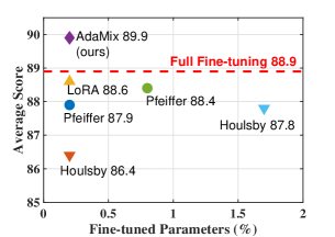
Figure 1: Performance of different parameter-efficient fine-tuning methods on GLUE development set with RoBERTa-large encoder following a setup similar to Houlsby et al. (2019) for fair comparison. We report the performance of Pfeiffer Pfeiffer et al. (2021), Houlsby Houlsby et al. (2019) and LoRA Hu et al. (2021) with their default number of fine-tuned parameters as well as the number of fine-tuned parameters used in AdaMix with a mixture of adaptations . Red dash shows the performance of full model fine-tuning.

Standard fine-tuning of large pre-trained language models (PLMs) (Devlin et al., 2019; Liu et al., 2019; Brown et al., 2020; Raffel et al., 2019) to downstream tasks requires updating all model parameters. Given the ever-increasing size of PLMs (e.g., $175$ billion parameters for GPT-3 Brown et al. (2020) and $530$ billion parameters for MT-NLG Smith et al. (2022)), even the fine-tuning step becomes expensive as it requires storing a full copy of model weights for every task. To address these challenges, recent works have developed parameter-efficient fine-tuning (PEFT) techniques. These approaches typically underperform standard full model fine-tuning, but significantly reduce the number of trainable parameters. There are many varieties of PEFT methods, including prefix-tuning (Li and Liang, 2021) and prompt-tuning (Lester et al., 2021) to condition frozen language models via natural language task descriptions, low dimensional projections using adapters (Houlsby et al., 2019; Pfeiffer et al., 2020, 2021) and more recently using low-rank approximation (Hu et al., 2021). Figure 1 shows the performance of some popular PEFT methods with varying number of tunable parameters. We observe a significant performance gap with respect to full model tuning where all PLM parameters are updated.

In this paper, we present AdaMix, a mixture of adaptation modules approach, and show that it outperforms SOTA PEFT methods and also full model fine-tuning while tuning only $0.1-0.2\%$ of PLM parameters.

In contrast to traditional PEFT methods that use a single adaptation module in every Transformer layer, AdaMix uses several adaptation modules that learn multiple views of the given task. In order to design this mixture of adaptations, we take inspiration from sparsely-activated mixture-of-experts (MoE) models. In traditional dense models (e.g., BERT (Devlin et al., 2019), GPT-3 (Brown et al., 2020)), all model weights are activated for every input example. MoE models induce sparsity by activating only a subset of the model weights for each incoming input.

Consider adapters (Houlsby et al., 2019), one of the most popular PEFT techniques, to illustrate our method. A feedforward layer (FFN) is introduced to down-project the hidden representation to a low dimension $d$ (also called the bottleneck dimension) followed by another up-project FFN to match the dimensionality of the next layer. Instead of using a single adapter, we introduce multiple project-up and project-down FFNs in each Transformer layer. We route input examples to one of the project-up and one of the project-down FFN’s resulting in the same amount of computational cost (FLOPs) as that of using a single adapter. For methods like LoRA Hu et al. (2021), that decomposes the gradient of pre-trained weights into low-rank matrices ($A$ and $B$), we introduce multiple low-rank decompositions and route the input examples to them similar to adapters.

We discuss different routing mechanism and show that stochastic routing yields good performance while eliminating the need for introducing any additional parameters for module selection. To alleviate training instability that may arise from the randomness in selecting different adaptation modules in different training steps, we leverage consistency regularization and the sharing of adaptation modules during stochastic routing.

The introduction of multiple adaptation modules results in an increased number of adaptation parameters. This does not increase computational cost but increases storage cost. To address this, we develop a merging mechanism to combine weights from different adaptation modules to a single module in each Transformer layer. This allows us to keep the number of adaptation parameters the same as that of a single adaptation module. Our merging mechanism is inspired by model weight averaging model soups (Wortsman et al., 2022) and multi BERTs (Sellam et al., 2022). Weight averaging of models with different random initialization has been shown to improve model performance in recent works (Matena and Raffel, 2021; Neyshabur et al., 2020; Frankle et al., 2020) that show the optimized models to lie in the same basin of error landscape. While the above works are geared towards fine-tuning independent models, we extend this idea to parameter-efficient fine-tuning with randomly initialized adaptation modules and a frozen language model.

Overall, our work makes the following contributions:

(a) We develop a new method AdaMix as a mixture of adaptations for parameter-efficient fine-tuning (PEFT) of large language models. Given any PEFT method of choice like adapters and low-rank decompositions, AdaMix improves downstream task performance over the underlying PEFT method.

(b) AdaMix is trained with stochastic routing and adaptation module merging to retain the same computational cost (e.g., FLOPs, #tunable adaptation parameters) and benefits of the underlying PEFT method. To better understand how AdaMix works, we demonstrate its strong connections to Bayesian Neural Networks and model ensembling.

(c) By tuning only $0.1-0.2\%$ of a pre-trained language model’s parameters, AdaMix is the first PEFT method to outperform full model fine-tuning methods for all NLU tasks on GLUE, and outperforms other competing methods for NLG and few-shot NLU tasks.

Practical benefits of PEFT methods. The most significant benefit of PEFT methods comes from the reduction in memory and storage usage. For a Transformer, the VRAM consumption can be significantly reduced as we do not need to keep track of optimizer states for the frozen parameters. PEFT methods also allow multiple tasks to share the same copy of the full (frozen) PLM. Hence, the storage cost for introducing a new task can be reduced by up to 444x (from 355MB to 0.8MB with RoBERTa-large encoder in our setting).

We present background on Mixture-of-Experts (MoE) and adapters in Section 2 of Appendix.

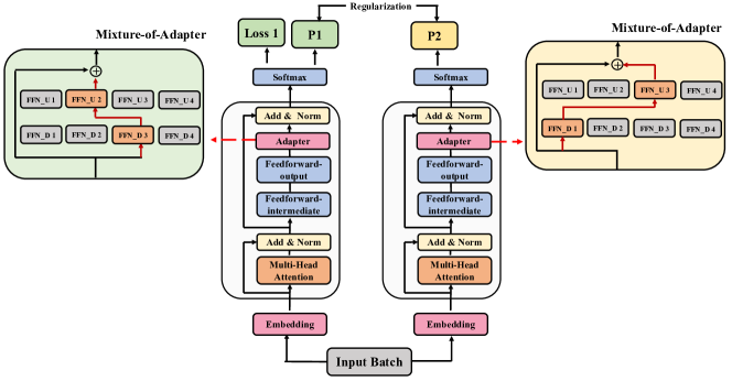
Figure 2: Mixture-of-Adaptations (AdaMix) with adapters Houlsby et al. (2019) as the underlying PEFT mechanism. For illustration, we show $M=4$ adaptation modules consisting of feedforward up (FFN_U) feedforward down ($\text{FFN\_D})$ projection matrices. The above block shown for one Transformer layer is repeated across all the layers. AdaMix stochastically routes instances from an input batch via randomly selected adaptation modules resulting in FLOPs match to a single module with consistency regularization and parameter sharing. Adaptation merging (Figure 4) collapses multiple modules to match single-module parameters in each layer.

2 Background

2.1 Mixture-of-Experts

The objective of sparsely-activated model design is to support conditional computation and increase the parameter count of neural models like Transformers while keeping the floating point operations (FLOPs) for each input example constant. Mixture-of-Experts (MoE) Transformer models (Shazeer et al., 2017; Fedus et al., 2021; Lepikhin et al., 2020; Zuo et al., 2021) achieve this by using $N$ feed-forward networks (FFN), namely “experts" denoted as $\mathbb{E}_{i=1}^{N}$, each with its own set of learnable weights that compute different representations of an input token $x$ based on context. In order to sparsify the network to keep the FLOPs constant, there is an additional gating network $\mathbb{G}$ whose output is a sparse $N$-dimensional vector to route each token via a few of these experts. Note that, a sparse model with $N=1$ corresponding to only one FFN layer in each Transformer block collapses to the traditional dense model.

Consider $x_{s}$ as the input token representation in the $s^{th}$ position to the MOE layer comprising of the $\{\mathbb{E}\}_{i=1}^{N}$ expert FFNs. Also, consider $w^{in}_{i}$ and $w^{out}_{i}$ to be the input and output projection matrices for $i^{th}$ expert. Expert output $\mathbb{E}_{i}(x_{s})$ is given by:

$$\mathbb{E}_{i}(x_{s})=w^{out}_{i}\cdot GeLU(w^{in}_{i}\cdot x_{s})$$ (1)

Consider $\mathbb{G}(x_{s})$ to be output of the gating network. Output of the sparse MoE layer is given by:

$$h(x_{s})=\sum_{i}\mathbb{G}(x_{s})_{i}\ \mathbb{E}_{i}(x_{s})$$ (2)

where $\mathbb{G}(x_{s})_{i}$ the $i^{th}$ logit of the output of $\mathbb{G}(x_{s})$ denotes the probability of selecting expert $\mathbb{E}_{i}$.

In order to keep the number of FLOPs in the sparse Transformer to be the same as that of a dense one, the gating mechanism can be constrained to route each token to only one expert FFN, i.e. $\sum_{i}\mathbb{G}_{t}(x_{s})_{i}=1$.

2.2 Adapters

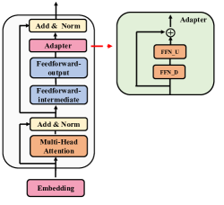
Figure 3: Conventional adapter design in standard Transformer architecture.

The predominant methodology for task adaptation is to tune all of the trainable parameters of the PLMs for every task. This raises significant resource challenges both during training and deployment. A recent study (Aghajanyan et al., 2021) shows that PLMs have a low instrinsic dimension that can match the performance of the full parameter space.

To adapt PLMs for downstream tasks with a small number of parameters, adapters (Houlsby et al., 2019) have recently been introduced as an alternative approach for lightweight tuning.

The adapter tuning strategy judiciously introduces new parameters into the original PLMs. During fine-tuning, only the adapter parameters are updated while keeping the remaining parameters of the PLM frozen. Adapters usually consist of two fully connected layers as shown in Figure 3, where the adapter layer uses a down projection $\mathcal{W}^{down}\in\mathcal{R}^{d\times r}$ to project input representation $x$ to a low dimensional space $r$ (referred as the bottleneck dimension) with $d$ being the model dimension, followed by a nonlinear activation function $f(\cdot)$, and a up-projection with $\mathcal{W}^{up}\in\mathcal{R}^{r\times d}$ to project the low-dimensional features back to the original dimension. The adapters are further surrounded by residual connections.

Given the above adapter design with parameters $\psi$, the dataset $\mathcal{D}_{K}$, a pre-trained language model encoder $enc$ with parameters $\Theta_{\mathrm{PLM}}$, where $\Theta_{\mathrm{PLM}}\gg\psi$, we want to perform the following optimization for efficient model adaptation:

$$\psi\leftarrow argmin_{\psi}\ \mathcal{L}(\mathcal{D}_{k};\Theta_{\mathrm{PLM}},\psi)$$ (3)

3 Mixture-of-Adaptations

Consider a set of $M$ adaptation modules injected in each Transformer layer, where $A_{ij}:i\in\{1\cdots L\},j\in\{1\cdots M\}$ represents the $j^{th}$ adaptation module in the $i^{th}$ Transformer layer. For illustration, we will consider adapters Houlsby et al. (2019) as the underlying parameter-efficient fine-tuning (PEFT) mechanism as a running example. Similar principles can be used for other PEFT mechanism like LoRA Hu et al. (2021) for low-rank decompositions as we show in experiments.

We adopt the popularly used Transformer architecture Vaswani et al. (2017) consisting of $L$ repeated Transformer blocks, where each block consists of a self-attention sub-layer, a fully connected feed-forward network (FFN) and residual connections around the sub-layers followed by layer normalization. Each adaptation module $A_{ij}$ corresponding to the adapters Houlsby et al. (2019) consists of a feedforward up $\mathcal{W}^{up}_{ij}$ and a feedforward down $\mathcal{W}^{down}_{ij}$ projection matrices.

3.1 Routing Policy

Recent work like THOR Zuo et al. (2021) has demonstrated stochastic routing policy like random routing to work as well as classical routing mechanism like Switch routing Fedus et al. (2021) with the following benefits. Since input examples are randomly routed to different experts, there is no requirement for additional load balancing as each expert has an equal opportunity of being activated simplifying the framework. Further, there are no added parameters, and therefore no additional computation, at the Switch layer for expert selection. The latter is particularly important in our setting for parameter-efficient fine-tuning to keep the parameters and FLOPs the same as that of a single adaptation module. To analyze the working of AdaMix, we demonstrate connections to stochastic routing and model weight averaging to Bayesian Neural Networks and model ensembling in Section 3.5.

In the stochastic routing policy for AdaMix with adapters, at any training step, we randomly select a pair of feedforward up and feedforward down projection matrices in the $i^{th}$ Transformer layer as $A_{i}=\{\mathcal{W}^{up}_{ij},\mathcal{W}^{down}_{ik}\}$ and $B_{i}=\{\mathcal{W}^{up}_{ij^{\prime}},\mathcal{W}^{down}_{ik^{\prime}}\}$ respectively. Given this selection of adaptation modules $A_{i}$ and $B_{i}$ in each Transformer layer in every step, all the inputs in a given batch are processed through the same set of modules. Given an input representation $x$ in a given Transformer layer, the above pair of modules perform the following transformations:

$$x\leftarrow x+f(x\cdot\mathcal{W}^{down})\cdot\mathcal{W}^{up}$$ (4)

Such stochastic routing enables adaptation modules to learn different transformations during training and obtain multiple views of the task. However, this also creates a challenge on which modules to use during inference due to random routing protocol during training. We address this challenge with the following two techniques that further allow us to collapse adaptation modules and obtain the same computational cost (FLOPs, #tunable adaptation parameters) as that of a single module.

3.2 Consistency regularization

Consider $\mathcal{A}=\{A_{i=1}^{L}\}$ and $\mathcal{B}=\{B_{i=1}^{L}\}$ to be the sets of adaptation modules (e.g., projection matrices) activated during two stochastic forward passes through the network for an input $x$ across $L$ layers of the Transformer. The objective of consistency regularization is to enable the adaptation modules to share information and prevent divergence. To this end, we add the following consistency loss as a regularizer to the task-specific optimization loss:

$$\mathcal{L}=-\bigg{(}\sum_{c=1}^{C}\mathcal{I}(x,c)\ \log\text{softmax}(z_{c}^{\mathcal{A}}(x))+\\ \frac{1}{2}\big{(}\mathcal{KL}(z_{(.)}^{\mathcal{A}}(x)||z_{(.)}^{\mathcal{B}}(x))+\mathcal{KL}(z_{(.)}^{\mathcal{B}}(x)||z_{(.)}^{\mathcal{A}}(x))\bigg{)}$$ (5)

where $\mathcal{I}(x,c)$ is a binary indicator ($0$ or $1$) if class label $c$ is the correct classification for $x$ and $z_{(.)}^{\mathcal{A}}(x)$ and $z_{(.)}^{\mathcal{B}}(x)$ are the predicted logits while routing through two sets of adaptation modules $\mathcal{A}$ and $\mathcal{B}$ respectively with $\mathcal{KL}$ denoting the Kullback-Leibler divergence. $x$ is the input representation from the PLM with frozen parameters and only the parameters of modules $\{\mathcal{W}^{up},\mathcal{W}^{down}\}$ are updated during training.

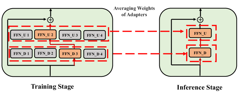
Figure 4: Stochastic routing during training activates different adaptation modules to have multiple views of the task with FLOPs match to a single module. Merging weights of the adaptation modules ($\{\text{FFN}\_\text{U}_{i}\},\{\text{FFN}\_\text{D}_{i}\}:i\in\{1\cdots 4\}$) by averaging preserves improved performance with parameter match to a single-module.

3.3 Adaptation module merging

While the above regularization mitigates inconsistency in random module selection during inference, it still results in increased serving cost to host several adaptation modules. Prior works in fine-tuning language models for downstream tasks have shown improved performance on averaging the weights of different models fine-tuned with different random seeds outperforming a single fine-tuned model. Recent work Wortsman et al. (2022) has also shown that differently fine-tuned models from the same initialization lie in the same error basin motivating the use of weight aggregation for robust task summarization. We adopt and extend prior techniques for language model fine-tuning to our parameter-efficient training of multi-view adaptation modules.

In contrast to the aforementioned techniques like stochastic routing and consistency regularization that are applied at the training phase, we employ adaptation merging only during inference. Given a set of adaptation modules, $\mathcal{W}^{up}_{ij}$ and $\mathcal{W}^{down}_{ik}$ for $i\in\{1\cdots L\}$ and $\{j,k\}\in\{1\cdots M\}$, we simply average the weights of all the corresponding modules (e.g., project-up or project-down matrices) in every Transformer layer to collapse to a single module $\{\mathcal{W^{\prime}}^{up}_{i},\mathcal{W^{\prime}}^{down}_{i}\}$, where:

$$\mathcal{W^{\prime}}^{up}_{i}\leftarrow\frac{1}{M}\sum_{j=1}^{M}\mathcal{W}^{up}_{ij}\qquad\mathcal{W^{\prime}}^{down}_{i}\leftarrow\frac{1}{M}\sum_{j=1}^{M}\mathcal{W}^{down}_{ij}$$ (6)

3.4 Adaptation module sharing

While stochastic routing to multi-view adaptation modules increases the model capacity, it can also impact downstream tasks with less amounts of labeled data for tuning several sets of adaptation modules. To address this challenge, we use another mechanism to share some of the adaption modules (e.g., project-down or the project-up operations) to improve training efficiency. In the standard setting for adapters, we share only the feedforward projection-up matrices i.e., $\mathcal{W}^{up}_{ij}=\mathcal{W}^{up}_{i}$. We investigate these design choices via ablation studies in our experiments in Section 4.3 and Section B in Appendix.

3.5 Connection to Bayesian Neural Networks and Model Ensembling

Bayesian Neural Network (BNN) (Gal and Ghahramani, 2015) replaces a deterministic model’s weight parameters by a distribution over the parameters. For inference, BNN averages over all the possible weights, also referred to as marginalization. Consider $f^{\mathcal{W}(x)}\in\mathbb{R}^{d}$ to be the $d-$dimensional output of such a neural network where the model likelihood is given by $p(y|f^{\mathcal{W}(x)})$. In our setting, $\mathcal{W}=\langle\mathcal{W}^{up},\mathcal{W}^{down}\rangle$ along with frozen PLM parameters that are dropped from the notation for simplicity. For classification, we can further apply a softmax likelihood to the output to obtain: $P(y=c|x,W)=softmax(f^{\mathcal{W}(x)})$. Given an instance $x$, the probability distribution over the classes is given by marginalization over the posterior distribution as: $p(y=c|x)=\int_{\mathcal{W}}p(y=c|f^{\mathcal{W}(x)})p(\mathcal{W}|X,Y)d\mathcal{W}$.

This requires averaging over all possible model weights, which is intractable in practice. Therefore, several approximation methods have been developed based on variational inference methods and stochastic regularization techniques using dropouts. In this work, we leverage another stochastic regularization in the form of random routing. Here, the objective is to find a surrogate distribution $q_{\theta}(w)$ in a tractable family of distributions that can replace the true model posterior that is hard to compute. The ideal surrogate is identified by minimizing the Kullback-Leibler (KL) divergence between the candidate and the true posterior.

Consider $q_{\theta}(\mathcal{W})$ to be the stochastic routing policy which samples $T$ masked model weights $\{\widetilde{\mathcal{W}_{t}}\}_{t=1}^{T}\sim q_{\theta}(\mathcal{W})$. For classification tasks, the approximate posterior can be now obtained by Monte-Carlo integration Gal et al. (2017) as:

$$\begin{split}p(y=c|x)&\approx p(y=c|f^{\mathcal{W}}(x))q_{\theta}(\mathcal{W})d\mathcal{W}\\ &\approx\frac{1}{T}\ \sum_{t=1}^{T}p(y=c|f^{\widetilde{\mathcal{W}_{t}}}(x))\\ &=\frac{1}{T}\ \sum_{t=1}^{T}softmax(f^{\widetilde{\mathcal{W}_{t}}}(x))\end{split}$$ (7)

However, computing the approximate posterior above in our setting requires storing all the stochastic model weights $\mathcal{W}_{t}(x)$ which increases the serving cost during inference. To reduce this cost, we resort to the other technique for weight averaging via adaptation module merging during inference.

Let $\mathcal{L}^{AM}_{\mathcal{W}}=\mathbb{E}_{x,y}\mathcal{L}(softmax(f^{\widetilde{\mathcal{W}}}(x),y)$ denote the expected loss with merging of the stochastic adaptation weights with $\widetilde{\mathcal{W}}=\frac{1}{T}\sum_{t}\widetilde{\mathcal{W}_{t}}$ (from Equation 6) and $\mathcal{L}$ denoting the cross-entropy loss. Consider $\mathcal{L}^{Ens}_{\mathcal{W}}=\mathbb{E}_{x,y}\mathcal{L}(\frac{1}{T}\ \sum_{t=1}^{T}softmax(f^{\widetilde{\mathcal{W}_{t}}}(x),y))$ denote the expected loss from logit-level stochastic model ensembling (from Equation 7).

Prior work (Wortsman et al., 2022) shows that averaging the weights of multiple models fine-tuned with different hyper-parameters improves model performance. They analytically show the similarity in loss between weight-averaging ($\mathcal{L}^{AM}_{\mathcal{W}}$ in our setting) and logit-ensembling ($\mathcal{L}^{Ens}_{\mathcal{W}}$ in our setting) as a function of the flatness of the loss and confidence of the predictions. While the above analysis is geared towards averaging of multiple independently fine-tuned model weights, we can apply a similar analysis in our setting towards averaging of multiple stochastically obtained adaptation weights in obtaining a favorable loss $\mathcal{L}^{AM}_{\mathcal{W}}$. Further, adaptation merging reduces the serving cost during inference since we need to retain only one copy of the merged weights as opposed to logit-ensembling which requires copies of all the adaptation weights.

Model	#Param.	MNLI	QNLI	SST2	QQP	MRPC	CoLA	RTE	STS-B	Avg.
		Acc	Acc	Acc	Acc	Acc	Mcc	Acc	Pearson
Full Fine-tuning†	355.0M	90.2	94.7	96.4	92.2	90.9	68.0	86.6	92.4	88.9
Pfeiffer Adapter†	3.0M	90.2	94.8	96.1	91.9	90.2	68.3	83.8	92.1	88.4
Pfeiffer Adapter†	0.8M	90.5	94.8	96.6	91.7	89.7	67.8	80.1	91.9	87.9
Houlsby Adapter†	6.0M	89.9	94.7	96.2	92.1	88.7	66.5	83.4	91.0	87.8
Houlsby Adapter†	0.8M	90.3	94.7	96.3	91.5	87.7	66.3	72.9	91.5	86.4
LoRA†	0.8M	90.6	94.8	96.2	91.6	90.2	68.2	85.2	92.3	88.6
AdaMix Adapter	0.8M	90.9	95.4	97.1	92.3	91.9	70.2	89.2	92.4	89.9

Table 1: Results for NLU tasks on GLUE development set with RoBERTa-large encoder. The best result on each task is in bold and “-” denotes missing measure. AdaMix with a mixture of adapters outperforms all competing methods as well as fully fine-tuned large model with only $0.23\%$ tunable parameters.^† denotes results reported from Hu et al. (2021). Mcc refers to Matthews correlation coefficient, and Pearson refers to Pearson correlation. #Param. denotes the number of tunable adaptation parameters used during inference.

4 Experiments

4.1 Experimental Setup

Dataset. We perform experiments on a wide range of tasks including eight natural language understanding (NLU) tasks in the General Language Understanding Evaluation (GLUE) benchmark Wang et al. (2019) and three natural language generation (NLG) tasks, namely, E2E Novikova et al. (2017), WebNLG Gardent et al. (2017) and DART Nan et al. (2020). For the NLU and NLG tasks, we follow the same setup as Houlsby et al. (2019) and Li and Liang (2021); Hu et al. (2021), respectively.

Baselines. We compare AdaMix to full model fine-tuning and several state-of-the-art parameter-efficient fine-tuning (PEFT) methods, namely, Pfeiffer Adapter Pfeiffer et al. (2021), Houlsby Adapter Houlsby et al. (2019), BitFit Zaken et al. (2021), Prefix-tuning Li and Liang (2021), UNIPELT Mao et al. (2021) and LoRA Hu et al. (2021). We use BERT-base Devlin et al. (2019) and RoBERTa-large Liu et al. (2019) as encoders for NLU tasks (results in Table 1 and Table 2), and GPT-2 Brown et al. (2020) for NLG tasks (results in Table 3).

AdaMix implementation details. We implement AdaMix in Pytorch and use Tesla V100 gpus for experiments with detailed hyper-parameter configurations presented in Section D in Appendix. AdaMix with adapters uses a dimension of $16$ and $48$ using BERT-base and RoBERTa-large encoders following the setup of Hu et al. (2021); Mao et al. (2021) for fair comparison. AdaMix with LoRA uses rank $r=4$ following the setup of Hu et al. (2021) to keep the same number of adaptation parameters during inference. The number of adaptation modules in AdaMix is set to $4$ for all the tasks and encoders unless otherwise specified. The impact of adapter dimension and number of adaptation modules for NLU tasks are investigated in Table 9 and 10. For most of the experiments and ablation analysis, we report results from AdaMix with adapters for NLU tasks. For demonstrating the generalizability of our framework, we report results from AdaMix with LoRA Hu et al. (2021) as the underlying PEFT mechanism for NLG tasks.

4.2 Key Results

4.2.1 NLU Tasks

Tables 1 and 2 show the performance comparison among PEFT models with RoBERTa-large and BERT-base encoders respectively. Fully fine-tuned RoBERTa-large and BERT-base provide the ceiling performance. We observe AdaMix with a mixture-of-adapters to significantly outperform other state-of-the-art baselines on most tasks with different encoders. AdaMix with adapters is the only PEFT method which outperforms full model fine-tuning on all the tasks and on average score.

Model	#Param.	Avg.
Full Fine-tuning†	110M	82.7
Houlsby Adapter†	0.9M	83.0
BitFit⋄	0.1M	82.3
Prefix-tuning†	0.2M	82.1
LoRA†	0.3M	82.2
UNIPELT (AP)†	1.1M	83.1
UNIPELT (APL)†	1.4M	83.5
AdaMix Adapter	0.9M	84.5

Table 2: Results for NLU tasks on GLUE development set with BERT-base encoder and AdaMix with a mixture-of-adapters. The best result on each task is in bold. ^† and ^⋄ denote results reported from Mao et al. (2021); Zaken et al. (2021). Detailed task-specific results are reported in Table 13 of Appendix. #Param. refers to the number of tunable adaptation parameters during inference.

4.2.2 NLG Tasks

Model	#Param.	BLEU	NIST	MET	ROUGE-L	CIDEr
Full Fine-tuning†	354.92M	68.2	8.62	46.2	71.0	2.47
Lin AdapterL†	0.37M	66.3	8.41	45.0	69.8	2.40
Lin Adapter†	11.09M	68.9	8.71	46.1	71.3	2.47
Houlsby Adapter†	11.09M	67.3	8.50	46.0	70.7	2.44
FT${}^{Top2^{\dagger}{}}$	25.19M	68.1	8.59	46.0	70.8	2.41
PreLayer†	0.35M	69.7	8.81	46.1	71.4	2.49
LoRA†	0.35M	70.4	8.85	46.8	71.8	2.53
LoRA (repr.)	0.35M	69.8	8.77	46.6	71.8	2.52
AdaMix Adapter	0.42M	69.8	8.75	46.8	71.9	2.52
AdaMix LoRA	0.35M	71.0	8.89	46.8	72.2	2.54

Table 3: Results on E2E NLG Challenge with GPT-2 medium backbone. Best result on each task is in bold. We report AdaMix results with both adapters and LoRA as underlying PEFT method. AdaMix outperforms all competing methods as well as fully fine-tuned large model with only $0.1\%$ tunable parameters.^† denotes results reported from Hu et al. (2021) and repr. denotes reproduced results. #Param. denotes the number of tunable adaptation parameters used during inference. Results on DART and WebNLG presented in Tables 4 and 5 in Appendix.

AdaMix leverages mixture of adaptations to improve over underlying PEFT method as demonstrated in Table 3 for E2E NLG i.e. AdaMix with LoRA and AdaMix with adapters outperform LoRA Hu et al. (2021) and adapters Houlsby et al. (2019) respectively. We report results on DART and WebNLG in Tables 4 and 5 in Appendix.

Model	#Param.	BLEU
Full Fine-tuning†	354.92M	46.2
Lin AdapterL†	0.37M	42.4
Lin Adapter†	11.09M	45.2
FT${}^{Top2^{\dagger}{}}$	25.19M	41.0
PrefLayer†	0.35M	46.4
LoRA†	0.35M	47.1
LoRA (repr.)	0.35M	47.35
AdaMix Adapter	0.42M	47.72
AdaMix LoRA	0.35M	47.86

Table 4: Results on DART with GPT-2 backbone encoder. Best result on each task is in bold. We report AdaMix results with both adapters and LoRA as underlying PEFT method. AdaMix outperforms all competing methods as well as fully fine-tuned large model with only $0.1\%$ tunable parameters.^† denotes results reported from Hu et al. (2021) and repr. denotes reproduced results. #Param. denotes the number of tunable adaptation parameters used during inference.

Model	#Param.	BLEU
Full Fine-tuning†	354.92M	46.5
Lin AdapterL†	0.37M	50.2
Lin Adapter†	11.09M	54.9
FT${}^{Top2^{\dagger}{}}$	25.19M	36.0
Prefix†	0.35M	55.1
LoRA†	0.35M	55.3
LoRA (repr.)	0.35M	55.37
AdaMix Adapter	0.42M	54.94
AdaMix LoRA	0.35M	55.64

Table 5: Results on WebNLG with GPT-2 medium backbone. The results are based on all categories in the test set of WebNLG. Best result on each task is in bold. We report AdaMix results with both adapters and LoRA as underlying PEFT method. AdaMix outperforms all competing methods as well as fully fine-tuned large model with only $0.1\%$ tunable parameters.^† denotes results reported from Hu et al. (2021) and repr. denotes reproduced results. #Param. denotes the number of tunable adaptation parameters used during inference.

4.2.3 Few-shot NLU

In contrast to the fully supervised setting in the above experiments, we also perform few-shot experiments on six GLUE tasks following the same setup (e.g., shots, train and test splits) and evaluation as in Wang et al. (2021). Detailed experimental configuration presented in Section A of Appendix. AdaMix uses a mixture-of-adapters with prompt-based fine-tuning Gao et al. (2021).

Model	MNLI	RTE	QQP	SST2	Subj	MPQA	Avg.
Full Prompt Fine-tuning*	62.8 (2.6)	66.1 (2.2)	71.1 (1.5)	91.5 (1.0)	91.0 (0.5)	82.7 (3.8)	77.5
Head-only*	54.1 (1.1)	58.8 (2.6)	56.7 (4.5)	85.6 (1.0)	82.1 (2.5)	64.1 (2.1)	66.9
BitFit*	54.4 (1.3)	59.8 (3.5)	58.6 (4.4)	87.3 (1.1)	83.9 (2.3)	65.8 (1.8)	68.3
Prompt-tuning*	47.3 (0.2)	53.0 (0.6)	39.9 (0.7)	75.7 (1.7)	51.5 (1.4)	70.9 (2.4)	56.4
Houlsby Adapter*	35.7 (1.1)	51.0 (3.0)	62.8 (3.0)	57.0 (6.2)	83.2 (5.4)	57.2 (3.5)	57.8
LiST Adapter*	62.4 (1.7)	66.6 (3.9)	71.2 (2.6)	91.7 (1.0)	90.9 (1.3)	82.6 (2.0)	77.6
AdaMix Adapter	65.6 (2.6)	69.6 (3.4)	72.6 (1.2)	91.8 (1.1)	91.5 (2.0)	84.7 (1.6)	79.3

Table 6: Average performance and standard deviation of several parameter-efficient fine-tuning strategies based on RoBERTa-large with $|\mathcal{K}|=30$ training labels. The best performance is shown in bold. Prompt-tuning, Head-only and BitFit tune $1M$ model parameters during inference. Houlsby Adapter, LiST Adapter and AdaMix Adapter tune $14M$ model parameters. ^* denotes that the results are taken from Wang et al. (2021).

Table 6 shows the performance comparison among different PEFT methods with $|K|=30$ labeled examples with RoBERTa-large as frozen encoder. We observe significant performance gap for most PEFT methods with full model prompt-based fine-tuning i.e. with all model parameters being updated. AdaMix with adapters outperforms full model tuning performance for few-shot NLU similar to that in the fully supervised setting. Note that AdaMix and LiST Wang et al. (2021) use similar adapter design with prompt-based fine-tuning.

4.3 Ablation Study

We perform all the ablation analysis on AdaMix with adapters for parameter-efficient fine-tuning.

Analysis of adaptation merging. In this ablation study, we do not merge adaptation modules and consider two different routing strategies at inference time: (a) randomly routing input to any adaptation module, and (b) fixed routing where we route all the input to the first adaptation module in AdaMix. From Table 7, we observe AdaMix with adaptation merging to perform better than any of the other variants without the merging mechanism. Notably, all of the AdaMix variants outperform full model tuning.

Model	#Param.	Avg.
Full Fine-tuning	110M	82.7
AdaMix w/ Merging	0.9M	84.5
AdaMix w/o Merging + RandomRouting	3.6M	83.3
AdaMix w/o Merging + FixedRouting	0.9M	83.7
AdaMix w/o Merging + Ensemble	3.6M	83.2

Table 7: AdaMix without adaptation merging and different routing and ensembling strategies. Average results are presented on GLUE development set with BERT-base encoder. Detailed task results in Table 14 of Appendix for BERT-base and RoBERTa-large encoders.

Moreover, Figure 5 shows that the performance of merging mechanism is consistently better than the average performance of random routing and comparable to the best performance of random routing.

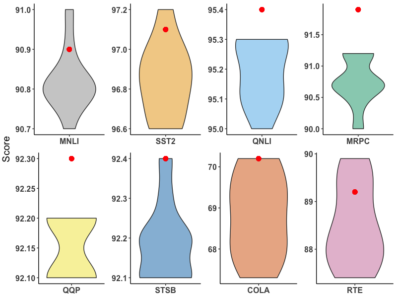
Figure 5: Violin plot of AdaMix-RandomRouting performance distribution with RoBERTa-large encoders. Red dot denotes the performance of AdaMix.

Averaging weights v.s. ensembling logits. We compare AdaMix with a variant of logit ensembling, denoted as AdaMix-Ensemble. To this end, we make four random routing passes through the network for every input ($T$=$4$) and average the logits from different passes as the final predicted logit. Inference time for this ensembling method is 4 $\times$ AdaMix. We run repeated experiments with three different seeds and report mean performance in Table 7. We observe AdaMix with adaptation weight averaging to outperform logit-ensembling following our analysis ($\mathcal{L}^{AM}_{\mathcal{W}}$ v.s. $\mathcal{L}^{Ens}_{\mathcal{W}}$) in Section 3.5.

Analysis of consistency regularization. We drop consistency regularization during training for ablation and demonstrate significant performance degradation in Table 8.

Model/# Train	MNLI	QNLI	SST2	MRPC	RTE
	393k	108k	67k	3.7k	2.5k
Full Fine-tuning	90.2	94.7	96.4	90.9	86.6
AdaMix	90.9	95.4	97.1	91.9	89.2
w/o Consistency	90.7	95.0	97.1	91.4	84.8
w/o Sharing	90.9	95.0	96.4	90.4	84.1

Table 8: Ablation study demonstrating the impact of consistency regularization and sharing in AdaMix.

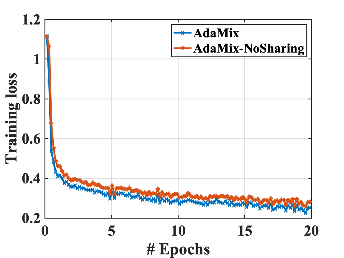
(a) MNLI

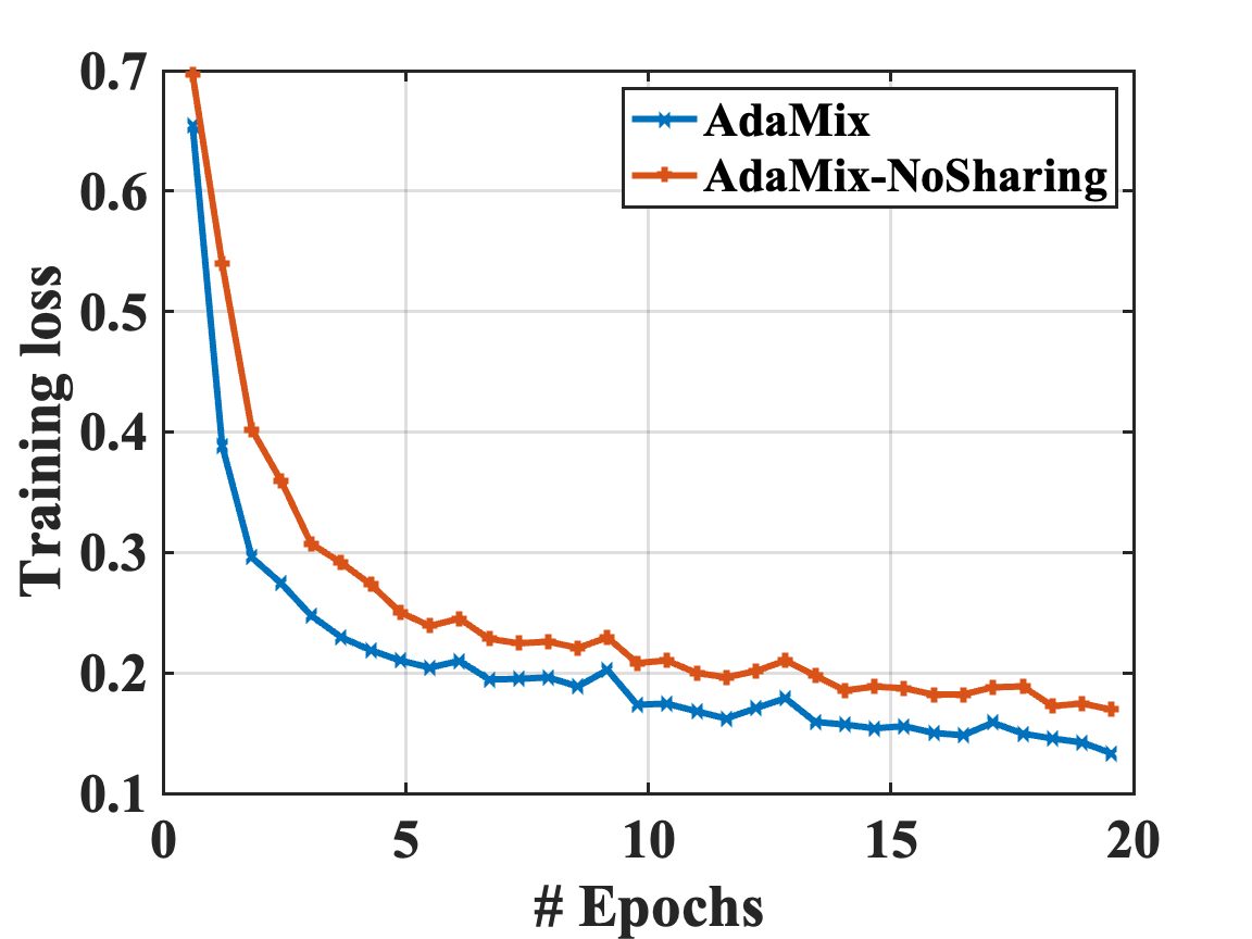
(b) QNLI

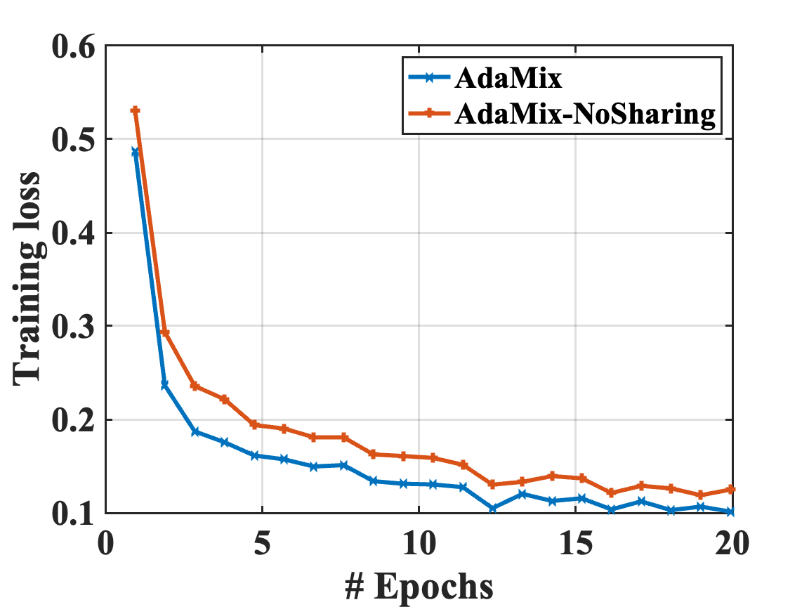
(c) SST2

Figure 7: Convergence analysis demonstrating the impact of adapter sharing design in AdaMix.

Analysis of adaptation module sharing. We remove adaptation module sharing in AdaMix for ablation and keep four different copies of project-down and four project-up FFN layers. From Table 8 we observe the performance gap between AdaMix and AdaMix w/o sharing to increase with decrease in the dataset size demonstrating the importance of parameter sharing for low-resource tasks (e.g., RTE, MRPC). This is further demonstrated in Figure 7 in Appendix which shows a faster convergence and lower training loss of AdaMix with sharing compared to that without given the same number of training steps. We explore which adaptation module to share (project-up v.s. project-down) in Table 11 in Appendix that depict similar results.

Impact of the number of adaptation modules. In this study, we vary the number of adaptation modules in AdaMix as $2$, $4$ and $8$ during training. Table 9 shows diminishing returns on aggregate task performance with increasing number of modules. As we increase sparsity and the number of tunable parameters by increasing the number of adaptation modules, low-resource tasks like RTE and SST-2 – with limited amount of labeled data for fine-tuning – degrade in performance compared to high-resource tasks like MNLI and QNLI.

Adaptation	MNLI	QNLI	SST2	MRPC	RTE
Module	393k	108k	67k	3.7k	2.5k
2	90.9	95.2	96.8	90.9	87.4
4*	90.9	95.4	97.1	91.9	89.2
8	90.9	95.3	96.9	91.4	87.4

Table 9: Varying the number of adaptation modules in AdaMix with RoBERTa-large encoder. ^* denotes the number of modules used in AdaMix with adapters.

Impact of adapter bottleneck dimension. Table 10 shows the impact of bottleneck dimension of adapters with different encoders in AdaMix. The model performance improves with increase in the number of trainable parameters by increasing the bottleneck dimension with diminishing returns after a certain point.

Adapter	#Param.	MNLI	QNLI	SST2	MRPC	RTE
Dimension		393k	108k	67k	3.7k	2.5k
8	0.4M	90.7	95.2	96.8	91.2	87.7
16*	0.8M	90.9	95.4	97.1	91.9	89.2
32	1.5M	91.0	95.4	96.8	90.7	89.2

Table 10: Varying the bottleneck dimension of adapters in AdaMix with RoBERTa-large encoder. ^* denotes the bottleneck dimension used in AdaMix with adapters. Results with BERT-base encoder in Table 12 in Appendix.

5 Related Work

Parameter-efficient fine-tuning of PLMs. Recent works on parameter-efficient fine-tuning (PEFT) can be roughly categorized into two categories: (1) tuning a subset of existing parameters including head fine-tuning Lee et al. (2019), bias term tuning Zaken et al. (2021), (2) tuning newly-introduced parameters including adapters Houlsby et al. (2019); Pfeiffer et al. (2020), prompt-tuning Lester et al. (2021), prefix-tuning Li and Liang (2021) and low-rank adaptation Hu et al. (2021). As opposed to prior works operating on a single adaptation module, AdaMix introduces a mixture of adaptation modules with stochastic routing during training and adaptation module merging during inference to keep the same computational cost as with a single module. Further, AdaMix can be used on top of any PEFT method to further boost its performance.

Mixture-of-Expert (MoE).  Shazeer et al., 2017 introduced the MoE model with a single gating network with $Top$-$k$ routing and load balancing across experts. Fedus et al., 2021 propose initialization and training schemes for $Top$-$1$ routing. Zuo et al., 2021 propose consistency regularization for random routing; Yang et al., 2021 propose $k$ $Top$-$1$ routing with expert-prototypes, and Roller et al., 2021; Lewis et al., 2021 address other load balancing issues. All the above works study sparse MoE with pre-training the entire model from scratch. In contrast, we study parameter-efficient adaptation of pre-trained language models by tuning only a very small number of sparse adapter parameters.

Averaging model weights. Recent explorations Szegedy et al. (2016); Matena and Raffel (2021); Wortsman et al. (2022); Izmailov et al. (2018) study model aggregation by averaging all the model weights. Matena and Raffel (2021) propose to merge pre-trained language models which are fine-tuned on various text classification tasks. Wortsman et al. (2022) explores averaging model weights from various independent runs on the same task with different hyper-parameter configurations. In contrast to the above works on full model fine-tuning, we focus on parameter-efficient fine-tuning. We explore weight averaging for merging weights of adaptation modules consisting of small tunable parameters that are updated during model tuning while keeping the large model parameters fixed.

6 Conclusions

We develop a new framework AdaMix for parameter-efficient fine-tuning (PEFT) of large pre-trained language models (PLM). AdaMix leverages a mixture of adaptation modules to improve downstream task performance without increasing the computational cost (e.g., FLOPs, parameters) of the underlying adaptation method. We demonstrate AdaMix to work with and improve over different PEFT methods like adapters and low rank decompositions across NLU and NLG tasks.

By tuning only $0.1-0.2\%$ of PLM parameters, AdaMix outperforms full model fine-tuning that updates all the model parameters as well as other state-of-the-art PEFT methods.

7 Limitations

The proposed AdaMix method is somewhat compute-intensive as it involves fine-tuning large-scale language models. The training cost of the proposed AdaMix is higher than standard PEFT methods since the training procedure involves multiple copies of adapters. Based on our empirical observation, the number of training iterations for AdaMix is usually between 1$\sim$2 times the training for standard PEFT methods. This imposes negative impact on carbon footprint from training the described models.

AdaMix is orthogonal to most of the existing parameter-efficient fine-tuning (PEFT) studies and is able to potentially improve the performance of any PEFT method. In this work, we explore two representative PEFT methods like adapter and LoRA but we did not experiment with other combinations like prompt-tuning and prefix-tuning. We leave those studies to future work.

8 Acknowledgment

The authors would like to thank the anonymous referees for their valuable comments and helpful suggestions and would like to thank Guoqing Zheng and Ruya Kang for their insightful comments on the project. This work is supported in part by the US National Science Foundation under grants NSF-IIS 1747614 and NSF-IIS-2141037. Any opinions, findings, and conclusions or recommendations expressed in this material are those of the author(s) and do not necessarily reflect the views of the National Science Foundation.

Appendix

Appendix A Few-shot NLU Datasets

Data. In contrast to the fully supervised setting in the above experiments, we also perform few-shot experiments following the prior study Wang et al. (2021) on six tasks including MNLI Williams et al. (2018), RTE (Dagan et al., 2005; Bar Haim et al., 2006; Giampiccolo et al., 2007; Bentivogli et al., 2009), QQP and SST-2 (Socher et al., ). The results are reported on their development set following (Zhang et al., 2021). MPQA (Wiebe et al., 2005) and Subj (Pang and Lee, 2004) are used for polarity and subjectivity detection, where we follow Gao et al. (2021) to keep $2,000$ examples for testing. The few-shot model only has access to $|\mathcal{K}|$ labeled samples for any task. Following true few-shot learning setting (Perez et al., 2021; Wang et al., 2021), we do not use any additional validation set for any hyper-parameter tuning or early stopping. The performance of each model is reported after fixed number of training epochs. For a fair comparison, we use the same set of few-shot labeled instances for training as in Wang et al. (2021). We train each model with $5$ different seeds and report average performance with standard deviation across the runs. In the few-shot experiments, we follow Wang et al. (2021) to train AdaMix via the prompt-based fine-tuning strategy. In contrast to Wang et al. (2021), we do not use any unlabeled data.

Appendix B Ablation Study

Model	MNLI	SST2
	Acc	Acc
Sharing Project-up	90.9	97.1
Sharing Project-down	90.8	97.1

Table 11: Ablation study demonstrating the impact of parameter sharing in AdaMix adapter framework.

Adapter Dim	#Param.	MNLI	QNLI	SST2	MRPC	RTE
		393k	108k	67k	3.7k	2.5k
BERTBASE
8	0.1M	82.2	91.1	92.2	87.3	72.6
16	0.3M	83.0	91.5	92.2	88.2	72.9
32	0.6M	83.6	91.3	92.2	88.5	73.6
48*	0.9M	84.7	91.5	92.4	89.5	74.7
64	1.2M	84.4	91.8	92.3	88.2	75.1
RoBERTaLARGE
8	0.4M	90.7	95.2	96.8	91.2	87.7
16*	0.8M	90.9	95.4	97.1	91.9	89.2
32	1.5M	91.0	95.4	96.8	90.7	89.2

Table 12: Varying the bottleneck dimension of adapters in AdaMix with BERT-base and RoBERTa-large encoder. ^* denotes the bottleneck dimension used in AdaMix with adapters.

Appendix C Detailed Results on NLU Tasks

The results on NLU tasks are included in Table 1 and Table 13. The performance AdaMix with RoBERTa-large encoder achieves the best performance in terms of different task metrics in the GLUE benchmark. AdaMix with adapters is the only PEFT method which outperforms full model fine-tuning on all the tasks and on average score. Additionally, the improvement brought by AdaMix is more significant with BERT-base as the encoder, demonstrating 2.2% and 1.2% improvement over the performance of full model fine-tuning and the best performing baseline UNIPELT with BERT-base. The improvement is observed to be consistent as that with RoBERTa-large on every task. The NLG results are included in Table 4 and 5.

Model	#Param.	MNLI	QNLI	SST2	QQP	MRPC	CoLA	RTE	STS-B	Avg.
		Acc	Acc	Acc	Acc /F1	Acc/F1	Mcc	Acc	Pearson
Full Fine-tuning†	110M	83.2	90.0	91.6	-/87.4	-/90.9	62.1	66.4	89.8	82.7
Houlsby Adapter†	0.9M	83.1	90.6	91.9	-/86.8	-/89.9	61.5	71.8	88.6	83.0
BitFit⋄	0.1M	81.4	90.2	92.1	-/84.0	-/90.4	58.8	72.3	89.2	82.3
Prefix-tuning†	0.2M	81.2	90.4	90.9	-/83.3	-/91.3	55.4	76.9	87.2	82.1
LoRA†	0.3M	82.5	89.9	91.5	-/86.0	-/90.0	60.5	71.5	85.7	82.2
UNIPELT (AP)†	1.1M	83.4	90.8	91.9	-/86.7	-/90.3	61.2	71.8	88.9	83.1
UNIPELT (APL)†	1.4M	83.9	90.5	91.5	85.5	-/90.2	58.6	73.7	88.9	83.5
AdaMix Adapter	0.9M	84.7	91.5	92.4	90.7/	89.5/	62.9	74.7	89.9	84.5
	0.9M				87.6	92.4

Table 13: Main results on GLUE development set with BERT-base encoder. The best result on each task is in bold and “-” denotes the missing measure. ^† and ^⋄ denote that the reported results are taken from Mao et al. (2021); Zaken et al. (2021). The average performance is calculated based on F1 of QQP and MRPC. #Param. refers to the number of updated parameters in the inference stage.

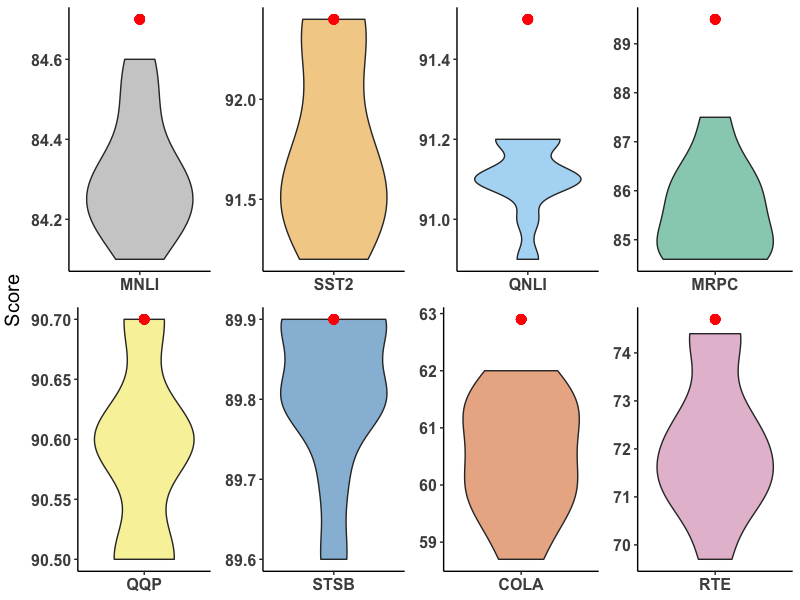
(a) BERT-base

(b) RoBERTa-large

Figure 6: Violin plot of AdaMix-RandomRouting performance distribution with BERT-base and RoBERTa-large encoders. Red dot denotes the performance of AdaMix.

Model	#Param.	MNLI	QNLI	SST2	QQP	MRPC	CoLA	RTE	STS-B	Avg.
		Acc	Acc	Acc	Acc /F1	Acc/F1	Mcc	Acc	Pearson
BERTBASE
Full Fine-tuning	110M	83.2	90.0	91.6	-/87.4	-/90.9	62.1	66.4	89.8	82.7
AdaMix	0.9M	84.7	91.5	92.4	90.7/	89.5/	62.9	74.7	89.9	84.5
					87.6	92.4
AdaMix-RandomRouting	3.6M	84.3	91.1	91.8	90.6/	85.6/	60.5	72.1	89.8	83.3
					87.4	89.1
AdaMix-FixedRouting	0.9M	84.5	91.1	91.6	90.5/	87.5/	61.4	73.3	89.8	83.7
					87.3	90.8
AdaMix-Ensemble	3.6M	84.3	91.2	91.6	90.5/	85.9/	59.4	72.1	89.8	83.2
					87.4	89.4
RoBERTaLARGE
Full Fine-tuning	355.0M	90.2	94.7	96.4	92.2/-	90.9/-	68.0	86.6	92.4	88.9
AdaMix	0.8M	90.9	95.4	97.1	92.3/	91.9/	70.2	89.2	92.4	89.9
					89.8	94.1
AdaMix-RandomRouting	3.2M	90.8	95.2	96.8	92.2/	90.8/	68.8	88.5	92.2	89.4
					89.6	93.3
AdaMix-FixedRouting	0.8M	90.7	95.1	96.8	92.1/	91.2/	68.6	89.2	92.2	89.5
					89.5	93.6
AdaMix-Ensemble	3.2M	90.9	95.3	97.0	92.2/	91.0/	69.3	89.1	92.4	89.7
					89.7	93.5

Table 14: Comparing the impact of different routing and ensembling strategies with AdaMix. Results are presented on GLUE development set with BERT-base and RoBERTa-large encoders. Average results are calculated following Table 1 and Table 2 for consistency. The best result on each task is in bold and “-” denotes the missing measure.

Appendix D Hyper-parameter

Detailed hyper-parameter configuration for different tasks presented in Table 15 and Table 16.

Task	Learning rate	epoch	batch size	warmup	weight decay	adapter size	adapter num
BERTBASE
MRPC	4e$-4$	100	16	0.06	0.1	48	4
CoLA	5e$-4$	100	16	0.06	0.1	48	4
SST	4e-4	40	64	0.06	0.1	48	4
STS-B	5e-4	80	32	0.06	0.1	48	4
QNLI	4e-4	20	64	0.06	0.1	48	4
MNLI	4e-4	40	64	0.06	0.1	48	4
QQP	5e-4	60	64	0.06	0.1	48	4
RTE	5e-4	80	64	0.06	0.1	48	4
RoBERTaLARGE
MRPC	3e-4	60	64	0.6	0.1	16	4
CoLA	3e-4	80	64	0.6	0.1	16	4
SST	3e-4	20	64	0.6	0.1	16	4
STS-B	3e-4	80	64	0.6	0.1	16	4
QNLI	3e-4	20	64	0.6	0.1	16	4
MNLI	3e-4	20	64	0.6	0.1	16	4
QQP	5e-4	80	64	0.6	0.1	16	4
RTE	5e-4	60	64	0.6	0.1	16	4

Table 15: Hyperparameter configurations for GLUE tasks.

Task	epoch	warmup steps	adapter size	no. of experts
Adapter with Adamix
E2E NLG Challenge	20	2000	8	8
WebNLG	25	2500	8	8
DART	20	2000	8	8
LoRA with Adamix
E2E NLG Challenge	20	2000	$-$	8
WebNLG	25	2500	$-$	8
DART	20	2000	$-$	8

Table 16: Hyperparameter configurations for GPT-2 _Medium on NLG tasks. We retain all other default training and generation specific hyper-parameters from LoRA Hu et al. (2021).

References

- Aghajanyan et al. (2021) Armen Aghajanyan, Sonal Gupta, and Luke Zettlemoyer. 2021. Intrinsic dimensionality explains the effectiveness of language model fine-tuning. In Proceedings of the 59th Annual Meeting of the Association for Computational Linguistics and the 11th International Joint Conference on Natural Language Processing (Volume 1: Long Papers), pages 7319–7328, Online. Association for Computational Linguistics.
- Bar Haim et al. (2006) Roy Bar Haim, Ido Dagan, Bill Dolan, Lisa Ferro, Danilo Giampiccolo, Bernardo Magnini, and Idan Szpektor. 2006. The second PASCAL recognising textual entailment challenge.
- Bentivogli et al. (2009) Luisa Bentivogli, Peter Clark, Ido Dagan, and Danilo Giampiccolo. 2009. The fifth PASCAL recognizing textual entailment challenge. In TAC.
- Brown et al. (2020) Tom Brown, Benjamin Mann, Nick Ryder, Melanie Subbiah, Jared D Kaplan, Prafulla Dhariwal, Arvind Neelakantan, Pranav Shyam, Girish Sastry, Amanda Askell, Sandhini Agarwal, Ariel Herbert-Voss, Gretchen Krueger, Tom Henighan, Rewon Child, Aditya Ramesh, Daniel Ziegler, Jeffrey Wu, Clemens Winter, Chris Hesse, Mark Chen, Eric Sigler, Mateusz Litwin, Scott Gray, Benjamin Chess, Jack Clark, Christopher Berner, Sam McCandlish, Alec Radford, Ilya Sutskever, and Dario Amodei. 2020. Language models are few-shot learners. In Advances in Neural Information Processing Systems, volume 33, pages 1877–1901. Curran Associates, Inc.
- Dagan et al. (2005) Ido Dagan, Oren Glickman, and Bernardo Magnini. 2005. The PASCAL recognising textual entailment challenge. In the First International Conference on Machine Learning Challenges: Evaluating Predictive Uncertainty Visual Object Classification, and Recognizing Textual Entailment.
- Devlin et al. (2019) Jacob Devlin, Ming-Wei Chang, Kenton Lee, and Kristina Toutanova. 2019. BERT: pre-training of deep bidirectional transformers for language understanding. In Proceedings of the 2019 Conference of the North American Chapter of the Association for Computational Linguistics: Human Language Technologies, NAACL-HLT 2019, Volume 1 (Long and Short Papers), pages 4171–4186.
- Fedus et al. (2021) William Fedus, Barret Zoph, and Noam Shazeer. 2021. Switch transformers: Scaling to trillion parameter models with simple and efficient sparsity. arXiv preprint arXiv:2101.03961.
- Frankle et al. (2020) Jonathan Frankle, Gintare Karolina Dziugaite, Daniel Roy, and Michael Carbin. 2020. Linear mode connectivity and the lottery ticket hypothesis. In International Conference on Machine Learning, pages 3259–3269. PMLR.
- Gal and Ghahramani (2015) Yarin Gal and Zoubin Ghahramani. 2015. Dropout as a bayesian approximation: Representing model uncertainty in deep learning. CoRR, abs/1506.02142.
- Gal et al. (2017) Yarin Gal, Riashat Islam, and Zoubin Ghahramani. 2017. Deep Bayesian active learning with image data. In Proceedings of the 34th International Conference on Machine Learning, volume 70 of Proceedings of Machine Learning Research, pages 1183–1192. PMLR.
- Gao et al. (2021) Tianyu Gao, Adam Fisch, and Danqi Chen. 2021. Making pre-trained language models better few-shot learners. In Association for Computational Linguistics (ACL).
- Gardent et al. (2017) Claire Gardent, Anastasia Shimorina, Shashi Narayan, and Laura Perez-Beltrachini. 2017. The webnlg challenge: Generating text from rdf data. In Proceedings of the 10th International Conference on Natural Language Generation, pages 124–133.
- Giampiccolo et al. (2007) Danilo Giampiccolo, Bernardo Magnini, Ido Dagan, and Bill Dolan. 2007. The third PASCAL recognizing textual entailment challenge. In the ACL-PASCAL Workshop on Textual Entailment and Paraphrasing.
- Houlsby et al. (2019) Neil Houlsby, Andrei Giurgiu, Stanislaw Jastrzebski, Bruna Morrone, Quentin De Laroussilhe, Andrea Gesmundo, Mona Attariyan, and Sylvain Gelly. 2019. Parameter-efficient transfer learning for nlp. In International Conference on Machine Learning, pages 2790–2799. PMLR.
- Hu et al. (2021) Edward J Hu, Yelong Shen, Phillip Wallis, Zeyuan Allen-Zhu, Yuanzhi Li, Shean Wang, Lu Wang, and Weizhu Chen. 2021. Lora: Low-rank adaptation of large language models. arXiv preprint arXiv:2106.09685.
- Izmailov et al. (2018) Pavel Izmailov, Dmitrii Podoprikhin, Timur Garipov, Dmitry Vetrov, and Andrew Gordon Wilson. 2018. Averaging weights leads to wider optima and better generalization. arXiv preprint arXiv:1803.05407.
- Lee et al. (2019) Jaejun Lee, Raphael Tang, and Jimmy Lin. 2019. What would elsa do? freezing layers during transformer fine-tuning. arXiv preprint arXiv:1911.03090.
- Lepikhin et al. (2020) Dmitry Lepikhin, HyoukJoong Lee, Yuanzhong Xu, Dehao Chen, Orhan Firat, Yanping Huang, Maxim Krikun, Noam Shazeer, and Zhifeng Chen. 2020. Gshard: Scaling giant models with conditional computation and automatic sharding. arXiv preprint arXiv:2006.16668.
- Lester et al. (2021) Brian Lester, Rami Al-Rfou, and Noah Constant. 2021. The power of scale for parameter-efficient prompt tuning. CoRR, abs/2104.08691.
- Lewis et al. (2021) Mike Lewis, Shruti Bhosale, Tim Dettmers, Naman Goyal, and Luke Zettlemoyer. 2021. Base layers: Simplifying training of large, sparse models. In ICML.
- Li and Liang (2021) Xiang Lisa Li and Percy Liang. 2021. Prefix-tuning: Optimizing continuous prompts for generation. CoRR, abs/2101.00190.
- Liu et al. (2019) Yinhan Liu, Myle Ott, Naman Goyal, Jingfei Du, Mandar Joshi, Danqi Chen, Omer Levy, Mike Lewis, Luke Zettlemoyer, and Veselin Stoyanov. 2019. Roberta: A robustly optimized BERT pretraining approach. CoRR, abs/1907.11692.
- Mao et al. (2021) Yuning Mao, Lambert Mathias, Rui Hou, Amjad Almahairi, Hao Ma, Jiawei Han, Wen-tau Yih, and Madian Khabsa. 2021. Unipelt: A unified framework for parameter-efficient language model tuning. arXiv preprint arXiv:2110.07577.
- Matena and Raffel (2021) Michael Matena and Colin Raffel. 2021. Merging models with fisher-weighted averaging. arXiv preprint arXiv:2111.09832.
- Nan et al. (2020) Linyong Nan, Dragomir Radev, Rui Zhang, Amrit Rau, Abhinand Sivaprasad, Chiachun Hsieh, Xiangru Tang, Aadit Vyas, Neha Verma, Pranav Krishna, et al. 2020. Dart: Open-domain structured data record to text generation. arXiv preprint arXiv:2007.02871.
- Neyshabur et al. (2020) Behnam Neyshabur, Hanie Sedghi, and Chiyuan Zhang. 2020. What is being transferred in transfer learning? Advances in neural information processing systems, 33:512–523.
- Novikova et al. (2017) Jekaterina Novikova, Ondřej Dušek, and Verena Rieser. 2017. The e2e dataset: New challenges for end-to-end generation. arXiv preprint arXiv:1706.09254.
- Pang and Lee (2004) Bo Pang and Lillian Lee. 2004. A sentimental education: Sentiment analysis using subjectivity summarization based on minimum cuts.
- Perez et al. (2021) Ethan Perez, Douwe Kiela, and Kyunghyun Cho. 2021. True few-shot learning with language models. arXiv preprint arXiv:2105.11447.
- Pfeiffer et al. (2021) Jonas Pfeiffer, Aishwarya Kamath, Andreas Rücklé, Kyunghyun Cho, and Iryna Gurevych. 2021. Adapterfusion: Non-destructive task composition for transfer learning. In Proceedings of the 16th Conference of the European Chapter of the Association for Computational Linguistics: Main Volume, pages 487–503.
- Pfeiffer et al. (2020) Jonas Pfeiffer, Andreas Rücklé, Clifton Poth, Aishwarya Kamath, Ivan Vulić, Sebastian Ruder, Kyunghyun Cho, and Iryna Gurevych. 2020. Adapterhub: A framework for adapting transformers. In Proceedings of the 2020 Conference on Empirical Methods in Natural Language Processing (EMNLP 2020): Systems Demonstrations, pages 46–54, Online. Association for Computational Linguistics.
- Raffel et al. (2019) Colin Raffel, Noam Shazeer, Adam Roberts, Katherine Lee, Sharan Narang, Michael Matena, Yanqi Zhou, Wei Li, and Peter J Liu. 2019. Exploring the limits of transfer learning with a unified text-to-text transformer. arXiv preprint arXiv:1910.10683.
- Roller et al. (2021) Stephen Roller, Sainbayar Sukhbaatar, Arthur D. Szlam, and Jason Weston. 2021. Hash layers for large sparse models. ArXiv, abs/2106.04426.
- Sellam et al. (2022) Thibault Sellam, Steve Yadlowsky, Ian Tenney, Jason Wei, Naomi Saphra, Alexander D’Amour, Tal Linzen, Jasmijn Bastings, Iulia Raluca Turc, Jacob Eisenstein, Dipanjan Das, and Ellie Pavlick. 2022. The multiBERTs: BERT reproductions for robustness analysis. In International Conference on Learning Representations.
- Shazeer et al. (2017) Noam Shazeer, Azalia Mirhoseini, Krzysztof Maziarz, Andy Davis, Quoc Le, Geoffrey Hinton, and Jeff Dean. 2017. Outrageously large neural networks: The sparsely-gated mixture-of-experts layer. arXiv preprint arXiv:1701.06538.
- Smith et al. (2022) Shaden Smith, Mostofa Patwary, Brandon Norick, Patrick LeGresley, Samyam Rajbhandari, Jared Casper, Zhun Liu, Shrimai Prabhumoye, George Zerveas, Vijay Korthikanti, et al. 2022. Using deepspeed and megatron to train megatron-turing nlg 530b, a large-scale generative language model. arXiv preprint arXiv:2201.11990.
- (37) Richard Socher, Alex Perelygin, Jean Wu, Jason Chuang, Christopher D. Manning, Andrew Ng, and Christopher Potts. Recursive deep models for semantic compositionality over a sentiment treebank.
- Szegedy et al. (2016) Christian Szegedy, Vincent Vanhoucke, Sergey Ioffe, Jon Shlens, and Zbigniew Wojna. 2016. Rethinking the inception architecture for computer vision. In Proceedings of the IEEE conference on computer vision and pattern recognition, pages 2818–2826.
- Vaswani et al. (2017) Ashish Vaswani, Noam Shazeer, Niki Parmar, Jakob Uszkoreit, Llion Jones, Aidan N Gomez, Łukasz Kaiser, and Illia Polosukhin. 2017. Attention is all you need. Advances in neural information processing systems, 30.
- Wang et al. (2019) Alex Wang, Amanpreet Singh, Julian Michael, Felix Hill, Omer Levy, and Samuel R Bowman. 2019. GLUE: A multi-task benchmark and analysis platform for natural language understanding.
- Wang et al. (2021) Yaqing Wang, Subhabrata Mukherjee, Xiaodong Liu, Jing Gao, Ahmed Hassan Awadallah, and Jianfeng Gao. 2021. List: Lite self-training makes efficient few-shot learners. arXiv preprint arXiv:2110.06274.
- Wiebe et al. (2005) Janyce Wiebe, Theresa Wilson, and Claire Cardie. 2005. Annotating expressions of opinions and emotions in language. Language resources and evaluation, 39(2):165–210.
- Williams et al. (2018) Adina Williams, Nikita Nangia, and Samuel Bowman. 2018. A broad-coverage challenge corpus for sentence understanding through inference.
- Wortsman et al. (2022) Mitchell Wortsman, Gabriel Ilharco, Samir Yitzhak Gadre, Rebecca Roelofs, Raphael Gontijo-Lopes, Ari S Morcos, Hongseok Namkoong, Ali Farhadi, Yair Carmon, Simon Kornblith, et al. 2022. Model soups: averaging weights of multiple fine-tuned models improves accuracy without increasing inference time. arXiv preprint arXiv:2203.05482.
- Yang et al. (2021) An Yang, Junyang Lin, Rui Men, Chang Zhou, Le Jiang, Xianyan Jia, Ang Wang, Jie Zhang, Jiamang Wang, Yong Li, et al. 2021. M6-t: Exploring sparse expert models and beyond. arXiv preprint arXiv:2105.15082.
- Zaken et al. (2021) Elad Ben Zaken, Shauli Ravfogel, and Yoav Goldberg. 2021. Bitfit: Simple parameter-efficient fine-tuning for transformer-based masked language-models. arXiv preprint arXiv:2106.10199.
- Zhang et al. (2021) Tianyi Zhang, Felix Wu, Arzoo Katiyar, Kilian Q Weinberger, and Yoav Artzi. 2021. Revisiting few-sample BERT fine-tuning.
- Zuo et al. (2021) Simiao Zuo, Xiaodong Liu, Jian Jiao, Young Jin Kim, Hany Hassan, Ruofei Zhang, Tuo Zhao, and Jianfeng Gao. 2021. Taming sparsely activated transformer with stochastic experts. arXiv preprint arXiv:2110.04260.