Sparse Mixers: Combining MoE and Mixing to build a more efficient BERT

Abstract

We combine the capacity of sparsely gated Mixture-of-Experts (MoE) with the speed and stability of linear, mixing transformations to design the Sparse Mixer encoder model. Sparse Mixer slightly outperforms BERT on GLUE and SuperGLUE, but more importantly trains 65% faster and runs inference 61% faster. We also present a faster variant, prosaically named Fast Sparse Mixer, that marginally underperforms BERT on SuperGLUE, but trains and runs nearly twice as fast. We justify the design of these two models by carefully ablating through various mixing mechanisms, MoE configurations, and hyperparameters. Sparse Mixer overcomes many of the latency and stability concerns of MoE models and offers the prospect of serving sparse student models, without resorting to distilling them to dense variants.

1 Introduction

Sparsely gated Mixture-of-Experts (MoE) models have seen a surge of interest in recent years (Shazeer et al., 2017; Lepikhin et al., 2021; Fedus et al., 2022; Riquelme et al., 2021; Du et al., 2021; Artetxe et al., 2021; Clark et al., 2022; Mustafa et al., 2022). MoE models offer the promise of sublinear compute costs with respect to the number of model parameters. By training "experts" that can independently process different slices of input data, MoE layers increase model capacity with limited increases in FLOPS.

Perhaps because of the favorable capacity-to-compute trade-off, most recent MoE studies, including the aforementioned, have focused on using MoE to scale up large models. Using MoE layers to scale to larger models offers quality and total train efficiency gains over dense models, but not train or inference step latency benefits. Indeed, the task of serving these models in practice is either ignored or relegated to distilling the sparse teacher model to a dense student model (Hinton et al., 2015), often with a significant quality loss relative to the sparse teacher model. For example, Fedus et al. (2022) are only able to distill roughly $30\%$ of the Switch Transformer’s quality gains to a dense model.

Orthogonal to MoE, efficient mixing models (Tolstikhin et al., 2021; Liu et al., 2021; Lee-Thorp et al., 2021) replace attention in Transformer-like models with simpler linear transformations or MLP blocks that "mix" input representations. Linear transformations are particularly attractive because they are faster than the combined projection and dot product operations in an attention layer.

In this work, we pull on both MoE and mixing threads to build low latency, sparse encoder models that we hope can used in production settings. We focus on encoder models, and BERT-like models in particular, because they are widely used in practice – for example, in dual encoders for retrieval (Bromley et al., 1993; Karpukhin et al., 2020).

Relative to the vanilla Transformer model (Vaswani et al., 2017), we speed up our model in two ways. (1) We use the increased capacity from MoE sublayers to offset parameter reductions in other parts of the model. (2) We use mixing transformations to replace a large fraction of self-attention sublayers with faster, linear transformations. The resulting model, which we name Sparse Mixer, slightly ($<1\%$) outperforms BERT on GLUE (Wang et al., 2018) and SuperGLUE (Wang et al., 2019), but most importantly trains 65% faster and runs inference 61% faster. We also introduce a simple variant of Sparse Mixer, prosaically named Fast Sparse Mixer, that marginally ($<0.2\%$) under-performs BERT on SuperGLUE, but runs nearly twice as fast: training 89% faster and running inference 98% faster.

An interesting finding of our work is a training stability synergy between the sparse and mixing model components. As a point of comparison, we find that simply replacing dense feed-forward sublayers in BERT with MoE variants yields highly unstable models; see Section 5. However, these instabilities dissipate as we replace self-attention sublayers with mixing sublayers. We hypothesize that the (token-dependent) relevance weighted self-attention basis is the source of the instability, and hence that replacing the majority of self-attention sublayers with mixing sublayers renders sparse mixer models highly stable.

In summary, we introduce two models:

• Sparse Mixer, which matches BERT on GLUE and SuperGLUE but runs 61-65% faster.

• Fast Sparse Mixer, which slightly underperforms BERT ($<$0.2%) but is nearly $2$x faster.

We justify the design of these models by ablating through model mixing, MoE, and hyperparameter configurations. With Sparse Mixers, we demonstrate that the speed and stability regressions of MoE models may be overcome using mixing mechanisms. This offers the promise of directly serving sparse models, rather than resorting to distilling them to dense variants.

2 Related work

Sparsely gated Mixture-of-Experts. Mixture-of-Experts (MoE) models were introduced by Jacobs et al. (1991); Jordan and Jacobs (1994) and more recently popularized by Shazeer et al. (2017). Recent work, such as (Zoph et al., 2022), has played out the promise of MoE models by achieving state of the art results on a number of NLP benchmarks. As with contemporary MoE studies (Du et al., 2021; Lepikhin et al., 2021), these models are large and primarily focus on model quality. When efficiency is studied, it is typically at the level of a total train time efficiency metric. For example, although the per training step speed of the Switch Transformer (Fedus et al., 2022) is slower than the vanilla Transformer, because the Switch Transformer surpasses the vanilla model’s top accuracy in a fraction of the steps, the Switch Transformer can be correctly described as a more efficient model. However, the slower step speed is an Achilles heel for serving such models; one generally cannot ask a user to wait longer for a more accurate model response.

A notable exception is Jaszczur et al. (2021), who sparsify multiple components of the Transformer, primarily by replacing softmaxes with argmaxes, to achieve an over 2x speed-up in unbatched inference speed on CPUs for Base/Large model sizes In contrast to our work, their speed-ups to not carry over to accelerator hardware or to training.

Memory mechanisms are another popular sparse technique for adding capacity to models with limited increases in compute; see, for example, (Weston et al., 2015; Sukhbaatar et al., 2015; Lample et al., 2019). While intuitively appealing and empirically promising, suboptimal implementations (look-ups in particular) for accelerator hardware often yield memory models that have favorable theoretical compute properties, but are slow in practice.

Mixing. Several recent works have explored mixing mechanisms, such as matrix multiplications (Tay et al., 2020; Lee-Thorp et al., 2021), MLP blocks (Tolstikhin et al., 2021; Liu et al., 2021), and spectral transforms (Lee-Thorp et al., 2021), as an efficient replacement of attention in Transformer-like models. You et al. (2020); Raganato et al. (2020); Lee-Thorp et al. (2021) find that hybrid attention-mixing models, wherein partial or a limited number of attention sublayers are retained, were faster than Transformers with only very limited accuracy degradation. Building off these works, we use sparse MLP sublayers to compensate for the remaining accuracy gap.

Model parameter configuration. Scaling up models has proven to be a successful program for increasing model quality (Kaplan et al., 2020; Raffel et al., 2020; Brown et al., 2020). The relationship between the number of model parameters and model quality can be roughly modelled through a power law (Kaplan et al., 2020; Clark et al., 2022; Hoffmann et al., 2022). However, the configuration of these parameters within the model also plays an important role in model quality and efficiency. Consistent with Tay et al. (2021b), we find that making the model thinner (smaller model dimensions) but deeper (more layers) is generally an efficient way to distribute parameters throughout the model.

Distillation. Knowledge distillation (Hinton et al., 2015) is a powerful technique that has been successfully deployed to train efficient "student" BERT models from larger "teacher" models (Sanh et al., 2019; Jiao et al., 2020; Sun et al., 2019; Xu et al., 2020). Although we suspect that Sparse Mixer will offer a promising distillation architecture, we view the distillation techniques themselves as orthogonal to our architecture optimization goal. Indeed, we show, in Figure 2, that speed-ups and quality gains from Sparse Mixer carry over to both larger (teacher) and smaller (student) sizes.

3 Model

3.1 Architecture

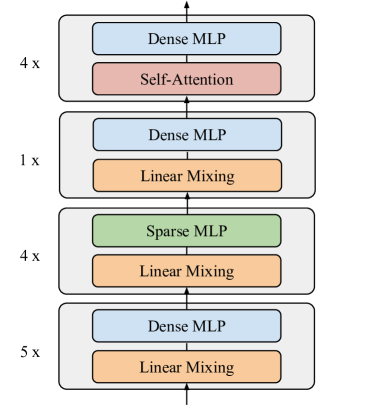
Figure 1: Sparse Mixer encoder blocks for the Base configuration. Layer norms, residual connections, embedding layers and output layers are not shown. The top $K=4$ blocks contain self-attention and dense MLPs; the middle $M=4$ blocks contain mixing and sparse MLPs; and the remaining $L=1$ and $P=5$ blocks contain mixing and dense MLPs.

Our design space for the Sparse Mixer builds off of the stacked encoder blocks of BERT (Devlin et al., 2019), which we use as our canonical Transformer encoder (Vaswani et al., 2017). Each encoder block contains a mixing or self-attention sublayer and a (dense or MoE) MLP sublayer, connected with residual connections and layer norms. We keep the standard BERT input embedding and output projection layers (Devlin et al., 2019); see also Appendix A.1. We arrive at the Sparse Mixer encoder block stack, shown in Figure 1, by carefully ablating through mixing mechanisms, MoE configurations, and model hyperparameters in Section 4.

3.2 MoE

In an MoE layer, we initialize multiple, different instances ("experts") of the layer and perform parallel computations with each instance over separate data shards. The sparsely activated MoE layers therefore have greater capacity than dense layers. As we increase the number of experts, we typically decrease the expert capacity – the number of tokens processed by an individual expert. More specifically, with $E$ denoting the number of experts and $n$ the number of tokens, we set

$$\text{expert capacity}=cf\times n/E,$$

where $cf$ is the scalar capacity factor. For $cf\approx 1$, this allows us to increase model parameter count with minimal increases in FLOPS.

Routing. We use a router or gating function to carefully direct data shards between experts. This follows the intuition that expert A may become specialized at processing inputs in one part of the embedding space, while experts B, C, …are specialized to other parts of the embedding space. It is the router that ensures sparsity by assigning only a subset of tokens to each expert, thereby ensuring that only a subset of parameters are activated for each token.

Router design is an active research area (Lewis et al., 2021; Roller et al., 2021; Zhou et al., 2022; Clark et al., 2022). We limit ourselves to two router types: traditional "Tokens Choose" and "Experts Choose". We follow the standard practice of routing at the token level – the router assigns each token to a subset of experts. Both assignment algorithms first generate router logits by projecting token representations from the embedding dimension, $d_{m}$, to the expert dimension, $E$. We apply a softmax to normalize the logits to a probability distribution. Finally, tokens are assigned to experts using one of the assignment algorithms.

Tokens Choose routing. For Tokens Choose routing Shazeer et al. (2017), each token is assigned to its top-k experts. We focus on top-1 ("Switch") routing (Fedus et al., 2022). Because expert capacities are limited, there is no guarantee that a given token can be routed to its top expert, although any token that fails to reach an expert will still propagate into the next encoder block through the residual connection. There is also no guarantee that a given expert receives at least one token. So, to ensure that compute is efficiently distributed among experts, we include a load balancing loss as in (Shazeer et al., 2017; Fedus et al., 2022).

We can increase expert capacity by increasing the capacity factor, $cf$. This will increase the probability that a given token is routed to its desired experts. Decreasing $cf$ will further sparsify the model and speed up the MoE sublayer. We use Batch Prioritized Routing (Riquelme et al., 2021) to prioritize routing tokens with the highest router probability, rather than simply routing tokens in the left-to-right ordering in the batch.

Experts Choose routing. For the Experts Choose assignment algorithm (Zhou et al., 2022), experts choose their top tokens, rather than tokens choosing experts. This effectively amounts to a transpose of the router probabilities prior to the top-k operation. Each expert performs its top-k operation with k = expert capacity. An individual token may be processed by multiple experts or none at all. Because experts have their choice of tokens and always fill their buffer, increasing the capacity factor, $cf$, will increase both the number of tokens that an expert processes and also the number of experts to which a given token is routed. Because each expert always fills its capacity, no auxiliary loading balancing loss is required.

Token group size. Tokens are subdivided into groups and expert assignment is performed on a per-group basis. A larger group size will result in slower but more accurate top-k and sorting computations, whereas a smaller group size will result in faster but more approximate routing choices. In practice, we find that imperfect routing choices are tolerable and default to a group size of $4096$ tokens.

Parallelization strategies. In this work, we focus on faster, servable architectures using expert and data parallelism. We use data parallelism to shard data across devices, and expert parallelism to partition experts across devices; for example, placing experts 1 and 2 on device 1, experts 3 and 4 on device 2, and so on. Model parallelism is a third axis to shard model weights (matrices) across devices; for example, expert 1 is split across devices 1 and 2, expert 2 is split across devices 3 and 4, and so on. Model parallelism is typically most beneficial for scaling to larger model sizes.

3.3 Mixing

We use simple linear, mixing transformations as drop-in replacements for a subset of the self-attention sublayers. Mixing transformations offer speed for reduced capacity and flexibility. Indeed, the attention mechanism contains four parameterized projections and two dot product operations ("$QK$" and "$V$"), allowing self-attention sublayers to construct representations in a highly expressive, token-dependent basis. On the other hand, the mixing transformations that we investigate are implemented through two, token-independent projections, one along each of the sequence and model dimensions. Fixing the mixing basis, relative to different data inputs, turns out to stabilize the model.

Spectral transformations. We experiment with the Fourier and Hartley transforms (Lee-Thorp et al., 2021). We integrate these transforms through a Fourier sublayer. The Fourier sublayer applies a 1D Discrete Fourier Transform (DFT) along the sequence dimension, $\mathcal{F}_{\textrm{seq}}$, and a 1D DFT along the hidden dimension, $\mathcal{F}_{\textrm{h}}$:

$$y=\Re\left(\mathcal{F}_{\textrm{seq}}\left(\mathcal{F}_{\textrm{h}}(x)\right)\right),$$ (1)

where $\Re$ denotes the real part.

The Hartley sublayer uses Equation (1) with the DFT replaced with the Discrete Hartley Transform, $\mathcal{H}$. We compute the Fourier and Hartley transforms using the Fast Fourier Transform (FFT) (Cooley and Tukey, 1965; Frigo and Johnson, 2005).

In Equation (1), we transform along both the sequence and hidden dimensions. Although the primary purpose of a mixing sublayer is to combine inputs along the sequence dimension, Lee-Thorp et al. (2021) found that also mixing along the hidden dimension improved model quality.

Structured matrix projections. We explore structured matrices under the hypothesis that adding structure to the mixing basis may improve the distribution of output representations. We consider two parameterized, structured matrices: Toeplitz and circulant. A Toeplitz matrix is a matrix in which each diagonal is constant. A circulant matrix is a particular kind of Toeplitz matrix, in which all rows are composed of the same elements but rotated one element to the right relative to the preceding row. For both matrices, the weights are learned. The corresponding mixing sublayer mixes along the sequence and hidden dimension. For example, for the Toeplitz case, we perform:

$$y=\mathcal{T}_{\textrm{seq}}\ \mathcal{T}_{\textrm{h}}\ x,$$ (2)

where $\mathcal{T}_{\textrm{seq}}$ and $\mathcal{T}_{\textrm{h}}$ denote Toeplitz matrices.

Vanilla matrix projections. We also consider "unstructured", fully dense parameterized matrix projections. Following (Lee-Thorp et al., 2021), we call the mixing sublayer arising from this case, the "Linear" sublayer. The Linear sublayer performs the same FLOPS as the structured matrix sublayers (provided the FFT is not used), but is more flexible due to the increased number of matrix weights.

3.4 Implementation

We train and optimize our model on 8 V100 GPUs. We believe that our results are reasonably robust to differing accelerators (e.g. TPU) as almost all of our modifications boil down to accelerator friendly matrix multiplications. In Section 5, we scale our model sizes up and down on TPUs and find that the same favorable efficiency trade-offs persist. We use JAX (Bradbury et al., 2018) in the Flax framework (Heek et al., 2020).

4 Coordinate Descent

We train in a typical transfer learning setting (Devlin et al., 2019): Masked Language Modelling (MLM) and Next Sentence Prediction (NSP) pre-training, followed by fine-tuning on GLUE (Wang et al., 2018) and SuperGLUE (Wang et al., 2019). When comparing models, we always use the exact same setup for all models and baselines. In particular, we follow the pre-training setup in (Devlin et al., 2019) with a few updates: (1) we pre-train on the much larger C4 dataset (Raffel et al., 2020); (2) we use a $32000$ SentencePiece vocabulary model (Kudo and Richardson, 2018) trained on a $100$ million sentence subset of C4; and (3) we use a smaller batch size of $64$ (Devlin et al. (2019) uses $256$). We use a sequence length of $512$ throughout pre-training. Experiments are run on $8$ V100 GPU chips, except for the scaling experiments (Section 5) which are run on 32 TPU v3 chips.

In this section, we follow a "coordinate descent" through our model configurations until we arrive at the final Sparse Mixer design. Given the large number of model hyperparameters to explore, we perform multiple parameter searches in parallel. For example, the model shape and MoE configurations are explored independently and then the most promising configurations from each program are combined.

Table 1: Average accuracy metrics and median pre-training step speeds for mixing models. The "Fourier" model is identical to FNet (Lee-Thorp et al., 2021). Speed-ups relative to BERT (see Table 8) are shown in parentheses. The best metrics are highlighted in boldface, while the second best metrics are underlined. Stars indicate the selected configurations.

	Accuracy (%)			Speed
Model	GLUE	MLM	NSP	(ms/batch)
Fourier	78.4	55.7	75.4	173 (1.75x)
Hartley $\star$	78.0	58.5	74.9	172 (1.77x)
Circulant	75.1	58.3	75.6	200 (1.52x)
Toeplitz	76.5	57.7	76.5	200 (1.52x)
Linear $\star$	77.7	57.6	77.4	200 (1.52x)

For our coordinate descent study, we only pre-train for $500k$ steps, which we found to be reasonably indicative of model performance. Models are fine-tuned with the same batch size ($64$) on the Validation split of each respective GLUE task for $5$ epochs and the best result for each task is selected from across three default base learning rates, adapted from Devlin et al. (2019): $\{10^{-5},5\cdot 10^{-5},10^{-4}\}$. Our final model is pre-trained for longer and is evaluated on both GLUE and SuperGLUE for a broader set of training configurations in Section 5.

We prioritize efficiency – speed and accuracy. We use pre-training step speed as a proxy for model latency. We rely on downstream average GLUE scores as our primary accuracy metric, but fallback to upstream MLM and NSP accuracies when GLUE scores between model variants are similar. Additional coordinate descent experiments are summarized in Appendix A.2, and full GLUE results for all coordinate descent experiments are provided in Appendix A.3.

4.1 Mixing

Mixing mechanisms. We compare the mixing mechanisms discussed in Section 2. For each mixing model, we first replace all self-attention sublayers with the corresponding mixing sublayer. The results are shown in Table 1. The spectral models (Fourier and Hartley) perform the best on GLUE. The Linear model slightly under-performs the spectral models, while the structured mixing models (Circulant and Toeplitz) perform worst on GLUE. The spectral methods, efficiently implemented using FFTs, are the fastest.

Hybrid mixing-attention. We choose two strong representative candidates from Table 1, namely the Hartley and Linear models, and replace a subset of the topmost mixing sublayers with self-attention. The results are summarized in Table 2.

Table 2: Metrics for hybrid attention-mixing models. Hartley-$k$ denotes a model with $k$ self-attention sublayers and $12-k$ Hartley sublayers.

	Accuracy (%)			Speed
Model	GLUE	MLM	NSP	(ms/batch)
Hartley-0	78.0	58.5	74.9	172 (1.76x)
Hartley-1	78.0	51.9	75.3	183 (1.66x)
Hartley-2	81.1	61.3	79.8	193 (1.57x)
Hartley-3	77.9	50.3	76	204 (1.49x)
Hartley-4	82.7	62.6	81	216 (1.41x)
Hartley-6	82.9	63.5	81.2	234 (1.30x)
Linear-0	77.7	57.6	77.4	200 (1.51x)
Linear-1	78.1	62.5	78.3	208 (1.46x)
Linear-2	82.8	62.8	81	218 (1.40x)
Linear-3	82.8	63.3	81.6	226 (1.35x)
Linear-4 $\star$	83.4	63.6	81.7	235 (1.29x)
Linear 6	83.6	64	81.7	251 (1.21x)

Once we include self-attention, we see that the hybrid Linear model offers larger quality gains than the hybrid Hartley model. Even though the hybrid Hartley models are faster, an iso-speed comparison still suggests that the hybrid Linear models are more efficient. For example, Hartley-6 and Linear-4 having roughly the same speed, but the Linear-4 model is more accurate. Hence, we opt to use the Linear-4 model. In Appendix A.2 (Table 11), we show that we get best accuracy when the self-attention sublayers at placed in the topmost layers.

4.2 Model shape

All model shape experiments are run in parallel and start from the Linear-4 configuration.

Table 3: Varying the model dimension, $d_{m}$. As in the Transformer, we set the model and embedding dimension to be equal. For the self-attention sublayers, we fix the number of self-attention heads to $d_{m}/64$.

	Accuracy (%)			Speed
$d_{m}$	GLUE	MLM	NSP	(ms/batch)
768	83.4	63.6	81.7	235 (1.29x)
512 $\star$	83.0	62.5	80.9	161 (1.89x)
256	80.7	58.9	78.4	91 (3.34x)
128	71.6	54	73.8	58 (5.29x)

Model dimensions. In seeking a more efficient model, we attempt to slim our model down both by decreasing the model dimension (Table 3) and the intermediate MLP activation dimension (Table 12 in Appendix A.2). For each coordinate, we find that there are cutoffs ($d_{ff}=2048$ and $d_{m}=512$) below which model quality drops drastically. We select these cutoffs as our optimal model shape values. It is in decreasing these two hyperparameters that we obtain the biggest speed-up in our model. However, there is a material degradation in quality that must be compensated by the increased capacity from the MoE sublayers in Section 4.3.

Number of layers. We vary the number of layers in Table 13 in Appendix A.2. We opt for $14$ layers, beyond which we do not see quality gains.

Table 4: Accuracy and speed metrics for Top-1 Tokens Choose (TC) and Experts Choose (EC) routing.

	Accuracy (%)			Speed
Router	GLUE	MLM	NSP	(ms/batch)
TC	83.4	64	80.8	280 (1.09x)
EC $\star$	83.5	64.6	81.2	283 (1.08x)

4.3 MoE

Our starting configuration for our MoE ablations is the Linear-4 configuration with every other dense MLP sublayer replaced by an MoE sublayer ($6$ MoE sublayers) and $16$ experts in each MoE sublayer. We performed the MoE experiments in parallel to the model shape optimizations, so all MoE ablations are performed on a default Base sized model with $12$ layers, $d_{ff}=3072$ and $d_{m}=768$.

As in (Zoph et al., 2022), we find that we must adjust the fine-tuning learning protocol to better transfer any MoE MLM pre-training gains downstream. In particular, our MoE encoder models benefit from larger base learning rates ($\{10^{-4},5\cdot 10^{-4},10^{-3}\}$) and larger dropout rates ($0.2$) for experts; see Appendix A.4 for a comparison of learning rates and expert dropout rates. For our final model comparison with BERT in Section 5, we consider a wide range of base learning rates for all models.

Routers. Routing mechanisms are compared in Table 4. We select Experts Choose routing as it obtains slightly higher accuracy results and does not require configuring a load balancing loss.

Table 5: Varying the number and layout of MoE sublayers. Layout definition: 6-BOTTOM (first $6$ layers), 6-MIDDLE (middle $6$ layers) or 6-MIXED (every odd layer), 6-MIXED-odd (every even layer), and 6-TOP (final $6$ layers). The number of experts and the expert capacity – the number of tokens processed by each expert – is fixed. Each MoE layer adds some compute and device communication overhead, slowing the model.

	Accuracy (%)			Speed
Config	GLUE	MLM	NSP	(ms/batch)
2-MIXED	83.6	63.6	81.3	246 (1.23x)
4-MIXED $\star$	83.6	63.9	81.3	264 (1.15x)
6-MIXED	83.5	64.6	81.2	283 (1.08x)
12-MIXED	83.1	64.9	81.4	352 (0.86x)
6-BOTTOM	83.2	62.7	81.4	289 (1.05x)
6-MIDDLE $\star$	83.9	64	81.7	284 (1.08x)
6-MIXED	83.5	64.6	81.2	283 (1.08x)
6-MIXED-odd	83.2	64.8	81.6	292 (1.04x)
6-TOP	83.4	65.4	81.2	287 (1.06x)

Table 6: GLUE results on the Validation split. We report F1/accuracy scores for QQP and MRPC, Spearman correlations for STS-B and accuracy scores for all other tasks. The MNLI accuracy metrics are reported by the match/mismatch splits.

Model	MNLI	QQP	QNLI	SST-2	CoLA	STS-B	MRPC	RTE	Avg.
BERT	81.3 / 81.8	86.7 / 90.3	88.9	91.1	77.6	87.3	90.5 / 86.8	69.7	84.7
Sparse Mixer	80.7 / 81	87.1 / 90.5	89.1	90.9	79	88.1	90.4 / 86.3	72.2	85.0

Table 7: SuperGLUE Validation results. We report macro-F1 scores for CB, micro-F1/exact match scores for MultiRC, F1/exact match scores for ReCoRD, and accuracy scores for all other tasks.

Model	BoolQ	CB	COPA	MultiRC	ReCoRD	RTE	WiC	Avg.
BERT	74.6	86.4 / 85.7	58	74.1 / 26.2	68.6 / 52.2	65	65.7	65.7
Sparse Mixer	74.4	93.3 / 92.9	62	72.4 / 22.5	65.9 / 49.2	64.6	66.5	66.4

MoE layers. In Table 5, we vary the number of MoE sublayers and the layout of those layers within the model. As we increase the number of MoE layers, MLM accuracy improves, but these pre-training gains do not always lead to better GLUE performance. This was a general trend that we observed; see also Appendix A.2 and (Zoph et al., 2022). We opt for 4 MoE layers, which performs well on GLUE and better than the 2 MoE sublayer model on the MLM task.

The results of MoE layout experiments are clearer – we opt to use the MIDDLE layout, placing all MoE sublayers in the middle layers of the model. Nevertheless, it is interesting to note that the TOP layout gives a big boost to MLM accuracy, but does not improve downstream GLUE accuracy.

Number of experts. We can increase the number of experts to increase the capacity of the model. For a large number of experts, the computational cost of the routing assignment is more significant, while the training signal to an individual expert becomes too weak to facilitate effective training as each expert processes too small a slice of data. Seeking a compromise between quality and speed, we ultimately opt to use 16 experts. Results are summarized in Table 14 in Appendix A.2.

Expert size. We can control the number of parameters in each expert by varying its $d_{ff}$. In Table 15 (Appendix A.2), we find that: (1) using smaller experts yields a small accuracy drop, but limited speed benefits; and (2) increasing expert size increases MLM accuracy, but not GLUE. So, for simplicity, we opt to keep the expert $d_{ff}$ the same size as the dense $d_{ff}$.

4.4 Sparse Mixer

Putting the preceding results together, we arrive at the Sparse Mixer model in Figure 1:
Shape:  14 layers, 512 $d_{m}$, 2056 $d_{ff}$;
Sparse: 4 MIDDLE MoE, 16 experts, 2056 $d_{ff}$,      EC routing, 1.0 $cf$;
Mixer:   Linear, 4 TOP Attention layers.

Table 8: Model computational characteristics for BERT, Sparse Mixer (SM) and Fast Sparse Mixer (FSM), which is introduced in Section 5. "Size" is the number of model parameters. Run speeds are measured by inference speed per example and pre-training step speed per example.

	GFLOPS	Size	Inference	Training
Model	(/ex)	(M)	(ms/ex)	(ms/ex)
BERT	102	112	1.34	4.75
SM	73	180	0.84 (1.61x)	2.87 (1.65x)
FSM	60	180	0.68 (1.98x)	2.51 (1.89x)

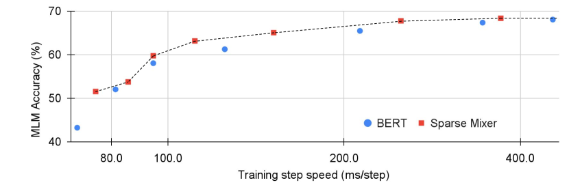
Figure 2: Pre-training Speed-accuracy trade-offs for Sparse Mixer and BERT. The corresponding model configurations are shown in Table 20 in Appendix A.5. The dashed line shows the Pareto efficiency frontier, indicating the best trade-offs. All models are trained on 32 TPU v3 chips. To better utilize the increased number of devices, we use a larger batch size of 256 but train for fewer (250k) steps.

5 Evaluating Sparse Mixer

Full training comparison with BERT. When comparing Sparse Mixer and BERT, both models are pre-trained on C4 for the full $1M$ steps, with batch size $64$, and then evaluated on both GLUE and SuperGLUE for a larger range of fine-tuning batch sizes (16, 32, and 64) and base learning rates ($\{10^{-5},5\cdot 10^{-5},10^{-4},5\cdot 10^{-4},10^{-3}\}$). The best results across all learning rates (for each task) and batch sizes (for all tasks) are shown in Tables 6 and 7; see Appendix A.3 for results for all batch sizes.

BERT and Sparse Mixer’s GLUE scores are very similar, although they diverge a little more on SuperGLUE, where Sparse Mixer performs particularly well on the CB task, but underperforms BERT on the multi-label MultiRC and ReCoRD tasks.

Scaling the Sparse Mixer. Tables 6-8 indicate that the Sparse Mixer is more efficient than BERT in the Base configuration. In Figure 2, we compare BERT and Sparse Mixer across a selection of model sizes. We use MLM accuracy as a proxy for model accuracy and pre-training step speed as a proxy for overall model speed. Pre-training step speed is a good proxy for inference speed (see Table 8). MLM accuracy is only indicative of downstream accuracy. We construct an analogous speed-accuracy figure for NSP accuracy in Figure 4 in Appendix A.5. These caveats aside, Figure 2 suggests that Sparse Mixer’s favorable speed and accuracy extends to other model sizes, as it defines the efficiency frontier across all model sizes considered.

Table 9: Fast Sparse Mixer (FSM). The default Sparse Mixer (SM) uses a capacity factor ($cf$) of 1 and a routing group size ($g$) of 4096. Several less favorable configurations are omitted.

	Accuracy (%)		Speed
Model	GLUE	SuperGLUE	(ms/batch)
BERT	84.7	65.7	304
SM	85.0	66.4	184 (1.65x)
FSM ($cf$=$0.5$)	84.7	65.6	161 (1.89x)
$g$=$2048$	84.5	65.1	173 (1.75x)
$cf$=$0.75$,$g$=$2048$	84.3	65.2	165 (1.84x)

Table 10: Stability of BERT, sparse BERTs and Sparse Mixer (SM). BERT-$k$ denotes a BERT model with $k$ MoE layers. The "unstable" runs experience gradient blow-up and fail to converge to an optimal loss (or converge at all). We use batch sizes of 64 and 256. Accuracy and speed metrics are reported for 64 batch runs.

	Stable		Accuracy (%)		Speed
Model	64	256	GLUE	S.GLUE	(ms/batch)
BERT	3/4	4/4	84.7	65.7	304
SM	4/4	4/4	85.0	66.4	184 (1.65x)
BERT-4	0/4	0/4	-	-	-
BERT-12	1/4	0/4	84.1	60.9	426 (0.71x)

Trading accuracy for more speed. We design an even sparser model by decreasing the expert capacity factor. This decreases the number of tokens that each expert processes and yields significant speed-ups for a limited quality degradation: for a minor (0.2%) accuracy drop on SuperGLUE relative to BERT, a Sparse Mixer with capacity factor of 0.5 trains 89% faster and runs inference 98% faster; see Table 8. We name this variant of the model Fast Sparse Mixer. We also experiment with decreasing the token routing group size, but this leads to larger quality drops.

Stability. Table 10 compares the stability of Sparse Mixer, BERT and "sparse BERTs" – MoE variants of BERT. Sparse Mixer is very stable, even relative to (dense) BERT. The sparse BERTs are highly unstable, with only one stable run that ultimately yields a slow model that significantly underperforms BERT. We hypothesize that the Sparse Mixer’s improved stability is due to replacing most of the self-attention sublayers with mixing, which constrains the model to a less variable mixing basis.

6 Conclusions

Mixing transformations and MoE play well together. Utilizing MoE for capacity and mixing for speed and stability, we introduced the Sparse Mixer – a model that slightly outperforms BERT on GLUE and SuperGLUE, but more importantly trains 65% faster and runs inference 61% faster. We also presented a faster variant, Fast Sparse Mixer, that marginally under-performs BERT on SuperGLUE, but trains and runs nearly twice as fast: 89% faster training and 98% faster inference. Sparse Mixer overcomes many of the speed and stability concerns of MoE models and offers the prospect of serving sparse student models.

Limitations

Encoder only model. We have focused our work on BERT-like models as they are extremely wide used. However, this limits our focus to encoders, which are not suitable for generative tasks. Sparse mixer encoder-decoder and decoder-only models are, in principle, straightforward extensions: Linear decoders can be designed by “causally” masking the Linear matrix and encoder-decoder mixing can also be designed with careful masking. However, we suspect that parts of the coordinate descent program will need to be repeated. For example, evidence suggests that cross-attention may be crucial to performance of encoder-decoder models (You et al., 2020). Nevertheless, we hope that the current Sparse Mixer recipe acts as a starting point and a roadmap for generalizing to other architectures.

More diverse tasks and learning frameworks. We only evaluated Sparse Mixer on GLUE and SuperGLUE. It would be good to look at broader set of tasks, including Q&A. We also stuck to the original BERT training setup (Devlin et al., 2019), but there are potential training regime improvements that could be introduced, such as training for much longer as for RoBERTa (Liu et al., 2019b) or using the ELECTRA generator-discriminator training setup (Clark et al., 2020).

"Manual ML". In designing the Sparse Mixer architecture, we have optimized the model configuration one hyperparameter coordinate at a time. So while our manual gradient descent offers interpretability and pedagogical insight, it is potentially sub-optimal. It would be exciting to see future work expand both the coordinate space and jointly optimize multiple coordinates using Automated Machine Learning (AutoML) (Thornton et al., 2013; Liu et al., 2019a; Peng et al., 2020).

Long input sequences. Because of the presence of attention layers, Sparse Mixer will not scale as well as efficient Transformers to long sequence inputs. This could be compensated by dropping in efficient approximations of the attention mechanism Tay et al. (2021a).

Appendix A Appendices

A.1 Base architecture

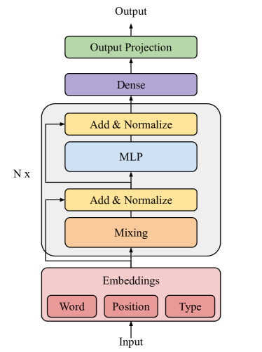
Figure 3: Block based encoder architecture. The model has $N$ encoder blocks, each containing mixing and MLP sublayers. Each MLP sublayer may be sparse or dense. Each mixing sublayer may use self-attention or a mixing transformation.

Our design space for the Sparse Mixer builds off of the stacked encoder blocks of BERT (Devlin et al., 2019) in Figure 3. Each encoder block contains a mixing sublayer and an MLP sublayer, connected with residual connections and layer norms. We keep the standard BERT input embedding and output projection layers (Devlin et al., 2019).

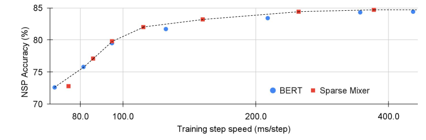
Figure 4: NSP pre-training Speed-accuracy trade-offs for Sparse Mixer and BERT. The dashed line shows the Pareto efficiency frontier, indicating the best trade-offs.

A.2 Exploring more coordinates

Table 11: Average accuracy metrics and median pre-training step speeds for varying where the self-attention sublayer are placed within the Linear-4 model. Speed-ups relative to BERT (see Table 8) are shown in parentheses. The best metrics are highlighted in boldface. The star indicate the selected configuration.

	Accuracy (%)			Speed
Layout	GLUE	MLM	NSP	(ms/batch)
BOTTOM	82	62.6	81	236 (1.29x)
MIDDLE	82.4	63.2	80.7	236 (1.29x)
MIXED	82.7	63.6	81.1	235 (1.29x)
TOP $\star$	83.4	63.6	81.7	235 (1.29x)

Attention sublayer layout. Where should the $4$ attention sublayers be placed within the model? We check whether it best to place the $4$ self-attention sublayers at the TOP (final $4$ layers), BOTTOM (first $4$ layers), MIDDLE (middle $4$ layers) or MIXED (every third layer). Table 11 shows that the TOP layout is best.

Mixing dead ends. We tested two other mixing modifications that yielded no quality (or latency) gains: (1) adding a bias term to the mixing transformations, and (2) adding dropout during fine-tuning to the mixing sublayers.

Intermediate activation dimension. Below $d_{ff}=2048$, the model quality drops significantly. We select this cutoff as our optimal model MLP dimension.

Number of layers. We do not see quality gains beyond $14$ layers. Because we plan to thin out our model (decrease $d_{ff}$ and $d_{m}$), we opt for slightly increasing the number of layers to 14.

Table 12: Metrics for various intermediate MLP activation dimensions, $d_{ff}$.

	Accuracy (%)			Speed
$d_{ff}$	GLUE	MLM	NSP	(ms/batch)
3072	83.4	63.6	81.7	235 (1.29x)
2560	83.2	62.2	81.1	208 (1.46x)
2048 $\star$	83.5	62	81	189 (1.61x)
1024	82.9	60.7	80.6	146 (2.09x)
768	82.8	60.4	80.7	135 (2.24x)

Table 13: Varying the number of model layers. The results are for post-layer normalization, as in BERT. We obtained similar results for pre-layer normalization.

	Accuracy (%)			Speed
Layers	GLUE	MLM	NSP	(ms/batch)
6	82.3	62.4	80.9	142 (2.14x)
10	83.6	63.4	81.4	201 (1.51x)
12	83.4	63.6	81.7	235 (1.29x)
14 $\star$	83.8	64	81.6	260 (1.17x)
18	83.8	63.9	81.5	320 (0.95x)

Number of experts. In Table 14, we increase the number of experts to increase the capacity of the model. As discussed in Section 3.2, we simultaneously decrease each expert’s capacity (the number of tokens it processes) to prevent FLOPS from growing. We suspect that, for a large number of experts, the training signal to an individual expert becomes too weak to facilitate effective training as each expert processes too small a slice of data. This is particularly apparent on downstream tasks where there are fewer training examples. Furthermore, for a large number of experts ($\geq 64$), the computational cost of the routing assignment starts to become significant. Seeking a compromise between quality and speed, we ultimately opt to use 16 experts.

Table 14: Increasing the number of experts. These experiments were run in parallel to those of Table 5 and therefore use the default 6-MIXED setup. Speed-ups relative to BERT (see Table 8) are shown in parentheses. Based on the speed slowdown for 64 experts and the relatively weak performance of 32 experts, we did not evaluate 64 experts on GLUE.

	Accuracy (%)			Speed
Experts	GLUE	MLM	NSP	(ms/batch)
8	83.3	64.1	81.2	277 (1.10x)
16 $\star$	83.5	64.6	81.2	283 (1.08x)
32	83.3	65.1	81.3	292 (1.04x)
64	-	65.4	80.9	327 (0.93x)

Expert size. The number of parameters in each expert can be controlled by varying its intermediate activation dimension, $d_{ff}$. If we can maintain accuracy while decreasing the size of each expert, that will speed up our model. On the other hand, if we can achieve large accuracy gains by increasing the size of experts, we can potentially use that to offset shrinking the rest of the model; for example, by constructing a "thin", fast model with only a few "heavy", high capacity MoE layers. In Table 15, we see that neither of these scenarios plays out cleanly: (1) Using smaller experts ($d_{ff}=1536$) yields only a small accuracy drop, but little speed benefit. (2) As was the case for increasing the number of MoE sublayers and the number of experts, increasing expert size increases MLM accuracy, but the results do not translate downstream to GLUE. For simplicity, we opt to keep the expert $d_{ff}$ the same size as the dense $d_{ff}$, which is optimized in Section 4.2.

Table 15: Varying the size of experts by varying each expert’s intermediate activation dimension, $d_{ff}$. These experiments were run in parallel to those of Table 5 and therefore use the default 6-MIXED setup.

	Accuracy (%)			Speed
$d_{ff}$	GLUE	MLM	NSP	(ms/batch)
1536	83.4	64	81.1	274 (1.11x)
3072 $\star$	83.5	64.6	81.2	283 (1.08x)
6144	83.3	65.3	81.5	305 (1.00x)
12288	83.1	65.9	81.7	350 (0.87x)

MoE dead ends. (1) Changing the expert nonlinearity from GELU to RELU had little effect on downstream performance. Changing the nonlinearity to GEGLU (GELU Gated Linear Units) (Shazeer, 2020) only slowed down the model. (2) Although the router z-loss had little effect on model performance, we included it for potential stability benefits. (3) Fedus et al. (2022) recommend using a smaller scaled weight initialization to provide stability to MoE encoder-decoder models, especially in larger configurations. However, we obtained the best results, for our encoder-only model, with BERT’s default kernel initialization.

Table 16: Full GLUE results (Validation split) for all coordinate descent experiments. See the corresponding table for descriptions of each configuration. For dense models (Tables 1, 2, 11, 12, 3 and 13), we report the best scores across $\{10^{-5},5\cdot 10^{-5},10^{-4}\}$ base learning rates, while for MoE models (Tables 4, 5, 14 and 15), we use $\{10^{-4},5\cdot 10^{-4},10^{-3}\}$. We report F1/accuracy scores for QQP and MRPC, Spearman correlations for STS-B and accuracy scores for all other tasks. The MNLI accuracy metrics are reported by the match/mismatch splits. The top two average scores for each experiment set are boldfaced/underlined.

Table	Model	MNLI	QQP	QNLI	SST-2	CoLA	STS-B	MRPC	RTE	Avg.
	Fourier	74.5 / 75.6	84.3 / 88.3	82.2	88.5	69.6	80.2	83.5 / 73.8	62.1	78.4
	Hartley	75 / 75.7	84.4 / 88.1	82.6	87.7	69.4	80.9	82.2 / 72.1	59.9	78.0
1	Circulant	69.7 / 70.9	83.3 / 87.6	76	89.2	76.1	56.1	82.7 / 71.8	62.8	75.1
	Toeplitz	73.2 / 73.5	84.2 / 88.3	78.1	88.6	73	66.1	82.6 / 71.6	62.8	76.5
	Linear	73.4 / 74.3	84.3 / 88.2	80.2	89.6	74.6	68.2	83.5 / 75.2	63.5	77.7
	Hartley-0	75 / 75.7	84.4 / 88.1	82.6	87.7	69.4	80.9	82.2 / 72.1	59.9	78.0
	Hartley-1	72.7 / 73.6	83.9 / 87.8	82.1	86.8	71.1	79.5	82.8 / 75.7	62.1	78.0
	Hartley-2	79.5 / 78.3	86 / 89.7	86.2	89.3	74	85.7	84.6 / 76.7	62.1	81.1
	Hartley-3	74.2 / 75	83.5 / 87.9	81.9	88.8	70.4	78.3	83.1 / 73.3	61	77.9
	Hartley-4	79 / 80.2	86.7 / 90.1	87.2	89.9	75.2	86.1	87.5 / 82.4	65	82.7
2	Hartley-6	80 / 81	86.7 / 90.2	88	90.7	75.3	86.5	87.3 / 81.9	64.6	82.9
	Linear-0	73.4 / 74.3	84.3 / 88.2	80.2	89.6	74.6	68.2	83.5 / 75.2	63.5	77.7
	Linear-1	74.4 / 74.9	84.9 / 88.8	81.8	91.4	78	69	83.4 / 73	59.9	78.1
	Linear-2	80.1 / 80.5	87 / 90.3	87.6	90	78.2	86.7	85.3 / 78.2	66.8	82.8
	Linear-3	80.2 / 81	87 / 90.4	87.3	90.5	77.9	87.8	84.7 / 78.4	66.1	82.8
	Linear-4	80.4 / 81.2	87.2 / 90.4	88	91.3	76.7	87.4	87.2 / 81.6	65.7	83.4
	Linear-6	80.7 / 81.6	87.3 / 90.6	87.8	90.5	78.2	87.2	88.7 / 83.6	63.9	83.6
	BOTTOM	79.1 / 79.6	86.8 / 90.3	86.2	90.7	73.2	85.5	87.5 / 82.1	61	82.0
11	MIDDLE	80 / 80.3	86.7 / 90.3	86.5	89.2	72.2	86.3	88.3 / 83.1	63.5	82.4
	MIXED	79.5 / 80.3	87.1 / 90.5	87.6	90.7	75	85	87.1 / 82.1	64.6	82.7
	TOP	80.4 / 81.2	87.2 / 90.4	88	91.3	76.7	87.4	87.2 / 81.6	65.7	83.4
	$d_{ff}$=3072	80.4 / 81.2	87.2 / 90.4	88	91.3	76.7	87.4	87.2 / 81.6	65.7	83.4
	$d_{ff}$=2560	80.3 / 81.5	87.2 / 90.5	88.3	91.6	77.8	86.9	85.5 / 79.2	66.1	83.2
12	$d_{ff}$=2048	80.4 / 81.1	87.1 / 90.5	87.7	91.3	76.6	87	87.8 / 82.4	66.8	83.5
	$d_{ff}$=1024	79.9 / 80.8	87 / 90.3	87.3	90	76.3	87.4	87.7 / 81.9	62.8	82.9
	$d_{ff}$=768	80.1 / 81.1	86.7 / 90.2	87.4	89.7	75.7	86.6	87.7 / 82.6	62.8	82.8
	$d_{m}$=768	80.4 / 81.2	87.2 / 90.4	88	91.3	76.7	87.4	87.2 / 81.6	65.7	83.4
3	$d_{m}$=512	80.1 / 80.9	86.6 / 90.1	87.4	90.8	77	87.2	86.3 / 80.1	66.4	83.0
	$d_{m}$=256	77.9 / 78.5	84.4 / 88.1	85.2	89.8	73.9	83.8	84.5 / 76	66.1	80.7
	$d_{m}$=128	74.9 / 75.9	84.2 / 88.1	84	88	69.8	9.7	82.1 / 70.3	60.3	71.6
	6 layers	79.9 / 81	87 / 90.4	87.3	90	76	86.7	85.1 / 76.5	65	82.3
	10 layers	80.7 / 81.6	87.1 / 90.4	87.5	87.5	76.5	87.2	90.2 / 86.3	64.3	83.6
13	12 layers	80.4 / 81.2	87.2 / 90.4	88	91.3	76.7	87.4	87.2 / 81.6	65.7	83.4
	14 layers	80.5 / 81.7	87.2 / 90.6	88.1	90.4	78.4	87.8	87.2 / 81.4	68.2	83.8
	18 layers	81.1 / 81.9	87.1 / 90.5	87.7	90.6	79.2	87.3	87 / 82.6	67.2	83.8
4	Tokens Choose	80.2 / 81.2	86.7 / 90.2	87.8	90.1	77.4	87.3	87.6 / 82.4	66.4	83.4
	Experts Choose	80.4 / 81.1	86.8 / 90.2	87.5	90.6	75.9	84.9	88.7 / 83.6	68.6	83.5
	2-MIXED	80.6 / 81.3	87.1 / 90.5	87.1	90.9	76.7	86.6	88 / 82.4	68.2	83.6
	4-MIXED	80.7 / 80.8	86.7 / 90.2	87.3	90.8	76.8	87.5	88 / 82.4	68.2	83.6
	6-MIXED	80.4 / 81.1	86.8 / 90.2	87.5	90.6	75.9	84.9	88.7 / 83.6	68.6	83.5
	12-MIXED	80 / 80.2	86.7 / 90.1	86.3	90.7	75.5	87.5	87.7 / 82.1	66.8	83.1
5	6-BOTTOM	79.9 / 81	86.9 / 90.3	86.9	90.3	76.1	87.1	87.9 / 82.6	66.4	83.2
	6-MIDDLE	80.3 / 80.9	90.6 / 87.2	87.6	90.7	77.6	86.9	89.7 / 85.3	66.4	83.9
	6-MIXED	80.4 / 81.1	86.8 / 90.2	87.5	90.6	75.9	84.9	88.7 / 83.6	68.6	83.5
	6-MIXED$\ast$	80.2 / 81.4	87 / 90.4	87.6	90.8	75.5	86.6	88.2 / 82.8	65.0	83.2
	6-TOP	80.5 / 81.1	86.5 / 90	87.6	90.5	77.3	85.8	87.7 / 82.8	67.1	83.4
	8 experts	80.4 / 81.4	86.2 / 89.8	88	90.9	75.7	86.7	88.3 / 83.1	65.7	83.3
14	16 experts	80.4 / 81.1	86.8 / 90.2	87.5	90.6	75.9	84.9	88.7 / 83.6	68.6	83.5
	32 experts	80.4 / 81.4	86.8 / 90.2	87.4	91.1	78.3	86.7	87 / 81.4	65.3	83.3
	$d_{ff}$=1536	80.6 / 81.3	86.8 / 90.2	87.2	90.6	76.5	85.5	87.7 / 82.4	68.6	83.4
15	$d_{ff}$=3072	80.4 / 81.1	86.8 / 90.2	87.5	90.6	75.9	84.9	88.7 / 83.6	68.6	83.5
	$d_{ff}$=6144	80.3 / 81.4	87.1 / 90.4	87.8	90.6	76.4	87.3	87.3 / 80.9	67.1	83.3
	$d_{ff}$=12288	80.7 / 81.9	85.9 / 89.7	87.7	90.9	77.9	87.2	85.6 / 79.7	67.1	83.1

Table 17: GLUE results (Validation split) for final comparison of BERT, Sparse Mixer (SM), Fast Sparse Mixer (FSM) and other variants for different batch sizes. See the corresponding table for descriptions of each configuration. For each task, we select the best result across the base learning rates $\{10^{-5},5\cdot 10^{-5},10^{-4},5\cdot 10^{-4},10^{-3}\}$. The highest average score for each model (across the three batch sizes) is highlighted in boldface.

Table	Model	Batch	MNLI	QQP	QNLI	SST-2	CoLA	STS-B	MRPC	RTE	Avg.
		16	81.3 / 81.8	86.7 / 90.3	88.9	91.1	77.6	87.3	90.5 / 86.8	69.7	84.7
	BERT	32	81.2 / 81.5	86.9 / 90.3	88.6	91.3	77.6	87.4	90.4 / 86.5	70	84.7
7		64	81.3 / 81.4	87.4 / 90.7	88.7	90.7	77.9	87.5	89.1 / 84.8	70	84.5
		16	80.8 / 81.4	86.9 / 90.2	89.3	91.5	79.2	87.7	90 / 85.8	69.7	84.8
	SM	32	80.7 / 81.4	86.9 / 90.3	88.7	90.6	79.3	87.7	90.4 / 86	70.4	84.8
		64	80.7 / 81	87.1 / 90.5	89.1	90.9	79	88.1	90.4 / 86.3	72.2	85.0
		16	81.2 / 81.5	90.3 / 86.8	89.0	90.9	78.7	87.5	90.2 / 86.3	69.7	84.7
	SM $cf$=$0.5$	32	80.8 / 81.1	90.4 / 86.9	89.0	90.4	78.6	87.9	90.8 / 86.8	68.6	84.7
	(FSM)	64	80.6 / 81.2	90.5 / 87.3	88.5	90.9	78.8	88.7	89.6 / 85	69	84.6
		16	80.8 / 81.7	86.6 / 90.2	88.8	90.8	78.3	88	89.1 / 84.3	70.4	84.5
	SM $g$=$2048$	32	80.5 / 81.6	86.6 / 90.3	88.5	90.5	77.7	87.9	89.4 / 85	69.3	84.3
9		64	81.2 / 81.7	87.1 / 90.4	88.6	90.5	78.2	88.7	88.8 / 84.1	68.6	84.4
		16	80.1 / 80.7	86.8 / 90.2	88.3	91.7	76.4	86.9	88.4 / 83.3	68.6	83.8
	SM $g$=$1024$	32	80.7 / 81	86.9 / 90.3	88.2	90.6	77.3	87.3	88.7 / 83.6	68.6	83.9
		64	80.3 / 80.9	90.4 / 86.9	88.2	90.5	78.2	87.7	88.5 / 83.6	70.4	84.1
		16	80.1 / 81.1	86.8 / 90.4	88.4	90.9	76.4	87.7	88.6 / 83.8	67.9	83.8
	SM $cf$=0.75,	32	80.6 / 80.9	87 / 90.4	88.2	90.8	76.6	88.5	88.3 / 83.6	68.6	84.0
	$g$=$2048$	64	80.1 / 81.3	87.3 / 90.6	88.4	91.3	78	88.2	89 / 84.3	69	84.3
		16	80.7 / 81.2	90.5 / 87	88.2	90.8	78.1	87	88.7 / 83.8	69	84.1
10	BERT-12	32	80.9 / 81.3	87.1 / 90.5	88.2	91.2	78.4	87.1	88 / 82.8	65.3	83.7
		64	80.9 / 80.7	86.5 / 90.1	88.5	90.9	79.1	87.2	87.4 / 81.8	65.7	83.5

Table 18: SuperGLUE results (Validation split) for final comparison of BERT, Sparse Mixer (SM), Fast Sparse Mixer (FSM) and other variants for different batch sizes. See the corresponding table for descriptions of each configuration. We report macro-F1 scores for CB, micro-F1/exact match scores for MultiRC, F1/exact match scores for ReCoRD, and accuracy scores for all other tasks. For each task, we select the best result across the base learning rates $\{10^{-5},5\cdot 10^{-5},10^{-4},5\cdot 10^{-4},10^{-3}\}$. The highest average score for each model (across the three batch sizes) is highlighted in boldface.

Table	Model	Batch	BoolQ	CB	COPA	MultiRC	ReCoRD	RTE	WiC	Avg.
		16	74.6	86.4 / 85.7	58	74.1 / 26.2	68.6 / 52.2	65	65.7	65.7
	BERT	32	72.9	85 / 85.7	61	73.7 / 25.6	70.4 / 54.4	58.5	67.9	65.5
7		64	71.3	75.2 / 80.4	66	71.7 / 21.3	69 / 52.7	62.5	67.9	63.8
		16	74.4	93.3 / 92.9	62	72.4 / 22.5	65.9 / 49.2	64.6	66.5	66.4
	SM	32	73.4	86.5 / 87.5	62	72.8 / 23.4	66.3 / 49.6	67.9	66	65.5
		64	72.4	89.7 / 89.3	59	72.6 / 23.3	65.7 / 48.9	68.6	61.8	65.1
		16	73.5	85.2 / 85.7	69	71.6 / 21.1	65.6 / 48.8	67.9	67.7	65.6
	FSM	32	74.3	82.3 / 85.7	56	71.8 / 21.5	63.8 / 46.9	67.1	62.4	63.2
	(SM w/ $cf$=$0.5$)	64	73.2	87.8 / 87.5	58	70.1 / 19.9	65.3 / 48.5	68.2	62.7	64.1
		16	74.4	85.7 / 86.1	64	70.6 / 20	63.2 / 46.2	66.8	61.4	63.8
	SM w/ $g$=$2048$	32	74.1	82.8 / 83.9	63	70.7 / 20.9	63.6 / 46.7	66.8	62.2	63.5
9		64	74.2	85.2 / 89.3	64	71.1 / 20.8	66.6 / 49.9	69	60.7	65.1
		16	73.9	78.7 / 80.4	63	70 / 18.7	62.8 / 45.8	64.3	63.5	62.1
	SM w/ $g$=$1024$	32	73.4	86.6 / 85.7	64	70.1 / 18.4	64.5 / 47.6	66.4	61.4	63.8
		64	73.6	86.9 / 85.7	61	69.2 / 19.4	64.8 / 47.9	68.6	63	64.0
		16	73.1	92 / 89.3	67	69.5 / 19.9	62.4 / 45.4	67.1	66.1	65.2
	SM w/ $cf$=0.75,	32	73	87.7 / 89.3	60	69.6 / 19.9	63.9 / 46.9	66.4	64	64.1
	$g$=$2048$	64	72.4	80.1 / 82.1	62	69 / 18.9	65 / 48.1	67.1	63.3	62.8
		16	73.9	90.5 / 92.9	61	65.3 / 9.5	48.5 / 32	66.8	59.6	60.0
10	BERT-12	32	72.5	92.3 / 92.9	58	69.6 / 15.5	50 / 33.3	65	60.2	60.9
		64	70.1	87.8 / 91.1	66	64.9 / 6.8	45.4 / 29.5	65.7	61	58.8

A.3 Full GLUE and SuperGLUE results

Table 16 contains the full GLUE results for all of the coordinate descent experiments summarized in Section 4. Tables 17 and 18 contain the full results for GLUE and SuperGLUE, respectively, across all fine-tuning batch sizes, for the final model results tabulated in Sections 5.

A.4 Optimizing fine-tuning protocols for MoE models

In Table 19, we compare GLUE results for different fine-tuning learning protocols. Consistent with Zoph et al. (2022), we find that fine-tuning results are improved with an increased expert dropout (0.2) and larger base learning rates. Increasing the capacity factor, $cf$, yields quality gains but slows down the model. We did not find benefits from freezing different parts of the model during fine-tuning.

For MoE models in the main text, we always use an expert dropout of 0.2 during fine-tuning. Similarly, we use the larger base learning rates during the coordinate descent program (Section 4). However, when comparing Sparse Mixer with BERT (Section 5) we use a wider range of learning rates for both models.

Table 19: Optimizing fine-tuning learning protocols for MoE models. The "Default LR" range is $\{10^{-5},5\cdot 10^{-4},10^{-4}\}$, while the "Large LR" range is $\{10^{-4},5\cdot 10^{-4},10^{-3}\}$. For "Fine-tune All", we fine-tune all layers; for "Freeze MoE", we fine-tune all but the MoE layers; and for "Dense MLP", we only fine-tune the dense MLP sublayers. The default model is repeated in several rows: "0.2 ex dropout", "Default LR" (learning rate), "$cf$=1.", and "Fine-tune All". The top average scores are highlighted in boldface.

Configuration	MNLI	QQP	QNLI	SST-2	CoLA	STS-B	MRPC	RTE	Avg.
0.0 ex dropout	80 / 80.8	87 / 90.4	88	89.9	75.7	87.1	86.1 / 79.9	66.1	82.8
0.1 ex dropout	80.2 / 81.3	87.1 / 90.3	87.7	90	75.8	87	86.3 / 80.4	65.7	82.9
0.2 ex dropout	80.7 / 81.3	86.9 / 90.3	87.9	90.6	76.8	86.8	86.1 / 79.7	66.8	83.1
0.3 ex dropout	80.5 / 81.6	87 / 90.3	87.9	90.4	76.2	86.7	86.1 / 80.1	66.1	83.0
0.4 ex dropout	80.6 / 81.5	86.8 / 90.3	88.2	90.5	76	87.5	86.5 / 80.4	65.3	83.1
Default LR	80.7 / 81.3	86.9 / 90.3	87.9	90.6	76.8	86.8	86.1 / 79.7	66.8	83.1
Large LR	80.4 / 81.1	86.8 / 90.2	87.5	90.6	75.9	84.9	88.7 / 83.6	68.6	83.5
$cf$=1.	80.7 / 81.3	86.9 / 90.3	87.9	90.6	76.8	86.8	86.1 / 79.7	66.8	83.1
$cf$=2.	80.1 / 81.1	86.8 / 90.2	88	90.7	77.4	86.9	87 / 82.1	66.4	83.3
Fine-tune All	80.7 / 81.3	86.9 / 90.3	87.9	90.6	76.8	86.8	86.1 / 79.7	66.8	83.1
Freeze MoE	80.4 / 80.9	86.9 / 90.2	88.2	90.9	75.3	86.6	85.9 / 78.9	67.1	82.8
Dense MLP	78.8 / 79	89.9 / 86.4	87.3	90.3	69.2	84.4	73.5 / 83.2	63.2	80.5

A.5 Speed-accuracy plots

Figure 4 shows the NSP-accuracy equivalent of the MLM-accuracy based efficiency plot in Figure 2.

Table 20: Model configurations. Following the Base convention for both BERT and Sparse Mixer, we set $d_{ff}=4d_{h}$ and the number of self-attention heads to $d_{h}/64$. Roughly following the Sparse Mixer Base design, we set the number of MoE and attention layers to be roughly 25-33% of the larger models and no less than 2 for the smaller models. We increase the number of experts for the larger models.

	BERT			Sparse Mixer
Name	Layers	$d_{m}$	$d_{ff}$	Layers	$d_{m}$	$d_{ff}$	Attention	MoE	Experts
	2	256	1024	2	256	1024	2	2	16
	4	256	1024	4	256	1024	2	2	16
	4	512	2048	4	512	2048	2	2	16
	8	512	2048	8	512	2048	4	4	16
Base	12	768	3072	14	512	2048	4	4	16
	18	768	3072	18	768	3072	6	6	32
Large	24	1024	4096	24	1024	4096	6	6	64

Table 20 gives the model configurations that were used to construct Figure 2 (main text) and Figure 4 (Appendix A.5). In configuring the Sparse Mixer model configurations, we tried to roughly hew to the proportions in the Base model.

References

- Artetxe et al. (2021) Mikel Artetxe, Shruti Bhosale, Naman Goyal, Todor Mihaylov, Myle Ott, Sam Shleifer, Xi Victoria Lin, Jingfei Du, Srinivasan Iyer, Ramakanth Pasunuru, Giri Anantharaman, Xian Li, Shuohui Chen, Halil Akin, Mandeep Baines, Louis Martin, Xing Zhou, Punit Singh Koura, Brian O’Horo, Jeff Wang, Luke Zettlemoyer, Mona T. Diab, Zornitsa Kozareva, and Ves Stoyanov. 2021. Efficient large scale language modeling with mixtures of experts. CoRR, abs/2112.10684.
- Bradbury et al. (2018) James Bradbury, Roy Frostig, Peter Hawkins, Matthew James Johnson, Chris Leary, Dougal Maclaurin, George Necula, Adam Paszke, Jake VanderPlas, Skye Wanderman-Milne, and Qiao Zhang. 2018. JAX: composable transformations of Python+NumPy programs.
- Bromley et al. (1993) Jane Bromley, Isabelle Guyon, Yann LeCun, Eduard Säckinger, and Roopak Shah. 1993. Signature verification using a" siamese" time delay neural network. Advances in neural information processing systems, 6.
- Brown et al. (2020) Tom Brown, Benjamin Mann, Nick Ryder, Melanie Subbiah, Jared D Kaplan, Prafulla Dhariwal, Arvind Neelakantan, Pranav Shyam, Girish Sastry, Amanda Askell, Sandhini Agarwal, Ariel Herbert-Voss, Gretchen Krueger, Tom Henighan, Rewon Child, Aditya Ramesh, Daniel Ziegler, Jeffrey Wu, Clemens Winter, Chris Hesse, Mark Chen, Eric Sigler, Mateusz Litwin, Scott Gray, Benjamin Chess, Jack Clark, Christopher Berner, Sam McCandlish, Alec Radford, Ilya Sutskever, and Dario Amodei. 2020. Language models are few-shot learners. In Advances in Neural Information Processing Systems, volume 33, pages 1877–1901. Curran Associates, Inc.
- Clark et al. (2022) Aidan Clark, Diego de Las Casas, Aurelia Guy, Arthur Mensch, Michela Paganini, Jordan Hoffmann, Bogdan Damoc, Blake A. Hechtman, Trevor Cai, Sebastian Borgeaud, George van den Driessche, Eliza Rutherford, Tom Hennigan, Matthew Johnson, Katie Millican, Albin Cassirer, Chris Jones, Elena Buchatskaya, David Budden, Laurent Sifre, Simon Osindero, Oriol Vinyals, Jack W. Rae, Erich Elsen, Koray Kavukcuoglu, and Karen Simonyan. 2022. Unified scaling laws for routed language models. CoRR, abs/2202.01169.
- Clark et al. (2020) Kevin Clark, Minh-Thang Luong, Quoc V. Le, and Christopher D. Manning. 2020. ELECTRA: pre-training text encoders as discriminators rather than generators. In 8th International Conference on Learning Representations, ICLR 2020, Addis Ababa, Ethiopia, April 26-30, 2020. OpenReview.net.
- Cooley and Tukey (1965) James W Cooley and John W Tukey. 1965. An algorithm for the machine calculation of complex fourier series. Mathematics of computation, 19(90):297–301.
- Davis (1970) Philip J Davis. 1970. Circulant matrices. Wiley, New York.
- Devlin et al. (2019) Jacob Devlin, Ming-Wei Chang, Kenton Lee, and Kristina Toutanova. 2019. BERT: Pre-training of deep bidirectional transformers for language understanding. In Proceedings of the 2019 Conference of the North American Chapter of the Association for Computational Linguistics: Human Language Technologies, Volume 1 (Long and Short Papers), pages 4171–4186, Minneapolis, Minnesota. Association for Computational Linguistics.
- Du et al. (2021) Nan Du, Yanping Huang, Andrew M. Dai, Simon Tong, Dmitry Lepikhin, Yuanzhong Xu, Maxim Krikun, Yanqi Zhou, Adams Wei Yu, Orhan Firat, Barret Zoph, Liam Fedus, Maarten Bosma, Zongwei Zhou, Tao Wang, Yu Emma Wang, Kellie Webster, Marie Pellat, Kevin Robinson, Kathy Meier-Hellstern, Toju Duke, Lucas Dixon, Kun Zhang, Quoc V. Le, Yonghui Wu, Zhifeng Chen, and Claire Cui. 2021. Glam: Efficient scaling of language models with mixture-of-experts. CoRR, abs/2112.06905.
- Fedus et al. (2022) William Fedus, Barret Zoph, and Noam Shazeer. 2022. Switch transformers: Scaling to trillion parameter models with simple and efficient sparsity. Journal of Machine Learning Research, 23(120):1–39.
- Frigo and Johnson (2005) Matteo Frigo and Steven G Johnson. 2005. The design and implementation of fftw3. Proceedings of the IEEE, 93(2):216–231.
- Heek et al. (2020) Jonathan Heek, Anselm Levskaya, Avital Oliver, Marvin Ritter, Bertrand Rondepierre, Andreas Steiner, and Marc van Zee. 2020. Flax: A neural network library and ecosystem for JAX.
- Hinton et al. (2015) Geoffrey E. Hinton, Oriol Vinyals, and Jeffrey Dean. 2015. Distilling the knowledge in a neural network. CoRR, abs/1503.02531.
- Hoffmann et al. (2022) Jordan Hoffmann, Sebastian Borgeaud, Arthur Mensch, Elena Buchatskaya, Trevor Cai, Eliza Rutherford, Diego de Las Casas, Lisa Anne Hendricks, Johannes Welbl, Aidan Clark, et al. 2022. Training compute-optimal large language models. arXiv preprint arXiv:2203.15556.
- Jacobs et al. (1991) Robert A Jacobs, Michael I Jordan, Steven J Nowlan, and Geoffrey E Hinton. 1991. Adaptive mixtures of local experts. Neural computation, 3(1):79–87.
- Jaszczur et al. (2021) Sebastian Jaszczur, Aakanksha Chowdhery, Afroz Mohiuddin, Lukasz Kaiser, Wojciech Gajewski, Henryk Michalewski, and Jonni Kanerva. 2021. Sparse is enough in scaling transformers. In Advances in Neural Information Processing Systems 34: Annual Conference on Neural Information Processing Systems 2021, NeurIPS 2021, December 6-14, 2021, virtual, pages 9895–9907.
- Jiao et al. (2020) Xiaoqi Jiao, Yichun Yin, Lifeng Shang, Xin Jiang, Xiao Chen, Linlin Li, Fang Wang, and Qun Liu. 2020. TinyBERT: Distilling BERT for natural language understanding. In Findings of the Association for Computational Linguistics: EMNLP 2020, pages 4163–4174. Association for Computational Linguistics.
- Jordan and Jacobs (1994) Michael I Jordan and Robert A Jacobs. 1994. Hierarchical mixtures of experts and the em algorithm. Neural computation, 6(2):181–214.
- Kaplan et al. (2020) Jared Kaplan, Sam McCandlish, Tom Henighan, Tom B Brown, Benjamin Chess, Rewon Child, Scott Gray, Alec Radford, Jeffrey Wu, and Dario Amodei. 2020. Scaling laws for neural language models. arXiv preprint arXiv:2001.08361.
- Karpukhin et al. (2020) Vladimir Karpukhin, Barlas Oğuz, Sewon Min, Patrick Lewis, Ledell Wu, Sergey Edunov, Danqi Chen, and Wen-tau Yih. 2020. Dense passage retrieval for open-domain question answering. arXiv preprint arXiv:2004.04906.
- Kudo and Richardson (2018) Taku Kudo and John Richardson. 2018. SentencePiece: A simple and language independent subword tokenizer and detokenizer for neural text processing. In Proceedings of the 2018 Conference on Empirical Methods in Natural Language Processing: System Demonstrations, pages 66–71, Brussels, Belgium. Association for Computational Linguistics.
- Lample et al. (2019) Guillaume Lample, Alexandre Sablayrolles, Marc’Aurelio Ranzato, Ludovic Denoyer, and Hervé Jégou. 2019. Large memory layers with product keys. Advances in Neural Information Processing Systems, 32.
- Lee-Thorp et al. (2021) James Lee-Thorp, Joshua Ainslie, Ilya Eckstein, and Santiago Ontanon. 2021. Fnet: Mixing tokens with fourier transforms. arXiv preprint arXiv:2105.03824.
- Lepikhin et al. (2021) Dmitry Lepikhin, HyoukJoong Lee, Yuanzhong Xu, Dehao Chen, Orhan Firat, Yanping Huang, Maxim Krikun, Noam Shazeer, and Zhifeng Chen. 2021. Gshard: Scaling giant models with conditional computation and automatic sharding. In 9th International Conference on Learning Representations, ICLR 2021, Virtual Event, Austria, May 3-7, 2021.
- Lewis et al. (2021) Mike Lewis, Shruti Bhosale, Tim Dettmers, Naman Goyal, and Luke Zettlemoyer. 2021. BASE layers: Simplifying training of large, sparse models. In Proceedings of the 38th International Conference on Machine Learning, ICML 2021, 18-24 July 2021, Virtual Event, volume 139 of Proceedings of Machine Learning Research, pages 6265–6274. PMLR.
- Liu et al. (2021) Hanxiao Liu, Zihang Dai, David So, and Quoc Le. 2021. Pay attention to mlps. Advances in Neural Information Processing Systems, 34.
- Liu et al. (2019a) Hanxiao Liu, Karen Simonyan, and Yiming Yang. 2019a. DARTS: differentiable architecture search. In 7th International Conference on Learning Representations, ICLR 2019, New Orleans, LA, USA, May 6-9, 2019. OpenReview.net.
- Liu et al. (2019b) Yinhan Liu, Myle Ott, Naman Goyal, Jingfei Du, Mandar Joshi, Danqi Chen, Omer Levy, Mike Lewis, Luke Zettlemoyer, and Veselin Stoyanov. 2019b. Roberta: A robustly optimized BERT pretraining approach. CoRR, abs/1907.11692.
- Mustafa et al. (2022) Basil Mustafa, Carlos Riquelme, Joan Puigcerver, Rodolphe Jenatton, and Neil Houlsby. 2022. Multimodal contrastive learning with limoe: the language-image mixture of experts. arXiv preprint arXiv:2206.02770.
- Narang et al. (2021) Sharan Narang, Hyung Won Chung, Yi Tay, Liam Fedus, Thibault Fevry, Michael Matena, Karishma Malkan, Noah Fiedel, Noam Shazeer, Zhenzhong Lan, Yanqi Zhou, Wei Li, Nan Ding, Jake Marcus, Adam Roberts, and Colin Raffel. 2021. Do transformer modifications transfer across implementations and applications? In Proceedings of the 2021 Conference on Empirical Methods in Natural Language Processing, pages 5758–5773. Association for Computational Linguistics.
- Peng et al. (2020) Daiyi Peng, Xuanyi Dong, Esteban Real, Mingxing Tan, Yifeng Lu, Gabriel Bender, Hanxiao Liu, Adam Kraft, Chen Liang, and Quoc Le. 2020. Pyglove: Symbolic programming for automated machine learning. Advances in Neural Information Processing Systems, 33:96–108.
- Raffel et al. (2020) Colin Raffel, Noam Shazeer, Adam Roberts, Katherine Lee, Sharan Narang, Michael Matena, Yanqi Zhou, Wei Li, and Peter J Liu. 2020. Exploring the limits of transfer learning with a unified text-to-text transformer. Journal of Machine Learning Research, 21:1–67.
- Raganato et al. (2020) Alessandro Raganato, Yves Scherrer, and Jörg Tiedemann. 2020. Fixed encoder self-attention patterns in transformer-based machine translation. In Findings of the Association for Computational Linguistics: EMNLP 2020, pages 556–568. Association for Computational Linguistics.
- Riquelme et al. (2021) Carlos Riquelme, Joan Puigcerver, Basil Mustafa, Maxim Neumann, Rodolphe Jenatton, André Susano Pinto, Daniel Keysers, and Neil Houlsby. 2021. Scaling vision with sparse mixture of experts. Advances in Neural Information Processing Systems, 34.
- Roller et al. (2021) Stephen Roller, Sainbayar Sukhbaatar, Arthur Szlam, and Jason Weston. 2021. Hash layers for large sparse models. In Advances in Neural Information Processing Systems 34: Annual Conference on Neural Information Processing Systems 2021, NeurIPS 2021, December 6-14, 2021, virtual, pages 17555–17566.
- Sanh et al. (2019) Victor Sanh, Lysandre Debut, Julien Chaumond, and Thomas Wolf. 2019. Distilbert, a distilled version of bert: smaller, faster, cheaper and lighter. arXiv preprint arXiv:1910.01108.
- Shazeer (2020) Noam Shazeer. 2020. Glu variants improve transformer. arXiv preprint arXiv:2002.05202.
- Shazeer et al. (2017) Noam Shazeer, Azalia Mirhoseini, Krzysztof Maziarz, Andy Davis, Quoc V. Le, Geoffrey E. Hinton, and Jeff Dean. 2017. Outrageously large neural networks: The sparsely-gated mixture-of-experts layer. In 5th International Conference on Learning Representations, ICLR 2017, Toulon, France, April 24-26, 2017, Conference Track Proceedings. OpenReview.net.
- Sukhbaatar et al. (2015) Sainbayar Sukhbaatar, Jason Weston, Rob Fergus, et al. 2015. End-to-end memory networks. Advances in neural information processing systems, 28.
- Sun et al. (2019) Siqi Sun, Yu Cheng, Zhe Gan, and Jingjing Liu. 2019. Patient knowledge distillation for bert model compression. arXiv preprint arXiv:1908.09355.
- Tay et al. (2020) Yi Tay, Dara Bahri, Donald Metzler, Da-Cheng Juan, Zhe Zhao, and Che Zheng. 2020. Synthesizer: Rethinking self-attention in transformer models. arXiv preprint arXiv:2005.00743.
- Tay et al. (2021a) Yi Tay, Mostafa Dehghani, Samira Abnar, Yikang Shen, Dara Bahri, Philip Pham, Jinfeng Rao, Liu Yang, Sebastian Ruder, and Donald Metzler. 2021a. Long range arena : A benchmark for efficient transformers. In 9th International Conference on Learning Representations, ICLR 2021, Virtual Event, Austria, May 3-7, 2021.
- Tay et al. (2021b) Yi Tay, Mostafa Dehghani, Jinfeng Rao, William Fedus, Samira Abnar, Hyung Won Chung, Sharan Narang, Dani Yogatama, Ashish Vaswani, and Donald Metzler. 2021b. Scale efficiently: Insights from pre-training and fine-tuning transformers. arXiv preprint arXiv:2109.10686.
- Thornton et al. (2013) Chris Thornton, Frank Hutter, Holger H Hoos, and Kevin Leyton-Brown. 2013. Auto-weka: Combined selection and hyperparameter optimization of classification algorithms. In Proceedings of the 19th ACM SIGKDD international conference on Knowledge discovery and data mining, pages 847–855.
- Tolstikhin et al. (2021) Ilya O Tolstikhin, Neil Houlsby, Alexander Kolesnikov, Lucas Beyer, Xiaohua Zhai, Thomas Unterthiner, Jessica Yung, Andreas Steiner, Daniel Keysers, Jakob Uszkoreit, et al. 2021. Mlp-mixer: An all-mlp architecture for vision. Advances in Neural Information Processing Systems, 34.
- Vaswani et al. (2017) Ashish Vaswani, Noam Shazeer, Niki Parmar, Jakob Uszkoreit, Llion Jones, Aidan N Gomez, Łukasz Kaiser, and Illia Polosukhin. 2017. Attention is all you need. Advances in neural information processing systems, 30.
- Wang et al. (2019) Alex Wang, Yada Pruksachatkun, Nikita Nangia, Amanpreet Singh, Julian Michael, Felix Hill, Omer Levy, and Samuel Bowman. 2019. Superglue: A stickier benchmark for general-purpose language understanding systems. Advances in neural information processing systems, 32.
- Wang et al. (2018) Alex Wang, Amanpreet Singh, Julian Michael, Felix Hill, Omer Levy, and Samuel Bowman. 2018. GLUE: A multi-task benchmark and analysis platform for natural language understanding. In Proceedings of the 2018 EMNLP Workshop BlackboxNLP: Analyzing and Interpreting Neural Networks for NLP, pages 353–355, Brussels, Belgium. Association for Computational Linguistics.
- Weston et al. (2015) Jason Weston, Sumit Chopra, and Antoine Bordes. 2015. Memory networks. In 3rd International Conference on Learning Representations, ICLR 2015, San Diego, CA, USA, May 7-9, 2015, Conference Track Proceedings.
- Xu et al. (2020) Canwen Xu, Wangchunshu Zhou, Tao Ge, Furu Wei, and Ming Zhou. 2020. Bert-of-theseus: Compressing bert by progressive module replacing. arXiv preprint arXiv:2002.02925.
- You et al. (2020) Weiqiu You, Simeng Sun, and Mohit Iyyer. 2020. Hard-coded Gaussian attention for neural machine translation. In Proceedings of the 58th Annual Meeting of the Association for Computational Linguistics, pages 7689–7700. Association for Computational Linguistics.
- Zhou et al. (2022) Yanqi Zhou, Tao Lei, Hanxiao Liu, Nan Du, Yanping Huang, Vincent Y. Zhao, Andrew M. Dai, Zhifeng Chen, Quoc Le, and James Laudon. 2022. Mixture-of-experts with expert choice routing. CoRR, abs/2202.09368.
- Zoph et al. (2022) Barret Zoph, Irwan Bello, Sameer Kumar, Nan Du, Yanping Huang, Jeff Dean, Noam Shazeer, and William Fedus. 2022. Designing effective sparse expert models. arXiv preprint arXiv:2202.08906.