Leptoquark-assisted Singlet-mediated Di-Higgs Production at the LHC

Abstract

At the LHC, the gluon-initiated processes are considered to be the primary source of di-Higgs production. However, in the presence of a new resonance, the light-quark initiated processes can also contribute significantly. In this letter, we look at the di-Higgs production mediated by a new singlet scalar. The singlet is produced in both quark-antiquark and gluon fusion processes through loops involving a scalar leptoquark and right-handed neutrinos. With benchmark parameters inspired from the recent resonant di-Higgs searches by the ATLAS collaboration, we examine the prospects of such a resonance in the TeV-range at the High-Luminosity LHC (HL-LHC) in the $b\bar{b}\tau^{+}\tau^{-}$ mode with a multivariate analysis. We obtain the $5\sigma$ and $2\sigma$ contours and find that a significant part of the parameter space is within the reach of the HL-LHC.

I Introduction

The current measurements of the Higgs boson cross section and its couplings agree with the Standard Model (SM) predictions. Still, new physics (NP) could be hiding in the Higgs sector if it primarily affects the Higgs couplings with the third generation quarks and vector bosons up to a level of $10\%$-$20\%$. The prospects are much more open if the effects are exclusive to the first- and second-generation quark couplings, as the bounds on these are much more relaxed. NP could also show up in the Higgs self interaction. At the LHC, a direct probe of the Higgs self interaction is the di-Higgs production through gluon fusion, $gg\to hh$. At the leading order (LO), the self-coupling appears in a virtual-$h$-mediated process where the virtual Higgs is produced through quark triangles. There are also box diagrams, independent of the Higgs self coupling. In the SM, the di-Higgs cross section is almost three orders of magnitude smaller than the single Higgs production. This is because the box diagrams interfere destructively with the triangle diagrams Eboli:1987dy ; Glover:1987nx ; Plehn:1996wb ; PhysRevD.58.115012 ; Djouadi:1999rca , and producing two Higgses requires more energy than producing one (phase-space suppression). Ignoring the finite top-quark-mass effects, one gets $\sigma(gg\rightarrow hh)\approx 33$ fb with $\sqrt{s}=13$ TeV for $m_{h}=125$ GeV deFlorian:2013jea ; deFlorian:2015moa ; Borowka:2016ehy ; Borowka:2016ypz ; DiMicco:2019ngk ; Baglio:2018lrj ; Baglio:2020wgt at the next-to-next-to-leading order (NNLO) in $\alpha_{s}$. This accidental suppression of the di-Higgs production cross section makes the process a good candidate to probe for NP in the Higgs sector.

Significant progress has been made in the studies on di-Higgs production considering either the higher-order radiative corrections within the SM, or the presence of a NP candidate PhysRevLett.111.201801 ; Frederix:2014hta ; Maltoni:2014eza ; GRIGO201417 ; Moretti_2005 ; PhysRevD.74.113008 ; Shao:2013bz ; BARR2014308 ; BARGER2014433 ; deLima:2014dta ; Arhrib_2009 ; Baglio:2012np ; PhysRevD.87.055002 ; Han:2013sga ; Goertz:2014qta ; Dicus:2015yva ; Delaunay:2013iia ; PhysRevD.90.035016 ; Azatov:2015oxa ; Contino:2012xk ; Gillioz:2012se ; Liu:2014rba ; Christensen:2013dra ; Gouzevitch:2013qca ; Liu:2013woa ; PhysRevD.89.095031 ; PhysRevD.90.015008 ; PhysRevD.90.055007 ; Hespel:2014sla ; PhysRevLett.114.011801 ; Chen:2014ask ; vanBeekveld:2015tka ; Ellwanger:2014hca ; Hespel:2014sla ; PhysRevD.60.075008 ; PhysRevD.64.035006 ; PhysRevD.82.115002 ; PhysRevD.86.095023 ; dawson:2015oha ; Enkhbat:2013oba ; Liu:2004pv ; Dib:2005re ; Chen:2014xra ; Pierce_2007 ; PhysRevD.79.095010 ; HAN2010222 ; PhysRevD.87.014007 ; Edelhaeuser:2015zra ; Lewis:2017dme ; Lewis:2017dme ; Huang:2017nnw ; Alasfar:2019pmn ; DaRold:2021pgn . Prospects of several final states of the di-Higgs process, like the $bb\gamma\gamma$ Baur:2003gp ; Baglio:2012np ; Azatov:2015oxa ; Kling:2016lay ; Barger:2013jfa ; Lu:2015jza ; Adhikary:2017jtu ; Alves:2017ued ; Chang:2018uwu , $bb\tau^{+}\tau^{-}$ Baglio:2012np ; Adhikary:2017jtu ; Goertz:2014qta ; Dolan:2012rv , and $bbbb$ Dolan:2012rv ; deLima:2014dta ; Behr:2015oqq ; Wardrope:2014kya channels have been studied. Various NP scenarios have been considered, e.g., the anomalous $t\bar{t}h$ ($b\bar{b}h$) and $t\bar{t}hh$ ($b\bar{b}hh$) couplings Delaunay:2013iia ; PhysRevD.90.035016 ; Azatov:2015oxa ; Contino:2012xk ; Gillioz:2012se ; Liu:2014rba , resonant enhancements Christensen:2013dra ; Gouzevitch:2013qca ; Liu:2013woa ; PhysRevD.89.095031 ; PhysRevD.90.015008 ; PhysRevD.90.055007 ; Hespel:2014sla ; PhysRevLett.114.011801 ; Chen:2014ask ; Abouabid:2021yvw , new coloured scalars Cao:2013si ; Cao:2014kya ; vanBeekveld:2015tka ; Huang:2019bcs ; PhysRevD.60.075008 ; PhysRevD.64.035006 ; PhysRevD.82.115002 ; Kribs:2012kz ; dawson:2015oha ; Enkhbat:2013oba ; Huang:2017nnw ; DaRold:2021pgn , or fermionic particles Liu:2004pv ; Dib:2005re ; Pierce_2007 ; PhysRevD.79.095010 ; HAN2010222 ; PhysRevD.87.014007 ; Edelhaeuser:2015zra contributing to the loop amplitudes, etc. In a general effective-theory framework, one needs to consider the $qq\to hh$ process as well Alasfar:2019pmn ; Egana-Ugrinovic:2021uew .

Coloured bosons like Leptoquarks (LQs) can run in the loops of gluon initiated Higgs production Agrawal:1999bk ; Bhaskar:2020kdr and, through large cubic and quartic interactions involving the Higgs, enhance the double Higgs production cross section Enkhbat:2013oba ; DaRold:2021pgn . The high luminosity LHC (HL-LHC) can probe a LQ-induced enhancement of about twice the SM cross section with $\mathcal{L}\sim 2$ ab^-1 of integrated luminosity DaRold:2021pgn . However, as with any NP model, the enhancement depends on the allowed range of the LQ mass and its couplings to the SM particles. Collider phenomenology of various LQs has been extensively discussed in the literature Dorsner:2016wpm ; Mandal:2015lca ; Das:2017kkm ; Dorsner:2017ufx ; Bandyopadhyay:2018syt ; Hiller:2018wbv ; Biswas:2018iak ; Mandal:2018kau ; Faber:2018afz ; Alves:2018krf ; Aydemir:2019ynb ; Chandak:2019iwj ; Padhan:2019dcp ; Allanach:2019zfr ; Bhaskar:2021pml ; Bhaskar:2021gsy ; Mandal:2015vfa .

In this letter, we extend this idea and consider the $pp\to hh$ process mediated by an $s$-channel SM-Singlet scalar resonance. Except for the Higgs, the singlet scalar couples to the SM fields only through its interaction with a scalar LQ. There are mainly three motivations for considering this setup. First, such a boson is well-motivated in many NP scenarios. Second, since, unlike the Higgs, a singlet scalar cannot couple with the left-handed fermions, producing them at the colliders is not straightforward. Hence, studying the LHC phenomenology and prospects of a coloured-scalar-assisted production of a singlet scalar that dominantly decays to a Higgs pair is interesting. Third, the recent ATLAS searches for the resonant di-Higgs production ($pp\to X\to hh$) show a small excess of about $3.2\sigma$ local significance around $M_{X}\approx 1-1.1$ TeV ATLAS:2021fet ; ATLAS:2021tyg . The analyses were done at $\sqrt{s}=13$ TeV with $139$ fb^-1 integrated luminosity for different final states: $b\bar{b}b\bar{b}$, $b\bar{b}\tau^{+}\tau^{-}$, $b\bar{b}\gamma\gamma$, and a combined one. Of these, the data in the $b\bar{b}\gamma\gamma$ mode go only up to a TeV. The enhancement is prominently visible in the $b\bar{b}\tau^{+}\tau^{-}$ and combined modes. The data put an upper bound on resonant $hh$ production cross section. The CMS collaboration has also put similar upper limits on the $hh$ cross section from various searches with $35.9$ fb^-1 and $138$ fb^-1 of data CMS:2018ipl ; CMS:2021roc . Since the excess is not statistically significant, it could be just a statistical fluctuation. However, we take it as a motivation for choosing our model parameters to study the LHC phenomenology of the singlet scalar.

In principle, LQs can be either scalars or vectors in local quantum field theories. Here we consider a weak-singlet charge $-1/3$ scalar LQ (commonly known as $S_{1}$) for our purpose. The basic framework is the same as that in Ref. Bhaskar:2020kdr where we considered a simple extension of the SM augmented with an $S_{1}$ LQ and three generations of RH neutrino $\nu_{R}$. There we showed that the heavy neutrinos can induce a boost to the down-type-quark Yukawa interactions through a diagonal coupling with the quarks and $S_{1}$. The enhanced Yukawa couplings can also be realised through a radiative generation of the dimension-$6$ operator of the form $f_{d}(H^{\dagger}H/\Lambda^{2})\left(\bar{q}_{L}Hd_{R}\right)+{\rm H.c.}$ (with $\Lambda\sim$ TeV) which can enhance the single Higgs production rate through the $qq\rightarrow h$ processes. In this framework, the coefficient $f_{d}$ is restricted by LHC limits on the masses and the couplings of new fields (e.g. LQs, $\nu_{R}$) to the SM ones. However, the limits become weaker, if the SM Higgs boson is replaced by a new scalar $\phi$. Hence, a large production rate can be obtained for the $qq\rightarrow\phi$ processes. Through the same process, a resonant $\phi$ can generate the $hh$ final state at the LHC, which is further enhanced at the resonance. We will see if any significant excess in the $2h$ cross-section can be observed if the gluon fusion process is supplemented by the quark fusion. We will also investigate the prospects of this process at the HL-LHC.

The plan of the letter is as follows. In the next section, we review the model with the $S_{1}$ LQ; in Sec. III, we discuss the di-Higgs production in the SM and via the new scalar resonance; in Sec. IV, we discuss the prospects of the channel at the HL-LHC and conclude in Sec V.

II A recap of the LQ Model

The model in Ref. Bhaskar:2020kdr is an extension of the SM with chiral neutrinos and an $S_{1}$-type scalar LQ. The LQ transforms under the SM gauge group as $\displaystyle\left({\bf\bar{3}},{\bf 1},1/3\right)$ with $Q_{\rm EM}=T_{3}+Y$. For our purpose, we introduce a real SM singlet scalar $\phi$. The general fermionic interaction Lagrangian for $S_{1}$ in addition to the kinetic term can be written in the notation of Ref. Dorsner:2016wpm as,

$$\mathcal{L^{\prime}}= \ (D_{\mu}S_{1})^{\dagger}(D^{\mu}S_{1})+(\partial_{\mu}\phi)^{\dagger}(\partial^{\mu}\phi)$$

$$-\Big{[}(y_{1}^{LL})_{ij}(\bar{Q}_{L}^{Cia}\epsilon^{ab}L_{L}^{jb})S_{1}+(y_{1}^{RR})_{ij}(\bar{u}_{R}^{Ci}e_{R}^{j})S_{1}$$

$$\quad+(y_{1}^{\overline{RR}})_{ij}(\bar{d}_{R}^{Ci}\nu_{R}^{j})S_{1}+{\rm H.c.}\Big{]},$$ (1)

where $D_{\mu}=\partial_{\mu}+ig_{S}T^{a}G^{a}_{\mu}+iYB_{\mu}$ is the covariant derivative; $T^{a}$ and $G^{a}_{\mu}$ are the colour generators and the gluon fields, respectively; $B_{\mu}$ is the gauge mediator of hypercharge $Y$ and $g_{S}$ is the strong coupling. We have suppressed the colour indices. The superscript $C$ denotes charge conjugation; $\{i,j\}$ and $\{a,b\}$ are flavour and $SU(2)$ indices, respectively. The SM quark and lepton doublets are denoted by $Q_{L}$ and $L_{L}$, respectively. We add the scalar interaction terms to the Lagrangian in Eq. (1) as,

$$\mathcal{L}\supset\ \mathcal{L}^{\prime} \ -\Big{[}\lambda\left(H^{\dagger}H\right)\left(S^{\dagger}_{1}S_{1}\right)+\lambda^{\prime}\phi\left(S^{\dagger}_{1}S_{1}\right)+\mu\left(H^{\dagger}H\right)\phi^{2}$$

$$\quad+\mu^{\prime}\left(H^{\dagger}H\right)\phi+\frac{1}{2}M_{\phi}^{2}\phi^{2}+\bar{M}^{2}_{S_{1}}\left(S^{\dagger}_{1}S_{1}\right)\Big{]}.$$ (2)

Here, $H$ denotes the SM Higgs doublet, and $\bar{M}_{S_{1}}$ and $M_{\phi}$ define the bare mass parameters for $S_{1}$ and $\phi$ respectively, and $\lambda^{\prime}$ and $\mu^{\prime}$ are dimension-one couplings proportional to some NP scale. For simplicity, we shall assume $\mu\rightarrow 0$. We denote the physical Higgs field after the electroweak symmetry breaking as $h\equiv h_{125}$. The physical masses can be obtained via

$$H=\frac{1}{\sqrt{2}}\begin{pmatrix}0\\ v+h\end{pmatrix},$$ (3)

where $v\simeq 246~{}$GeV is the vacuum expectation value (VEV) of the SM Higgs. The physical mass of $S_{1}$ is given as

$$M^{2}_{S_{1}}~{}=~{}\bar{M}^{2}_{S_{1}}+\frac{1}{2}\lambda v^{2}.$$ (4)

In the subsequent discussion, we set the quark and neutrino mixing matrices to identity, assume the LQ couplings to be flavour diagonal, and put $y_{1}^{RR}=0$ to avoid flavour bounds Mandal:2019gff . We write $y_{1}^{LL}=g_{L}$ and $y_{1}^{\overline{RR}}=g_{R}$ for simplicity. For a closer look, we can expand Eq. (2) for the first generation as

$$\mathcal{L}_{F}\ \supset \ (D_{\mu}S_{1})^{\dagger}(D^{\mu}S_{1})+(\partial_{\mu}\phi)^{\dagger}(\partial^{\mu}\phi)$$

$$\ -\Big{[}g_{L}\left(-\bar{d}_{L}^{C}\nu_{L}+\bar{u}_{L}^{C}e_{L}\right)S_{1}+g_{R}\ \bar{d}_{R}^{C}\nu_{R}S_{1}+H.c.\Big{]},$$ (5)

where we have simplified $\displaystyle\left(y_{1}^{X}\right)_{ii}$ as $y_{i}^{X}$. Since the flavour of the neutrino is irrelevant for the LHC, we simply write $\nu$ to denote a neutrino. The LQ-gluon couplings are generated from the covariant derivative term:

$$\mathcal{L}_{F}\supset \ \Big{[}(\partial_{\mu}+ig_{S}\mathcal{G}_{\mu})S_{1}\Big{]}^{\dagger}\Big{[}(\partial^{\mu}+ig_{S}\mathcal{G}^{\mu})S_{1}\Big{]}$$

$$= \ (\partial_{\mu}S_{1})^{\dagger}(\partial^{\mu}S_{1})-ig_{S}\Big{[}(\mathcal{G}_{\mu}S_{1})^{\dagger}(\partial^{\mu}S_{1})$$

$$\quad-(\partial_{\mu}S_{1})^{\dagger}(\mathcal{G}^{\mu}S_{1})\Big{]}+g_{S}^{2}(\mathcal{G}_{\mu}S_{1})^{\dagger}(\mathcal{G}^{\mu}S_{1})$$ (6)

where, $\mathcal{G}_{\mu}=T^{a}G^{a}_{\mu}$. The second term of Eq. (6) produces the $gS_{1}S_{1}$ vertex [vertex factor $\sim-g_{S}(p+p^{\prime})^{\mu}$] while the last term is responsible for $ggS_{1}S_{1}$ four point interaction [vertex factor $\sim g_{S}^{2}$]. Here $p$ and $p^{\prime}$ are the incoming and outgoing momenta of the of $S_{1}$.

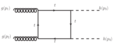
((a))

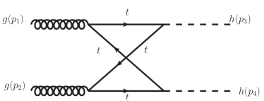
((b))

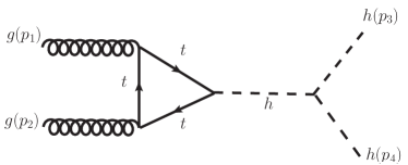
((c))

Figure 1: Feynman diagrams for $gg\rightarrow hh$ in the Standard Model.

II.1 Mixing between $\phi$ and the SM Higgs

After the electroweak symmetry breaking, $h$ and $\phi$ mix through the term, $\mu^{\prime}\left(H^{\dagger}H\right)\phi$. In the $(\phi\quad h)^{T}$ basis, the mass matrix can be written as,

$$M_{\phi h}=\left(\begin{array}[]{c c}M_{\phi}^{2}&\mu^{\prime}v\\ \mu^{\prime}v&m_{h}^{2}\end{array}\right).$$ (9)

We can rotate $(\phi\quad h)^{T}$ to a physical basis $(H_{1}\quad H_{2})^{T}$ as:

$$\left(\begin{array}[]{c}\phi\\ h\end{array}\right)=\left(\begin{array}[]{c c}\cos\theta&\sin\theta\\ -\sin\theta&\cos\theta\end{array}\right)\left(\begin{array}[]{c}H_{1}\\ H_{2}\end{array}\right).$$ (16)

In the new basis, the mass matrix is diagonal and it is defined as,

$$\mathcal{M}_{D}=U^{\dagger}M_{\phi h}U=\left(\begin{array}[]{c c}M^{2}_{H_{1}}&0\\ 0&M^{2}_{H_{2}}\end{array}\right),$$ (19)

where $U$ is an orthogonal rotation matrix and

$$M^{2}_{H_{1}} =M_{\phi}^{2}\cos^{2}\theta+m_{h}^{2}\sin^{2}\theta-\mu^{\prime}v\sin 2\theta,$$ (20)

$$M^{2}_{H_{2}} =M_{\phi}^{2}\sin^{2}\theta+m_{h}^{2}\cos^{2}\theta+\mu^{\prime}v\sin 2\theta.$$ (21)

The mixing angle is given as,

$$\tan 2\theta=\frac{2\mu^{\prime}v}{m_{h}^{2}-M_{\phi}^{2}}.$$ (22)

For a small mixing angle, we can assume $H_{1}$ to be mostly singlet-like while $H_{2}$ will show a strong doublet-like nature. Using Eq. (16), we can recast the important interaction terms as,

$$\lambda vh\left(S^{\dagger}_{1}S_{1}\right)= \ \lambda v(-H_{1}s_{\theta}+H_{2}c_{\theta})\left(S^{\dagger}_{1}S_{1}\right)$$ (23)

$$\lambda^{\prime}\phi\left(S^{\dagger}_{1}S_{1}\right)= \ \lambda^{\prime}(H_{1}c_{\theta}+H_{2}s_{\theta})\left(S^{\dagger}_{1}S_{1}\right)$$ (24)

$$\frac{\mu^{\prime}}{2}h^{2}\phi= \ \frac{\mu^{\prime}}{2}\left(H_{1}H_{2}^{2}c^{3}_{\theta}+H_{2}^{3}c^{2}_{\theta}s_{\theta}\right.$$

$$\quad\quad\left.-2H_{1}H_{2}^{2}s^{2}_{\theta}c_{\theta}+\cdots\right)$$ (25)

where $s_{\theta}=\sin\theta$ and $c_{\theta}=\cos\theta$.

In the subsequent analysis, we assume $c_{\theta}\to 1$ and $s_{\theta}\to 0$. In this limit, we assign $m_{h_{SM}}\simeq M_{H_{2}}=m_{h}$ and $M_{\phi}=M_{H_{1}}$ in the following sections. The above assignment is valid only if $\mu^{\prime}\to 0$ or $M_{\phi}\gg m_{h}>\mu^{\prime}$. In our case, the second condition is applicable as we are primarily interested in a new scalar resonance at $\sim 1.1$ TeV in the di-Higgs production rate.

III Di-Higgs production through a scalar resonance in the LQ model

We first look at the leading-order (LO) SM contributions to the di-Higgs production at the LHC.

III.1 Di-Higgs production in the SM

Here we start with reviewing the dominant production processes for the $gg\to hh$  Eboli:1987dy ; Glover:1987nx ; Plehn:1996wb ; PhysRevD.58.115012 ; Djouadi:1999rca , as shown in Fig. 1. The amplitude for $g^{a\mu}(p_{1})g^{b\nu}(p_{2})\rightarrow h(p_{3})h(p_{4})$ is given by,

$$\mathcal{A}_{ab}^{\mu\nu}=\ \frac{\alpha_{S}\delta_{ab}}{8\pi v^{2}} \Big{[}\mathcal{P}^{\mu\nu}(p_{1},p_{2})\mathcal{F}(\hat{s},\hat{t},\hat{u},m_{t}^{2})$$

$$\ +\mathcal{Q}^{\mu\nu}(p_{1},p_{2},p_{3})\mathcal{G}(\hat{s},\hat{t},\hat{u},m_{t}^{2})\Big{]},$$ (26)

where $a,b$ are the colour indices, $\hat{s},\hat{t},\hat{u}$ are the parton-level Mandelstam variables. The independent tensor projections $\mathcal{P}^{\mu\nu}$ and $\mathcal{Q}^{\mu\nu}$ are defined as,

$$\mathcal{P}^{\mu\nu}= \ g^{\mu\nu}-\frac{p_{1}^{\nu}p_{2}^{\mu}}{p_{1}.p_{2}},$$ (27)

$$\mathcal{Q}^{\mu\nu}= \ g^{\mu\nu}+\frac{2}{\hat{s}p_{T}^{2}}\Big{[}m_{h}^{2}p_{1}^{\nu}p_{2}^{\mu}-2(p_{1}.p_{3})p_{2}^{\mu}p_{3}^{\nu}$$

$$\hskip 48.36958pt-2(p_{2}.p_{3})p_{1}^{\nu}p_{3}^{\mu}+\hat{s}p_{3}^{\mu}p_{3}^{\nu}\Big{]},$$ (28)

where $p_{T}=(\hat{u}\hat{t}-m_{h}^{4})/\hat{s}$ is the transverse momentum of an outgoing Higgs. The triangle diagram contributes only to $\mathcal{F}(\hat{s},\hat{t},\hat{u},m_{t}^{2})$, while box diagrams contribute to both $\mathcal{F}(\hat{s},\hat{t},\hat{u},m_{t}^{2})$ and $\mathcal{G}(\hat{s},\hat{t},\hat{u},m_{t}^{2})$. The triangle diagram has no angular momentum dependence, thus, it is an s-wave contribution. The form factors $\mathcal{F}^{\rm box}$ and $\mathcal{G}^{\rm box}$ can be attributed to the spin-$0$ and spin-$2$ parts of the box amplitude, respectively. The angular dependencies of the form factors by considering the partial wave decomposition of the scattering amplitude are discussed in Refs. Dawson:2012mk ; Borowka:2016ypz . We can split the SM contribution to $\mathcal{F}$ as $\mathcal{F}_{\rm SM}=\mathcal{F}^{\rm tri}_{\rm SM}+\mathcal{F}^{\rm box}_{\rm SM}$ where

$$\mathcal{F}^{\rm tri}_{\rm SM}= \frac{12m_{h}^{2}m_{t}^{2}}{\hat{s}-m_{h}^{2}}\Big{[}2+(4m_{t}^{2}-\hat{s})C_{0}(0,0,\hat{s},m_{t}^{2},m_{t}^{2},m_{t}^{2})\Big{]}$$ (29)

$$\mathcal{F}^{\rm box}_{\rm SM}= -\frac{2m_{t}^{2}}{\hat{s}}\Bigg{[}-4\hat{s}-8m_{t}^{2}\hat{s}C^{00}_{ttt}(\hat{s})-2(4m_{t}^{2}-m_{h}^{2})$$

$$\quad\times\Big{\{}2(m_{h}^{2}-\hat{t})C^{h0}_{ttt}(\hat{t})+2(m_{h}^{2}-\hat{u})C^{h0}_{ttt}(\hat{u})$$

$$\quad-(m_{h}^{4}-\hat{t}\hat{u})D^{h0h0}_{tttt}(\hat{t},\hat{u})\Big{\}}+2m_{t}^{2}\hat{s}(2m_{h}^{2}-8m_{t}^{2}+\hat{s})$$

$$\quad\times\Big{\{}D^{hh00}_{tttt}(\hat{s},\hat{t})+D^{hh00}_{tttt}(\hat{s},\hat{u})+D^{h0h0}_{tttt}(\hat{t},\hat{u})\Big{\}}\Bigg{]}.$$ (30)

Here we have used the following short hands for three-point and four-point functions,

$$C^{ab}_{ijk}(\hat{z})= C_{0}(m^{2}_{a},m^{2}_{b},\hat{z},m^{2}_{i},m^{2}_{j},m^{2}_{k})\quad{\rm and}$$

$$D^{abcd}_{ijkl}(\hat{w},\hat{z})= D_{0}(m_{a}^{2},m_{b}^{2},m_{c}^{2},m_{d}^{2},\hat{w},\hat{z},m_{i}^{2},m_{j}^{2},m_{k}^{2},m_{l}^{2}).$$ (31)

We have ignored all other quark loops except the $t$-quark loop since it gives the dominant contribution. Similarly, $\mathcal{G}_{\rm SM}(\hat{s},\hat{t},\hat{u},m_{t}^{2})$ can be expressed as,

$$\mathcal{G}_{\rm SM}= \frac{2m_{t}^{2}}{m_{h}^{4}-\hat{t}\hat{u}}\Bigg{[}(2m_{h}^{4}-\hat{t}^{2}-\hat{u}^{2})(8m_{t}^{2}-\hat{t}\hat{u})C^{hh}_{ttt}(\hat{s})$$

$$\quad+(m_{h}^{4}-8m_{t}^{2}\hat{t}+\hat{t}^{2})\Big{\{}2(m_{h}^{2}-\hat{t})C^{0h}_{ttt}(\hat{t})-\hat{s}C^{00}_{ttt}(\hat{s})$$

$$\quad+\hat{s}\hat{t}D^{00hh}_{tttt}(\hat{s},\hat{t})\Big{\}}+(m_{h}^{4}-8m_{t}^{2}\hat{u}+\hat{u}^{2})$$

$$\quad\times\Big{\{}2(m_{h}^{2}-\hat{u})C^{0h}_{ttt}(\hat{u})-\hat{s}C^{00}_{ttt}(\hat{s})+\hat{s}\hat{u}D^{00hh}_{tttt}(\hat{s},\hat{u})\Big{\}}$$

$$\quad+2m_{t}^{2}(m_{h}^{4}-\hat{t}\hat{u})(8m_{t}^{2}-\hat{t}-\hat{u})\Big{\{}D^{0h0h}_{tttt}(\hat{t},\hat{u})$$

$$\quad+D^{00hh}_{tttt}(\hat{s},\hat{t})+D^{00hh}_{tttt}(\hat{s},\hat{u})\Big{\}}\Bigg{]}.$$ (32)

As shown, the leading order (LO) amplitude includes the top-quark-mass-dependent terms. The contribution at the next-to-leading order (NLO) in the strong coupling constant both in the infinite top-mass limit and with the full top-mass dependence are considered in Refs. Dawson:1998py ; Alasfar:2019pmn ; Borowka:2016ehy ; Borowka:2016ypz ; Baglio:2018lrj ; Baglio:2020wgt . For higher-order results in different top mass limits, see Refs. Grigo:2014jma ; deFlorian:2013jea ; Grazzini:2018bsd ; Davies:2019nhm ; Davies:2019djw .

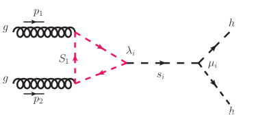
((a))   (a)

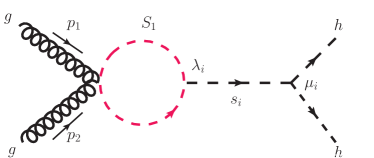
((b))   (b)

Figure 2: Resonance diagrams contributing to $\sigma(gg\rightarrow hh)$.

III.2 The $gg\rightarrow hh$ process in presence of $\phi$

The diagrams for the $gg\rightarrow hh$ through the exchanges of a scalar $s_{i}$ where $s_{i}=\phi,\,h$ are shown in Fig. 2. The complete invariant amplitude for the $gg\rightarrow hh$ processes can be obtained by considering the contributions from both the triangle [Fig. 2(a)] and bubble [Fig. 2(b)] diagrams:

$$\mathcal{A}^{s_{i}}_{gghh}=\frac{\alpha_{S}\delta_{ab}}{8\pi v^{2}}\mathcal{P}^{\mu\nu}(p_{1},p_{2})\mathcal{F}^{s_{i}}_{gghh}.$$ (33)

The loop function in the $gg\,s_{i}$ effective vertex is given by,

$$\mathcal{F}^{s_{i}}_{gghh}=-\frac{\lambda_{i}\mu_{i}v^{2}}{\hat{s}-M_{s_{i}}^{2}}\Big{[}1+2M_{S_{1}}^{2}C_{0}(0,0,\hat{s},M_{S_{1}}^{2},M_{S_{1}}^{2},M_{S_{1}}^{2})\Big{]}.$$ (34)

For the SM Higgs, $\lambda_{i}=\lambda v$ and $\mu_{i}=3m_{h}^{2}/v$, while for the singlet scalar $\phi$, $\lambda_{i}=\lambda^{\prime}$ and $\mu_{i}=\mu^{\prime}/2$. The total $gg\rightarrow hh$ differential cross section including all the resonance channel diagrams (SM+NP) and the box diagrams (SM only) can be calculated as,

$$\frac{d}{d\hat{t}}\hat{\sigma}(gg\rightarrow hh)=\frac{\alpha_{S}^{2}G_{F}^{2}}{2^{14}\pi^{3}\hat{s}^{2}}\Bigg{(}\left|\mathcal{F}+\sum_{s_{i}=h,\phi}\mathcal{F}^{s_{i}}_{gghh}\right|^{2}+\left|\mathcal{G}\right|^{2}\Bigg{)}.$$ (35)

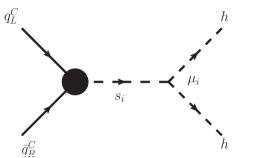
((a))   (a)

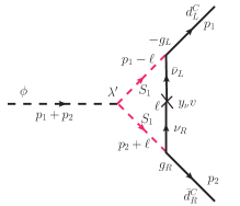
((b))   (b)

Figure 3: (a) Representative Feynman diagram for the $qq\rightarrow hh$ processes and (b) the $q\bar{q}\phi$ vertex.

III.3 The ${qq\rightarrow hh}$ process

Fig. 3(a) shows a generic diagram for the $qq\rightarrow hh$ processes, where $s_{i}=\{\phi,\,h\}$ and $q$ is a down-type quark. The blob represents the $s_{i}q\bar{q}$ effective vertex. The effective couplings are available in Ref. Bhaskar:2020kdr which we repeat below for completeness.

• For $s_{i}=\phi$: For the singlet scalar, there is only one possible vertex, as shown in Fig. 3(b). The corresponding effective coupling is given by,

  $$Y_{q\bar{q}\phi}=-\frac{\mathcal{C}_{q}\lambda^{\prime}v}{16\pi^{2}}\,C_{0}(0,0,\hat{s},M_{\nu_{R}}^{2},M_{S_{1}}^{2},M_{S_{1}}^{2}),$$ (36)

  where we use a compact notation, $\mathcal{C}_{q}=g_{L}g_{R}y_{\nu}$.

• For $s_{i}=h$: For the SM Higgs, there are three possible one loop diagrams along with the tree-level contribution Bhaskar:2020kdr . The total effective coupling for the $q\bar{q}h$ vertex is given by,

  $$Y_{q\bar{q}h}\ = \ \ {y^{\rm SM}_{q}}+\frac{\mathcal{C}_{q}}{16\pi^{2}}\Big{[}B_{0}(0,M_{\nu_{R}}^{2},M_{S_{1}}^{2})-B_{0}(\hat{s},0,M_{\nu_{R}}^{2})$$

  $$\ -M_{S_{1}}^{2}C_{0}(0,0,\hat{s},0,M_{S_{1}}^{2},M_{\nu_{R}}^{2})$$

  $$\ -\lambda v^{2}C_{0}(0,0,\hat{s},M_{S_{1}}^{2},M_{\nu_{R}}^{2},M_{S_{1}}^{2})$$

  $$\ +\frac{\lambda v^{2}}{2}\Big{\{}C_{0}(0,0,\hat{s},0,M_{S_{1}}^{2},M_{\nu_{R}}^{2})$$

  $$\ +M_{S_{1}}^{2}D_{0}(0,0,\hat{s},0,0,0,M_{S_{1}}^{2},M_{S_{1}}^{2},0,M_{\nu_{R}}^{2})$$

  $$\ -C_{0}(0,0,0,M_{S_{1}}^{2},M_{S_{1}}^{2},M_{\nu_{R}}^{2})\Big{\}}\Big{]},$$ (37)

  where $D_{0}$, $C_{0}$ and $B_{0}$ are the Passarino-Veltman four-point, triangle, and bubble integrals, respectively. The ${y^{\rm SM}_{q}}$ term is the SM tree-level contribution.

The differential cross section for $q\bar{q}\rightarrow hh$ at the leading order is given by,

$$\frac{d\hat{\sigma}(q\bar{q}\rightarrow hh)}{dt}=\frac{1}{16\pi}\frac{1}{12\hat{s}}\left|\sum_{s_{i}=h,\phi}\frac{\mu_{i}Y_{q\bar{q}s_{i}}}{\hat{s}-M_{s_{i}}^{2}}\right|^{2}.$$ (38)

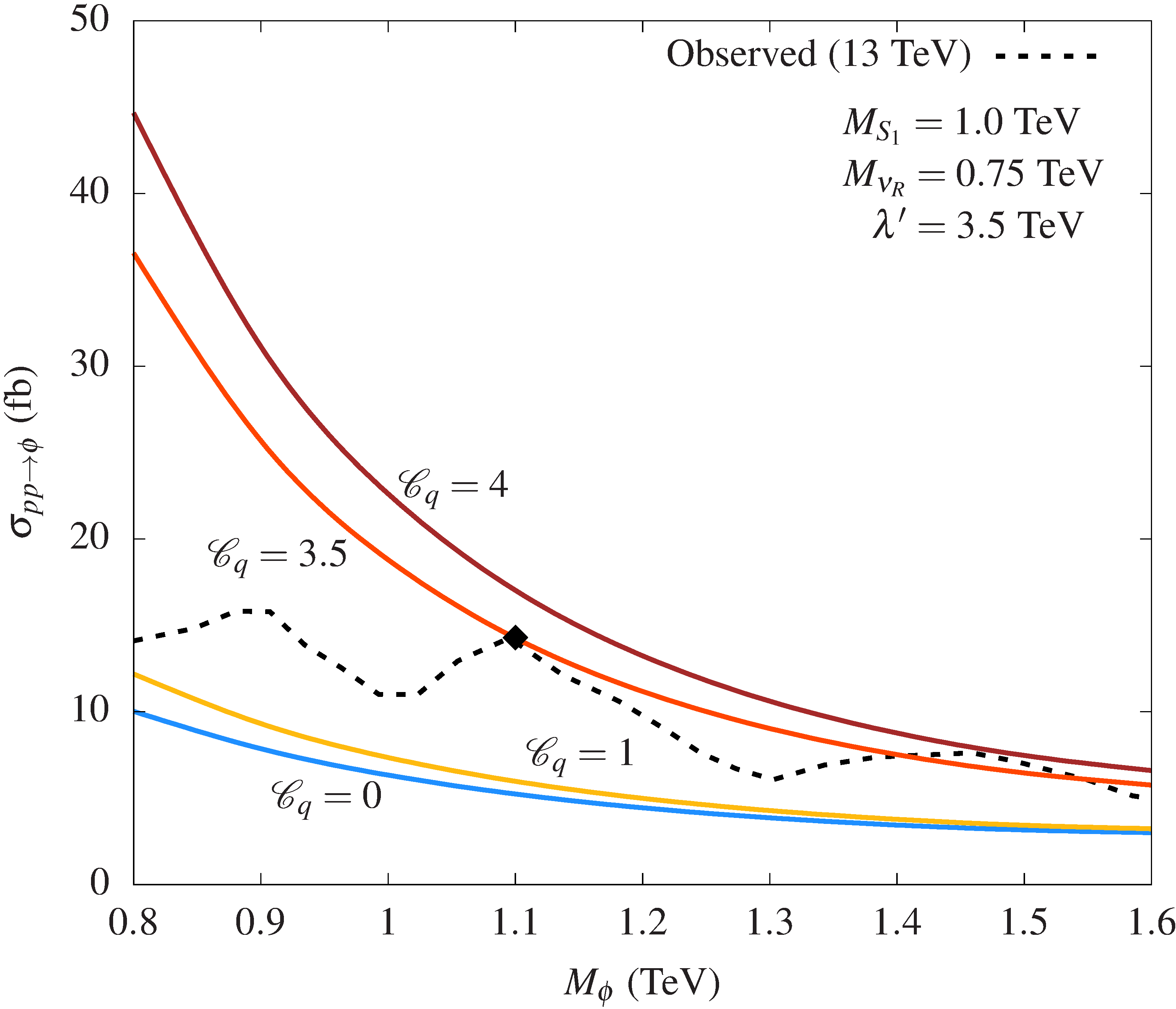
((a))

Figure 4: The $pp\rightarrow\phi$ cross section for different values of $\mathcal{C}_{q}$ as functions of $M_{\phi}$ for $\sqrt{s}=13$ TeV. The combination $\mathcal{C}_{q}=g_{L}g_{R}y_{\nu}$ parametrises the quark contribution. To obtain the cross sections we have used the $14$ TeV di-Higgs K-factors, K${}_{qq~{}(gg)}=1.3~{}(1.72)$, from Ref. Alasfar:2019pmn . Since, BR($\phi\to hh)\approx 1$ in our model, $\sigma(pp\rightarrow\phi)\approx\sigma(pp\rightarrow\phi\to hh)$ [see Eq. (41)]. Hence, we compare it with the upper limit on $\sigma(X\to hh)$ (dashed line) as observed by the ATLAS collaboration in the combined channel ATLAS:2021tyg . The black diamond signifies the parameter choice for which $\sigma(pp\rightarrow\phi)\approx 14.5$ fb at $M_{\phi}=1.1$ TeV.

III.4 The resonant $\mathbb{\phi}$ contribution and choice of parameters

By replacing the $s_{i}$ propagator in Eqs. (34) and (38) by the Breit-Wigner shape,

$$\frac{1}{\hat{s}-M_{s_{i}}^{2}}\to\frac{1}{\hat{s}-M_{s_{i}}^{2}+iM_{s_{i}}\Gamma_{s_{i}}},$$ (39)

we obtain the gluon and quark contributions to the di-Higgs process including the SM-NP interference. However, since we focus on a TeV-range $\phi$, the $\phi$ resonance appears far from the Higgs contribution, making the interference negligible. Hence, in this case, it is possible to look at the resonant $\phi$ contribution separately. This is also justified by the fact that in the parameter range of our interest, the decay width of $\phi$ is quite narrow, $\Gamma_{\phi}/M_{\phi}<1\%$ (for example, for $M_{S_{1}}=1$ TeV, $M_{\nu_{R}}=0.75$ TeV, $\mathcal{C}_{q}=3.5$, $\lambda^{\prime}=3.5$ TeV and $\mu^{\prime}=200$ GeV, we get $\Gamma_{\phi}\lesssim 1$ GeV). As a result, we could use the narrow-width approximation to estimate the resonant $\phi$ contribution to the di-Higgs production. In other words,

$$\sigma^{qq(gg)\to\phi\to hh}_{\rm had}=\sigma^{qq(gg)\rightarrow\phi}_{\rm had}\times{\rm BR}(\phi\rightarrow hh),$$ (40)

where BR stands for branching ratio. For $\mu^{\prime}\gtrsim 100$ GeV, the tree-level decay of $\phi$ dominates, making BR$(\phi\to hh)\approx 1$. We take a conservative $\mu^{\prime}=200$ GeV to keep $\theta$ small. Hence, we can further simplify the above expression as

$$\sigma^{qq(gg)\to\phi\to hh}_{\rm had}\approx\sigma^{qq(gg)\rightarrow\phi}_{\rm had}.$$ (41)

We show $\sigma(pp\to\phi)$ at the $\sqrt{s}=13$ TeV LHC in Fig. 4. The combination $\mathcal{C}_{q}=g_{L}g_{R}y_{\nu}$ parametrises the quark-initiated contribution. The quark contribution switches off for $\mathcal{C}_{q}=0$. Since $\sigma^{qq}$ is proportional to $\mathcal{C}^{2}_{q}$, $\sigma(pp\to\phi)$ increases rapidly with increasing $\mathcal{C}_{q}$. For this plot, we use a benchmark set of parameters, $M_{\nu_{R}}=0.75$ TeV, $M_{S_{1}}=1$ TeV and $\lambda^{\prime}=3.5$ TeV. Our choice of the right-handed neutrino mass is motivated by Ref. ATLAS:2020syg ; ATLAS:2021yij . The current direct search limits on $S_{1}$ lie between $1.7-1.8$ TeV ATLAS:2020dsk . These limits are obtained assuming that the $S_{1}$ decays exclusively to one or two final states (like, e.g., $ej$ or $ej$ and $\nu_{e}j$). However, in our case, the $S_{1}$ can decay to $ue,c\mu,t\tau,d\nu,s\nu,b\nu,d\nu_{R},s\nu_{R},s\nu_{R}$ final states, making the BR in each light mode (i.e., those without $\nu_{R}$—there is no direct limit available from these exotic decay modes) to be less than $1/6$ Bhaskar:2020kdr . As a result, a TeV $S_{1}$ is allowed. Moreover, the combination $\mathcal{C}_{q}=g_{L}g_{R}y_{\nu}$ can be order one even when $g_{L}$ is less than one. Thus, it is possible to take $M_{S_{1}}=1$ TeV and still avoid the constraints from low-energy observables and the single-production searches. Finally, the dimension-one coupling $\lambda^{\prime}$ comes from a NP scale which we assume to be heavier than the entire particle spectrum of our model. The particular choice is motivated by the fact that for $\lambda^{\prime}\sim 3.5$ TeV, $\sigma(pp\to\phi)$ at $13$ TeV fits the small excess seen by ATLAS ATLAS:2021tyg at $M_{\phi}=1.1$ TeV with perturbative couplings.

Background		$\sigma$	QCD
processes		(pb)	order
$V+$ jets  Catani:2009sm ; Balossini:2009sa	$Z+$ jets	$6.33\times 10^{4}$	NNLO
	$W+$ jets	$1.95\times 10^{5}$	NLO
$VV+$ jets Campbell:2011bn	$WW+$ jets	$124.31$	NLO
	$WZ+$ jets	$51.82$	NLO
	$ZZ+$ jets	$17.72$	NLO
Single $t$ Kidonakis:2015nna	$tW$	$83.10$	N2LO
	$tb$	$248.00$	N2LO
	$tj$	$12.35$	N2LO
$tt$ Muselli:2015kba	$tt+$ jets	$988.57$	N3LO
$ttV$ Kulesza:2018tqz	$ttZ$	$1.05$	NLO+NNLL
	$ttW$	$0.65$	NLO+NNLL

Table 1: The significant SM background processes relevant to our signal topology (adapted from Bhaskar:2020gkk ). We used the highest-order QCD cross sections available in the literature for the background processes.

IV LHC phenomenology

To study the prospects of our model at the LHC, we consider the $b\bar{b}\tau^{+}\tau^{-}$ channel where one of the Higgs boson decays to a $b\bar{b}$ pair and the other to a pair of $\tau$’s. We use MadGraph5 Alwall:2014hca to generate the signal and background events at the tree level. We implement the following effective Lagrangian in FeynRules Alloul:2013bka to generate the Universal FeynRules Output Degrande:2011ua model files:

$$\mathcal{L}_{int}\ \supset \ \mu_{h\phi}\left(H^{\dagger}H\right)\phi+\frac{1}{\Lambda_{g}}G_{\mu\nu}^{a}G^{\mu\nu a}\phi+Y_{d\bar{d}\phi}\bar{d}_{L}d_{R}\phi$$

$$\ +Y_{s\bar{s}\phi}\bar{s}_{L}s_{R}\phi+Y_{b\bar{b}\phi}\bar{b}_{L}b_{R}\phi+{\rm H.c}.$$ (42)

where, $\mu_{h\phi}$ and $\Lambda_{g}$ are the dimension-one couplings of the singlet $\phi$ to the SM Higgs and gluons, respectively. To estimate the signal strength for our LHC analysis, we use the K-factors, K${}_{qq~{}(gg)}=1.3~{}(1.72)$ from Ref. Alasfar:2019pmn . We incorporate the higher order corrections to the SM background processes as well. We multiply the LO cross sections with the appropriate QCD $K$-factors known in the literature (see Table 1). We use the NNPDF2.3LO Ball:2012cx parton distribution functions with the default renormalisation and factorisation scales. For showering and hadronisation, these parton level events are passed through Pythia6 Sjostrand:2006za . The detector simulations are performed in Delphes 3.5.0 deFavereau:2013fsa using the Atlas card, incorporating the latest $b$ quark and $\tau$ lepton identification efficiencies ATLAS:2019bwq ; ATLAS:2015xbi . We use the FastJet package Cacciari:2011ma for jet clustering with the anti-$k_{T}$ algorithm Cacciari:2008gp with the radius parameter $R=0.4$.

A simple kinematic-cuts-based analysis is not very promising in this case, as the SM backgrounds are quite significant. Hence, we employ a multivariate analysis that uses Boosted Decision Trees (BDTs) to estimate the signal significance at the HL-LHC.

Figure 5: Pearson’s linear correlation coefficients in the signal for the inputs chosen for BDT analysis.

Parameter	Optimised choice
NTrees	$500$
MinNodeSize	$5.0$%
MaxDepth	$5$
BoostType	AdaBoost
AdaBoostBeta	$0.5$
UseBaggedBoost	True
BaggedSampleFraction	$0.5$
SeparationType	GiniIndex
nCuts	20

Table 2: Summary of optimised BDT hyperparameters.

Feature	Method-unspecific Separation	Feature	Method-specific Ranking
$\Delta R(b_{1},b_{2})$	$0.4968$	$\Delta R(b_{1},b_{2})$	$0.1969$
$\hat{M}_{\phi}$	$0.4209$	$H_{T}$	$0.1601$
$\Delta R(\tau_{h1},\tau_{h2})$	$0.3908$	$\hat{M}_{\phi}$	$0.1302$
$\Delta R(\tau_{h1},b_{2})$	$0.3864$	$m_{T}(b_{1},b_{2})$	$0.1120$
$m_{T}(b_{1},b_{2})$	$0.3386$	$\Delta R(\tau_{h1},\tau_{h2})$	$0.1015$
$\Delta R(\tau_{h2},b_{1})$	$0.3141$	$\Delta R(\tau_{h1},b_{2})$	$0.0913$
$\Delta R(\tau_{h2},b_{2})$	$0.1938$	$\Delta R(\tau_{h1},b_{1})$	$0.0902$
$\Delta R(\tau_{h1},b_{1})$	$0.1287$	$\Delta R(\tau_{h2},b_{1})$	$0.0734$
$H_{T}$	$0.0578$	$\Delta R(\tau_{h2},b_{2})$	$0.0443$

Table 3: Summary of method-unspecific and method-specific ranking for the input features at the benchmark mass point.

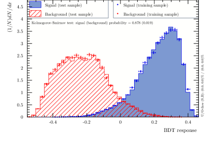
((a))   (a)

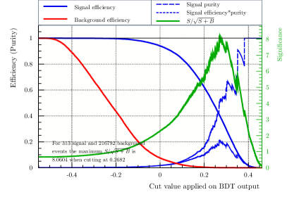
((b))   (b)

Figure 6: BDT Classifier information for $M_{\phi}=1$ TeV: (a) normalised BDT response for the signal and background distributions (training and test samples), (b) classifier cut efficiency as a function of the BDT-cut values.

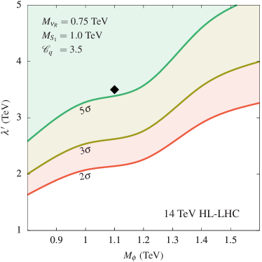
((a))   (a)

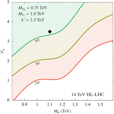
((b))   (b)

Figure 7: HL-LHC ($3$ ab^-1) projection plots: $5\sigma$ (discovery), $3\sigma$ and $2\sigma$ contours in the (a) $M_{\phi}-\lambda^{\prime}$ and (b) $M_{\phi}-\mathcal{C}_{q}$ planes. Regions above the $2\sigma$ ($5\sigma$) lines can be excluded (discovered) at the HL-LHC. The black diamond represents the parameter point marked in Fig. 4: at this point, $\sigma(pp\to\phi)$ in our model fits the slight excess seen by ATLAS ATLAS:2021tyg . At $14$ TeV, it corresponds to a $\phi$ production cross section of about $16.7$ fb.

A multivariate analysis: We generate the process $pp\to\phi\to hh\to b\bar{b}\tau^{+}\tau^{-}$ and select the events with the following event-level criteria:

• Cut-$1$: At least $2$ jets tagged as $\tau_{h}$ leptons (hadronic $\tau$’s)

• Cut-$2$: At least $2$ jets tagged as $b$ quarks

• Cut-$3$: $\Delta\phi(\tau_{h1},b_{1})>2$, i.e. a high $\phi$-separation between the leading-$p_{T}$ $\tau$ lepton and $b$ quark.

These cuts lead to a significant drop in the background events and a moderate drop in the signal events. After these cuts, the efficiencies of quark mediated and gluon mediated signal events are similar ($\approx 4.5\%$). Demanding two $b$ quarks essentially eliminates the $W$ backgrounds. We find that only the $t\bar{t}$ backgrounds remain significant after these cuts. Using the event-level information and the kinematic features of identified objects, we define the following basic set of quantities:

$$H_{T},\hat{M}_{\phi},\,m_{T}(b_{1},b_{2}),\Delta R(\tau_{h1},\tau_{h2}),\,\Delta R(b_{1},b_{2}),$$

$$\Delta R(\tau_{h1},b_{1}),\Delta R(\tau_{h1},b_{2}),\,\Delta R(\tau_{h2},b_{1}),\,\Delta R(\tau_{h2},b_{2})$$ (43)

where $m_{T}(b_{1},b_{2})$ is the transverse mass of the $bb$-system (both transverse and invariant mass of the $bb$-system have similar distributions and are highly correlated, we pick $m_{T}$ since it has slightly better separation visibly), $\Delta R(x,y)$ is the separation between $x$ and $y$ in the $\eta-\phi$ plane, $\hat{M}_{\phi}$ is the estimator of the invariant mass of the singlet $\phi$ constructed from the tagged $\tau_{h}$-leptons and $b$-quarks and $H_{T}$ is the sum of the $p_{T}$ of all jets. We picked these features from a larger set of kinematic variables created from the identified objects after dropping the highly correlated ones (linear correlation $>70\%$ in the signal)—we pick the one with the greatest separation out of a highly co-related pair. The Pearson correlation coefficients between the final set of features are shown in Fig. 5.

We use these features as inputs for the BDT analysis with the adaptive boosting (AdaBoost) optimisation. After obtaining statistically independent event samples for all the signals and background processes considered, we take $30\%$ of the dataset for testing and the rest for training the algorithm. Since there are multiple processes in each of the signal and background classes, we weigh each by the ratio of the expected number of events from the process at the HL-LHC to the number of events fed into the BDT algorithm. We choose the benchmark mass, $M_{\phi}=1$ TeV to optimise the BDT algorithm, which we implement using the TMVA Hocker:2007ht package in ROOT. The Kolmogorov-Smirnov test ensures that the signal and background distributions are well separated—see Fig. 6 for the normalised BDT response and classifier efficiency. The set of optimised BDT hyperparameters are given in Table 2. To show the discriminating power of this set of features in the context of BDTs, we list two measures for each feature: method-unspecific separation and method-specific ranking. The method-unspecific separation which is defined as,

$$\left<S^{2}\right>=\frac{1}{2}\int dy\frac{\left(\hat{y}_{S}\left(y\right)-\hat{y}_{B}\left(y\right)\right)^{2}}{\hat{y}_{S}\left(y\right)+\hat{y}_{B}\left(y\right)}$$ (44)

where $\hat{y}_{S}$ and $\hat{y}_{B}$ are the probability density functions of the signal and background respectively for a particular feature $y$. For signal and background distributions with no overlap, it is unity—features with higher method-unspecific separation values are better at resolving the signal events from the background. Method-specific ranking is derived by counting how often the variables are used to split decision tree nodes, and by weighting each split occurrence by the separation gain-squared it has achieved and by the number of events in the node. We show both these quantities in decreasing order of discriminating power of the features in Table 3. The significance is computed using the formula, $Z=\mathcal{N}_{s}/\sqrt{\mathcal{N}_{s}+\mathcal{N}_{b}}$ where $\mathcal{N}_{s}$ ($\mathcal{N}_{b}$) is the number of signal (background) events surviving at the HL-LHC after the BDT cut. We use the optimised analysis setup to study the collider reach for different masses of $\phi$ in the range $0.8-1.6$ TeV, for the benchmark $\lambda^{\prime}$ and $\mathcal{C}_{q}$. Based on our parametrisation, the number of signal events scales with $\lambda^{\prime}$ and $\mathcal{C}_{q}$ as,

$$\mathcal{N}_{s}=\left(\frac{\lambda^{\prime}}{\rm TeV}\right)^{2}\left(\bar{\mathcal{N}}_{s}^{gg}+\,(\mathcal{C}_{q})^{2}\bar{\mathcal{N}}_{s}^{qq}\right),$$ (45)

where $\bar{\mathcal{N}}_{s}^{gg(qq)}$ is the number of $gg(qq)$-initiated events surviving the BDT cut at $3$ ab^-1 when $\lambda^{\prime}=1$ TeV (and $\mathcal{C}_{q}=1$). We present the $5\sigma$ and $2\sigma$ limits in terms of $\lambda^{\prime}$ and $\mathcal{C}_{q}$ in Fig. 7. One can easily translate these limits in terms of the signal cross section, correcting for the efficiency of each process. We see that for $\mathcal{C}_{q}=3.5$, $\lambda^{\prime}=3.5$ TeV, a $1.1$ TeV $\phi$ (i.e., the parameters to accommodate the current ATLAS excess) can be discovered at the HL-LHC—the signal significance for this point is slightly above $5\sigma$.

V Summary and conclusions

In this letter, we have studied the resonant di-Higgs production mediated by a SM-singlet scalar, $\phi$ at the LHC. In our model, the only SM particle the singlet directly couples to is the Higgs. It couples to $S_{1}$, the charge $-1/3$ weak-singlet scalar Leptoquark, through which it gains an effective coupling with gluon pairs. It also couples to down-type quark-antiquark pairs through loops involving $S_{1}$ and $\nu_{R}$. We showed in an earlier paper Bhaskar:2020kdr that the quark fusion contribution to $\sigma(pp\to\phi)$ could be comparable, or even more significant, than the gluon fusion channel for a suitable choice of parameters. Moreover, since the singlet $\phi$ has tree-level couplings to the Higgs, it dominantly decays to a pair of Higgses. As a result, we have studied an interesting setup where the $\phi$ can be substantially produced at the LHC through both quark and gluon fusion channels and decays to the di-Higgs final state. The parameter ranges for our study were motivated from the ($3.2\sigma$ local significance) excess in the di-Higgs spectrum around $M_{hh}\approx 1.1$ TeV observed by the ATLAS collaboration ATLAS:2021fet ; ATLAS:2021tyg at the $13$ TeV LHC.

We have investigated the prospects of resonant di-Higgs production in our model at the HL-LHC. For this purpose, we have chosen the $b\bar{b}\tau^{+}\tau^{-}$ final state (in which the ATLAS excess was observed ATLAS:2021fet ). To overcome the huge SM background in this channel, we performed a multivariate analysis using Boosted Decision Trees to estimate the signal significance at the HL-LHC. Our study has shown that if we choose the model parameters to account for the excess at the $13$ TeV LHC, the HL-LHC can discover such a resonance. However, there are other variants of multivariate analysis (e.g., BDTs with different boosting techniques, deep-neural-network-based analyses, etc., for e.g. see Adhikary:2020fqf ; Adhikary:2018ise ) that could lead to a better signal yield at the HL-LHC. Moreover, with better $b$- and $\tau$-tagging efficiencies in the future, one could improve this further. A similar study can also be performed in the $bbbb$ mode, which we postpone for a future study. We have presented the results of our study for a wide range of model parameters that can be easily translated to cross sections and, hence, useful for other similar models.

VI Acknowledgments

Our computations were supported in part by SAMKHYA: the High Performance Computing Facility provided by the Institute of Physics (IoP), Bhubaneswar, India. C. N. is supported by the DST-Inspire Fellowship.

References

- (1) O. J. P. Eboli, G. C. Marques, S. F. Novaes and A. A. Natale, TWIN HIGGS BOSON PRODUCTION, Phys. Lett. B 197 (1987) 269–272.
- (2) E. W. N. Glover and J. J. van der Bij, HIGGS BOSON PAIR PRODUCTION VIA GLUON FUSION, Nucl. Phys. B 309 (1988) 282–294.
- (3) T. Plehn, M. Spira and P. M. Zerwas, Pair production of neutral Higgs particles in gluon-gluon collisions, Nucl. Phys. B 479 (1996) 46–64, [hep-ph/9603205]. [Erratum: Nucl.Phys.B 531, 655–655 (1998)].
- (4) S. Dawson, S. Dittmaier and M. Spira, Neutral higgs-boson pair production at hadron colliders: Qcd corrections, Phys. Rev. D 58 (Nov, 1998) 115012.
- (5) A. Djouadi, W. Kilian, M. Muhlleitner and P. M. Zerwas, Production of neutral Higgs boson pairs at LHC, Eur. Phys. J. C 10 (1999) 45–49, [hep-ph/9904287].
- (6) D. de Florian and J. Mazzitelli, Higgs Boson Pair Production at Next-to-Next-to-Leading Order in QCD, Phys. Rev. Lett. 111 (2013) 201801, [1309.6594].
- (7) D. de Florian and J. Mazzitelli, Higgs pair production at next-to-next-to-leading logarithmic accuracy at the LHC, JHEP 09 (2015) 053, [1505.07122].
- (8) S. Borowka, N. Greiner, G. Heinrich, S. P. Jones, M. Kerner, J. Schlenk et al., Higgs Boson Pair Production in Gluon Fusion at Next-to-Leading Order with Full Top-Quark Mass Dependence, Phys. Rev. Lett. 117 (2016) 012001, [1604.06447]. [Erratum: Phys.Rev.Lett. 117, 079901 (2016)].
- (9) S. Borowka, N. Greiner, G. Heinrich, S. P. Jones, M. Kerner, J. Schlenk et al., Full top quark mass dependence in Higgs boson pair production at NLO, JHEP 10 (2016) 107, [1608.04798].
- (10) J. Alison et al., Higgs boson potential at colliders: Status and perspectives, Rev. Phys. 5 (2020) 100045, [1910.00012].
- (11) J. Baglio, F. Campanario, S. Glaus, M. Mühlleitner, M. Spira and J. Streicher, Gluon fusion into Higgs pairs at NLO QCD and the top mass scheme, Eur. Phys. J. C 79 (2019) 459, [1811.05692].
- (12) J. Baglio, F. Campanario, S. Glaus, M. Mühlleitner, J. Ronca and M. Spira, : Combined uncertainties, Phys. Rev. D 103 (2021) 056002, [2008.11626].
- (13) D. de Florian and J. Mazzitelli, Higgs boson pair production at next-to-next-to-leading order in qcd, Phys. Rev. Lett. 111 (Nov, 2013) 201801.
- (14) R. Frederix, S. Frixione, V. Hirschi, F. Maltoni, O. Mattelaer, P. Torrielli et al., Higgs pair production at the LHC with NLO and parton-shower effects, Phys. Lett. B 732 (2014) 142–149, [1401.7340].
- (15) F. Maltoni, E. Vryonidou and M. Zaro, Top-quark mass effects in double and triple Higgs production in gluon-gluon fusion at NLO, JHEP 11 (2014) 079, [1408.6542].
- (16) J. Grigo, K. Melnikov and M. Steinhauser, Virtual corrections to higgs boson pair production in the large top quark mass limit, Nuclear Physics B 888 (2014) 17–29.
- (17) M. Moretti, S. Moretti, F. Piccinini, R. Pittau and A. Polosa, Higgs boson self-couplings at the LHC as a probe of extended higgs sectors, Journal of High Energy Physics 2005 (feb, 2005) 024–024.
- (18) T. Binoth, S. Karg, N. Kauer and R. Rückl, Multi-higgs boson production in the standard model and beyond, Phys. Rev. D 74 (Dec, 2006) 113008.
- (19) D. Y. Shao, C. S. Li, H. T. Li and J. Wang, Threshold resummation effects in Higgs boson pair production at the LHC, JHEP 07 (2013) 169, [1301.1245].
- (20) A. J. Barr, M. J. Dolan, C. Englert and M. Spannowsky, Di-higgs final states augmt2ed – selecting hh events at the high luminosity lhc, Physics Letters B 728 (2014) 308–313.
- (21) V. Barger, L. L. Everett, C. Jackson and G. Shaughnessy, Higgs-pair production and measurement of the triscalar coupling at lhc(8,14), Physics Letters B 728 (2014) 433–436.
- (22) D. E. Ferreira de Lima, A. Papaefstathiou and M. Spannowsky, Standard model Higgs boson pair production in the final state, JHEP 08 (2014) 030, [1404.7139].
- (23) A. Arhrib, R. Benbrik, C.-H. Chen, R. Guedes, and R. Santos, Double neutral higgs production in the two-higgs doublet model at the LHC, Journal of High Energy Physics 2009 (aug, 2009) 035–035.
- (24) J. Baglio, A. Djouadi, R. Gröber, M. M. Mühlleitner, J. Quevillon and M. Spira, The measurement of the Higgs self-coupling at the LHC: theoretical status, JHEP 04 (2013) 151, [1212.5581].
- (25) M. J. Dolan, C. Englert and M. Spannowsky, New physics in lhc higgs boson pair production, Phys. Rev. D 87 (Mar, 2013) 055002.
- (26) C. Han, X. Ji, L. Wu, P. Wu and J. M. Yang, Higgs pair production with SUSY QCD correction: revisited under current experimental constraints, JHEP 04 (2014) 003, [1307.3790].
- (27) F. Goertz, A. Papaefstathiou, L. L. Yang and J. Zurita, Higgs boson pair production in the D=6 extension of the SM, JHEP 04 (2015) 167, [1410.3471].
- (28) D. A. Dicus, C. Kao and W. W. Repko, Interference effects and the use of Higgs boson pair production to study the Higgs trilinear self coupling, Phys. Rev. D 92 (2015) 093003, [1504.02334].
- (29) C. Delaunay, C. Grojean and G. Perez, Modified Higgs Physics from Composite Light Flavors, JHEP 09 (2013) 090, [1303.5701].
- (30) C.-Y. Chen, S. Dawson and I. M. Lewis, Top partners and higgs boson production, Phys. Rev. D 90 (Aug, 2014) 035016.
- (31) A. Azatov, R. Contino, G. Panico and M. Son, Effective field theory analysis of double Higgs boson production via gluon fusion, Phys. Rev. D 92 (2015) 035001, [1502.00539].
- (32) R. Contino, M. Ghezzi, M. Moretti, G. Panico, F. Piccinini and A. Wulzer, Anomalous Couplings in Double Higgs Production, JHEP 08 (2012) 154, [1205.5444].
- (33) M. Gillioz, R. Grober, C. Grojean, M. Muhlleitner and E. Salvioni, Higgs Low-Energy Theorem (and its corrections) in Composite Models, JHEP 10 (2012) 004, [1206.7120].
- (34) N. Liu, S. Hu, B. Yang and J. Han, Impact of top-Higgs couplings on Di-Higgs production at future colliders, JHEP 01 (2015) 008, [1408.4191].
- (35) N. D. Christensen, T. Han, Z. Liu and S. Su, Low-Mass Higgs Bosons in the NMSSM and Their LHC Implications, JHEP 08 (2013) 019, [1303.2113].
- (36) M. Gouzevitch, A. Oliveira, J. Rojo, R. Rosenfeld, G. P. Salam and V. Sanz, Scale-invariant resonance tagging in multijet events and new physics in Higgs pair production, JHEP 07 (2013) 148, [1303.6636].
- (37) J. Liu, X.-P. Wang and S.-h. Zhu, Discovering extra Higgs boson via pair production of the SM-like Higgs bosons, 1310.3634.
- (38) J. M. No and M. Ramsey-Musolf, Probing the higgs portal at the lhc through resonant di-higgs production, Phys. Rev. D 89 (May, 2014) 095031.
- (39) J. Baglio, O. Eberhardt, U. Nierste and M. Wiebusch, Benchmarks for higgs boson pair production and heavy higgs boson searches in the two-higgs-doublet model of type ii, Phys. Rev. D 90 (Jul, 2014) 015008.
- (40) N. Kumar and S. P. Martin, Lhc search for di-higgs decays of stoponium and other scalars in events with two photons and two bottom jets, Phys. Rev. D 90 (Sep, 2014) 055007.
- (41) B. Hespel, D. Lopez-Val and E. Vryonidou, Higgs pair production via gluon fusion in the Two-Higgs-Doublet Model, JHEP 09 (2014) 124, [1407.0281].
- (42) V. Barger, L. L. Everett, C. B. Jackson, A. D. Peterson and G. Shaughnessy, New physics in resonant production of higgs boson pairs, Phys. Rev. Lett. 114 (Jan, 2015) 011801.
- (43) C.-Y. Chen, S. Dawson and I. M. Lewis, Exploring resonant di-Higgs boson production in the Higgs singlet model, Phys. Rev. D 91 (2015) 035015, [1410.5488].
- (44) M. van Beekveld, W. Beenakker, S. Caron, R. Castelijn, M. Lanfermann and A. Struebig, Higgs, di-Higgs and tri-Higgs production via SUSY processes at the LHC with 14 TeV, JHEP 05 (2015) 044, [1501.02145].
- (45) U. Ellwanger and A. M. Teixeira, Excessive Higgs pair production with little MET from squarks and gluinos in the NMSSM, JHEP 04 (2015) 172, [1412.6394].
- (46) A. Belyaev, M. Drees, O. J. P. Éboli, J. K. Mizukoshi and S. F. Novaes, Supersymmetric higgs boson pair production at hadron colliders, Phys. Rev. D 60 (Sep, 1999) 075008.
- (47) A. A. Barrientos Bendezú and B. A. Kniehl, Pair production of neutral higgs bosons at the cern large hadron collider, Phys. Rev. D 64 (Jul, 2001) 035006.
- (48) E. Asakawa, D. Harada, S. Kanemura, Y. Okada and K. Tsumura, Higgs boson pair production in new physics models at hadron, lepton, and photon colliders, Phys. Rev. D 82 (Dec, 2010) 115002.
- (49) G. D. Kribs and A. Martin, Enhanced di-higgs production through light colored scalars, Phys. Rev. D 86 (Nov, 2012) 095023.
- (50) S. Dawson, A. Ismail and I. Low, What’s in the loop? The anatomy of double Higgs production, Phys. Rev. D 91 (2015) 115008, [1504.05596].
- (51) T. Enkhbat, Scalar leptoquarks and Higgs pair production at the LHC, JHEP 01 (2014) 158, [1311.4445].
- (52) J.-J. Liu, W.-G. Ma, G. Li, R.-Y. Zhang and H.-S. Hou, Higgs boson pair production in the little Higgs model at hadron collider, Phys. Rev. D 70 (2004) 015001, [hep-ph/0404171].
- (53) C. O. Dib, R. Rosenfeld and A. Zerwekh, Double Higgs production and quadratic divergence cancellation in little Higgs models with T parity, JHEP 05 (2006) 074, [hep-ph/0509179].
- (54) C.-R. Chen and I. Low, Double take on new physics in double Higgs boson production, Phys. Rev. D 90 (2014) 013018, [1405.7040].
- (55) A. Pierce, J. Thaler and L.-T. Wang, Disentangling dimension six operators through di-higgs boson production, Journal of High Energy Physics 2007 (may, 2007) 070–070.
- (56) W. Ma, C.-X. Yue and Y.-Z. Wang, Pair production of neutral higgs bosons from the left-right twin higgs model at the ilc and lhc, Phys. Rev. D 79 (May, 2009) 095010.
- (57) X.-F. Han, L. Wang and J. M. Yang, Higgs-pair production and decay in simplest little higgs model, Nuclear Physics B 825 (2010) 222–230.
- (58) S. Dawson, E. Furlan and I. Lewis, Unravelling an extended quark sector through multiple higgs production?, Phys. Rev. D 87 (Jan, 2013) 014007.
- (59) L. Edelhäuser, A. Knochel and T. Steeger, Applying EFT to Higgs Pair Production in Universal Extra Dimensions, JHEP 11 (2015) 062, [1503.05078].
- (60) I. M. Lewis and M. Sullivan, Benchmarks for Double Higgs Production in the Singlet Extended Standard Model at the LHC, Phys. Rev. D 96 (2017) 035037, [1701.08774].
- (61) P. Huang, A. Joglekar, M. Li and C. E. M. Wagner, Corrections to di-Higgs boson production with light stops and modified Higgs couplings, Phys. Rev. D 97 (2018) 075001, [1711.05743].
- (62) L. Alasfar, R. Corral Lopez and R. Gröber, Probing Higgs couplings to light quarks via Higgs pair production, JHEP 11 (2019) 088, [1909.05279].
- (63) L. Da Rold, M. Epele, A. Medina, N. I. Mileo and A. Szynkman, Enhancement of the double Higgs production via leptoquarks at the LHC, JHEP 08 (2021) 100, [2105.06309].
- (64) U. Baur, T. Plehn and D. L. Rainwater, Probing the Higgs selfcoupling at hadron colliders using rare decays, Phys. Rev. D 69 (2004) 053004, [hep-ph/0310056].
- (65) F. Kling, T. Plehn and P. Schichtel, Maximizing the significance in Higgs boson pair analyses, Phys. Rev. D 95 (2017) 035026, [1607.07441].
- (66) V. Barger, L. L. Everett, C. B. Jackson and G. Shaughnessy, Higgs-Pair Production and Measurement of the Triscalar Coupling at LHC(8,14), Phys. Lett. B 728 (2014) 433–436, [1311.2931].
- (67) C.-T. Lu, J. Chang, K. Cheung and J. S. Lee, An exploratory study of Higgs-boson pair production, JHEP 08 (2015) 133, [1505.00957].
- (68) A. Adhikary, S. Banerjee, R. K. Barman, B. Bhattacherjee and S. Niyogi, Revisiting the non-resonant Higgs pair production at the HL-LHC, JHEP 07 (2018) 116, [1712.05346].
- (69) A. Alves, T. Ghosh and K. Sinha, Can We Discover Double Higgs Production at the LHC?, Phys. Rev. D 96 (2017) 035022, [1704.07395].
- (70) J. Chang, K. Cheung, J. S. Lee, C.-T. Lu and J. Park, Higgs-boson-pair production H()H() from gluon fusion at the HL-LHC and HL-100 TeV hadron collider, Phys. Rev. D 100 (2019) 096001, [1804.07130].
- (71) M. J. Dolan, C. Englert and M. Spannowsky, Higgs self-coupling measurements at the LHC, JHEP 10 (2012) 112, [1206.5001].
- (72) J. K. Behr, D. Bortoletto, J. A. Frost, N. P. Hartland, C. Issever and J. Rojo, Boosting Higgs pair production in the final state with multivariate techniques, Eur. Phys. J. C 76 (2016) 386, [1512.08928].
- (73) D. Wardrope, E. Jansen, N. Konstantinidis, B. Cooper, R. Falla and N. Norjoharuddeen, Non-resonant Higgs-pair production in the final state at the LHC, Eur. Phys. J. C 75 (2015) 219, [1410.2794].
- (74) H. Abouabid, A. Arhrib, D. Azevedo, J. E. Falaki, P. M. Ferreira, M. Mühlleitner et al., Benchmarking Di-Higgs Production in Various Extended Higgs Sector Models, 2112.12515.
- (75) J. Cao, Z. Heng, L. Shang, P. Wan and J. M. Yang, Pair Production of a 125 GeV Higgs Boson in MSSM and NMSSM at the LHC, JHEP 04 (2013) 134, [1301.6437].
- (76) J. Cao, D. Li, L. Shang, P. Wu and Y. Zhang, Exploring the Higgs Sector of a Most Natural NMSSM and its Prediction on Higgs Pair Production at the LHC, JHEP 12 (2014) 026, [1409.8431].
- (77) P. Huang and Y. H. Ng, Di-Higgs Production in SUSY models at the LHC, Eur. Phys. J. Plus 135 (2020) 660, [1910.13968].
- (78) G. D. Kribs and A. Martin, Enhanced di-Higgs Production through Light Colored Scalars, Phys. Rev. D 86 (2012) 095023, [1207.4496].
- (79) D. Egana-Ugrinovic, S. Homiller and P. Meade, Multi-Higgs Production Probes Higgs Flavor, Phys. Rev. D 103 (2021) 115005, [2101.04119].
- (80) P. Agrawal and U. Mahanta, Leptoquark contribution to the Higgs boson production at the CERN LHC collider, Phys. Rev. D61 (2000) 077701, [hep-ph/9911497].
- (81) A. Bhaskar, D. Das, B. De and S. Mitra, Enhancing scalar productions with leptoquarks at the LHC, Phys. Rev. D 102 (2020) 035002, [2002.12571].
- (82) I. Dors̆ner, S. Fajfer, A. Greljo, J. F. Kamenik and N. Kos̆nik, Physics of leptoquarks in precision experiments and at particle colliders, Phys. Rept. 641 (2016) 1–68, [1603.04993].
- (83) T. Mandal, S. Mitra and S. Seth, Pair Production of Scalar Leptoquarks at the LHC to NLO Parton Shower Accuracy, Phys. Rev. D93 (2016) 035018, [1506.07369].
- (84) D. Das, K. Ghosh, M. Mitra and S. Mondal, Probing sterile neutrinos in the framework of inverse seesaw mechanism through leptoquark productions, Phys. Rev. D97 (2018) 015024, [1708.06206].
- (85) I. Doršner, S. Fajfer, D. A. Faroughy and N. Košnik, The role of the GUT leptoquark in flavor universality and collider searches, 1706.07779. [JHEP10,188(2017)].
- (86) P. Bandyopadhyay and R. Mandal, Revisiting scalar leptoquark at the LHC, Eur. Phys. J. C78 (2018) 491, [1801.04253].
- (87) G. Hiller, D. Loose and I. Nišandžić, Flavorful leptoquarks at hadron colliders, Phys. Rev. D97 (2018) 075004, [1801.09399].
- (88) A. Biswas, A. Shaw and A. K. Swain, Collider signature of Leptoquark with flavour observables, LHEP 2 (2019) 126, [1811.08887].
- (89) T. Mandal, S. Mitra and S. Raz, motivated leptoquark scenarios: Impact of interference on the exclusion limits from LHC data, Phys. Rev. D99 (2019) 055028, [1811.03561].
- (90) T. Faber, Y. Liu, W. Porod, M. Hudec, M. Malinský, F. Staub et al., Collider phenomenology of a unified leptoquark model, 1812.07592.
- (91) A. Alves, O. J. P. Eboli, G. Grilli Di Cortona and R. R. Moreira, Indirect and monojet constraints on scalar leptoquarks, Phys. Rev. D99 (2019) 095005, [1812.08632].
- (92) U. Aydemir, T. Mandal and S. Mitra, Addressing the anomalies with an leptoquark from grand unification, Phys. Rev. D101 (2020) 015011, [1902.08108].
- (93) K. Chandak, T. Mandal and S. Mitra, Hunting for scalar leptoquarks with boosted tops and light leptons, Phys. Rev. D100 (2019) 075019, [1907.11194].
- (94) R. Padhan, S. Mandal, M. Mitra and N. Sinha, Signatures of class of Leptoquarks at the upcoming colliders, Phys. Rev. D 101 (2020) 075037, [1912.07236].
- (95) B. C. Allanach, T. Corbett and M. Madigan, Sensitivity of Future Hadron Colliders to Leptoquark Pair Production in the Di-Muon Di-Jets Channel, Eur. Phys. J. C 80 (2020) 170, [1911.04455].
- (96) A. Bhaskar, D. Das, T. Mandal, S. Mitra and C. Neeraj, Precise limits on the charge-2/3 U1 vector leptoquark, Phys. Rev. D 104 (2021) 035016, [2101.12069].
- (97) A. Bhaskar, T. Mandal, S. Mitra and M. Sharma, Improving third-generation leptoquark searches with combined signals and boosted top quarks, Phys. Rev. D 104 (2021) 075037, [2106.07605].
- (98) T. Mandal, S. Mitra and S. Seth, Single Productions of Colored Particles at the LHC: An Example with Scalar Leptoquarks, JHEP 07 (2015) 028, [1503.04689].
- (99) ATLAS collaboration, Search for resonant and non-resonant Higgs boson pair production in the decay channel using 13 TeV collision data from the ATLAS detector, ATLAS-CONF-2021-030, 2021.
- (100) ATLAS collaboration, Combination of searches for non-resonant and resonant Higgs boson pair production in the , and decay channels using collisions at = 13 TeV with the ATLAS detector, ATLAS-CONF-2021-052, 2021.
- (101) CMS collaboration, A. M. Sirunyan et al., Combination of searches for Higgs boson pair production in proton-proton collisions at 13 TeV, Phys. Rev. Lett. 122 (2019) 121803, [1811.09689].
- (102) CMS collaboration, A. Tumasyan et al., Search for heavy resonances decaying to a pair of Lorentz-boosted Higgs bosons in final states with leptons and a bottom quark pair at = 13 TeV, 2112.03161.
- (103) R. Mandal and A. Pich, Constraints on scalar leptoquarks from lepton and kaon physics, JHEP 12 (2019) 089, [1908.11155].
- (104) S. Dawson, E. Furlan and I. Lewis, Unravelling an extended quark sector through multiple Higgs production?, Phys. Rev. D 87 (2013) 014007, [1210.6663].
- (105) S. Dawson, S. Dittmaier and M. Spira, Neutral Higgs boson pair production at hadron colliders: QCD corrections, Phys. Rev. D 58 (1998) 115012, [hep-ph/9805244].
- (106) J. Grigo, K. Melnikov and M. Steinhauser, Virtual corrections to Higgs boson pair production in the large top quark mass limit, Nucl. Phys. B 888 (2014) 17–29, [1408.2422].
- (107) M. Grazzini, G. Heinrich, S. Jones, S. Kallweit, M. Kerner, J. M. Lindert et al., Higgs boson pair production at NNLO with top quark mass effects, JHEP 05 (2018) 059, [1803.02463].
- (108) J. Davies, R. Gröber, A. Maier, T. Rauh and M. Steinhauser, Top quark mass dependence of the Higgs boson-gluon form factor at three loops, Phys. Rev. D 100 (2019) 034017, [1906.00982]. [Erratum: Phys.Rev.D 102, 059901 (2020)].
- (109) J. Davies and M. Steinhauser, Three-loop form factors for Higgs boson pair production in the large top mass limit, JHEP 10 (2019) 166, [1909.01361].
- (110) ATLAS collaboration, G. Aad et al., Search for squarks and gluinos in final states with jets and missing transverse momentum using 139 fb-1 of =13 TeV collision data with the ATLAS detector, JHEP 02 (2021) 143, [2010.14293].
- (111) ATLAS collaboration, G. Aad et al., Search for new phenomena in final states with -jets and missing transverse momentum in TeV collisions with the ATLAS detector, JHEP 05 (2021) 093, [2101.12527].
- (112) ATLAS collaboration, G. Aad et al., Search for pairs of scalar leptoquarks decaying into quarks and electrons or muons in = 13 TeV collisions with the ATLAS detector, JHEP 10 (2020) 112, [2006.05872].
- (113) S. Catani, L. Cieri, G. Ferrera, D. de Florian and M. Grazzini, Vector boson production at hadron colliders: a fully exclusive QCD calculation at NNLO, Phys. Rev. Lett. 103 (2009) 082001, [0903.2120].
- (114) G. Balossini, G. Montagna, C. M. Carloni Calame, M. Moretti, O. Nicrosini, F. Piccinini et al., Combination of electroweak and QCD corrections to single W production at the Fermilab Tevatron and the CERN LHC, JHEP 01 (2010) 013, [0907.0276].
- (115) J. M. Campbell, R. K. Ellis and C. Williams, Vector boson pair production at the LHC, JHEP 07 (2011) 018, [1105.0020].
- (116) N. Kidonakis, Theoretical results for electroweak-boson and single-top production, PoS DIS2015 (2015) 170, [1506.04072].
- (117) C. Muselli, M. Bonvini, S. Forte, S. Marzani and G. Ridolfi, Top Quark Pair Production beyond NNLO, JHEP 08 (2015) 076, [1505.02006].
- (118) A. Kulesza, L. Motyka, D. Schwartländer, T. Stebel and V. Theeuwes, Associated production of a top quark pair with a heavy electroweak gauge boson at NLONNLL accuracy, Eur. Phys. J. C79 (2019) 249, [1812.08622].
- (119) A. Bhaskar, T. Mandal and S. Mitra, Boosting vector leptoquark searches with boosted tops, Phys. Rev. D 101 (2020) 115015, [2004.01096].
- (120) J. Alwall, R. Frederix, S. Frixione, V. Hirschi, F. Maltoni, O. Mattelaer et al., The automated computation of tree-level and next-to-leading order differential cross sections, and their matching to parton shower simulations, JHEP 07 (2014) 079, [1405.0301].
- (121) A. Alloul, N. D. Christensen, C. Degrande, C. Duhr and B. Fuks, FeynRules 2.0 - A complete toolbox for tree-level phenomenology, Comput. Phys. Commun. 185 (2014) 2250–2300, [1310.1921].
- (122) C. Degrande, C. Duhr, B. Fuks, D. Grellscheid, O. Mattelaer and T. Reiter, UFO - The Universal FeynRules Output, Comput. Phys. Commun. 183 (2012) 1201–1214, [1108.2040].
- (123) R. D. Ball et al., Parton distributions with LHC data, Nucl. Phys. B867 (2013) 244–289, [1207.1303].
- (124) T. Sjostrand, S. Mrenna and P. Z. Skands, PYTHIA 6.4 Physics and Manual, JHEP 05 (2006) 026, [hep-ph/0603175].
- (125) DELPHES 3 collaboration, J. de Favereau, C. Delaere, P. Demin, A. Giammanco, V. Lemaître, A. Mertens et al., DELPHES 3, A modular framework for fast simulation of a generic collider experiment, JHEP 02 (2014) 057, [1307.6346].
- (126) ATLAS collaboration, G. Aad et al., ATLAS b-jet identification performance and efficiency measurement with events in pp collisions at TeV, Eur. Phys. J. C 79 (2019) 970, [1907.05120].
- (127) ATLAS collaboration, Reconstruction, Energy Calibration, and Identification of Hadronically Decaying Tau Leptons in the ATLAS Experiment for Run-2 of the LHC, .
- (128) M. Cacciari, G. P. Salam and G. Soyez, FastJet User Manual, Eur. Phys. J. C72 (2012) 1896, [1111.6097].
- (129) M. Cacciari, G. P. Salam and G. Soyez, The anti- jet clustering algorithm, JHEP 04 (2008) 063, [0802.1189].
- (130) A. Hocker et al., TMVA - Toolkit for Multivariate Data Analysis, physics/0703039.
- (131) A. Adhikary, R. K. Barman and B. Bhattacherjee, Prospects of non-resonant di-Higgs searches and Higgs boson self-coupling measurement at the HE-LHC using machine learning techniques, JHEP 12 (2020) 179, [2006.11879].
- (132) A. Adhikary, S. Banerjee, R. Kumar Barman and B. Bhattacherjee, Resonant heavy Higgs searches at the HL-LHC, JHEP 09 (2019) 068, [1812.05640].