Fermions on Quantum Geometry and Resolution of Doubling Problem

Abstract

The fermion doubling problem has an important impact on quantum gravity, by revealing the tension between fermion and the fundamental discreteness of quantum spacetime. In this work, we discover that in Loop Quantum Gravity, the quantum geometry involving superposition of states associated with lattice refinements provides a resolution to the fermion doubling problem. We construct and analyze the fermion propagator on the quantum geometry, and we show that all fermion doubler modes are suppressed in the propagator. Our result suggests that the superposition nature of quantum geometry should resolve the tension between fermion and the fundamental discreteness, and relate to the continuum limit of quantum gravity.

The physical world is made of gravity and matters. The quantum theory of matters has been well-developed by the standard model, where gravity is, however, classical. It has been suggested that a consistent theory of gravity coupled to quantized matter should also have the gravitational field quantized Page and Geilker (1981). On the other hand, Quantum Gravity (QG) also needs matter couplings, not only because matter fields are dominant in the universe, but also due to the universal gravity-matter interaction, which makes matters serve as probes for empirically testing QG effects. The matter couplings provide a toolbox for early studies of the ultraviolet (UV) behavior of QG Deser and van Nieuwenhuizen (1974); ’t Hooft and Veltman (1974); Goroff and Sagnotti (1986), and play important roles in cosmology, black holes, asymptotic safety, QG phenomenology, etc Ashtekar et al. (2021); Hawking (1975); Donà et al. (2014); Perez and Sudarsky (2019).

Loop Quantum Gravity (LQG) is a promising candidate for the background-independent and non-perturbative QG. Matter couplings in LQG have been extensively explored (see e.g. Ashtekar et al. (1989); Thiemann (1998a); Sahlmann and Thiemann (2006); Lewandowski and Zhang (2021); Bodendorfer et al. (2013); Bojowald and Das (2008); Domagala et al. (2010); Kisielowski and Lewandowski (2019); Bianchi et al. (2013); Oriti and Ryan (2006); Mansuroglu and Sahlmann (2021); Zhang and Ma (2011); Kamiński et al. (2006)). A framework of coupling standard model to LQG is developed with the interesting feature of the ultraviolet regularity Thiemann (1998a).

This work focuses on chiral fermions in LQG. Due to the fundamental discreteness of LQG, the fermion coupling resembles the Lattice Field Theory (LFT) to some extent, on any given discrete spacetime in LQG. It is well-known that chiral fermions in LFT suffers the doubling problem, i.e. each fermion results in $2^{m}$ fermion species on $m$-dimensional lattice Montvay and Münster (1994); Nielsen and Ninomiya (1981). This fact leads to the suspicion of the fermion doubling problem in LQG Barnett and Smolin (2015). However, there also exists the opposite opinion arguing that the fermion doubling problem may not exist in LQG due to the superposition of quantum geometries Gambini and Pullin (2015); Bianchi et al. (2013); Han and Rovelli (2013). The confusion on fermion doubling has been long-standing in the LQG community since the first paper on LQG-fermion in 1997. The similar issue should exist in all QG approaches with discrete spacetimes. This issue is crucial because it reveals the tension between fermion and the fundamental discreteness of quantum spacetime, given that the fundamental discreteness is believed to be a key feature of QG ’t Hooft (2016); Wheeler (1955); Hawking (1978).

A resolution of this tension is proposed in this paper from the perspective of LQG. We construct and compute the chiral fermion propagator of LQG. Due to the superposition of lattices given by the quantum geometry in LQG, the resulting propagator averages the lattice fermion propagators over a sequence of lattice refinements. We show that the average results in suppression of all fermion doubling modes, while the physical mode is kept unchanged. Our result implies that the LQG fermion propagator has the correct continuum limit, and suggests the nature of superposition in quantum geometries be the key to resolve the tension between fermion and the fundamental discreteness. Our result also provides an interesting example for understanding the continuum limit of LQG.

Fermion doubling and a resolution.— Let us firstly consider LFT on 4d Minkowski spacetime, where the time is continuous and the space is discretized by a cubic lattice $\gamma$ Kogut and Susskind (1975); Creutz et al. (2002). The propagator of chiral fermion has the following expression:

$$G_{\omega,\vec{k}}(\gamma,a)=\frac{-\omega\mathbf{1}_{2\times 2}+\frac{1}{a}\sum_{I=1}^{3}\bm{\sigma}^{I}\sin\left(ak_{I}\right)}{\omega^{2}-\frac{1}{a^{2}}\sum_{I=1}^{3}\sin^{2}\left(ak_{I}\right)+i\epsilon}$$ (1)

where $I=1,2,3$ labels the directions on $\gamma$. $a$ is the lattice spacing, and $\epsilon$ is the Feynman regulator. $G_{\omega,\vec{k}}(\gamma,a)$ is a $2\times 2$ matrix whose matrix indices are Weyl spinor indices, denoted by $A,B=\pm$. The range of momentum $k^{I}$ is the fundamental Brillouin zone (FBZ) $-\pi/a\leq k^{I}<\pi/a$. $G_{\omega,\vec{k}}(\gamma,a)$ has the doubling problem: A physical pole at e.g. $(\omega,\vec{k})=(\omega,k,0,0)$ (satisfying $\omega=\frac{1}{a^{2}}\sin\left(ak\right)>0$) implies another spurious doubler pole at $(\omega,\frac{\pi}{a}-k,0,0)$, so the fermion species is doubled in each direction on the lattice. The fermion doubling problem causes the trouble of the continuum limit of fermions on the lattice, and is intractably linked to chirality by the Nielsen-Ninomiya no-go theorem Nielsen and Ninomiya (1981).

LQG gives quantum geometry states as superposition of lattices, and it indicates a resolution to the doubling problem by taking into account the average of the propagators over the refinements of the lattice. Namely we consider the following quantity, whose derivation from LQG is given in a moment

$${G}_{\omega,\vec{k}}=\frac{1}{L}\sum_{n=1}^{L}\chi_{n,\vec{k}}G_{\omega,\vec{k}}\left(\gamma_{n},a_{n}\right),$$ (2)

where $L$ is large and $\gamma_{n}$ are refinements of $\gamma_{1}=\gamma$ and has the spacing $a_{n}=a_{1}/n$ (see FIG.1). We introduce the short-hand notation $\mathrm{FBZ}(\gamma_{n})\equiv[-\pi/a_{n},\pi/a_{n})^{3}$ for the FBZ on $\gamma_{n}$ with the spacing $a_{n}$, and we have $\mathrm{FBZ}(\gamma_{n})\subset\mathrm{FBZ}(\gamma_{n+1})$. $\chi_{n,\vec{k}}=1$ if $\vec{k}$ belongs to $\mathrm{FBZ}(\gamma_{n})$, otherwise $\chi_{n,k}=0$.

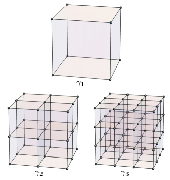
Figure 1: Lattice refinement of a cell of $\gamma_{1}$, to $\gamma_{2}$ and $\gamma_{3}$. Along each direction on $\gamma_{n}$, the number of vertices $N_{n}$ satisfies $N_{n}=nN_{1}$.

The assumptions of Nielsen-Ninomiya theorem is clearly violated by summing over lattices. Although apparently (2) adds to ${G}_{\omega,\vec{k}}$ the spurious doubler poles from all $\gamma_{n}$, the contribution from each doubler pole are suppressed, thanks to the refinement and averaging. To explain the mechanism, we firstly note that for $\epsilon>0$, the poles of ${G}_{\omega,\vec{k}}$ are away from real $(\omega,\vec{k})$-space, so ${G}_{\omega,\vec{k}}$ is finite for real $(\omega,\vec{k})$’s. Given an $\omega_{o}>0$ such that the physical mode, e.g. $\vec{k}_{o}=(k_{o},0,0)$, is in $\mathrm{FBZ}(\gamma_{1})$, and assuming $a_{1}$ is sufficiently small so that $k_{o}\simeq\omega_{o}$, $(\omega_{o},\vec{k}_{o})$ is close to a pole of every $G_{\omega,\vec{k}}\left(\gamma_{n},a_{n}\right)$ and gives equally large contributions to all terms in (2), while the contributions are averaged over $\{\gamma_{n}\}$. In contrast, each doubler mode $\vec{k}_{n}=({\pi}/{a_{n}}-k_{o},0,0)$ associated to $\gamma_{n}$ only gives a single large contribution to the $n$-th term in (2), because different terms in (2) has different doubler poles and $\vec{k}_{n}$ is only close to one of them. Then $G_{\omega_{o},\vec{k}_{n}}$ only receives the dominant contribution from one term, and thus it is suppressed by the overall $1/L$. The numerical experiment with $\omega_{o}=50,a_{1}=2^{-50},L=1.2\times 10^{5},\epsilon=10^{-4}$ shows that $|G^{++}_{\omega_{o},\vec{k}}|<4.2$ at the doubler modes on all $\{\gamma_{n}\}_{n=1}^{L}$, while $|G^{++}_{\omega_{o},\vec{k}_{o}}|\simeq 5\times 10^{5}$ (equals $\omega_{o}/\epsilon$) at the physical mode. FIG.2 demonstrates that as $L$ goes large, $G_{\omega_{o},\vec{k}}$ remains large and constant at the physical mode $k_{o}$, while $G_{\omega_{o},\vec{k}}$ is suppressed at the doubler mode. The coincidence between $G_{\omega_{o},\vec{k}_{n}}$ and $\omega_{o}/(\epsilon L)$ shown in FIG.2 indicates that $G_{\omega_{o},\vec{k}}$ at the doubler mode indeed only receives the dominant contribution from one term in the sum.

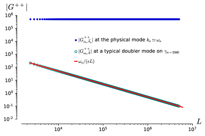
Figure 2: Log-log plots of $|G^{++}_{\omega_{o},\vec{k}_{o}}|$ at the physical mode $k_{o}\simeq\omega_{o}$ (blue dots), and $|G^{++}_{\omega_{o},\vec{k}}|$ at a typical doubler mode on $\gamma_{n}$ with $n=2360$ (green circles). The parameters are $\omega_{o}=50,a_{1}=2^{-50}$ $\epsilon=10^{-4}$. The red line draws $\omega_{o}/(\epsilon L)$ as a function of $L$

In absence of doubling mode, $G_{\omega_{o},\vec{k}}$ is peaked at the physical mode $\vec{k}=\vec{k}_{o}$. In any neighborhood of $\vec{k}_{o}$ and with sufficiently large $L$, $G_{\omega_{o},\vec{k}}$ approximates the continuum fermion propagator arbitrarily well, due to the well-known result $\lim_{L\to\infty}\frac{1}{L}\sum_{n=1}^{L}f_{n}=\lim_{n\to\infty}f_{n}$ for any sequence $\{f_{n}\}$.

We can generalize (2) and consider

$$G_{\omega,\vec{k}}^{(w)}=\sum_{n=1}^{L}|w_{n}|^{2}\chi_{n,\vec{k}}G_{\omega,\vec{k}}(\gamma_{n},a_{n}),$$ (3)

with the generic weight $|w_{n}|^{2}$ satisfying $\sum_{n=1}^{L}|w_{n}|^{2}=1$. $G_{\omega,\vec{k}}^{(w)}$ reduces to $G_{\omega,\vec{k}}$ when the constant weight $|w_{n}|^{2}=1/L$ is chosen. The mechanism of suppressing the doubler modes does not rely on the specific choice of $w_{n}$. Thus our result also applies to $G_{\omega,\vec{k}}^{(w)}$ with generic $w_{n}$.

LQG coupled to chiral fermion.— In the following, we show that the propagator (2) can be derived from LQG with fermion coupling. The 4d spacetime topology is assumed to be $\mathbb{R}\times\Sigma$. A graph $\gamma$ in the spatial slice $\Sigma$ consists of oriented edges $e$ and vertices $v$ as sources and targets of the edges. The LQG Hilbert space $\mathcal{H}$ is given by the direct sum over all graphs $\mathcal{H}=\oplus_{\gamma}\mathcal{H}_{\gamma}/\mathcal{G}$, where $\mathcal{H}_{\gamma}$ is given by $\mathcal{H}_{\gamma}=\mathcal{H}_{\gamma}^{G}\otimes\mathcal{H}_{\gamma}^{F}$, where $\mathcal{H}_{\gamma}^{G}$ is spanned by spin-networks on $\gamma$ with nonzero spins, and $\mathcal{H}_{\gamma}^{F}=\otimes_{v}\mathcal{H}_{v}^{F}$ ($\mathcal{H}_{v}^{F}\simeq\mathbb{C}^{4}$) is the Hilbert space of fermions. $\oplus_{\gamma}\mathcal{H}_{\gamma}$ carries the representation of the holonomy-flux algebra Lewandowski et al. (2006); Ashtekar and Lewandowski (1994) $[\hat{h}_{e},\hat{h}_{e^{\prime}}]=0$, $[\hat{h}_{e},\hat{p}^{a}_{e^{\prime}}]=\beta\ell_{P}^{2}\delta_{e,e^{\prime}}(\bm{\sigma}^{a}/2)\hat{h}_{e}$, $[\hat{p}^{a}_{e},\hat{p}^{b}_{e^{\prime}}]=i\beta\ell_{P}^{2}\delta_{e,e^{\prime}}\varepsilon^{abc}\hat{p}^{c}_{e}$ ($\ell_{P}^{2}=8\pi G\hbar$ and $\beta$ is the Barbero-Immirzi parameter) and the Weyl fermion oscillators $[\hat{\zeta}_{v},\hat{\zeta}_{v^{\prime}}^{\dagger}]_{+}=\delta_{v,v^{\prime}}\mathbf{1}_{2\times 2}$. $\mathcal{G}$ are SU(2) gauge transformations, and $\mathcal{H}$ only contains SU(2) gauge-invariant states. We assume the spatial slice $\Sigma\simeq\mathbb{T}^{3}$ and the periodic boundary condition.

There is a physical Hamiltonian acting on $\mathcal{H}$ Thiemann (2020); Giesel and Thiemann (2015, 2010)

$$\hat{\bf H}=\oplus_{\gamma}\hat{\bf H}_{\gamma},\quad\hat{\bf H}_{\gamma}=\hat{\bf P}_{\gamma}(\hat{H}^{G}_{\gamma}+\hat{H}^{F}_{\gamma})\hat{\bf P}_{\gamma},$$ (4)

where each $\hat{\bf P}_{\gamma}$ is the projection onto $\mathcal{H}_{\gamma}$. $\hat{H}^{G}_{\gamma}$ is identical to the graph-preserving LQG Hamiltonian constraint operator with unit lapse Giesel and Thiemann (2007a, b). $\hat{H}^{F}_{\gamma}$ is the graph-preserving fermion Hamiltonian Lewandowski and Zhang (2021); Thiemann (1998a); Sahlmann and Thiemann (2006); Giesel and Thiemann (2007a). $\hat{H}^{F}_{\gamma}$ is quadratic in $\hat{\zeta}_{v}$: $\hat{H}^{F}_{\gamma}/\hbar=\sum_{\left\langle v,v^{\prime}\right\rangle}\hat{\zeta}_{v}^{\dagger}M_{v,v^{\prime}}(\hat{h},\hat{p})\hat{\zeta}_{v^{\prime}}$ where $M_{v,v^{\prime}}$ is a $2\times 2$ matrix with entries involving only quantum-geometry operators. The detailed expression of $\hat{H}^{G}_{\gamma}+\hat{H}^{F}_{\gamma}$ is reviewed in Appendix A. The theory quantizes Einstein gravity coupling to the Weyl fermion and Gaussian dust in the reduced phase space formulation (relational framework) Kuchar and Torre (1991); Giesel and Thiemann (2015); Han and Liu (2020a); Dittrich (2006); Thiemann (2006); Rovelli (2002, 1991). Semiclassically $h_{e},p_{e}^{a}$ are Dirac observables being the holonomy and flux of the Ashtekar-Barbero variables in the reference frame defined by the Gaussian dust. As a promising aspect, the theory is free of the complications from the quantum Hamiltonian and diffeomorphism constraints, because it quantizes the reduced phase space, where both constraints are resolved at the classical level. All quantities in the theory are Dirac observables from the start.

Initial state.— Based on the above framework of fermion coupling in LQG, the fermion propagator are going to be constructed, and shown to recovers (3) in the semiclassical approximation. As an important ingredient in the fermion propagator, $|\Omega\rangle\in\mathcal{H}$ coupling quantum geometry and fermions needs to be constructed as the LQG analog of the fermion ground state on the semiclassical flat spacetime. Here we define $|\Omega\rangle$ to be an entangled state being the superposition of $|\Omega^{\prime}_{\gamma}\rangle\equiv\hat{\mathbf{P}}_{\gamma}|\psi_{\gamma}\rangle\otimes|\omega_{\gamma}\rangle\in\mathcal{H}_{\gamma}^{G}\otimes\mathcal{H}_{\gamma}^{F}$ over many different graphs $\gamma$, modulo SU(2) gauge transformations. On each $\gamma$, the quantum geometry state $|\psi_{\gamma}\rangle$ is Thiemann’s coherent state peaked at the flat spacetime geometry Thiemann and Winkler (2001a, b). $|\psi_{\gamma}\rangle$ endows $\gamma$ with the semiclassical flat geometry and vanishing extrinsic curvature. $|\omega_{\gamma}\rangle$ is the normalized fermion ground state on the semiclassical flat spacetime, and associates to the lowest energy level of the effective fermion Hamiltonian $\hat{H}_{\gamma}^{F}(\psi_{\gamma})/\hbar=\|\psi_{\gamma}\|^{-2}\sum_{\left\langle v,v^{\prime}\right\rangle}\hat{\zeta}_{v}^{\dagger}\langle\psi_{\gamma}|M_{v,v^{\prime}}(\hat{h},\hat{p})|\psi_{\gamma}\rangle\hat{\zeta}_{v^{\prime}}$. $\hat{H}_{\gamma}^{F}(\psi_{\gamma})$ equals the usual fermion Hamiltonian on the flat lattice plus $O(\ell_{P}^{2})$ corrections (see Appendix B for more details, see also Sahlmann and Thiemann (2006) for the early study of the similar idea).

Any smooth geometry admits many different discretizations based on different graphs. We propose that the semiclassical state of the smooth geometry should be a superposition of states on different graphs, where each state is semiclassical on one graph and relate to the discretization of the smooth geometry on the graph. Here, we consider the smooth geometry to be flat and choose cubic graphs for the satisfactory semiclassical properties at the discrete level Giesel and Thiemann (2007b); Flori and Thiemann (2008). We consider a set of cubic graphs $\{\gamma_{n}\}_{n=1}^{L}$, where $\gamma_{n}$ is a refinement of $\gamma_{1}$ by subdividing every cube into $n^{3}$ cubes. $N_{n}=nN_{1}$ is the number of vertices on $\gamma_{n}$ in every direction. $N_{1}$ is assumed to be even. We define $|\Omega^{\prime}\rangle=\sum_{n=1}^{L}w_{n}|\Omega^{\prime}_{\gamma_{n}}\rangle$, where $|\Omega^{\prime}_{\gamma_{n}}\rangle=\hat{\mathbf{P}}_{\gamma_{n}}|\psi_{\gamma_{n}}\rangle\otimes|\omega_{\gamma_{n}}\rangle$, and the gauge invariant projection

$$|\Omega\rangle=\sum_{n=1}^{L}w_{n}|\Omega_{\gamma_{n}}\rangle,\ \ |\Omega_{\gamma_{n}}\rangle=\hat{\bf P}_{\mathcal{G}}\left(\hat{\mathbf{P}}_{\gamma_{n}}|\psi_{\gamma_{n}}\rangle\otimes|\omega_{\gamma_{n}}\rangle\right).$$

where $\hat{\bf P}_{\mathcal{G}}$ is the (group-averaging) projection onto $\mathcal{H}$. $|\Omega_{\gamma_{n}}\rangle$ are mutually orthogonal and $\|\Omega_{\gamma_{n}}\|=1$. $L$ is finite and large. The weight $w_{n}$ satisfies $\sum_{n=1}^{L}|w_{n}|^{2}=1$ so that $\|\Omega\|=1$. The discrete geometries on $\{\gamma_{n}\}_{n=1}^{L}$ given by $\{|\psi_{\gamma_{n}}\rangle\}_{n=1}^{L}$ are discretizations of the smooth flat geometry, and give the lattice spacings $\{a_{n}\}_{n=1}^{L}$ satisfying $a_{n}=a_{1}/n$. Indeed, the discrete geometry on $\gamma_{n}$ are implied by the expectation values $\langle\psi_{\gamma_{n}}|\hat{h}_{e}|\psi_{\gamma_{n}}\rangle=\mathbf{1}_{2\times 2}+O(\ell_{P}^{2})$ and $\langle\psi_{\gamma_{n}}|\hat{p}^{a}_{e(I)}|\psi_{\gamma_{n}}\rangle=a^{2}_{n}\delta^{a}_{I}+O(\ell_{P}^{2})$, where $e(I)$ is the edge along the $I$-direction. The total spatial volume $V_{\rm tot}=a_{n}N_{n}$ is $n$-independent.

Fermion propagator.— We need the local field operator $\hat{\Psi}(v)$ in order to construct the fermion propagator. However, classically the fermion field $\Psi$ and $\zeta$ are not the same but related by $\zeta=\sqrt[4]{\det(q)}\Psi$, where $\sqrt{\det(q)}$ is the spatial volume density Thiemann (1998b, a). Motivated by the classical relation, we define the fermion field operator by $\hat{\Psi}(v)=\hat{\zeta}_{v}\hat{V}_{v}^{-\frac{1}{2}}$, where $\hat{V}_{v}^{-\frac{1}{2}}$ is the square-root inverse volume (see Appendix A or Giesel and Thiemann (2006); Yang and Ma (2016)). We define the Heisenberg operator $\hat{\Psi}(\tau,v):=e^{\frac{i}{\hbar}\hat{\bf H}(\tau-T_{i})}\hat{\Psi}(v)e^{-\frac{i}{\hbar}\hat{\bf H}(\tau-T_{i})}$ and similarly for $\hat{\Psi}^{\dagger}(\tau,v)$, where $T_{i}$ is the initial time. We prepare the initial state $|\Omega\rangle$ at $T_{i}$ and define the fermion propagator by

$$\mathscr{G}^{AB}(\tau_{1},\tau_{2};v_{1},v_{2})=\langle\Omega^{\prime}|\mathcal{T}[\hat{\Psi}^{A}(\tau_{1},v_{1})\hat{\Psi}^{B}{}^{\dagger}(\tau_{2},v_{2})]|\Omega\rangle,$$

where $\mathcal{T}$ is the time-ordering. Here $v_{1},v_{2}$ are vertices in $\gamma_{1}$, and thus they belong to all the refinements $\gamma_{n}$. $\mathscr{G}^{AB}$ is not SU(2) gauge invariant, as the usual situation in gauge theories. An example of the gauge invariant observable is $\mathscr{G}_{h}(\tau_{1},\tau_{2};v_{1},v_{2})=\langle\Omega|(\hat{h}_{c})_{BA}\mathcal{T}[\hat{\Psi}^{A}(\tau_{1},v_{1})\hat{\Psi}^{B}{}^{\dagger}(\tau_{2},v_{2})]|\Omega\rangle$, where $\hat{h}_{c}$ is the holonomy operator along a path $c\subset\gamma_{1}$ connecting $v_{1},v_{2}$ . In the following, we proceed to compute $\mathscr{G}^{AB}$, then we show $\mathscr{G}_{h}\simeq\mathscr{G}^{AB}\delta_{AB}$ up to $O(\ell_{P}^{2})$.

Since $\hat{\bf H}$ is a direct sum and $|\Omega_{\gamma_{n}}\rangle$ are mutually orthonormal, $\mathscr{G}^{AB}$ is a sum of the fermion propagators on graphs $\{\gamma_{n}\}$

$$\mathscr{G}^{AB}(\tau_{1},\tau_{2};v_{1},v_{2}) = \sum_{n=1}^{L}|w_{n}|^{2}\mathscr{G}_{n}^{AB}(\tau_{1},\tau_{2};v_{1},v_{2})$$ (5)

$$\mathscr{G}_{n}^{AB}(\tau_{1},\tau_{2};v_{1},v_{2}) = \langle\Omega^{\prime}_{\gamma_{n}}|\mathcal{T}[\hat{\Psi}^{A}(\tau_{1},v_{1})\hat{\Psi}^{B}{}^{\dagger}(\tau_{2},v_{2})]|\Omega_{\gamma_{n}}\rangle$$

We compute $\mathscr{G}_{n}^{AB}$ with the time-order $\tau_{1}>\tau_{2}$, while the computation for $\tau_{1}<\tau_{2}$ is similar. We apply the coherent-state path integral method by discretizing the time-evolution operator $e^{-\frac{i}{\hbar}\hat{\bf H}_{\gamma}(\tau-T_{i})}\simeq[1{-\frac{i}{\hbar}\hat{\bf H}_{\gamma}\delta\tau}]^{j_{\tau}}$ with $j_{\tau}\delta\tau={\tau-T_{i}}$ and large $j_{\tau}$, and inserting at each step the over-completeness relation of the coherent state $\int\mathrm{d}Z_{j}(\gamma_{n})|Z_{j}(\gamma_{n})\rangle\langle{Z_{j}(\gamma_{n})}|=1$ ($j=0,\cdots,j_{\tau}$) with $|Z(\gamma_{n})\rangle=|\psi_{(h,p)(\gamma_{n})}\rangle\otimes|\phi_{\zeta({\gamma_{n}})}\rangle$, where $|\psi_{(h,p)(\gamma_{n})}\rangle$ is Thiemann’s coherent state of quantum geometry, and $|\phi_{\zeta({\gamma_{n}})}\rangle$ satisfying $\hat{\zeta}_{v}|\phi_{\zeta({\gamma_{n}})}\rangle=\zeta_{v}|\phi_{\zeta({\gamma_{n}})}\rangle$ is the standard coherent state of the fermion oscillators. $Z(\gamma_{n})$ is a short-hand notation of the data $\{h_{e},p_{e}^{a},\zeta_{v}\}_{e,v}$ where the coherent state is peaked. $\mathrm{d}Z(\gamma_{n})=\mathrm{d}g(\gamma_{n})\prod_{v,A}\mathrm{d}\zeta^{A}_{v}{}^{*}\mathrm{d}\zeta^{A}_{v}$ and $\mathrm{d}g(\gamma_{n})$ denotes the measure of $\{h_{e},p_{e}^{a}\}_{e}$ Thiemann and Winkler (2001a). Following the standard derivation, we obtain the path integral:

$$\mathscr{G}_{n}^{AB} =\int\prod_{j=0}^{N}\mathrm{d}Z_{j}(\gamma_{n})\,e^{S^{G}_{\gamma_{n}}(h,p)+S_{\gamma_{n}}^{F}(h,p,\zeta,\zeta^{*})}$$

$$(V^{-\frac{1}{2}}_{v_{1}}{\zeta}_{v_{1}}^{A})_{j_{1}}(V^{-\frac{1}{2}}_{v_{2}}{\zeta}^{B*}_{v_{2}})_{j_{2}}\langle\Omega^{\prime}_{\gamma_{n}}|Z_{N}(\gamma_{n})\rangle\langle Z_{0}(\gamma_{n})|\Omega_{\gamma_{n}}\rangle$$

where $j_{1,2}=j_{\tau_{1,2}}=(\tau_{1,2}-T_{i})/\delta\tau$ and $N=2j_{1}$. $\langle\Omega^{\prime}_{\gamma_{n}}|Z_{N}(\gamma_{n})\rangle$ and $\langle Z_{0}(\gamma_{n})|\Omega_{\gamma_{n}}\rangle$ are linear in $\zeta_{v}$ and $\zeta_{v}^{*}$ respectively , and the fermion action $S^{F}_{\gamma_{n}}$ is quadratic in $\zeta_{v}$

$$S_{\gamma_{n}}^{F} = \sum_{j,j^{\prime},v,v^{\prime}}\zeta^{\dagger}_{v,j}\mathscr{H}_{v,j;v^{\prime},j^{\prime}}(h,p)\zeta_{v^{\prime},j^{\prime}}$$

$$\mathscr{H}_{v,j;v^{\prime},j^{\prime}} = \delta_{v^{\prime},v}\delta_{j,j^{\prime}+1}-\delta_{j^{\prime},j}\delta_{v^{\prime},v}$$

$$-i\rho_{j}\delta_{j,j^{\prime}+1}{\delta\tau}\left\langle\psi_{g_{j}(\gamma_{n})}\left|M_{v,v^{\prime}}(\hat{h},\hat{p})\right|\psi_{g_{j^{\prime}}(\gamma_{n})}\right\rangle,$$

where $\rho_{j}=1$ or $-1$ at instances before or after $\tau_{1}$. We perform the Gaussian integral of the fermion and obtain the following expression:

$$\!\!\!\!\mathscr{G}_{n}^{AB}=\int\limits_{\mathcal{G}}\mathrm{d}u\int\prod_{j=0}^{N}\mathrm{d}g_{j}(\gamma_{n})\,e^{S^{G}_{\gamma_{n}}}(V^{-\frac{1}{2}}_{v_{1}})_{j_{1}}(V^{-\frac{1}{2}}_{v_{2}})_{j_{2}}\,\mathcal{I}^{AB}_{n}$$ (7)

where $\mathcal{I}^{AB}_{n}=\mathcal{I}^{AB}_{n}(p,h,u)$, resulting from the fermion Gaussian integral, is independent of $\hbar$. The integral over SU(2) gauge transformations $u$ comes from $\mathbf{P}_{\mathcal{G}}$ in $|\Omega_{\gamma_{n}}\rangle$. The effective action of geometry $S^{G}_{\gamma_{n}}$ scales as $1/\ell_{P}^{2}$ as $\ell_{P}\to 0$ Han and Liu (2020b) (see also Appendix C). So the stationary phase approximation can be employed to study the semiclassical approximation of (7). It is shown in Han and Liu (2020b, a) that the equations of motion (EOMs) $\delta S^{G}_{\gamma_{n}}=0$ reproduce the classical Hamilton’s equation of holonomy and fluxes ${\mathrm{d}h_{e}}/{\mathrm{d}\tau}=\{h_{e},H^{G}\}$, ${\mathrm{d}p^{a}_{e}}/{\mathrm{d}\tau}=\{p^{a}_{e},H^{G}\}$, where $H^{G}$ is the discrete gravity Hamiltonian on $\gamma_{n}$ with unit lapse and vanishing shift. The only solution $(\mathring{h},\mathring{p},\mathring{u})$ satisfying the EOMs and compatible to the initial state $|\Omega_{\gamma_{n}}\rangle$ is $\mathring{u}=\mathbf{1}$ and the flat spacetime geometry, where $\mathring{h}_{e,j}=\mathbf{1}_{2\times 2}$ and $\mathring{p}_{e(I),j}^{a}=a_{n}^{2}\delta^{a}_{I}$, i.e. the lattice geometry is constantly flat with spacing $a_{n}$ at all time. Eq.(7) has the following semiclassical approximation

$$\mathscr{G}_{n}^{AB} = a_{n}^{-3}\mathcal{I}_{n}^{AB}(\mathring{p},\mathring{h},\mathring{u})\int\limits_{\mathcal{G}}\mathrm{d}u\int\prod_{j=0}^{N}\!\mathrm{d}g_{j}(\gamma_{n})\,e^{S^{G}_{\gamma_{n}}}\left[1+O(\ell_{P}^{2})\right]$$ (8)

$$= \,a_{n}^{-3}\mathcal{I}_{n}^{AB}(\mathring{p},\mathring{h},\mathring{u})\left[1+O(\ell_{P}^{2})\right].$$

Here the integral removes all fermions degrees of freedom in $\mathscr{G}_{n}$, so it equals $\langle\tilde{\psi}_{\gamma_{n}}|\tilde{\psi}_{\gamma_{n}}\rangle$, where $|\tilde{\psi}_{\gamma_{n}}\rangle\equiv\mathbf{P}_{\mathcal{G}}\mathbf{P}_{\gamma_{n}}|\psi_{\gamma_{n}}\rangle$. $\langle\tilde{\psi}_{\gamma_{n}}|\tilde{\psi}_{\gamma_{n}}\rangle=1+O(\ell_{P}^{2})$ is implied by $\|\Omega_{\gamma_{n}}\|=1$ and $\|\omega_{\gamma_{n}}\|=1$. More details about the semiclassical analysis of $\mathscr{G}_{n}^{AB}$ can be found in Appendix C.

The gauge invariant observable $\mathscr{G}_{h}$ inserts an $({h}_{c})_{AB}$ in the above path integral. Then the stationary phase approximation is (8) contracted by $(\mathring{h}_{c})_{AB}=\delta_{AB}$.

The geometry is freezed to be flat in (8), and $I_{n}^{AB}$ reduces to the standard fermion propagator on the flat lattice with spacing $a_{n}$:

$$\mathscr{G}_{n} = \frac{1}{V_{\rm tot}}\sum_{\vec{k}\in\text{FBZ}(\gamma_{n})}\int_{\mathbb{R}}\frac{\mathrm{d}\omega}{2\pi i}\,e^{-i\omega(\tau_{1}-\tau_{2})+ia_{n}\vec{k}\cdot\left(\vec{v}_{1}-\vec{v}_{2}\right)}$$ (9)

$$G_{\omega,\vec{k}}(\gamma_{n},a_{n})\left[1+O(\ell_{P}^{2})\right],$$

where the continuous limit of time has been taken. The lattice vertices $\vec{v}_{i}\in\mathbb{Z}^{3}$ and $\vec{v}_{i}=\vec{v}_{i}+N_{n}$ ($i=1,2$). The lattice Fourier mode ${k}^{I}\in 2\pi\mathbb{Z}/(N_{1}a_{1})$ is summed over the FBZ on $\gamma_{n}$ with the spacing $a_{n}$.

Insert (9) in (5), and extend the sum of $\vec{k}$ to FBZ on the finest lattice ($\text{FBZ}(\gamma_{n})\subset\text{FBZ}(\gamma_{L})$ for all $n<L$). Notice that $\vec{x}_{1}-\vec{x}_{2}\equiv a_{n}(\vec{v}_{1}-\vec{v}_{2})$ is $n$-independent. The LQG fermion propagator $\mathscr{G}$ becomes

$$\mathscr{G} = \frac{1}{V_{\rm tot}}\sum_{k^{I}\in\text{FBZ}(\gamma_{L})}\int_{\mathbb{R}}\frac{\mathrm{d}\omega}{2\pi i}\,e^{-i\omega(\tau_{1}-\tau_{2})+i\vec{k}\cdot\left(\vec{x}_{1}-\vec{x}_{2}\right)}\mathscr{G}_{\omega,\vec{k}},$$

$$\mathscr{G}_{\omega,\vec{k}} = \sum_{n=1}^{L}|{w}_{n}|^{2}\chi_{n,\vec{k}}G_{\omega,\vec{k}}(\gamma_{n},a_{n})\left[1+O(\ell_{P}^{2})\right].$$ (10)

Up to $O(\ell_{P}^{2})$ corrections, $\mathscr{G}_{\omega,k}$ recovers (3) in which the fermion doublers are suppressed for large $L$.

Discussion.— Our analysis shows that the quantum geometry as the superposition of states with different lattices results in that the fermion propagator from LQG averages the fermion propagators on the lattices. In the resulting fermion propagator, all doubler modes on the lattices are suppressed by the average, while the physical mode are kept unchanged. Our result indicates that the fermion in LQG is free of the doubling problem. It also suggests that the superposition nature of quantum geometry should be the key to resolve the tension between fermion and the fundamental discreteness in QG.

The fact that the superposition of lattices brings the fermion propagator close to the continuum limit suggests that the continuum limit of the full LQG should also relate to the superposition of lattices. This is similar to the approach of group field theory Finocchiaro and Oriti (2021).

Interestingly, the propagator $\mathscr{G}_{\omega,\vec{k}}$ suggests that the quantum geometry provide a soft UV cut-off to fermions. Let us scale $\vec{k}$ large such that $\vec{k}$ is outside $\mathrm{FBZ}(\gamma_{m})$ for certain $m$, then all terms with $n\leq m$ in (10) vanish because of $\chi_{n,\vec{k}}$. Hence, as we scale $\vec{k}$ large, $|\mathscr{G}^{AB}_{\omega,\vec{k}}|$ is suppressed because less and less terms survive in the sum. This result is consistent with the expectation that QG should regularize the UV behavior of matter fields.

We have set the upper bound $L$ of the sum to be finite, so that the lattice refinement gives maximally $(LN_{1})^{3}$ vertices. $L$ actually correlates to $\ell_{P}$, and $L$ has to be finite as far as $\ell_{P}$ is finite. The technical reason is the following: The $O(\ell_{P}^{2})$ correction in $\mathscr{G}_{n}$ may become non-negligible, when the spacing becomes comparable to the Planck length, i.e. $a_{n}\sim\ell_{P}$ Giesel and Thiemann (2007b); Zhang et al. (2022). Fixing $V_{\rm tot}$, $L$ has to be bounded by $L_{0}=V_{\rm tot}^{1/3}/(N_{1}\ell_{P})$ in order that the semiclassical approximation can be applied to all $\mathscr{G}_{n}$ in the sum. Therefore, the refinement limit $L\to\infty$ can only be taken together with the semiclassical limit $\ell_{P}\to 0$. Further investigation is needed to go beyond the semiclassical approximation when computing $\mathscr{G}_{n}$. Then one may consider $L\to\infty$ without the semiclassical limit.

Our result shares the similarity with the random LFT Christ et al. (1982); Pang and Ren (1986); Perantonis and Wheater (1988); Griffin and Kieu (1993) by the average over lattices. But a key difference is that we sum over lattices with different numbers of vertices relating to the lattice refinement, while the random lattice often fixes the number of vertices. It is interesting to further explore the relation to LFT, in order to see the impact from quantum geometry to high energy particle physics. Our computation should extend to n-point functions and further probe the UV behavior. It is also important to study the chiral anomaly on quantum geometry, which is a research undergoing.

Appendix A A. Hamiltonian opertors

In LQG, to promote the classical Hamiltonian of gravity $H^{G}\equiv E-(1+\beta^{2})L$ to the operator, we need to regularize $H^{G}$ based on a graph $\gamma$, and express $H^{G}$ in terms of the basic variables $h_{e}$ and $p_{e}^{a}$. Consider $\gamma$ to be a cubic lattice, and denote by $e(I)$ the edge along the $I$-direction. The quantization of $H^{G}\equiv E-(1+\beta^{2})L$ gives the graph-preserving operator $\hat{H}^{G}_{\gamma}\equiv\hat{E}_{\gamma}-(1+\beta^{2})\hat{L}_{\gamma}$, where

$$\hat{E}_{\gamma} =\frac{-1}{4i\kappa\beta\ell_{P}^{2}}\sum_{v\in V(\gamma)}\sum_{e(I),e(J),e(K)\text{ at }v}\epsilon^{IJK}\tr(h_{\alpha_{IJ}}h_{e(K)}^{-1}[h_{e(K)},\hat{V}_{v}]).$$ (11)

$$\hat{L}_{\gamma} =-\frac{4\kappa}{i\beta^{7}\ell_{P}^{10}}\sum_{v\in V(\gamma)}\sum_{e(I),e(J),e(K)\text{ at }v}\varepsilon^{IJK}\tr([h_{e(I)},[\hat{V}_{\gamma},\hat{E}_{\gamma}]]h_{e(I)}^{-1}[h_{e(J)},[\hat{V}_{\gamma},\hat{E}_{\gamma}]]h_{e_{J}}^{-1}[h_{e(K)},\hat{V}_{v}]h_{e(K)}^{-1})$$

$\alpha_{IJ}$ is a minimal loop in $\gamma$ containing edges $e(I)$ and $e(J)$. $\hat{V}_{v}$ is the volume operator associated to the vertex $v$, and $\hat{V}_{\gamma}=\sum_{v\in V(\gamma)}\hat{V}_{v}$ is the total volume operator.

The fermion Hamiltonian operator is given by $\hat{H}_{\gamma}^{F}=\sum_{\langle v,v^{\prime}\rangle}\hat{\zeta}_{v}^{\dagger}M_{v,v^{\prime}}(\hat{h},\hat{p})\hat{\zeta}_{v^{\prime}}$, where $M_{v,v^{\prime}}(\hat{h},\hat{p})$ reads

$$M_{v,v^{\prime}}(\hat{h},\hat{p})=\delta_{v,v^{\prime}}\hat{V}_{v}^{-\frac{1}{2}}\left(-\frac{(1+3\beta^{2})}{4\beta}\sum_{e\text{ at }v}\hat{p}_{e}^{a}{\bm{\sigma}}_{a}-\frac{\kappa}{i\ell_{P}^{2}\beta}\left[\hat{E}_{\gamma},\hat{V}_{v}\right]\mathbf{1}_{2\times 2}\right)\hat{V}_{v}^{-\frac{1}{2}}$$ (12)

$$-\frac{\beta-i}{4}\left(\sum_{e\text{ at }v}\delta_{v^{\prime},t_{e}}\hat{V}_{v}^{-\frac{1}{2}}{\bm{\sigma}}_{a}\hat{h}_{e}\hat{p}_{e}^{a}\hat{V}_{v}^{-\frac{1}{2}}\right)-\frac{\beta+i}{4}\left(\sum_{e^{\prime}\text{ at }v^{\prime}}\delta_{v,t_{e^{\prime}}}\hat{V}_{v}^{-\frac{1}{2}}\hat{p}_{e^{\prime}}^{a}h_{e^{\prime}}^{-1}{\bm{\sigma}}_{a}\hat{V}_{v}^{-\frac{1}{2}}\right)$$

where $t_{e}$ denotes the target of the edge $e$. Here $\hat{V}_{v}^{-\frac{1}{2}}$, densely defined on $\mathcal{H}$, is not the inverse of $\sqrt{\hat{V}_{v}}$. Indeed, $\sqrt{\hat{V}_{v}}$ takes $0$ as its eigenvalue, so its inverse is not densely defined. $\hat{V}_{v}^{-\frac{1}{2}}$ is obtained by regularizing $\det(e)/\det(q)$ in a neighorhood at $v$ ($\det(e)$ is the determinant of cotriad) Giesel and Thiemann (2006); Yang and Ma (2016). The expression of $\hat{V}_{v}^{-\frac{1}{2}}$ reads

$$\hat{V}_{v}^{-\frac{1}{2}}=-\frac{16}{3}\left(\frac{1}{i\ell_{P}^{2}\beta}\right)^{3}\sum_{e(I),e(J),e(K)\text{ at }v}\epsilon^{IJK}\tr\left([\hat{h}_{e(I)},\hat{V}_{v}^{1/2}]\hat{h}_{e(I)}^{-1}[\hat{h}_{e(J)},\hat{V}_{v}^{1/2}]\hat{h}_{e(J)}^{-1}[\hat{h}_{e(K)},\hat{V}_{v}^{1/2}]h_{e(K)}^{-1}\right).$$ (13)

Semiclassically $\hat{V}_{v}^{-\frac{1}{2}}$ is not always positive, and the sign relates to the orientation $\mathrm{sgn}(\det(e))$. However, the sign is canceled in the classical limit of $M_{v,v^{\prime}}$, since every term contains a pair of $\hat{V}_{v}^{-\frac{1}{2}}$.

Appendix B B. Initial state

Given the cubic graph $\gamma_{n}$, Thiemann’s coherent state $|\psi_{g(\gamma_{n})}\rangle$ is peaked at the phase space point $g(\gamma_{n})\equiv\{h_{e},p_{e}^{a}\}_{e\subset\gamma_{n}}$ Thiemann and Winkler (2001a, b). $h_{e}$ is the SU(2) holonomy of Ashtekar-Barbero connection $\Gamma^{a}_{I}+\beta K^{a}_{I}$ ($\Gamma$ is the spin connection and $K$ is the extrinsic curvature), and $p^{a}_{e}$ smears the densitized triad $\sqrt{\det(q)}\bm{e}^{I}_{a}$ on the 2-face dual to $e$. The expectation values $\langle\psi_{g(\gamma_{n})}|\hat{h}_{e}|\psi_{g(\gamma_{n})}\rangle=h_{e}+O(\ell_{P}^{2})$ and $\langle\psi_{g(\gamma_{n})}|\hat{p}^{a}_{e}|\psi_{g(\gamma_{n})}\rangle=p_{e}^{a}+O(\ell_{P}^{2})$ endow $\gamma_{n}$ with semiclassical internal and external geometries. $|\Omega\rangle\in\mathcal{H}$ relates to $|\psi_{\gamma_{n}}\rangle\equiv|\psi_{g_{\rm flat}(\gamma_{n})}\rangle$ (up to normalization) peeked at the flat geometry $g_{\rm flat}(\gamma_{n})=\{h_{e(I)}=\mathbf{1}_{2\times 2},\,p_{e(I)}^{a}=p_{1}\delta^{a}_{I}\}_{e(I)}$ where $e(I)$ denotes the edge along $I$-direction ($I=1,2,3$). $|\psi_{\gamma_{n}}\rangle$ endow $\gamma_{n}$ with the vanishing extrinsic curvature and the flat lattice geometry with constant lattice spacing $a_{n}=\sqrt{p_{n}}$. The effective fermion Hamiltonian $\hat{H}_{\gamma_{n}}^{F}(\psi_{\gamma_{n}})$ equals the standard fermion Hamiltonian $\hat{\bm{H}}_{\gamma_{n}}^{F}$ on the flat lattice plus $O(\ell_{P}^{2})$ corrections, because $\langle\psi_{\gamma_{n}}|M_{v,v^{\prime}}(\hat{h},\hat{p})|\psi_{\gamma_{n}}\rangle\|\psi_{\gamma_{n}}\|^{-2}$ equals to $M_{v,v^{\prime}}({h},{p})$ evaluated at ${h}_{e}=\mathbf{1}_{2\times 2},\ {p}_{e(I)}^{a}=p_{1}\delta^{a}_{I}$ up to $O(\ell_{P}^{2})$ Giesel and Thiemann (2007b). Namely,

$$\hat{H}_{\gamma_{n}}^{F}(\psi_{\gamma_{n}})=\hat{\bm{H}}_{\gamma_{n}}^{F}\left[1+O(\ell_{P}^{2})\right],\quad\hat{\bm{H}}_{\gamma_{n}}^{F}=\frac{i\hbar}{2a_{n}}\sum_{v\in\gamma_{n}}\sum_{I=1}^{3}\left(\hat{\zeta}_{v}^{\dagger}{\bm{\sigma}}^{I}\hat{\zeta}_{v+\delta_{I}}-\hat{\zeta}_{v+\delta_{I}}^{\dagger}{\bm{\sigma}}^{I}\hat{\zeta}_{v}\right).$$ (14)

It is standard to diagonalize $\hat{\bm{H}}_{\gamma_{n}}^{F}$ by Fourier transformation $\hat{\zeta}_{\vec{k}}=\sqrt{\frac{1}{N_{n}^{3}}}\sum_{v\in\gamma_{n}}\hat{\zeta}_{v}e^{-ia_{n}\vec{k}\cdot\vec{v}}$ ($\vec{v}\in\mathbb{Z}^{3}$ and $\vec{v}=\vec{v}+N_{n}$):

$$\hat{\bm{H}}_{\gamma_{n}}^{F}=\frac{-\hbar}{a_{n}}\sum_{k\in\mathrm{FBZ}(\gamma_{n})}\hat{\zeta}_{k}^{\dagger}\left[\sum_{I=1}^{3}\sin(a_{n}k_{I})\bm{\sigma}^{I}\right]\hat{\zeta}_{k}=\frac{-\hbar}{a_{n}}\sum_{k\in\mathrm{FBZ}(\gamma_{n})}\hat{\zeta}_{k}^{\dagger}\Theta(k)^{\dagger}\left(\begin{array}[]{cc}-\mathfrak{s}({k})&0\\ 0&\mathfrak{s}({k})\end{array}\right)\Theta({k})\hat{\zeta}_{k}$$ (17)

where $\mathfrak{s}({k})=\sqrt{\sum_{I=1}^{3}\sin^{2}(a_{n}k_{I})}$, and $\Theta(k)$ is the unitary matrix diagonalizing $\sum_{I=1}^{3}\sin(a_{n}k_{I})\bm{\sigma}^{I}$. The ground state $|\omega_{\gamma_{n}}\rangle$ associates to the negative zero-point energy $-\mathcal{E}_{0}\equiv-\frac{\hbar}{a_{n}}\sum_{k\in\mathrm{FBZ}(\gamma_{n})}\mathfrak{s}({k})[1+O(\ell_{P}^{2})]$.

The expectation value of physical Hamiltonian $\hat{\bf H}$ at $|\psi_{\gamma_{n}}\rangle\otimes|\omega_{\gamma_{n}}\rangle$ is negative and equals $-\mathcal{E}_{0}$. The existence of zero-point energy is because the fermion Hamiltonian $H_{\gamma}^{F}$ in $\hat{\bf H}$ is not normal ordered. It does not make sense to normal order $H_{\gamma}^{F}$ given that $\hat{\bf H}$ is background independent. Interestingly, we have the semiclassical relation ${\bf H}+E_{\rm dust}=0$ where $E_{\rm dust}$ is the energy of Gaussian dust Giesel and Thiemann (2015); Kuchar and Torre (1991). This relation is one of the starting point of the reduced phase space quantization. Viewing ${\bf H}$ as the expectation value determines $E_{\rm dust}=\mathcal{E}_{0}$. Then $\langle\psi_{\gamma_{n}}|\hat{\bf H}+E_{\rm dust}|\psi_{\gamma_{n}}\rangle=\hat{H}_{\gamma_{n}}^{F}(\psi_{\gamma_{n}})+E_{\rm dust}$ cancels the fermion zero-point energy and gives the normal ordered Hamiltonian on the flat spacetime up to $O(\ell_{P}^{2})$.

Appendix C C. Semiclassical analysis

Figure 3: A $N$-side polygon path starting from $T_{i}$, passing $\tau_{2}$, arriving at $\tau_{1}$ and returning $T_{i}$. $|Z_{0}(\gamma_{n})\rangle$ and $|Z_{N}(\gamma_{n})\rangle$ take the inner products with $|\Omega_{\gamma_{n}}\rangle$ and $|\Omega^{\prime}_{\gamma_{n}}\rangle$ in (20) and (Fermions on Quantum Geometry and Resolution of Doubling Problem).

Let us consider the gauge invariant observable $\mathscr{G}_{h}(\tau_{1},\tau_{2},v_{1},v_{2})$. Similar to (5), we have

$$\mathscr{G}_{h}(\tau_{1},\tau_{2};v_{1},v_{2}) = \sum_{n=1}^{L}|w_{n}|^{2}\mathscr{G}_{h,n}(\tau_{1},\tau_{2};v_{1},v_{2}),$$ (18)

$$\mathscr{G}_{h,n}(\tau_{1},\tau_{2};v_{1},v_{2}) = \langle\Omega_{\gamma_{n}}|(\hat{h}_{c})_{BA}\mathcal{T}[\hat{\Psi}^{A}(\tau_{1},v_{1})\hat{\Psi}^{B}{}^{\dagger}(\tau_{2},v_{2})]|\Omega_{\gamma_{n}}\rangle.$$ (19)

We can obtain the path integral formula of $\mathscr{G}_{h,n}(\tau_{1},\tau_{2};v_{1},v_{2})$ on $\gamma_{n}$ as

$$\mathscr{G}_{h,n}(\tau_{1},v_{1},\tau_{2},v_{2}) =\int\limits_{\mathcal{G}}\differential u\int\prod_{j=0}^{N}\mathrm{d}g_{j}(\gamma_{n})e^{S^{G}_{\gamma_{n}}(g,u)}((\hat{h}_{c})_{BA})_{N}(V^{-\frac{1}{2}}_{v_{1}})_{j_{1}}(V^{-\frac{1}{2}}_{v_{2}})_{j_{2}}\mathcal{I}^{AB}_{n}(g,u)$$ (20)

$$\mathcal{I}^{AB}_{n}(g,u) =\int\prod_{j=0}^{N}\differential\zeta_{j}(\gamma_{n})\,e^{S^{F}_{\gamma_{n}}(g,\zeta)}(\zeta_{v_{1}}^{A})_{j_{1}}(\zeta_{v_{2}}^{B*})_{j_{2}}\langle\omega_{\gamma_{n}}|\phi_{\zeta_{N}}\rangle\langle\phi_{\zeta_{0}}|u|\omega_{\gamma_{n}}\rangle$$

where the integral with respect $u=\{u_{v}\}_{v}\in\mathcal{G}$ comes from the projection $\hat{\mathbf{P}}_{\mathcal{G}}$ introduced in defining $|\Omega_{\gamma_{n}}\rangle$. A pair of $\langle\Omega_{\gamma_{n}}$ and $|\Omega_{\gamma_{n}}\rangle$ only give one $u$-integral because the operator is gauge invariant and $\hat{\mathbf{P}}_{\mathcal{G}}^{2}=\hat{\mathbf{P}}_{\mathcal{G}}$.

In the derivation of the path integral, we insert the Heisenberg operator in $\mathscr{G}_{h}$, and have the following expression in terms of the time-evolution operators

$$\mathscr{G}_{h,n}(\tau_{1},v_{1},\tau_{2},v_{2})=\langle\Omega_{\gamma_{n}}|(\hat{h}_{c})_{BA}e^{\frac{i}{\hbar}\hat{\bf H}_{\gamma_{n}}(\tau_{1}-T_{i})}\hat{\Psi}^{A}(v)e^{-\frac{i}{\hbar}\hat{\bf H}_{\gamma_{n}}(\tau_{1}-\tau_{2})}\hat{\Psi}^{B\dagger}(v)e^{-\frac{i}{\hbar}\hat{\bf H}_{\gamma_{n}}(\tau_{2}-T_{i})}|\Omega_{\gamma_{n}}\rangle,$$ (21)

when $\tau_{1}>\tau_{2}$. It leads to that in the path integral (20), the paths $Z_{j}(\gamma_{n})\equiv(g_{j}(\gamma_{n}),\zeta_{j}(\gamma_{n}))$ start from $T_{i}$, pass $\tau_{2}$, arrive at $\tau_{1}$, and finally return to $T_{i}$. As in the standard derivation, we begin with considering the $N$-side polygon paths as shown in Fig. 3 and, then, let $N$ approaches to $\infty$. In (20) and (7), $S_{\gamma_{n}}^{G}$ reads

$$S_{\gamma_{n}}^{G}= \sum_{j=-1}^{N}\sum_{e\subset\gamma_{n}}\frac{2\eta_{j+1,j}(e)^{2}-\eta_{j+1,j+1}(e)^{2}-\eta_{j,j}(e)^{2}}{2\ell_{P}^{2}}-\frac{i}{\hbar}\sum_{\begin{subarray}{c}j=0\end{subarray}}^{N-1}\rho_{j}\delta\tau\left(\frac{\langle\psi_{g_{j+1}(\gamma_{n})}|\hat{\mathbf{P}}_{\gamma_{n}}\hat{H}_{\gamma_{n}}^{G}\hat{\mathbf{P}}_{\gamma_{n}}|\psi_{g_{j}(\gamma_{n})}\rangle}{\langle\psi_{g_{j+1}(\gamma_{n})}|\psi_{g_{j}(\gamma_{n})}\rangle})\right),$$

where $\rho_{j}=1$ or $-1$ at instances before or after $\tau_{1}$. $j=-1$ and $j=N+1$ correspond to the initial and final state. The coherent label $g_{j}(\gamma_{n})=\{g_{e}\}_{e\subset\gamma_{n}}$ relates to $h_{e},p_{e}^{a}$ by $g_{e}=e^{-p_{e}^{a}\bm{\sigma}^{a}/2}h_{e}$. $\eta_{i,j}(e)$ satisfies $\tr(g_{i}^{\dagger}(e)g_{j}(e))=2\cosh(\eta_{i,j}(e))$. At $j=-1$, $g_{-1}(\gamma_{n})=u\cdot g_{\rm flat}(\gamma_{n})$ is the gauge transformation of $g_{\rm flat}(\gamma_{n})$.

$\mathcal{I}^{AB}_{n}$ is independent of $\hbar$. The integral of $\differential u$ and $\differential g_{j}(\gamma_{n})$ is studied with the stationary phase approximation to obtain a semiclassical expansion in $\ell_{P}^{2}$. With the chosen initial and final states, the solution of equations of motion gives $u=\mathring{u}=\mathbf{1}$ for all vertices $v$ and $g=\mathring{g}(\gamma_{n})=(\mathring{p},\mathring{h})$ corresponding to the flat spacetime: $\mathring{h}_{e,j}=\mathbf{1}_{2\times 2}$ and $\mathring{p}_{e(I),j}^{a}=a_{n}^{2}\delta^{a}_{I}$. Thus as far as the leading order in the semiclassical expansion is concerned, we can just freeze $u$ in $\mathcal{I}_{n}^{AB}$ to $\mathbf{1}$, and freeze $((\hat{h}_{c})_{BA})_{N}(V^{-\frac{1}{2}}_{v_{1}})_{j_{1}}(V^{-\frac{1}{2}}_{v_{2}})_{j_{2}}$ to their corresponding classical value at the flat geometry. Therefore, Eq.(20) can be approximated by $\delta_{BA}\mathscr{G}^{AB}_{n}$ semiclassically, where $\mathscr{G}^{AB}_{n}$ is given by

$$\mathscr{G}^{AB}_{n}=\frac{1}{V_{\rm tot}}\mathcal{I}^{AB}_{n}(\mathring{g},\mathring{u})\int\limits_{\mathcal{G}}\mathrm{d}u\int\prod_{j=0}^{N}\mathrm{d}g_{j}(\gamma_{n})\,e^{S^{G}_{\gamma_{n}}(g,u)}\left[1+O(\ell_{P}^{2})\right]$$

The integral $\int\mathrm{d}u\int\prod_{j=0}^{N}\mathrm{d}g_{j}(\gamma_{n})\,e^{S^{G}_{\gamma_{n}}(g,u)}$ is the transition amplitude between a pair of $|\tilde{\psi}_{\gamma_{n}}\rangle\equiv\hat{\mathbf{P}}_{\mathcal{G}}\hat{\mathbf{P}}_{\gamma_{n}}|\psi_{\gamma_{n}}\rangle$, the quantum-geometry sectors of the initial state, with respect to the pure gravity Hamiltonian $\hat{\mathfrak{h}}_{\gamma_{n}}^{G}\equiv\hat{\mathbf{P}}_{\gamma_{n}}\hat{H}_{\gamma_{n}}^{G}\hat{\mathbf{P}}_{\gamma_{n}}$. Recall that the paths are the ones as in FIG.3. We have

$$\int\limits_{\mathcal{G}}\mathrm{d}u\int\prod_{j=0}^{N}\mathrm{d}g_{j}(\gamma_{n})\,e^{S^{G}_{\gamma_{n}}(g,u)}=\langle\tilde{\psi}_{\gamma_{n}}|e^{\frac{i}{\hbar}\hat{\mathfrak{h}}^{G}_{\gamma_{n}}(\tau_{1}-T_{i})}e^{-\frac{i}{\hbar}\hat{\mathfrak{h}}^{G}_{\gamma_{n}}(\tau_{1}-\tau_{2})}e^{-\frac{i}{\hbar}\hat{\mathfrak{h}}^{G}_{\gamma_{n}}(\tau_{2}-T_{i})}|\tilde{\psi}_{\gamma_{n}}\rangle=\langle\tilde{\psi}_{\gamma_{n}}|\tilde{\psi}_{\gamma_{n}}\rangle=1+O(\ell_{P}^{2}).$$

where in the last step, we use $1=\langle\Omega_{\gamma_{n}}|\Omega_{\gamma_{n}}\rangle=\int_{\mathcal{G}}\mathrm{d}u\langle\psi_{\gamma_{n}}|\mathbf{P}_{\gamma_{n}}u\mathbf{P}_{\gamma_{n}}|\psi_{\gamma_{n}}\rangle\langle\omega_{\gamma}|u|\omega_{\gamma}\rangle=\int\mathrm{d}u\langle\psi_{\gamma_{n}}|\mathbf{P}_{\gamma_{n}}u\mathbf{P}_{\gamma_{n}}|\psi_{\gamma_{n}}\rangle[1+O(\ell_{P}^{2})]$, because $\|\omega_{\gamma_{n}}\|=1$ and $\langle\psi_{\gamma_{n}}|\mathbf{P}_{\gamma_{n}}u\mathbf{P}_{\gamma_{n}}|\psi_{\gamma_{n}}\rangle$ is a Gaussian-like function peaked at $u=\mathbf{1}$. Therefore

$$\mathscr{G}^{AB}_{n}=\frac{1}{V_{\rm tot}}\mathcal{I}^{AB}_{n}(\mathring{g},\mathring{u})[1+O(\ell_{P}^{2})].$$

Substituting the flat-geometry data $\mathring{p}$ and $\mathring{h}$ into $S^{F}_{\gamma_{n}}$, and performing the Fourier transformation to $\zeta_{i,v}$ along spatial directions, we get $S_{\gamma_{n}}^{F}$ in terms of the Fourier coefficients $\zeta_{j,\vec{k}}$ as $S_{N}^{F}=\sum_{j,\vec{k},j^{\prime},\vec{k}^{\prime}}\zeta_{j,\vec{k}}^{\dagger}\mathscr{H}_{j,\vec{k},j^{\prime},\vec{k}^{\prime}}\zeta_{j^{\prime},\vec{k}^{\prime}}$, with $\mathscr{H}_{j,\vec{k},j^{\prime},\vec{k}^{\prime}}=-\delta_{j,j^{\prime}}\mathbf{1}_{2\times 2}+\delta_{j,j^{\prime}+1}\left(\mathbf{1}_{2\times 2}+\frac{i\delta\tau}{a_{n}}\sum_{I=1}^{3}\sin(a_{n}k_{I}){\bm{\sigma}}^{I}\right)$. With these results, $\mathcal{I}^{AB}_{n}(\mathring{g},\mathring{u})$ can be computed by using the standard Fermionic Gaussian integral. The result is obtained by taking the limit $N\to\infty$:

$$\mathcal{I}^{AB}_{n}(\mathring{g},\mathring{u})=\sum_{\vec{k}\in\text{FBZ}(\gamma_{n})}\int_{\mathbb{R}}\frac{\mathrm{d}\omega}{2\pi i}\,e^{-i\omega(\tau_{1}-\tau_{2})+ia_{n}\vec{k}\cdot\left(\vec{v}_{1}-\vec{v}_{2}\right)}\,G_{\omega,\vec{k}}(\gamma_{n},a_{n}).$$ (22)