SOFIA observations of 30 Doradus: II - Magnetic fields and large scale gas kinematics

Abstract

The heart of the Large Magellanic Cloud, 30 Doradus, is a complex region with a clear core-halo structure. Feedback from the stellar cluster R 136 has been shown to be the main source of energy creating multiple pc-scale expanding-shells in the outer region, and carving a nebula core in the proximity of the ionization source. We present the morphology and strength of the magnetic fields (B-fields) of 30 Doradus inferred from the far-infrared polarimetric observations by SOFIA/HAWC+ at 89, 154, and 214$\,\mu$m. The B-field morphology is complex, showing bending structures around R 136. In addition, we use high spectral and angular resolution [CII] observations from SOFIA/GREAT and CO(2-1) from APEX. The kinematic structure of the region correlates with the B-field morphology and shows evidence of multiple expanding shells. Our B-field strength maps, estimated using the Davis-Chandrasekhar-Fermi method and structure-function, show variations across the cloud within a maximum of 600, 450, and 350$\,\mu$G at 89, 154, and 214$\,\mu$m, respectively. We estimated that the majority of the 30 Doradus clouds are sub-critical and sub-Alfvénic. The probability distribution function of the gas density shows that the turbulence is mainly compressively driven, while the plasma beta parameter indicates supersonic turbulence. We show that the B-field is sufficient to hold the cloud structure integrity under feedback from R 136. We suggest that supersonic compressive turbulence enables the local gravitational collapse and triggers a new generation of stars to form. The velocity gradient technique (VGT) using [CII] and CO(2-1) is likely to confirm these results.

1 Introduction

In modern Astrophysics, magnetic fields (B-fields) and turbulence are believed to affect the star-formation process. The B-fields support against gravitational collapse, while turbulence plays a dual role. Turbulence can against cloud global collapse, but can also produce local compression (Mac Low & Klessen 2004) with the compressible and solenoidal motions acting in the opposite directions (Cho & Lazarian 2003). The role of B-fields can be different depending on whether B-fields are dynamically important or subdominant (see a review in Crutcher 2012). For weak B-fields, the cloud is super-critical (the mass-to-flux ratio is greater than unity), and the B-fields are insufficient to prevent gravitational collapse. For strong B-fields, the fields are strong enough to counteract the collapse. In this case, other mechanisms must be invoked for star formation to occur in the sub-critical cloud (the mass-to-flux ratio is lower than unity). There are two candidates for such mechanisms: (1) ambipolar diffusion (e.g., Mestel 1966) can increase the mass faster than the B-field strength, enhancing the gravitational counterpart, and (2) fast turbulent reconnection (Lazarian & Vishniac 1999) removes the magnetic flux, weakening the magnetic support. These two mechanisms are able to increase the mass-to-flux ratio, which can lead clouds to collapse and possibly to co-exist (Lazarian 2014).

The fast turbulent reconnection induces a turbulence cascade perpendicular to the ambient B-fields. As a result, turbulent eddies can freely mix the B-fields parallel to the rotation axes, where the velocity gradients (VGs) are perpendicular to the local direction of B-fields. This is the basis of the velocity gradient technique (VGT; González-Casanova & Lazarian 2017) to study B-fields in diffuse gas (Yuen & Lazarian 2017a; Lazarian & Yuen 2018; Lazarian et al. 2018; Hu et al. 2018, 2019a), in molecular clouds (Hu et al. 2019b; Tang et al. 2019; Hu et al. 2021a, b; Alina et al. 2022), and in the atomic-molecular transition (Skalidis et al. 2021b). Nevertheless, self-gravity is able to break that relationship. The gravitational forces pull the gas in the direction along the B-fields, so the VGs are dominated by the infall acceleration. In this case, the VGs are parallel to the ambient B-fields. The misalignment between VGT and B-fields becomes a proxy for the gravitational collapse (Yuen & Lazarian 2017b;Lazarian & Yuen 2018;Tang et al. 2019; Hu et al. 2021a). Therefore, VGT is a promising tool to probe the B-fields morphology and the local gravitational collapse.

The B-fields, turbulence, and stellar feedback shape the cloud and regulate the star-formation processes. The simulations with uniform B-fields from Henney et al. (2009) and Mackey & Lim (2011) showed that the B-fields have a significant contribution in shaping the cloud. This result depends on the orientation between the initial B-fields and the radiation from the source. Specifically, these authors found that clouds are flatter (broad head) if the B-fields are parallel to the radiation direction, while the cloud becomes a more elongated structure (tail-like structure) if the B-fields are perpendicular to the radiation direction. These features appear to be confirmed from observations, e.g., IC 1396 (Soam et al. 2018a), M16 (Pattle et al. 2018), Ophiuchus-A (Santos et al. 2019). The simulations of the feedback in a turbulent magnetized cloud by Arthur et al. (2011) showed that the B-fields tend to be amplified and slow down the formation of stars.

The morphology of the B-fields is affected by gravity (resulting in a well-known hour-glass shape; Ewertowski & Basu 2013), and regulated by the supersonic gas motion as proposed by Inoue & Fukui (2013). The latter seems to be frequently observed, e.g., deformation of B-field geometry in M16 (Pattle et al. 2018), Orion-A (Tahani et al. 2019), Musca filament (Bonne et al. 2020a, b) and BHR 71 bipolar outflow system (Kandori et al. 2020). Using simulations, Abe et al. (2021) demonstrated that a shock with a velocity of $\sim 7\,\rm km\,s^{-1}$ is able to wrap the B-fields.

Even though B-fields may affect the star formation processes, the direct measurement of B-fields is difficult. Alternatively, the B-fields are inferred using several data analysis methods. One of the methods consists in using dust polarization (see e.g., Lazarian 2007 and Andersson et al. 2015 for reviews). The basic idea of this technique relies on the fact that irregular dust grains tend to align with their shortest axis parallel to the local B-fields due to various physical effects (see e.g., Hoang et al. 2022 for details) so that their thermal emission is polarized with the polarization vector perpendicular to the B-fields (see Tram & Hoang 2022). The measured position angle of thermal dust polarization is then perpendicular to the local B-fields in the plane of the sky. Hence, the polarimetric data allows us to map the B-field geometry by rotating the polarization angles (E-vectors) by $90^{o}$. The polarized thermal dust emission is feasible at long wavelengths, i.e., FIR to submm. The strength of the B-fields on the plane of the sky ($B_{\rm POS}$) can be estimated using the Davis-Chandrasekhar-Fermi (DCF; Davis 1951; Chandrasekhar & Fermi 1953) method. This method is commonly used, although some modifications need to be taken into account as a function of the object to be analyzed (Liu et al. 2022). Another approach (namely Differential Measure Approach or DMA) is recently proposed by Lazarian et al. (2020, 2022), which is suggested to be able to measure the B-field strength locally.

Our target is the star-formation region, 30 Doradus (hereafter 30 Dor) in the Large Magellanic Cloud (LMC). With a distance of $\simeq 50\,$kpc away from Earth (Schaefer 2008), it is close enough to obtain parsec-scale resolutions to study the impact of the feedback and turbulence on the surrounding molecular cloud. 30 Dor hosts a massive star cluster, R 136, which is associated to the HII giant expanding-shells (Kennicutt 1984; Chu & Kennicutt 1994; Brandl 2005; Townsley et al. 2006; Lopez et al. 2011), and a nearby Supernova Remnant (Townsley et al. 2006). Figure 1 shows a composite image of the 30 Dor region with an overlaid of the field-of-view covered in our study. This complex system is embedded by multiple HI giant-shells (Kim et al. 1999). A combination of stellar winds and supernovae (Chu & Kennicutt 1994) or only the cluster-wind (not the stellar wind of individual stars) from R 136 (Melnick et al. 2021) are demonstrated to be the main sources to create these giant HII expanding-structures. The authors also clearly unveiled two structures in 30 Dor. For the nebula’s core (within a distance of $25\,\rm pc$ proximity to R 136), surprisingly, the thermal gas pressure is lower than that of the stellar radiation (see figure 18 in Pellegrini et al. 2011), and the mass is lower than the virial mass (Melnick et al. 2021). Hence, the important questions remaining are: how can this structure survive? and how can stars form? (the locations of protostar candidates are shown in e.g., Lee et al. 2019; Indebetouw et al. 2009). Here, we focus on the closest region to R 136, which is indicated by the white box in Figure 1. For the sake of simplicity, we refer to this region as 30 Dor in this work.

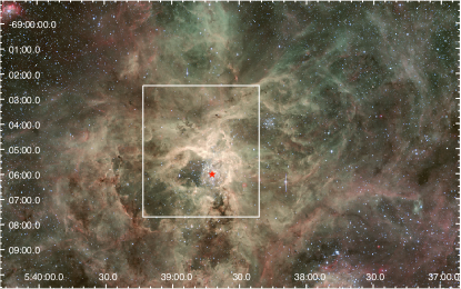
Figure 1: Public composite image of 30 Dor observed by La Silla 2.2 m telescope with $H_{\alpha}$-658.827 nm (red), a combination of V-539.562 nm and [OIII]-502.393 nm (green), and B-451.100 nm (blue). This image shows a complex structure of the region with multiple large expanding shells produced by the hot cluster-wind from R 136 (indicated by a red star), and a slow expanding-shell from the supernova remnant 30DorB (lower right). The white box shows the region covered by SOFIA/HAWC+ that we analyze in this work.

Our goals are to

• map the morphology and strength of the B-fields in 30 Dor using FIR polarimetric observations with SOFIA/HAWC+ as introduced in Tram et al. (2021c) (hereafter Paper I);

• examine the gas kinematic in 30 Dor by making use of [CII] and CO(2-1) data acquired by SOFIA/GREAT and APEX (see Okada et al. 2019);

• make use of the VGT to probe the local gravitational collapse in 30 Dor;

• quantify the effect of B-fields on supporting the cloud integrity; and

• perform an energy budget to quantify the effect of gravity, B-fields, and turbulence on the star-forming processes of 30 Dor.

This paper is structured as follows. We analyze the gas kinematics in Section 2. The analysis of the B-field orientations and strengths are shown in Section 3. Our discussions are presented in Section 4. The conclusions are presented in Section 5.

2 Large scale kinematics in 30 Doradus

To analyze the pc scale kinematics of 30 Dor at the location of the HAWC+ observations, we make use of the spectral lines presented in Okada et al. (2019) that were observed with SOFIA (Young et al., 2012) & the APEX telescope (Güsten et al., 2006). For details on the data reduction, we refer to Okada et al. (2019). The SOFIA observations of the [CII] line have a spatial resolution of 16^′′ and the APEX CO(2-1) observations have a spatial resolution of 30^′′. The region of the HAWC+ map and of the [CII] and ¹²CO(2-1) is presented in Figure 2. Both lines cover a similar area of 30 Dor where the dust polarization is detected.

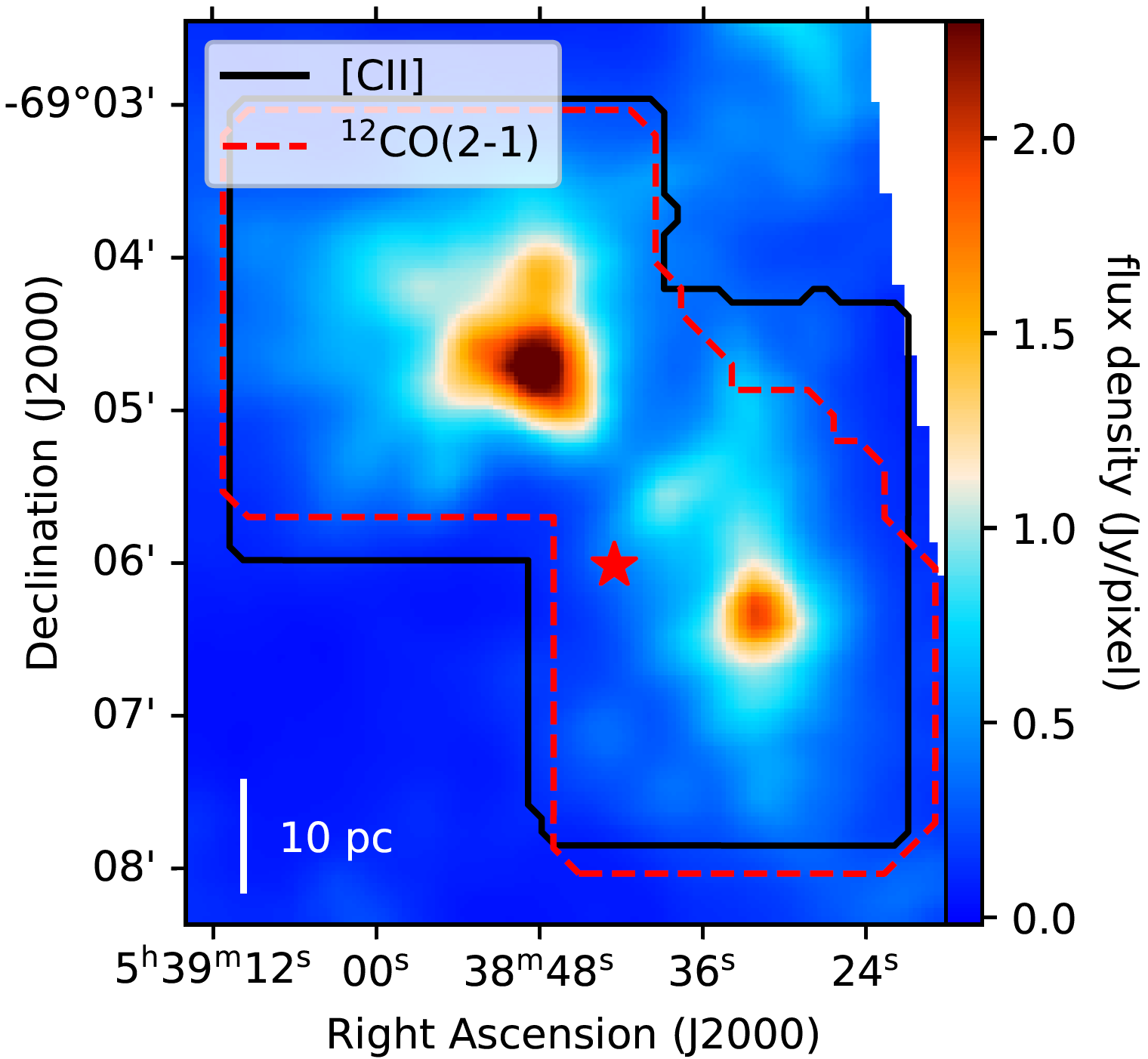
Figure 2: HAWC+ dust continuum flux density map at 214$\,\mu$m. The black full line indicates the region that is covered by the [CII] observations and the red dashed line outlines the region covered by the ¹²CO(2-1) observations (Okada et al. 2019). The red star indicates the location of R136.

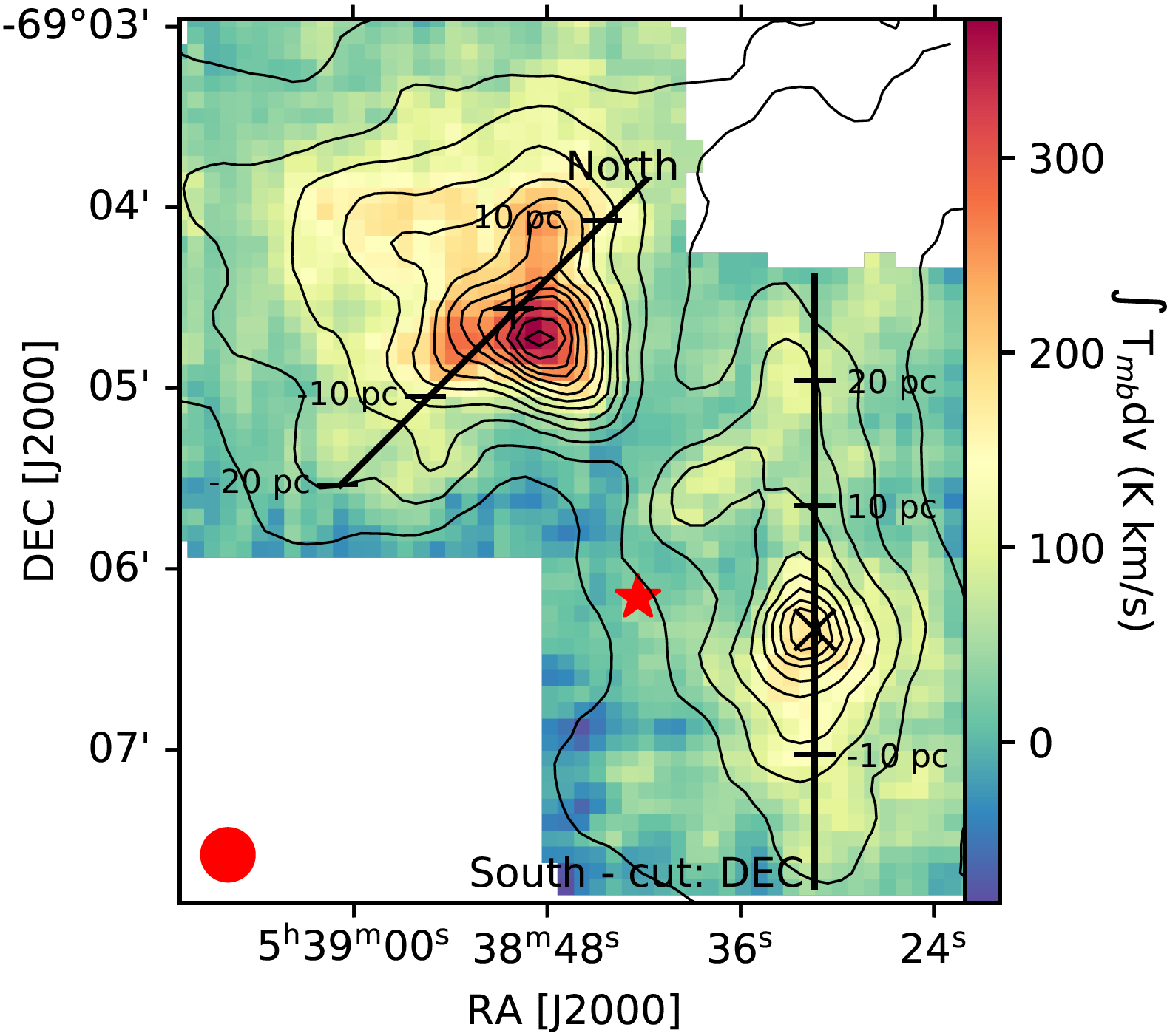
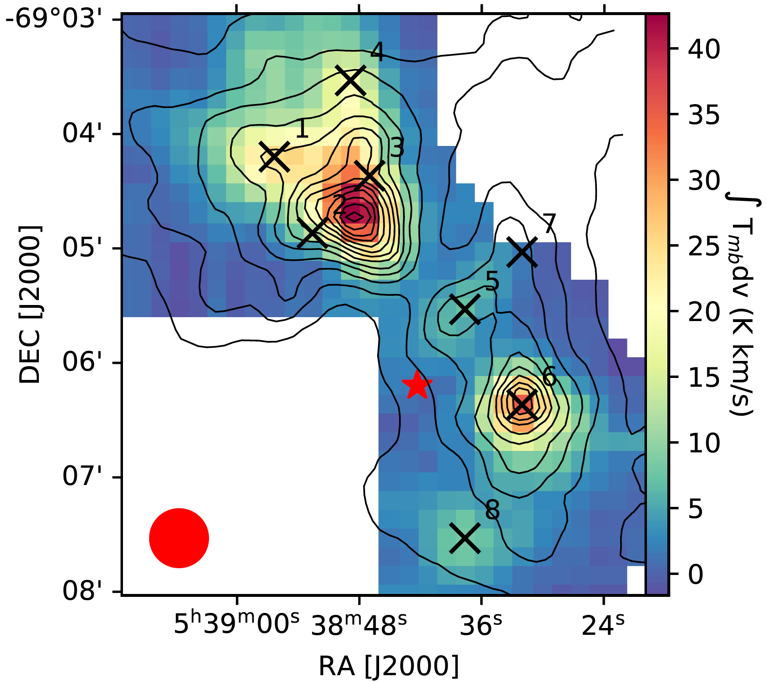
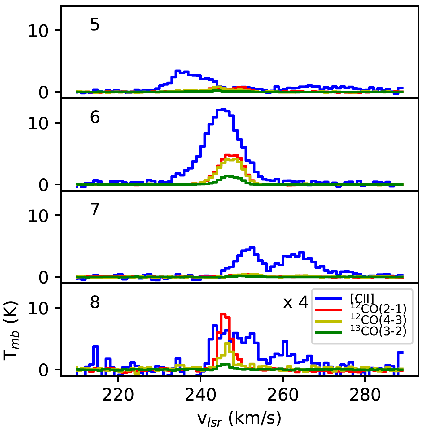
Figure 3: Left: [CII] integrated intensity map of 30 Dor. The black contours show the HAWC+ dust continuum emission at 214$\,\mu$m starting at 0.1 Jy pixel^-1 with increments of 0.1 Jy pixel^-1. The two lines indicate the spatial axes that were used to construct the position-velocity (PV) diagrams presented in Figure 6. The crosses indicate the center, i.e. 0 pc, of the PV diagrams, and the horizontal locations indicate the physical distance along the axis at the location of 30 Dor. The red star indicates the location of R136. Right: The integrated intensity map of ¹²CO(2-1), overlaid with the same HAWC+ contours shown on the left. The crosses indicate the spatial locations of the spectra shown below. Bottom: The extracted [CII], ¹²CO(2-1), ¹²CO(4-3) and ¹³CO(3-2) spectra at the indicated locations over the 30 Dor region, displaying multiple components and several wings in [CII].

2.1 The integrated intensity maps

In Figure 3, the integrated intensity maps of [CII] and ¹²CO(2-1) are compared with the dust continuum maps from HAWC+ at 214$\,\mu$m. This figure shows that the [CII] peak intensities are closely correlated with the dust continuum peak and that it also traces the extended emission. We find that ¹²CO(2-1) is more sensitive to the gas located in the high column density regions, which can be expected for this lower metallicity region. As a result, the [CII] emission will be more sensitive to the kinematics of the ambient gas, whereas CO is more sensitive to the dense clumps in the cloud.

2.2 The velocity structure of 30 Doradus

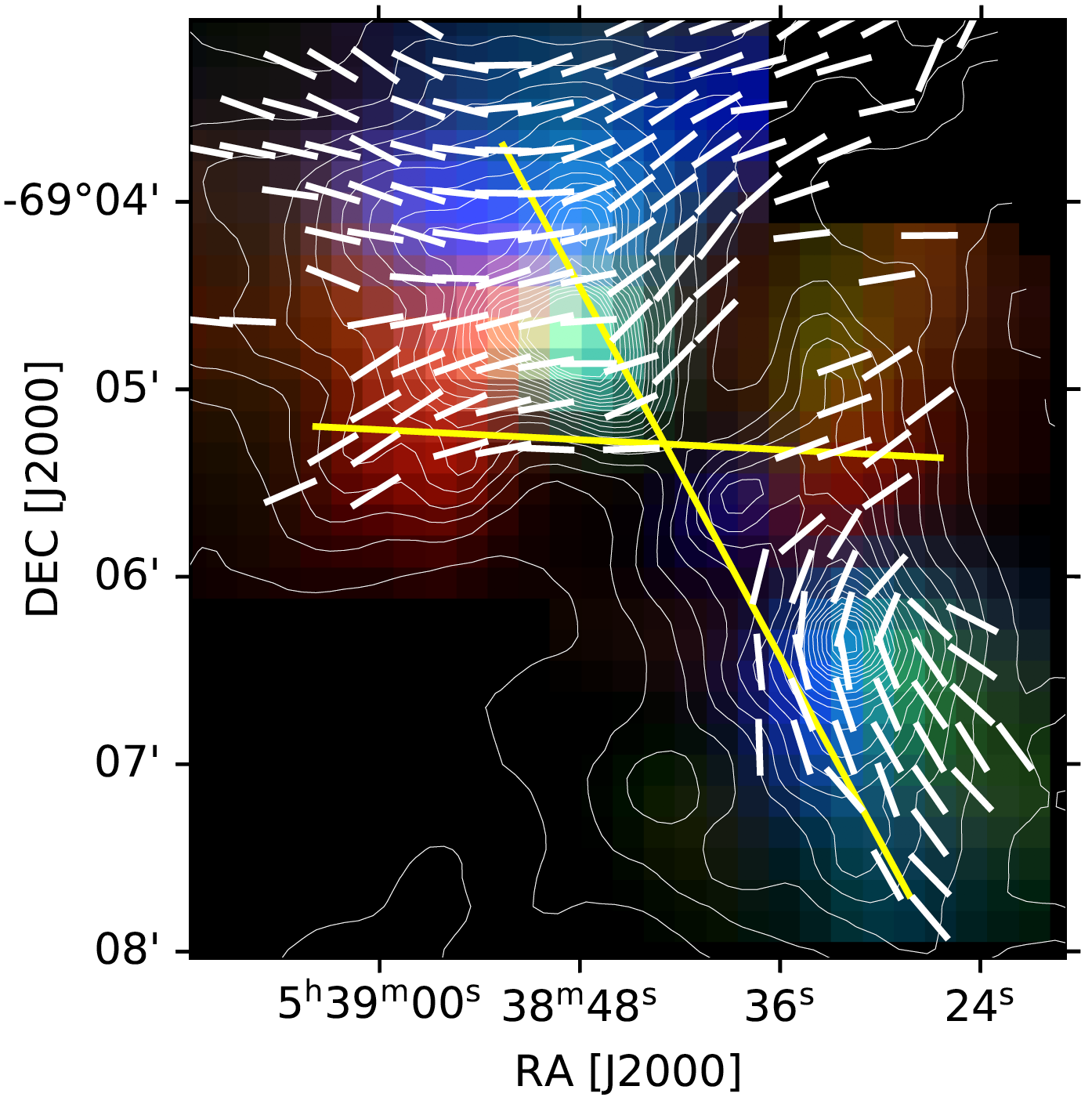
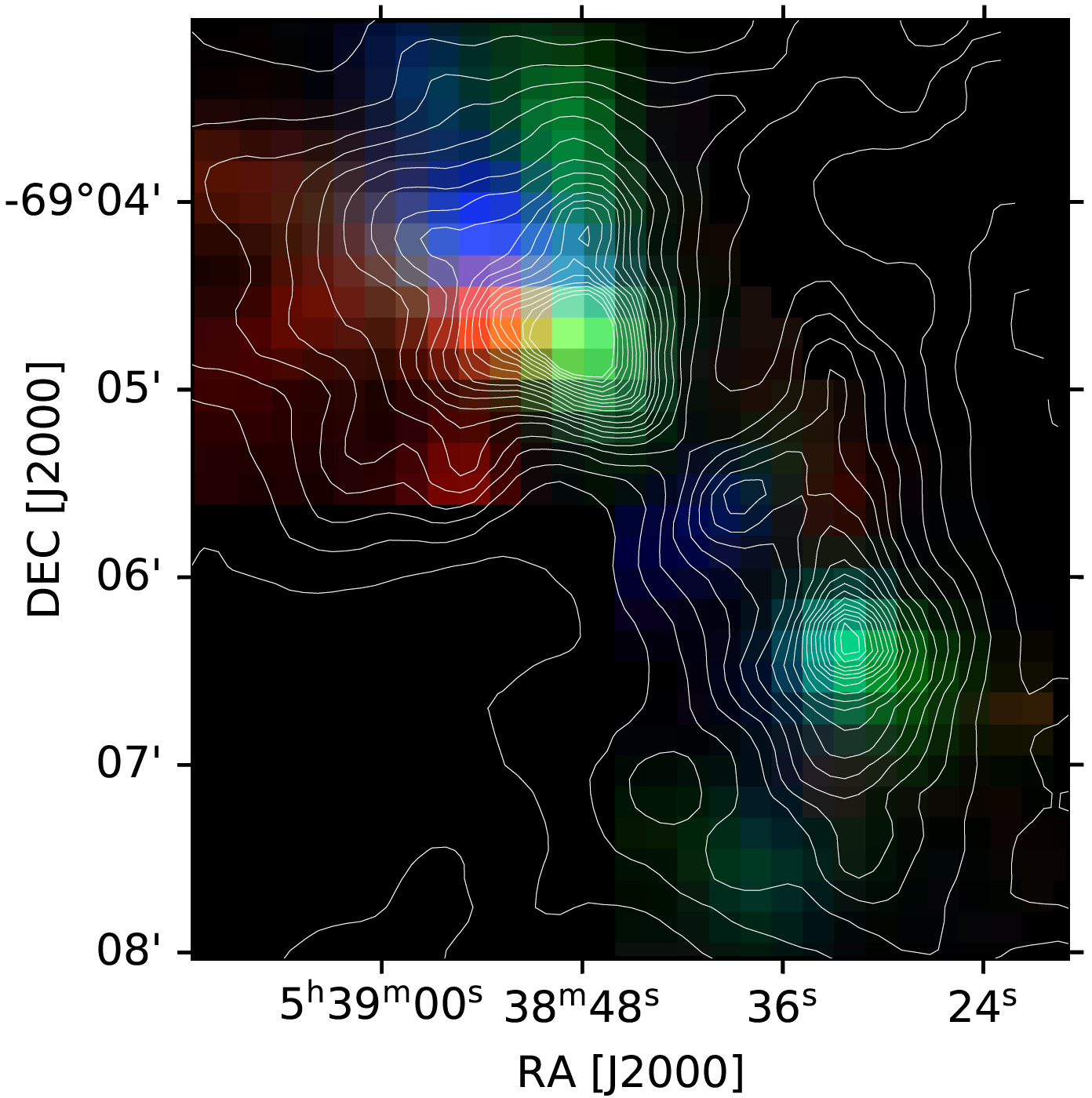
Figure 4: Left: RGB image of 30 Dor for [CII] with blue: 235-245$\,\rm km\,s^{-1}$, green: 245-255$\,\rm km\,s^{-1}$ and red: 255-270$\,\rm km\,s^{-1}$. The contours indicate the HAWC+ 214$\,\mu$m dust continuum emission starting at 0.1 Jy pixel^-1 with increments of 0.1 Jy pixel^-1. The yellow cross is added to guide the eye at the axes of what appears to be dominantly blue- and red-shifted gas. The white segments indicate the magnetic field morphology on the RGB image. Right: The same for ¹²CO(2-1).

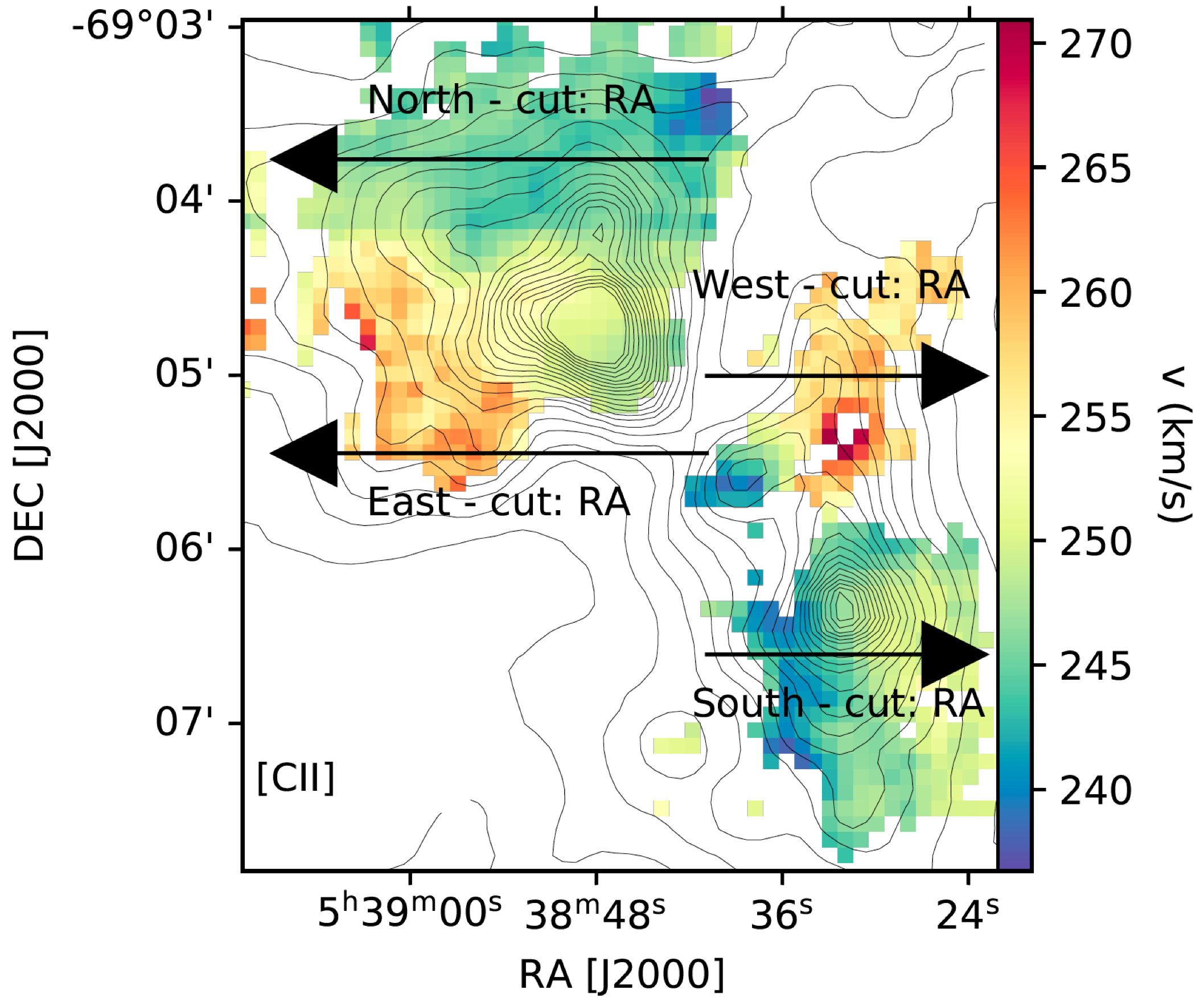
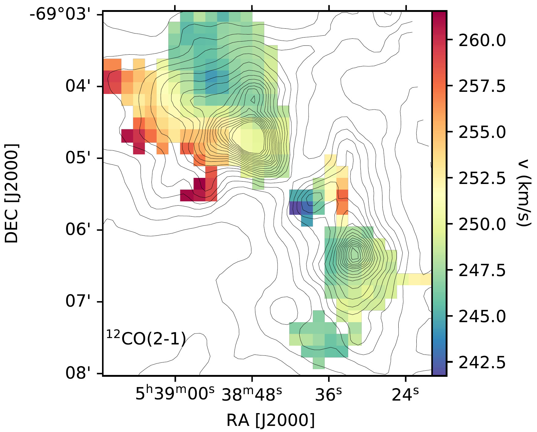
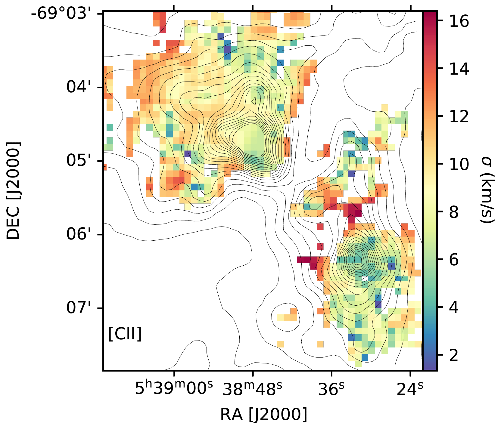
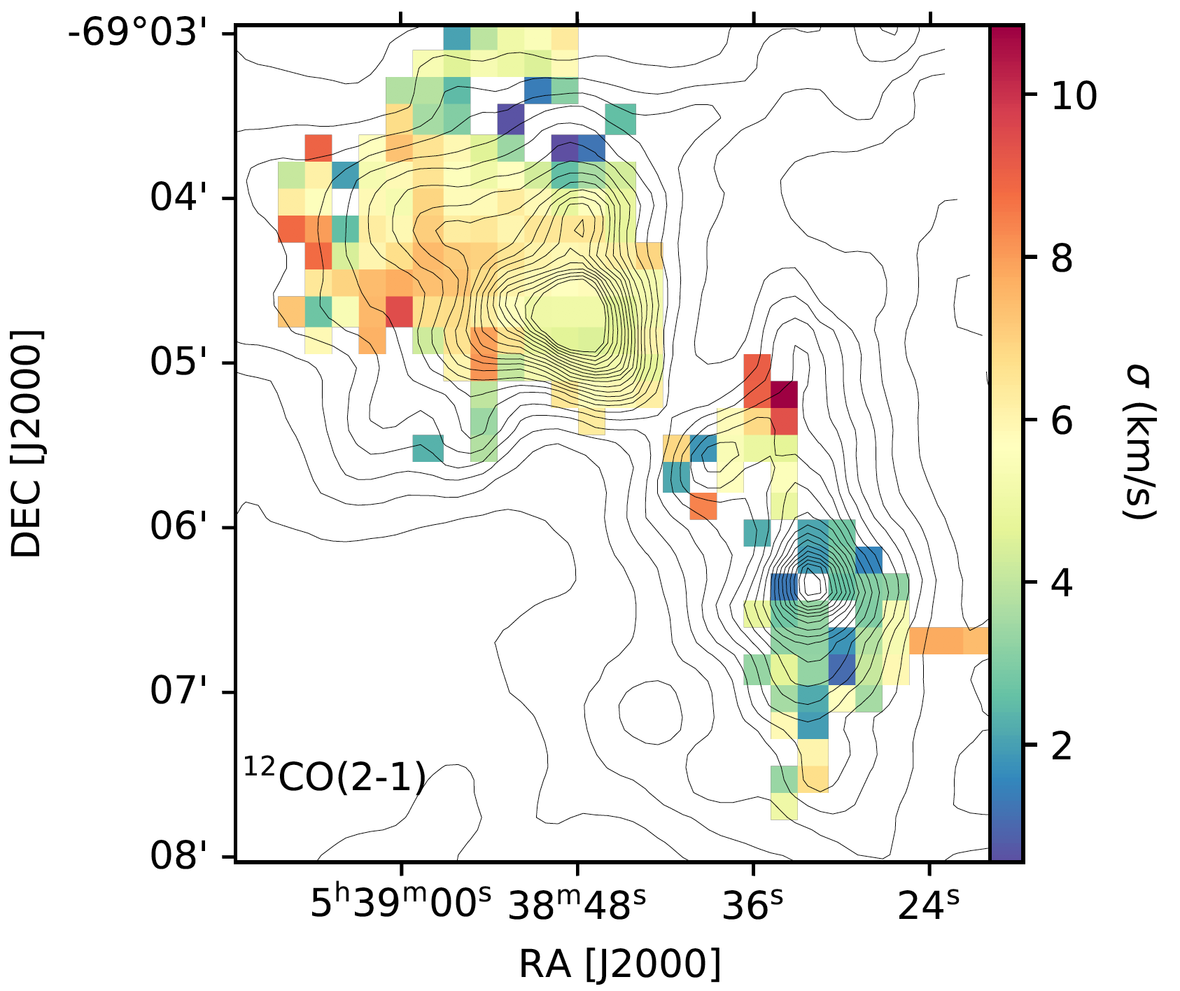
Figure 5: Upper Left: First-moment map obtained with the [CII] line. The black contours indicate the HAWC+ emission at 214 $\mu$m starting at 0.1 Jy pixel^-1 with increments of 0.1 Jy pixel^-1. The black arrows indicate the regions, with their name, for the position-velocity (PV) diagrams presented in Figure 6. The arrows indicate the increasing distance (d) in the PV diagrams. Lower left: The second-moment map of [CII]. Right: The same for ¹²CO(2-1).

In Okada et al. (2019) and Figure 3 several [CII] and CO spectra of 30 Dor are presented. These observations show that most of the emission is found between 220 and 280 km s^-1. In this velocity range, multiple velocity components and high-velocity wings are observed. In Figure 3, the wings are most clear in spectra 1-4 and specifically in the velocity range between 220-240 km s^-1 and between 255-280 km s^-1. Such wing-like structures were recently also found in spectrally resolved [CII] observations toward galactic HII regions (e.g. Schneider et al., 2018, 2020; Tiwari et al., 2021; Bonne et al., 2022a). The 30 Dor region has a complex dynamical structure. This is illustrated in more detail for [CII] and ¹²CO(2-1) in Figures 4 and 15 (in App. A). Despite the complexity of the kinematics and the fact that they trace different densities, Figure 4 shows that both lines have a broadly similar velocity structure on large scales. Inspecting the velocity structure in Figure 4, it can be noted in particular with [CII], that the blue- and red-shifted gas appear to create intersecting axes toward the middle of the SOFIA map. This intersection is shown in Figure 4 by the north-east to south-west axis for blue-shifted velocities and the east-to-west axis for red-shifted velocities. This intersecting structure formed by the blue and red axis is also observed in the channel maps of the region that are presented in Figure 15 of App. A. The channel maps also confirm that the southern part of the maps consists of two subregions, which are discontinuous in velocity. This is consistent with the HAWC+ integrated maps, which show that this western region contains two clumps. Furthermore, these two subregions have a noticeably different B-field structure in Figure 9. In the northern region of the map it is also observed that there is a noteworthy change in B-field orientation at the transition from blue- to red-shifted gas which confirms that the B-field morphology is directly related to the large-scale kinematics of the 30 Dor region, see Figure 4.

From the data cubes, the moment maps can be calculated. However, before presenting these moment maps, it has to be noted that there are limitations to the moment maps due to the inherent complexity (i.e., multiple components and high-velocity wings) in the spectra. The resulting moment maps are presented in Figure 5. The first-moment map (or the velocity field) has an organized gradient that looks similar in [CII] and ¹²CO(2-1) and fits with the velocity field obtained at smaller scales with ALMA observations (Indebetouw et al., 2013). Even though both lines show a similar morphology, it is found that the [CII] velocity field covers a significantly larger velocity range. The CO kinematics thus tend to follow the [CII] kinematics, but less drastically.
Both lines are expected to trace different regions in the cloud because of the critical density and the fact that FUV radiation propagates further into the cloud in low-metallicity regions. From the second moment maps, presented in Figure 5, it is observed that the linewidth significantly depends on the observed line. For this, it has to be taken into account that there are indications of multiple components, also reported in Melnick et al. (2021), which are particularly clear in [CII]. For example, two velocity components are prominent in the most north-eastern part of the map (see Figure 3), which is translated in a large second moment in that region. From the maps, it is also observed that the northern region has a higher second moment than the southern region, which could be related to the smaller velocity range covered by the velocity field in that region. Both lines do show a common behavior for the second moment over the map. Specifically, they show a reduction in linewidth towards the densest gas of the northern and southern regions.

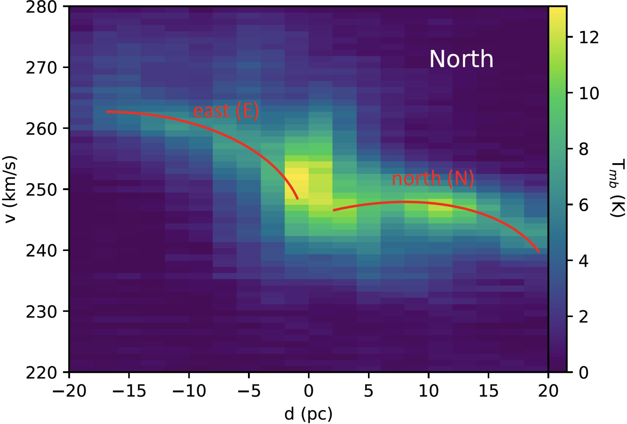
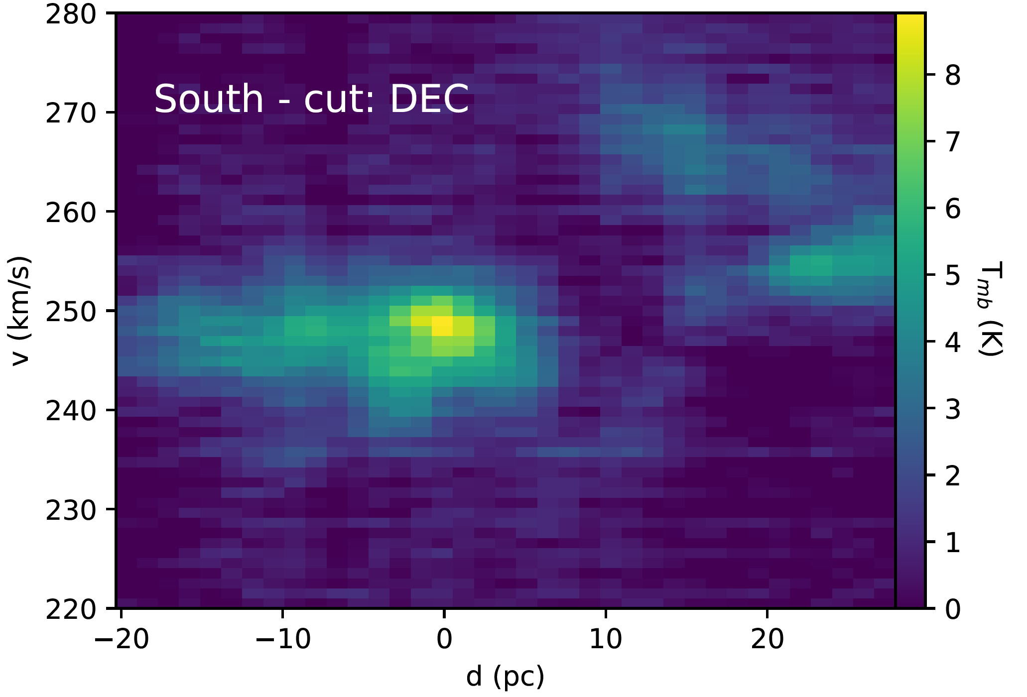
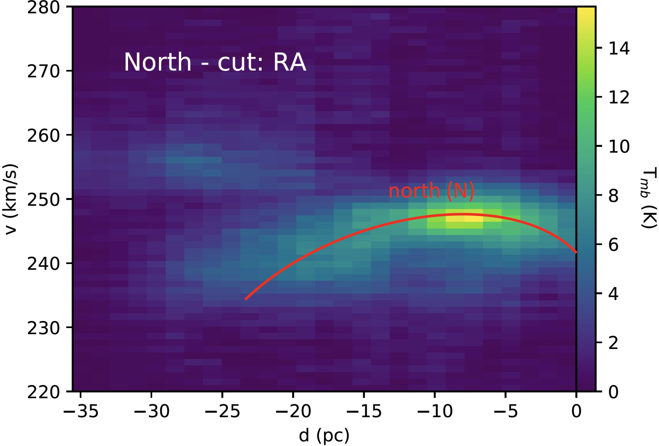
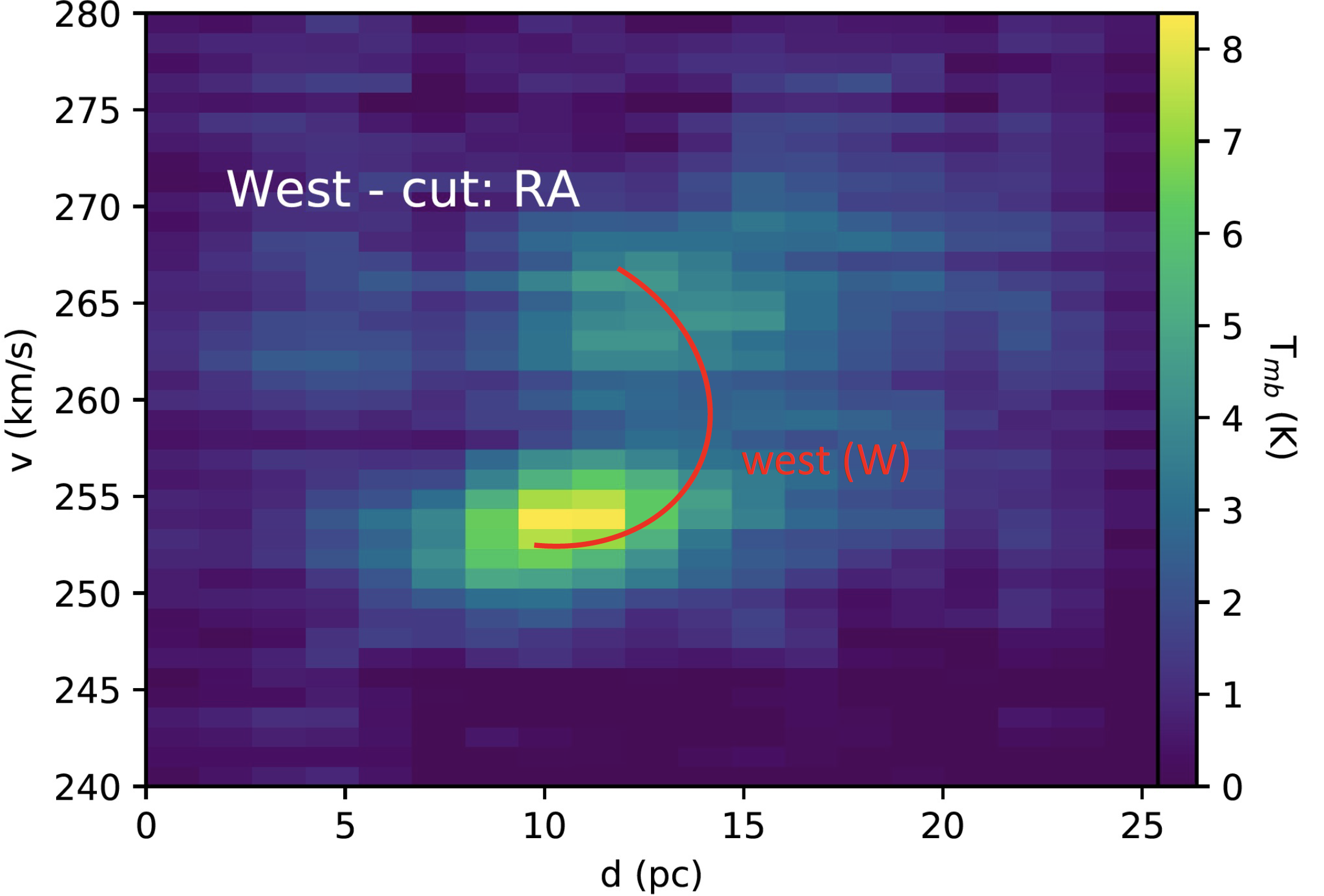
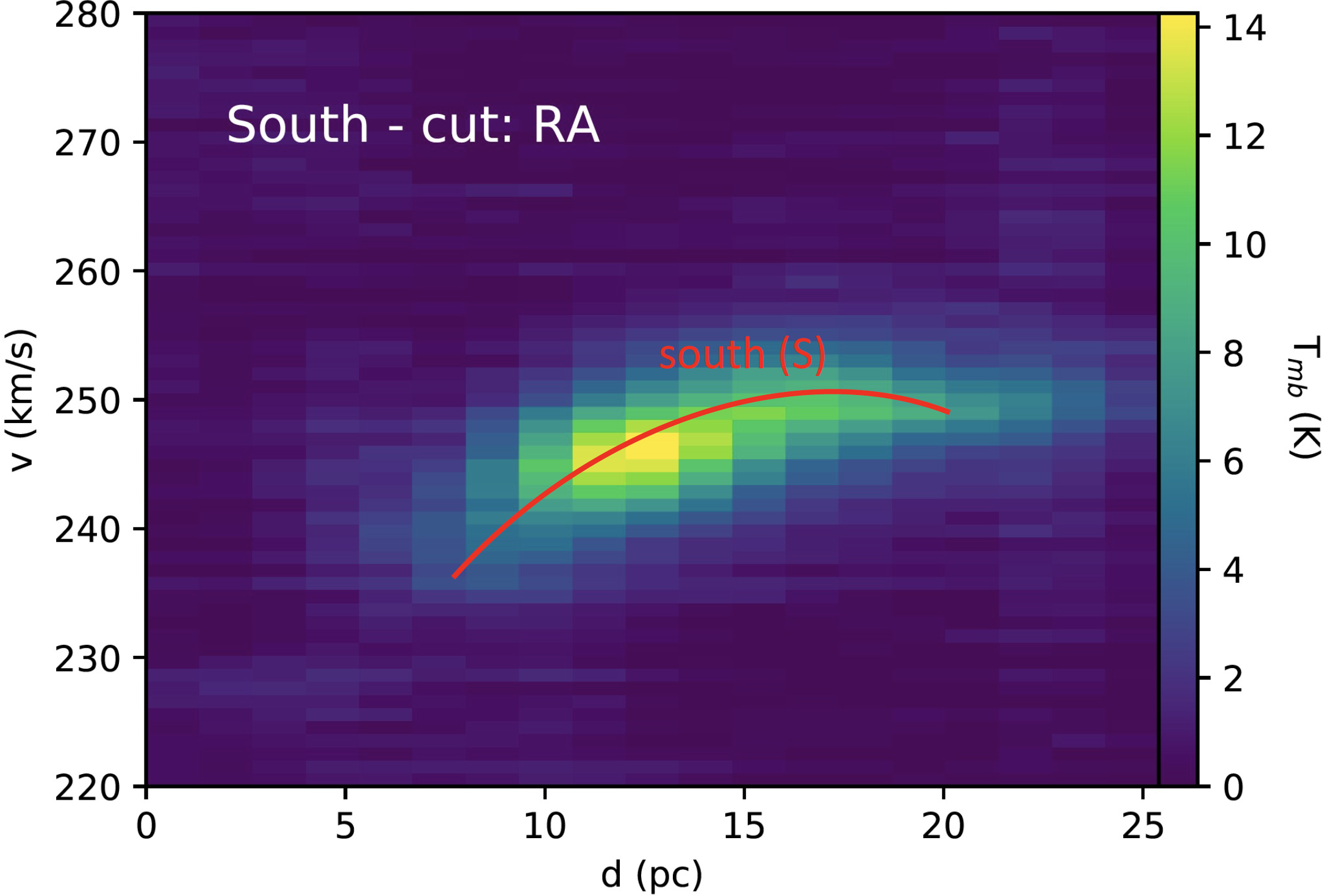
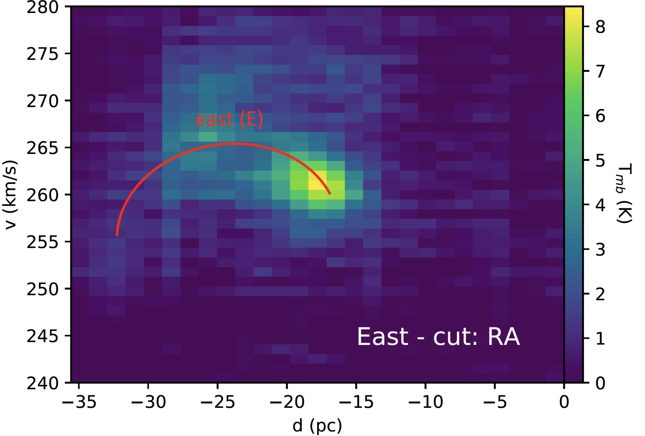
Figure 6: [CII] position-velocity diagrams, with a spatial resolution of $\sim$ 4 pc and a spectral resolution of 0.5 km s^-1, over multiple regions of the 30 Dor cloud at the locations indicated by the name in white. The cuts used to produce the PV diagrams in the top row are indicated in Figure 3 and the cuts used to produce the PV diagrams in the two bottom rows are indicated in Figure 5. All cuts show large gradients, often with a curve like nature, over 5-15 km s^-1 which could be associated with the presence of multiple expanding shells in this cloud. These candidate expanding shells, with their name, are indicated in red.

2.3 Position-velocity diagrams of 30 Doradus

The magnetic field observations of 30 Dor, presented in Figure 9 and Tram et al. (2021c), unveil a relatively organized structure in most regions of the cloud. As a result, it defines the main direction for both the northern clump and the southern regions of the map. This direction of the magnetic field in both regions will be used to study the [CII] kinematics of 30 Dor using position-velocity (PV) diagrams. These two directions, which are aligned with the mean field lines, are presented in Figure 3. Additionally, cuts through 4 regions in the RA direction were made for PV diagrams of [CII]. The location of these cuts is presented in Figure 5. All the resulting PV diagrams are presented in Figure 6.
These PV diagrams confirm that there are several organized velocity gradients in the region. These gradients cover a velocity interval of 5 - 15 km s^-1 in most PV diagrams and come in the form of curves/half-elliptical features that have been associated with expanding shells (Pabst et al., 2019, 2020; Luisi et al., 2021; Tiwari et al., 2021; Beuther et al., 2022; Bonne et al., 2022a). Based on the presence of these curved features, we identify 4 expanding shell candidates over the full map using the PV diagrams. The curved velocity structures associated with the candidate expanding shells are indicated in Figure 6. With the channel maps in Figure 15, we confirm that these candidates have a spatially curved/ring-like morphology as expected for expanding shell features. We name these candidate expanding shells: north, east, west, and south after their location on the map. The location and velocity range of these expanding shell candidates are presented in Table 1. The location of these shell candidates is also indicated over their velocity range in Figure 15. Two expanding shell candidates are found in the range of 230 to 250 km s^-1 and two are found in the range of 250 to 265 km s^-1. As some of these shells appear to be only partly covered, larger maps will be required to: study their full extent, better characterize their properties and investigate whether some of the identified shells have the same expansion origin or not. This will also help to study, in combination with data at different wavelengths, whether radiation or stellar winds drive these expanding shell motions. As the expanding shells are directly identified by the two blue and red regions in the RGB image in Figure 4, this shows that the magnetic field curvature is associated with these expanding [CII] shell candidates. The highest-density region in the northern region is located at the intersection of two expanding shells. It might be possible that this region is formed by the collision of the two expanding features. This could result in additional magnetic field bending through oblique shocks (e.g. Inoue & Fukui, 2013; Bonne et al., 2020b). However, in the complex dynamical structure, and with the limited spectral [CII] resolution, it is not easy to establish indications of such magnetic field bending with confidence. Additionally, the increasing role of gravity might also alter the magnetic field morphology in this high-density region.

Expanding shell candidates
location	$\alpha_{J2000}$	$\delta_{J2000}$	velocities (km s-1)
north (N)	05:38:55	-69:04:00	230-250
east (E)	05:38:55	-69:05:30	250-265
west (W)	05:38:32	-69:05:00	250-265
south (S)	05:38:32	-69:06:30	235-250

Table 1: The location and velocity range for the identified expanding shell features in the 30 Dor region.

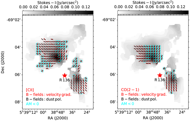
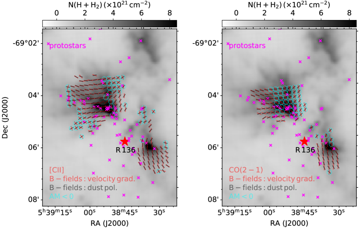
Figure 7: Comparison of magnetic fields inferred from the VGTs (red) and from the thermal dust polarization (black). The VGs estimated from [CII] are shown on the left, and from CO(2-1) on the right. The cyan circles indicate where these inferred magnetic fields are misaligned (i.e., the velocity gradient is parallel to the field lines). The background is the total dust intensity at $214\,\mu$m.

Figure 8: Same as Figure 8 but overlaid with the protostars adopted from Indebetouw et al. (2009). Interestingly, the protostars likely locate at which VGTs misalign with B-fields (i.e., VGs are parallel to the field lines).

2.4 Velocity gradient technique

In this section, we computed the velocity gradients of both [CII] and CO(2-1) from their channel maps adopted from Hu et al. (2021a), which is referred to as VChGs (Lazarian & Yuen 2018). Here we recall the principle of this method. The methodology follows these steps: (1) the initial Position-Position-Velocity datacube was pre-processed using principle component analysis by splitting a very large number of velocity channels along the LOS as long as the thin channel map criteria is satisfied (Lazarian & Pogosyan 2000); (2) the product was convoluted with a $3\times 3$ Sobel Kernel to create a raw gradient map (pixels are blanked out if their intensity is less than three times root-mean-square level); (3) the gradient angle at each pixel was statistically computed from an adaptive sub-block average method (Yuen & Lazarian 2017a), in which all single gradient orientation within a rectangle sub-block in the raw gradient map was taken into account; (4) the pseudo-Stokes Q and U of the gradient were created (Lu et al. 2020), which allows computing the velocity gradient morphology. As the principle of VGT, the magnetic fields are inferred from this technique by rotating the velocity gradient orientation by 90 degrees (González-Casanova & Lazarian 2017). However, please note that the zeros-angle of the velocity gradient is defined along the East-West direction, which is an offset angle of the polarization angle defined by the SOFIA/HAWC+. Therefore, the velocity gradient orientation naturally infers the magnetic fields in the frame of the SOFIA/HAWC+ thermal dust polarization.

Figure 8 shows the magnetic fields inferred by the VGTs (red vectors) from both [CII] (left panel) and CO(2-1) (right panel). To measure the correlation between B-fields inferred from VGTs and SOFIA/HAWC+ (black vectors), we computed the local alignment measurement (AM) as (González-Casanova & Lazarian 2017)

$$AM=2\left(\cos^{2}\theta_{r}-\frac{1}{2}\right)$$ (1)

with $\theta_{r}=|\theta_{\rm VG}-\theta_{\rm HAWC+}|$ the angle differences between VGTs and HAWC+. These two vectors are parallel when $AM=1$, while they become perpendicular once $AM=-1$. $AM<0$ indicates where these two vectors are misaligned (i.e., VGs are parallel to B-field lines). One can see that the VGT agrees well with the dust polarization in the South (i.e., VGs are perpendicular to B-field lines), but only fairly in the North. The VGT computed by [CII] shows that the misalignment occurs mostly at the edge of the regions where the gas density is not peaked (see the paper I). The VGT from CO(2-1) further shows that the misalignment occurs at the denser regions. The reason is that [CII] traces for more diffuse gas than CO so that it is less affected by gravity.

3 Magnetic fields in 30 Doradus

To map the B-fields of 30 Dor, we make use of the SOFIA/HAWC+ polarimetric data at 89, 154, and 214$\,\mu$m observed under the Strategic Director’s Discretionary Time (S-DDT) program (PI: Yorke, H., ID: 76$\_$0001) during the SOFIA New Zealand deployment in July 2018. The reduction of data was introduced in Gordon et al. (2018).

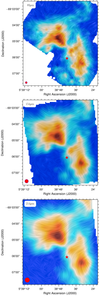
Figure 9: Magnetic field morphology in 30 Dor for all three bands (from top to bottom). The background is the total intensity stokes I. Streamlines are the LIC (Cabral & Leedom 1993). The Star symbol indicates the R 136 location.

3.1 Magnetic field morphology

Assuming grains are perfectly aligned with the B-fields, Figure 9 shows the geometry of the fields for all three bands (top to bottom), which is inferred from the polarization vectors. The background color is the original total intensity (Stokes I). One can see that there are two main regions in 30 Dor, these are North and South regions relative to the massive star cluster R 136, whose center is located by the red star. The B-fields are complex but highly ordered, and show a curved feature around the peak intensity (or the peak gas density) in both the North and the South regions. The field lines are curved toward the central cluster. In addition, the field structure at the East-side of the peaked intensity in the North region looks like an hourglass. These behaviors are observed similarly in all three bands. The discrepancy among the three panels shown in Figure 9 is mainly due to the fact that shorter wavelength has higher spatial resolution than longer ones.

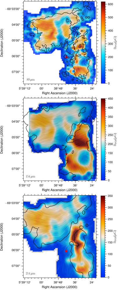
Figure 10: Maps of $B_{POS}$ strength for all three bands (from top to bottom) using [CII] overlaid with the B-field orientation. The black contours indicate the region where $I/\sigma_{I}\geq 100$ and $p/\sigma_{p}\geq 3$. The star symbol indicates the R 136 location. The B-field strength is weaker at longer wavelengths with peaks offset from the total intensity.

3.2 Magnetic field strength

The distortion of the B-field morphology could result from the local conditions. For example, this could possibly be explained by the compression of the magnetic field by turbulence, shock (Inoue & Fukui 2013), or gravitational contraction (Ewertowski & Basu 2013). To address which is a likely cause of this interesting situation, we thus estimate the map of the B-field strength.

We determine the spatial distribution of the POS magnetic field strength in 30 Dor according to the strategy developed by Guerra et al. (2021):

• A map of the strength of the magnetic field in the POS can be determined using the Davis-Chandrasekhar-Fermi (DCF; Davis 1951; Chandrasekhar & Fermi 1953), based on the equipartition of the turbulent magnetic energy and the turbulent kinematic energy, approximation:

  $$B_{\rm POS}\simeq\sqrt{4\pi\rho}\frac{\delta V_{\rm t}}{\delta\phi}$$ (2)

  where $\delta V_{\rm t}$ is a map of the velocity dispersion of the gas, $\rho$ is the map of the gas density and $\delta\phi$ is a map of the angle dispersion of the polarization orientation. Following a modification in Houde et al. (2009), the angle dispersion is replaced by the angular dispersion (or structure-function) proportional to the ratio of large-to-small scales magnetic energies as $\delta\phi\simeq[\langle B^{2}_{t}\rangle/\langle B_{0}^{2}\rangle]^{1/2}$. This improvement is able to avoid the spatial change in the magnetic field morphology with $\langle B_{t}^{2}\rangle/\langle B_{0}^{2}\rangle$.

• The structure-function dispersion analysis (Houde et al., 2009) was applied to every map of $\boldsymbol{B}$-field angles ($\phi$) in a pixel-by-pixel fashion. This means, for a given pixel $i$, a circular kernel of radius $w$-pixel is defined around it. All the pixels inside this kernel are then used to calculate the dispersion function $1-\langle\cos[\Delta\phi(\ell)]\rangle$ for pixel $i$. This dispersion function can be described by the two-scale model:

  $$1-\langle\cos[\Delta\phi(\ell)]\rangle=\frac{1-e^{-\ell^{2}/2(\delta^{2}+2W^{2})}}{1+\mathcal{N}\left[\frac{\langle B_{t}^{2}\rangle}{\langle B_{0}^{2}\rangle}\right]^{-1}}+a_{2}\ell^{2}.$$ (3)

  where $\Delta\phi(\ell)$ is the difference between a pair of $\phi$ separated by the distance $\ell$. The first term in Equation 3 describes the small-scale, turbulent $\boldsymbol{B}$ contribution to the dispersion. In this term, $\delta$ is the turbulence correlation length, $\mathcal{N}(=\Delta^{\prime}(\delta^{2}+2W^{2})/\sqrt{2\pi\delta^{3}})$ is the number of turbulent cells along the LOS, and $W$ is beam’s radius (e.g. the $\sigma$ value) of the polarimetric observations. $\Delta^{\prime}$–the cloud’s effective depth–is used as a proxy for the depth along the LOS (see Houde et al. (2009) for definition). The second term in Equation 3 quantifies the contribution from the large-scale, ordered magnetic field to the dispersion function.

• The dispersion function in every pixel is fitted with Equation 3 using a MCMC solver. This fitting process can determine values of $\langle B_{t}^{2}\rangle/\langle B_{0}^{2}\rangle$, $a_{2}$, and $\delta$ in every pixel. The map of $\langle B_{t}^{2}\rangle/\langle B_{0}^{2}\rangle$ is required to estimate the POS magnetic field strength.

• Before combining all three maps through Equation 2, they must have the same angular resolution. In order to do that, the lowest angular resolution (target resolution;$\sigma_{T}$) among $\delta V$, $\rho$, and $\langle B^{2}_{t}\rangle/\langle B_{0}^{2}\rangle$ is chosen and the other maps are smoothed using a Gaussian kernel with width $\sigma^{2}\xrightarrow{}\sigma_{T}^{2}-\sigma^{2}$.

The choice of kernel size, $w$, is important for the fitted values of ${\langle B_{t}^{2}\rangle}/{\langle B_{0}^{2}\rangle}$, $a_{2}$, $\delta$(if fitted), and therefore the $B_{\rm POS}$ maps. According to Guerra et al. (2021), the kernel size needs to be large enough to result in statistically-significant dispersion functions but small enough for any resulting map to have meaningful angular resolution and avoid smoothing them over large areas. The optimal kernel size, $w_{\rm opt}$, can be found by monitoring the distribution of $\rho$ values – between the constructed dispersion function and its fit in every pixel. We performed tests using the 214-$\mu{\rm m}$ map and values of $w$ = 7, 9, 11 pixels and found that $w$ = 9 pixels produced the largest fraction of pixels with $\rho\sim$1. Table 2 shows the values of $w_{\rm opt}$, global $\delta$, and correlated beam size ($\sqrt{2}W$) for all three bands. From these values, it is clear that the 9-pixel-radius circular kernel contains 7.5 correlated beams and 2 to 3 turbulence correlation lengths.

Using kernels with $w>w_{\rm opt}$ will not result in better-determined fitting parameters since the addition of more pairs of vectors will not modify the small-scale portion of the dispersion function. Instead, it will result in the contribution of scales larger than those described by the term $\propto\ell^{2}$ which are not described by the model in Equation 3.

In order to evaluate Eq. 2, we used the $N(\rm H_{2})$ map from Paper I and for $\delta V$ we used the second moment map of either CO or [CII] (Figure 5). To transform column density to mass density, the cloud’s depth must be used. In this work, we used the $\Delta^{\prime}$ defined above, which is calculated as the width of the auto-correlation function of the polarized intensity. However, taking into consideration that the 30 Dor complex is distinctly separated into two clumps, assuming one single value for $\Delta^{\prime}$ can result in less accurate values of $B_{\rm POS}$. Therefore, we created a map of $\Delta^{\prime}$ that consists of two areas (north and south) each with a constant, different value. These values are displayed in Table 2. On the other hand, the second moment ($\delta V$) calculated from CO and [CII] observations, contains contributions from thermal motions of the molecules as well as turbulent motions. Therefore, the velocity dispersion values were corrected as $(\delta V_{\rm t})^{2}=(\delta V)^{2}-k_{\rm B}T_{\rm gas}/m$, where $k_{\rm B}$, $T_{\rm gas}$, and $m$ are the Boltzmann constant, the gas temperature, and the molecule’s mass. In this work, we assume 30 Dor is in LTE condition and adopt $T_{\rm gas}=T_{\rm ex}$. We computed the excitation temperature $T_{\rm ex}$ at each pixel using its maximum main-beam temperature as in Pineda et al. (2008).

30 Dor

$\lambda$ [$\mu{\rm m}$]	$\delta$ [′′]	$\sqrt{2}W$ [′′]	$w_{\rm opt}$ [′′]
89	16.00	4.68	17.55
154	21.56	8.17	30.51
214	23.68	10.93	40.95

North

$\lambda$ [$\mu{\rm m}$]	$\Delta^{\prime}$ [arcmin]	$\Delta^{\prime}$ [pc]
89	0.55	7.84
154	0.74	10.53
214	0.76	10.82

South

$\lambda$ [$\mu{\rm m}$]	$\Delta^{\prime}$ [arcmin]	$\Delta^{\prime}$ [pc]
89	0.33	4.70
154	0.40	5.70
214	0.38	5.41

Table 2: Values of turbulence correlation length ($\delta$), correlated beam size ($\sqrt{2}W$), and optimal kernel size ($w_{\rm opt}$) for the map-making procedure (Top). Cloud’s effective thickness ($\Delta^{\prime}$) for the north (middle) and south (bottom) regions of 30 Dor. These values were calculated as the half-width half-max of the one-dimensional auto-corrrelation of the polarized flux at each wavelength. Linear depths are calculated from angular depths assuming a distance of 49 kpc.

According to Guerra et al. (2021), there are two alternatives to fitting the dispersion function (see their Appendix A): 1) solving for all three parameters ($a_{2},{\langle B_{t}^{2}\rangle}/{\langle B_{0}^{2}\rangle},\delta$) simultaneously. If this provides the majority of pixels in the map with values of $\delta$ greater than $\sqrt{2}W$, then the turbulent contribution is well resolved by the polarimetric observations and the values of ${\langle B_{t}^{2}\rangle}/{\langle B_{0}^{2}\rangle}$ are well-defined. 2) If the condition $\delta>\sqrt{2}W$ is not met for the majority of pixels, the parameter $\delta$ can be fixed to a prescribed value and the MCMC solver computes only two parameters, $a_{2},{\langle B_{t}^{2}\rangle}/{\langle B_{0}^{2}\rangle}$. For this investigation, the first approach was tried with all polarimetric maps, but only the 214-$\mu{\rm m}$ satisfied the condition mentioned above. For the results here presented we used the second approach, with a prescribed $\delta$ value for each pixel equal to that from the global analysis (e.g. when only one dispersion function is calculated for the entire observation). Using the $\delta$-fixed approach results in underestimated values of ${\langle B_{t}^{2}\rangle}/{\langle B_{0}^{2}\rangle}$ and overestimated values of $B_{\rm POS}$. However, a test performed with the 214-$\mu{\rm m}$ data (the only map for which $\delta>\sqrt{2}W$ was met in the majority of pixels) showed that differences in $B_{\rm POS}$ values using these two approaches were small, with an average value of $\sim$16%.

The resulting maps of $B_{\rm POS}$ strength, calculated using the [CII] data, are presented in Figure 10 for all three bands 89, 154, 214 $\mu{\rm m}$ (from the top to bottom). These maps have angular resolutions of 33^′′, 58^′′, 77^′′, respectively. The estimated strengths show a dependency with the wavelength of the polarimetric data. Values range between few and $\sim$350, $\sim$450, and $\sim$600 $\mu$G for 214, 154, and 89 $\mu{\rm m}$. This wavelength discrepancy should be mainly because of the angular resolution of the map – shorter wavelengths have smaller resolution. However, there is also a possibility that such differences are the result of each individual wavelength tracing different layers of the cloud. At the same wavelength, the strength structure using CO is similar to the one using [CII], but the amplitudes are slightly lower (see Appendix B). The uncertainty of our calculation is discussed in Section 4.5. The black contours in Figure 10 indicate the spatial area in which $I/\sigma_{I}\geq 100$ and $p/\sigma_{p}\geq 3$ (e.g., the polarization measurement is statistically significant and intrinsically associated with the source as discussed in Paper I).

3.3 Magnetic fields vs. gravity

An important factor indicating the influence of the magnetic field is the mass-to-flux ratio. We adopt the ratio as in Crutcher et al. (2004) as

$$\lambda=7.6\times 10^{-21}\frac{N({\rm H}_{2})}{B_{\rm tot}}$$ (4)

where $B_{\rm tot}=\sqrt{B^{2}_{\rm POS}+B^{2}_{\rm LOS}}$ in $\mu$G is the strength of the magnetic field in three-dimension, which is missing in this work because we do not have the LOS component of the field, and $N_{\rm H_{2}}$ in $\rm cm^{-2}$ is the gas column density. Statistically, $\overline{B}_{\rm tot}$ could be approximated as $4/\pi\times\overline{B}_{\rm POS}$ (Crutcher et al. 2004). Using the measured Zeeman LOS component of the field, Guerra et al. (2021) showed that $B_{\rm tot}\simeq B_{\rm POS}$ in the specific case of OMC-A (see their Equation 11 and Table 1). Lacking information on the LOS component, we simply adopt $B_{\rm tot}=B_{\rm POS}$ with the same caveat as many other studies (e.g., Soam et al. 2018b; Eswaraiah et al. 2021; Ngoc et al. 2021; Hoang et al. 2021b). The gas column density is derived by a modified black-body fitting from Herschel data at 100, 160, 250, 350, and 500$\,\mu$m (Meixner et al. 2013) as in Paper I. The cloud is called supercitical for $\lambda>1$, in which the magnetic field is insufficient to provide support against the gravitational potential. Otherwise, the cloud is called subcritical for $\lambda<1$ in which the magnetic field prevents the cloud from collapsing.

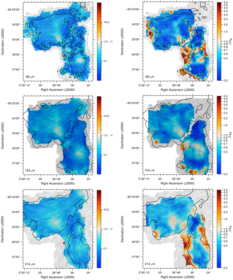
Figure 11: Maps of the mass-to-flux ratio (left panels), and the Alfvénic Mach number (right panels) for all three bands (wavelength increases from top to bottom) overlaid with the fields morphology. The black contours border is defined where $I/\sigma_{I}\geq 100$ and $p/\sigma_{p}\geq 3$. The red star indicates the R 136 location.

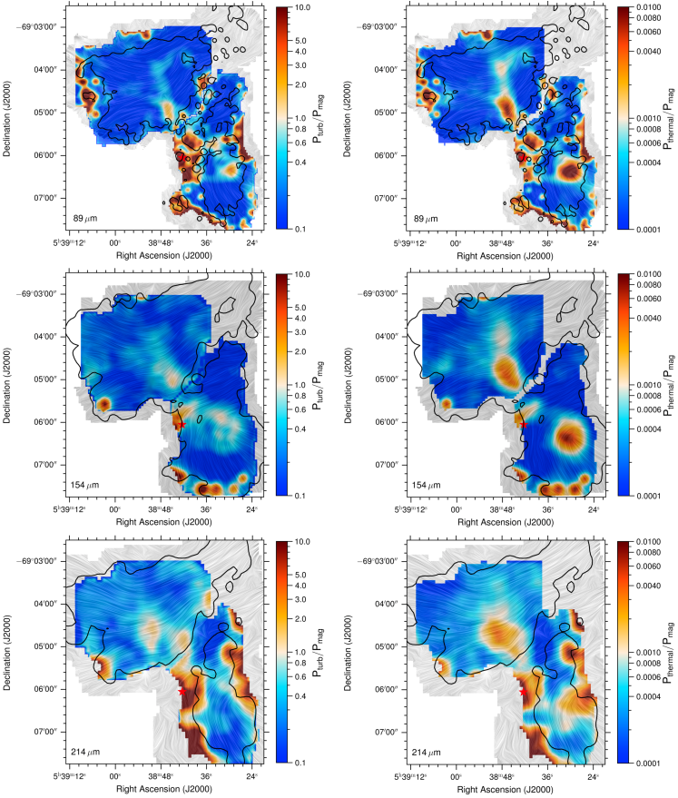
Figure 12: Turbulent-to-magnetic pressure ratio (left panels) and thermal-to-magnetic pressure ratio (right panels). The symbols are the same as in Figure 11. The magnetic pressure is higher than that of the turbulence everywhere across the cloud except in the peak intensity and the Eastern edge in the North where the turbulent pressure is higher or comparable to the magnetic pressure at the peak intensity in the North and South regions. The magnetic pressure is dominating the thermal one over the cloud.

Figure 11, left panels show the maps of the mass-to-flux ratio for all three bands (from top to bottom) overlaid with the field lines. Generally, the cloud is sub-critical ($\lambda<1$) for most of the region, except at the peak intensity in both the North and South ($\lambda\geq 1$), and the regions where $\lambda\sim 1$ spreads larger in area at longer wavelengths. Since $\lambda\sim N(\rm H_{2})$, and $B_{\rm pos}\sim\sqrt{N(\rm H_{2})}$, the gas density is the main uncertainty factor, which is discussed in Section 4.5. Our derivation of $N(\rm H_{2})$ agrees quite well with the one from PDR models (Chevance et al. 2020). As the maximum of gas column density is about $10^{22}\,\rm cm^{-2}$, a hundred $\mu$G B-field can make $\lambda<1$ (see Equation 4).

3.4 Magnetic field vs. Turbulence

The interplay between the B-field and turbulence can be defined through the Alfvénic Mach number. Because the DCF assumes that the turbulent magnetic energy balances the turbulent kinematic energy, the total magnetic energy estimated by the DCF method always greater than the turbulent kinematic energy, which leads to an Alfvénic Mach number is always lower than 1. Therefore, we use the 3D Alfvénic Mach number to assess the relative importance between the magnetic field and turbulence as

$$\mathcal{M}_{A}=\sqrt{3}\frac{\sigma_{\rm NT}}{\mathcal{V}_{A}}$$ (5)

where $\sigma_{\rm NT}$ is the non-thermal velocity dispersion, and $\mathcal{V}_{A}=B_{\rm tot}/\sqrt{4\pi\rho}$ is the Alfvénic velocity. $\mathcal{M_{A}}<1$ stands for the sub-Alfvénic, the impact of the gas turbulence is minimal and the magnetic fields are able to regulate the gas motion. $\mathcal{M_{A}}>1$ stands for the super-Alfvénic, the gas turbulence drives the magnetic fields to be random fields.

The right panel in Figure 11 shows the map of the Alfvénic Mach number in three bands (from top to bottom). These maps are color scaled such that the blue-color represents $\mathcal{M}_{A}<1$ and the red-color is for $\mathcal{M}_{A}>1$. One can see that the entire cloud is made up of sub-Alfvénic motions, while it is trans- or super-Alfvénic at around the peaked intensity both in North and South, except at 214$\,\mu$m where the the South peak becomes sub-Alfvénic. Similar to mass-to-flux ratio maps, the trans-Alfvénic area is more widespread at longer wavelength.

The magnetic and isotropic turbulent pressures in units of $\rm dyn\,cm^{-2}$ are computed as

$$P_{\rm mag} = \frac{B_{\rm tot}^{2}}{8\pi}$$ (6)

$$P_{\rm turb} = \frac{3}{2}\rho(\sigma_{\rm NT})^{2}$$

If $P_{\rm turb}/P_{\rm mag}$ is greater than 1, the turbulence pressure is higher than the magnetic pressure, otherwise the magnetic pressure is dominant. The maps in all three bands are shown in the left panels of Figure 12, indicating that the turbulent pressure is comparable and higher than that of the B-field at which $\mathcal{M}_{A}\gtrsim 1$, elsewhere it becomes lower (see Figure 11, right panels).

3.5 Magnetic vs. thermal pressure

The relative importance between the magnetic and thermal pressure could be quantified through a so-called plasma beta parameter, which is a ratio of these two pressures as

$$\beta=\frac{P_{\rm thermal}}{P_{\rm mag}}=\frac{2c^{2}_{s}}{\mathcal{V}^{2}_{\rm A}}$$ (7)

where $c_{s}=\sqrt{k_{B}T_{\rm gas}/\mu_{\rm H_{2}}m_{\rm H}}$ is the thermal sound speed. Figure 12, right panels show the maps of the thermal to magnetic pressure ratio. The magnetic pressure is much stronger than the thermal one and varies across the cloud, which is confirmed by the constraints observed by Lee et al. (2019) and Chevance et al. (2020) using the PDR Meudon code. Indeed, the authors constrained that $P_{\rm thermal}\sim 10^{4}-10^{6}\,\rm K\,cm^{-3}$, while we showed that $P_{\rm mag}\sim 10^{7}-10^{8}\,\rm K\,cm^{-3}$ with $B=200-500\,\mu$G.

4 Discussions

4.1 Gas column density probability distribution and turbulent driving force

The interplay between the gravity, magnetic fields and turbulence in the star-formation has been raised and discussed in numerous studies. The probability density function (PDF) of the gas column density was demonstrated to be a key to study the dynamics of molecular clouds. The PDF density of the isothermal and non-self-gravity gas follows closely a log-normal distribution; while this PDF develops a power-law tail once the self-gravity dominates and the collapse is significant (e.g., Klessen 2000; Federrath & Klessen 2013; Kainulainen et al. 2014; Girichidis et al. 2014; Schneider et al. 2013, 2015; Schneider et al. 2022).

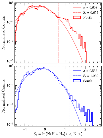
Figure 13: PDF distribution of the logarithm of the gas column density in the North (upper) and in the South (lower). A log-normal just fits up to $S_{t}\simeq 0.657$ (North) or $S_{t}\simeq 1.239$ (South), which are followed by a power-law tail. Apparently, the tail-structure in the North appears at lower gas density than in the South.

However, the shape of the PDF strongly depends on the way observations are performed as studied in Körtgen et al. (2019). The authors demonstrated that small or insufficient field-of-view will result in a cut-off in the log-normal part of the distribution, and argued that a sufficiently large field-of-view is needed for the PDF to be built completely. Thus, we used the whole column density map to build the PDF in Figure 13. Then, we fit a log-normal to the histogram as shown by the solid lines. One can see that a log-normal could not fit entirely the PDFs of both North’s and South’s gas density, but up to $S_{t}\simeq 0.657$ or $N\geq 1.8\times\bar{N}_{\rm North}=3\times 10^{21}\,\,{\rm cm}^{-2}$ in the North (upper panel), and $S_{t}\simeq 1.239$ or $N\geq 3.5\times\bar{N}_{\rm South}=3.8\times 10^{21}\,\,{\rm cm}^{-2}$ in the South (lower panel). Above these values, power-law tails can be seen in both regions. This reveals that the gravitational instability likely sets in relatively low gas density in 30 Dor cloud in general, and the North experiences it at a slightly lower density than that of the South because its power-law tail pops up earlier. The gravitational collapse in parsec-scale has been proposed in various studies (e.g., Hartmann & Burkert 2007; Peretto et al. 2006, 2013; Schneider et al. 2010; Jackson et al. 2019; Bonne et al. 2022b). Another note is that the gravitational collapse in the South is much more compact than in the North.

Figure 8 shows the location of the protostars candidates adopted from Indebetouw et al. (2009). These locations span from low to the peak gas column density. Interestingly, the protostars locations are coincident with the misaligned vectors between the rotated VGs by [CII] and CO and the B-fields, or at which these gas motions are parallel to the field lines.

The power-law tails have been seen to develop even in low column density gas, and we suspect that the turbulence could be the key gradient to make that happened. There are three main turbulent types, i.e., compressive (curl-free), solenoidal (divergence-free) and the mixing, in which the compressive turbulence results in stronger compression and thus larger deviation of the PDF (Federrath et al. 2010). These three types of turbulence could be identified through the turbulence driving parameter $b$ defined as

$$b^{2}=\frac{e^{\sigma^{2}}-1}{M^{2}_{S}}\frac{\beta+1}{\beta}$$ (8)

where $M_{S}$ is the sonic Mach number, $\sigma$ is the standard deviation of the log-normal distribution in Figure 13, $\beta=2M^{2}_{A}/M^{2}_{S}$ is the compressibility (or the plasma beta parameter in the right panel of Figure 12) with $M_{A}$ the Alfvenic Mach number. Purely solenoidal driving has $b=1/3$, the compressive driving turbulence yields $b=1$, and a stochastic forcing mixture has $b\sim 0.4$ (Federrath et al. 2010). Table 3 shows the mean values in the North and South regions. One can see that $b\simeq 1$ in both regions, which indicates that the driving force of turbulence in 30 Dor is mainly compressive. This is consistent with the existence of the supersonic expanding shells within the cloud discussed in Section 2.3, and similar to other star-forming regions; such as Serpens cloud (Hu et al. 2021a).

turbulent driving force
North region
band	$\bar{T}_{\rm gas}$	$\bar{\mathcal{M}}_{\rm A}$	$\bar{\sigma}_{v}$	$\sigma$	$\bar{b}$
C	31.68	0.41	8.46	0.608	1.15
D	31.68	0.46	8.46	0.608	1.03
E	31.68	0.61	8.46	0.608	0.78
South region
C	30.68	0.56	7.60	0.535	0.73
D	30.68	0.52	7.60	0.535	0.78
E	30.68	0.62	7.60	0.535	0.66

Table 3: Mean values of $\bar{b}\simeq 1$ in both North and South regions indicates that the turbulence in 30 Dor is likely the compressive driven.

4.2 Can Star-formation occur even in the strongly magnetized environment of 30 Doradus?

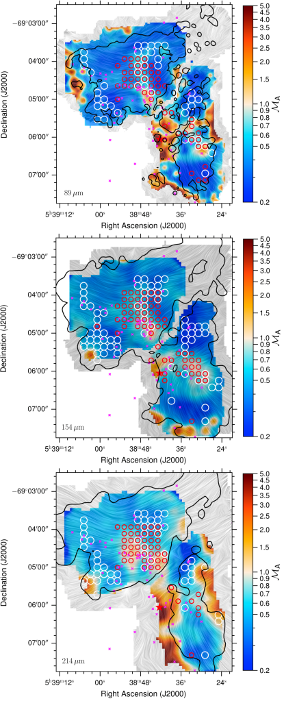
Figure 14: Alfvénic Mach number as shown in right panel of Figure 11. The white and red circles mark the positions where VGs from CII and CO are parallel to the fields (i.e., misaligned between VGT and magnetic field lines as shown in Figure 8), respectively. The magenta symbols show the locations of the protostars.

Figures 8 and 14 show that the velocity gradients of both CII and CO misalign with the B-fields at certain locations in both North and South regions, which indicates that (1) gas moves parallel to the field lines and (2) there is gravitational collapse. However, these positions distribute from low to maximum gas density, and mostly in magnetically sub-critical, sub-Alfvénic regions where the magnetic pressure is higher than that of the turbulence and thermal. The PDF of gas density in Figure 13 illustrates the power-law tail, an indicator of star-formation activities, at not very dense gas (column density few times higher than $10^{21}\,\rm cm^{-2}$) supporting the local collapse scenario, where protostars candidates are likely to locate. How can we explain the on-going star-formations in strong B-fields?

The turbulence driving parameters $b\simeq 1$ (see Table 3) reveals that the turbulence is mainly driven by compressive forcing in 30 Dor. The plasma parameter $\beta\ll 1$ (see Figure 12, right panel) shows that the sonic Mach number $\mathcal{M}_{s}\gg 1$, indicating the presence of supersonic turbulence. The supersonic compressive turbulence could create overdense gas in which the gravity gets unstable and stars can form by directly compressing the gas and/or accumulating the gas along the B-fields line. The latter will not be affected by the magnetic pressure because this pressure acts preferentially perpendicular to the field lines. As a result, the supersonic compressive turbulence could help to trigger the gravitational collapse. That turbulence could result from the cluster-wind from R 136 (Melnick et al. 2021) or probably the interaction with much larger giant HI-bubbles in the LMC (Kim et al. 1999). After that, the B-fields get amplified and slow down the star-formation activities, as we observe today.

4.3 Role of magnetic fields in holding 30 Dor integrity?

30 Dor contains a spectacular feature with multiple large expanding-shells (see Figure 1). The kinematic of these structures is just about $10^{50}-10^{51}\,\rm ergs$ (Chu & Kennicutt 1994), which could be generated by a cluster-wind (Melnick et al. 2021) or a combination with supernovae (Chu & Kennicutt 1994) from R 136. Melnick et al. (2021) estimated the virial mass within a distance of 25 pc from R 136 as a few times of $10^{6}\,M_{\odot}$ which is larger than the mass of 30 Dor gas (a few times of $10^{5}\,M_{\odot}$). Pellegrini et al. (2011) demonstrated that the thermal pressure (in order of $10^{-9}\,\rm dyn\,cm^{-2}$) is about 1.6 times lower than that of the radiation pressure (see their Figure 18), and is about 3 times higher than the hot gas pressure (i.e., the hot gas pressure is higher elsewhere, see their Figure 21). Thus, how can the 30 Dor cloud survive?

We suspect that B-fields play a crucial role here in holding the cloud integrity. The B-field morphology orients perpendicular to the radiation direction, so that the magnetic pressure could resist pressure coming from this direction. Indeed, the magnetic pressure is $P_{\rm mag}\simeq 1.6\times 10^{-9}-10^{-8}\,\rm dyn\,cm^{-2}$ for $B=200-500\,\mu$G, which is absolutely higher than both thermal and radiation pressure and thus is capable to resist against the radiative impact. This calculation is in agreement with the right panel in Figure 12. The role of B-fields could be deduced from a kinematic point of view. Melnick et al. (2021) showed that the kinematic energy of the region within 25pc from R 136 is about 24$\%$ the total kinematic energy (which is equivalent to $\simeq 5\times 10^{50}\,\rm ergs$). For $B=200-500\,\mu$G, the magnetic energy is orders of magnitude larger as $\simeq 10^{51}-2\times 10^{52}\,\rm ergs$ within the same spherical volume. In addition, Melnick et al. (2021) showed the turbulent kinematic energy could be up to $10^{51}\,\rm ergs$; thus, the turbulence only dominates over the B-field for $B<200\,\mu$G which is consistent with the maps of $\mathcal{M}_{A}$ (right panel in Figure 11) and $P_{\rm turb}/P_{\rm mag}$ (left panel in Figure 12).

The next question could be how large external shells developed around our cloud? 30 Dor opens to the Eastern direction from R 136, which helps hot gas (traced by X-ray, see Figure 14 in Townsley et al. 2006) easily escape and creates the large expanding-shell along this direction. The mechanism could otherwise be complicated along other directions, especially Northern and Western. There are multiple expanding-shells on a smaller scale within the cloud (see Figure 6) referring to the fact that the cloud is being carved by the cluster feedback. Melnick et al. (2021) proposed that this impact could lead the certain cloud’s structure to break, which enables hot gas to go through and ”inflate” the external expanding-shells along these directions. Interestingly, Figure 10 shows that the B-field strength is relatively weak (i.e., lower than 200$\,\mu$G) at certain regions in 30 Dor along directions that point to or adjoin to these external structures. Along these directions, the field is insufficient to resist feedback; thus, there are nozzles where the hot gas can escape through the cloud.

4.4 Comparison with the larger scale magnetic field of the hosting LMC

The larger-scale B-fields have been measured using both near-infrared (NIR) (e.g., Nakajima et al. 2007; Kim et al. 2016) and radio polarimetric observations (e.g., Klein et al. 1993; Mao et al. 2012).

The absorption polarization at NIR probed the B-field structure outside our region (see Figure 3 in Nakajima et al. 2007). These large field lines are seen to associate with the dust cloud in LMC and the large expanding structures around 30 Dor. The B-field strength from this more diffuse region was estimated of $3-25\,\mu$G using DCF.

The B-fields measured by synchrotron polarized emission inferred the larger scale of LMC. The low spatial resolution (e.g., $14^{\prime}$ in Mao et al. 2012) was unable to resolve our region. The total B-field strength is measured of $<7\,\mu$G, assuming equipartition with cosmic-ray electrons, with an upper-limit B-field on POS of $11\,\mu$G in the HI southwestern filaments up to the 30 Dor region. The higher B-field strength in the filaments may be due to anisotropic turbulent B-fields mostly located in POS.

Our B-field strengths of $350-600\,\mu$G at pc-scales using thermal dust polarization are much higher than the NIR and radio polarimetric observations in more diffuse media, which may be enhanced due to turbulent dynamo mechanism and star formation activity. The additional larger FIR and higher spatial resolution radio polarimetric observations of the LMC are required to better understand the connection between galactic B-fields and those B-fields responsible for the star-formation activity and molecular cloud formation.

4.5 Uncertainties

In this section, we discuss several possible uncertainties. Our first concern lies in the estimate of the column density, which is constructed by the modified SED fitting from Herschel data (see Paper I). Our derived column density agrees well in a range of $1.9\times 10^{21}-1.3\times 10^{22}\,\rm cm^{-2}$ estimation from PDR modelling (Chevance et al. 2020), but $1.3\times 10^{22}\,\,{\rm cm}^{-2}$ is 1.12 times higher than our maximum derivation. Hence if $B_{\rm pos}\sim N(\rm H_{2})^{0.5}$, the mass-to-flux ratio $\lambda$ increases by a factor 1.06, and the Alfvénic Mach number correspondingly decreases by a factor of 0.94, the magnetic pressure increases by a factor of 1.12. The values are slightly changed but do not affect our conclusions.

Our second concern is related to the volume density derived from the column density. The depth of the cloud is fixed and estimated by the auto-correlation function from the polarized intensity. Thus, our derived volume density is insensitive to the local cloud depth, which could be either over-/under-estimated.

The third concern is the non-thermal velocity dispersion. We computed this term by using [CII] and ¹²CO emission lines. These lines are not necessarily optically thin and show multiple components; hence it is not ideal for probing the turbulence component of the gas motion even though it shows no evident signs of absorption. If these emissions are optically thick, the non-thermal velocity dispersion might be overestimated because ($\delta V_{\rm turb})^{2}\sim(\delta V)^{2}$, (e.g., Phillips et al. 1979; Hacar et al. 2016).

The fourth concern is the gas temperature, because ($\delta V_{\rm turb})^{2}\sim(\delta V)^{2}-k_{\rm B}T_{\rm gas}/m_{\rm gas}$. We assume the gas is in the LTE condition, so we adopt $T_{\rm gas}=T_{\rm ex}$ across the entire cloud. This assumption will fail at the locations where the LTE is simply incorrect. However, we expect that $T_{\rm gas}$ has a little impact on the final result because (1) the thermal contribution is relatively small ($\simeq 2.6\,\rm km\,s^{-1}$ for $T_{\rm gas}=10^{4}\,{\rm K}$) compared to the total velocity dispersion (Figure 5), and (2) this velocity dispersion is supersonic for [CII].

The fifth concern is the strength of the B-field in 3D space. In this work, we adopt the value of the POS component of B-field since its LOS component is unknown in 30 Dor. The higher value of the total B-field strength will result in lower values of $\lambda$, $\mathcal{M}_{A}$, while increased in $P_{\rm mag}$. Chen et al. (2019) proposed a method to estimate the inclination of B-fields by assuming a uniform B-fields (i.e., no variation in position angle and inclination of the field lines) and a constant polarization coefficient (i.e., $p_{0}$ in their Equation 10) throughout a cloud. These assumptions are unlikely to be satisfied in the case of 30 Dor given a variation of the field lines and the polarization degree across the cloud.

The sixth concern is the method to estimate the B-field strength. In this work, we use an improved version of the DCF method from Houde et al. (2009), in which the structure-function of polarization angle is used rather than the dispersion function of this quantity. Skalidis & Tassis (2021) and Skalidis et al. (2021a) showed that the strength of the mean B-field component is proportional to $1/\sqrt{\delta\phi}$ which is different from Equation 2. However, this approach assumed an equipartition between turbulent motions and the parallel component of turbulent B-fields whose physical basics behind is not clear (see Appendix A3 in Li et al. 2022 and Section 10.3 in Lazarian et al. 2022). Recently, at the time of this work, Lazarian et al. (2022) proposed a new method to estimate the field strength, namely differential measure approach (DMA) as $B\simeq f\sqrt{4\pi\rho}D^{1/2}_{v}/D^{1/2}_{\phi}$ where $D_{v}$, $D_{\phi}$ are the structure functions of the velocity centroids and polarization angle, and $f$ is the factor based on the anisotropic turbulence. The authors showed that the DMA method could estimate the field strength at the smallest scale (lower than the turbulence injection scale) and with anisotropic turbulence properties. These two modifications contrast the DCF method and could increase the estimation accuracy. A comparison between DCF and DMA is beyond the scope of this work, and it hence serves as an important improvement for future works (not only for 30 Dor but also other star-formation regions).

To summarize, the quantitative value of B-field strengths could be different from what is presented in this work once using a proper value of the non-thermal velocity dispersion and the gas temperature for the DCF or different methods. However, it could not change by orders of magnitude, and we do not expect it will change the effect of the B-field. Indeed, when the strength is as high as hundreds $\,\mu$G, the field is strong enough to support against the gravitational potential (Equation 4) and is sufficient to resist the hot gas and radiation pressures (Section 4.3).

5 Conclusions

The entire 30 Dor is a complex star-forming region, which clearly shows a core-halo structure, in which there are multiple pc-scale expanding-shells structures in the outer region and a cloud in the inner region. Cluster-wind or a combination of supernovae from the star cluster R 136 is demonstrated to be the main source of energy for these giant shells (Chu & Kennicutt 1994; Melnick et al. 2021). However, it is not very clear how an inner structure is able to remain close to this source of energy. Thus, we study the gas kinematics and B-fields in this region in this work, for which we use the same name as 30 Dor for the sake of convenience. Our main findings are summarized as follows.

• We derived the B-field morphology from thermal dust polarization observed by SOFIA/HAWC+, which shows the highly ordered yet complex B-field structure. The field lines are wrapped and bent around the peak intensity (where the gas is densest, Figure 9). The tip of the bending fields points towards the star cluster, R 136.

• We performed velocity field analysis on two different gas tracers. One is expected to trace warmer and more diffuse gas ([CII]), and the other cold and dense gas (CO). Our analysis indicates a complex dynamic structure but organized with multiple gas components and wing-like structures. The change from the blue- to red-shifted gas is directly related to the B-field morphology change. Furthermore, the position-velocity diagrams showed possible multi expanding-shells in 30 Dor.

• We compared the B-fields obtained using the VGT of both [CII] and CO and showed that the B-fields mostly align with the one inferred from thermal dust polarization observed by SOFIA/HAWC+ in the South, while in the North, numerous misalignment vectors are seen (Figure 8). CO line shows anti-alignment at dense gas, and C[II] complementary illustrates the miss-alignment at more diffuse regions.

• The miss-alignment between the B-fields induced by the VGT and the thermal dust polarization evidences the local gravitational collapse because it could pull the gas along the fields; the VGs are thus parallel rather than perpendicular to the field lines.

• We showed that the probability distribution function (PDF) of the gas column density (Figure 13) exhibits a power-law tail, which is a sign of gravitational collapse. This is consistent with the constraints of the velocity gradients.

• We estimated the $B_{\rm pos}$ using the DCF method. Our estimation shows that the B-fields are quite strong in 30 Dor with maxima of 600, 450, and 350$\,\mu$G at 89, 154, and 214$\,\mu$m, respectively (Figure 10 ). Thus, 30 Dor is mostly sub-critical ($\lambda<1$, see Figure 11, left panel) and sub-Alfvénic ($\mathcal{M}_{A}<1$, see Figure 11, right panels), except at the peak intensity where the gas density is densest. The magnetic field is also dominant over the turbulent (Figure 12, left panels), and substantially higher than the thermal contribution (Figure 12, right panels).

• We found that turbulence is mainly driven by compressive forcing and supersonic. We proposed that the supersonic compressive turbulence helps form a new generation of stars (as shown in Indebetouw et al. 2009) in strong B-fields in 30 Dor by compressing and/or accumulating the gas along the B-field lines. As the latter is not influenced by magnetic pressure, this process could happen even in the regions where the B-fields are strong enough to act against the gravitational collapse.

Our considered region is being carved by the R 136 feedback resulting in multiple expanding-shells. The B-fields are sufficiently strong and seem to play a key role in supporting the cloud structure against this stellar feedback. However, there are certain regions at which the B-fields are relatively weak, where the gas can escape and inflate the external giant shells. Inside 30 Dor, supersonic and compressive turbulence accumulates gas along the field lines, enabling gravitational collapse and triggering stars’ formation in strong B-fields environments. We argue that future polarimetric observations covering a large area in 30 Dor will be necessary to better understand the role of B-fields in the kinematical evolution of the entire 30 Dor region. In addition, the B-field strength estimated from the thermal dust polarization of 30 Dor is much higher than the average derived from the diffuse radio polarimetric observations of the hosting LMC. More sensitivity and resolution of polarimetric observations at radio wavelengths are needed to better understand the link from the galactic-scale to cloud-scale B-fields.

However, we would like to warn the reader that our estimation of B-field strengths suffers from numerous uncertainties, as discussed in Section 4.5. Consequently, the values of B-field strengths and other related parameters could vary. Nevertheless, we do not expect our main conclusions on the role of B-fields will be changed significantly or be reversed.

Acknowledgments: This research is based on observations made with the NASA/DLR Stratospheric Observatory for Infrared Astronomy (SOFIA). SOFIA is jointly operated by the Universities Space Research Association, Inc. (USRA), under NASA contract NNA17BF53C, and the Deutsches SOFIA Institut (DSI) under DLR contract 50 OK 0901 to the University of Stuttgart. Financial support for this work was provided by NASA through award 4$\_$0152 issued by USRA. T.H is funded by the National Research Foundation of Korea (NRF) grant funded by the Korea government (MSIT) through the Mid-career Research Program (2019R1A2C1087045). AL and HY acknowledge the support of NSF AST 1816234, NASA TCAN 144AAG1967 and NASA ATP AAH7546.

Facility: SOFIA

Appendix A Channel and moment maps of [CII]

Figure 15 shows the channel maps of CII. It demonstrates the presence of relatively complex kinematics in the region. Expanding shell candidates, established based on the PV diagrams of Figure 6, are indicated with red circles in their respective velocity ranges. The channel maps indeed show several curved velocity structures that could be associated with the expanding shells.

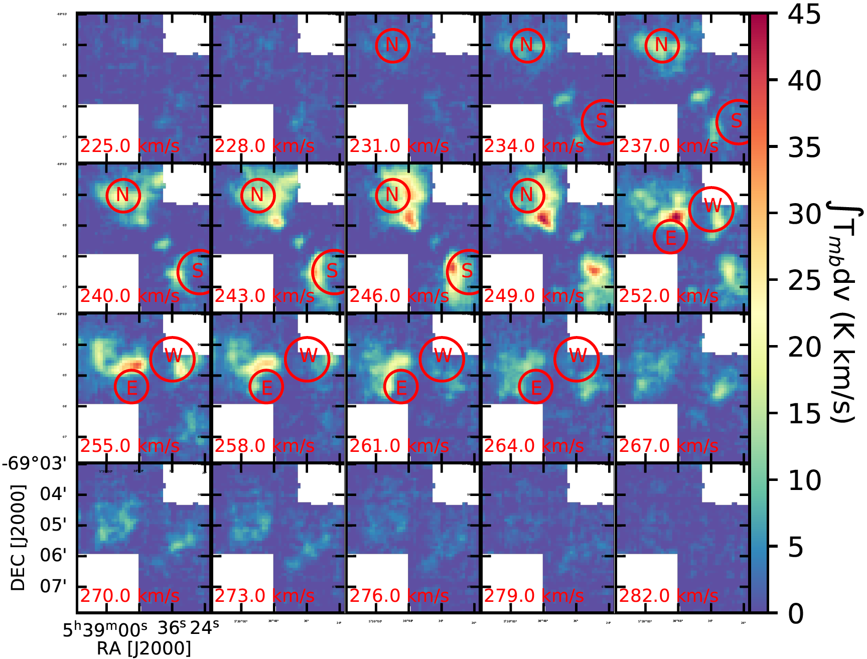
Figure 15: Channel maps of the 30 Dor region, in steps of 3 km s^-1, displaying the [CII] dynamics of the region. The red circles indicate the expanding shell candidates from Table 1 in their proposed velocity with their name.

Appendix B Magnetic fields using CO(2-1)

Figure 16, left panel shows maps of the strength of B-field estimated using the velocity dispersion from CO(2-1). A similar structure as in Figure 10 is seen but the amplitude is slightly lower because of the narrower velocity dispersion of CO(2-1) (see lower panels in Figure 5). Right panels of Figure 16 and Figure 17 show the mass-to-flux ratio, Afvénic Mach number and turbulence-to-magnetic pressure ratio. As seen in [CII], magnetic field is sufficient strong to take over the gravitational potential and turbulence pressure except at the peak intensity.

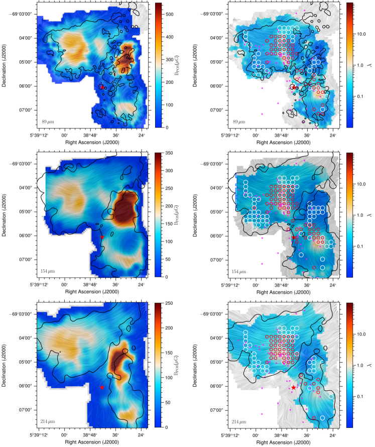
Figure 16: Left: Magnetic field strength estimated by DCF method similar using CO(2-1) data. Right: Mass-to-flux ratio derived by the field strength on the left panel. Symbols are the same as in Figure 11.

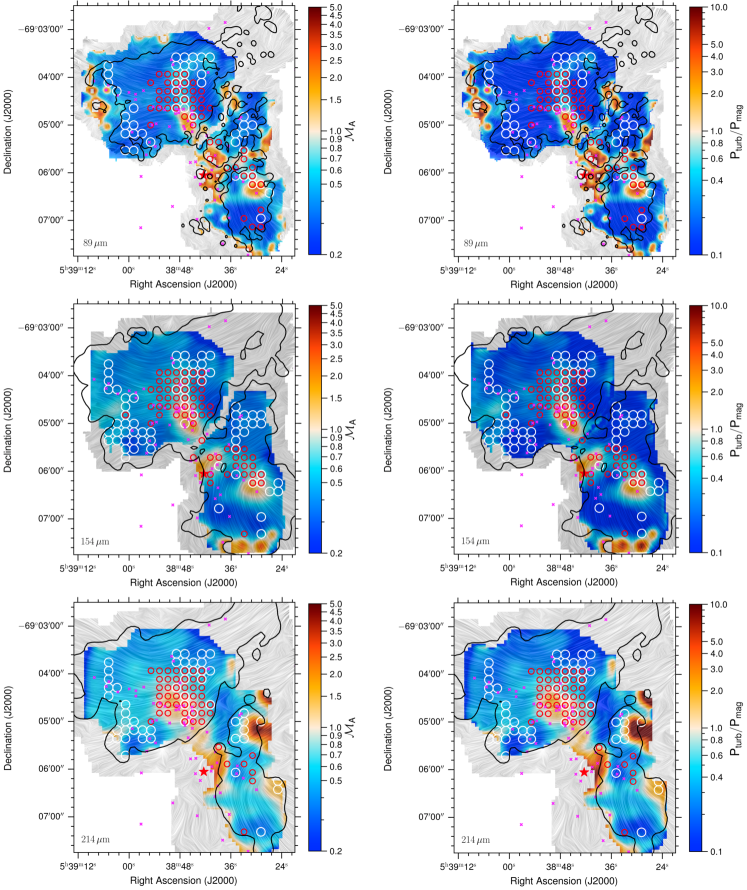
Figure 17: Afvénic Mach number (left panel) and turbulent-to-magnetic pressure ratio (right panel) derived by the field strength in Figure 16. Symbols are the same as in Figure 11.

References

- Abe et al. (2021) Abe, D., Inoue, T., Inutsuka, S.-i., & Matsumoto, T. 2021, ApJ, 916, 83, doi: 10.3847/1538-4357/ac07a1
- Alina et al. (2022) Alina, D., Montillaud, J., Hu, Y., et al. 2022, A&A, 658, A90, doi: 10.1051/0004-6361/202039065
- Andersson et al. (2015) Andersson, B. G., Lazarian, A., & Vaillancourt, J. E. 2015, ARA& A, 53, 501, doi: 10.1146/annurev-astro-082214-122414
- Arthur et al. (2011) Arthur, S. J., Henney, W. J., Mellema, G., de Colle, F., & Vázquez-Semadeni, E. 2011, MNRAS, 414, 1747, doi: 10.1111/j.1365-2966.2011.18507.x
- Beuther et al. (2022) Beuther, H., Schneider, N., Simon, R., et al. 2022, A&A, 659, A77. doi:10.1051/0004-6361/202142689
- Bonne et al. (2020a) Bonne, L., Schneider, N., Bontemps, S., et al. 2020a, A&A, 641, A17, doi: 10.1051/0004-6361/201937104
- Bonne et al. (2020b) Bonne, L., Bontemps, S., Schneider, N., et al. 2020b, A&A, 644, A27, doi: 10.1051/0004-6361/202038281
- Bonne et al. (2022a) Bonne, L., Schneider, N., García, P., et al. 2022, ApJ, 935, 171. doi:10.3847/1538-4357/ac8052
- Bonne et al. (2022b) Bonne, L., Peretto, N., Duarte-Cabral, A., et al. 2022, arXiv:2206.10889
- Brandl (2005) Brandl, B. R. 2005, in Astrophysics and Space Science Library, Vol. 329, Starbursts: From 30 Doradus to Lyman Break Galaxies, ed. R. de Grijs & R. M. González Delgado, 49, doi: 10.1007/1-4020-3539-X_10
- Cabral & Leedom (1993) Cabral, B., & Leedom, L. C. 1993, in Proceedings of the 20th Annual Conference on Computer Graphics and Interactive Techniques, SIGGRAPH ’93 (New York, NY, USA: Association for Computing Machinery), 263–270, doi: 10.1145/166117.166151
- Chandrasekhar & Fermi (1953) Chandrasekhar, S., & Fermi, E. 1953, ApJ, 118, 113, doi: 10.1086/145731
- Chen et al. (2019) Chen, C.-Y., King, P. K., Li, Z.-Y., Fissel, L. M., & Mazzei, R. R. 2019, MNRAS, 485, 3499, doi: 10.1093/mnras/stz618
- Chevance et al. (2020) Chevance, M., Madden, S. C., Fischer, C., et al. 2020, MNRAS, 494, 5279, doi: 10.1093/mnras/staa1106
- Cho & Lazarian (2003) Cho, J., & Lazarian, A. 2003, MNRAS, 345, 325, doi: 10.1046/j.1365-8711.2003.06941.x
- Chu & Kennicutt (1994) Chu, Y.-H., & Kennicutt, Robert C., J. 1994, ApJ, 425, 720, doi: 10.1086/174017
- Crutcher (2012) Crutcher, R. M. 2012, ARA& A, 50, 29, doi: 10.1146/annurev-astro-081811-125514
- Crutcher et al. (2004) Crutcher, R. M., Nutter, D. J., Ward-Thompson, D., & Kirk, J. M. 2004, ApJ, 600, 279, doi: 10.1086/379705
- Davis (1951) Davis, L. 1951, Physical Review, 81, 890, doi: 10.1103/PhysRev.81.890.2
- Devaraj et al. (2021) Devaraj, R., Clemens, D. P., Dewangan, L. K., et al. 2021, ApJ, 911, 81, doi: 10.3847/1538-4357/abe9b1
- Dolginov & Mytrophanov (1976) Dolginov, A. Z., & Mytrophanov, I. G. 1976, Ap&SS, 43, 257, doi: 10.1007/BF00640009
- Eswaraiah et al. (2021) Eswaraiah, C., Li, D., Furuya, R. S., et al. 2021, ApJL, 912, L27, doi: 10.3847/2041-8213/abeb1c
- Ewertowski & Basu (2013) Ewertowski, B., & Basu, S. 2013, ApJ, 767, 33, doi: 10.1088/0004-637X/767/1/33
- Federrath & Klessen (2013) Federrath, C., & Klessen, R. S. 2013, ApJ, 763, 51, doi: 10.1088/0004-637X/763/1/51
- Federrath et al. (2010) Federrath, C., Roman-Duval, J., Klessen, R. S., Schmidt, W., & Mac Low, M. M. 2010, A&A, 512, A81, doi: 10.1051/0004-6361/200912437
- Girichidis et al. (2014) Girichidis, P., Konstandin, L., Whitworth, A. P., & Klessen, R. S. 2014, ApJ, 781, 91, doi: 10.1088/0004-637X/781/2/91
- González-Casanova & Lazarian (2017) González-Casanova, D. F., & Lazarian, A. 2017, ApJ, 835, 41, doi: 10.3847/1538-4357/835/1/41
- Gordon et al. (2018) Gordon, M. S., Lopez-Rodriguez, E., Andersson, B. G., et al. 2018, arXiv e-prints, arXiv:1811.03100. https://arxiv.org/abs/1811.03100
- Guerra et al. (2021) Guerra, J. A., Chuss, D. T., Dowell, C. D., et al. 2021, ApJ, 908, 98, doi: 10.3847/1538-4357/abd6f0
- Güsten et al. (2006) Güsten, R., Nyman, L. Å., Schilke, P., et al. 2006, A&A, 454, L13, doi: 10.1051/0004-6361:20065420
- Hacar et al. (2016) Hacar, A., Alves, J., Burkert, A., & Goldsmith, P. 2016, A&A, 591, A104, doi: 10.1051/0004-6361/201527319
- Hartmann & Burkert (2007) Hartmann, L., & Burkert, A. 2007, ApJ, 654, 988, doi: 10.1086/509321
- Henney et al. (2009) Henney, W. J., Arthur, S. J., de Colle, F., & Mellema, G. 2009, MNRAS, 398, 157, doi: 10.1111/j.1365-2966.2009.15153.x
- Hoang et al. (2022) Hoang, T., Tram, L. N., Phan, V. H. M., et al. 2022, arXiv:2205.02334
- Hoang et al. (2021b) Hoang, T. D., Bich Ngoc, N., Diep, P. N., et al. 2021b, arXiv e-prints, arXiv:2108.10045. https://arxiv.org/abs/2108.10045
- Houde et al. (2009) Houde, M., Vaillancourt, J. E., Hildebrand, R. H., Chitsazzadeh, S., & Kirby, L. 2009, ApJ, 706, 1504, doi: 10.1088/0004-637X/706/2/1504
- Hu et al. (2021a) Hu, Y., Lazarian, A., & Stanimirović, S. 2021a, ApJ, 912, 2, doi: 10.3847/1538-4357/abedb7
- Hu et al. (2021b) Hu, Y., Lazarian, A., & Wang, Q. D. 2021b, arXiv e-prints, arXiv:2105.03605. https://arxiv.org/abs/2105.03605
- Hu et al. (2018) Hu, Y., Yuen, K. H., & Lazarian, A. 2018, MNRAS, 480, 1333, doi: 10.1093/mnras/sty1807
- Hu et al. (2019a) Hu, Y., Yuen, K. H., & Lazarian, A. 2019a, ApJ, 886, 17, doi: 10.3847/1538-4357/ab4b5e
- Hu et al. (2019b) Hu, Y., Yuen, K. H., Lazarian, V., et al. 2019b, Nature Astronomy, 3, 776, doi: 10.1038/s41550-019-0769-0
- Indebetouw et al. (2009) Indebetouw, R., de Messières, G. E., Madden, S., et al. 2009, ApJ, 694, 84, doi: 10.1088/0004-637X/694/1/84
- Indebetouw et al. (2013) Indebetouw, R., Brogan, C., Chen, C. H. R., et al. 2013, ApJ, 774, 73, doi: 10.1088/0004-637X/774/1/73
- Inoue & Fukui (2013) Inoue, T., & Fukui, Y. 2013, ApJL, 774, L31, doi: 10.1088/2041-8205/774/2/L31
- Jackson et al. (2019) Jackson, J. M., Whitaker, J. S., Rathborne, J. M., et al. 2019, ApJ, 870, 5, doi: 10.3847/1538-4357/aaef84
- Kainulainen et al. (2014) Kainulainen, J., Federrath, C., & Henning, T. 2014, Science, 344, 183, doi: 10.1126/science.1248724
- Kandori et al. (2020) Kandori, R., Tamura, M., Saito, M., et al. 2020, ApJ, 892, 128, doi: 10.3847/1538-4357/ab7b68
- Kennicutt (1984) Kennicutt, R. C., J. 1984, ApJ, 287, 116, doi: 10.1086/162669
- Kim et al. (2016) Kim, J., Jeong, W.-S., Pak, S., Park, W.-K., & Tamura, M. 2016, ApJS, 222, 2, doi: 10.3847/0067-0049/222/1/2
- Kim et al. (1999) Kim, S., Dopita, M. A., Staveley-Smith, L., & Bessell, M. S. 1999, AJ, 118, 2797, doi: 10.1086/301116
- Klein et al. (1993) Klein, U., Haynes, R. F., Wielebinski, R., & Meinert, D. 1993, A&A, 271, 402
- Klessen (2000) Klessen, R. S. 2000, ApJ, 535, 869, doi: 10.1086/308854
- Körtgen et al. (2019) Körtgen, B., Federrath, C., & Banerjee, R. 2019, MNRAS, 482, 5233, doi: 10.1093/mnras/sty3071
- Lazarian (2007) Lazarian, A. 2007, J. Quant. Spec. Radiat. Transf., 106, 225, doi: 10.1016/j.jqsrt.2007.01.038
- Lazarian (2014) Lazarian, A. 2014, Space Sci. Rev., 181, 1, doi: 10.1007/s11214-013-0031-5
- Lazarian & Pogosyan (2000) Lazarian, A., & Pogosyan, D. 2000, ApJ, 537, 720, doi: 10.1086/309040
- Lazarian & Vishniac (1999) Lazarian, A., & Vishniac, E. T. 1999, ApJ, 517, 700, doi: 10.1086/307233
- Lazarian & Yuen (2018) Lazarian, A., & Yuen, K. H. 2018, ApJ, 853, 96, doi: 10.3847/1538-4357/aaa241
- Lazarian et al. (2018) Lazarian, A., Yuen, K. H., Ho, K. W., et al. 2018, ApJ, 865, 46, doi: 10.3847/1538-4357/aad7ff
- Lazarian et al. (2020) Lazarian, A., Yuen, K. H., & Pogosyan, D. 2020, arXiv e-prints, arXiv:2002.07996. https://arxiv.org/abs/2002.07996
- Lazarian et al. (2022) —. 2022, ApJ, 935, 77, doi: 10.3847/1538-4357/ac6877
- Schneider et al. (2018) Schneider, N., Röllig, M., Simon, R., et al. 2018, A&A, 617, A45. doi:10.1051/0004-6361/201732508
- Lee et al. (2019) Lee, M. Y., Madden, S. C., Le Petit, F., et al. 2019, A&A, 628, A113, doi: 10.1051/0004-6361/201935215
- Li et al. (2022) Li, P. S., Lopez-Rodriguez, E., Ajeddig, H., et al. 2022, MNRAS, 510, 6085, doi: 10.1093/mnras/stab3448
- Liu et al. (2022) Liu, J., Qiu, K., & Zhang, Q. 2022, ApJ, 925, 30, doi: 10.3847/1538-4357/ac3911
- Lopez et al. (2011) Lopez, L. A., Krumholz, M. R., Bolatto, A. D., Prochaska, J. X., & Ramirez-Ruiz, E. 2011, ApJ, 731, 91, doi: 10.1088/0004-637X/731/2/91
- Lu et al. (2020) Lu, Z., Lazarian, A., & Pogosyan, D. 2020, MNRAS, 496, 2868, doi: 10.1093/mnras/staa1570
- Luisi et al. (2021) Luisi, M., Anderson, L. D., Schneider, N., et al. 2021, Science Advances, 7, eabe9511, doi: 10.1126/sciadv.abe9511
- Mac Low & Klessen (2004) Mac Low, M.-M., & Klessen, R. S. 2004, Reviews of Modern Physics, 76, 125, doi: 10.1103/RevModPhys.76.125
- Mackey & Lim (2011) Mackey, J., & Lim, A. J. 2011, MNRAS, 412, 2079, doi: 10.1111/j.1365-2966.2010.18043.x
- Mao et al. (2012) Mao, S. A., McClure-Griffiths, N. M., Gaensler, B. M., et al. 2012, ApJ, 759, 25, doi: 10.1088/0004-637X/759/1/25
- Meixner et al. (2013) Meixner, M., Panuzzo, P., Roman-Duval, J., et al. 2013, AJ, 146, 62, doi: 10.1088/0004-6256/146/3/62
- Melnick et al. (2021) Melnick, J., Tenorio-Tagle, G., & Telles, E. 2021, A&A, 649, A175, doi: 10.1051/0004-6361/201937268
- Mestel (1966) Mestel, L. 1966, MNRAS, 133, 265, doi: 10.1093/mnras/133.2.265
- Nakajima et al. (2007) Nakajima, Y., Kandori, R., Tamura, M., et al. 2007, PASJ, 59, 519, doi: 10.1093/pasj/59.3.519
- Ngoc et al. (2021) Ngoc, N. B., Diep, P. N., Parsons, H., et al. 2021, ApJ, 908, 10, doi: 10.3847/1538-4357/abd0fc
- Okada et al. (2019) Okada, Y., Güsten, R., Requena-Torres, M. A., et al. 2019, A&A, 621, A62, doi: 10.1051/0004-6361/201833398
- Pabst et al. (2019) Pabst, C., Higgins, R., Goicoechea, J. R., et al. 2019, Nature, 565, 618, doi: 10.1038/s41586-018-0844-1
- Pabst et al. (2020) Pabst, C. H. M., Goicoechea, J. R., Teyssier, D., et al. 2020, A&A, 639, A2, doi: 10.1051/0004-6361/202037560
- Pattle et al. (2018) Pattle, K., Ward-Thompson, D., Hasegawa, T., et al. 2018, ApJL, 860, L6, doi: 10.3847/2041-8213/aac771
- Pellegrini et al. (2011) Pellegrini, E. W., Baldwin, J. A., & Ferland, G. J. 2011, ApJ, 738, 34, doi: 10.1088/0004-637X/738/1/34
- Peretto et al. (2006) Peretto, N., André, P., & Belloche, A. 2006, A&A, 445, 979, doi: 10.1051/0004-6361:20053324
- Peretto et al. (2013) Peretto, N., Fuller, G. A., Duarte-Cabral, A., et al. 2013, A&A, 555, A112, doi: 10.1051/0004-6361/201321318
- Phillips et al. (1979) Phillips, T. G., Huggins, P. J., Wannier, P. G., & Scoville, N. Z. 1979, ApJ, 231, 720, doi: 10.1086/157237
- Pineda et al. (2008) Pineda, J. E., Caselli, P., & Goodman, A. A. 2008, ApJ, 679, 481, doi: 10.1086/586883
- Schneider et al. (2020) Schneider, N., Simon, R., Guevara, C., et al. 2020, PASP, 132, 104301. doi:10.1088/1538-3873/aba840
- Santos et al. (2019) Santos, F. P., Chuss, D. T., Dowell, C. D., et al. 2019, ApJ, 882, 113, doi: 10.3847/1538-4357/ab3407
- Schaefer (2008) Schaefer, B. E. 2008, AJ, 135, 112, doi: 10.1088/0004-6256/135/1/112
- Schneider et al. (2010) Schneider, N., Csengeri, T., Bontemps, S., et al. 2010, A&A, 520, A49, doi: 10.1051/0004-6361/201014481
- Schneider et al. (2013) Schneider, N., André, P., Könyves, V., et al. 2013, ApJL, 766, L17, doi: 10.1088/2041-8205/766/2/L17
- Schneider et al. (2015) Schneider, N., Bontemps, S., Girichidis, P., et al. 2015, MNRAS, 453, L41, doi: 10.1093/mnrasl/slv101
- Schneider et al. (2022) Schneider, N., Ossenkopf-Okada, V., Clarke, S., et al. 2022, arXiv:2207.14604
- Skalidis et al. (2021a) Skalidis, R., Sternberg, J., Beattie, J. R., Pavlidou, V., & Tassis, K. 2021a, A&A, 656, A118, doi: 10.1051/0004-6361/202142045
- Skalidis & Tassis (2021) Skalidis, R., & Tassis, K. 2021, A&A, 647, A186, doi: 10.1051/0004-6361/202039779
- Skalidis et al. (2021b) Skalidis, R., Tassis, K., Panopoulou, G. V., et al. 2021, arXiv e-prints, arXiv:2110.11878. https://arxiv.org/abs/2110.11878
- Soam et al. (2018a) Soam, A., Maheswar, G., Lee, C. W., Neha, S., & Kim, K.-T. 2018a, MNRAS, 476, 4782, doi: 10.1093/mnras/sty517
- Soam et al. (2018b) Soam, A., Pattle, K., Ward-Thompson, D., et al. 2018b, ApJ, 861, 65, doi: 10.3847/1538-4357/aac4a6
- Tahani et al. (2019) Tahani, M., Plume, R., Brown, J. C., Soler, J. D., & Kainulainen, J. 2019, A&A, 632, A68, doi: 10.1051/0004-6361/201936280
- Tang et al. (2019) Tang, Y.-W., Koch, P. M., Peretto, N., et al. 2019, ApJ, 878, 10, doi: 10.3847/1538-4357/ab1484
- Tiwari et al. (2021) Tiwari, M., Karim, R., Pound, M. W., et al. 2021, ApJ, 914, 117, doi: 10.3847/1538-4357/abf6ce
- Townsley et al. (2006) Townsley, L. K., Broos, P. S., Feigelson, E. D., et al. 2006, AJ, 131, 2140, doi: 10.1086/500532
- Tram & Hoang (2022) Tram, L. N. & Hoang, T. 2022, arXiv:2208.13195
- Tram et al. (2021c) Tram, L. N., Hoang, T., Lopez-Rodriguez, E., et al. 2021c, arXiv e-prints, arXiv:2105.09530. https://arxiv.org/abs/2105.09530
- Young et al. (2012) Young, E. T., Becklin, E. E., Marcum, P. M., et al. 2012, ApJL, 749, L17, doi: 10.1088/2041-8205/749/2/L17
- Yuen & Lazarian (2017a) Yuen, K. H., & Lazarian, A. 2017a, ApJL, 837, L24, doi: 10.3847/2041-8213/aa6255
- Yuen & Lazarian (2017b) —. 2017b, arXiv e-prints, arXiv:1703.03026. https://arxiv.org/abs/1703.03026