Robust tests for equality of regression curves
based on characteristic functions

Abstract

This paper focuses on the problem of testing the null hypothesis that the regression functions of several populations are equal under a general nonparametric homoscedastic regression model. It is well known that linear kernel regression estimators are sensitive to atypical responses. These distorted estimates will influence the test statistic constructed from them so the conclusions obtained when testing equality of several regression functions may also be affected. In recent years, the use of testing procedures based on empirical characteristic functions has shown good practical properties. For that reason, to provide more reliable inferences, we construct a test statistic that combines characteristic functions and residuals obtained from a robust smoother under the null hypothesis. The asymptotic distribution of the test statistic is studied under the null hypothesis and under root$-n$ contiguous alternatives. A Monte Carlo study is performed to compare the finite sample behaviour of the proposed test with the classical one obtained using local averages. The reported numerical experiments show the advantage of the proposed methodology over the one based on Nadaraya–Watson estimators for finite samples. An illustration to a real data set is also provided and enables to investigate the sensitivity of the $p-$value to the bandwidth selection.

Key Words: Hypothesis testing, Nonparametric regression models, Robust estimation, Smoothing techniques.

1 Introduction

Let us assume that the random vectors $(X_{j},Y_{j})^{\mbox{\footnotesize\sc t}}$, $j=1,\dots,k$, follow the homoscedastic nonparametric regression models

$$Y_{j}=m_{j}(X_{j})+U_{j}=m_{j}(X_{j})+\sigma_{j}\varepsilon_{j},$$ (1)

where $m_{j}:\mathbb{R}\to\mathbb{R}$ is a nonparametric smooth function and the error $\varepsilon_{j}$ is independent of the covariate $X_{j}$. The nonparametric nature of model (1) offers more flexibility than the standard linear model when modelling a complicated relationship between the response variable and the covariate. As is usual in a robust framework, we will avoid first moment conditions and we will require that the errors distribution $G_{j}(\cdot)$ has scale $1$. Furthermore, to identify $m_{j}$ we will impose an identifiability assumption depending on the score function (see assumption A3 below) which holds whenever the errors $\varepsilon_{j}$ have a symmetric distribution. For instance, if the target, that is, the quantity of interest, is the conditional median, the loss function to be used should be the absolute value. In such a situation, to identify $m_{j}$, the requirement is that the error $\varepsilon_{j}$ has median $0$. When second moments exist, as it is the case of the classical approach, the usual assumption is that $\mathbb{E}(\varepsilon_{j})=0$ and $\mbox{\sc Var}(\varepsilon_{j})=1$, which means that $m_{j}$ represents the conditional mean, while $\sigma_{j}^{2}$ equals the residuals variance, i.e., $\sigma_{j}^{2}=\mbox{\sc Var}(Y_{j}-m_{j}(X_{j}))$. Henceforth, we assume that the covariates $X_{j}$ have the same support ${\mathcal{R}}$, even when they may have different densities.

In many situations, it is of interest to compare the regression functions $m_{j}$, $j=1,\dots,k$, to decide if the same functional form appears in all populations. In particular, in this paper we focus on testing the null hypothesis of equality of the regression curves at least in some region ${\mathcal{R}}_{0}$ of the common support ${\mathcal{R}}$, versus a general alternative. The null hypothesis to be considered is

$$H_{0}:m_{1}(x)=m_{2}(x)=\dots=m_{k}(x)\text{ for all }x\in{\mathcal{R}}_{0},$$ (2)

while the alternative hypothesis is $H_{1}:H_{0}\mbox{ is not true}$.

When second moments exist, the problem of testing equality of two regression curves has been considered by several authors such as Dette and Munk, (1998) and Neumeyer and Dette, (2003), among others. The first paper considered almost uniform design points and construct an $L^{2}$ statistic for which the asymptotic distribution is derived under the null hypothesis and under fixed alternatives, while the second one proposed and studied a procedure based on the comparison of marked empirical processes of the residuals. Some possible extensions to the situation of $k>2$ were already mentioned therein. As mentioned in Pardo-Fernández et al., (2007), the extension of the test statistics used when comparing two regression curves to the situation of $k>2$ regression functions may not be straightforward, since some loss of power may arise when performing comparisons pairwise. To solve this issue, Pardo-Fernández et al., (2007) proposed Kolmogorov–Smirnov and Cramér–von Mises type statistics and establish their asymptotic distribution under the null hypothesis and under root-$n$ local alternatives. These statistics were constructed using the empirical distribution functions of the residuals obtained from non-parametric kernel estimators. Pardo-Fernández et al., (2015) introduced a statistic based on the residuals characteristic functions which can detect local alternatives converging to the null hypothesis at the rate $\sqrt{n}$ and whose $p-$values do not rely on bootstrap. In this paper, we will provide a robust alternative to this procedure.

The main reason to provide a robust counterpart is that the test statistic based on characteristic functions mentioned above is based on linear kernel regression estimators which locally average the responses resulting in estimators sensitive to atypical observations. More precisely, when estimating the regression function at a value $x$, the effect of an outlier in the responses will be larger as the distance between the related covariate and the point $x$ is smaller. In this sense, atypical data in the responses in nonparametric regression may lead to a complete distorted estimation which will clearly influence the test statistic and the conclusions of the testing procedure. Hence, robust estimates are needed to provide more reliable estimations and inferences. Beyond the importance of developing robust estimators, the problem of obtaining robust hypothesis testing procedures also deserves attention. In the nonparametric setting, robust testing procedures are scarce. For instance, a robust test for homoscedasticity in nonparametric regression was defined in Dette and Marchlewski, (2010), while Bianco et al., (2006) proposed a procedure to test if the nonparametric component equals a fixed given function in the framework of a partly linear regression model. On the other hand, Sun, (2006) proposed a test based on an orthogonal moment condition of residuals which converges at non–parametric rate, while Dette et al., (2011, 2013) provided a test based on the $L^{2}-$distance between non-crossing non-parametric estimates of the quantile curves, the first one converges at the non–parametric rate $\sqrt{nh}$, where $h$ is the bandwidth parameter, while the latter one detects alternatives at rate root-$n$. Finally, the proposal in Kuruwita et al., (2014) is based on a marked empirical process of the residuals detecting also root-$n$ alternatives. A robust approach to compare two regression functions versus a one-sided alternative, using local $M-$estimators, was studied in Boente and Pardo-Fernández, (2016). Their proposal is based on a test statistic that uses a bounded score function and the residuals obtained from a robust estimate for the regression function under the null hypothesis. When the errors in both populations have the same distribution and the design points have equal densities, Koul and Schick, (1997) defined a family of covariate–matched statistics allowing to detect root$-n$ one–sided local alternatives. It is worth mentioning that this family includes a covariate–matched Wilcoxon–Mann–Whitney test based on the sign of all response differences, for which the asymptotic properties are derived without requiring second moments to the errors. To extend their proposal to the situation of different errors distribution and possible different error densities, Koul and Schick, (2003) developed a modified version of one of the covariate–matched statistics introduced in Koul and Schick, (1997), but this statistic assumes the existence of second moments and may be affected by atypical data arise in the responses. Finally, Feng et al., (2015) considered a test for $H_{0}$ versus $H_{1}$ using a generalized likelihood ratio test incorporating a Wilcoxon likelihood function and kernel smoothers, which allows to detect alternatives with non–parametric rate. In order to obtain asymptotic results for their proposal Feng et al., (2015) assumed that the errors $\varepsilon_{j}$ have symmetric distributions with Lipschitz densities as well as the existence of second moment of the regression errors.

The aim of this paper is to propose a class of tests for $H_{0}$ versus $H_{1}$ in (2) which combines the ideas of robust smoothing with those given in Pardo-Fernández et al., (2015) to obtain a procedure detecting root$-n$ alternatives without requiring first moments to the errors. In Section 2, we remind the definition of the robust estimators. The test statistics is introduced in Section 3, where its asymptotic behaviour under the null hypothesis and contiguous alternatives is also studied. We present the results of a Monte Carlo study in Section 4 and an illustration to a real data set in Section 5. Final comments are provided in Section 6. All proofs are relegated to the Appendix.

2 Preliminaries on robust regression estimation

As mentioned above, the robust statistic to be defined is based on robust local $M-$smoothers. For that reason, in this section, we briefly review their definition and state the notation to be employed.

Let $(X_{j\ell},Y_{j\ell})^{\mbox{\footnotesize\sc t}}$, $1\leq i\leq n_{j}$, be independent and identically distributed observations with the same distribution as $(X_{j},Y_{j})^{\mbox{\footnotesize\sc t}}$, $j=1,\ldots,k$. As it is well known, if $\mathbb{E}|Y_{j}|<\infty$, the regression functions $m_{j}$ in (1) equals $\mathbb{E}(Y_{j}|X_{j})$, which may be estimated using the Nadaraya–Watson estimator (see, for example, Härdle, , 1990). To remind its definition, let $K$ be a kernel function (usually a symmetric density) and $h=h_{n}$ a sequence of strictly positive real numbers. Furthermore, let $K_{h}(u)=h^{-1}K(u/h)$. The linear kernel smoother used to estimate $m_{j}$ is defined as

$$\widehat{m}_{j,\mbox{\footnotesize\sc cl}}(x)=\left\{\sum_{\ell=1}^{n_{j}}K_{h}\left(x-X_{j\ell}\right)\right\}^{-1}\sum_{\ell=1}^{n_{j}}K_{h}\left(x-X_{j\ell}\right)Y_{j\ell}\,.$$ (3)

As mentioned in the introduction, this estimator is sensitive to outlying values in the response variable, also known as “vertical outliers” in the literature. Robust estimates in a nonparametric setting provide an alternative to obtain estimators insensitive to atypical data. Among the proposals considered in the literature, we can mention the local $M-$smoothers studied in Härdle and Tsybakov, (1988) and Boente and Fraiman, (1989), among others. These estimators use a preliminary scale estimator to measure the size of the residuals to be downweighted. For heteroscedastic models, the scale function can only be estimated at a nonparametric rate. In contrast, under an homoscedastic regression model, root$-n$ scale estimators may be constructed. In particular, scale estimators based on differences are widely used, see, for instance, Rice, (1984) and Hall et al., (1990). Ghement et al., (2008) proposed a robust version of these difference–based estimators. For random covariates, let $X_{j,(1)}\leq\dots\leq X_{j,(n_{j})}$ be the ordered statistics of the explanatory variables of the $j-$th population and denote as $(X_{j,(1)},Y_{j,D_{1,j}})^{\mbox{\footnotesize\sc t}},\dots,(X_{j,(n_{j})},Y_{j,D_{n_{j},j}})^{\mbox{\footnotesize\sc t}}$ the sample of observations ordered according to the values of the explanatory variables, that is, $X_{j,(\ell)}=X_{j,D_{\ell,j}}$. The estimators defined in Ghement et al., (2008) can be adapted to the present situation by taking the differences $Y_{j,D_{\ell+1,j}}-Y_{j,D_{\ell,j}}$, see also Dette and Munk, (1998). From these differences, one may define the robust consistent root$-n$ scale estimator of $\sigma_{j}$ as

$$\widehat{\sigma}_{j}=\frac{1}{\sqrt{2}\Phi^{-1}(3/4)}\mathop{\mbox{median}}_{1\leq\ell\leq n_{j}-1}\left|Y_{j,D_{\ell+1,j}}-Y_{j,D_{\ell,j}}\right|,$$ (4)

where the coefficient $\sqrt{2}\Phi^{-1}(3/4)$ ensures Fisher-consistency for normal errors ($\Phi^{-1}$ denotes the quantile function of the standard normal law).

Let $\rho_{j}:\mathbb{R}\to\mathbb{R}$, $j=1,\ldots,k$, be a $\rho-$function as defined in Maronna et al., (2019), that is, a continuous and even function non-decreasing on $[0,+\infty)$ and such that $\rho_{j}(0)=0$. Moreover, $\lim_{u\to\infty}\rho_{j}(u)\neq 0$ and if $0\leq u<v$ with $\rho_{j}(v)<\sup_{u}\rho_{j}(u)$ then $\rho_{j}(u)<\rho_{j}(v)$. When $\rho_{j}$ is bounded, we assume that $\sup_{u}\rho_{j}(u)=1$. If $\rho_{j}$ is differentiable, we denote as $\psi_{j}$ its derivative. It is often required that $\psi_{j}$ is bounded, as happens in the following examples. Two widely used families of $\rho-$functions are the Huber’s function and the Tukey’s bisquare one. In both cases, $\rho_{j}(u)=\rho_{0}(u/c_{j})$, where $c_{j}>0$ is a tuning constant to achieve a given efficiency. The $\rho-$function $\rho_{0}$ related to the proposal in Huber, (1964) was extensively used in regression problems with fixed covariates and corresponds to $\rho_{0}(u)=\rho_{\mbox{\scriptsize\sc h}}(u)\,=\,u^{2}/2$ when $|u|\leq 1$, while $\rho_{\mbox{\scriptsize\sc h}}\left(u\right)=|u|-1/2$, otherwise. It leads to an unbounded $\rho-$function with bounded derivative $\psi_{\mbox{\scriptsize\sc h}}(u)=\min\{1,\max(-1,u)\}$. A a smooth approximation of the Huber function defined as $\rho_{0}(u)=\sqrt{1+u^{2}}-1$ may also be considered. The Tukey’s bisquare function corresponds to a bounded $\rho-$function and is defined as $\rho_{0}(u)=\rho_{\,\mbox{\scriptsize\sc t}}(u)=\min\left\{1-(1-u^{2})^{3},1\right\}$. It is worth mentioning that the bounded derivative of the $\rho-$function controls the effect of “vertical outliers”. Clearly, different tuning constants or $\rho-$functions may be chosen when defining $\rho_{j}$ for each $j=1,\dots,k$, even when it is preferable to ensure the same efficiency in the estimation procedure across populations.

Define

$$\lambda_{j}(x,a,\sigma)=\mathbb{E}\left[\psi_{j}\left(\frac{Y_{j}-a}{\sigma}\right)|X_{j}=x\right]\mbox{ and }\gamma_{j}(x,a,\sigma)=\mathbb{E}\left[\rho_{j}\left(\frac{Y_{j}-a}{\sigma}\right)|X_{j}=x\right].$$ (5)

Note that if (1) holds, $\psi_{j}$ is an odd function and the errors have a symmetric distribution, then $\lambda_{j}(x,m_{j}(x),\sigma)=\mathbb{E}\psi_{j}(\sigma_{j}\varepsilon_{j}/\sigma)=0$, for any $\sigma>0$. Moreover, taking into account that the errors are independent of the covariates, we have that

$$\gamma_{j}(x,a,\sigma)=\mathbb{E}\left[\rho_{j}\left(\frac{\sigma_{j}\,\varepsilon_{j}+m_{j}(x)-a}{\sigma}\right)\right]\,.$$

Therefore, Lemma 3.1 in Yohai, (1985) (see also Maronna et al., , 2019, Theorem 10.2) entails that $m_{j}(x)$ is the unique minimizer of $\gamma_{j}(x,a,\sigma)$ when $\rho_{j}$ is a $\rho-$function, the errors $\varepsilon_{j}$ have a density function $g_{j}(t)$ that is even, non-increasing in $|t|$, and strictly decreasing for $|t|$ in a neighbourhood of $0$ .

Hence, to obtain robust estimators of $m_{j}(x)$, we plug into (5) an estimator of the conditional distribution of $Y_{j}|X_{j}=x$ and a robust estimator of the error’s scale $\widehat{\sigma}_{j}$, such as the one defined in (4). Based on the samples $\{(X_{j\ell},Y_{j\ell})^{\mbox{\footnotesize\sc t}},\ell=1,\ldots,n_{j}\}$, the robust nonparametric estimator of $m_{j}(x)$ is defined as the minimizer $\widehat{m}_{j}(x)$ of $\widehat{\gamma}_{j}(x,a,\widehat{\sigma}_{j})$, where

$$\widehat{\gamma}_{j}(x,a,\sigma)=\sum_{\ell=1}^{n_{j}}K_{h}\left(x-X_{j\ell}\right)\rho_{j}\left(\frac{Y_{j\ell}-a}{\sigma}\right)\,.$$ (6)

Hence, $\widehat{m}_{j}(x)$ is the solution of

$$\widehat{\lambda}_{j}(x,\widehat{m}_{j}(x),\widehat{\sigma}_{j})=0\,,$$ (7)

with

$$\widehat{\lambda}_{j}(x,a,\sigma)=\sum_{\ell=1}^{n_{j}}K_{h}\left(x-X_{j\ell}\right)\psi_{j}\left(\frac{Y_{j\ell}-a}{\sigma}\right)\,,$$ (8)

Note that different $\rho-$functions $\rho_{j}$ can be used in the different samples, in this way, we provide a more flexible setting.

3 A class of test statistics

As in Hus̆ková and Meintanis, (2009) and Pardo-Fernández et al., (2015), our test will be based on a weighted $L^{2}-$distance between characteristic functions. We will compare the characteristic functions of the residuals obtained from a robust fit with those constructed under the null hypothesis. For that purpose, let $m_{0}$ be the common regression curve under the null hypothesis and define

$$\varepsilon_{0j}=\frac{Y_{j}-m_{0}(X_{j})}{\sigma_{j}}\,.$$

It turns out that the null hypothesis $H_{0}$ is true if and only if, for all $1\leq j\leq k$, the random variables $\varepsilon_{j}$ and $\varepsilon_{0j}$ have the same distribution for some function $m_{0}$, see Pardo-Fernández et al., (2007).

Let $W_{j}:\mathbb{R}\to\mathbb{R}$ be a non-negative weight function with compact support ${\mathcal{S}}_{j}\subset\accentset{\circ}{{\mathcal{R}}}$, where $\accentset{\circ}{{\mathcal{R}}}$ stands for the interior of the set ${\mathcal{R}}$. A possible practical choice for $W_{j}$ is the indicator function of the set ${\mathcal{R}}_{0}$, in which case ${\mathcal{S}}_{j}={\mathcal{R}}_{0}$ for all $j=1,\dots,k$. For a given non-negative real–valued function $w$, such that $\int w(t)dt<\infty$ and $\int t^{2}\,w(t)dt<\infty$, and for any complex-valued measurable function $g$, we denote $\|g\|_{w}^{2}=\int|g(t)|^{2}w(t)\,dt$ the norm in the Hilbert space $L^{2}(\mathbb{R},w)$. Let $f_{j}$ be the probability density function of $X_{j}$ and define $f(x)=\sum_{j=1}^{k}\pi_{j}\;f_{j}(x)$, where $\sum_{j=1}^{k}\pi_{j}=1$. In practice, when the sample of the $j-$th population has size $n_{j}$ and $n=\sum_{i=1}^{k}n_{j}$, we have that $\pi_{j}=\lim n_{j}/n$.

Given independent observations $\{(X_{j\ell},Y_{j\ell})^{\mbox{\footnotesize\sc t}},\ell=1,\ldots,n_{j}\}$, $j=1,\dots,k$, such that $(X_{j\ell},Y_{j\ell})^{\mbox{\footnotesize\sc t}}\sim(X_{j},Y_{j})^{\mbox{\footnotesize\sc t}}$ and let $\widehat{m}_{j}(x)$ be the robust estimator of $m_{j}(x)$ given in (7) and $\widehat{\sigma}_{j}$ a robust estimator of the error’s scale $\sigma_{j}$, such as the one defined in (4). For a given $x\in{\mathcal{R}}$, define

$$\mu_{0}(x)=\sum_{j=1}^{k}\pi_{j}\,\frac{f_{j}(x)}{f(x)}m_{j}(x)\,,$$ (9)

and its estimate as

$$\widehat{\mu}_{0}(x)=\sum_{j=1}^{k}\frac{n_{j}}{n}\,\frac{\widehat{f}_{j}(x)}{\widehat{f}(x)}\widehat{m}_{j}(x)\,,$$ (10)

where $\widehat{f}_{j}(x)$ is the kernel estimator of $f_{j}$, i.e.,

$$\widehat{f}_{j}(x)=\frac{1}{n_{j}}\sum_{\ell=1}^{n_{j}}K_{h}\left(x-X_{j\ell}\right)\,,$$

and

$$\widehat{f}(x)=\sum_{j=1}^{k}\frac{n_{j}}{n}\;\widehat{f}_{j}(x)\,.$$

Under the null hypothesis, $\mu_{0}\equiv m_{0}$, hence, for a given $x\in{\mathcal{R}}$, an estimator of the common regression function under the null hypothesis is $\widehat{\mu}_{0}(x)$.

On the basis of these estimators, for each population $j$, we construct two samples of residuals

$$\widehat{\epsilon}_{j\ell}=\frac{Y_{j\ell}-\widehat{m}_{j}(X_{j\ell})}{\widehat{\sigma}_{j}}\quad\mbox{and}\quad\widehat{\epsilon}_{0j\ell}=\frac{Y_{j\ell}-\widehat{\mu}_{0}(X_{j\ell})}{\widehat{\sigma}_{j}}\,,$$

and the weighted empirical characteristic functions

$$\widehat{\varphi}_{j}(t)=\frac{1}{n_{j}}\sum_{\ell=1}^{n_{j}}W_{j}(X_{j\ell})\,\exp(i\,t\,\widehat{\epsilon}_{j\ell})\quad\mbox{and}\quad\widehat{\varphi}_{0j}(t)=\frac{1}{n_{j}}\sum_{\ell=1}^{n_{j}}W_{j}(X_{j\ell})\,\exp(i\,t\,\widehat{\epsilon}_{0j\ell})\,.$$

The test statistic is defined as

$$T=\sum_{j=1}^{k}\frac{n_{j}}{n}\,\|\widehat{\varphi}_{j}-\widehat{\varphi}_{0j}\|_{w}\;.$$ (11)

The null hypothesis will be rejected for large positive values of the test statistic $T$. As mentioned already in Pardo-Fernández et al., (2015) the weight function $w$ is necessary in order to ensure the finiteness of the norms involved in the definition of $T$. A possible choice for $w$ is the density corresponding to a $N(0,\sigma_{w}^{2})$, which corresponds to the choice made in our numerical study for $\sigma_{w}=1$. For further discussion on the choice of $w$, we refer to Section 4.2 in Pardo-Fernández et al., (2015).

3.1 Asymptotic behaviour of the test statistic

To perform the test for a given significance level, critical values obtained from the (asymptotic) null distribution of $T$ are needed. For that reason, in the sequel, we will analyse the asymptotic distribution of the test statistic under the following assumptions:

1. For $j=1,\dots,k$, $\psi_{j}:\mathbb{R}\to\mathbb{R}$ are odd, bounded and twice continuously differentiable functions, with bounded derivatives. Besides, the first and second derivatives, $\psi_{j}^{\prime}$ and $\psi_{j}^{\prime\prime}$, are such that $\nu_{j}=\mathbb{E}[\psi_{j}^{\prime}(\varepsilon_{j})]\neq 0$, and $\zeta_{1,j}(u)=u\psi_{j}^{\prime}(u)$ and $\zeta_{2,j}(u)=u\psi_{j}^{\prime\prime}(u)$ are bounded. Denote as $\tau_{j}=\mathbb{E}[\psi_{j}^{2}(\varepsilon_{j})]$ and $e_{j}=\tau_{j}/\nu_{j}^{2}$.

2. For $j=1,\dots,k$, $W_{j}:\mathbb{R}\to\mathbb{R}$ are bounded non-negative continuous weight functions with compact support ${\mathcal{S}}_{j}\subset\accentset{\circ}{{\mathcal{R}}}$, where ${\mathcal{R}}$ stands for the support of $X_{j}$. Without loss of generality we assume that $\|W_{j}\|_{\infty}=1$.

3. For $j=1,\dots,k$, $\mathbb{E}\psi_{j}(a\;\varepsilon_{j})=0$, for any $a>0$.

4. For $j=1,\dots,k$, the regression function $m_{j}$ is twice continuously differentiable in a neighbourhood of the support, ${\mathcal{R}}$, of the density of $X_{j}$.

5. For $j=1,\dots,k$, the random variable $X_{j}$ has a density $f_{j}$ twice continuously differentiable in a neighbourhood of the support ${\mathcal{S}}_{j}$ of $W_{j}$ and such that $i(f_{j})=\inf_{x\in{\mathcal{S}}_{j}}f_{j}(x)>0$.

6. The kernel $K:\mathbb{R}\to\mathbb{R}$ is an even, bounded and Lipschitz continuous function with bounded support, say $[-1,1]$ and such that $\int K(u)du=1$.

7. 1. The sample sizes are such that $n_{j}/n\to\pi_{j}$ and $n^{1/4}\left(n_{j}/n-\pi_{j}\right)\to 0$ where $0<\pi_{j}<1$ and $n=\sum_{j=1}^{k}n_{j}\rightarrow\infty$.

   2. Furthermore, $n^{1/2}\left(n_{j}/n-\pi_{j}\right)\to 0$.

8. The bandwidth sequence is such that $h_{n}\to 0$, $nh_{n}/\log n\to\infty$, $\sqrt{nh_{n}^{2}}/\log n\to\infty$, $nh_{n}^{4}\to 0$ as $n\rightarrow\infty$.

9. For some $1/4<\gamma_{0}\leq 1/2$, $n_{j}^{\gamma_{0}}(\widehat{\sigma}_{j}-\sigma_{j})=O_{\mathbb{P}}(1)$.

10. $\mathbb{E}|\varepsilon_{j}|^{\theta_{0}}<\infty$, with $0<\theta_{0}=1/(3/4+\gamma_{0})<1$ and $\gamma_{0}$ given in assumption A9.

Remark 3.1.

Assumptions A2 and A4 to A6 are standard conditions in the nonparametric literature, while A7 and A8 are usually a requirement when dealing with testing problems. As mentioned in Pardo-Fernández et al., (2007), from a theoretical point of view, assumption A7 excludes the optimal bandwidth used for estimating the regression function which has order $n^{-1/5}$. This comment regarding the bandwidth rate is also valid for the proposal considered in Dette et al., (2013) who required the same convergence rate stated in A8 for the bandwidth used to estimate the conditional distribution function. We also refer to Zhang, (2003) who provides an interesting insight on the problem of bandwidth selection in testing problems. On the other hand, A1 and A3 are usual requirements in a robust setting. In particular, A3 holds if, for $j=1,\dots,k$, the distribution $G_{j}$ of $\varepsilon_{j}$ is symmetric around $0$ and $\psi_{j}$ is an odd function. Furthermore, the condition $\nu_{j}\neq 0$ in assumption A1 ensures that $\widehat{\varphi}_{j}(t)-\widehat{\varphi}_{0j}(t)$ has convergence order $n^{1/2}$ allowing the test statistic to detect root-$n$ alternatives. It is worth mentioning that assumption A10 is fulfilled when the errors have a Cauchy distribution, meaning that our procedure may be applied when the practitioner suspects that the errors may be heavy tailed. A discussion on robust scale estimators satisfying A9 is given in Section 3.2.

For the sake of simplicity, in the sequel, we will assume that the same bandwidth is used when estimating the regression functions $m_{j}$, $j=1,\dots,k$. Similar results can be obtained when different bandwidths are considered as far as they satisfy A8.

From now on, denote as $\omega_{j}=\mathbb{E}W_{j}(X_{j})$,

$$\beta_{j}^{(s)}=\mathbb{E}\left\{W_{j}(X_{s})\frac{f_{j}(X_{s})}{f(X_{s})}\right\}\,,\qquad\beta_{j}=\mathbb{E}\left\{W_{j}(X_{j})\frac{f_{j}(X_{j})}{f(X_{j})}\right\}\,,$$

$$\alpha_{j,\ell}^{(s)}=\mathbb{E}\left(\frac{W_{\ell}(X_{s})f_{\ell}(X_{s})\,W_{j}(X_{s})f_{j}(X_{s})}{f^{2}(X_{s})}\right)\,,\qquad\alpha_{j}^{(s)}=\mathbb{E}\left\{W_{j}^{2}(X_{s})\frac{f_{j}^{2}(X_{s})}{f^{2}(X_{s})}\right\}\,,$$

and note that $\beta_{j}^{(j)}=\beta_{j}$, $\alpha_{j,\ell}^{(s)}=\alpha_{\ell,j}^{(s)}$ and $\alpha_{j,j}^{(s)}=\alpha_{j}^{(s)}$.

The next theorem gives the asymptotic distribution of the test statistic under the null hypothesis, while Theorem 3.2 analyses its behaviour under local alternatives.

Theorem 3.1.

Assume that (1) and A1 to A6, A7a), A8 and A10 hold. Let $\widehat{\sigma}_{j}$ be a consistent estimator of $\sigma_{j}$, $j=1,\ldots,k$ satisfying A9. Then,

1. Under $H_{0}:m_{1}=m_{2}=\dots=m_{k}$, we have that

   $$\sqrt{n_{j}}\left(\widehat{\varphi}_{j}(t)-\widehat{\varphi}_{0j}(t)\right)=i\,t\varphi_{j}(t)Z_{j}+t\,R_{1,n_{j}}(t)+t^{2}R_{2,n_{j}}(t)=i\,t\varphi_{j}(t)Z_{j}+R_{1,n_{j}}^{\star}(t)+R_{2,n_{j}}^{\star}(t)\,,$$

   with $\|R_{s,n_{j}}^{\star}\|_{w}=o_{\mathbb{P}}(1)$, $s=1,2$, and $\mathbf{Z}=(Z_{1},\dots,Z_{k})^{\mbox{\footnotesize\sc t}}\sim N({\bf{0}},\mbox{\boldmath$\Sigma$})$, where

   $$\sigma_{jj} =\sum_{s=1}^{k}\pi_{j}\,\pi_{s}\,e_{s}\,\alpha_{j}^{(s)}\,\frac{\sigma_{s}^{2}}{\sigma_{j}^{2}}+e_{j}\left\{\omega_{j}^{2}-2\pi_{j}\omega_{j}\beta_{j}\right\}\,,$$

   $$\sigma_{j\ell} =\frac{\pi_{\ell}^{1/2}\,\pi_{j}^{1/2}}{\sigma_{\ell}\,\sigma_{j}}\,\sum_{s=1}^{k}e_{s}\;\pi_{s}\,\sigma_{s}^{2}\alpha_{j,\ell}^{(s)}-\frac{\sigma_{\ell}}{\sigma_{j}}\pi_{j}^{1/2}\,\pi_{\ell}^{1/2}\,e_{\ell}\,\omega_{\ell}\;\beta_{j}^{(\ell)}-\frac{\sigma_{j}}{\sigma_{\ell}}\pi_{j}^{1/2}\,\pi_{\ell}^{1/2}\,e_{j}\omega_{j}\;\beta_{\ell}^{(j)}\,.$$

2. Hence, $n\,T\buildrel D\over{\longrightarrow}\mathbf{Z}^{\mbox{\footnotesize\sc t}}\mathbf{A}\mathbf{Z}$, where $\mathbf{A}=\mbox{\sc diag}(a_{1},\dots,a_{k})$ with $a_{j}=\|g_{j}\|_{w}^{2}$ and $g_{j}(t)=t\,\varphi_{j}(t)$.

Theorem 3.2.

Assume that (1) and A1 to A8 and A10 hold. Let $\widehat{\sigma}_{j}$ be a consistent estimator of $\sigma_{j}$, $j=1,\ldots,k$ satisfying A9. Let $\Delta_{j}:\mathbb{R}\to\mathbb{R}$ be such that $\mathbb{E}W_{j}(X_{j})\Delta_{j}^{2}(X_{j})<\infty$. Then, under $H_{1,n}:m_{j}=m_{0}+n^{-1/2}\Delta_{j}$, we have that

$$\sqrt{n_{j}}\left(\widehat{\varphi}_{j}(t)-\widehat{\varphi}_{0j}(t)\right) =i\,t\varphi_{j}(t)\left(Z_{j}+\frac{\pi_{j}^{1/2}}{\sigma_{j}}\mathbb{E}\left\{W_{j}(X_{j})\,\left[\Delta_{0}(X_{j})-\Delta_{j}(X_{j})\right]\right\}\right)+R_{1,n_{j}}^{\star}(t)\,,$$

with $\|R_{1,n_{j}}^{\star}\|_{w}=o_{\mathbb{P}}(1)$ and $\mathbf{Z}=(Z_{1},\dots,Z_{k})^{\mbox{\footnotesize\sc t}}\sim N({\bf{0}},\mbox{\boldmath$\Sigma$})$ where $\Sigma$ is as in Theorem 3.1 and $\Delta_{0}(x)=\sum_{j=1}^{k}\pi_{j}\,\Delta_{j}(x){f_{j}(x)}/{f(x)}\,.$

Remark 3.2.

Note that Theorem 3.1 implies that the asymptotic distribution of $nT$ under the null hypothesis is a finite linear combination of independent chi-squared variables of the form $\sum_{j=1}^{k}\gamma_{j}\chi_{1,j}^{2}$, where $\gamma_{j}$ are the eigenvalues of the matrix $\mathbf{A}\mbox{\boldmath$\Sigma$}$ and $\chi_{1,j}^{2}$, $j=1,\ldots,k$, are independent chi-squared random variables with 1 degree of freedom. It is worth noticing that Bodenham and Adams, (2016) provides an account for different methods to calculate the law of linear combinations of chi–squared distributions, some of them are implemented in the R package CompQuadForm. However, in the numerical study reported in Section 4 and in the analysis of the real data set described in Section 5, we used the same strategy described in Pardo-Fernández et al., (2015) to obtain an estimator of the asymptotic null distribution of $nT$. First, empirical and kernel estimators are used to estimate the elements of $\mathbf{A}$ and $\Sigma$ to obtain estimators of these matrices, say $\widehat{\mathbf{A}}$ and $\widehat{\mbox{\boldmath$\Sigma$}}$. Then, the eigenvalues of $\widehat{\mathbf{A}}\widehat{\mbox{\boldmath$\Sigma$}}$ are calculated and, finally, a Monte-Carlo procedure is employed to simulate values of the weighted combination of chi-squares, so quantiles and probabilities can be immediately approximated. For the sake of brevity, we do not give all the details here, as they follow the same reasoning as in the above mentioned paper.

3.2 Regarding assumption A9

As mentioned in Section 2, for fixed designs robust scale estimators based on differences were considered in Ghement et al., (2008) where its is shown that the considered proposal is asymptotically normally distributed. For random covariates, the estimator given (4) provides a possible choice, while a more general family can be obtained by choosing a bounded $\rho-$function $\rho$ and adapting the robust scale estimators in Ghement et al., (2008) using the differences $Y_{j,D_{\ell+1,j}}-Y_{j,D_{\ell,j}}$, $1\leq\ell\leq n_{j}$. For fixed designs, Ghement et al., (2008) have shown that $n_{j}^{1/2}(\widehat{\sigma}_{j}-\sigma_{j})=O_{\mathbb{P}}(1)$, we conjecture that the same holds for random designs when the function $\rho$ is a continuous, twice continuously and even function, strictly increasing on $(0,c)$, $\rho(x)=1$ for $|x|\geq c$ and $\rho(x)<1$ when $|x|<c$, as it is the case when $\rho(u)=\rho_{\,\mbox{\scriptsize\sc t}}(u/c)$.

Another family of scale estimators was studied in Section S.3.2 of the supplementary file of Boente and Martinez, (2017). More precisely, these authors suggest to consider the residuals $r_{j,\ell}=Y_{j\ell}-\widehat{m}_{j}(X_{j\ell})$, where $\widehat{m}_{j}$ is a preliminary regression estimator such as the local median. Denote as $\widehat{F}_{n,j}$ the empirical distribution of the residuals $r_{j,\ell}$. From Proposition S.3.2 in the above mentioned paper, we have that if $\sup_{x\in{\mathcal{K}}}|\widehat{m}_{j}(x)-m_{j}(x)|\buildrel a.s.\over{\longrightarrow}0$, for any compact set ${\mathcal{K}}\subset{\mathcal{R}}$ and $\sigma_{\mbox{\footnotesize\sc r}}$ is a robust scale functional, then $\widehat{\sigma}_{j}=\sigma_{\mbox{\footnotesize\sc r}}(\widehat{F}_{n,j})$ is strongly consistent to $\sigma_{j}$. This family of estimators include the $M-$scale estimators defined as

$$\frac{1}{n_{j}}\sum_{\ell=1}^{n_{j}}\rho\left(\frac{Y_{j\ell}-\widehat{m}_{j}(X_{j\ell})}{\widehat{\sigma}_{j}}\right)=b\,,$$ (12)

where $b<1$ and $\mathbb{E}\rho(\varepsilon_{j})=b$. For instance, when $\rho(u)=\rho_{\,\mbox{\scriptsize\sc t}}(u/c)$, the choice $c=1.54764$ and $b=1/2$ yield a scale estimator that is Fisher-consistent when the errors have a normal distribution. Up to our knowledge, rates of convergence for the estimators defined through (12) have not been derived yet. Proposition 3.1 states that if the preliminary regression estimator satisfies certain assumptions then A9 holds taking $\gamma_{0}$ given in assumption C2 below. Note that for this choice $1/4<\gamma_{0}<1/3$.

1. $\rho$ is a continuous, bounded and even function non-decreasing on $[0,+\infty)$ and such that $\rho(0)=0$. Moreover, $\lim_{u\to\infty}\rho(u)\neq 0$ and if $0\leq u<v$ with $\rho(v)<\sup_{u}\rho(u)$ then $\rho(u)<\rho(v)$. Besides, $\rho$ is twice continuously differentiable, with bounded derivatives. Let $\psi=\rho^{\prime}$ and $\eta(u)=u\psi(u)$, then $\eta$ is a bounded function, $\mathbb{E}\psi(\varepsilon_{j})=0$ and $A_{j}=\mathbb{E}\eta(\varepsilon_{j})\neq 0$.

2. For some $1/4<\gamma_{0}<1/3$, one of the following hold

   1. $n_{j}^{\gamma_{0}}\sup_{x\in[0,1]}|\widehat{m}_{j}(x)-m_{j}(x)|=O_{\mathbb{P}}(1)$.

   2. $(1/n_{j})\sum_{\ell=1}^{n_{j}}\left\{\widehat{m}_{j}(X_{j\ell})-m_{j}(X_{j\ell})\right\}^{2}=O_{\mathbb{P}}(n_{j}^{-2\,\gamma_{0}})$.

Proposition 3.1.

Let $\widehat{\sigma}_{j}$ be defined as in (12), where $\rho$ satisfies assumption C1 and the preliminary regression estimator satisfies C2. Assume that $\widehat{\sigma}_{j}\buildrel p\over{\longrightarrow}\sigma_{j}$. Then, we have that $n_{j}^{\gamma_{0}}(\widehat{\sigma}_{j}-\sigma_{j})=O_{\mathbb{P}}(1)$.

Remark 3.3.

Assumption C1 is a usual requirement when considering robust scale estimators either in location or linear regression models. The smoothness and boundedness conditions on the function $\rho$ and its derivatives stated in assumption C1 are fulfilled when considering $\rho(u)=\rho_{\,\mbox{\scriptsize\sc t}}(u/c)$, since for this choice $\psi(u)=0$ for $|u|\geq c$, so $\eta$ is bounded. If the errors have a symmetric distribution, then from the fact that $\psi$ is an odd function, we obtain that $\mathbb{E}\psi(\varepsilon_{j})=0$. Note that $\eta$ is an even function and the requirement that $A_{j}=\mathbb{E}\eta(\varepsilon_{j})\neq 0$ is the counterpart when estimating scale to the assumption that $\mathbb{E}[\psi_{j}^{\prime}(\varepsilon_{j})]\neq 0$ given in A1 for the regression function estimators.

We now discuss whether assumption C2 holds for some preliminary robust estimators. In the sequel we assume that assumptions A4 and A5 hold.

If cubic splines are used to estimate $m_{j}$, the preliminary estimator $\widehat{m}_{j}(x)$ can be defined as $\widehat{m}_{j}(x)=\sum_{s=1}^{k_{n_{j}}}\widehat{{a}}_{s}B_{s}(x)$ where $\{B_{s}\}_{1\leq s\leq k_{n_{j}}}$ is the $B-$spline basis of order $r=4$ and $\widehat{\mathbf{a}}=(\widehat{{a}}_{1},\dots,\widehat{{a}}_{k_{n_{j}}})^{\mbox{\footnotesize\sc t}}$ is the minimizer of $L_{n_{j}}(\mathbf{a})=\sum_{\ell=1}^{n_{j}}\left|Y_{j\ell}-\sum_{s=1}^{k_{n_{j}}}a_{s}B_{s}(X_{j\ell})\right|$. This estimator is the $B-$spline counterpart of the local median. Theorem 2.1 in He and Shi, (1994) entails that if $k_{n_{j}}=O(n_{j}^{1/5})$, then

$$\frac{1}{n_{j}}\sum_{\ell=1}^{n_{j}}\left\{\widehat{m}_{j}(X_{j\ell})-m_{j}(X_{j\ell})\right\}^{2}=O_{\mathbb{P}}\left(n_{j}^{-4/5}\right)\,,$$

so C2b) holds, since $2\gamma_{0}-4/5<-2/15<0$ implying that $n_{j}^{2\,\gamma_{0}}(1/n_{j})\sum_{\ell=1}^{n_{j}}\left\{\widehat{m}_{j}(X_{j\ell})-m_{j}(X_{j\ell})\right\}^{2}=o_{\mathbb{P}}(1)$.

If local medians are considered and the kernel $K$ satisfies A6 and the bandwidth has order $h_{n_{j}}=O\left(n_{j}^{1/3}(\log(n_{j}))^{1/3}\right)$, the rates provided in Theorem 1 in Härdle and Luckhaus, (1984), see example 5 therein and also Theorem 3 in Truong, (1989), imply that

$$\sup_{x\in[0,1]}|\widehat{m}_{j}(x)-m_{j}(x)|=O_{\mathbb{P}}\left(n_{j}^{-1/3}\left(\log n_{j}\right)^{1/3}\right)\,.$$

Thus, $n_{j}^{\gamma_{0}}\sup_{x\in[0,1]}|\widehat{m}_{j}(x)-m_{j}(x)|=O_{\mathbb{P}}\left(n_{j}^{\gamma_{0}-1/3}\left(\log n_{j}\right)^{1/3}\right)$ and using that $\gamma_{0}<1/3$, we get that $n_{j}^{\gamma_{0}}\sup_{x\in[0,1]}|\widehat{m}_{j}(x)-m_{j}(x)|=o_{\mathbb{P}}(1)$, so C2a) holds.

4 Monte Carlo study

In this section, we summarize the results of a Monte Carlo study designed to evaluate the finite sample performance of our proposal. For that purpose, we have considered a two population setting, even when similar results regarding the performance of the proposed test and its classical counterpart can be achieved when considering more than two populations. The considered scenarios aim to illustrate the lack of resistance of the classical procedure when atypical observations arise. At the same time, the simulation reveals the stability of our proposal. More precisely, the classical procedure involves estimating the regression function through the local kernel estimators given in (3) and constructing the test statistic using the empirical characteristic functions as in Pardo-Fernández et al., (2015). In contrast, the robust procedure uses the kernel $M-$estimators described in Section 2 combined with empirical characteristic functions and corresponds to the robust counterpart of the test introduced by the latter authors. The robust estimation method involves computing scale estimators to standardize the residuals as well as selecting the score functions and the smoothing parameters to perform the nonparametric estimation of the regression functions. We considered as scale estimators those given in (4) and to estimate both regression functions we use robust local $M-$estimators computed using the bisquare Tukey’s function with tuning constant $c=4.685$, that is, we choose $\rho_{j}(u)=\rho_{\,\mbox{\scriptsize\sc t}}(u/c)$, for $j=1,2$, where $\rho_{\,\mbox{\scriptsize\sc t}}(u)=\min\left\{1-(1-u^{2})^{3},1\right\}$. This value for the tuning constant ensures that the estimators have a 95% efficiency with respect to the classical ones. The bandwidths were selected using cross-validation both for the regression and density functions. In particular, when considering robust local $M-$estimators robust cross-validation as defined in Bianco and Boente, (2007) was implemented using a $\tau-$scale estimator. Henceforth, $T_{n,\mbox{\footnotesize\sc r}}$ stands for the robust procedure considered in this paper and $T_{n,\mbox{\footnotesize\sc cl}}$ for the testing procedure defined in Pardo-Fernández et al., (2015).

Section 4.1 reports the results obtained under several homocedastic models to evaluate the level performance of the test statistics and also the power performance for fixed alternatives. The results obtained for two families of contiguous alternatives to the null hypothesis are summarized in Section 4.2.

4.1 Performance under the null hypothesis and fixed alternatives

We have considered several homoscedastic regression models where the functions $m_{j}$ in (1) have different shapes and different sample sizes including balanced settings $n_{1}=n_{2}=100$ or $200$ and unbalanced ones, $n_{1}=200$ and $n_{2}=100$. The number of Monte Carlo replications was always equal to $NR=1000$. On the one hand, to measure the stability in level approximations, we chose different regression function under the null hypothesis

1. $m_{1}(x)=m_{2}(x)=1$,

2. $m_{1}(x)=m_{2}(x)=x$,

3. $m_{1}(x)=m_{2}(x)=\sin(2\pi x)$,

4. $m_{1}(x)=m_{2}(x)=\exp(x)$.

On the other hand, to evaluate the power performance, we considered fixed alternatives that were set as

1. $m_{1}(x)=1$, $m_{2}(x)=1+0.5x$,

2. $m_{1}(x)=x$, $m_{2}(x)=x+0.5x$,

3. $m_{1}(x)=\sin(2\pi x)$, $m_{2}(x)=\sin(2\pi x)+0.5x$,

4. $m_{1}(x)=\exp(x)$, $m_{2}(x)=\exp(x)+0.5x$.

5. $m_{1}(x)=x$, $m_{2}(x)=1-x=x+(1-2\,x)$.

6. $m_{1}(x)=1$, $m_{2}(x)=1+\sin(2\pi x)$.

It is worth mentioning that, under the fixed alternatives MA1 to MA4, $m_{2}(x)=m_{1}(x)+0.5x\geq m_{1}(x)$, that is, we have a one-sided alternative. In contrast, alternatives MA5 and MA6 correspond to two–sided alternatives, that is, the functions $m_{1}$ and $m_{2}$ cross each other. They are included to evaluate the test capability the detect more general differences than those given by superiority between the two regression curves. In all situations, the covariates were generated with uniform distribution on $[0,1]$, the scale parameters were $\sigma_{1}=\sqrt{0.25}$ and $\sigma_{2}=\sqrt{0.50}$ and the significance level was fixed to $\alpha=0.05$. The weight functions $W_{j}$ were chosen as equal to one, since we aim to compare the regression functions over their support, i.e., ${\mathcal{R}}_{0}={\mathcal{R}}$.

Taking into account that the covariate–matched Wilcoxon–Mann–Whitney statistic $W_{n,h}$ defined in Koul and Schick, (1997) detects root-$n$ local ordered alternatives, that is, alternatives where $m_{2}\geq m_{1}$, and does not require moment conditions, we also include here some results regarding its performance. We only considered the situation where the observations are generated, under the null hypothesis, using the common function given by M2, similar results are obtained when considering the regression functions described in M1, M3 and M4. Besides, since the test based on $W_{n,h}$ is designed to detect one–sided alternatives, we include the one–sided fixed alternative MA2 in our comparison and also the two–sided one, MA5. It is worth noticing that this statistic depends on the bandwidth and there is no automatic way to select it, for that reason, we choose different smoothing parameters $h=0.10,0.15$ and $0.20$ to compute $W_{n,h}$.

To analyse the behaviour of the proposed test, we studied samples without outliers generated from the standard normal distribution, samples contaminated with 5% or 10% outliers and also a situation where the errors distribution has heavy tails. More precisely, the following scenarios were considered to simulate the regression errors:

• The clean samples scenario, denoted as $C_{0}$, corresponds to the situation where $\varepsilon_{j}\sim N(0,1)$. In this case no outliers will appear in the data.

• In the second scenario, labelled $C_{1}$, we include a 5% of vertical outliers in the sample by defining $\varepsilon_{j}\sim 0.95N(0,1)+0.05N(j\;5,\sigma^{2})$ with $\sigma=0.1$, for $j=1,2$.

• Contamination $C_{2}$ corresponds to 5% of mild vertical outliers in opposite directions in both samples, that is, $\varepsilon_{j}\sim 0.95N(0,1)+0.05N((-1)^{j}\;5,\sigma^{2})$, with $\sigma=0.1$, for $j=1,2.$

• Contamination $C_{3}$ corresponds to 5% of gross vertical outliers in opposite directions in both samples which are obtained defining $\varepsilon_{j}\sim 0.95N(0,1)+0.05N((-1)^{j}\;10,\sigma^{2})$, with $\sigma=0.1$, for $j=1,2$.

• Finally, contamination $C_{4}$ stands for a 10% contamination of extreme vertical outliers only in the first sample, that is, $\varepsilon_{1}\sim 0.90N(0,1)+0.10N(10,\sigma^{2})$ with $\sigma=0.1$ and $\varepsilon_{2}\sim N(0,1)$.

For the tests based on $T_{n,\mbox{\footnotesize\sc cl}}$ and $T_{n,\mbox{\footnotesize\sc r}}$, the results corresponding to clean and contaminated samples under $H_{0}$ are reported in Table 1, while those corresponding to the fixed alternatives mentioned above are given in Table 2. Finally, Table 3 reports the empirical level and power of the covariate–matched Wilcoxon–Mann–Whitney statistic $W_{n,h}$. To evaluate the test performance, we also examine if the empirical size is significantly different from the nominal level $\alpha=0.05$. More precisely, in Tables 1 and 3, we indicate in bold the values falling out the interval ${\mathcal{I}}=[0.032,0.068]$, that is ${\mathcal{I}}=[L_{1}(\alpha),L_{2}(\alpha)]$ where $L_{j}(\alpha)=\alpha+(-1)^{j}2.58\,\{\alpha(1-\alpha)/NR\}^{1/2}$, $j=1,2$, which corresponds to the acceptance region of a test to check whether the actual level differs from the nominal one at level $0.01$.

		$T_{n,\mbox{\footnotesize\sc cl}}$				$T_{n,\mbox{\footnotesize\sc r}}$
		$(n_{1},n_{2})$				$(n_{1},n_{2})$
Contamination	Model	$(100,100)$	$(200,100)$	$(200,200)$		$(100,100)$	$(200,100)$	$(200,200)$
$C_{0}$	M1	0.043	0.054	0.044		0.055	0.063	0.051
	M2	0.044	0.052	0.042		0.056	0.061	0.055
	M3	0.055	0.061	0.049		0.074	0.078	0.060
	M4	0.047	0.056	0.046		0.060	0.066	0.053
$C_{1}$	M1	0.152	0.163	0.375		0.058	0.050	0.056
	M2	0.153	0.159	0.376		0.059	0.055	0.055
	M3	0.158	0.173	0.384		0.076	0.062	0.060
	M4	0.150	0.161	0.374		0.065	0.055	0.059
$C_{2}$	M1	0.629	0.748	0.916		0.068	0.057	0.070
	M2	0.627	0.740	0.917		0.070	0.059	0.070
	M3	0.617	0.734	0.915		0.089	0.080	0.077
	M4	0.619	0.736	0.919		0.075	0.066	0.072
$C_{3}$	M1	0.860	0.941	0.996		0.054	0.051	0.053
	M2	0.859	0.935	0.996		0.054	0.053	0.050
	M3	0.848	0.939	0.993		0.069	0.062	0.063
	M4	0.861	0.937	0.996		0.058	0.057	0.054
$C_{4}$	M1	0.827	0.980	0.996		0.054	0.055	0.059
	M2	0.825	0.980	0.995		0.059	0.053	0.061
	M3	0.817	0.977	0.995		0.076	0.067	0.065
	M4	0.830	0.977	0.994		0.062	0.057	0.057

Table 1: Empirical level of the test statistics $T_{n,\mbox{\footnotesize\sc cl}}$ and $T_{n,\mbox{\footnotesize\sc r}}$, for clean and contaminated samples.

As expected for clean samples, the classical procedure based on $T_{n,\mbox{\footnotesize\sc cl}}$ and its robust counterpart have a similar performance both in level and power. The empirical level of the test based on $T_{n,\mbox{\footnotesize\sc r}}$ seems to be more affected when unbalanced sample sizes are considered specially for model M3. For contaminated samples, the empirical level of the classical procedure breaks down, the worst effect is observed under $C_{3}$, where the frequency of rejection is almost constant or under $C_{4}$ where the frequency of rejection decreases under the considered alternatives. The robust test is more stable in level and power under the considered contaminations. However, when considering the sine function (model M3) the test becomes liberal for $n_{1}=n_{2}=100$ under all contamination schemes. Moreover, the empirical level of the robust test is sensitive to contamination $C_{2}$ where mild vertical outliers in opposite directions are introduced. These outliers are more difficult to detect for the considered models explaining the test performance under the null hypothesis. Note that, under this contamination as well as under $C_{3}$, the empirical level of the classical method based on $T_{n,\mbox{\footnotesize\sc cl}}$ is always larger than 0.8, while its empirical power is almost 1, becoming completely uninformative. The same behaviour is observed under $C_{4}$, when considering the alternatives MA5 and MA6. In contrast, for the alternatives MA1 to MA4, the empirical power of $T_{n,\mbox{\footnotesize\sc cl}}$ under $C_{4}$ is smaller than its empirical level. This Hauck–Donner effect is also observed below for contiguous alternatives.

Regarding the performance of the covariate–matched Wilcoxon–Mann–Whitney test, Table 3 reveals that for normal errors, the test respects the level and can detect the one–sided alternative MA2 with slightly higher power than $T_{n,\mbox{\footnotesize\sc cl}}$ and $T_{n,\mbox{\footnotesize\sc r}}$, whereas it is unable to detect the two–sided alternative MA5. The results under $C_{1}$ are similar to those obtained for normal errors. Under scenarios $C_{2}$ to $C_{4}$, the level of $W_{n,h}$ breaks down. In particular, under $C_{2}$ and $C_{3}$ and for sample sizes $n_{1}=n_{2}=200$, the empirical level is always larger than $0.5$ and the power equals $1$, while under $C_{4}$ the empirical level is almost $0$. We hence conclude that the covariate–matched Wilcoxon–Mann–Whitney test is not adequate when outliers appear in the sample. Besides, as mentioned above, this test is unable to detect general alternatives as the one considered in MA5 and this is reflected on the trivial powers obtained for normal errors which are almost equal to the empirical level. This effect where the power under MA5 is similar to the empirical level is also observed for the different contaminations considered.

		$T_{n,\mbox{\footnotesize\sc cl}}$				$T_{n,\mbox{\footnotesize\sc r}}$
		$(n_{1},n_{2})$				$(n_{1},n_{2})$
Contamination	Model	$(100,100)$	$(200,100)$	$(200,200)$		$(100,100)$	$(200,100)$	$(200,200)$
$C_{0}$	MA1	0.794	0.876	0.986		0.789	0.871	0.985
	MA2	0.796	0.874	0.985		0.788	0.868	0.985
	MA3	0.806	0.885	0.987		0.807	0.880	0.987
	MA4	0.796	0.873	0.985		0.791	0.867	0.985
	MA5	0.548	0.588	0.878		0.584	0.610	0.878
	MA6	0.875	0.914	0.996		0.876	0.904	0.996
$C_{1}$	MA1	0.765	0.817	0.976		0.749	0.851	0.958
	MA2	0.768	0.819	0.978		0.749	0.847	0.958
	MA3	0.782	0.834	0.982		0.757	0.850	0.961
	MA4	0.770	0.814	0.977		0.746	0.847	0.960
	MA5	0.217	0.211	0.488		0.532	0.551	0.837
	MA6	0.285	0.263	0.654		0.835	0.875	0.992
$C_{2}$	MA1	0.995	1.000	1.000		0.843	0.904	0.977
	MA2	0.995	1.000	1.000		0.848	0.898	0.976
	MA3	0.994	0.998	1.000		0.850	0.910	0.982
	MA4	0.994	0.999	1.000		0.840	0.903	0.977
	MA5	0.701	0.802	0.974		0.518	0.552	0.822
	MA6	0.823	0.892	0.996		0.810	0.856	0.986
$C_{3}$	MA1	1.000	1.000	1.000		0.806	0.880	0.971
	MA2	1.000	1.000	1.000		0.805	0.875	0.971
	MA3	0.999	1.000	1.000		0.815	0.880	0.976
	MA4	1.000	1.000	1.000		0.805	0.878	0.969
	MA5	0.859	0.934	0.994		0.540	0.562	0.835
	MA6	0.871	0.946	0.998		0.839	0.872	0.990
$C_{4}$	MA1	0.226	0.410	0.515		0.804	0.878	0.972
	MA2	0.230	0.419	0.518		0.804	0.876	0.968
	MA3	0.230	0.420	0.508		0.813	0.888	0.974
	MA4	0.233	0.424	0.517		0.800	0.879	0.966
	MA5	0.849	0.981	0.998		0.536	0.586	0.830
	MA6	0.882	0.989	0.998		0.847	0.916	0.995

Table 2: Frequency of rejection of the test statistics $T_{n,\mbox{\footnotesize\sc cl}}$ and $T_{n,\mbox{\footnotesize\sc r}}$, for fixed alternatives for clean and contaminated samples.

			$W_{n,h}$
			$(n_{1},n_{2})=(100,100)$				$(n_{1},n_{2})=(200,100)$				$(n_{1},n_{2})=(200,200)$
Contamination	Model		$h=0.10$	$h=0.15$	$h=0.20$		$h=0.10$	$h=0.15$	$h=0.20$		$h=0.10$	$h=0.15$	$h=0.20$
$N(0,1)$	M2		0.048	0.055	0.060		0.055	0.054	0.057		0.046	0.044	0.044
	MA2		0.817	0.840	0.847		0.908	0.913	0.914		0.990	0.991	0.991
	MA5		0.050	0.053	0.053		0.045	0.048	0.050		0.045	0.050	0.049
$C_{1}$	M2		0.050	0.053	0.055		0.053	0.053	0.054		0.055	0.058	0.057
	MA2		0.783	0.799	0.803		0.881	0.881	0.890		0.958	0.958	0.959
	MA5		0.056	0.054	0.053		0.060	0.060	0.057		0.050	0.056	0.057
$C_{2}$	M2		0.293	0.294	0.301		0.369	0.387	0.394		0.509	0.513	0.522
	MA2		0.966	0.969	0.972		0.988	0.992	0.992		1.000	1.000	1.000
	MA5		0.259	0.270	0.270		0.312	0.322	0.323		0.437	0.447	0.452
$C_{3}$	M2		0.293	0.294	0.301		0.369	0.387	0.394		0.509	0.513	0.522
	MA2		0.966	0.969	0.972		0.988	0.992	0.992		1.000	1.000	1.000
	MA5		0.260	0.270	0.272		0.313	0.323	0.324		0.437	0.449	0.453
$C_{4}$	M2		0.000	0.000	0.000		0.003	0.002	0.002		0.001	0.000	0.001
	MA2		0.303	0.308	0.313		0.395	0.407	0.399		0.500	0.500	0.506
	MA5		0.003	0.003	0.003		0.002	0.003	0.003		0.000	0.000	0.000

Table 3: Empirical level under model M2 of the test statistic $W_{n,h}$ and the corresponding frequency of rejection under the fixed alternatives MA2 and MA5, for clean and contaminated samples.

		$T_{n,\mbox{\footnotesize\sc cl}}$				$T_{n,\mbox{\footnotesize\sc r}}$
		$(n_{1},n_{2})$				$(n_{1},n_{2})$
Error distribution	Model	$(100,100)$	$(200,100)$	$(200,200)$		$(100,100)$	$(200,100)$	$(200,200)$
$N(0,1)$		0.044	0.052	0.042		0.056	0.061	0.055
${\mathcal{T}}_{2}$	M2	0.027	0.029	0.046		0.053	0.045	0.049
${\mathcal{T}}_{1}$		0.012	0.016	0.011		0.051	0.059	0.051
$N(0,1)$		0.796	0.874	0.985		0.788	0.868	0.880
${\mathcal{T}}_{2}$	MA2	0.199	0.259	0.333		0.534	0.611	0.832
${\mathcal{T}}_{1}$		0.022	0.027	0.012		0.319	0.408	0.572
$N(0,1)$		0.548	0.588	0.878		0.584	0.610	0.878
${\mathcal{T}}_{2}$	MA5	0.051	0.043	0.061		0.216	0.226	0.391
${\mathcal{T}}_{1}$		0.012	0.017	0.011		0.092	0.092	0.125

Table 4: Empirical level of the test statistics $T_{n,\mbox{\footnotesize\sc cl}}$ and $T_{n,\mbox{\footnotesize\sc r}}$, under model M2 and the corresponding frequency of rejection under the fixed alternatives MA2 and MA5, for samples with normal and heavy tailed errors.

To illustrate the level performance when no moments exist, for model M2, we generate errors with Cauchy distribution, labelled ${\mathcal{T}}_{1}$, and with a Student’s distribution with two degrees of freedom, labelled ${\mathcal{T}}_{2}$. Alternatives corresponding to models MA2 and MA5 for the same errors distribution were considered to study the power behaviour. We report the results obtained only under this model for the sake of brevity. The results for $T_{n,\mbox{\footnotesize\sc cl}}$ and $T_{n,\mbox{\footnotesize\sc r}}$ under Cauchy and ${\mathcal{T}}_{2}$ errors are summarized in Table 4, where we repeat the results obtained for normal errors to facilitate comparisons. For errors with heavy tails, the classical test becomes conservative, except when $n_{1}=n_{2}=200$ and the errors are ${\mathcal{T}}_{2}$. Moreover, under ${\mathcal{T}}_{1}$, the test based on $T_{n,\mbox{\footnotesize\sc cl}}$ shows no power not only for the fixed alternative reported in Table 4 but also under contiguous ones, see Figures 4 and fig:m-two-sided-linealT below. In contrast, the robust test based on $T_{n,\mbox{\footnotesize\sc r}}$ shows a stable empirical level and achieves a reasonable power under MA2, even when no moments exist. Under MA5, $T_{n,\mbox{\footnotesize\sc r}}$ looses power for heavy tailed errors with respect to the one obtained for normal ones, especially under ${\mathcal{T}}_{1}$, where the power is at least five times smaller than the one obtained under normality.

4.2 Performance under contiguous alternatives

In this section we will study the tests performance for contiguous alternatives. We consider two families of contiguous alternatives. The first family corresponds to one-sided contiguous alternatives having the form $H_{\Delta,n}^{(1)}:m_{2}(x)=m_{1}(x)+\Delta\,x/\sqrt{n}$, with $n=n_{1}+n_{2}$. The second one has the form $H_{\Delta,n}^{(2)}:m_{2}(x)=m_{1}(x)+\Delta\,(3-6x)/\sqrt{n}$, with $n=n_{1}+n_{2}$. In both cases, we chose $\Delta=0,2,4,6$ and $8$. Note that when $\Delta/\sqrt{n}=1/3$, $H_{\Delta,n}^{(2)}$ equals the fixed alternative MA5, while if $\Delta/\sqrt{n}=0.5$, $H_{\Delta,n}^{(1)}$ corresponds to MA2.

The results for all models are quite similar and for that reason, we only report here the power performance under model M2, while for model M4 we only report the results under the set of alternatives $H_{\Delta,n}^{(1)}$. When considering model M2, the observed frequencies of rejection for clean samples and for samples generated under the contamination schemes $C_{3}$ and $C_{4}$, are displayed in Figures 1 and 2 for the families of contiguous alternatives $H_{\Delta,n}^{(1)}$ and $H_{\Delta,n}^{(2)}$, respectively, while for model M4 the results under the set of alternative $H_{\Delta,n}^{(1)}$ are given in Figure 3. The solid and dotted lines correspond to $n_{1}=n_{2}=100$ and $200$, respectively, while the dashed line to the unbalanced setting $n_{1}=200$ and $n_{2}=100$. Besides, we display in black the frequency curves corresponding to $T_{n,\mbox{\footnotesize\sc cl}}$ and in red those obtained with $T_{n,\mbox{\footnotesize\sc r}}$.

$C_{0}$	$C_{3}$	$C_{4}$

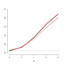
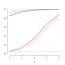
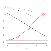
Figure 1: Observed frequencies of rejection for clean and contaminated samples under model M2 and the contiguous alternatives $H_{\Delta,n}^{(1)}$. The solid and dotted lines correspond to $n_{1}=n_{2}=100$ and $200$, respectively, while the dashed line to $n_{1}=200$ and $n_{2}=100$. The frequencies of rejection of $T_{n,\mbox{\footnotesize\sc cl}}$ and $T_{n,\mbox{\footnotesize\sc r}}$ are given in black and red, respectively.

$C_{0}$	$C_{3}$	$C_{4}$

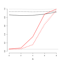
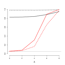
Figure 2: Observed frequencies of rejection for clean and contaminated samples under model M2 and the contiguous alternatives $H_{\Delta,n}^{(2)}$. The solid and dotted lines correspond to $n_{1}=n_{2}=100$ and $200$, respectively, while the dashed line to $n_{1}=200$ and $n_{2}=100$. The frequencies of rejection of $T_{n,\mbox{\footnotesize\sc cl}}$ and $T_{n,\mbox{\footnotesize\sc r}}$ are given in black and red, respectively.

$C_{0}$	$C_{3}$	$C_{4}$

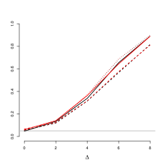
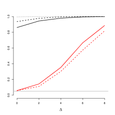
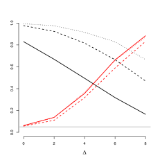
Figure 3: Observed frequencies of rejection for clean and contaminated samples under model M4 and the contiguous alternatives $H_{\Delta,n}^{(1)}$. The solid and dotted lines correspond to $n_{1}=n_{2}=100$ and $200$, respectively, while the dashed line to $n_{1}=200$ and $n_{2}=100$. The frequencies of rejection of $T_{n,\mbox{\footnotesize\sc cl}}$ and $T_{n,\mbox{\footnotesize\sc r}}$ are given in black and red, respectively.

The left panels of Figures 1 to 3 illustrate that both procedures have a similar performance under $C_{0}$ with a small loss of power when unbalanced designs are considered. The two contaminations considered do not affect the robust test introduced in this paper that still provides reliable results. Regarding the performance of the test based on $T_{n,\mbox{\footnotesize\sc cl}}$ under contamination, different behaviours can be described. When gross vertical outliers are introduced in both populations, the test becomes non–informative under the family of alternatives $H_{\Delta,n}^{(1)}$ with an almost constant frequency of rejection. The same effect on $T_{n,\mbox{\footnotesize\sc cl}}$ is observed under $C_{4}$ when considering the two–sided local alternatives $H_{\Delta,n}^{(2)}$. When considering the one–sided alternatives $H_{\Delta,n}^{(1)}$ and the contamination scheme $C_{4}$, a Hauck–Donner effect may be observed, since its power decreases almost to the level of significance as the alternative moves away from the null hypothesis, when $n_{1}=n_{2}=100$. We guess that the same effect would be observed for the other sample sizes when larger values of $\Delta$ are considered. In contrast, the two contaminations $C_{3}$ and $C_{4}$ considered do not affect the robust test introduced in this paper that still provides reliable results.

Figures 4 and 5 display the corresponding frequencies of rejection when the errors are heavy tailed. To facilitate comparisons the left panel in both Figures repeats the plot for normal errors already displayed in Figures 1 and 2. When the errors have a ${\mathcal{T}}_{2}$ distribution, the classical test shows a clear lack of power underperforming the robust method. For Cauchy errors, the classical method shows no power, as already described for fixed alternatives in Table 4 making the test unreliable. With respect to the behaviour of the robust test, even though some loss of power is observed, specially when the errors have a Cauchy distribution, the test still provides reliable results, since the empirical level is not affected (see Table 4) and the power increases with $\Delta$.

$N(0,1)$	${\mathcal{T}}_{2}$	${\mathcal{T}}_{1}$

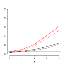
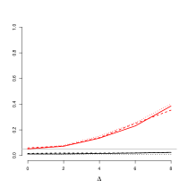
Figure 4: Observed frequencies of rejection for samples with normal and heavy tailed errors under model M2 and the contiguous alternatives $H_{\Delta,n}^{(1)}$. The solid and dotted lines correspond to $n_{1}=n_{2}=100$ and $200$, respectively, while the dashed line to $n_{1}=200$ and $n_{2}=100$. The frequencies of rejection of $T_{n,\mbox{\footnotesize\sc cl}}$ and $T_{n,\mbox{\footnotesize\sc r}}$ are given in black and red, respectively.

$N(0,1)$	${\mathcal{T}}_{2}$	${\mathcal{T}}_{1}$

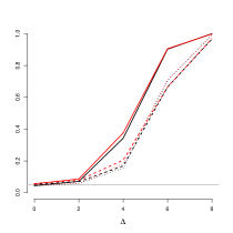
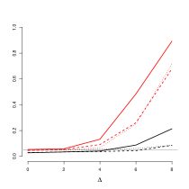
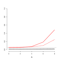
Figure 5: Observed frequencies of rejection for samples with normal and heavy tailed errors under model M2 and the contiguous alternatives $H_{\Delta,n}^{(2)}$. The solid and dotted lines correspond to $n_{1}=n_{2}=100$ and $200$, respectively, while the dashed line to $n_{1}=200$ and $n_{2}=100$. The frequencies of rejection of $T_{n,\mbox{\footnotesize\sc cl}}$ and $T_{n,\mbox{\footnotesize\sc r}}$ are given in black and red, respectively.

5 Real data analysis

In environmental studies the relation between rainfall and acid rain has been studied to decide the pollution impact. In this section, we consider a data set that was previously studied in Hall and Hart, (1990) and Neumeyer and Dette, (2003) which contains, the week, the amount of rainfall and the logarithm of the sulfate concentration along a five-year period 1979-1983 in two locations of North Carolina, Coweeta and Lewiston. For some weeks, data are not available, so we only have information on 215 weeks in Lewiston and on 220 weeks in Coweeta. As mentioned in Hall and Hart, (1990) the data were part of the National Atmospheric Deposition Program. Both Hall and Hart, (1990) and Neumeyer and Dette, (2003) used the data to compare the logarithm of acidity, i.e., the logarithm of the sulfate concentration previously adjusted for the amount of rainfall as a function of time in the two locations. In our analysis we are instead interested in the relation between the logarithm of the sulfate concentration and the rainfall, that is, the response variable is the logarithm of the sulfate concentration which was modelled nonparametrically as a function of the rainfall. From now on the observations corresponding to Coweeta are identified as $(X_{i1},Y_{i1})^{\mbox{\footnotesize\sc t}}$ and those of Lewiston as $(X_{i2},Y_{i2})^{\mbox{\footnotesize\sc t}}$, so that we deal with the regression model (1).

Figure 6 displays the observations corresponding to Coweeta and Lewiston. The upper plot presents the data in separate panels, while in the lower one the observations corresponding to Coweeta are shown in blue filled points and those related to Lewiston as red circles.

(a) Coweeta	(b) Lewiston
(c)

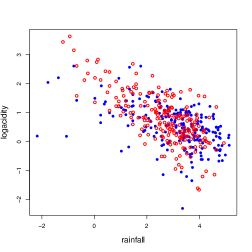
Figure 6: Scatterplot of the logarithm of the sulfate concentration (“logacidity”) versus rainfall. Panel (a) corresponds to the data recorded at Coweeta, while panel (b) to those in Lewiston. The lower panel (c) the observations at both locations are plotted jointly, the blue filled points and the red circles correspond to the measurements in Coweeta and Lewiston, respectively.

The fits obtained for each city using the classical and robust smoothers are given in Figure 7 together with the observations detected as atypical (in red triangles) using the boxplot of the residuals from the robust fit. The main differences between the two fits are observed in Coweeta for low values of rainfall. For the Nadaraya–Watson estimator the cross–validation bandwidths equal $h_{1}=1.6$ and $h_{2}=0.8$, while when using a local $M-$smoother and a robust cross-validation criterion, we obtain $h_{1}=1.3$ and $0.9$. The classical test statistic proposed in Pardo-Fernández et al., (2015) rejects at level 0.05 the null hypothesis with a $p-$value equal to $0.0496$, while the robust procedure does not detect differences between both locations ($p-$value= 0.1117).

(a) Coweeta	(b) Lewiston

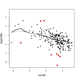
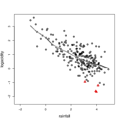
Figure 7: Scatterplot of the logarithm of the sulfate concentration (“logacidity”) versus rainfall together with the Nadaraya–Watson and robust smoothers in gray and black lines, respectively. The red triangles highlight the observations detected as atypical by the robust fit. Panel (a) corresponds to the data recorded at Coweeta, while panel (b) to those in Lewiston.

To detect the possible influence of the bandwidth choice on the resulting $p-$value, we choose a grid of values for $h_{1}$ and $h_{2}$ ranging in the range 0.7 to 1.8 and 0.6 to 1.6, respectively, with a step of 0.1. Figure 8 displays the surface of the obtained $p-$values. The left panel corresponds to the classical procedure which is based on empirical characteristic functions using the residuals from the Nadaraya–Watson smoother, while the right one to the method proposed in this paper. The obtained surfaces show that the decision taken by the test based on the statistic $T_{n,\mbox{\footnotesize\sc r}}$ is less dependent to the bandwidth choice, while the classical one leads to $p-$values varying from $0.035$ to $0.132$ changing the decision at 5% level. This effect can be explained by the effect that the observations, whose residuals from the robust fit are detected as outliers by the boxplot, have on the classical procedure.

(a)	(b)

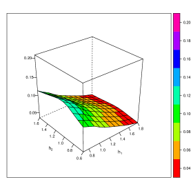
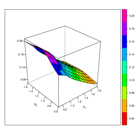
Figure 8: $p-$values as a function of the bandwidths used to estimate the regression functions. Panel (a) corresponds to the $p-$values obtained when using the procedure proposed in Pardo-Fernández et al., (2015) and panel (b) to those of the robust testing method defined in this paper.

6 Final Comments

In this paper we proposed and studied a new robust procedure to test equality of several regression curves in a nonparametric setup, which detects alternatives converging to the null hypothesis at the parametric rate $n^{-1/2}$. Our proposal adapts the ideas in Pardo-Fernández et al., (2015) by considering the empirical characteristic functions of the residuals obtained from a robust fit. In this way, first moment conditions for the errors distribution are avoided. The robust procedure introduced does not assume that the design points have the same density. Simulations have shown a good practical behaviour of the new test under different regression models and contamination settings. If no outliers are present in the sample, the behaviour of the new test is almost equal to that of the procedure given in Pardo-Fernández et al., (2015), but when outliers appear in the samples, the robust test clearly outperforms the latter. The influence of the smoothing parameter on the test $p-$values is also studied on a real data set, revealing that the robust testing procedure is more stable with respect to the bandwidth choice.

Acknowledgements. This research was partially supported by Grants 20020170100022BA from the Universidad de Buenos Aires and pict 2021-I-A-00260 from anpcyt at Buenos Aires, Argentina (G. Boente) and also by the Spanish Projects from the Ministry of Science and Innovation (MCIN/ AEI /10.13039/501100011033) PID2020-116587GB-I00. CoDyNP (G. Boente) and PID2020-118101GB-I00 (J. C. Pardo-Fernández). The research was begun while G. Boente was visiting the Universidade de Vigo supported by this last project.

A Appendix: Proofs

The following Lemma states an asymptotic distribution result that will be useful in the proof of Theorem 3.1.

Lemma A.1.

Assume that (1) and A1 to A3, A5 and A7a) hold. Define

$$Z_{n,j}=\frac{1}{\sigma_{j}}\pi_{j}^{1/2}\sum_{s=1}^{k}\frac{\sigma_{s}}{\nu_{s}}\pi_{s}^{1/2}\,\frac{1}{\sqrt{n_{s}}}\sum_{r=1}^{n_{s}}W_{j}(X_{sr})\frac{f_{j}(X_{sr})}{f(X_{sr})}\psi_{s}\left(\varepsilon_{sr}\right)-\frac{1}{\nu_{j}}\mathbb{E}\left(W_{j}(X_{j})\right)\frac{1}{\sqrt{n_{j}}}\sum_{s=1}^{n_{j}}\psi_{j}\left(\varepsilon_{js}\right)\,.$$

Then, $\mathbf{Z}_{n}=(Z_{n,1},\dots,Z_{n,k})^{\mbox{\footnotesize\sc t}}\buildrel D\over{\longrightarrow}N({\bf{0}},\mbox{\boldmath$\Sigma$})$ where $\Sigma$ is defined in Theorem 3.1.

Proof.

Note that

$$Z_{n,j} =\frac{1}{\sigma_{j}}\pi_{j}^{1/2}\sum_{s\neq j}\frac{\sigma_{s}}{\nu_{s}}\pi_{s}^{1/2}\,\frac{1}{\sqrt{n_{s}}}\sum_{r=1}^{n_{s}}W_{j}(X_{sr})\frac{f_{j}(X_{sr})}{f(X_{sr})}\psi_{s}\left(\varepsilon_{sr}\right)$$

$$+\frac{\pi_{j}}{\nu_{j}}\,\frac{1}{\sqrt{n_{j}}}\sum_{r=1}^{n_{j}}W_{j}(X_{jr})\frac{f_{j}(X_{jr})}{f(X_{jr})}\psi_{j}\left(\varepsilon_{jr}\right)-\frac{1}{\nu_{j}}\mathbb{E}\left(W_{j}(X_{j})\right)\frac{1}{\sqrt{n_{j}}}\sum_{s=1}^{n_{j}}\psi_{j}\left(\varepsilon_{js}\right)$$

$$=\sum_{s\neq j}\frac{\sigma_{s}}{\sigma_{j}}\frac{\pi_{j}^{1/2}\pi_{s}^{1/2}}{\nu_{s}}\,\frac{1}{\sqrt{n_{s}}}\sum_{r=1}^{n_{s}}W_{j}(X_{sr})\frac{f_{j}(X_{sr})}{f(X_{sr})}\psi_{s}\left(\varepsilon_{sr}\right)$$

$$+\frac{1}{\sqrt{n_{j}}}\sum_{r=1}^{n_{j}}\psi_{j}\left(\varepsilon_{jr}\right)\left[\frac{\pi_{j}}{\nu_{j}}W_{j}(X_{jr})\frac{f_{j}(X_{jr})}{f(X_{jr})}-\frac{\mathbb{E}\left(W_{j}(X_{j})\right)}{\nu_{j}}\right]\,.$$

Recall that $\nu_{j}=\mathbb{E}[\psi_{j}^{\prime}(\varepsilon_{j})]\neq 0$, $\tau_{j}=\mathbb{E}[\psi_{j}^{2}(\varepsilon_{j})]$, $e_{j}=\tau_{j}/\nu_{j}^{2}$ and $\mathbb{E}\psi_{j}(\varepsilon_{j})=0$. Then, using that the populations are independent we get that

$$\mbox{\sc Var}(Z_{n,j}) =\sum_{s\neq j}\pi_{j}\pi_{s}\,\frac{\sigma_{s}^{2}}{\sigma_{j}^{2}}\frac{\tau_{s}}{\nu_{s}^{2}}\mathbb{E}\left\{W_{j}^{2}(X_{s})\frac{f_{j}^{2}(X_{s})}{f^{2}(X_{s})}\right\}+\tau_{j}\mathbb{E}\left[\frac{\pi_{j}}{\nu_{j}}W_{j}(X_{j})\frac{f_{j}(X_{j})}{f(X_{j})}-\frac{\mathbb{E}\left(W_{j}(X_{j})\right)}{\nu_{j}}\right]^{2}$$

$$=\sum_{s\neq j}\pi_{j}\pi_{s}\,\frac{\sigma_{s}^{2}}{\sigma_{j}^{2}}\frac{\tau_{s}}{\nu_{s}^{2}}\mathbb{E}\left\{W_{j}^{2}(X_{s})\frac{f_{j}^{2}(X_{s})}{f^{2}(X_{s})}\right\}+\frac{\tau_{j}}{\nu_{j}^{2}}\mathbb{E}\left[\pi_{j}W_{j}(X_{j})\frac{f_{j}(X_{j})}{f(X_{j})}-\mathbb{E}\left(W_{j}(X_{j})\right)\right]^{2}$$

$$=\sum_{s\neq j}\pi_{j}\pi_{s}\,e_{s}\,\frac{\sigma_{s}^{2}}{\sigma_{j}^{2}}\mathbb{E}\left\{W_{j}^{2}(X_{s})\frac{f_{j}^{2}(X_{s})}{f^{2}(X_{s})}\right\}+e_{j}\mathbb{E}\left[\pi_{j}W_{j}(X_{j})\frac{f_{j}(X_{j})}{f(X_{j})}-\mathbb{E}\left(W_{j}(X_{j})\right)\right]^{2}$$

$$=\sum_{s=1}^{k}\pi_{j}\pi_{s}\,e_{s}\,\frac{\sigma_{s}^{2}}{\sigma_{j}^{2}}\mathbb{E}\left\{W_{j}^{2}(X_{s})\frac{f_{j}^{2}(X_{s})}{f^{2}(X_{s})}\right\}$$

$$-\pi_{j}^{2}\,e_{j}\,\mathbb{E}\left\{W_{j}^{2}(X_{j})\frac{f_{j}^{2}(X_{j})}{f^{2}(X_{j})}\right\}+e_{j}\mathbb{E}\left[\pi_{j}W_{j}(X_{j})\frac{f_{j}(X_{j})}{f(X_{j})}-\mathbb{E}\left(W_{j}(X_{j})\right)\right]^{2}$$

$$=\sum_{s=1}^{k}\pi_{j}\pi_{s}\,e_{s}\,\frac{\sigma_{s}^{2}}{\sigma_{j}^{2}}\mathbb{E}\left\{W_{j}^{2}(X_{s})\frac{f_{j}^{2}(X_{s})}{f^{2}(X_{s})}\right\}+e_{j}\left\{\left[\mathbb{E}W_{j}(X_{j})\right]^{2}-2\pi_{j}\mathbb{E}\left(W_{j}(X_{j})\right)\mathbb{E}\left[W_{j}(X_{j})\frac{f_{j}(X_{j})}{f(X_{j})}\right]\right\}\,.$$

Noting that

$$\alpha_{j}^{(s)}=\mathbb{E}\left\{W_{j}^{2}(X_{s})\frac{f_{j}^{2}(X_{s})}{f^{2}(X_{s})}\right\}\qquad\beta_{j}=\mathbb{E}\left\{W_{j}(X_{j})\frac{f_{j}(X_{j})}{f(X_{j})}\right\}\qquad\omega_{j}=\mathbb{E}W_{j}(X_{j})\,,$$

we obtain

$$\mbox{\sc Var}(Z_{n,j}) =\sum_{s=1}^{k}\pi_{j}\,\pi_{s}\,e_{s}\,\alpha_{j}^{(s)}\,\frac{\sigma_{s}^{2}}{\sigma_{j}^{2}}+e_{j}\left\{\omega_{j}^{2}-2\pi_{j}\omega_{j}\beta_{j}\right\}\;.$$

We now compute $\mbox{\sc Cov}(Z_{n,j},Z_{n,\ell})$, for $\ell\neq j$. Recall that

$$Z_{n,j} =\sum_{s\neq j}\frac{\sigma_{s}}{\sigma_{j}}\frac{\pi_{j}^{1/2}\pi_{s}^{1/2}}{\nu_{s}}\,\frac{1}{\sqrt{n_{s}}}\sum_{r=1}^{n_{s}}W_{j}(X_{sr})\frac{f_{j}(X_{sr})}{f(X_{sr})}\psi_{s}\left(\varepsilon_{sr}\right)+\frac{1}{\sqrt{n_{j}}}\sum_{r=1}^{n_{j}}\psi_{j}\left(\varepsilon_{jr}\right)\left[\frac{\pi_{j}}{\nu_{j}}W_{j}(X_{jr})\frac{f_{j}(X_{jr})}{f(X_{jr})}-\frac{\omega_{j}}{\nu_{j}}\right]$$

$$=\sum_{s\neq j,\ell}\frac{\sigma_{s}}{\sigma_{j}}\frac{\pi_{j}^{1/2}\pi_{s}^{1/2}}{\nu_{s}}\,\frac{1}{\sqrt{n_{s}}}\sum_{r=1}^{n_{s}}W_{j}(X_{sr})\frac{f_{j}(X_{sr})}{f(X_{sr})}\psi_{s}\left(\varepsilon_{sr}\right)$$

$$+\frac{\sigma_{\ell}}{\sigma_{j}}\frac{\pi_{j}^{1/2}\pi_{\ell}^{1/2}}{\nu_{\ell}}\,\frac{1}{\sqrt{n_{\ell}}}\sum_{r=1}^{n_{\ell}}W_{j}(X_{\ell r})\frac{f_{j}(X_{\ell r})}{f(X_{\ell r})}\psi_{\ell}\left(\varepsilon_{\ell r}\right)+\frac{1}{\sqrt{n_{j}}}\sum_{r=1}^{n_{j}}\psi_{j}\left(\varepsilon_{jr}\right)\left[\frac{\pi_{j}}{\nu_{j}}W_{j}(X_{jr})\frac{f_{j}(X_{jr})}{f(X_{jr})}-\frac{\omega_{j}}{\nu_{j}}\right]\,,$$

while

$$Z_{n,\ell} =\sum_{s\neq\ell}\frac{\sigma_{s}}{\sigma_{\ell}}\frac{\pi_{\ell}^{1/2}\pi_{s}^{1/2}}{\nu_{s}}\,\frac{1}{\sqrt{n_{s}}}\sum_{r=1}^{n_{s}}W_{\ell}(X_{sr})\frac{f_{\ell}(X_{sr})}{f(X_{sr})}\psi_{s}\left(\varepsilon_{sr}\right)+\frac{1}{\sqrt{n_{\ell}}}\sum_{r=1}^{n_{\ell}}\psi_{\ell}\left(\varepsilon_{\ell r}\right)\left[\frac{\pi_{\ell}}{\nu_{\ell}}W_{\ell}(X_{\ell r})\frac{f_{\ell}(X_{\ell r})}{f(X_{\ell r})}-\frac{\omega_{\ell}}{\nu_{\ell}}\right]$$

$$=\sum_{s\neq\ell,j}\frac{\sigma_{s}}{\sigma_{\ell}}\frac{\pi_{\ell}^{1/2}\pi_{s}^{1/2}}{\nu_{s}}\,\frac{1}{\sqrt{n_{s}}}\sum_{r=1}^{n_{s}}W_{\ell}(X_{sr})\frac{f_{\ell}(X_{sr})}{f(X_{sr})}\psi_{s}\left(\varepsilon_{sr}\right)$$

$$+\frac{\sigma_{j}}{\sigma_{\ell}}\frac{\pi_{j}^{1/2}\pi_{\ell}^{1/2}}{\nu_{j}}\,\frac{1}{\sqrt{n_{j}}}\sum_{r=1}^{n_{j}}W_{\ell}(X_{jr})\frac{f_{\ell}(X_{jr})}{f(X_{jr})}\psi_{j}\left(\varepsilon_{jr}\right)+\frac{1}{\sqrt{n_{\ell}}}\sum_{r=1}^{n_{\ell}}\psi_{\ell}\left(\varepsilon_{\ell r}\right)\left[\frac{\pi_{\ell}}{\nu_{\ell}}W_{\ell}(X_{\ell r})\frac{f_{\ell}(X_{\ell r})}{f(X_{\ell r})}-\frac{\omega_{\ell}}{\nu_{\ell}}\right]\,.$$

For simplicity, denote

$$A_{s,\ell} =\frac{\sigma_{s}}{\sigma_{\ell}}\frac{\pi_{\ell}^{1/2}\pi_{s}^{1/2}}{\nu_{s}}\,\frac{1}{\sqrt{n_{s}}}\sum_{r=1}^{n_{s}}W_{\ell}(X_{sr})\frac{f_{\ell}(X_{sr})}{f(X_{sr})}\psi_{s}\left(\varepsilon_{sr}\right)\,,$$

$$c_{j,\ell} =\mbox{\sc Cov}\left(\frac{\sigma_{\ell}}{\sigma_{j}}\frac{\pi_{j}^{1/2}\pi_{\ell}^{1/2}}{\nu_{\ell}}\,\frac{1}{\sqrt{n_{\ell}}}\sum_{r=1}^{n_{\ell}}W_{j}(X_{\ell r})\frac{f_{j}(X_{\ell r})}{f(X_{\ell r})}\psi_{\ell}\left(\varepsilon_{\ell r}\right),\frac{1}{\sqrt{n_{\ell}}}\sum_{r=1}^{n_{\ell}}\psi_{\ell}\left(\varepsilon_{\ell r}\right)\left[\frac{\pi_{\ell}}{\nu_{\ell}}W_{\ell}(X_{\ell r})\frac{f_{\ell}(X_{\ell r})}{f(X_{\ell r})}-\frac{\omega_{\ell}}{\nu_{\ell}}\right]\right)\,.$$

Then, we have that

$$\mbox{\sc Cov}(Z_{n,j},Z_{n,\ell}) =\mbox{\sc Cov}\left(\sum_{s\neq\ell,j}A_{s,\ell},\sum_{r\neq j,\ell}A_{r,j}\right)+c_{j,\ell}+c_{\ell,j}\,.$$ (A.1)

We begin by computing $\mbox{\sc Cov}\left(\sum_{s\neq\ell,j}A_{s,\ell},\sum_{r\neq j,\ell}A_{r,j}\right)$. Note that the samples independence entail that

$$\mbox{\sc Cov}\left(\sum_{s\neq\ell,j}A_{s,\ell},\sum_{r\neq j,\ell}A_{r,j}\right)=\sum_{s\neq\ell,j}\mbox{\sc Cov}\left(A_{s,\ell},A_{s,j}\right)$$

$$=\sum_{s\neq\ell,j}\mbox{\sc Cov}\left(\frac{\sigma_{s}}{\sigma_{\ell}}\frac{\pi_{s}^{1/2}\pi_{\ell}^{1/2}}{\nu_{s}}\,\frac{1}{\sqrt{n_{s}}}\sum_{r=1}^{n_{s}}W_{\ell}(X_{sr})\frac{f_{\ell}(X_{sr})}{f(X_{sr})}\psi_{s}\left(\varepsilon_{sr}\right),\frac{\sigma_{s}}{\sigma_{j}}\frac{\pi_{s}^{1/2}\pi_{j}^{1/2}}{\nu_{s}}\,\frac{1}{\sqrt{n_{s}}}\sum_{r=1}^{n_{s}}W_{j}(X_{sr})\frac{f_{j}(X_{sr})}{f(X_{sr})}\psi_{s}\left(\varepsilon_{sr}\right)\right)$$

$$=\frac{\pi_{\ell}^{1/2}\,\pi_{j}^{1/2}}{\sigma_{\ell}\,\sigma_{j}}\,\sum_{s\neq\ell,j}\frac{\pi_{s}\,\sigma_{s}^{2}}{\nu_{s}^{2}}\mbox{\sc Cov}\left(W_{\ell}(X_{s})\frac{f_{\ell}(X_{s})}{f(X_{s})}\psi_{s}\left(\varepsilon_{s}\right),W_{j}(X_{s})\frac{f_{j}(X_{s})}{f(X_{s})}\psi_{s}\left(\varepsilon_{s}\right)\right)\,.$$

Using again that $\mathbb{E}\psi_{j}(\varepsilon_{j})=0$ and that $\mathbb{E}\psi_{s}^{2}\left(\varepsilon_{s}\right)/\nu_{s}^{2}=e_{s}$ and that

$$\alpha_{j,\ell}^{(s)}=\mathbb{E}\left(\frac{W_{\ell}(X_{s})f_{\ell}(X_{s})\,W_{j}(X_{s})f_{j}(X_{s})}{f^{2}(X_{s})}\right)\,,$$

we get that

$$\mbox{\sc Cov}\left(\sum_{s\neq\ell,j}A_{s,\ell}\right. \left.,\sum_{r\neq j,\ell}A_{r,j}\right)=\frac{\pi_{\ell}^{1/2}\,\pi_{j}^{1/2}}{\sigma_{\ell}\,\sigma_{j}}\,\sum_{s\neq\ell,j}\frac{\pi_{s}\,\sigma_{s}^{2}}{\nu_{s}^{2}}\mathbb{E}\left(W_{\ell}(X_{s})W_{j}(X_{s})\frac{f_{\ell}(X_{s})\ f_{j}(X_{s})}{f^{2}(X_{s})}\psi_{s}^{2}\left(\varepsilon_{s}\right)\right)$$

$$=\frac{\pi_{\ell}^{1/2}\,\pi_{j}^{1/2}}{\sigma_{\ell}\,\sigma_{j}}\,\sum_{s\neq\ell,j}e_{s}\;\pi_{s}\,\sigma_{s}^{2}\mathbb{E}\left(\frac{W_{\ell}(X_{s})f_{\ell}(X_{s})\,W_{j}(X_{s})f_{j}(X_{s})}{f^{2}(X_{s})}\right)$$

$$=\frac{\pi_{\ell}^{1/2}\,\pi_{j}^{1/2}}{\sigma_{\ell}\,\sigma_{j}}\,\sum_{s\neq\ell,j}e_{s}\;\pi_{s}\,\sigma_{s}^{2}\alpha_{j,\ell}^{(s)}$$

$$=\frac{\pi_{\ell}^{1/2}\,\pi_{j}^{1/2}}{\sigma_{\ell}\,\sigma_{j}}\,\sum_{s=1}^{k}e_{s}\;\pi_{s}\,\sigma_{s}^{2}\alpha_{j,\ell}^{(s)}-\pi_{\ell}^{1/2}\,\pi_{j}^{1/2}\,\frac{\sigma_{\ell}}{\sigma_{j}}\,e_{\ell}\;\pi_{\ell}\,\alpha_{j,\ell}^{(\ell)}-\pi_{\ell}^{1/2}\,\pi_{j}^{1/2}\,\frac{\sigma_{j}}{\sigma_{\ell}}\,e_{j}\;\pi_{j}\alpha_{j,\ell}^{(j)}\,.$$ (A.2)

Let us compute $c_{j,\ell}$. Taking into account that $\mathbb{E}\psi_{\ell}\left(\varepsilon_{\ell}\right)=0$ and the independence between the errors and the covariates, we obtain

$$c_{j,\ell} =\mbox{\sc Cov}\left(\frac{\sigma_{\ell}}{\sigma_{j}}\frac{\pi_{j}^{1/2}\pi_{\ell}^{1/2}}{\nu_{\ell}}\,\frac{1}{\sqrt{n_{\ell}}}\sum_{r=1}^{n_{\ell}}W_{j}(X_{\ell r})\frac{f_{j}(X_{\ell r})}{f(X_{\ell r})}\psi_{\ell}\left(\varepsilon_{\ell r}\right),\frac{1}{\sqrt{n_{\ell}}}\sum_{r=1}^{n_{\ell}}\psi_{\ell}\left(\varepsilon_{\ell r}\right)\left[\frac{\pi_{\ell}}{\nu_{\ell}}W_{\ell}(X_{\ell r})\frac{f_{\ell}(X_{\ell r})}{f(X_{\ell r})}-\frac{\omega_{\ell}}{\nu_{\ell}}\right]\right)$$

$$=\mbox{\sc Cov}\left(\frac{\sigma_{\ell}}{\sigma_{j}}\frac{\pi_{j}^{1/2}\pi_{\ell}^{1/2}}{\nu_{\ell}}\,\frac{1}{\sqrt{n_{\ell}}}\sum_{r=1}^{n_{\ell}}W_{j}(X_{\ell r})\frac{f_{j}(X_{\ell r})}{f(X_{\ell r})}\psi_{\ell}\left(\varepsilon_{\ell r}\right),\frac{1}{\nu_{\ell}}\frac{1}{\sqrt{n_{\ell}}}\sum_{r=1}^{n_{\ell}}\psi_{\ell}\left(\varepsilon_{\ell r}\right)\left[\pi_{\ell}W_{\ell}(X_{\ell r})\frac{f_{\ell}(X_{\ell r})}{f(X_{\ell r})}-{\omega_{\ell}}\right]\right)$$

$$=\frac{\sigma_{\ell}}{\sigma_{j}}\frac{\pi_{j}^{1/2}\pi_{\ell}^{1/2}}{\nu_{\ell}^{2}}\,\mbox{\sc Cov}\left(W_{j}(X_{\ell})\frac{f_{j}(X_{\ell})}{f(X_{\ell})}\psi_{\ell}\left(\varepsilon_{\ell}\right),\psi_{\ell}\left(\varepsilon_{\ell}\right)\left[\pi_{\ell}W_{\ell}(X_{\ell})\frac{f_{\ell}(X_{\ell})}{f(X_{\ell})}-\omega_{\ell}\right]\right)$$

$$=\frac{\sigma_{\ell}}{\sigma_{j}}\frac{\pi_{j}^{1/2}\pi_{\ell}^{1/2}}{\nu_{\ell}^{2}}\,\mathbb{E}\left(\psi_{\ell}^{2}\left(\varepsilon_{\ell}\right)\right)\,\mathbb{E}\left(W_{j}(X_{\ell})\frac{f_{j}(X_{\ell})}{f(X_{\ell})}\left[\pi_{\ell}W_{\ell}(X_{\ell})\frac{f_{\ell}(X_{\ell})}{f(X_{\ell})}-\omega_{\ell}\right]\right)$$

$$=\frac{\sigma_{\ell}}{\sigma_{j}}\pi_{j}^{1/2}\,\pi_{\ell}^{1/2}\,e_{\ell}\,\left\{\pi_{\ell}\;\mathbb{E}\left(\frac{W_{j}(X_{\ell})f_{j}(X_{\ell})\;W_{\ell}(X_{\ell})f_{\ell}(X_{\ell})}{f^{2}(X_{\ell})}\right)-\omega_{\ell}\;\mathbb{E}\left(W_{j}(X_{\ell})\frac{f_{j}(X_{\ell})}{f(X_{\ell})}\right)\right\}$$

$$=\frac{\sigma_{\ell}}{\sigma_{j}}\pi_{j}^{1/2}\,\pi_{\ell}^{1/2}\,e_{\ell}\,\left\{\pi_{\ell}\;\alpha_{j,\ell}^{(\ell)}-\omega_{\ell}\;\beta_{j}^{(\ell)}\right\}\,,$$

where we have used that

$$\beta_{j}^{(\ell)}=\mathbb{E}\left\{W_{j}(X_{\ell})\frac{f_{j}(X_{\ell})}{f(X_{\ell})}\right\}\qquad\alpha_{j,\ell}^{(\ell)}=\mathbb{E}\left(\frac{W_{\ell}(X_{\ell})f_{\ell}(X_{\ell})\,W_{j}(X_{\ell})f_{j}(X_{\ell})}{f^{2}(X_{\ell})}\right)\,.$$

Summarizing we have that

$$c_{j,\ell} =\frac{\sigma_{\ell}}{\sigma_{j}}\pi_{j}^{1/2}\,\pi_{\ell}^{1/2}\,e_{\ell}\,\left\{\pi_{\ell}\;\alpha_{j,\ell}^{(\ell)}-\omega_{\ell}\;\beta_{j}^{(\ell)}\right\}=\frac{\sigma_{\ell}}{\sigma_{j}}\pi_{j}^{1/2}\,\pi_{\ell}^{1/2}\,\pi_{\ell}\;e_{\ell}\,\alpha_{j,\ell}^{(\ell)}-\frac{\sigma_{\ell}}{\sigma_{j}}\pi_{j}^{1/2}\,\pi_{\ell}^{1/2}\,e_{\ell}\,\omega_{\ell}\;\beta_{j}^{(\ell)}\,,$$

$$c_{\ell,j} =\frac{\sigma_{j}}{\sigma_{\ell}}\pi_{j}^{1/2}\,\pi_{\ell}^{1/2}\,e_{j}\,\left\{\pi_{j}\;\alpha_{j,\ell}^{(j)}-\omega_{j}\;\beta_{\ell}^{(j)}\right\}=\frac{\sigma_{j}}{\sigma_{\ell}}\pi_{j}^{1/2}\,\pi_{\ell}^{1/2}\,\pi_{j}\;e_{j}\,\alpha_{j,\ell}^{(j)}-\frac{\sigma_{j}}{\sigma_{\ell}}\pi_{j}^{1/2}\,\pi_{\ell}^{1/2}\,e_{j}\omega_{j}\;\beta_{\ell}^{(j)}\,,$$

which together with (A.2) and (A.1) leads to

$$\mbox{\sc Cov}(Z_{n,j},Z_{n,\ell}) =\mbox{\sc Cov}\left(\sum_{s\neq\ell,j}A_{s,\ell},\sum_{r\neq j,\ell}A_{r,j}\right)+c_{j,\ell}+c_{\ell,j}$$

$$=\frac{\pi_{\ell}^{1/2}\,\pi_{j}^{1/2}}{\sigma_{\ell}\,\sigma_{j}}\,\sum_{s=1}^{k}e_{s}\;\pi_{s}\,\sigma_{s}^{2}\alpha_{j,\ell}^{(s)}-\pi_{\ell}^{1/2}\,\pi_{j}^{1/2}\,\frac{\sigma_{\ell}}{\sigma_{j}}\,e_{\ell}\;\pi_{\ell}\,\alpha_{j,\ell}^{(\ell)}-\pi_{\ell}^{1/2}\,\pi_{j}^{1/2}\,\frac{\sigma_{j}}{\sigma_{\ell}}\,e_{j}\;\pi_{j}\alpha_{j,\ell}^{(j)}$$

$$\hskip-28.90755pt+\frac{\sigma_{\ell}}{\sigma_{j}}\pi_{j}^{1/2}\,\pi_{\ell}^{1/2}\,\pi_{\ell}\;e_{\ell}\,\alpha_{j,\ell}^{(\ell)}-\frac{\sigma_{\ell}}{\sigma_{j}}\pi_{j}^{1/2}\,\pi_{\ell}^{1/2}\,e_{\ell}\,\omega_{\ell}\;\beta_{j}^{(\ell)}+\frac{\sigma_{j}}{\sigma_{\ell}}\pi_{j}^{1/2}\,\pi_{\ell}^{1/2}\,\pi_{j}\;e_{j}\,\alpha_{j,\ell}^{(j)}-\frac{\sigma_{j}}{\sigma_{\ell}}\pi_{j}^{1/2}\,\pi_{\ell}^{1/2}\,e_{j}\omega_{j}\;\beta_{\ell}^{(j)}$$

$$=\frac{\pi_{\ell}^{1/2}\,\pi_{j}^{1/2}}{\sigma_{\ell}\,\sigma_{j}}\,\sum_{s=1}^{k}e_{s}\;\pi_{s}\,\sigma_{s}^{2}\alpha_{j,\ell}^{(s)}-\frac{\sigma_{\ell}}{\sigma_{j}}\pi_{j}^{1/2}\,\pi_{\ell}^{1/2}\,e_{\ell}\,\omega_{\ell}\;\beta_{j}^{(\ell)}-\frac{\sigma_{j}}{\sigma_{\ell}}\pi_{j}^{1/2}\,\pi_{\ell}^{1/2}\,e_{j}\omega_{j}\;\beta_{\ell}^{(j)}\,,$$

and the proof follows now from the multivariate central limit theorem. ∎

In the sequel we will use the consistency rates stated in Lemma A.2 which we include without proof. In the case of the robust regression estimator, the proof is a direct consequence of the results in Boente and Pardo-Fernández, (2016) combined with the bandwidth rate given in A8, while for the density estimator the result can be found in Pardo-Fernández et al., (2015).

From now on, given a sequence $\{a_{n}\}_{n\geq 1}$ a sequence of positive numbers and $\{V_{n}\}$ a sequence of random variables, $V_{n}=O_{a.co.}(a_{n})$ means that for some positive constant $C_{0}$, $\sum_{n\geq 1}\mathbb{P}(V_{n}>C_{0}a_{n})<\infty$.

Lemma A.2.

Define

$$\widehat{L}_{j}(x,\sigma) = \frac{1}{n_{j}}\sum_{\ell=1}^{n_{j}}\omega_{j\ell}(x)\psi_{j}\left(\frac{Y_{j\ell}-m_{j}(x)}{\sigma}\right)\,,$$ (A.3)

$\omega_{j\ell}(x)=K_{h}\left(x-X_{j\ell}\right)$ and $\theta_{n_{j}}=\sqrt{\log n_{j}/(n_{j}h)}$. Then, under conditions A1, A3, A4, A6 and A7a), for any compact set ${\mathcal{K}}\subset\accentset{\circ}{{\mathcal{R}}}$, we have

$$\sup_{x\in{\mathcal{K}}}|\widehat{m}_{j}(x)-m_{j}(x)|=O_{a.co.}\left(h^{2}+\theta_{n_{j}}\right)=o_{\mathbb{P}}(n_{j}^{-1/4})\,,$$ (A.4)

$$\sup_{x\in{\mathcal{K}}}\left|\widehat{m}_{j}(x)-m_{j}(x)-\frac{\widehat{\sigma}_{j}}{f_{j}(x)\nu_{j}}\,\widehat{L}_{j}(x,\widehat{\sigma}_{j})\right|=O_{a.co.}\left(h^{2}+\theta_{n_{j}}^{2}\right)=o_{\mathbb{P}}(n_{j}^{-1/2})\,,$$ (A.5)

$$\sup_{x\in{\mathcal{K}}}|\widehat{f}_{j}(x)-f_{j}(x)|=o_{\mathbb{P}}(n_{j}^{-1/4})\,.$$ (A.6)

A direct consequence of A7, (A.4) and (A.6) is that, under $H_{1,n}$,

$$\sup_{x\in{\mathcal{K}}}|\widehat{\mu}_{0}(x)-\mu_{0}(x)|=o_{\mathbb{P}}(n_{j}^{-1/4})\,,$$ (A.7)

where $\mu_{0}(x)$ and $\widehat{\mu}_{0}(x)$ are defined in (9) and (10), respectively. Note that under $H_{0}$, $\mu_{0}=m_{0}=m_{j}$, for all $j=1,\dots,k$, so that (A.7) follows immediately, while under the alternative $H_{1,n}$,

$$\mu_{0}(x)=m_{0}(x)+n^{-1/2}\sum_{j=1}^{k}\pi_{j}\,\frac{f_{j}(x)}{f(x)}\Delta_{j}(x)=m_{0}(x)+n^{-1/2}\Delta_{0}(x)\,.$$

Hence, we also have that

$$\sup_{x\in{\mathcal{K}}}|\widehat{\mu}_{0}(x)-m_{0}(x)|=o_{\mathbb{P}}(n_{j}^{-1/4})\,.$$ (A.8)

For the sake of simplicity, from now on, we denote $\widehat{\Delta}_{j}(x)=(\widehat{\mu}_{0}(x)-\widehat{m}_{j}(x))/{\widehat{\sigma}_{j}}$, $\widehat{\Upsilon}_{0,j}(x)=(\mu_{0}(x)-\widehat{\mu}_{0}(x))/{\widehat{\sigma}_{j}}$, $\widehat{\Upsilon}_{j}(x)=(m_{j}(x)-\widehat{m}_{j}(x))/{\widehat{\sigma}_{j}}$ and $\widehat{\Gamma}_{j}(x)=n^{-1/2}(\Delta_{j}(x)-\Delta_{0}(x))/{\widehat{\sigma}_{j}}$. Then,

$$\widehat{\Delta}_{j}(x)=-\widehat{\Upsilon}_{0,j}(x)+\widehat{\Upsilon}_{j}(x)-\widehat{\Gamma}_{j}(x)\,.$$ (A.9)

Lemma A.3.

Assume that (1) and A1 to A6, A7a) and A8 hold. Let $\widehat{\sigma}_{j}$ be a consistent estimator of $\sigma_{j}$, $j=1,\ldots,k$ satisfying A9 and let $\Delta_{j}:\mathbb{R}\to\mathbb{R}$ be such that $\mathbb{E}W_{j}(X_{j})\Delta_{j}^{2}(X_{j})<\infty$. Assume that $H_{1,n}:m_{j}=m_{0}+n^{-1/2}\Delta_{j}$ holds and define

$$D_{1,n_{j}}(t) =-\;\frac{1}{\sqrt{n_{j}}}\sum_{\ell=1}^{n_{j}}W_{j}(X_{j\ell})\,\exp(i\,t\,\widehat{\epsilon}_{0j\ell})\,\left\{\frac{\widehat{\mu}_{0}(X_{j\ell})-\widehat{m}_{j}(X_{j\ell})}{\widehat{\sigma}_{j}}\right\}^{2}\exp(i\,t\,\xi_{j\ell}^{(n)})\,,$$

$$D_{2,n_{j}}(t) =\frac{1}{\sqrt{n_{j}}}\sum_{\ell=1}^{n_{j}}W_{j}(X_{j\ell})\,\left[\widehat{\Upsilon}_{0,j}(X_{j\ell})+\widehat{\Gamma}_{j}(X_{j\ell})\right]\widehat{\Delta}_{j}(X_{j\ell})\exp(i\,t\,\xi_{j\ell}^{(n)})\,,$$

$$D_{3,n_{j}}(t) =\left(\frac{\widehat{\sigma}_{j}-\sigma_{j}}{\sigma_{j}}\right)\frac{1}{\sqrt{n_{j}}}\sum_{\ell=1}^{n_{j}}W_{j}(X_{j\ell})\,\exp\left\{i\,t\,\frac{\sigma_{j}}{\widehat{\sigma}_{j}}\varepsilon_{j\ell}\right\}\,\left\{\widehat{\Upsilon}_{j}(X_{j\ell})-\widehat{\Upsilon}_{0}(X_{j\ell})-\widehat{\Gamma}_{j}(X_{j\ell})\right\}\,,$$

where $\xi_{j\ell}^{(n)}$ are random variables that may depend on the sample size. Then, for $s=1,2,3$, we have that $\sup_{t\in\mathbb{R}}|D_{s,n_{j}}(t)|=o_{\mathbb{P}}(1)$

Proof.

Using that $m_{j}=m_{0}+n^{-1/2}\Delta_{j}$ and that $\mu_{0}(x)=m_{0}(x)+n^{-1/2}\Delta_{0}(x)$, we get that

$$\widehat{\mu}_{0}(x)-\widehat{m}_{j}(x) =\left(\widehat{\mu}_{0}(x)-m_{0}(x)\right)-\left(\widehat{m}_{j}(x)-m_{j}(x)\right)-n^{-1/2}\Delta_{j}(x)$$

$$=\left(\widehat{\mu}_{0}(x)-\mu_{0}(x)\right)-\left(\widehat{m}_{j}(x)-m_{j}(x)\right)+n^{-1/2}\left(\Delta_{0}(x)-\Delta_{j}(x)\right)\,,$$ (A.10)

which implies

$$\sup_{t\in\mathbb{R}}|D_{1,n_{j}}(t)| \leq\frac{1}{\sqrt{n_{j}}}\sum_{\ell=1}^{n_{j}}W_{j}(X_{j\ell})\,\frac{\left[\widehat{\mu}_{0}(X_{j\ell})-\widehat{m}_{j}(X_{j\ell})\right]^{2}}{\widehat{\sigma}_{j}^{2}}$$

$$\leq\frac{4}{\sqrt{n_{j}}\,\widehat{\sigma}_{j}^{2}}\sum_{\ell=1}^{n_{j}}W_{j}(X_{j\ell})\,\left\{\left[\widehat{\mu}_{0}(X_{j\ell})-m_{0}(X_{j\ell})\right]^{2}+\left[\widehat{m}_{j}(X_{j\ell})-m_{j}(X_{j\ell})\right]^{2}+\,n^{-1}\Delta_{j}^{2}(X_{j\ell})\right\}$$

$$\leq\frac{4}{\widehat{\sigma}_{j}^{2}}\left\{\sqrt{n_{j}}\sup_{x\in{\mathcal{S}}_{j}}\left[\widehat{\mu}_{0}(x)-m_{0}(x)\right]^{2}+\sqrt{n_{j}}\sup_{x\in{\mathcal{S}}_{j}}\left[\widehat{m}_{j}(x)-m_{j}(x)\right]^{2}\right\}$$

$$+\frac{4}{\widehat{\sigma}_{j}^{2}}\,\frac{n_{j}}{n}\,\frac{1}{\sqrt{n_{j}}}\,\left(\frac{1}{n_{j}}\sum_{\ell=1}^{n_{j}}W_{j}(X_{j\ell})\,\Delta_{j}^{2}(X_{j\ell})\right)\,.$$

From (A.4), taking ${\mathcal{K}}={\mathcal{S}}_{j}$, and using that $\widehat{\sigma}_{j}\buildrel p\over{\longrightarrow}\sigma_{j}$, $\mathbb{E}W_{j}(X_{j})\Delta_{j}^{2}(X_{j})<\infty$ and $n_{j}/n\to\kappa_{j}$, we easily get that $\sup_{t\in\mathbb{R}}|D_{1,n_{j}}(t)|=o_{\mathbb{P}}(1)$.

Let us show that $\sup_{t\in\mathbb{R}}|D_{2,n_{j}}(t)|=o_{\mathbb{P}}(1)$. Using (A.10) and denoting $A(x)=|\Delta_{0}(x)|+|\Delta_{j}(x)|$, $\widehat{A}_{0}=\sup_{x\in{\mathcal{S}}_{j}}\left|\widehat{\mu}_{0}(x)-\mu_{0}(x)\right|$ and $\widehat{A}_{j}=\sup_{x\in{\mathcal{S}}_{j}}\left|\widehat{m}_{j}(x)-m_{j}(x)\right|$, we can bound $\sup_{t\in\mathbb{R}}|D_{2,n_{j}}(t)|$ as

$$\sup_{t\in\mathbb{R}}|D_{2,n_{j}}(t)| \leq\frac{1}{\sqrt{n_{j}}}\sum_{\ell=1}^{n_{j}}W_{j}(X_{j\ell})\,\left|\widehat{\Upsilon}_{0,j}(X_{j\ell})+\widehat{\Gamma}_{j}(X_{j\ell})\right|\;\left|\widehat{\Delta}_{j}(X_{j\ell})\right|$$

$$\leq\frac{1}{\widehat{\sigma}_{j}^{2}}\frac{1}{\sqrt{n_{j}}}\sum_{\ell=1}^{n_{j}}W_{j}(X_{j\ell})\left|\mu_{0}(X_{j\ell})-\widehat{\mu}_{0}(X_{j\ell})+n^{-1/2}\left[\Delta_{j}(X_{j\ell})-\Delta_{0}(X_{j\ell})\right]\right|\;\left|\widehat{\mu}_{0}(X_{j\ell})-\widehat{m}_{j}(X_{j\ell})\right|$$

$$\leq\frac{1}{\widehat{\sigma}_{j}^{2}}\frac{1}{\sqrt{n_{j}}}\sum_{\ell=1}^{n_{j}}W_{j}(X_{j\ell})\left\{\left|\widehat{\mu}_{0}(X_{j\ell})-\mu_{0}(X_{j\ell})\right|\;+n^{-1/2}\;A(X_{j\ell})\right\}\;\times$$

$$\left\{\left|\widehat{\mu}_{0}(X_{j\ell})-\mu_{0}(X_{j\ell})\right|+\left|\widehat{m}_{j}(X_{j\ell})-m_{j}(X_{j\ell})\right|+n^{-1/2}A(X_{j\ell})\right\}$$

$$\leq\frac{1}{\widehat{\sigma}_{j}^{2}}\left\{\sqrt{n_{j}}\widehat{A}_{0}^{2}+2\,\widehat{A}_{0}\;\left(\frac{n_{j}}{n}\right)^{1/2}\,\frac{1}{n_{j}}\;\sum_{\ell=1}^{n_{j}}W_{j}(X_{j\ell})A(X_{j\ell})+\sqrt{n_{j}}\widehat{A}_{0}\widehat{A}_{j}\right.$$

$$\left.+\widehat{A}_{j}\;\left(\frac{n_{j}}{n}\right)^{1/2}\,\frac{1}{n_{j}}\;\sum_{\ell=1}^{n_{j}}W_{j}(X_{j\ell})A(X_{j\ell})+n^{-1/2}\left(\frac{n_{j}}{n}\right)^{1/2}\,\frac{1}{n_{j}}\;\sum_{\ell=1}^{n_{j}}W_{j}(X_{j\ell})A^{2}(X_{j\ell})\right\}\,.$$

Hence, using (A.4) and (A.8), together with the fact that $\mathbb{E}W_{j}(X_{j})\Delta_{j}^{2}(X_{j})<\infty$, we obtain that $\sup_{t\in\mathbb{R}}|D_{2,n_{j}}(t)|=o_{\mathbb{P}}(1)$.

Finally, to prove that $\sup_{t\in\mathbb{R}}|D_{3,n_{j}}(t)|=o_{\mathbb{P}}(1)$, note that

$$\sup_{t\in\mathbb{R}}|D_{3,n_{j}}(t)| \leq\left(\frac{|\widehat{\sigma}_{j}-\sigma_{j}|}{\widehat{\sigma}_{j}\,\sigma_{j}}\right)\frac{1}{\sqrt{n_{j}}}\sum_{\ell=1}^{n_{j}}W_{j}(X_{j\ell})\,\Big{\{}\left|\widehat{\mu}_{0}(X_{j\ell})-\mu_{0}(X_{j\ell})\right|+\left|\widehat{m}_{j}(X_{j\ell})-m_{j}(X_{j\ell})\right|$$

$$+n^{-1/2}\left|\Delta_{j}(X_{j\ell})-\Delta_{0}(X_{j\ell})\right|\Big{\}}$$

$$\leq\left(\frac{|\widehat{\sigma}_{j}-\sigma_{j}|}{\widehat{\sigma}_{j}\,\sigma_{j}}\right)\sqrt{n_{j}}\left(\widehat{A}_{0}+\widehat{A}_{j}\right)$$

$$+\left(\frac{|\widehat{\sigma}_{j}-\sigma_{j}|}{\widehat{\sigma}_{j}\,\sigma_{j}}\right)\left(\frac{n_{j}}{n}\right)^{1/2}\,\frac{1}{n_{j}}\;\sum_{\ell=1}^{n_{j}}W_{j}(X_{j\ell})\left|\Delta_{j}(X_{j\ell})-\Delta_{0}(X_{j\ell})\right|\,.$$ (A.11)

Using the consistency of $\widehat{\sigma}_{j}$ and the fact that $\mathbb{E}W_{j}(X_{j})\Delta_{j}^{2}(X_{j})<\infty$, we obtain that the second term on the right hand side of (A.11) converges to 0 in probability, while (A.4) and (A.8) together with the fact that ${n_{j}}^{1/4}(\widehat{\sigma}_{j}-\sigma_{j})=o_{\mathbb{P}}(1)$ entail that the first term is $o_{\mathbb{P}}(1)$, concluding the proof. ∎

Lemma A.4.

Assume that (1) and A1 to A8 hold. Let $\widehat{\sigma}_{j}$ be a consistent estimator of $\sigma_{j}$, $j=1,\ldots,k$ satisfying A9 and consider functions $\Delta_{j}:\mathbb{R}\to\mathbb{R}$ such that $\mathbb{E}W_{j}(X_{j})\Delta_{j}^{2}(X_{j})<\infty$. Assume that $H_{1,n}:m_{j}=m_{0}+n^{-1/2}\Delta_{j}$ holds. Denote $V_{s}(x)=(n_{s}/n)(f_{s}(x)/f(x))$, $M_{s}(x)=m_{s}(x)/f(x)$ and $C_{s}(x)=(n_{s}/n)M_{s}(x)$. Furthermore, define

$$D_{1,n_{j}}(\sigma,t) =\frac{1}{\sigma_{j}}\,\left(\frac{n_{j}}{n}\right)^{1/2}\,\frac{1}{n_{j}}\sum_{\ell=1}^{n_{j}}W_{j}(X_{j\ell})\,\exp\left\{i\,t\,\frac{\sigma_{j}}{\sigma}\varepsilon_{j\ell}\right\}(\Delta_{j}(X_{j\ell})-\Delta_{0}(X_{j\ell}))\,,$$

$$D_{2,n_{j}}(\sigma,t) =\frac{1}{\sigma_{j}}\frac{1}{\sqrt{n_{j}}}\sum_{\ell=1}^{n_{j}}W_{j}(X_{j\ell})\,\exp\left\{i\,t\,\frac{\sigma_{j}}{\sigma}\varepsilon_{j\ell}\right\}\,\left\{\widehat{m}_{j}(X_{j\ell})-m_{j}(X_{j\ell})\right\}\,,$$

$$D_{3,n_{j}}(\sigma,t) =\sum_{s=1}^{k}\frac{1}{\sigma_{j}}\frac{1}{\sqrt{n_{j}}}\sum_{\ell=1}^{n_{j}}W_{j}(X_{j\ell})V_{s}(X_{j\ell})\,\exp\left\{i\,t\,\frac{\sigma_{j}}{\sigma}\varepsilon_{j\ell}\right\}\,\left\{\widehat{m}_{s}(X_{j\ell})-m_{s}(X_{j\ell})\right\}\,,$$

$$D_{4,n_{j}}(\sigma,t) =\sum_{s=1}^{k}\frac{1}{\sigma_{j}}\frac{1}{\sqrt{n_{j}}}\sum_{\ell=1}^{n_{j}}W_{j}(X_{j\ell})C_{s}(X_{j\ell})\,\exp\left\{i\,t\,\frac{\sigma_{j}}{\sigma}\varepsilon_{j\ell}\right\}\,\left\{\widehat{f}_{s}(X_{j\ell})-f_{s}(X_{j\ell})\right\}\,,$$

$$D_{5,n_{j}}(\sigma,t) =\sum_{s=1}^{k}\frac{1}{\sigma_{j}}\frac{1}{\sqrt{n_{j}}}\sum_{\ell=1}^{n_{j}}W_{j}(X_{j\ell})V_{s}(X_{j\ell})M_{s}(X_{j\ell})\,\exp\left\{i\,t\,\frac{\sigma_{j}}{\sigma}\varepsilon_{j\ell}\right\}\,\left\{\widehat{f}(X_{j\ell})-f(X_{j\ell})\right\}\,.$$

1. If $\widehat{D}(t)=i\,t\,\left(D_{1,n_{j}}(\widehat{\sigma}_{j},t)-D_{1,n_{j}}(\sigma_{j},t)\right)$, then $\|\widehat{D}\|_{w}=o_{\mathbb{P}}(1)$.

2. Moreover, if A10 holds, we have that, for $s=1,\dots,5$, $D_{s,n_{j}}(\widehat{\sigma}_{j},t)=D_{s,n_{j}}(\sigma_{j},t)+i\,t\,R_{s,n_{j}}(t)$, where $\sup_{t\in\mathbb{R}}|R_{s,n_{j}}(t)|=o_{\mathbb{P}}(1)$.

Proof.

We begin by proving b). Using a Taylor’s expansion of order one, we obtain that

$$D_{1,n_{j}}(\widehat{\sigma}_{j},t)-D_{1,n_{j}}(\sigma_{j},t) =i\,t\,\frac{1}{\sigma_{j}}\,\left(\frac{\sigma_{j}}{\widehat{\sigma}_{j}}-1\right)\left(\frac{n_{j}}{n}\right)^{1/2}\,\frac{1}{n_{j}}\sum_{\ell=1}^{n_{j}}W_{j}(X_{j\ell})\,\exp\left\{i\,t\,\xi_{j\ell}\varepsilon_{j\ell}\right\}(\Delta_{j}(X_{j\ell})-\Delta_{0}(X_{j\ell}))\varepsilon_{j\ell}$$

$$=i\,t\,R_{1,n_{j}}(t)\,,$$

with $\xi_{j\ell}$ and intermediate point. Hence, noting that

$$\sup_{t\in\mathbb{R}}|R_{1,n_{j}}(t)| \leq\left(\frac{n_{j}}{n}\right)^{1/2}\,\frac{1}{\widehat{\sigma}_{j}\,\sigma_{j}}\,n_{j}^{1/\theta_{0}-1}\left|{\widehat{\sigma}_{j}}-{\sigma_{j}}\right|\,\frac{1}{n_{j}^{1/\theta_{0}}}\sum_{\ell=1}^{n_{j}}|\varepsilon_{j\ell}|\,W_{j}(X_{j\ell})\,\left|\Delta_{j}(X_{j\ell})-\Delta_{0}(X_{j\ell})\right|\,.$$

Using that $\mathbb{E}|\varepsilon_{j}|^{\theta_{0}}$, $W_{j}$ is bounded and $\Delta_{j}$ is bounded in the support of $W_{j}$, we get that $\mathbb{E}|Z_{j}|^{\theta_{0}}<\infty$, where $Z_{j}=|\varepsilon_{j}|\,W_{j}(X_{j})\,\left|\Delta_{j}(X_{j})-\Delta_{0}(X_{j})\right|$. Thus, from the Marcinkiewicz–Zygmund strong law of large numbers, see Appendix A in Shao and Tu, (1995), we get that

$$\frac{1}{n_{j}^{1/\theta_{0}}}\sum_{\ell=1}^{n_{j}}|\varepsilon_{j\ell}|\,W_{j}(X_{j\ell})\,\left|\Delta_{j}(X_{j\ell})-\Delta_{0}(X_{j\ell})\right|\buildrel a.s.\over{\longrightarrow}0\,,$$

which together with the facts that ${1/\theta_{0}-1}=\gamma_{0}-1/4$ and $n^{\gamma_{0}}(\widehat{\sigma}_{j}-\sigma_{j})=O_{\mathbb{P}}(1)$, imply that $\sup_{t\in\mathbb{R}}|R_{1,n_{j}}(t)|=o_{\mathbb{P}}(1)$.

Note that $D_{2,n_{j}}(\widehat{\sigma}_{j},t)-D_{2,n_{j}}(\sigma_{j},t)=i\,tR_{2,n_{j}}(t)$, where

$$R_{2,n_{j}}(t) =\frac{1}{\sigma_{j}}\frac{1}{\sqrt{n_{j}}}\sum_{\ell=1}^{n_{j}}W_{j}(X_{j\ell})\,\exp\left\{i\,t\,\xi_{j\ell}\right\}\,\left(\frac{\sigma_{j}}{\widehat{\sigma}_{j}}-1\right)\varepsilon_{j\ell}\left\{\widehat{m}_{j}(X_{j\ell})-m_{j}(X_{j\ell})\right\}\,,$$

with $\xi_{j\ell}$ an intermediate point. We have the following bound for $R_{2,n_{j}}(t)$

$$\left|R_{2,n_{j}}(t)\right| =\left|\frac{1}{\sigma_{j}}\frac{1}{\sqrt{n_{j}}}\sum_{\ell=1}^{n_{j}}W_{j}(X_{j\ell})\,\exp\left\{i\,t\,\xi_{j\ell}\right\}\,\left(\frac{\sigma_{j}}{\widehat{\sigma}_{j}}-1\right)\varepsilon_{j\ell}\left\{\widehat{m}_{j}(X_{j\ell})-m_{j}(X_{j\ell})\right\}\right|$$

$$\leq\frac{1}{\sigma_{j}}\sup_{x\in{\mathcal{S}}_{j}}\left|\widehat{m}_{j}(x)-m_{j}(x)\right|\;\left|\frac{\sigma_{j}}{\widehat{\sigma}_{j}}-1\right|\frac{1}{\sqrt{n_{j}}}\sum_{\ell=1}^{n_{j}}W_{j}(X_{j\ell})\left|\varepsilon_{j\ell}\right|$$

$$\leq\frac{1}{\widehat{\sigma}_{j}\,\sigma_{j}}n_{j}^{1/4}\sup_{x\in{\mathcal{S}}_{j}}\left|\widehat{m}_{j}(x)-m_{j}(x)\right|\;n_{j}^{\gamma_{0}}\left|\sigma_{j}-\widehat{\sigma}_{j}\right|\frac{1}{n_{j}^{1/\theta_{0}}}\sum_{\ell=1}^{n_{j}}\left|\varepsilon_{j\ell}\right|\,,$$

where in the last inequality we have used that $1/\theta_{0}-\gamma_{0}-1/4=1/2$. Therefore, using again that $\mathbb{E}|\varepsilon_{j}|^{\theta_{0}}$, the Marcinkiewicz–Zygmund strong law of large numbers, that $n^{\gamma_{0}}(\widehat{\sigma}_{j}-\sigma_{j})=O_{\mathbb{P}}(1)$, (A.4) and A9, we obtain that $\sup_{t\in\mathbb{R}}|R_{2,n_{j}}(t)|=o_{\mathbb{P}}(1)$ as desired. Similarly, using (A.4), A5, A9 and the fact that $\mathbb{E}|\varepsilon_{j}|^{\theta_{0}}<\infty$, we obtain that $D_{3,n_{j}}(\widehat{\sigma}_{j},t)=D_{3,n_{j}}(\sigma_{j},t)+i\,t\,R_{3,n_{j}}(t)$, where $\sup_{t\in\mathbb{R}}|R_{3,n_{j}}(t)|=o_{\mathbb{P}}(1)$. Finally, using (A.6), similar arguments allow to conclude that, for $s=4,5$, $D_{s,n_{j}}(\widehat{\sigma}_{j},t)=D_{s,n_{j}}(\sigma_{j},t)+i\,t\,R_{s,n_{j}}(t)$, where $\sup_{t\in\mathbb{R}}|R_{s,n_{j}}(t)|=o_{\mathbb{P}}(1)$.

Let us show a). Denote $D_{1,n_{j}}^{(1)}(t)=D_{1,n_{j}}(\widehat{\sigma}_{j},t)-D_{1,n_{j}}(\sigma_{j},t)$. Then, for any $M>0$,

$$D_{1,n_{j}}^{(1)}(t)=\frac{1}{\sigma_{j}}\,\left(\frac{n_{j}}{n}\right)^{1/2}\left(D_{1,n_{j}}^{(2)}(M,t)+D_{1,n_{j}}^{(3)}(M,t)\right)\,,$$ (A.12)

with

$$D_{1,n_{j}}^{(2)}(M,t) =\frac{1}{n_{j}}\sum_{\ell=1}^{n_{j}}U(X_{j\ell})\,\left\{\exp\left\{i\,t\,\frac{\sigma_{j}}{\widehat{\sigma}_{j}}\varepsilon_{j\ell}\right\}-\exp\left\{i\,t\,\varepsilon_{j\ell}\right\}\right\}\mathbb{I}_{|\varepsilon_{j\ell}|\leq M}\,,$$

$$D_{1,n_{j}}^{(3)}(M,t) =\frac{1}{n_{j}}\sum_{\ell=1}^{n_{j}}U(X_{j\ell})\,\left\{\exp\left\{i\,t\,\frac{\sigma_{j}}{\widehat{\sigma}_{j}}\varepsilon_{j\ell}\right\}-\exp\left\{i\,t\,\varepsilon_{j\ell}\right\}\right\}\mathbb{I}_{|\varepsilon_{j\ell}|\geq M}\,,$$

where for the sake of simplicity we have denoted $U(x)=W_{j}(x)\left(\Delta_{j}(x)-\Delta_{0}(x)\right)$. Note that

$$A_{1,n_{j}}(M)=\|i\,t\,D_{1,n_{j}}^{(3)}(M,t)\|_{w} \leq 2\frac{1}{n_{j}}\sum_{\ell=1}^{n_{j}}|U(X_{j\ell})|\mathbb{I}_{|\varepsilon_{j\ell}|\geq M}\left\{\int t^{2}w(t)\,dt\right\}^{1/2}\,,$$

while

$$\sup_{t\in\mathbb{R}}|D_{3,n_{j}}^{(2)}(M,t)|\leq M\left|\frac{\sigma_{j}}{\widehat{\sigma}_{j}}-1\right|\,\frac{1}{n_{j}}\sum_{\ell=1}^{n_{j}}\,\left|U(X_{j\ell})\right|\,,$$

so that

$$A_{2,n_{j}}(M)=\|i\,t\,D_{1,n_{j}}^{(2)}(M,t)\|_{w}\leq M\left|\frac{\sigma_{j}}{\widehat{\sigma}_{j}}-1\right|\,\frac{1}{n_{j}}\sum_{\ell=1}^{n_{j}}\,\left|U(X_{j\ell})\right|\left\{\int t^{2}w(t)\,dt\right\}^{1/2}\,.$$ (A.13)

Given $\delta>0$, choose $M$ such that $\left\{\int t^{2}w(t)\,dt\right\}^{1/2}\,\mathbb{E}|U(X_{j})|\mathbb{P}(|\varepsilon_{j}|>M)<\delta/(8a_{j})$, where $a_{j}=\pi_{j}^{1/2}/{\sigma_{j}}$. The law of large numbers entail that

$$A_{1,n_{j}}(M)\buildrel p\over{\longrightarrow}2\left\{\int t^{2}w(t)\,dt\right\}^{1/2}\,\mathbb{E}|U(X_{j})|\mathbb{P}(|\varepsilon_{j}|>M)<\delta/(4a_{j})\,,$$

so that, given $\eta>0$, there exists $n_{j,0}$ such that for $n_{j}\geq n_{j,0}$, we have that

$$\mathbb{P}\left(A_{1,n_{j}}(M)<\delta/(2a_{j})\right)>1-\eta/2\;.$$ (A.14)

On the other hand, the consistency of $\widehat{\sigma}_{j}$ together with the fact that $\mathbb{E}|U(X_{j})|<\infty$ entail that

$$A_{3,n_{j}}=\left|\frac{\sigma_{j}}{\widehat{\sigma}_{j}}-1\right|\,\frac{1}{n_{j}}\sum_{\ell=1}^{n_{j}}\,\left|U(X_{j\ell})\right|\left\{\int t^{2}w(t)\,dt\right\}^{1/2}\buildrel p\over{\longrightarrow}0\,,$$

therefore, we can choose $n_{j,1}$ such that for $n_{j}\geq n_{j,1}$, we have that $\mathbb{P}\left(A_{3,n_{j}}<\delta/(2\,M\,a_{j})\right)>1-\eta/2$, implying that

$$\mathbb{P}\left(A_{2,n_{j}}(M)<\delta/(2a_{j})\right)>1-\eta/2\;.$$ (A.15)

Taking into account that $n_{j}/n\to\pi_{j}$, we get that

$$a_{j,n_{j}}=\frac{1}{\sigma_{j}}\,\left(\frac{n_{j}}{n}\right)^{1/2}\to\frac{1}{\sigma_{j}}\,\pi_{j}^{1/2}=a_{j}\,,$$

so for $n_{j}\geq n_{j,2}$, we have that $a_{j,n_{j}}\leq 2a_{j}$. Combining (A.12), (A.13), (A.14) and (A.15), we obtain that for $n_{j}\geq\max(n_{j,0},n_{j,1},n_{j,2})$, $\mathbb{P}(\|\widehat{D}\|_{w}<\delta)>1-\eta$, which entails that $\|\widehat{D}\|_{w}=o_{\mathbb{P}}(1)$ concluding the proof. ∎

Lemma A.5.

Assume that (1) and A1 to A6, A7a) and A8 hold. Define for $s=1,\ldots,k$,

$$A_{1,s,n_{j}}(t) =\frac{1}{\sqrt{n_{j}}}\sum_{\ell=1}^{n_{j}}W_{j}(X_{j\ell})M_{s}(X_{j\ell})\,\exp\left\{i\,t\,\varepsilon_{j\ell}\right\}\,\left\{\widehat{f}_{s}(X_{j\ell})-f_{s}(X_{j\ell})\right\}\,,$$

$$A_{2,s,n_{j}}(t) =\frac{1}{\sqrt{n_{j}}}\sum_{\ell=1}^{n_{j}}W_{j}(X_{j\ell})V_{s}(X_{j\ell})M_{s}(X_{j\ell})\,\exp\left\{i\,t\,\varepsilon_{j\ell}\right\}\,\left\{\widehat{f}(X_{j\ell})-f(X_{j\ell})\right\}\,,$$

where $V_{s}(x)=(n_{s}/n)(f_{s}(x)/f(x))$, $M_{s}(x)=m_{s}(x)/f(x)$. Then, we have that $\sup_{t\in\mathbb{R}}|A_{\ell,s,n_{j}}(t)|=o_{\mathbb{P}}(1)$, for $\ell=1,2$.

Proof.

We will only show that $\sup_{t\in\mathbb{R}}|A_{1,s,n_{j}}(t)|=o_{\mathbb{P}}(1)$, since the proof of $\sup_{t\in\mathbb{R}}|A_{2,s,n_{j}}(t)|=o_{\mathbb{P}}(1)$ is analogous. Denote

$$f_{h,s}(x)=\mathbb{E}\widehat{f}_{s}(x)=\frac{1}{h}\int K\left(\frac{x-u}{h}\right)f_{s}(u)du=\frac{1}{h}\int K\left(\frac{x-u}{h}\right)\left\{f_{s}(u)-f_{s}(x)\right\}du+f_{s}(x)=r_{h,s}(x)+f_{s}(x)\,.$$

Recall that A5 and A6 imply that for $x\in{\mathcal{S}}_{j}$,

$$r_{h,s}(x) =\int K\left(v\right)\left\{f_{s}(x-h\,v)-f_{s}(x)\right\}dv=-hf_{s}^{\prime}(x)\int v\,K\left(v\right)dv+h^{2}\int v^{2}\,K\left(v\right)f_{s}^{\prime\prime}(\xi_{v,x})dv$$

$$=h^{2}\int v^{2}\,K\left(v\right)f_{s}^{\prime\prime}(\xi_{v,x})dv\,,$$

where $\xi_{v,x}$ is an intermediate point between $x$ and $x-h\,v$. Using that $f_{s}^{\prime\prime}$ is a continuous function in a neighbourhood of ${\mathcal{S}}_{j}$, we get that, for $h$ small enough, $\sup_{x\in{\mathcal{S}}_{j},v}|f_{s}^{\prime\prime}(\xi_{v,x})|=a_{j,s}<\infty$, so

$$\sup_{x\in{\mathcal{S}}_{j}}|r_{h,s}(x)|\leq h^{2}a_{j,s}\int v^{2}\,K\left(v\right)dv\,.$$ (A.16)

Then, $A_{1,s,n_{j}}(t)=B_{1,s,n_{j}}(t)+B_{2,s,n_{j}}(t)$ where

$$B_{1,s,n_{j}}(t) =\frac{1}{\sqrt{n_{j}}}\sum_{\ell=1}^{n_{j}}W_{j}(X_{j\ell})M_{s}(X_{j\ell})\,\exp\left\{i\,t\,\varepsilon_{j\ell}\right\}\,\left\{\widehat{f}_{s}(X_{j\ell})-f_{h,s}(X_{j\ell})\right\}\,,$$

$$B_{2,s,n_{j}}(t) =\frac{1}{\sqrt{n_{j}}}\sum_{\ell=1}^{n_{j}}W_{j}(X_{j\ell})M_{s}(X_{j\ell})\,\exp\left\{i\,t\,\varepsilon_{j\ell}\right\}\,r_{h,s}(X_{j\ell})\,.$$

Using (A.16) and that $\|W_{j}\|_{\infty}=1$, A4 and A5, we get that

$$\sup_{t\in\mathbb{R}}|B_{2,s,n_{j}}(t)|\leq\sqrt{n_{j}}\,h^{2}\,a_{j,s}A_{j,s}\,\int v^{2}\,K\left(v\right)dv\,,$$

where $A_{j,s}$ is an upper bound of $|M_{s}(u)|$ in a neighbourhood of ${\mathcal{S}}_{j}$. Hence, the fact that $n\,h^{4}\to 0$ entails that $\sup_{t\in\mathbb{R}}|B_{2,s,n_{j}}(t)|=o_{\mathbb{P}}(1)$.

Let us consider the situation $s\neq j$. In this case,

$$B_{1,s,n_{j}}(t) =\frac{1}{\sqrt{n_{j}}}\sum_{\ell=1}^{n_{j}}W_{j}(X_{j\ell})M_{s}(X_{j\ell})\,\exp\left\{i\,t\,\varepsilon_{j\ell}\right\}\,\left\{\widehat{f}_{s}(X_{j\ell})-f_{h,s}(X_{j\ell})\right\}$$

$$=\frac{1}{\sqrt{n_{j}}}\frac{1}{n_{s}}\sum_{\ell=1}^{n_{j}}\sum_{r=1}^{n_{s}}W_{j}(X_{j\ell})M_{s}(X_{j\ell})\,\exp\left\{i\,t\,\varepsilon_{j\ell}\right\}\left\{K_{h}\left(X_{j\ell}-X_{sr}\right)-f_{h,s}(X_{j\ell})\right\}$$

$$=B_{1,s,n_{j}}^{(1)}(t)+i\;B_{1,s,n_{j}}^{(2)}(t)\,.$$

Using that $\mathbb{E}\left\{K_{h}\left(X_{j}-X_{s}\right)-f_{h,s}(X_{j})\right\}=0$, standard arguments allow to show that, for $j=1,\ldots,k$, $\sup_{t\in\mathbb{R}}\mathbb{E}\{(B_{1,s,n_{j}}^{(j)}(t))^{2}\}=o(1)\,.$ Hence, $\|B_{1,s,n_{j}}\|_{w}=o_{\mathbb{P}}(1)$.

Let us consider the situation $s=j$. In this case, $B_{1,s,n_{j}}(t)=C_{1,n_{j}}(t)+C_{2,n_{j}}(t)$ where

$$C_{1,n_{j}}(t) =\frac{1}{n_{j}\sqrt{n_{j}}}\sum_{\ell=1}^{n_{j}}W_{j}(X_{j\ell})M_{s}(X_{j\ell})\,\exp\left\{i\,t\,\varepsilon_{j\ell}\right\}\left\{K_{h}\left(0\right)-f_{h,j}(X_{j\ell})\right\}\,,$$

$$C_{2,n_{j}}(t) =\frac{1}{n_{j}\sqrt{n_{j}}}\sum_{\ell\neq r}W_{j}(X_{j\ell})M_{s}(X_{j\ell})\,\exp\left\{i\,t\,\varepsilon_{j\ell}\right\}\left\{K_{h}\left(X_{j\ell}-X_{jr}\right)-f_{h,j}(X_{j\ell})\right\}$$

$$=\frac{1}{2n_{j}\sqrt{n_{j}}}\sum_{\ell\neq r}H(t,X_{j\ell},\varepsilon_{j\ell};X_{jr})+H(t,X_{jr},\varepsilon_{jr};X_{j\ell})\,,$$

where

$$H(t,X_{j\ell},\varepsilon_{j\ell};X_{jr})=W_{j}(X_{j\ell})M_{s}(X_{j\ell})\,\exp\left\{i\,t\,\varepsilon_{j\ell}\right\}\left\{K_{h}\left(X_{j\ell}-X_{jr}\right)-f_{h,j}(X_{j\ell})\right\}\,.$$

The fact that $nh^{2}\to\infty$ implies that $\sup_{t\in\mathbb{R}}|C_{1,n_{j}}(t)|=o_{\mathbb{P}}(1)$. Using similar arguments to those considered in Pardo-Fernández et al., (2015) for $B_{1,s,n_{j}}(t)$, we conclude that $\|C_{1,n_{j}}\|_{w}=o_{\mathbb{P}}(1)$. ∎

Proof of Theorem 3.1..

The proof of b) follows as in Pardo-Fernández et al., (2015), so we will only derive a). Recall that $\widehat{\Delta}_{j}(x)=(\widehat{\mu}_{0}(x)-\widehat{m}_{j}(x))/{\widehat{\sigma}_{j}}$, $\widehat{\Upsilon}_{0,j}(x)=(\mu_{0}(x)-\widehat{\mu}_{0}(x))/{\widehat{\sigma}_{j}}$, $\widehat{\Upsilon}_{j}(x)=(m_{j}(x)-\widehat{m}_{j}(x))/{\widehat{\sigma}_{j}}$ and $\widehat{\Gamma}_{j}(x)=n^{-1/2}(\Delta_{j}(x)-\Delta_{0}(x))/{\widehat{\sigma}_{j}}$. Hence, using a Taylor’s expansion of order 2, we get that

$$\sqrt{n_{j}}\left(\widehat{\varphi}_{j}(t)-\widehat{\varphi}_{0j}(t)\right) =\frac{1}{\sqrt{n_{j}}}\sum_{\ell=1}^{n_{j}}W_{j}(X_{j\ell})\,\exp(i\,t\,\widehat{\epsilon}_{0j\ell})\,\left\{\exp\left(i\,t\,\frac{\widehat{\mu}_{0}(X_{j\ell})-\widehat{m}_{j}(X_{j\ell})}{\widehat{\sigma}_{j}}\right)-1\right\}$$

$$=i\,t\,S_{1,n_{j}}(t)+t^{2}\,D_{1,n_{j}}(t)\,,$$ (A.17)

where

$$S_{1,n_{j}}(t) =\frac{1}{\sqrt{n_{j}}}\sum_{\ell=1}^{n_{j}}W_{j}(X_{j\ell})\,\exp(i\,t\,\widehat{\epsilon}_{0j\ell})\,\widehat{\Delta}_{j}(X_{j\ell})\,,$$ (A.18)

$$D_{1,n_{j}}(t) =-\;\frac{1}{\sqrt{n_{j}}}\sum_{\ell=1}^{n_{j}}W_{j}(X_{j\ell})\,\exp(i\,t\,\widehat{\epsilon}_{0j\ell})\,\left\{\frac{\widehat{\mu}_{0}(X_{j\ell})-\widehat{m}_{j}(X_{j\ell})}{\widehat{\sigma}_{j}}\right\}^{2}\exp(i\,t\,\xi_{j\ell})\,,$$

with $\xi_{j\ell}$ an intermediate point between 0 and $\left\{\widehat{\mu}_{0}(X_{j\ell})-\widehat{m}_{j}(X_{j\ell})\right\}/{\widehat{\sigma}_{j}}$. Hence, from Lemma A.3, we may conclude that

$$\sup_{t\in\mathbb{R}}|D_{1,n_{j}}(t)|=o_{\mathbb{P}}(1)\,.$$ (A.19)

Recall that, under $H_{0}$, $\widehat{\Gamma}_{j}\equiv 0$, in general under $H_{1,n}$, from (A.9) we may write

$$\widehat{\epsilon}_{0j\ell}=\frac{\sigma_{j}}{\widehat{\sigma}_{j}}\varepsilon_{j\ell}+\widehat{\Upsilon}_{0,j}(X_{j\ell})+\widehat{\Gamma}_{j}(X_{j\ell})\,.$$ (A.20)

This last equality leads to $S_{1,n_{j}}(t)=S_{2,n_{j}}(t)+i\,t\,D_{2,n_{j}}(t)$, where

$$S_{2,n_{j}}(t) =\frac{1}{\sqrt{n_{j}}}\sum_{\ell=1}^{n_{j}}W_{j}(X_{j\ell})\,\exp\left\{i\,t\,\frac{\sigma_{j}}{\widehat{\sigma}_{j}}\varepsilon_{j\ell}\right\}\,\widehat{\Delta}_{j}(X_{j\ell})\,,$$ (A.21)

$$D_{2,n_{j}}(t) =\frac{1}{\sqrt{n_{j}}}\sum_{\ell=1}^{n_{j}}W_{j}(X_{j\ell})\,\left[\widehat{\Upsilon}_{0,j}(X_{j\ell})+\widehat{\Gamma}_{j}(X_{j\ell})\right]\widehat{\Delta}_{j}(X_{j\ell})\exp(i\,t\,\xi_{j\ell})\,,$$

and $\xi_{j\ell}$ stands for an intermediate point between 0 and $\widehat{\Upsilon}_{0,j}(X_{j\ell})+\widehat{\Gamma}_{j}(X_{j\ell})$. Hence, from Lemma A.3 we obtain

$$\sup_{t\in\mathbb{R}}|D_{2,n_{j}}(t)|=o_{\mathbb{P}}(1)\,.$$ (A.22)

Let us consider the behaviour of the term $S_{2,n_{j}}$ under $H_{0}$. Note that $S_{2,n_{j}}(t)=S_{3,n_{j}}(t)-D_{3,n_{j}}(t)$ with

$$S_{3,n_{j}}(t) =\frac{\widehat{\sigma}_{j}}{\sigma_{j}}\frac{1}{\sqrt{n_{j}}}\sum_{\ell=1}^{n_{j}}W_{j}(X_{j\ell})\,\exp\left\{i\,t\,\frac{\sigma_{j}}{\widehat{\sigma}_{j}}\varepsilon_{j\ell}\right\}\,\widehat{\Delta}_{j}(X_{j\ell})\,,$$

$$D_{3,n_{j}}(t) =\left(\frac{\widehat{\sigma}_{j}-\sigma_{j}}{\sigma_{j}}\right)\frac{1}{\sqrt{n_{j}}}\sum_{\ell=1}^{n_{j}}W_{j}(X_{j\ell})\,\exp\left\{i\,t\,\frac{\sigma_{j}}{\widehat{\sigma}_{j}}\varepsilon_{j\ell}\right\}\,{\widehat{\Delta}_{j}(X_{j\ell})}\,.$$

Using again Lemma A.3, we conclude that

$$\sup_{t\in\mathbb{R}}|D_{3,n_{j}}(t)|=o_{\mathbb{P}}(1)\,.$$ (A.23)

As in Lemma A.4, denote as $V_{s}(x)=(n_{s}/n)(f_{s}(x)/f(x))$, $M_{s}(x)=m_{s}(x)/f(x)$ and $C_{s}(x)=(n_{s}/n)M_{s}(x)$ From $\widehat{\Delta}_{j}(x)=(\widehat{\mu}_{0}(x)-\widehat{m}_{j}(x))/{\widehat{\sigma}_{j}}$ and using that under $H_{0}$, $m_{j}(x)=m_{0}=\mu_{0}$, for all $j$, we have that $\widehat{\Delta}_{j}(x)=\left({\widehat{\mu}_{0}(x)-\mu_{0}(x)+m_{j}(x)-\widehat{m}_{j}(x)}\right){\widehat{\sigma}_{j}}=\widehat{\Upsilon}_{j}(x)-\widehat{\Upsilon}_{0,j}(x)\,.$ Standard arguments together with A7a), (A.4) and (A.6) allow to show that

$$\sup_{x\in{\mathcal{S}}_{j}}\left|\widehat{\mu}_{0}(x)-\mu_{0}(x)-\sum_{s=1}^{k}V_{s}(x)\left(\widehat{m}_{s}(x)-m_{s}(x)\right)\right|=o_{\mathbb{P}}(n^{-1/2})\,.$$ (A.24)

Define

$$S_{3,n_{j}}^{(1)}(\sigma,t) =\sum_{s=1}^{k}\frac{1}{\sigma_{j}}\frac{1}{\sqrt{n_{j}}}\sum_{\ell=1}^{n_{j}}W_{j}(X_{j\ell})V_{s}(X_{j\ell})\,\exp\left\{i\,t\,\frac{\sigma_{j}}{\sigma}\varepsilon_{j\ell}\right\}\,\left\{\widehat{m}_{s}(X_{j\ell})-m_{s}(X_{j\ell})\right\}\,,$$

$$S_{3,n_{j}}^{(2)}(\sigma,t) =\frac{1}{\sigma_{j}}\frac{1}{\sqrt{n_{j}}}\sum_{\ell=1}^{n_{j}}W_{j}(X_{j\ell})\,\exp\left\{i\,t\,\frac{\sigma_{j}}{\sigma}\varepsilon_{j\ell}\right\}\,\left\{\widehat{m}_{j}(X_{j\ell})-m_{j}(X_{j\ell})\right\}\;.$$

Then, (A.24) implies that $D_{4,n_{j}}(t)=S_{3,n_{j}}(t)-\left(S_{3,n_{j}}^{(1)}(\widehat{\sigma}_{j},t)-S_{3,n_{j}}^{(2)}(\widehat{\sigma}_{j},t)\right)$ is such that $\sup_{t\in\mathbb{R}}|D_{4,n_{j}}(t)|=o_{\mathbb{P}}(1)$. Furthermore, Lemma A.4, leads to $S_{3,n_{j}}(t)=\left(S_{3,n_{j}}^{(1)}(\sigma_{j},t)-S_{3,n_{j}}^{(2)}(\sigma_{j},t)\right)+D_{4,n_{j}}(t)+i\,t\,D_{5,n_{j}}(t)\,,$ where $\sup_{t\in\mathbb{R}}|D_{s,n_{j}}(t)|=o_{\mathbb{P}}(1)$, for $s=4,5$.

Therefore, combining (A.19), (A.22) and using that $\sup_{t\in\mathbb{R}}|D_{s,n_{j}}(t)|=o_{\mathbb{P}}(1)$, for $s=1,\ldots,5$, we obtain that $\sqrt{n_{j}}\left(\widehat{\varphi}_{j}(t)-\widehat{\varphi}_{0j}(t)\right)=i\,t\,\left(S_{3,n_{j}}^{(1)}(\sigma_{j},t)-S_{3,n_{j}}^{(2)}(\sigma_{j},t)\right)+i\,t\,\widetilde{D}_{1,n_{j}}(t)+t^{2}\widetilde{D}_{2,n_{j}}(t)$, where for simplicity we have denoted as $\widetilde{D}_{1,n_{j}}(t)=D_{4,n_{j}}(t)-D_{3,n_{j}}(t)$, $\widetilde{D}_{2,n_{j}}(t)=D_{1,n_{j}}(t)-D_{2,n_{j}}(t)-D_{5,n_{j}}(t)$ with $\sup_{t\in\mathbb{R}}|\widetilde{D}_{s,n_{j}}(t)|=o_{\mathbb{P}}(1)$, $s=1,2$.

From (A.5), we get that $S_{3,n_{j}}^{(2)}(\sigma_{j},t)=\{{\widehat{\sigma}_{j}}/({\sigma_{j}\;\nu_{j}})\}\,S_{4,n_{j}}^{(2)}(\widehat{\sigma}_{j},t)+D_{6,n_{j}}(t)$, where $\sup_{t\in\mathbb{R}}|D_{6,n_{j}}(t)|=o_{\mathbb{P}}(1)$,

$$S_{4,n_{j}}^{(2)}(\sigma,t)=\frac{1}{\sqrt{n_{j}}}\sum_{\ell=1}^{n_{j}}W_{j}(X_{j\ell})\,\exp\left\{i\,t\,\varepsilon_{j\ell}\right\}\,\frac{\widehat{L}_{j}(X_{j\ell},\widehat{\sigma}_{j})}{f_{j}(X_{j\ell})}\,,$$ (A.25)

and $\widehat{L}_{j}(x,\sigma)$ is defined in (A.3). Similarly, recalling that $V_{s}(x)=(n_{s}/n)(f_{s}(x)/f(x))$, we obtain

$$S_{3,n_{j}}^{(1)}(\sigma_{j},t) =\sum_{s=1}^{k}\frac{n_{s}}{n}\frac{\widehat{\sigma}_{s}}{\sigma_{j}\,\nu_{s}}\frac{1}{\sqrt{n_{j}}}\sum_{\ell=1}^{n_{j}}W_{j}(X_{j\ell})\,\exp\left\{i\,t\,\varepsilon_{j\ell}\right\}\,\frac{\widehat{L}_{s}(X_{j\ell},\widehat{\sigma}_{s})}{f(X_{j\ell})}+D_{7,n_{j}}(t)$$

$$=\sum_{s=1}^{k}\frac{n_{s}}{n}\frac{\widehat{\sigma}_{s}}{\sigma_{j}\,\nu_{s}}S_{4,n_{j}}^{(1,s)}(\widehat{\sigma}_{s},t)+D_{7,n_{j}}(t)\,,$$ (A.26)

with $\sup_{t\in\mathbb{R}}|D_{7,n_{j}}(t)|=o_{\mathbb{P}}(1)$. We will first expand $S_{4,n_{j}}^{(1,s)}(\widehat{\sigma}_{s},t)$ as $S_{4,n_{j}}^{(1,s)}(\widehat{\sigma}_{s},t)=\widetilde{S}_{n_{j}}^{(1,s)}(\widehat{\sigma}_{s},t)+\widetilde{S}_{n_{j}}^{(2,s)}(\widehat{\sigma}_{s},t)+\widetilde{S}_{n_{j}}^{(3,s)}(\widehat{\sigma}_{s},t)$, where

$$\widetilde{S}_{n_{j}}^{(1,s)}(\sigma,t) =\frac{1}{n_{s}}\,\frac{1}{\sqrt{n_{j}}}\sum_{r=1}^{n_{s}}\sum_{\ell=1}^{n_{j}}W_{j}(X_{j\ell})\,\exp\left\{i\,t\,\varepsilon_{j\ell}\right\}\,\frac{1}{f(X_{j\ell})}\,K_{h}\left(X_{j\ell}-X_{sr}\right)\psi_{s}\left(\frac{\sigma_{s}}{\sigma}\varepsilon_{sr}\right)\,,$$

$$\widetilde{S}_{n_{j}}^{(2,s)}(\sigma,t) =\frac{1}{n_{s}}\,\frac{1}{\sqrt{n_{j}}}\sum_{r=1}^{n_{s}}\sum_{\ell=1}^{n_{j}}W_{j}(X_{j\ell})\,\exp\left\{i\,t\,\varepsilon_{j\ell}\right\}\,\frac{1}{f(X_{j\ell})}\,K_{h}\left(X_{j\ell}-X_{sr}\right)\psi_{s}^{\prime}\left(\frac{\sigma_{s}}{\sigma}\varepsilon_{sr}\right)\frac{m_{0}(X_{sr})-m_{0}(X_{j\ell})}{\sigma}\,,$$

$$\widetilde{S}_{n_{j}}^{(3,s)}(\widehat{\sigma}_{s},t) =\frac{1}{2}\frac{1}{n_{s}}\,\frac{1}{\sqrt{n_{j}}}\sum_{r=1}^{n_{s}}\sum_{\ell=1}^{n_{j}}W_{j}(X_{j\ell})\,\exp\left\{i\,t\,\varepsilon_{j\ell}\right\}\,\frac{1}{f(X_{j\ell})}\,K_{h}\left(X_{j\ell}-X_{sr}\right)\psi_{s}^{\prime\prime}\left(\xi_{sr,j\ell}\right)\frac{\left(m_{0}(X_{sr})-m_{0}(X_{j\ell})\right)^{2}}{\widehat{\sigma}_{s}^{2}}\,.$$

The term $\widetilde{S}_{n_{j}}^{(3,s)}(\widehat{\sigma}_{s},t)$ can be bounded as $|\widetilde{S}_{n_{j}}^{(3,s)}(\widehat{\sigma}_{s},t)|\leq(1/{\widehat{\sigma}_{s}^{2}})\iota_{j,f}\,\|\psi_{s}^{\prime\prime}\|_{\infty}U_{j,s}^{1}\,,$ where $\iota_{j,f}=\inf_{x\in{\mathcal{S}}_{j}}f(x)$ and $U_{j,s}^{1}=\sum_{r=1}^{n_{s}}\sum_{\ell=1}^{n_{j}}W_{j}(X_{j\ell})\,K_{h}\left(X_{j\ell}-X_{sr}\right){\left(m_{0}(X_{sr})-m_{0}(X_{j\ell})\right)^{2}}/(n_{s}\,\sqrt{n_{j}})$. Using standard $U-$statistics methods on $U_{j,s}^{1}$ and the fact that $n_{j}h^{4}\to 0$ (note that $\mathbb{E}U_{j,s}^{1}=O(\sqrt{n_{j}h^{4}})$), we get easily that $U_{j,s}^{1}\buildrel p\over{\longrightarrow}0$, leading to $\sup_{t\in\mathbb{R}}|\widetilde{S}_{n_{j}}^{(3,s)}(\widehat{\sigma}_{s},t)|=o_{\mathbb{P}}(1)$.

To obtain that $\sup_{t\in\mathbb{R}}|\widetilde{S}_{n_{j}}^{(2,s)}(\widehat{\sigma}_{s},t)|=o_{\mathbb{P}}(1)$, note that

$$\sup_{t}|\widetilde{S}_{n_{j}}^{(2,s)}(\widehat{\sigma}_{s},t)| \leq\frac{1}{\sigma_{s}}\|\psi_{s}^{\prime}\|_{\infty}\iota_{j,f}\frac{1}{n_{s}}\,\frac{1}{\sqrt{n_{j}}}\sum_{r=1}^{n_{s}}\sum_{\ell=1}^{n_{j}}\,K_{h}\left(X_{j\ell}-X_{sr}\right)|m_{0}(X_{sr})-m_{0}(X_{j\ell})|\,,$$

where the expectation of the right hand side converges to 0, since $K$ is an even function, $m_{s}$ is twice continuously differentiable and $nh^{4}\to 0$.

Using that $\widehat{\sigma}_{s}-\sigma_{s}=o_{\mathbb{P}}(n^{-1/4})$, $\psi$ is bounded, $\mathbb{E}\psi_{s}(t\varepsilon_{s})=0$, for any $t>0$ and similar techniques as those considered in Pardo-Fernández et al., (2015) when dealing with $\widehat{A}_{2j}(t)$, we get that $\|\widetilde{S}_{n_{j}}^{(1,s)}(\widehat{\sigma}_{s},\cdot)-\widetilde{S}_{n_{j}}^{(1,s)}(\sigma_{s},\cdot)\|_{w}=o_{\mathbb{P}}(1)$. Therefore, combining the previous results, we conclude that $S_{4,n_{j}}^{(1,s)}(\widehat{\sigma}_{s},t)=\widetilde{S}_{n_{j}}^{(1,s)}(\sigma_{s},t)+\widetilde{D}_{n_{j}}^{(4,s)}(t)\,,$ with $\|\widetilde{D}_{n_{j}}^{(4,s)}(t)\|_{w}=o_{\mathbb{P}}(1)$. Therefore, $S_{3,n_{j}}^{(1)}(\sigma_{j},t)=S_{4,n_{j}}^{(1)}(\sigma_{j},t)+D_{8,n_{j}}(t)$, where $\|D_{8,n_{j}}\|_{w}=o_{\mathbb{P}}(1)$ and

$$S_{4,n_{j}}^{(1)}(\sigma_{j},t)=\sum_{s=1}^{k}\pi_{s}\frac{\sigma_{s}}{\sigma_{j}\,\nu_{s}}\frac{1}{n_{s}}\,\frac{1}{\sqrt{n_{j}}}\sum_{r=1}^{n_{s}}\sum_{\ell=1}^{n_{j}}W_{j}(X_{j\ell})\,\exp\left\{i\,t\,\varepsilon_{j\ell}\right\}\,\frac{1}{f(X_{j\ell})}\,K_{h}\left(X_{j\ell}-X_{sr}\right)\psi_{s}\left(\varepsilon_{sr}\right)\,.$$

Similar arguments allow to show that $S_{3,n_{j}}^{(2)}(\sigma_{j},t)=S_{4,n_{j}}^{(2)}(\sigma_{j},t)+D_{9,n_{j}}(t)$ where $\sup_{t\in\mathbb{R}}|D_{9,n_{j}}(t)|=o_{\mathbb{P}}(1)$ and

$$S_{4,n_{j}}^{(2)}(\sigma_{j},t)=\frac{1}{\nu_{j}}\frac{1}{n_{j}\sqrt{n_{j}}}\sum_{1\leq s,\ell\leq n_{j}}W_{j}(X_{j\ell})\,\exp\left\{i\,t\,\varepsilon_{j\ell}\right\}\,\frac{1}{f_{j}(X_{j\ell})}K_{h}\left(X_{j\ell}-X_{js}\right)\psi_{j}\left(\varepsilon_{js}\right)\,.$$

Arguing as in Pardo-Fernández et al., (2015), we may obtain that

$$S_{4,n_{j}}^{(1)}(\sigma_{j},t) =\frac{1}{\sigma_{j}}\varphi_{j}(t)\pi_{j}^{1/2}\sum_{s=1}^{k}\frac{\sigma_{s}}{\nu_{s}}\pi_{s}^{1/2}\,\frac{1}{\sqrt{n_{s}}}\sum_{r=1}^{n_{s}}W_{j}(X_{sr})\frac{f_{j}(X_{sr})}{f(X_{sr})}\psi_{s}\left(\varepsilon_{sr}\right)+D_{10,n_{j}}(t)\,,$$

$$S_{4,n_{j}}^{(2)}(\sigma_{j},t) =\frac{1}{\nu_{j}}\varphi_{j}(t)\mathbb{E}\left(W_{j}(X_{j})\right)\frac{1}{\sqrt{n_{j}}}\sum_{1\leq s\leq n_{j}}\psi_{j}\left(\varepsilon_{js}\right)+D_{11,n_{j}}(t)\,,$$

which leads to $\sqrt{n_{j}}\left(\widehat{\varphi}_{j}(t)-\widehat{\varphi}_{0j}(t)\right)=i\,t\,\varphi_{j}(t)Z_{n,j}+i\,t\,R_{1,n}(t)+t^{2}R_{2,n}(t)$, where $\{Z_{n,j}\}_{j=1}^{k}$ are defined in Lemma A.1 and $\|R_{s,n}\|_{w}=o_{\mathbb{P}}(1)$ for $s=1,2$. The conclusion follows now from Lemma A.1. ∎

Proof of Theorem 3.2..

The proof of Theorem 3.2 follows the same steps as those considered in Theorem 3.1. Using (A.17) and Lemma A.3, we get that $\sqrt{n_{j}}\left(\widehat{\varphi}_{j}(t)-\widehat{\varphi}_{0j}(t)\right)=i\,t\,S_{1,n_{j}}(t)+t^{2}\,D_{1,n_{j}}(t)$, where $S_{1,n_{j}}(t)$ is defined in (A.18) and $\sup_{t\in\mathbb{R}}|D_{1,n_{j}}(t)|=o_{\mathbb{P}}(1)$.

Recall that from (A.20) $\widehat{\epsilon}_{0j\ell}=({\sigma_{j}}/{\widehat{\sigma}_{j}})\varepsilon_{j\ell}+\widehat{\Upsilon}_{0,j}(X_{j\ell})+\widehat{\Gamma}_{j}(X_{j\ell})\,,$ which leads to $S_{1,n_{j}}(t)=S_{2,n_{j}}(t)+i\,t\,D_{2,n_{j}}(t)$, where $S_{2,n_{j}}(t)$ is defined in (A.21) and $\sup_{t\in\mathbb{R}}|D_{2,n_{j}}(t)|=o_{\mathbb{P}}(1)$ from (A.22).

Let us consider the term $S_{2,n_{j}}$. From (A.9) and denoting

$$D_{j}(x)=\frac{\widehat{\mu}_{0}(x)-\mu_{0}(x)+m_{j}(x)-\widehat{m}_{j}(x)-n^{-1/2}(\Delta_{j}(x)-\Delta_{0}(x))}{\widehat{\sigma}_{j}}=\widehat{\Upsilon}_{j}(x)-\widehat{\Upsilon}_{0,j}(x)-\widehat{\Gamma}_{j}(x)\,,$$

we have that $S_{2,n_{j}}(t)=\sum_{\ell=1}^{n_{j}}W_{j}(X_{j\ell})\,\exp\left\{i\,t\,\sigma_{j}\varepsilon_{j\ell}/{\widehat{\sigma}_{j}}\right\}\,D_{j}(X_{j\ell})/({\sqrt{n_{j}}}{\widehat{\sigma}_{j}})=S_{3,n_{j}}(t)-D_{3,n_{j}}(t)$, with

$$S_{3,n_{j}}(t) =\frac{1}{\sigma_{j}}\frac{1}{\sqrt{n_{j}}}\sum_{\ell=1}^{n_{j}}W_{j}(X_{j\ell})\,\exp\left\{i\,t\,\frac{\sigma_{j}}{\widehat{\sigma}_{j}}\varepsilon_{j\ell}\right\}\,D_{j}(X_{j\ell})\,,$$

$$D_{3,n_{j}}(t) =\left(\frac{\widehat{\sigma}_{j}-\sigma_{j}}{\sigma_{j}}\right)\frac{1}{\sqrt{n_{j}}}\sum_{\ell=1}^{n_{j}}W_{j}(X_{j\ell})\,\exp\left\{i\,t\,\frac{\sigma_{j}}{\widehat{\sigma}_{j}}\varepsilon_{j\ell}\right\}\,\frac{D_{j}(X_{j\ell})}{\widehat{\sigma}_{j}}\,.$$

As when considering (A.23), using Lemma A.3, we conclude that

$$\sup_{t\in\mathbb{R}}|D_{3,n_{j}}(t)|=o_{\mathbb{P}}(1)\,.$$ (A.27)

As in the proof of Theorem 3.1, denote as $V_{s}(x)=(n_{s}/n)(f_{s}(x)/f(x))$, $M_{s}(x)=m_{s}(x)/f(x)$ and $C_{s}(x)=(n_{s}/n)M_{s}(x)$. Again standard arguments allow to show that

$$\sup_{x\in{\mathcal{S}}_{j}}\Bigg{|}\widehat{\mu}_{0}(x)-\mu_{0}(x) -\sum_{s=1}^{k}V_{s}(x)\left(\widehat{m}_{s}(x)-m_{s}(x)\right)-\sum_{s=1}^{k}\left(\widehat{f}_{s}(x)-f_{s}(x)\right)C_{s}(x)$$

$$\left.-\sum_{s=1}^{k}V_{s}(x)\left(f(x)-\widehat{f}(x)\right)\,M_{s}(x)\right|=o_{\mathbb{P}}(n^{-1/2})\;.$$ (A.28)

Define

$$S_{3,n_{j}}^{(1)}(\sigma,t) =\sum_{s=1}^{k}\frac{1}{\sigma_{j}}\frac{1}{\sqrt{n_{j}}}\sum_{\ell=1}^{n_{j}}W_{j}(X_{j\ell})V_{s}(X_{j\ell})\,\exp\left\{i\,t\,\frac{\sigma_{j}}{\sigma}\varepsilon_{j\ell}\right\}\,\left\{\widehat{m}_{s}(X_{j\ell})-m_{s}(X_{j\ell})\right\}\,,$$

$$S_{3,n_{j}}^{(2)}(\sigma,t) =\frac{1}{\sigma_{j}}\frac{1}{\sqrt{n_{j}}}\sum_{\ell=1}^{n_{j}}W_{j}(X_{j\ell})\,\exp\left\{i\,t\,\frac{\sigma_{j}}{\sigma}\varepsilon_{j\ell}\right\}\,\left\{\widehat{m}_{j}(X_{j\ell})-m_{j}(X_{j\ell})\right\}\,,$$

$$S_{3,n_{j}}^{(3)}(\sigma,t) =\frac{1}{\sigma_{j}}\,\left(\frac{n_{j}}{n}\right)^{1/2}\,\frac{1}{n_{j}}\sum_{\ell=1}^{n_{j}}W_{j}(X_{j\ell})\,\exp\left\{i\,t\,\frac{\sigma_{j}}{\sigma}\varepsilon_{j\ell}\right\}(\Delta_{j}(X_{j\ell})-\Delta_{0}(X_{j\ell}))\,,$$

$$S_{3,n_{j}}^{(4)}(\sigma,t) =\sum_{s=1}^{k}\frac{1}{\sigma_{j}}\frac{1}{\sqrt{n_{j}}}\sum_{\ell=1}^{n_{j}}W_{j}(X_{j\ell})M_{s}(X_{j\ell})\,\exp\left\{i\,t\,\frac{\sigma_{j}}{\sigma}\varepsilon_{j\ell}\right\}\,\left\{\widehat{f}_{s}(X_{j\ell})-f_{s}(X_{j\ell})\right\}\,,$$

$$S_{3,n_{j}}^{(5)}(\sigma,t) =\sum_{s=1}^{k}\frac{1}{\sigma_{j}}\frac{1}{\sqrt{n_{j}}}\sum_{\ell=1}^{n_{j}}W_{j}(X_{j\ell})V_{s}(X_{j\ell})M_{s}(X_{j\ell})\,\exp\left\{i\,t\,\frac{\sigma_{j}}{\sigma}\varepsilon_{j\ell}\right\}\,\left\{\widehat{f}(X_{j\ell})-f(X_{j\ell})\right\}\,.$$

Note that $S_{3,n_{j}}^{(1)}(\sigma,t)$ and $S_{3,n_{j}}^{(1)}(\sigma,t)$ have been already defined in the proof of Theorem 3.1. Then, (A.28) implies that $D_{4,n_{j}}(t)=S_{3,n_{j}}(t)-\left(S_{3,n_{j}}^{(1)}(\widehat{\sigma}_{j},t)+S_{3,n_{j}}^{(4)}(\widehat{\sigma}_{j},t)-S_{3,n_{j}}^{(5)}(\widehat{\sigma}_{j},t)-S_{3,n_{j}}^{(2)}(\widehat{\sigma}_{j},t)-S_{3,n_{j}}^{(3)}(\widehat{\sigma}_{j},t)\right)$ is such that $\sup_{t\in\mathbb{R}}|D_{4,n_{j}}(t)|=o_{\mathbb{P}}(1)$. As in the proof of Theorem 3.1 using Lemma A.4 we get that

$$S_{3,n_{j}}(t)=\left(S_{3,n_{j}}^{(1)}(\sigma_{j},t)+S_{3,n_{j}}^{(4)}(\sigma_{j},t)-S_{3,n_{j}}^{(5)}(\sigma_{j},t)-S_{3,n_{j}}^{(2)}(\sigma_{j},t)-S_{3,n_{j}}^{(3)}(\sigma_{j},t)\right)+D_{4,n_{j}}(t)+i\,t\,D_{5,n_{j}}(t)\,,$$

where $\sup_{t\in\mathbb{R}}|D_{s,n_{j}}(t)|=o_{\mathbb{P}}(1)$, for $s=4,5$.

As in Pardo-Fernández et al., (2015), by the strong law of large numbers in Hilbert spaces, we obtain that $\|D_{6,n_{j}}(t)\|_{w}=o_{\mathbb{P}}(1)$ where

$$D_{6,n_{j}}(t)=i\,t\,S_{3,n_{j}}^{(3)}(\sigma_{j},t)-i\,t\,\varphi_{j}(t)\left({\pi_{j}^{1/2}}/{\sigma_{j}}\right)\mathbb{E}\left\{W_{j}(X_{j})\,\left[\Delta_{j}(X_{j})-\Delta_{0}(X_{j})\right]\right\}\,.$$

Furthermore, Lemma A.5, entails that $D_{7,n_{j}}(t)=S_{3,n_{j}}^{(4)}(\sigma_{j},t)-S_{3,n_{j}}^{(5)}(\sigma_{j},t)$ is such that $\|D_{7,n_{j}}\|_{w}=o_{\mathbb{P}}(1)$. Therefore, combining (A.19), (A.22) and using that $\sup_{t\in\mathbb{R}}|D_{s,n_{j}}(t)|=o_{\mathbb{P}}(1)$, for $s=1,\ldots,5$ and $s=7$, we obtain that

$$\sqrt{n_{j}}\left(\widehat{\varphi}_{j}(t)-\widehat{\varphi}_{0j}(t)\right) =i\,t\,\left(S_{3,n_{j}}^{(1)}(\sigma_{j},t)-S_{3,n_{j}}^{(2)}(\sigma_{j},t)-\frac{\pi_{j}^{1/2}}{\sigma_{j}}\varphi_{j}(t)\mathbb{E}W_{j}(X_{j})\,\left\{\Delta_{j}(X_{j})-\Delta_{0}(X_{j})\right\}\right)$$

$$=i\,\widetilde{D}_{1,n_{j}}(t)+t^{2}\widetilde{D}_{2,n_{j}}(t)+\widetilde{D}_{3,n_{j}}(t)\,,$$

where for simplicity we have denoted as $\widetilde{D}_{1,n_{j}}(t)=t\,\left(D_{4,n_{j}}(t)-D_{3,n_{j}}(t)+D_{7,n_{j}}(t)\right)$, $\widetilde{D}_{2,n_{j}}(t)=D_{1,n_{j}}(t)-D_{2,n_{j}}(t)-D_{5,n_{j}}(t)$ and $\widetilde{D}_{3,n_{j}}(t)=D_{6,n_{j}}(t)$ with $\sup_{t\in\mathbb{R}}|\widetilde{D}_{2,n_{j}}(t)|=o_{\mathbb{P}}(1)$, while $\|\widetilde{D}_{s,n_{j}}\|_{w}=o_{\mathbb{P}}(1)$, $s=1,3$.

As in the proof of Theorem 3.1, (A.5) leads to

$$S_{3,n_{j}}^{(2)}(\sigma_{j},t) =\frac{\widehat{\sigma}_{j}}{\sigma_{j}}\frac{1}{\sqrt{n_{j}}}\sum_{\ell=1}^{n_{j}}W_{j}(X_{j\ell})\,\exp\left\{i\,t\,\varepsilon_{j\ell}\right\}\,\frac{\widehat{L}_{j}(X_{j\ell},\widehat{\sigma}_{j})}{f_{j}(X_{j\ell})\nu_{j}}\,+D_{8,n_{j}}(t)=\frac{\widehat{\sigma}_{j}}{\sigma_{j}\;\nu_{j}}S_{4,n_{j}}^{(2)}(\widehat{\sigma}_{j},t)+D_{8,n_{j}}(t)\,,$$

where $\sup_{t\in\mathbb{R}}|D_{8,n_{j}}(t)|=o_{\mathbb{P}}(1)$, $\widehat{L}_{j}(x,\sigma)$ is defined in (A.3) and $S_{4,n_{j}}^{(2)}(\sigma,t)$ is defined in (A.25). Similarly to the expansion considered in (A.26) and recalling that $V_{s}(x)=(n_{s}/n)(f_{s}(x)/f(x))$, we get $S_{3,n_{j}}^{(1)}(\sigma_{j},t)=\sum_{s=1}^{k}({n_{s}}/{n})\{{\widehat{\sigma}_{s}}/({\sigma_{j}\,\nu_{s}})\}S_{4,n_{j}}^{(1,s)}(\widehat{\sigma}_{s},t)+D_{9,n_{j}}(t)$, with $\sup_{t\in\mathbb{R}}|D_{9,n_{j}}(t)|=o_{\mathbb{P}}(1)$.

A similar expansion to that considered in the proof of Theorem 3.1, leads to $S_{4,n_{j}}^{(1,s)}(\widehat{\sigma}_{s},t)=\widetilde{S}_{n_{j}}^{(1,s)}(\widehat{\sigma}_{s},t)+\widetilde{S}_{n_{j}}^{(2,s)}(\widehat{\sigma}_{s},t)+\widetilde{S}_{n_{j}}^{(3,s)}(\widehat{\sigma}_{s},t)$, where now

$$\widetilde{S}_{n_{j}}^{(1,s)}(\sigma,t) =\frac{1}{n_{s}}\,\frac{1}{\sqrt{n_{j}}}\sum_{r=1}^{n_{s}}\sum_{\ell=1}^{n_{j}}W_{j}(X_{j\ell})\,\exp\left\{i\,t\,\varepsilon_{j\ell}\right\}\,\frac{1}{f(X_{j\ell})}\,K_{h}\left(X_{j\ell}-X_{sr}\right)\psi_{s}\left(\frac{\sigma_{s}}{\sigma}\varepsilon_{sr}\right)\,,$$

$$\widetilde{S}_{n_{j}}^{(2,s)}(\sigma,t) =\frac{1}{n_{s}}\,\frac{1}{\sqrt{n_{j}}}\sum_{r=1}^{n_{s}}\sum_{\ell=1}^{n_{j}}W_{j}(X_{j\ell})\,\exp\left\{i\,t\,\varepsilon_{j\ell}\right\}\,\frac{1}{f(X_{j\ell})}\,K_{h}\left(X_{j\ell}-X_{sr}\right)\psi_{s}^{\prime}\left(\frac{\sigma_{s}}{\sigma}\varepsilon_{sr}\right)\frac{m_{s}(X_{sr})-m_{s}(X_{j\ell})}{\sigma}\,,$$

$$\widetilde{S}_{n_{j}}^{(3,s)}(\widehat{\sigma}_{s},t) =\frac{1}{2}\frac{1}{n_{s}}\,\frac{1}{\sqrt{n_{j}}}\sum_{r=1}^{n_{s}}\sum_{\ell=1}^{n_{j}}W_{j}(X_{j\ell})\,\exp\left\{i\,t\,\varepsilon_{j\ell}\right\}\,\frac{1}{f(X_{j\ell})}\,K_{h}\left(X_{j\ell}-X_{sr}\right)\psi_{s}^{\prime\prime}\left(\xi_{sr,j\ell}\right)\frac{\left(m_{s}(X_{sr})-m_{s}(X_{j\ell})\right)^{2}}{\widehat{\sigma}_{s}^{2}}\,,$$

Again $\widetilde{S}_{n_{j}}^{(3,s)}(\widehat{\sigma}_{s},t)$ can be bounded as $|\widetilde{S}_{n_{j}}^{(3,s)}(\widehat{\sigma}_{s},t)|\leq(1/{\widehat{\sigma}_{s}^{2}})\,\iota_{j,f}\,\|\psi_{s}^{\prime\prime}\|_{\infty}\left(U_{j,s}^{1}+U_{j,s}^{2}\right)$, where $\iota_{j,f}=\inf_{x\in{\mathcal{S}}_{j}}f(x)$ and

$$U_{j,s}^{1} =\frac{1}{n_{s}}\,\frac{1}{\sqrt{n_{j}}}\sum_{r=1}^{n_{s}}\sum_{\ell=1}^{n_{j}}W_{j}(X_{j\ell})\,K_{h}\left(X_{j\ell}-X_{sr}\right){\left(m_{0}(X_{sr})-m_{0}(X_{j\ell})\right)^{2}}\,,$$

$$U_{j,s}^{2} =\frac{1}{\sqrt{n}}\frac{1}{n_{s}}\,\frac{1}{\sqrt{n_{j}}}\sum_{r=1}^{n_{s}}\sum_{\ell=1}^{n_{j}}W_{j}(X_{j\ell})\,K_{h}\left(X_{j\ell}-X_{sr}\right){\left(\Delta_{s}(X_{sr})-\Delta_{s}(X_{j\ell})\right)^{2}}\,.$$

Note that $U_{j,s}^{2}\leq Ch$, since $\Delta_{s}$ is Lipschitz and $K$ has bounded support. On the other hand, using standard $U-$statistics methods on $U_{j,s}^{1}$ and the fact that $n_{j}h^{4}\to 0$ (note that $\mathbb{E}U_{j,s}^{1}=O(\sqrt{n_{j}h^{4}})$), we get easily that $U_{j,s}^{2}\buildrel p\over{\longrightarrow}0$, leading to $\sup_{t\in\mathbb{R}}|\widetilde{S}_{n_{j}}^{(3,s)}(\widehat{\sigma}_{s},t)|=o_{\mathbb{P}}(1)$.

As in the proof of Theorem 3.1, we have that

$$\sup_{t}|\widetilde{S}_{n_{j}}^{(2,s)}(\widehat{\sigma}_{s},t)| \leq\frac{1}{\sigma_{s}}\|\psi^{\prime}\|_{\infty}\iota_{j,f}\frac{1}{n_{s}}\,\frac{1}{\sqrt{n_{j}}}\sum_{r=1}^{n_{s}}\sum_{\ell=1}^{n_{j}}\,K_{h}\left(X_{j\ell}-X_{sr}\right)|m_{s}(X_{sr})-m_{s}(X_{j\ell})|\,,$$

which entails that $\sup_{t}|\widetilde{S}_{n_{j}}^{(2,s)}(\widehat{\sigma}_{s},t)|=o_{\mathbb{P}}(1)$, since $m_{s}$ is twice continuously differentiable and $nh^{4}\to 0$.

Using that $\widehat{\sigma}_{s}-\sigma_{s}=o_{\mathbb{P}}(n^{-1/4})$, $\psi$ is bounded, $\mathbb{E}\psi(t\varepsilon_{s})=0$, for any $t>0$, similar arguments to those considered in the proof of Theorem 3.1 allow to show that $\|\widetilde{S}_{n_{j}}^{(1,s)}(\widehat{\sigma}_{s},t)-\widetilde{S}_{n_{j}}^{(1,s)}(\sigma_{s},t)\|_{w}=o_{\mathbb{P}}(1)$. Therefore, combining the previous results, we conclude that $S_{4,n_{j}}^{(1,s)}(\widehat{\sigma}_{s},t)=\widetilde{S}_{n_{j}}^{(1,s)}(\sigma_{s},t)+\widetilde{D}_{n_{j}}^{(4,s)}(t)$, with $\sup_{t}|\widetilde{D}_{n_{j}}^{(4,s)}(t)|=o_{\mathbb{P}}(1)$. Finally, as in the proof of Theorem 3.1, the consistency of $\widehat{\sigma}_{j}$ and the fact that $n_{s}/n\to\pi_{s}$ lead to $S_{3,n_{j}}^{(1)}(\sigma_{j},t)=S_{4,n_{j}}^{(1)}(\sigma_{j},t)+D_{10,n_{j}}(t)$, where $\|D_{10,n_{j}}\|_{w}=o_{\mathbb{P}}(1)$ and

$$S_{4,n_{j}}^{(1)}(\sigma_{j},t)=\sum_{s=1}^{k}\pi_{s}\frac{\sigma_{s}}{\sigma_{j}\,\nu_{s}}\frac{1}{n_{s}}\,\frac{1}{\sqrt{n_{j}}}\sum_{r=1}^{n_{s}}\sum_{\ell=1}^{n_{j}}W_{j}(X_{j\ell})\,\exp\left\{i\,t\,\varepsilon_{j\ell}\right\}\,\frac{1}{f(X_{j\ell})}\,K_{h}\left(X_{j\ell}-X_{sr}\right)\psi_{s}\left(\varepsilon_{sr}\right)\,.$$

Using similar arguments, we obtain that $S_{3,n_{j}}^{(2)}(\sigma_{j},t)=S_{4,n_{j}}^{(2)}(\sigma_{j},t)+D_{11,n_{j}}(t)$, where $\|D_{11,n_{j}}\|_{w}=o_{\mathbb{P}}(1)$ and

$$S_{4,n_{j}}^{(2)}(\sigma_{j},t)=\frac{1}{\nu_{j}}\frac{1}{n_{j}\sqrt{n_{j}}}\sum_{1\leq s,\ell\leq n_{j}}W_{j}(X_{j\ell})\,\exp\left\{i\,t\,\varepsilon_{j\ell}\right\}\,\frac{1}{f_{j}(X_{j\ell})}K_{h}\left(X_{j\ell}-X_{js}\right)\psi_{j}\left(\varepsilon_{js}\right)\,.$$

As in Pardo-Fernández et al., (2015) and in the proof of Theorem 3.1, we may obtain that

$$S_{4,n_{j}}^{(1)}(\sigma_{j},t) =\frac{1}{\sigma_{j}}\varphi_{j}(t)\pi_{j}^{1/2}\sum_{s=1}^{k}\frac{\sigma_{s}}{\nu_{s}}\pi_{s}^{1/2}\,\frac{1}{\sqrt{n_{s}}}\sum_{r=1}^{n_{s}}W_{j}(X_{sr})\frac{f_{j}(X_{sr})}{f(X_{sr})}\psi_{s}\left(\varepsilon_{sr}\right)+D_{12,n_{j}}(t)\,,$$

$$S_{4,n_{j}}^{(2)}(\sigma_{j},t) =\frac{1}{\nu_{j}}\varphi_{j}(t)\mathbb{E}\left(W_{j}(X_{j})\right)\frac{1}{\sqrt{n_{j}}}\sum_{1\leq s\leq n_{j}}\psi_{j}\left(\varepsilon_{js}\right)+D_{13,n_{j}}(t)\,.$$

Recalling that $\{Z_{n,j}\}_{j=1}^{k}$ are defined in Lemma A.1, we have that

$$\sqrt{n_{j}}\left(\widehat{\varphi}_{j}(t)-\widehat{\varphi}_{0j}(t)\right) =i\,t\,\varphi_{j}(t)\left\{Z_{n,j}-\pi_{j}^{1/2}\mathbb{E}W_{j}(X_{j})\,\left\{\Delta_{j}(X_{j})-\Delta_{0}(X_{j})\right\}\right\}+i\,t\,R_{1,n}(t)+t^{2}R_{2,n}(t)+\widehat{D}_{3,n}(t)$$

$$=i\,t\,\varphi_{j}(t)\left\{Z_{n,j}-\pi_{j}^{1/2}\mathbb{E}W_{j}(X_{j})\,\left\{\Delta_{j}(X_{j})-\Delta_{0}(X_{j})\right\}\right\}+i\,R_{1,n}^{\star}(t)+R_{2,n}^{\star}(t)+\widehat{D}_{3,n}(t)\,,$$

where $\|R_{s,n}^{\star}\|_{w}=o_{\mathbb{P}}(1)$ for $s=1,2$, $\|\widehat{D}_{3,n}\|_{w}=o_{\mathbb{P}}(1)$. The conclusion follows now from Lemma A.1. ∎

Proof of Proposition 3.1.

Denote $\chi(u)=\rho(u)-b$, then $\mathbb{E}\chi(\varepsilon_{j})=0$ and

$$\frac{1}{n_{j}}\sum_{\ell=1}^{n_{j}}\chi\left(\frac{Y_{j\ell}-\widehat{m}_{j}(X_{j\ell})}{\widehat{\sigma}_{j}}\right)=0\,.$$

Therefore, using a Taylor’s expansion of order one, we get

$$0=\frac{1}{n_{j}}\sum_{\ell=1}^{n_{j}}\chi\left(\frac{Y_{j\ell}-\widehat{m}_{j}(X_{j\ell})}{\sigma_{j}}\right)-(\widehat{\sigma}_{j}-\sigma_{j})\,\frac{1}{\widetilde{\sigma}_{j}}\,\frac{1}{n}\sum_{\ell=1}^{n_{j}}\eta\left(\frac{Y_{j\ell}-\widehat{m}_{j}(X_{j\ell})}{\widetilde{\sigma}_{j}}\right)\,,$$

where $\widetilde{\sigma}_{j}$ is an intermediate point between $\widehat{\sigma}_{j}$ and $\sigma_{j}$. Thus,

$$n_{j}^{\gamma_{0}}(\widehat{\sigma}_{j}-\sigma_{j})=\;{\widetilde{\sigma}_{j}}\;A_{n_{j}}^{-1}n_{j}^{\gamma_{0}}\frac{1}{n_{j}}\sum_{\ell=1}^{n_{j}}\chi\left(\frac{Y_{j\ell}-\widehat{m}_{j}(X_{j\ell})}{\sigma_{j}}\right)\,,$$ (A.29)

where

$$A_{n_{j}}=\frac{1}{n_{j}}\sum_{\ell=1}^{n_{j}}\eta\left(\frac{Y_{j\ell}-\widehat{m}_{j}(X_{j\ell})}{\widetilde{\sigma}_{j}}\right)\,.$$

We begin by proving that the fact that $\eta$ and $\eta^{\prime}$ are bounded entail that

$$A_{n_{j}}\buildrel p\over{\longrightarrow}\frac{1}{\sigma_{j}}\mathbb{E}\eta\left(\frac{Y_{j}-m_{j}(X_{j})}{\sigma_{j}}\right)=\mathbb{E}\eta(\varepsilon_{j})=A_{j}\neq 0\,.$$ (A.30)

Effectively, using that $Y_{j\ell}=m_{j}(X_{j\ell})+\sigma_{j}\varepsilon_{j\ell}$ we get $A_{n_{j}}=A_{n_{j},1}-A_{n_{j},2}$, where

$$A_{n_{j},1}= \frac{1}{n_{j}}\sum_{\ell=1}^{n_{j}}\eta\left(\frac{\sigma_{j}\varepsilon_{j\ell}}{\widetilde{\sigma}_{j}}\right)\qquad\mbox{and}\qquad A_{n_{j},2}=\frac{1}{n_{j}}\sum_{\ell=1}^{n_{j}}\eta^{\prime}\left(\frac{\sigma_{j}\varepsilon_{j\ell}-\zeta_{j\ell}}{\widetilde{\sigma}_{j}}\right)\left(\widehat{m}_{j}(X_{j\ell})-m_{j}(X_{j\ell})\right)\,,$$

with $\zeta_{j\ell}=\theta m_{j}(X_{j\ell})+(1-\theta)\widehat{m}_{j}(X_{j\ell})$ and $0\leq\theta\leq 1$. Standard arguments (see Boente and Fraiman, , 1989, for instance) allow to show that

$$\frac{1}{n_{j}}\sum_{\ell=1}^{n_{j}}\eta\left(\frac{\sigma_{j}}{\widetilde{\sigma}_{j}}\,\varepsilon_{j\ell}\right)-\frac{1}{n_{j}}\sum_{\ell=1}^{n_{j}}\eta\left(\varepsilon_{j\ell}\right)\buildrel p\over{\longrightarrow}0\,,$$

since $\widetilde{\sigma}_{j}\buildrel p\over{\longrightarrow}\sigma_{j}$, which leads to $A_{n_{j},1}\buildrel p\over{\longrightarrow}\mathbb{E}\eta(\varepsilon_{j})=A_{j}$. Thus, to conclude the proof of (A.30) it will be enough to show that $A_{n_{j},2}\buildrel p\over{\longrightarrow}0$. Using the Cauchy–Schwartz inequality, we get that

$$|A_{n_{j},2}| \leq\left(\frac{1}{n_{j}}\sum_{\ell=1}^{n_{j}}\left[\eta^{\prime}\left(\frac{\sigma_{j}\varepsilon_{j\ell}-\zeta_{j\ell}}{\widetilde{\sigma}_{j}}\right)\right]^{2}\right)^{1/2}\,\left(\frac{1}{n_{j}}\sum_{\ell=1}^{n_{j}}\left(\widehat{m}_{j}(X_{j\ell})-m_{j}(X_{j\ell})\right)^{2}\right)^{1/2}$$

$$\leq\left\|\eta^{\prime}\right\|_{\infty}\left(\frac{1}{n_{j}}\sum_{\ell=1}^{n_{j}}\left(\widehat{m}_{j}(X_{j\ell})-m_{j}(X_{j\ell})\right)^{2}\right)^{1/2}\,,$$

Hence, using C2, we get that $A_{n_{j},2}\buildrel p\over{\longrightarrow}0$, so $A_{n_{j}}\buildrel p\over{\longrightarrow}\mathbb{E}\eta(\varepsilon_{j})$, as desired.

Therefore, using that $\widehat{\sigma}_{j}\buildrel p\over{\longrightarrow}\sigma_{j}$, to show that $n_{j}^{\gamma_{0}}(\widehat{\sigma}_{j}-\sigma_{j})=O_{\mathbb{P}}(1)$, from (A.29) we only have to prove that

$$V_{n_{j}}=n_{j}^{\gamma_{0}}\frac{1}{n_{j}}\sum_{\ell=1}^{n_{j}}\chi\left(\frac{Y_{j\ell}-\widehat{m}_{j}(X_{j\ell})}{\sigma_{j}}\right)=O_{\mathbb{P}}(1)\,.$$

Note that the fact that $Y_{j\ell}=m_{j}(X_{j\ell})+\sigma_{j}\varepsilon_{j\ell}$ and a Taylor’s expansion of order two allows to write $V_{n_{j}}=n_{j}^{\gamma_{0}-1/2}V_{n_{j},1}+V_{n_{j},2}/\sigma_{j}+V_{n_{j},3}/\sigma_{j}^{2}$, where $V_{n_{j},1}=n_{j}^{\,-\,1/2}\sum_{\ell=1}^{n_{j}}\chi\left(\varepsilon_{j\ell}\right)$,

$$V_{n_{j},2}= n_{j}^{\gamma_{0}}\frac{1}{n_{j}}\sum_{\ell=1}^{n_{j}}\psi\left(\varepsilon_{j\ell}\right)\left\{m_{j}(X_{j\ell})-\widehat{m}_{j}(X_{j\ell})\right\}\quad\mbox{and}\quad V_{n_{j},3}=n_{j}^{\gamma_{0}}\frac{1}{n_{j}}\sum_{\ell=1}^{n_{j}}\psi^{\prime}\left(\varepsilon_{j\ell}+\xi_{j\ell}\right)\left\{m_{j}(X_{j\ell})-\widehat{m}_{j}(X_{j\ell})\right\}^{2}\;,$$

with $\xi_{j\ell}=\theta m_{j}(X_{j\ell})+(1-\theta)\widehat{m}_{j}(X_{j\ell})$ and $0\leq\theta\leq 1$.

Taking into account that $\mathbb{E}\rho(\varepsilon_{j})=b$, i.e., $\mathbb{E}\chi(\varepsilon_{j})=0$, from the Central Limit Theorem we obtain that $V_{n_{j},1}=O_{\mathbb{P}}(1)$, so $n_{j}^{\gamma_{0}-1/2}V_{n_{j},1}=o_{\mathbb{P}}(1)$, since $\gamma_{0}<1/2$.

Using that $\psi^{\prime}$ is bounded we get that

$$|V_{n_{j},3}|\leq\|\psi^{\prime}\|_{\infty}n_{j}^{\gamma_{0}}\frac{1}{n_{j}}\sum_{\ell=1}^{n_{j}}\left\{\widehat{m}_{j}(X_{j\ell})-m_{j}(X_{j\ell})\right\}^{2}\,.$$

If C2b) holds, we immediately obtain that $|V_{n_{j},3}|=o_{\mathbb{P}}(1)$. Besides, if C2a) holds, it is enough to use the bound

$$\frac{1}{n_{j}}\sum_{\ell=1}^{n_{j}}\left\{\widehat{m}_{j}(X_{j\ell})-m_{j}(X_{j\ell})\right\}^{2}\leq\sup_{x\in[0,1]}|\widehat{m}_{j}(x)-m_{j}(x)|^{2}\,,$$ (A.31)

to conclude that $|V_{n_{j},3}|=o_{\mathbb{P}}(1)$.

To bound $V_{n_{j},2}$ note that from the Cauchy–Schwartz inequality and the boundedness of $\psi$, we get

$$\left|V_{n_{j},2}\right|\leq n_{j}^{\gamma_{0}}\left\{\frac{1}{n_{j}}\sum_{\ell=1}^{n_{j}}\psi^{2}\left(\varepsilon_{j\ell}\right)\right\}^{1/2}\left\{\frac{1}{n_{j}}\sum_{\ell=1}^{n_{j}}\left\{m_{j}(X_{j\ell})-\widehat{m}_{j}(X_{j\ell})\right\}^{2}\right\}^{1/2}$$

$$\leq \|\psi\|_{\infty}\left\{n_{j}^{2\,\gamma_{0}}\frac{1}{n_{j}}\sum_{\ell=1}^{n_{j}}\left\{m_{j}(X_{j\ell})-\widehat{m}_{j}(X_{j\ell})\right\}^{2}\right\}^{1/2}\,.$$

If C2b) holds, we immediately obtain that $|V_{n_{j},2}|=O_{\mathbb{P}}(1)$. If C2a) is valid, using again (A.31) we also obtain that $|V_{n_{j},2}|=O_{\mathbb{P}}(1)$. ∎

References

- Bianco and Boente, (2007) Bianco, A. and Boente, G. (2007). Robust estimators under a semiparametric partly linear autoregression model: Asymptotic behaviour and bandwidth selection. Journal of Time Series Analysis, 28:274–306.
- Bianco et al., (2006) Bianco, A., Boente, G., and Martínez, E. (2006). Robust tests in semiparametric partly linear models. Scandinavian Journal of Statistics, 33:435–450.
- Bodenham and Adams, (2016) Bodenham, D. and Adams, N. (2016). A comparison of efficient approximations for a weighted sum of chi–squared random variables. Statistics and Computing, 26:917–928.
- Boente and Fraiman, (1989) Boente, G. and Fraiman, R. (1989). Robust nonparametric regression estimation. Journal of Multivariate Analysis, 29:180–198.
- Boente and Martinez, (2017) Boente, G. and Martinez, A. (2017). Marginal integration estimators for additive models. Test, 26:231–260.
- Boente and Pardo-Fernández, (2016) Boente, G. and Pardo-Fernández, J. C. (2016). Robust testing for superiority between two regression curves. Computational Statistics and Data Analysis, 97:151–168.
- Dette and Marchlewski, (2010) Dette, H. and Marchlewski, M. (2010). A robust test for homoscedasticity in nonparametric regression. Journal of Nonparametric Statistics, 22:723–736.
- Dette and Munk, (1998) Dette, H. and Munk, A. (1998). Testing heteroscedasticity in nonparametric regression. Journal of the Royal Statistical Society, Series B, 60:693–708.
- Dette et al., (2011) Dette, H., Wagener, J., and Volgushev, S. (2011). Comparing conditional quantile curves. Scandinavian Journal of Statistics, 38:63–88.
- Dette et al., (2013) Dette, H., Wagener, J., and Volgushev, S. (2013). Nonparametric comparison of quantile curves: A stochastic process approach. Journal of Nonparametric Statistics, 25:243–260.
- Feng et al., (2015) Feng, L., Zou, C., Wang, Z., and Zhu, L. (2015). Robust comparison of regression curves. Test, 24:185–204.
- Ghement et al., (2008) Ghement, I., Ruiz, M., and Zamar, R. (2008). Robust estimation of error scale in nonparametric regression models. Journal of Statistical Planning and Inference, 138:3200–3216.
- Hall and Hart, (1990) Hall, P. and Hart, J. (1990). Bootstrap test for difference between means in nonparametric regression. Journal of the American Statistical Association, 8:1039–1049.
- Hall et al., (1990) Hall, P., Kay, J., and Titterington, D. (1990). Asymptotically optimal difference-based estimation of variance in nonparametric regression. Biometrika, 77:521–528.
- Härdle, (1990) Härdle, W. (1990). Applied Nonparametric Regression. Cambridge University Press.
- Härdle and Luckhaus, (1984) Härdle, W. and Luckhaus, S. (1984). Uniform consistency of a class of regression function estimators. Annals of Statistics, 12:612–623.
- Härdle and Tsybakov, (1988) Härdle, W. and Tsybakov, A. B. (1988). Robust nonparametric regression with simultaneous scale curve estimation. Annals of Statistics, 16:120–135.
- He and Shi, (1994) He, X. and Shi, P. (1994). Convergence rate of B-spline estimators of nonparametric conditional quantile functions. Journal of Nonparametric Statistics, 3:299–308.
- Huber, (1964) Huber, P. (1964). Robust estimation of a location parameter. Annals of Mathematical Statistics, 35:73–101.
- Hus̆ková and Meintanis, (2009) Hus̆ková, M. and Meintanis, S. (2009). Goodness-of-fit tests for parametric regression models based on empirical characteristic functions. Kybernetika, 45:960–971.
- Koul and Schick, (1997) Koul, H. and Schick, A. (1997). Testing for the equality of two nonparametric regression curves. Journal of Statistical Planning and Inference, 65:293–314.
- Koul and Schick, (2003) Koul, H. and Schick, A. (2003). Testing for superiority among two regression curves. Journal of Statistical Planning and Inference, 117:15–33.
- Kuruwita et al., (2014) Kuruwita, C., Gallagher, C., and Kulasekera, K. B. (2014). Testing equality of nonparametric quantile regression functions. International Journal of Statistics and Probability, 3:55–66.
- Maronna et al., (2019) Maronna, R., Martin, D., Yohai, V., and Salibián-Barrera, M. (2019). Robust Statistics: Theory and Methods (with R). John Wiley and Sons.
- Neumeyer and Dette, (2003) Neumeyer, N. and Dette, H. (2003). Nonparametric comparison of regression curves: An empirical process approach. Annals of Statistics, 31:880–920.
- Pardo-Fernández et al., (2015) Pardo-Fernández, J. C., Jiménez-Gamero, M. D., and El Ghouch, A. (2015). A non-parametric ANOVA-type test for regression curves based on characteristic functions. Scandinavian Journal of Statistics, 42:197–213.
- Pardo-Fernández et al., (2007) Pardo-Fernández, J. C., Van Keilegom, I., and Gonzánez-Manteiga, W. (2007). Testing for the equality of regression curves. Statistica Sinica, 17:1115–1137.
- Rice, (1984) Rice, J. (1984). Bandwidth choice for nonparametric regression. Annals of Statistics, 12:1215–1230.
- Shao and Tu, (1995) Shao, J. and Tu, D. (1995). The Jackniffe and the Bootstrap. Springer.
- Sun, (2006) Sun, Y. (2006). A consistent nonparametric equality test of conditional quantile functions. Econometric Theory, 22:614–632.
- Truong, (1989) Truong, Y. K. (1989). Asymptotic properties of kernel estimators based on local medians. Annals of Statistics, 17:606–617.
- Yohai, (1985) Yohai, V. J. (1985). High breakdown–point and high efficiency robust estimates for regression. Technical Repport No. 66. Department of Statistics, University of Washington, Seattle, USA. Available at https://stat.uw.edu/sites/default/files/files/reports/1985/tr066.pdf.
- Zhang, (2003) Zhang, C. (2003). Calibrating the degrees of freedom for automatic data smoothing and effective curve checking. Journal of the American Statistical Association, 98:609–628.