The response of a red supergiant to a common envelope jets supernova (CEJSN) impostor event
Abstract
Using a one-dimensional stellar evolution code we simulate the response of a red supergiant (RSG) star to injection of energy and to mass removal. We take the values of the energy that we inject and the mass that we remove according to our previous three-dimensional hydrodynamical simulations of a neutron star (NS) on a highly eccentric orbit that enters the envelope of an RSG star for half a year and launches jets as it accretes mass via an accretion disk. We find that for injected energies of and removed mass of the RSG envelope expands to a large radius. Therefore, we expect the NS to continue to orbit inside this massive inflated envelope for several more months, up to about twice the initial RSG radius, to continue to accrete mass and launch jets for a prolonged period. Although these late jets are weaker than the jets that the NS launches while inside the original RSG envelope, the late jets might actually be more influential on the light curve, leading to a long, several months to few years, and bright, about , transient event. The RSG returns to more or less a relaxed structure after about ten years, and so another transient event might occur in the next periastron passage of the NS. Our results add to the already rich variety of jet-driven explosions/outbursts that might account for many puzzling transient events.
1 INTRODUCTION
In a common envelope jets supernova (CEJSN) impostor event a neutron star (NS) or a black hole (BH) orbits inside the extended envelope of a red supergiant (RSG) star and launches jets as it accretes mass from the envelope through an accretion disk (e.g., Gilkis et al. 2019; López-Cámara et al. 2019, 2020; Grichener, Cohen, & Soker 2021; Schreier et al. 2021). The impostor implies that the NS/BH does not enter or merge with the core of the RSG, unlike the case in a CEJSN event where the NS/BH destroys the core, accretes a fraction of its mass, and launches energetic jets; e.g, Soker et al. 2019; Grichener & Soker 2019a; Schrøder et al. 2020; Grichener & Soker 2021; Soker 2021b). (In case the NS does not destroy the entire star and ends at its center the system forms a Thorne-Zytkow object; Thorne & Zytkow 1977.) The NS/BH might perform a full common envelope evolution (CEE) with the RSG and eject the entire envelope as it spirals-in inside the envelope, or the NS/BH might enter the envelope and exit from it in case the NS/BH is on a highly eccentric orbit. CEJSNe and CEJSN impostors might involve also triple-star interaction (e.g., Soker 2021b, c; Akashi & Soker 2021).
Cooling by neutrino emission allows high accretion rates of (Houck & Chevalier, 1991; Chevalier, 1993, 2012), and the density gradient within the RSG envelope implies that the accreted mass has a net angular momentum that forms an accretion disk around the NS/BH (e.g., Armitage & Livio 2000; Papish et al. 2015; Soker & Gilkis 2018). Numerical simulations show that the energy that the jets deposit to the envelope results in mass removal from the envelope and envelope inflation (e.g., Schreier et al. 2021; Hillel et al. 2022). As well, the jets reduce the density in the vicinity of the NS/BH and by that reduce the accretion rate and therefore the jets’ power (e.g., López-Cámara et al. 2019), in what is generally termed the jet feedback mechanism (e.g., Soker 2016). The accretion rate cannot be too low because the neutrino cooling becomes inefficient. For detailed discussion of the accretion rate in relation to the Bondi-Hoyle-Lyttleton accretion rate and on quantifying the effect of the jet feedback mechanism in CEJSNe see Grichener, Cohen, & Soker (2021) and Hillel et al. (2022). The efficient ejection of envelope gas by the jets (e.g., Shiber et al. 2019) increases the CEE efficiency parameter, and it might become . Indeed, some scenarios do require the CEE efficiency parameter to be above unity (e.g. Fragos et al. 2019; Zevin et al. 2021; García et al. 2021).
The interaction of the jets with the envelope forms a hot region from the shocked jets and envelope gas, the so called ‘cocoon’ (e.g., López-Cámara et al. 2019). A fraction of the thermal energy of the cocoon ends in an optical outburst that might mimic a core collapse supernova or a core collapse supernova impostor (e.g., Schreier et al. 2021). For that, CEJSN and CEJSN impostor events might account for enigmatic transients. Thöne et al. (2011) propose the merger of a NS with a helium star for the unusual gamma-ray burst GRB 101225A. Soker & Gilkis (2018) proposed a CEJSN event to explain iPTF14hls-like transient events (Arcavi et al., 2017), including SN 2020faa (Yang et al., 2021). Soker et al. (2019) and Soker (2022) propose that CEJSNe and CEJSN impostors, respectively, might account for some fast blue optical transients. Schrøder et al. (2020) propose that SN1979c and SN1998s were CEJSN events. Dong et al. (2021) adopted processes and ingredients from the early CEJSN studies to propose the CEJSN scenario for the luminous radio transient VT J121001+495647. As well, some high-energy processes might take place in the jets of CEJSN events, including r-process nucleosynthesis in the case of a NS that spirals-in inside the RSG core (Grichener & Soker, 2019a, b; Grichener, Kobayashi, & Soker, 2022) and the formation of very high-energy neutrinos by BHs that launch jets in the deep envelope of RSG stars (Grichener & Soker, 2021).
In this study we simulate the evolution of a RSG star after a NS on a highly eccentric orbit has passes through the envelope and deposited energy to the envelope and removed some envelope mass by the jet it launched. We take the amount of energy that the NS deposited to the envelope and the mass it removed from the envelope according to the three-dimensional hydrodynamical simulations of Schreier et al. (2021). We use these quantities in a one-dimensional stellar evolutionary code (section 2) to follow the evolution of the star for many years. We present the results in section 3. Our summary and discussion are section 4.
2 Numerical set up
To follow the evolution of the RSG star after the passage of the NS through its envelope we conduct simulations with the spherically symmetric stellar evolution code mesa-star (version 10398; Paxton et al. 2011, 2013, 2015, 2018, 2019).
We follow the inlist of Grichener, Cohen, & Soker (2021) and divide the run to 3 parts as follows. In part A we follow a zero age main sequence (ZAMS) star of mass to the RSG phase when it reaches a radius of and its mass is .
In part B we inject energy into the RSG envelope and remove mass (for simulations of energy injection into the envelope of RSGs but in pre-explosion RSGs see, e.g., Mcley & Soker 2014; Ko et al. 2022). We take the values of energy we inject and the mass that we remove from the envelope from the three-dimensional hydrodynamical simulations of Schreier et al. (2021). We conduct simulations with three pairs of values of the injected energy and removed mass, with , with , and with . We inject the energy at a constant (in time) power into the envelope zone of and remove the mass at a constant rate for a duration of either or . We inject the energy at each time step with an equal energy per unit mass in the above envelope zone. Note that increases as we inject the energy. Because of numerical difficulties we could not simulate higher values of injected energy. Specifically, when we inject an energy of the stellar model does not converge.
We name each simulation by the logarithm of the injected energy in , the mass removed in , and the injection time in years. For example, S(48,0.59,2) is the simulations with , , and .
In part C we simulate the evolution from the time energy deposition ceased up to (the orbital period is ). We follow the same inlist as in part A , where no energy is deposited.
We take the energy injection and mass removal time to be about one to two years for two reasons. The first one is physical. Due to the highly eccentric orbit, the jets that the NS launches deposit the energy into the envelope only on the side of the RSG star along the NS orbit inside the envelope. The NS spends about half a year inside the envelope. It would take convection to carry the energy to the entire star a time that is somewhat longer than the dynamical time of the RSG star . Namely, within about one-few years. We are using a spherical code and should therefore consider this time to spread the energy. The second reason is numerical. The numerical code cannot converge on a stellar model for shorter time scales of energy injection for the values of that we simulate here.
3 Results
3.1 Envelope inflation
We present the evolution with time of the RSG radius, its density profile, and its mass profile as a result of the energy injection and mass removal that we described in section 2. We recall that we present cases with injected energies and removed mass of with , of with , and of with . These values are according to the numerical results of Schreier et al. (2021) who simulated the passage of a NS on a highly eccentric orbit inside the envelope of a RSG star. The NS reaches a periastron distance of and spends half a year inside the volume of the unperturbed RSG envelope. Schreier et al. (2021) simulated cases with more energetic jets, but we could not reach convergence with our numerical tools for these very energetic cases.
In the first two cases above, the energy deposition and mass removal last for either or , while for the most energetic case we simulate we reach no convergence for , only for .
In Fig. 1 we present the RSG radius as a function of time for these five cases. We learn that at the moment we stop the energy injection the RSG radius decreases very rapidly, but not completely to its original value of .
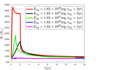
For the two cases with the RSG structure does not change much, and the RSG reaches a maximum radius of for S(46,0.0014,1) and for S(46,0.0014,1). We will not present the density and mass profiles for these cases as they are of less interest to us.
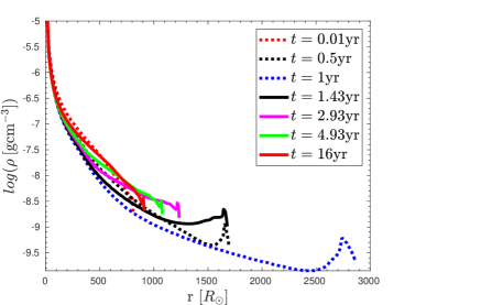
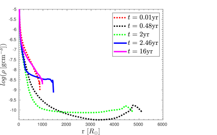
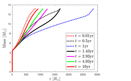
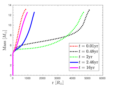
In Fig. 2 and 3 we present the density profiles at several times for simulations S(47,0.03,1) and S(48,0.59,2), respectively. In Figs. 4 and 5 we present the mass inner to radius as function of for several times of simulations S(47,0.03,1) and S(48,0.59,2), respectively. Because an energy injection phase of is much longer than the passage of the NS inside the RSG envelope, we will analyse in detail only the results of simulation S(47,0.03,1).
3.2 On the assumptions of the 1D models
Conducting the simulations with mesa implies two strong assumptions, that the star is spherically symmetric and that the stellar model is in hydrostatic equilibrium. Simply, the numerical code mesa (section 2) assumes a hydrostatic equilibrium of a spherically symmetric star. Neither of these two are correct for the present highly non-spherical flow that result from the strong jets that the NS launches into the envelope (Schreier et al., 2021).
Strictly speaking, our results are not consistent when the expansion timescale of the star is shorter than the dynamical timescale at the given radius. This is the case during the first when the stellar radius is larger than in simulation S(47,0.03,1) and for the first in simulation S(48,0.59,2). The dynamical time of the RSG is , where is the average density of the RSG (including the core). We can therefore trust the results of simulation S(47,0.03,1) from when the radius has contracted back to (see solid-black line in Figs. 2 and 4 at ). For simulation S(48,0.59,2) we see from Figs. 3 and 5 that about half a year after the end of the energy injection and mass removal (i.e., at ) the radius rapidly decreases to .
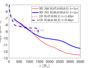
To show the qualitative agreement between the 1D and 3D simulations regarding the inflated envelope, we present in Fig. 6 the density profiles from the 1D simulations of models S(47,0.03,1) and S(48,0.59,2), with their respective equivalents from the 3D simulations of Schreier et al. (2021). All lines are at about half a year after the end of energy injection. For the 3D simulations this is at about , for S(47,0.03,1) it is at about , and for S(48,0.59,2) it is at about (see inset of Fig. 6 for the exact times).
Despite these limitations we do find that our simulations have merit and present new results.
Firstly, our 1D simulations validate the finding from the 3D simulations (Schreier et al., 2021) of an extended envelope to a radius of about twice the initial RSG radius, . The advantage of our simulations is that we do so with a full stellar code (for example, the 3D simulations did not include radiative transfer and convection). Since at these times the stellar zones had time to dynamically relax, we trust more the density profiles of our 1D simulations than those of the 3D simulations in these regions. The real densities at might be in between the profiles of the 1D and 3D simulations. Fig. 6 shows that the density of the inflated envelope out to has a large enough density to prolong the accretion phase of the NS, as we discuss in section 3.3.
Secondly, our simulations can follow the star for several years, unlike the 3D hydrodynamical-only simulations. We find that the star returns to almost its initial structure, but with less mass as we removed mass.
Let us comment on the thermal timescale. The energy that we deposit into the RSG not only drives the star out of dynamical equilibrium but also from thermal equilibrium. However, we first note that mesa is built to deal with stars out of thermal equilibrium, but still in hydrostatic equilibrium (e.g., section 2.3 in Paxton et al. 2015). For example, mesa calculates the pre-main sequence evolution that proceeds on a thermal time scale. Secondly, within the time that we consider the density profiles, at about half a year after the end of energy injection, the star radiates away its excess internal energy. We now show this.
At the relevant times of about half a year after the end of energy injection, for model S(47,0.03,1) and for model S(48,0.59,2), the required stellar luminosity to make the thermal timescale about equal to the simulation time is
| (1) |
where we substituted typical values at the relevant times. We find from our simulations that the luminosities are , , and for model S(47,0.03,1), and , , and for model S(48,0.59,2).
Considering the approximate nature of equation (1), we conclude that our inflated stellar model manages to arrange itself thermally by half a year after energy injection ends. This is similar to many other simulations with mesa, e.g., in the simulations of Renzo & Götberg (2021) where accretion drives the star out of thermal equilibrium but the mass-accreting star radiates away its excess internal energy.
3.3 Prolonged accretion
The time in our simulations corresponds to the time when the NS enters the RSG envelope. Namely, when it starts to accrete mass at a high rate and to launch energetic jets. The NS reaches periastron at . In their three-dimensional hydrodynamical simulations Schreier et al. (2021) assume that the jets accretion phase ends when the NS exits the original photosphere of the RSG, and launches jets for a time of . However, the density distribution in their simulations show that the jets accelerate gas outwards, such that the NS star continues to move inside a relatively dense gas for a much longer time. Their simulations, however, did not include the correct equation of stellar evolution. Our results here show that as the NS continues to move away from periastron and outside the original RSG envelope, it can accrete mass from a relatively dense envelope out to , about twice the original RSG radius. The trajectory of the NS brings it to at , i.e., about months after it left the original zone of the RSG envelope.
From the density profiles that we present in Fig. 2 we learn that the density at at is about , where is the initial RSG density at , the periastron distance of the NS. The velocity of the NS at periastron is , while it is about half this value at , . The Bondi-Hoyle-Lyttleton accretion rate by the NS goes as . From these values we find that the Bondi-Hoyle-Lyttleton accretion rate by the NS after it moves out from the initial location of the RSG photosphere and at about twice the original radius of the RSG is not much below that at periastron. Namely, for simulation S(47,0.03,1). Note that the actual accretion rate will be due to the negative jet feedback mechanism (e.g., Grichener, Cohen, & Soker 2021; Hillel et al. 2022).
4 Discussion and Summary
Using the one-dimensional stellar evolution code mesa (section 2) we simulated the response of RSG stellar models to injection of energy to the outer envelope and to mass removal. We list the values of the five cases in Fig. 1. We take these values from the three-dimensional hydrodynamical simulations of Schreier et al. (2021). They simulated CEJSN impostor events where a NS on a highly eccentric orbit enters the RSG envelope for about half a year and then exits, to return after an orbital period of . Because of numerical limitations we could not simulate the most energetic cases that Schreier et al. (2021) simulated. We therefore analysed in detail the simulation S(47,0.03,1) for which we present the density profiles and mass profiles for in Figs. 2 and 4, respectively.
From Fig. 1, 2 and 3 we see that the next time the NS enters the RSG envelope, about 16 years later, the RSG has relaxed to have more or less its original structure. The RGB has a little less mass, as we removed mass, and its radius is a little larger. But the CEJSN impostor event can repeat itself to have similar properties to the previous event.
Because of the assumption of hydrostatic equilibrium in the numerical procedure we cannot trust the stellar structure when the envelope is highly inflated at early times (section 3.1). We can trust the structure at later times after the envelope has contracted, like at when the RSG radius is about twice its initial radius (solid-black lines in Figs. 2 and 4).
Our main conclusion is that because the jets that the NS launches while inside the dense RSG envelope inflate an envelope with a non-negligible mass (Fig. 4 and 5), the NS continues to accrete at a relatively high rate to distances that are about twice the original RSG radius of (section 3.3). This means several more months of jet-activity. The accretion rate at these distances, of up to for simulation R(47,0.03,1), can be few tenths of the accretion rate at periastron passage of radius , i.e., .
Despite the fact that the jets that the NS launches while orbiting in the inflated envelope are much weaker than the jets that the NS launches inside the original RSG envelope zone, these late jets might actually be more influential on the light curve. Schreier et al. (2021) estimate that the efficiency of converting the jets’ energy to radiation increases from in the lowest energy simulation they perform with , to in their simulation with , and to in the simulation with . Most of the energy that these jets deposit to the envelope goes to perform work. As the gas expands it cools adiabatically, and therefore only a small fraction of the energy of these jets ends in radiation. The late jets that the NS launches while at larger orbital separations interact with the already ejected mass at large distances. This implies a longer expansion time and therefore the gas suffers only small adiabatic losses. In addition, the lower optical depth in the outer regions implies a shorter photon diffusion time to the photosphere, and therefore further allowing more thermal energy to be radiated away before the gas suffers adiabatic losses. Kaplan & Soker (2020) study the role of late jets on the light curve of core collapse supernovae and found that the efficiency of converting the energy of late jets to radiation can be up to .
In the simulations of Schreier et al. (2021) the periastron distance is , and they simulated cases with jets’ energies up to three orders of magnitude larger than in simulation S(47,0.03,1). According to the jet feedback mechanism results of Grichener, Cohen, & Soker (2021) and Hillel et al. (2022) we indeed expect that the jets’ energy in the simulations of Schreier et al. (2021) be two to three orders of magnitude larger than the jets’ energy in simulation S(47,0.03,1). The injected energy in simulation S(47,0.03,1) might correspond to a situation where the NS enters only the very outer region of the RSG envelope, and therefore the mass accretion rate is lower and therefore the jets’ power is lower, and spends only a short time there, only few weeks. Namely, for an orbit where the periastron distance is close to the surface, i.e., , where is the unperturbed radius of the RSG. Our results suggest that even in these cases the CEJSN impostor event will be bright because the NS will continue to launch jets as it orbits inside the inflated envelope for months after it has left the original zone of RSG envelope. The luminosity can be for the Bondi-Hoyle-Lyttleton accretion rate from the inflated envelope of that we estimated in section 3.3. Note that the actual accretion rate would be because of the negative jet feedback mechanism (e.g., Grichener, Cohen, & Soker 2021; Hillel et al. 2022). The peak duration might be several weeks.
On a broader scope, our study adds to the claim that CEJSN impostors might account for puzzling-rare transient events and to the rich variety of light curves that such jet-driven events have.
Acknowledgements
This research was supported by the Amnon Pazy Research Foundation. We thank an anonymous referee for pointing out the limitation of the mesa code.
Data availability
The data underlying this article will be shared on reasonable request to the corresponding author.
References
- Akashi & Soker (2021) Akashi M., Soker N., 2021, ApJ, 923, 55. doi:10.3847/1538-4357/ac2d2b
- Arcavi et al. (2017) Arcavi, I., Howell, D. A., Kasen, D., et al. 2017, Nature, 551, 210
- Armitage & Livio (2000) Armitage, P. J., & Livio, M. 2000, ApJ, 532, 540
- Baltay et al. (2013) Baltay, C., Rabinowitz, D., Hadjiyska, E., Walker, E. S., Nugent, P., Coppi, P., Ellman, N., et al. 2013, PASP, 125, 683. doi:10.1086/671198
- Bellm et al. (2019) Bellm, E. C., Kulkarni, S. R., Graham, M. J., Dekany, R., Smith, R. M., Riddle, R., Masci, F. J., et al. 2019, PASP, 131, 018002. doi:10.1088/1538-3873/aaecbe
- Chamandy et al. (2018) Chamandy, L., Frank, A., Blackman, E. G., et al. 2018, MNRAS, 480, 1898
- Chevalier (1993) Chevalier, R. A. 1993, ApJ, 411, L33
- Chevalier (2012) Chevalier, R. A. 2012, ApJ, 752, L2
- Dong et al. (2021) Dong D. Z., Hallinan G., Nakar E., Ho A. Y. Q., Hughes A. K., Hotokezaka K., Myers S. T., et al., 2021, Sci, 373, 1125. doi:10.1126/science.abg6037
- Fragos et al. (2019) Fragos, T., Andrews, J. J., Ramirez-Ruiz, E., Meynet, G., Kalogera, V., Taam, R. E., & Zezas, A., 2019, ApJ, 883, L45. doi:10.3847/2041-8213/ab40d1
- Fryer et al. (1996) Fryer, C. L., Benz, W., & Herant, M. 1996, ApJ, 460, 801
- Fryxell et al. (2000) Fryxell, B., et al. 2000, ApJS, 131, 273
- García et al. (2021) García, F., Simaz Bunzel, A., Chaty, S., Porter, E., & Chassande-Mottin, E. 2021, A&A, 649, A114. doi:10.1051/0004-6361/202038357
- Gilkis et al. (2019) Gilkis, A., Soker, N., & Kashi, A. 2019, MNRAS, 482, 4233
- Glanz & Perets (2021) Glanz, H. & Perets, H. B. 2021, MNRAS, 507, 2659. doi:10.1093/mnras/stab2291
- Grichener, Cohen, & Soker (2021) Grichener A., Cohen C., Soker N., 2021, ApJ, 922, 61. doi:10.3847/1538-4357/ac23dd
- Grichener, Kobayashi, & Soker (2022) Grichener A., Kobayashi C., Soker N., 2022, ApJL, 926, L9. doi:10.3847/2041-8213/ac4f68
- Grichener & Soker (2019a) Grichener, A., & Soker, N. 2019b, ApJ, 878, 24
- Grichener & Soker (2019b) Grichener, A. & Soker, N. 2019b, arXiv:1909.06328
- Grichener & Soker (2020) Grichener, A. & Soker, N. 2020, work presented at the EAS Annual Meeting (EWASS) 2020.
- Grichener & Soker (2021) Grichener, A. & Soker, N. 2021, MNRAS, 507, 1651. doi:10.1093/mnras/stab2233
- Hillel et al. (2022) Hillel, S., Schreier, R., & Soker, N. 2022, MNRAS, 514, 3212. doi:10.1093/mnras/stac1341
- Holgado et al. (2021) Holgado, A. M., Silva, H. O., Ricker, P. M., & Yunes, N., 2021, ApJ, 910, L22. doi:10.3847/2041-8213/abecdd
- Houck & Chevalier (1991) Houck, J. C., & Chevalier, R. A. 1991, ApJ, 376, 234
- Ivezić et al. (2019) Ivezić, Ž., Kahn, S. M., Tyson, J. A., Abel, B., Acosta, E., Allsman, R., Alonso, D., et al. 2019, ApJ, 873, 111. doi:10.3847/1538-4357/ab042c
- Kaplan & Soker (2020) Kaplan N., Soker N., 2020, MNRAS, 492, 3013. doi:10.1093/mnras/staa020
- Ko et al. (2022) Ko T., Tsuna D., Takei Y., Shigeyama T., 2022, ApJ, 930, 168. doi:10.3847/1538-4357/ac67e1
- Kochanek et al. (2017) Kochanek, C. S., Shappee, B. J., Stanek, K. Z., Holoien, T. W.-S., Thompson, T. A., Prieto, J. L., Dong S., et al. 2017, PASP, 129, 104502. doi:10.1088/1538-3873/aa80d9
- Livio et al. (1986) Livio, M., Soker, N., de Kool, M., & Savonije, G. J., 1986, MNRAS, 222, 235. doi:10.1093/mnras/222.2.235
- Lombardi et al. (2006) Lombardi, J. C., Jr., Proulx, Z. F., Dooley, K. L., Theriault, E. M., Ivanova, N., & Rasio, F. A. 2006, ApJ, 640, 441
- López-Cámara et al. (2019) López-Cámara, D., De Colle, F., & Moreno Méndez, E. 2019, MNRAS, 482, 3646
- López-Cámara et al. (2020) López-Cámara, D., Moreno Méndez, E., & De Colle, F. 2020, MNRAS, 497, 2057
- MacLeod & Ramirez-Ruiz (2015a) MacLeod, M., & Ramirez-Ruiz, E. 2015a, ApJ, 798, L19
- MacLeod et al. (2017) MacLeod, M., Antoni, A., Murguia-Berthier, A., Macias, P., & Ramirez-Ruiz, E. 2017, ApJ, 838, 56
- MacLeod & Ramirez-Ruiz (2015b) MacLeod, M., & Ramirez-Ruiz, E. 2015b, ApJ, 803, 41
- Mcley & Soker (2014) Mcley L., Soker N., 2014, MNRAS, 445, 2492. doi:10.1093/mnras/stu1952
- Moreno Méndez et al. (2017) Moreno Méndez, E., López-Cámara, D., & De Colle, F. 2017, MNRAS, 470, 2929
- Papish et al. (2015) Papish, O., Soker, N., & Bukay, I. 2015, MNRAS, 449, 288
- Paxton et al. (2011) Paxton, B., Bildsten, L., Dotter, A., et al. 2011, ApJS, 192, 3
- Paxton et al. (2013) Paxton, B., Cantiello, M., Arras, P., et al. 2013, ApJS, 208, 4
- Paxton et al. (2015) Paxton, B., Marchant, P., Schwab, J., et al. 2015, ApJS, 220, 15
- Paxton et al. (2018) Paxton, B., Schwab, J., Bauer, E. B., et al. 2018, ApJS, 234, 34
- Paxton et al. (2019) Paxton, B., Smolec, R., Schwab, J., et al. 2019, ApJS, 243, 10,
- Rasio & Shapiro (1991) Rasio, F. A., & Shapiro, S. L. 1991, ApJ, 377, 559
- Renzo & Götberg (2021) Renzo M., Götberg Y., 2021, ApJ, 923, 277. doi:10.3847/1538-4357/ac29c5
- Ricker & Taam (2008) Ricker, P. M., & Taam, R. E. 2008, ApJ, 672, L41
- Schreier et al. (2021) Schreier R., Hillel S., Shiber S., Soker N., 2021, MNRAS, 508, 2386. doi:10.1093/mnras/stab2687
- Schrøder et al. (2020) Schrøder, S. L., MacLeod, M., Loeb, A., et al. 2020, ApJ, 892, 13
- Shiber et al. (2019) Shiber, S., Iaconi, R., De Marco, O., & Soker, N. 2019, MNRAS, 488, 5615. doi:10.1093/mnras/stz2013
- Shiber et al. (2016) Shiber, S., Schreier, R., & Soker, N. 2016, RAA, 16, 117
- Soker (2016) Soker N., 2016, NewAR, 75, 1. doi:10.1016/j.newar.2016.08.002
- Soker (2021a) Soker, N. 2021a, ApJ, 906, 1. doi:10.3847/1538-4357/abca8f
- Soker (2021b) Soker, N. 2021b, MNRAS. doi:10.1093/mnras/stab1275
- Soker (2021c) Soker, N. 2021c, arXiv:2105.06452
- Soker (2022) Soker N., 2022, in preparation.
- Soker & Gilkis (2018) Soker, N., & Gilkis, A. 2018, MNRAS, 475, 1198
- Soker et al. (2019) Soker, N., Grichener, A., & Gilkis, A. 2019, MNRAS, 484, 4972
- Thöne et al. (2011) Thöne, C. C., de Ugarte Postigo, A., Fryer, C. L., Page, K. L., Gorosabel, J., Aloy, M. A., Perley, D. A., et al., 2011, Natur, 480, 72. doi:10.1038/nature10611
- Thorne & Zytkow (1977) Thorne K. S., Zytkow A. N., 1977, ApJ, 212, 832. doi:10.1086/155109
- Turk et al. (2011) Turk, M. J., Smith, B. D., Oishi, J. S., et al. 2011, ApJS, 192, 9
- Vick et al. (2021) Vick, M., MacLeod, M., Lai, D., & Loeb A. 2021, MNRAS, 503, 5569. doi:10.1093/mnras/stab850
- Yang et al. (2021) Yang S., Sollerman J., Chen T.-W., Kool E. C., Lunnan R., Schulze S., Strotjohann N., et al., 2021, A&A, 646, A22. doi:10.1051/0004-6361/202039440
- Zevin et al. (2021) Zevin, M., Bavera, S. S., Berry, C. P. L., et al. 2021, ApJ, 910, 152. doi:10.3847/1538-4357/abe40e
- Zheng & Yu (2021) Zheng, J.-H. & Yu, Y.-W. 2021, Research in Astronomy and Astrophysics, 21, 200. doi:10.1088/1674-4527/21/8/200