Static Replication of Impermanent Loss for Concentrated Liquidity Provision in Decentralised Markets

Abstract

This article analytically characterizes the impermanent loss of concentrated liquidity provision for automatic market makers in decentralised markets such as Uniswap. We propose two static replication formulas for the impermanent loss by a combination of European calls or puts with strike prices supported on the liquidity provision price interval. It facilitates liquidity providers to hedge impermanent loss by trading crypto options in more liquid centralised exchanges such as Deribit. Numerical examples illustrate the astonishing accuracy of the static replication.

[table]capposition=top

1 Introduction

Decentralised exchanges (DEXs) like Uniswap and Sushiswap facilitate traders to swap tokens in the listed liquidity pools by the architecture of automatic market making (AMM) without the intermediary centralised institutions. These exchanges utilize open-source protocols for providing liquidity and trading crypto tokens and all trades are recorded on Ethereum blockchain. The protocol is non-upgradable and designed to be censorship resistant without know-your-custom rule (KYC). Instead of using limited order book as in traditional centralised financial markets that would induce extreme costly gas fee by miners to verify transactions on blockchain, most DEXs such as Uniswap and Sushiswap use constant product function automated market making protocol. In this paper, we would treat the dominant decentralised exchange, Uniswap that initiates its first version protocol in November 2018. The Uniswap market lists over 400 tokens and 900 token pairs. The daily average trading volume exceeds 2 billion USD in 2022 where the most traded pair USDC/ETH consists of almost $50\%$ share of total volume, followed by USDT/ETH around 10% volume.

The constant product function automated market making protocol on Uniswap (see the v2 whitepaper Adams et al., [1]) allows traders to add, remove and swap tokens in the pool that could host any pair of tokens $(\mathtt{T_{X}},\mathtt{T_{Y}})$. The token $\mathtt{T_{Y}}$ (such as stablecoin USDC) is treated as the unit of account, i.e. the numeraire, and $\mathtt{T_{X}}$ is taken as the more volatile token such as ETH which is the native cryptocurrency on the Ethereum. For a pool with reserves $(X,Y)$ of tokens $(\mathtt{T_{X}},\mathtt{T_{Y}})$, to endogenously determine the pool price, the pool tracks the constant product ‘bonding’ reserve curve $X\cdot Y=L^{2}$. The constant $L$, called the liquidity, is set at the inception and remains unchanged across trades.

To exchange $\Delta X$ amount of token $\mathtt{T_{X}}$ for $\Delta Y$ quantity of token $\mathtt{T_{Y}}$, the trader must stay on the ‘bonding’ curve, i.e., $\left(X+\Delta X\right)\cdot\left(Y-\Delta Y\right)=L^{2}=XY.$ This means the trader could deposit $\Delta X$ number of token $\mathtt{T_{X}}$ to swap $\Delta Y=Y\cdot\Delta X/(X+\Delta X)$ token $\mathtt{T_{Y}}$ out from the pool. The product of new reserves $X^{{}^{\prime}}=X+\Delta X$ and $Y^{{}^{\prime}}=Y-\Delta Y$ remains the constant $X^{{}^{\prime}}\cdot Y^{{}^{\prime}}=L^{2}$. To compensate the risk, such as impermanent loss, taken by liquidity providers, the protocol would charge a swap fee $\gamma\cdot\Delta X$ in terms of token sending in. The fee rate $\gamma$ is initiated and unchangeable when the pool is created, e.g. $0.1\%,0.05\%,0.03\%$ and $0.01\%$ on Uniswap. The constant product ‘bonding’ curve endogenously yields a relative price in the pool. In this article, the pool price of token $\mathtt{T_{X}}$ is denominated in token $\mathtt{T_{Y}}$ as $P=Y/X$. In such a way, the reserves are $X=L/\sqrt{P}$ and $Y=L\sqrt{P}.$ A liquidity provider could add (remove) $\Delta L$ liquidity to the existing pool by depositing (redeeming) $\Delta X=\Delta L/\sqrt{P}$ number of token $\mathtt{T_{X}}$ and $\Delta Y=\Delta L\sqrt{P}$ of token $\mathtt{T_{Y}}$. The liquidity provision is supplied at the current price $P$ and does not alter the pool price.

The first and second protocol versions of Uniswap are criticized by low capital efficiency where liquidity provisions are dispersed on the price range $(0,\infty)$ and only a small fraction of total reserves is utilized during swap. Each liquidity provider only earns a small fraction fee proportional to her share in the pool. To promote capital efficiency through elimination of unused collateral, the Uniswap v3 protocol was launched on the Ethereum mainnet on May 2021 with the groundbreaking innovative feature of concentrated liquidity provision where liquidity providers could specify the price interval $[{\mathbb{P}}_{l},{\mathbb{P}}_{u}]$ that they are willing to supply liquidity, see the whitepaper Adams et al., [2]. This resembles limit order instead of market order in previous less-efficient v2 protocol. The ‘bonding’ curve is shifted as $\left(X+L/\sqrt{{\mathbb{P}}_{l}}\right)\cdot\left(Y+{L}{\sqrt{{\mathbb{P}}_{u}}}\right)=L^{2}.$ The details are given in the next section.

The liquidity provider is exposed to impermanent loss that is only realized until depleting liquidity and withdrawing the tokens from the pool. This loss is typically calculated as the difference of her supplied token pair value in the liquidity pool and the value of simply holding the tokens statically when entering the pool. Since traders always exchange less valuable token for more valuable one, liquidity providers always suffer impermanent loss (IL) that could be significant. Loesch et al., [14] estimate from May to Sep. 2021 the total IL is roughly $260.1 million USD and 49.5% of liquidity providers with negative returns in Uniswap v3 market.

In this paper, we propose a static hedge strategy for liquidity providers using standard European options to eliminate the impact of IL. First, we show that liquidity providers equivalently long and short different call and put options by liquidity provision and explicitly characterize the impermanent loss as a combination of several calls and puts with different strike prices and underlying driving processes. Second, we propose two static replication formulas that facilitate liquidity providers to hedge the impermanent loss risk by taking long positions of standard European call or put options in these centralised options market such as Deribit. At last, we numerically verify the static replication accuracy that would reduce liquidity providers’ impermanent loss risk tremendously.

We contribute to the continually growing body of literature on decentralised exchanges in several ways. For classical market making, we refer to the seminal works of [4], [17] and [12], to name a few. Angeris et al., [5] analyze no-arbitrage boundaries and price stability in Uniswap market. [15] show that the equilibrium utility in a decentralized market can be strictly higher than in a centralized market and Lehar and Parlour, [13] propose an equilibrium model and give conditions under which the automatic market making (AMM) dominates a limit order market and Capponi and Jia, [7] study the market microstructure of AMM. Another strand is to address the optimal liquidity provision in Uniswap market, see [6], [3] and [16]. However, they only focus on Uniswap v2 protocol either without the feature of concentrated liquidity provision or incorporating the impermanent loss. One exception is Loesch et al., [14] that empirically calculate the impermanent loss (IL) in Uniswap v3 market using the on-chain data. Our paper is more related to Clark, [10] that studies static replication in Uniswap v2 market. To the best of our knowledge, we are the first to characterize the option-like structure of IL that is both suffered from delta, vega and gamma exposures in Uniswap v3 market. Second, from methodological perspective, we propose a static option replication formula for squared-root price process that is further tailored to develop our replication formulas for the impermanent loss. It facilitates liquidity providers to hedge permanent loss by trading crypto options in more liquid centralised exchanges such as Deribit.

The rest of the paper is structured as follows. Section 2 introduces the concentrated liquidity provision protocol. In Section 3, we characterize the impermanent loss and present the static replication formulas. Section 4 demonstrates the static hedge replication accuracy and Section 5 concludes.

2 Concentrated Liquidity Provision

The constant product function protocol of Uniswap v2 facilitates token swapers and liquidity providers to interact with the pool automatically without any financial intermediaries, although suffering low capital efficiency. The Uniswap v3, launched on the Ethereum mainnet on May 2021, has popularized the innovative feature of concentrated liquidity provision. This increases the capital efficiency tremendously, up to 4000x relative to v2, at the sacrifice of higher leverage and impermanent loss.

When supplying liquidity, the liquidity provider specifies a lower price ${\mathbb{P}}_{l}$ and a upper price ${\mathbb{P}}_{u}$ and she earns transaction fees paid by swapers whenever the price remains in the interval $[{\mathbb{P}}_{l},{\mathbb{P}}_{u}]$. When the price moves out of the range $[{\mathbb{P}}_{l},{\mathbb{P}}_{u}]$, the position is inactive and she no longer earns any fee. Until the price re-enters into the interval, her position is activated again. Specifically, the ‘bonding’ curve of tokens $\mathtt{T_{X}}$ and $\mathtt{T_{Y}}$ satisfy the shifted constant product function

$$\left(X+L/\sqrt{{\mathbb{P}}_{l}}\right)\cdot\left(Y+{L}{\sqrt{{\mathbb{P}}_{u}}}\right)=L^{2}.$$ (1)

The amount $L/\sqrt{{\mathbb{P}}_{l}}$ and ${L}{\sqrt{{\mathbb{P}}_{u}}}$ are the virtual token reserves which are not tradable. Depending on the location of supported price interval $[{\mathbb{P}}_{l},{\mathbb{P}}_{u}]$ relative to the current price ${P_{0}}$, to supply $\Delta L$ liquidity, the liquidity provider’s deposits $\Delta X$ and $\Delta Y$ of tokens $\mathtt{T_{X}}$ and $\mathtt{T_{Y}}$ are

$$\Delta X =\left\{\begin{array}[]{cl}\Delta L\left(\frac{1}{\sqrt{{\mathbb{P}}_{l}}}-\frac{1}{\sqrt{{\mathbb{P}}_{u}}}\right),&\mbox{if}\quad P_{0}<{\mathbb{P}}_{l},\\ \Delta L\left(\frac{1}{\sqrt{P_{0}}}-\frac{1}{\sqrt{{\mathbb{P}}_{u}}}\right),&\mbox{if}\quad P_{0}\in[{\mathbb{P}}_{l},{\mathbb{P}}_{u}],\\ 0,&\mbox{if}\quad P_{0}>{\mathbb{P}}_{u}.\end{array}\right.$$ (5)

$$\Delta Y =\left\{\begin{array}[]{cl}0,&\mbox{if}\quad P_{0}<{\mathbb{P}}_{l},\\ \Delta L(\sqrt{P_{0}}-\sqrt{{\mathbb{P}}_{l}}),&\mbox{if}\quad P_{0}\in[{\mathbb{P}}_{l},{\mathbb{P}}_{u}],\\ \Delta L(\sqrt{{\mathbb{P}}_{u}}-\sqrt{{\mathbb{P}}_{l}}),&\mbox{if}\quad P_{0}>{\mathbb{P}}_{u}.\end{array}\right.$$ (9)

The deposits $\Delta X$ and $\Delta Y$ could be regarded as the trading volume that are needed to move price out the supported interval $[{\mathbb{P}}_{l},{\mathbb{P}}_{u}]$ from the lower boundary ${\mathbb{P}}_{l}$ and the upper boundary ${\mathbb{P}}_{u}$. The liquidity $\Delta L$ is not a tradable asset, only a synonym of token reserves $\Delta X$ and $\Delta Y$. Several important facts follows from (5).

1. The liquidity $\Delta L$ supplied on the interval $[{\mathbb{P}}_{l},{\mathbb{P}}_{u}]$ could be treated as uniformly distributed. We only illustrate one case when ${\mathbb{P}}_{l}\leq P_{0}\leq{\mathbb{P}}_{u}$, where $P_{0}$ is the current pool price. That means if we artificially split $[{\mathbb{P}}_{l},{\mathbb{P}}_{u}]$ into two sub-intervals $[{\mathbb{P}}_{l},P_{0}]$ and $[P_{0},{\mathbb{P}}_{u}]$, the liquidity on two intervals are both equal to $\Delta L$. By the supply equations in (5), we could reformulate it as

   $$\Delta X =\underbrace{0}_{\Delta X^{l}\ \text{deposit on}\ [{\mathbb{P}}_{l},P_{0}]}+\underbrace{\Delta L\left(\frac{1}{\sqrt{{P_{0}}}}-\frac{1}{\sqrt{{\mathbb{P}}_{u}}}\right)}_{\Delta X^{r}\ \text{deposit on}\ [P_{0},{\mathbb{P}}_{u}]},$$ (10)

   $$\Delta Y =\underbrace{\Delta L(\sqrt{P_{0}}-\sqrt{{\mathbb{P}}_{l}})}_{\Delta Y^{l}\ \text{deposit on}\ [{\mathbb{P}}_{l},P_{0}]}+\underbrace{0}_{\Delta Y^{r}\ \text{deposit on }\ [P_{0},{\mathbb{P}}_{u}]}.$$ (11)

   It clearly shows that the provider supplies liquidity $\Delta L$ on the left interval $[{\mathbb{P}}_{l},P_{0}]$ with reserves $(\Delta X^{l},\Delta Y^{l})$ and on the right interval $[P_{0},{\mathbb{P}}_{u}]$ with reserves $(\Delta X^{r},\Delta Y^{r})$ simultaneously.

2. The discussion above motivates us considering liquidity provision only from two sides of the current price $P_{0}$ that means we treat the liquidity provision on ${\mathbb{P}}_{l}\leq{P_{0}}\leq{\mathbb{P}}_{u}$ as two independent and disjoint price bins $[{\mathbb{P}}_{l},{P_{0}}]$ and $[{P_{0}},{\mathbb{P}}_{u}]$. In doing so, on the lower price bin $[{\mathbb{P}}_{l},{P_{0}}]$ she only supplies token $\mathtt{T_{Y}}$ with the amount of $\Delta L(\sqrt{{P_{0}}}-\sqrt{{\mathbb{P}}_{l}})$, in the meanwhile, she only deposits token $\mathtt{T_{X}}$ with the amount of $\Delta L\left(\frac{1}{\sqrt{{P_{0}}}}-\frac{1}{\sqrt{{\mathbb{P}}_{u}}}\right)$ in the upper price bin. The two price intervals $[{\mathbb{P}}_{l},{P_{0}}]$ and $[{P_{0}},{\mathbb{P}}_{u}]$ resembles the bid-ask prices of the traditional limit-order-book. This would greatly simply the analysis of impermanent loss below.

3 Impermanent Loss of Liquidity Provision

The impermanent loss is the possible loss from liquidity provision, compared to the static strategy where the liquidity provider holds the corresponding tokens in the pool unchanged. Due to the change of token pool price, once the provider closes her position and exits the pool, the impermanent loss would be realized. Following [3], [11], and [14], we define the impermanent loss (IL) as follows.

Definition 3.1.

For a liquidity provision with deposits $X_{0}$ and $Y_{0}$ of tokens $\mathtt{T_{X}}$ and $\mathtt{T_{Y}}$ at initial time $0$, the realized impermanent loss (IL) at time $t$ when removing the liquidity is the capital loss if she holds token pair statically at initial time $0$ instead. Specifically, the impermanent loss (IL) is calculated as

$$\text{IL}=Y_{t}-Y_{0}+(X_{t}-X_{0})\cdot P_{t}.$$ (12)

Here, $X_{t}$ and $Y_{t}$ are the quantities withdrawn at time $t$ and $P_{t}$ is the price of token $\mathtt{T_{X}}$.

The impermanent loss is not defined as the difference between ‘exit’ value and ‘entry’ value as usual. Here, we take the same perspective of [3], [11], and [14] and industry practice that liquidity providers treat impermanent loss as the cost of buying their initial liquidity deposits back when exiting the pool. A recent work on other form of arbitrage and losses in decentralised exchanges (the so-called miner extractable value) is studied in Capponi et al., [8]. Since token $\mathtt{T_{Y}}$ is usual some stable-coin (such as USDC and USDT) with value pegged to 1 USD, we always consider the realized impermanent loss (IL) in terms of token $\mathtt{T_{Y}}$.

From the analysis in Section 2, we could treat each liquidity provision separately from two sides of the current pool price ${P_{0}}$. Without loss of generality, we assume the liquidity $\Delta L$ is supplied on the right side price interval $[{\mathbb{P}}_{l},{\mathbb{P}}_{u}]$ where ${P_{0}}\leq{\mathbb{P}}_{l}\leq{\mathbb{P}}_{u}$ that resembles the ask prices in limit order book. From (5), the number of tokens required to establish the position is

$$\Delta Y_{0}=0,\qquad\Delta X_{0}=\Delta L\left(\frac{1}{\sqrt{{\mathbb{P}}_{l}}}-\frac{1}{\sqrt{{\mathbb{P}}_{u}}}\right).$$ (13)

Now, we track the token holdings when the provider closes her position where the price changes from ${P_{0}}$ to $P_{t}$ at exiting time $t$. We distinguish three possible locations of price $P_{t}$.

1. $P_{t}\in[{\mathbb{P}}_{l},{\mathbb{P}}_{u}]:$ When the price increases and moves into the price interval $[{\mathbb{P}}_{l},{\mathbb{P}}_{u}]$, the initial reserve $\Delta X_{0}$ is partially converted to less valuable token $\mathtt{T_{Y}}$ that would induce loss to the liquidity provider. At time $t$, when exiting, the quantities of tokens $\mathtt{T_{Y}}$ and $\mathtt{T_{X}}$ can be retrieved from the pool are

   $$\Delta Y_{t}=\Delta L(\sqrt{P_{t}}-\sqrt{{\mathbb{P}}_{l}}),\quad\Delta X_{t}=\Delta L\left(\frac{1}{\sqrt{P_{t}}}-\frac{1}{\sqrt{{\mathbb{P}}_{u}}}\right).$$ (14)

   The amount of $\Delta X_{0}-\Delta X_{t}$ of token $\mathtt{T_{X}}$ is converted to token $\mathtt{T_{Y}}$ that would have been sell more if she does not provide liquidity. Therefore, the IL denominated in token $\mathtt{T_{Y}}$ is

   $$\text{IL}^{(1)} =\Delta L(\sqrt{P_{t}}-\sqrt{{\mathbb{P}}_{l}})+\Delta L\left(\frac{1}{\sqrt{P_{t}}}-\frac{1}{\sqrt{{\mathbb{P}}_{l}}}\right)P_{t}$$ (15)

   $$=\Delta L\left(2\sqrt{P_{t}}-\frac{P_{t}}{\sqrt{{\mathbb{P}}_{l}}}-\sqrt{{\mathbb{P}}_{l}}\right)\leq 0.$$ (16)

   With the escalating of token $\mathtt{T_{X}}$’s price, the provider is consistently and gradually selling more valuable token $\mathtt{T_{X}}$ for token $\mathtt{T_{Y}}$. Therefore, she suffers a loss.

2. $P_{t}\geq{\mathbb{P}}_{u}:$ When the price crosses above the upper price ${\mathbb{P}}_{u}$, all token reserve $\Delta X_{0}$ are converted to token $\mathtt{T_{Y}}$. The amount of tokens $\mathtt{T_{Y}}$ and $\mathtt{T_{X}}$ can be retrieved from the pool at time $t$ are

   $$\Delta Y_{t}=\Delta L(\sqrt{{\mathbb{P}}_{u}}-\sqrt{{\mathbb{P}}_{l}}),\quad\Delta X_{t}=0.$$ (17)

   Therefore, the IL is

   $$\text{IL}^{(2)} =\Delta L\left(\sqrt{{\mathbb{P}}_{u}}-\sqrt{{\mathbb{P}}_{l}}-\left(\frac{1}{\sqrt{{\mathbb{P}}_{l}}}-\frac{1}{\sqrt{{\mathbb{P}}_{u}}}\right){P_{t}}\right)\leq 0$$ (18)

   In the meanwhile, the average selling price of token $\mathtt{T_{X}}$ is $\Delta Y_{t}/\Delta X_{0}=\sqrt{{\mathbb{P}}_{u}{\mathbb{P}}_{l}}$, lower than the market price $P_{t}$.

3. $P_{t}\leq{\mathbb{P}}_{l}:$ When the price stays below the lower boundary ${\mathbb{P}}_{l}$, the quantity of token $\mathtt{T_{X}}$ is unchanged and the IL is 0.

Taking together, the aggregated impermanent loss from the right side price interval $\text{IL}^{\mathtt{R}}$ is

$$\frac{\text{IL}^{\mathtt{R}}}{\Delta L} =\left(2\sqrt{P_{t}}-\frac{P_{t}}{\sqrt{{\mathbb{P}}_{l}}}-\sqrt{{\mathbb{P}}_{l}}\right)\mathds{1}_{\{{\mathbb{P}}_{l}\leq P_{t}\leq{\mathbb{P}}_{u}\}}$$ (19)

$$+\left(\sqrt{{\mathbb{P}}_{u}}-\sqrt{{\mathbb{P}}_{l}}-\left(\frac{1}{\sqrt{{\mathbb{P}}_{l}}}-\frac{1}{\sqrt{{\mathbb{P}}_{u}}}\right){P_{t}}\right)\mathds{1}_{\{P_{t}\geq{\mathbb{P}}_{u}\}}.$$ (20)

Similar argument to the liquidity provision from the left side price interval $[\mathbb{S}_{l},\mathbb{S}_{u}]$ (i.e. $\mathbb{S}_{l}\leq\mathbb{S}_{u}\leq P_{0}$) leads to

$$\frac{\text{IL}^{\mathtt{L}}}{\Delta L} =\left(2\sqrt{P_{t}}-\frac{P_{t}}{\sqrt{{\mathbb{S}}_{u}}}-\sqrt{{\mathbb{S}}_{u}}\right)\mathds{1}_{\{{\mathbb{S}}_{l}\leq P_{t}\leq{\mathbb{S}}_{u}\}}$$ (21)

$$+\left(\left(\frac{1}{\sqrt{{\mathbb{S}}_{l}}}-\frac{1}{\sqrt{{\mathbb{S}}_{u}}}\right){P_{t}}-\sqrt{{\mathbb{S}}_{u}}+\sqrt{{\mathbb{S}}_{l}}\right)\mathds{1}_{\{P_{t}\leq{\mathbb{S}}_{l}\}}.$$ (22)

We call the ratio $\text{IL}/\Delta L$ as unit impermanent loss per liquidity (UIL). Rearranging (19) and (21) gives the following representation.

Proposition 3.2.

The impermanent loss per liquidity (UIL) is characterized as a combination of short and long positions in different call options as following.

$$\rm{UIL}^{\mathtt{R}} =2\left(\sqrt{P_{t}}-\sqrt{{\mathbb{P}}_{l}}\right)^{+}-2\left(\sqrt{P_{t}}-\sqrt{{\mathbb{P}}_{u}}\right)^{+}$$ (23)

$$-\frac{1}{\sqrt{{\mathbb{P}}_{l}}}\left({P_{t}}-{{\mathbb{P}}_{l}}\right)^{+}+\frac{1}{\sqrt{{\mathbb{P}}_{u}}}\left({P_{t}}-{{\mathbb{P}}_{u}}\right)^{+},$$ (24)

$$\rm{UIL}^{\mathtt{L}} =2\left(\sqrt{{\mathbb{S}}_{l}}-\sqrt{P_{t}}\right)^{+}-2\left(\sqrt{{\mathbb{S}}_{u}}-\sqrt{P_{t}}\right)^{+}$$ (25)

$$-\frac{1}{\sqrt{{\mathbb{S}}_{l}}}\left({{\mathbb{S}}_{l}}-{P_{t}}\right)^{+}+\frac{1}{\sqrt{{\mathbb{S}}_{u}}}\left({{\mathbb{S}}_{u}}-{P_{t}}\right)^{+}.$$ (26)

Proposition 3.2 demonstrates the unit impermanent loss $\text{UIL}^{\mathtt{R}}$ ($\text{UIL}^{\mathtt{L}}$) is equivalent to hold two types of long call (put) options with price process $P_{t}$ and squared root price process $\sqrt{P_{t}}$ and also two short call (put) positions. The strike prices are either the lower boundary $\mathbb{P}_{l}$ or the upper boundary $\mathbb{P}_{u}$. This also means liquidity providers suffer all standard European option’s risk such as vega and gamma exposures.

Assuming risk-free rate is zero and $P_{t}$ obeys geometric Brownian motion, we have the following corollary.

Corollary 3.3.

If the price $P_{t}$ of token $\mathtt{T_{X}}$ is driven by a geometric Brownian motion with volatility $\sigma$, the impermanent loss per liquidity $\text{UIL}^{\mathtt{R}}$ and $\text{UIL}^{\mathtt{L}}$ are

$${\mathbb{E}[\rm{UIL}^{\mathtt{R}}]} =2\sqrt{P_{0}}\exp\left({-\frac{\sigma^{2}t}{8}}\right)\left(N(d_{l}+\sigma\sqrt{t}/2)-N(d_{u}+\sigma\sqrt{t}/2)\right)$$ (27)

$$-\sqrt{\mathbb{P}_{l}}N(d_{l})+\sqrt{\mathbb{P}_{u}}N(d_{u})$$ (28)

$$-\frac{1}{\sqrt{{\mathbb{P}}_{l}}}P_{0}N(d_{l}+\sigma\sqrt{t})+\frac{1}{\sqrt{{\mathbb{P}}_{u}}}P_{0}N(d_{u}+\sigma\sqrt{t}),$$ (29)

$${\mathbb{E}[\rm{UIL}^{\mathtt{L}}]} =2\sqrt{P_{0}}\exp\left({-\frac{\sigma^{2}t}{8}}\right)\left(-N(-q_{l}-\sigma\sqrt{t}/2)\right.$$ (30)

$$\left.+N(-q_{u}-\sigma\sqrt{t}/2)\right)+\sqrt{\mathbb{S}_{l}}N(-q_{l})-\sqrt{\mathbb{S}_{u}}N(-q_{u})$$ (31)

$$+\frac{1}{\sqrt{{\mathbb{S}}_{l}}}P_{0}N(-q_{l}-\sigma\sqrt{t})-\frac{1}{\sqrt{{\mathbb{S}}_{u}}}P_{0}N(-q_{u}-\sigma\sqrt{t}).$$ (32)

Here, $N(\cdot)$ is the standard normal cumulative distribution function and

$$d_{u} =\frac{\ln(P_{0}/{\mathbb{P}}_{u})-\sigma^{2}t/2}{\sigma\sqrt{t}},\quad d_{l}=\frac{\ln({P_{0}}/{\mathbb{P}}_{l})-\sigma^{2}t/2}{\sigma\sqrt{t}},$$ (33)

$$q_{u} =\frac{\ln(P_{0}/{\mathbb{S}}_{u})-\sigma^{2}t/2}{\sigma\sqrt{t}},\quad q_{l}=\frac{\ln({P_{0}}/{\mathbb{S}}_{l})-\sigma^{2}t/2}{\sigma\sqrt{t}}.$$ (34)

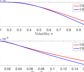
Figure 1: Impermanent Loss Sensitives

Note. Here, we set $\Delta L=1,\ \sigma=0.7$. The initial pool price is $P_{0}=10$ and the liquidity provider supplies on the upper price interval $[{\mathbb{P}}_{l},{\mathbb{P}}_{u}]=[11,12]$ and lower price interval $[{\mathbb{S}}_{l},{\mathbb{S}}_{u}]=[8,9]$ and closes her position after one month, i.e. $t=30$ days.

Figure 1 shows the impermanent loss ${\mathbb{E}[\text{UIL}^{\mathtt{R}}]}$ and ${\mathbb{E}[\text{UIL}^{\mathtt{L}}]}$ are both declining with the increasing of volatility and exiting time $t$. It all shows the asymmetric pattern that the right side liquidity provision ${\mathbb{E}[\text{UIL}^{\mathtt{R}}]}$ is less sensitive to vega and theta risk.

3.1 Static Replication of Impermanent Loss

Proposition 3.2 demonstrates the impermanent loss is an “option-like” instrument that can not be easily hedged by underlying asset and futures. In this section, we statically replicate (or hedge) the impermanent loss by standard European call or put options. Here, static replication means the liquidity provider could buy a combination of calls or puts at inception and hold the position statically until removing her liquidity from the pool. This lowers transaction and re-balancing cost for them. We start with two basic equalities.

Lemma 3.4.

The following two equations hold.

$$\left(\sqrt{x}-\sqrt{\widehat{K}}\right)^{+} =\frac{\widehat{K}^{-\frac{1}{2}}}{2}\left(x-\widehat{K}\right)^{+}-\frac{1}{4}\int_{\widehat{K}}^{\infty}K^{-\frac{3}{2}}\left(x-K\right)^{+}\mathrm{d}K,\$$ (35)

$$\left(\sqrt{\widehat{K}}-\sqrt{x}\right)^{+} =\frac{\widehat{K}^{-\frac{1}{2}}}{2}\left(\widehat{K}-x\right)^{+}+\frac{1}{4}\int_{0}^{\widehat{K}}K^{-\frac{3}{2}}\left(K-x\right)^{+}\mathrm{d}K.$$ (36)

Proof.

Any twice differentiable function $f$ can be represented as (see Carr and Madan, [9])

$$f(x) =f(x^{\star})+f^{{}^{\prime}}(x^{\star})(x-x^{\star})$$ (37)

$$+\int_{0}^{x^{\star}}f^{{}^{\prime\prime}}(K)(K-x)^{+}\mathrm{d}K+\int_{x^{\star}}^{+\infty}f^{{}^{\prime\prime}}(K)(x-K)^{+}\mathrm{d}K.$$ (38)

Applying formula (37) to $f(x)=\sqrt{x}-\sqrt{\widehat{K}}$ and choose $x^{\star}=\widehat{K}$, we have

$$\sqrt{x}-\sqrt{\widehat{K}} =\frac{1}{2}\widehat{K}^{-\frac{1}{2}}\left(x-\widehat{K}\right)-\frac{1}{4}\int_{0}^{\widehat{K}}K^{-\frac{3}{2}}\left(K-x\right)^{+}\mathrm{d}K$$ (39)

$$-\frac{1}{4}\int_{\widehat{K}}^{+\infty}K^{-\frac{3}{2}}\left(x-K\right)^{+}\mathrm{d}K.$$ (40)

Multiplying $\mathds{1}_{\{x\geq\widehat{K}\}}$ in the above equation, it yields (35). Similar argument leads to (36). This completes the proof. ∎

Proposition 3.5.

The impermanent loss per liquidity (UIL) can be statically replicated by

$$\mathbb{E}[{\rm{UIL}}^{\mathtt{R}}] =-\frac{1}{2}\int_{{\mathbb{P}}_{l}}^{{\mathbb{P}}_{u}}K^{-\frac{3}{2}}{\mathbf{C}}(K)\mathrm{d}K,$$ (41)

$$\mathbb{E}[{\rm{UIL}}^{\mathtt{L}}] =-\frac{1}{2}\int_{{\mathbb{S}}_{l}}^{{\mathbb{S}}_{u}}K^{-\frac{3}{2}}\mathbf{P}(K)\mathrm{d}K.$$ (42)

Here, $\mathbf{C}(K)$ and $\mathbf{P}(K)$ are European call and put option prices with maturity $t$ and strike price $K$.

Especially, when the provider supplies liquidity over $(0,\infty)$ as in Uniswap v2, the total UIL is $-\frac{1}{2}\int_{P_{0}}^{\infty}K^{-\frac{3}{2}}{\mathbf{C}}(K)\mathrm{d}K-\frac{1}{2}\int_{0}^{P_{0}}K^{-\frac{3}{2}}\mathbf{P}(K)\mathrm{d}K$.

Proof.

Using equations (35) and (23) of Lemma 3.4 and Proposition 3.2 with $x=P_{t}$ and $\widehat{K}\in\{{\mathbb{P}}_{l},{\mathbb{P}}_{u}\}$, we have

$$\text{UIL}^{\mathtt{R}} =2\left(\sqrt{P_{t}}-\sqrt{{\mathbb{P}}_{l}}\right)^{+}-2\left(\sqrt{P_{t}}-\sqrt{{\mathbb{P}}_{u}}\right)^{+}$$ (43)

$$-\frac{1}{\sqrt{{\mathbb{P}}_{l}}}\left({P_{t}}-{{\mathbb{P}}_{l}}\right)^{+}+\frac{1}{\sqrt{{\mathbb{P}}_{u}}}\left({P_{t}}-{{\mathbb{P}}_{u}}\right)^{+}$$ (44)

$$={\mathbb{P}}_{l}^{-\frac{1}{2}}\left(P_{t}-{\mathbb{P}}_{l}\right)^{+}-\frac{1}{2}\int_{{\mathbb{P}}_{l}}^{+\infty}K^{-\frac{3}{2}}\left(P_{t}-K\right)^{+}\mathrm{d}K$$ (45)

$$-{\mathbb{P}}_{u}^{-\frac{1}{2}}\left(P_{t}-{\mathbb{P}}_{u}\right)^{+}+\frac{1}{2}\int_{{\mathbb{P}}_{u}}^{+\infty}K^{-\frac{3}{2}}\left(P_{t}-K\right)^{+}\mathrm{d}K$$ (46)

$$-{\mathbb{P}}_{l}^{-\frac{1}{2}}\left(P_{t}-{\mathbb{P}}_{l}\right)^{+}+{\mathbb{P}}_{u}^{-\frac{1}{2}}\left(P_{t}-{\mathbb{P}}_{u}\right)^{+}$$ (47)

$$=-\frac{1}{2}\int_{{\mathbb{P}}_{l}}^{{\mathbb{P}}_{u}}K^{-\frac{3}{2}}\left(P_{t}-K\right)^{+}\mathrm{d}K.$$ (48)

Taking expectation under risk-neutral probability gives the first equation in (41). Similar argument with (26) and (36) gives the second equality in (42). When the provider supplies liquidity over $(0,\infty)$ as in Uniswap v2, the supported price intervals are $[{\mathbb{P}}_{l},{\mathbb{P}}_{u}]=[P_{0},+\infty]$ and $[{\mathbb{S}}_{l},{\mathbb{S}}_{u}]=[0,P_{0}]$. This completes the proof. ∎

First of all, Proposition 3.5 shows the impermanent loss could be perfectly replicated via a group of call or put options with strike prices supported in the liquidity provision interval. This equips liquidity providers the vehicle to hedge the IL by trading options in the more liquid centralised cyptocurrency market such as Deribit. Second, the impermanent losses inherit all option Greeks such as delta, gamma and vega risk factors. For instance, the delta $\partial\mathbb{E}[{\rm{UIL}}^{\mathtt{R}}]/\partial P=-\frac{1}{2}\int_{{\mathbb{P}}_{l}}^{{\mathbb{P}}_{u}}K^{-\frac{3}{2}}\Delta_{\mathbf{C}}(K)\mathrm{d}K$ and $\Delta_{\mathbf{C}}(K)$ is the call option’s delta at strike price $K$. Third, in practice, only limited option strikes are traded in the market. Therefore, we use a discrete version of formulae (41) and (42), i.e. $\mathbb{E}[{\rm{UIL}}^{\mathtt{R}}]\simeq-0.5\sum_{i}K_{i}^{-3/2}\mathbf{C}(K_{i})\Delta K_{i}$ and $\mathbb{E}[{\rm{UIL}}^{\mathtt{L}}]\simeq-0.5\sum_{i}M_{i}^{-3/2}\mathbf{P}(M_{i})\Delta M_{i}.$ Here, $(K_{i})$ and $(M_{i})$ are the partitions of intervals $[{\mathbb{P}}_{u},\ {\mathbb{P}}_{l}]$ and $[{\mathbb{S}}_{u},\ {\mathbb{S}}_{l}]$ accordingly. The approximation would induce discretization errors for the replications which is evaluated in the following section.

4 Numerical Analysis

4.1 Discretization Errors

In this section, we assume the pool price is driven by the Heston process

$$\mathrm{d}P_{t} =\mu P_{t}\mathrm{d}t+\sqrt{\nu_{t}}P_{t}\mathrm{d}W^{P}_{t},\quad\mathrm{d}\nu_{t}=\kappa(\theta-\nu_{t})\mathrm{d}t+\xi\sqrt{\nu_{t}}\mathrm{d}W^{\nu}_{t}.$$ (49)

Here, $W^{P}$ and $W^{\nu}$ are two correlated Brownian motions with correlation $\rho$. In the numerical analysis, we assume the initial pool price $P_{0}=10$ and volatility $\nu_{0}=0.3$ and set $\mu=0.1$ and $\rho=-0.3$. The mean-reversion speed, volatility level and volatility-of-volatility are set as $\kappa=0.4,\theta=0.4$ and $\xi=0.15$ accordingly. The liquidity provider supplies liquidity in the upper price interval $[{\mathbb{P}}_{l},{\mathbb{P}}_{u}]=[11,14]$ and lower price interval $[{\mathbb{S}}_{l},{\mathbb{S}}_{u}]=[6,9]$ and closes her position after one week, i.e. $t=7$ days.

First, we use Monte Carlo method to estimate $\mathbb{E}[{\rm{UIL}}^{\mathtt{R}}],\ \mathbb{E}[{\rm{UIL}}^{\mathtt{L}}]$ and call and put prices. Second, the simple trapezoidal numerical integration is utilized to approximate the integrals in (41) and (42) with 100 different strikes in the intervals $[{\mathbb{P}}_{l},{\mathbb{P}}_{u}]$ and $[{\mathbb{S}}_{l},{\mathbb{S}}_{u}]$. Table 1 reports the replication error ratios. It shows in all scenarios the replication formulas yield highly accurate approximations for both right and left side impermanent losses if there are enough traded option strikes. The error ratios are roughly 0.1 base point (0.01%) for right side impermanent losses and 0.01bp for the left one. With the increasing of volatility level $\theta$, it also increases impermanent losses $\mathbb{E}[{\rm{UIL}}^{\mathtt{R}}]$ and $\mathbb{E}[{\rm{UIL}}^{\mathtt{L}}]$ simultaneously. The effects of reversion speed $\kappa$ and volatility-of-volatility $\xi$ are mixed.

Table 1: Static Replication Accuracy for Impermanent Loss per Liquidity

	$\mathbb{E}[\text{UIL}^{\mathtt{R}}]$	$\text{UIL}^{\mathtt{R}}$ Replication	Error Ratio
$\kappa=0.3$	-0.424263	-0.424267	1.03E-05
$\kappa=0.4$	-0.420756	-0.420761	1.03E-05
$\kappa=0.5$	-0.439243	-0.439248	1.02E-05
$\theta=0.3$	-0.411396	-0.411401	1.08E-05
$\theta=0.4$	-0.460699	-0.460703	1.01E-05
$\theta=0.5$	-0.501689	-0.501694	9.68E-06
$\xi=0.1$	-0.440122	-0.440126	1.02E-05
$\xi=0.15$	-0.497540	-0.497545	9.97E-06
$\xi=0.2$	-0.467309	-0.467313	1.02E-05
	$\mathbb{E}[\text{UIL}^{\mathtt{L}}]$	$\text{UIL}^{\mathtt{L}}$ Replication	Error Ratio
$\kappa=0.3$	-0.177913	-0.177913	1.59E-06
$\kappa=0.4$	-0.186653	-0.186652	1.83E-06
$\kappa=0.5$	-0.192570	-0.192570	1.41E-06
$\theta=0.3$	-0.150062	-0.150061	1.91E-06
$\theta=0.4$	-0.185478	-0.185477	1.58E-06
$\theta=0.5$	-0.217112	-0.217112	7.72E-07
$\xi=0.1$	-0.187169	-0.187168	1.72E-06
$\xi=0.15$	-0.182929	-0.182929	1.36E-06
$\xi=0.2$	-0.184267	-0.184267	1.18E-06

Note. The initial pool price and volatility are $P_{0}=10$ and $\nu_{0}=0.3$. Choose $\mu=0.1$ and $\rho=-0.3$. The mean-reversion speed, volatility level and volatility-of-volatility are set as $\kappa=0.4,\theta=0.4$ and $\xi=0.15$. The liquidity provider supplies liquidity in the upper price interval $[{\mathbb{P}}_{l},{\mathbb{P}}_{u}]=[11,14]$ and lower price interval $[{\mathbb{S}}_{l},{\mathbb{S}}_{u}]=[6,9]$ and closes her position after one month, i.e. $t=7$ days.

4.2 Replication Error on Deribit Option Market

In this section, we verify the replication accuracy using bitcoin options traded on Deribit exchange from 1, Jan. 2020 to 31, Dec. 2020. We access the tick-by-tick options data through Deribit API (application programming interface) which consists of 1,316,050 trades with the annual total volume of 56.7 billion USD.

On each day, we suppose the liquidity provider could randomly enter the Uniswap market and provide liquidity for the BTC-USDC pool from the right and left sides of current price, i.e., $[P_{0},u\cdot P_{0}]$ and $[d\cdot P_{0},P_{0}]$ and deplete liquidity until time $T$ (1 or 2 weeks). Here, $P_{0}$ is the entry bitcoin price and two constants $u>1$ and $d<1$ control the liquidity provision price intervals. The impermanent loss when exiting is calculated through equations (23) and (26).

In the meanwhile, the liquidity provider also longs a combination of calls (or puts) with strikes in $[P_{0},u\cdot P_{0}]$ (or $[d\cdot P_{0},P_{0}]$) and holds statically to maturity $T$. The call and put options gain are calculated via the means of

$$-0.5\sum_{i}K_{i}^{-3/2}(P_{T}-K_{i})^{+}\Delta K_{i},\quad\mbox{and},$$ (50)

$$-0.5\sum_{i}M_{i}^{-3/2}(M_{i}-P_{T})^{+}\Delta M_{i}.$$ (51)

Here, $P_{T}$ is the bitcoin price at time $T$ and $K_{i},M_{i}$ are all traded option strikes.

Table 2 shows several interesting facts: (1) the impermanent losses $\rm{UIL}^{\mathtt{R}}$ and $\rm{UIL}^{\mathtt{L}}$ both increase with more wider liquidity provision intervals (larger $u$ and smaller $d$); (2) the right side loss $\rm{UIL}^{\mathtt{R}}$ is more severe than left side loss $\rm{UIL}^{\mathtt{L}}$. The intuition is the bitcoin price soars from 4,000 to nearly 30,000 in 2020 and right side liquidity provision would be much more risky; (3) even-though only a few strikes (3, 7, 10) are traded, the replication errors are reasonable, especially for this particular volatile markets; (4) we do not observe obvious patterns when the liquidity provision duration is longer.

Table 2: Static Replication using Deribit Option

T(week)	Price Interval	$\mathbb{E}[\text{UIL}^{\mathtt{R}}]$	Static	#Strikes
1	$u=1.1$	-1.588	-0.991	3
	$u=1.2$	-2.735	-2.294	7
	$u=1.3$	-3.597	-3.253	10
2	$u=1.1$	-1.586	-0.921	3
	$u=1.2$	-2.726	-2.216	7
	$u=1.3$	-3.569	-3.157	10
		$\mathbb{E}[\text{UIL}^{\mathtt{L}}]$	Static	#Strikes
1	$d=0.9$	-0.097	-0.066	3
	$d=0.8$	-0.154	-0.122	7
	$d=0.7$	-0.182	-0.149	10
2	$d=0.9$	-0.101	-0.068	3
	$d=0.8$	-0.158	-0.124	7
	$d=0.7$	-0.187	-0.154	10

Note. The liquidity provider provides liquidity for the BTC-USDC pool from the right and left sides of current price, i.e., $[P_{0},u\cdot P_{0}]$ and $[d\cdot P_{0},P_{0}]$ and deplete liquidity until time $T$ (1 or 2 weeks). The two constants $u>1$ and $d<1$ control the liquidity provision price intervals. In the meanwhile, the liquidity provider also trades Deribit bitcoin options via the static replication formulae (41) and (42), reported in column “static”. The column “#Strikes” is the average number of traded option strikes in the provision price intervals.

5 Conclusion

Liquidity providers supply crypto tokens from the right and left sides of the current price in decentralised markets such as Uniswap where they are exposed to impermanent loss. We analytically characterize the option-like payoff structures of impermanent losses for concentrated liquidity provision and propose two static replication formulas for the impermanent loss by a combination of European calls or puts with strike prices supported on the liquidity provision price interval. Liquidity providers could hedge their permanent loss by trading options in more liquid centralised exchanges such as Deribit. The Heston stochastic diffusion model illustrates the extreme accuracy of replication formulas when there are enough traded option strikes. Further evidences from Deribit bitcoin option market confirm the usefulness and accuracy of the static replication formulae.

References

References

- Adams et al., [2020] Adams, H., Zinsmeister, N., and Robinson, D. (2020). Uniswap v2 core. https://uniswap.org/whitepaper.pdf.
- Adams et al., [2021] Adams, H., Zinsmeister, N., Salem, M., Keefer, R., and Robinson, D. (2021). Uniswap v3 core. Thttps://startcy.io/whitepaper-v3.pdf.
- Aigner and Dhaliwal, [2021] Aigner, A. A. and Dhaliwal, G. (2021). Uniswap: Impermanent loss and risk profile of a liquidity provider. arXiv preprint arXiv:2106.14404.
- Amihud and Mendelson, [1980] Amihud, Y. and Mendelson, H. (1980). Dealership market: Market-making with inventory. Journal of financial economics, 8(1):31–53.
- Angeris et al., [2019] Angeris, G., Kao, H.-T., Chiang, R., Noyes, C., and Chitra, T. (2019). An analysis of uniswap markets. arXiv preprint arXiv:1911.03380.
- Aoyagi, [2020] Aoyagi, J. (2020). Liquidity provision by automated market makers. Available at SSRN 3674178.
- Capponi and Jia, [2021] Capponi, A. and Jia, R. (2021). The adoption of blockchain-based decentralized exchanges. arXiv preprint arXiv:2103.08842.
- Capponi et al., [2022] Capponi, A., Jia, R., and Wang, Y. (2022). The evolution of blockchain: From public to private mempools. Available at SSRN: https://ssrn.com/abstract=399779.
- Carr and Madan, [2001] Carr, P. and Madan, D. (2001). Towards a theory of volatility trading. Option Pricing, Interest Rates and Risk Management, Handbooks in Mathematical Finance, 22(7):458–476.
- Clark, [2020] Clark, J. (2020). The replicating portfolio of a constant product market. Available at SSRN 3550601.
- Heimbach et al., [2022] Heimbach, L., Schertenleib, E., and Wattenhofer, R. (2022). Risks and returns of uniswap v3 liquidity providers. arXiv preprint arXiv:2205.08904.
- Korajczyk and Murphy, [2019] Korajczyk, R. A. and Murphy, D. (2019). High-frequency market making to large institutional trades. The Review of Financial Studies, 32(3):1034–1067.
- Lehar and Parlour, [2021] Lehar, A. and Parlour, C. A. (2021). Decentralized exchanges. Available at SSRN: https://ssrn.com/abstract=3905316.
- Loesch et al., [2021] Loesch, S., Hindman, N., Richardson, M. B., and Welch, N. (2021). Impermanent loss in uniswap v3. arXiv preprint arXiv:2111.09192.
- Malamud and Rostek, [2017] Malamud, S. and Rostek, M. (2017). Decentralized exchange. American Economic Review, 107(11):3320–62.
- Neuder et al., [2021] Neuder, M., Rao, R., Moroz, D. J., and Parkes, D. C. (2021). Strategic liquidity provision in uniswap v3. arXiv preprint arXiv:2106.12033.
- O’hara and Oldfield, [1986] O’hara, M. and Oldfield, G. S. (1986). The microeconomics of market making. Journal of Financial and Quantitative analysis, 21(4):361–376.