FedEntropy: Efficient Device Grouping for Federated Learning Using Maximum Entropy Judgment
Abstract
Along with the popularity of Artificial Intelligence (AI) and Internet-of-Things (IoT), Federated Learning (FL) has attracted steadily increasing attentions as a promising distributed machine learning paradigm, which enables the training of a central model on for numerous decentralized devices without exposing their privacy. However, due to the biased data distributions on involved devices, FL inherently suffers from low classification accuracy in non-IID scenarios. Although various device grouping method have been proposed to address this problem, most of them neglect both i) distinct data distribution characteristics of heterogeneous devices, and ii) contributions and hazards of local models, which are extremely important in determining the quality of global model aggregation. In this paper, we present an effective FL method named FedEntropy with a novel dynamic device grouping scheme, which makes full use of the above two factors based on our proposed maximum entropy judgement heuristic. Unlike existing FL methods that directly aggregate local models returned from all the selected devices, in one FL round FedEntropy firstly makes a judgement based on the pre-collected soft labels of selected devices and then only aggregates the local models that can maximize the overall entropy of these soft labels. Without collecting local models that are harmful for aggregation, FedEntropy can effectively improve global model accuracy while reducing the overall communication overhead. Comprehensive experimental results on well-known benchmarks show that, FedEntropy not only outperforms state-of-the-art FL methods in terms of model accuracy and communication overhead, but also can be integrated into them to enhance their classification performance.
1 Introduction
Due to the prosperity of Artificial Intelligence (AI) and Internet of Things (IoT), Federated Learning (FL) mcmahan2017communication ; GhoshCYR20 ; MitraJPH21 has been increasingly used in various security-critical AI IoT (AIoT) applications (e.g., autonomous driving, commercial surveillance, and healthcare informatics). Unlike traditional centralized machine learning methods, FL provides a decentralized framework that can train a global Deep Neural Network (DNN) model without compromising user privacy (i.e., data) distributed on devices. Typically, FL adopts a cloud-device architecture, where the cloud manages a global model for the knowledge fusion of local models on devices. During the FL training, devices only need to send their local models to the cloud for aggregation. Without sending local device data directly to the cloud, the data privacy of devices can be guaranteed NEURIPS2021_285baacb .
Although FL is good at sharing knowledge among all the involved devices, due to biased device data distributions in non-IID (Not Independent and Identically Distributed) scenarios, it greatly suffers from low classification accuracy caused by statistical heterogeneity of datasets and high communication overhead due to periodic model aggregation NEURIPS2021_2f2b2656 ; DBLP:conf/nips/KarimireddyJKMR21 ; DBLP:conf/aistats/0001MR20 . To mitigate these problems, various variants have been proposed to improve FL performance from different perspectives, such as constrained local updates li2020federated ; karimireddy2019scaffold ; li2021model , device grouping DBLP:conf/bigdataconf/ChenCZK20 ; DBLP:conf/icml/FraboniVKL21 , and knowledge distillation zhu2021data ; DBLP:journals/corr/abs-1910-03581 ; DBLP:conf/nips/LinKSJ20 . Although they can effectively increase the classification accuracy or reduce the communication overhead of vanilla FL in non-IID scenarios, most of them treat all the devices equally without taking their specific characteristics and effects into account during the aggregation. Simply aggregating local models to the cloud in an equal manner will inevitably result in a notable loss of classification accuracy and a slowdown of convergence DBLP:journals/corr/abs-2105-07066 ; DBLP:conf/mm/Zhuang0ZGYZZY20 . In this case, some useless local models are forced to participate the aggregation in one FL training round, which may affect the aggregation quality as well as result in more communication overhead. Worse still, a participant device may upload a harmful local model with extremely biased data distribution to the cloud, which may significantly degrade the aggregation quality resulting in low classification accuracy. Therefore, how to accurately model the distribution characteristics of device data and utilize them to facilitate the global model aggregation to achieve better overall performance is becoming a challenge in FL design.
Since entropy can accurately quantify the information carried by a specific probability distribution, it has been widely used for various classification purposes DBLP:conf/nips/DubeyGRN18 . Based on the merits of entropy, in this paper we propose an effective FL method named FedEntropy with a novel dynamic device grouping scheme, which enables the evaluation and selection of device models before they are uploaded to the cloud. Unlike traditional FL, in one training round of FedEntropy, the cloud firstly collects the soft labels from selected devices and judges their contributions to the overall entropy of soft labels. Then, only a subset of selected devices that maximize the overall entropy need to upload their local models to the cloud for aggregation. In this way, FedEntropy effectively and safely filters both useless and harmful devices for aggregation, thus leading to higher classification performance with less communication overhead. This paper makes the following three contributions:
-
•
Based on the concept of maximum entropy, we propose an effective dynamic device grouping method, which takes the specific data distribution characteristics of devices and their contributions to the aggregation into account.
-
•
We introduce a novel FL framework that enables fine-grained device selection and corresponding model aggregation based on our proposed maximum entropy judgment method.
-
•
We evaluate the performance of our FedEntropy method on various classic datasets, and demonstrate both the superiority and compatibility of FedEntropy over state-of-the-art FL methods in terms of classification accuracy and communication overhead.
2 Related Work
To improve the classification accuracy in non-IID scenarios, existing FL methods can be classified into three major categories based on local training correction, device grouping, and knowledge distillation, respectively. The local training correction-based methods require modifying loss functions during local model training. For example, by adding a proximal term to regularize the local loss function, Li et al. li2020federated introduced FedProx that can make trained local models get closer to the global model. Based on model-contrastive learning, Li et al. proposed Moon li2021model , which can correct the deviation of local models from their global model. In karimireddy2019scaffold , Karimireddy et al. presented a stochastic controlled averaging scheme called SCAFFOLD, which can address the “client drift” issue caused by data heterogeneity. However, the introduction of global control variables in SCAFFOLD incurs high communication overhead, which is twice than that of FedAvg mcmahan2017communication . The device grouping-based approaches take the data similarity among all devices into account. For example, Duan et al. DBLP:journals/tpds/DuanLCLTL21 proposed Astraea, which groups local models based on the KL divergence of their data distributions and builds mediators to reschedule the training of local models. Fraboni et al. DBLP:conf/icml/FraboniVKL21 developed a method for clustering local models based on sample size or model similarity, which can improve the representativity of local models and decrease the variance of random aggregation in FL. The knowledge distillation-based approaches use soft labels generated by a “teacher model” to guide the training of “student models”. For example, Zhu et al. zhu2021data presented a data-free knowledge distillation method called FedGen that uses a lightweight generator to correct local training. Under the help of some unlabeled dataset, Lin et al. DBLP:conf/nips/LinKSJ20 proposed FedDF, which accelerates the training convergence by adopting outputs of local models to train the global model. Although the above FL methods are promising, they do not take the data distribution characteristics of devices into account, which can be used to further improve the classification performance in non-IID scenarios.
As an essential principle of Bayesian statistics, Maximum Entropy Principle (MEP) jaynes1957information has been widely applied in many areas of machine learning, including supervised learning DBLP:journals/jmlr/ChenGGRC09 ; DBLP:conf/nips/ZhuXZ08 and reinforcement learning. For testable information, MEP assumes that the probability distribution best representing the current state of knowledge is the one with the largest entropy, where the distribution should be as uniform as possible. In supervised learning, most of existing MEP-based methods DBLP:journals/jmlr/Shawe-TaylorH09 ; DBLP:conf/iclr/PereyraTCKH17 focus on the entropy-based optimization of classifiers to improve classification accuracy. Our approach is inspired by the work in DBLP:conf/nips/DubeyGRN18 , which applies MEP on soft labels generated by classifiers. However, none of them take MEP into account to optimize the classification performance in FL. To the best of our knowledge, our work is the first attempt that applies soft label-based MEP on device grouping. Since our approach makes full use of device data distribution characteristics in non-IID scenarios, it can not only enhance the overall FL classification performance, but also reduce the communication overhead between the cloud and devices.
3 Our FedEntropy Approach
3.1 Preliminaries and Problem Formulation
Typically, FL adopts a cloud-device architecture, where the cloud manages a central global model to aggregate the knowledge uploaded from devices. Assume that in an FL system there exist devices and samples in total, where the dataset on the device is , and the number of samples on the device is (i.e., ) such that . Let be the sample on the device. Let and be the models on the server and the client, respectively, and be the user-defined loss function for devices. Similar to traditional FL, the objective of our approach is formulated as follows:
| (1) |
3.2 Overview of FedEntropy
Different from traditional FL methods that treat all the involved devices in an equal manner, our approach claims that all the devices in non-IID scenarios are different due to their unique data distribution characteristics. Based on our observation, it is not suitable to randomly group local models on devices for the purpose of model aggregation, since contradictive local models within a same group may interfere with each other, resulting in low classification accuracy. To avoid this case, in FedEntropy we adopt a two-stage device selection strategy to enable fine-granularity device grouping. In the first stage, FedEntropy collects the soft labels from a coarse set of selected devices rather than their local models, indicating the data distributions on devices. By using our proposed maximum entropy judgement heuristic, FedEntropy can quickly figure out which local models are not friendly for the aggregation based on the collected soft labels and filter their corresponding devices away from the group. Based on the fine-tuned new device group, the second stage acts in the same way as the traditional FL methods.
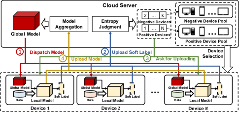
Figure 1 details both the architecture of and the workflow for FedEntropy, where one training round of FedEntropy involves four steps. Unlike transitional FL, on the cloud FedEntropy maintains two pools of device indices, i.e., positive device pool and negative device pool, where initially the positive device pool contains all the devices. At the beginning of a training round, the cloud server randomly selects partial (i.e., with the number of where ) devices from either positive pool or negative pool according to the -greedy policy. In step 1 the cloud broadcasts the global model to all the selected devices. Once the selected devices finish the local training, in step 2 they only forward their soft labels to the server. Note that, compared with the size of a local model, the size of a soft label is negligible. All the collected soft labels will then be processed by the maximum entropy judgment module of the cloud, where labels that lead to maximum aggregated information entropy will be used for fine-grained device grouping. For all the selected devices in this training round, we mark the devices whose soft labels contribute to the maximum entropy as positive devices, while the other remaining devices are marked as negative devices. In step 3, only the positive devices need to upload their local models for the aggregation, which will be executed in step 4. At the end of each round, the positive devices and negative devices will be put into the positive device pool and negative device pool, respectively.
3.3 Maximum Entropy Judgment
Our approach adopts entropy to judge the similarity between the data distributions of devices. To accurately calculate such information entropy, it is required to obtain the probability distributions of datasets from devices. However, if all the devices send their datasets to the cloud, the FL assumption of data privacy will be substantially violated DBLP:conf/infocom/WangSZSWQ19 . Instead of sending datasets directly to the cloud, our approach adopts the averaged soft label information of samples to implicitly represent the dataset distributions of devices. In this way, the data privacy of devices can be guaranteed.
Based on the outputs of the softmax layer of a local model, we collect all the soft labels of samples including the ones of both correct and incorrect predictions, where a soft label indicates the data distribution within a sample. We then aggregate these soft labels together to form an indicator of the data distribution of all samples on the same device. For a device with an index of , assuming that it has samples, we calculate the data distribution of corresponding device by averaging all its soft labels using the formula as follows:
where denotes the softmax layer output of the local model when the input is . Assume that in one FL training round, a set of devices are selected whose sample distributions form a set . Assuming that there are data categories in total for the whole FL training, the information entropy for the probability distribution is defined as follows:
According to the intrinsic property of information entropy, only when the data distribution of selected devices is uniform, we can achieve the highest information entropy. Based on the observation in DBLP:journals/tpds/DuanLCLTL21 , when the overall data distributions on the selected devices is uniform (i.e., the datasets are complementary to each other), we can achieve the best aggregation quality. In other words, the higher the overall entropy of soft labels sent by selected devices is , the better the aggregation quality we can achieve. However, it is hard to achieve such a uniform distribution in FL, especially for non-IID scenarios. In order to make an entropy of some device group as high as possible, we design a maximum entropy judgement, which can effectively filter the devices that has negative impacts on the maximum entropy calculation.
Algorithm 1 details the implementation of our maximum entropy judgment module on the cloud. Note that the inputs of this algorithms include the aggregated soft labels of selected devices and their corresponding dataset sizes. In this algorithm, initially we use to save all the collected aggregated soft labels. Then, our approach iteratively searches for soft labels in that can degrade the overall entropy of data distributions of selected devices, until no aggregated soft label in the positive device set (i.e., ) is harmful to the overall entropy. Line 1 initializes and , where denotes the set of devices that are filtered away from . Lines 2-19 iteratively judge whether there exist aggregated soft labels that are harmful for the overall entropy. Line 3 recalculates the overall entropy of the aggregated soft labels for positive devices based on the formula as follows:
Lines 4-12 traverse all the aggregated soft labels to detect whether there exists one that is harmful for the overall entropy. If exist, lines 16-17 will remove the corresponding device from the positive device set and put it to the negative device set. Otherwise, line 14 will terminate the search. Finally, line 20 returns the judgment results based on the concept of maximum entropy.
3.4 Implementation of FedEntropy
As shown in Figure 1, our approach maintains two pools for positive devices and negative devices, respectively. Although the devices in the positive device pool can contribute more to the overall entropy, it does not mean the datasets of negative devices are useless. In fact, the main reason that a device is in the negative device pool is because it fails to get on well with majority of devices involved in FL. In order to encourage all the devices to participate the global model aggregation, we propose a dynamic device grouping strategy. At the beginning of each training round, the cloud uses the -greedy policy to select devices from either the positive pool (with a probability of ) or the negative pool (with a probability of ), where by default. If the number of devices in one pool is insufficient, our approach will randomly select the remaining devices from the other pool. Based on this cloud setting, our FedEntropy method is implemented as follows.
Algorithm 2 details the interactions between the cloud server and devices during the training of FedEntropy, where lines 3-23 conduct rounds of FedEntropy training. Based on the -greedy policy, lines 4-8 select a set devices from either the positive pool or the negative pool. Line 9 initializes , , and , which are used for storing corresponding soft labels, models, and dataset sizes of selected devices, respectively. In lines 10-13, the cloud broadcasts the global model to all the selected devices in to trigger local training by the devices in parallel. After collecting all the aggregated labels from selected devices, line 14 figures out both the positive devices and negative devices for the aggregation using the function JudgeEntropy implemented in Algorithm 1. In lines 15-20, the cloud asks the positive devices in to upload their local models for the aggregation in line 21. Meanwhile, both positive and negative device pools are updated in line 22. Finally, the algorithm achieves a trained global model for all the involved devices in some non-IID scenario.
Convergence Analysis and Discussions. Similar to DBLP:journals/corr/abs-2203-09249 , we use FedAvg as the FL optimizer of FedEntropy. As stated in li2019convergence , FedAvg converges at a rate of . Since FedEntropy selectively aggregates a portion of devices per round, we can reasonably regard FedEntropy as a variant of FedAvg that aggregates a subset of selected devices per round. Therefore, both FedEntropy and FedAvg have the same convergence rate, i.e., . Note that, FedEntropy can also adopt other existing FL methods as its optimizer, where the convergence rate of FedEntropy is the same as theirs.
4 Experiments
To evaluate the effectiveness of our approach, we implemented our FedEntropy framework using PyTorch. All the experimental results were obtained on a Ubuntu workstation with Intel i9-10900k CPU, 32GB RAM, and NVIDIA GeForce RTX 3080 GPU.
4.1 Experimental Settings
Baseline Methods. We compared FedEntropy with four FL methods including the classic one and three state-of-the-arts, i.e., FedAvg mcmahan2017communication , FedProx li2020federated , SCAFFOLD karimireddy2019scaffold and Moon li2021model . Note that, by default, we used FedAvg as the FL optimizer in FedEntropy.
Dataset and DNN Settings. To facilitate the performance comparison, we evaluated the FL methods on three well-known benchmark datasets, i.e., CIFAR-10, CIFAR-100 krizhevsky2009learning and CINIC-10 DBLP:journals/corr/abs-1810-03505 , where the images of CINIC-10 come from ImageNet DBLP:journals/corr/ChrabaszczLH17 and CIFAR-10. Note that the CIFAR-100 dataset has two kinds of sample labels, i.e., fine-grained labels (with 100 classes) and coarse-grained labels (with 20 superclasses). To better evaluate the performance of different FL methods, we adopted the coarse-grained labels for classification. Similar to dataset distribution settings in wang2020optimizing ; DBLP:conf/iclr/AcarZNMWS21 ; DBLP:conf/icml/YurochkinAGGHK19 , we adopted three kinds of data distributions to reflect the data heterogeneity: i) case 1 where data on each device belong to the same single label; ii) case 2 where data on each device belong to two labels evenly; and iii) case 3 where data follow the Dirichlet distribution ( by default). Note that we can tune the value of to control the heterogeneity of non-IID data among devices, where a smaller indicates higher data heterogeneity. For all the three datasets, we used the DNN models with the same architecture. To be specific, each DNN model here has two 55 convolution layers. The first layer has 6 output channels and the second layer has 16 output channels, where each layer is followed by a 22 max pooling operation. Please refer to Appendix A.1 for more details about the settings for datasets and DNNs.
| Dataset | Heterogeneity Settings | Test Accuracy() | ||||
| FedAvg | FedProx | SCAFFOLD | Moon | Ours | ||
| CIFAR-10 | case 1 | 27.080.79 | 27.590.55 | 22.301.85 | 22.101.30 | 32.521.05 |
| case 2 | 48.900.47 | 49.220.25 | 48.731.62 | 46.860.39 | 51.391.18 | |
| case 3 | 48.310.83 | 47.770.78 | 50.491.21 | 47.380.53 | 51.000.23 | |
| CIFAR-100 | case 1 | 15.390.86 | 15.130.96 | 14.490.73 | 11.860.49 | 18.470.75 |
| case 2 | 27.620.44 | 27.250.14 | 28.420.22 | 27.110.0.58 | 29.240.70 | |
| case 3 | 28.710.22 | 28.470.49 | 30.150.50 | 28.130.21 | 29.210.25 | |
| CINIC-10 | case 1 | 23.231.87 | 23.541.07 | 20.270.90 | 20.341.76 | 29.341.48 |
| case 2 | 36.090.85 | 36.630.97 | 35.861.68 | 36.120.92 | 37.650.45 | |
| case 3 | 34.111.39 | 34.350.94 | 37.520.43 | 33.900.57 | 35.840.70 | |
| FL Method | Communication Rounds | ||
| case 1(acc = 30%) | case 2 (acc = 50%) | case 3 (acc = 50%) | |
| FedAvg | 591.3325.32 | 316.0037.59 | 359.67239.12 |
| FedProx | 569.33122.50 | 248.0022.61 | 279.3348.09 |
| SCAFFOLD | 793.00159.42 | 339.6724.95 | 291.3315.89 |
| Moon | 853.67+67.83 | 297.3335.16 | 310.0045.90 |
| Ours | 340.0052.20 | 193.3313.50 | 223.6769.06 |
Hyperparameters. For FedEntropy, we set the threshold to 0.8. For FedProx, we set the hyperparameter to 0.01, which controls the proximal term weight. For SCAFFOLD, we set the global step-size to 1. Similar to the settings in li2021model , for Moon we set the hyperparameters to 0.1 and temperature to 0.5. For all FL methods, we set the number of clients (i.e., ) to 100, and the number of communication rounds (i.e., ) to 1000. To mimic real-world scenarios with limited communication resources, we set the ratio of participant devices in each FL training round to 10% (i.e., = 10). For each device, the local optimizer is with a learning rate of 0.01 and a momentum of 0.5. For local training, we set the batch size to 50 and the number of local training epochs (i.e., ) to 5.
4.2 Performance Comparison
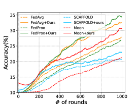
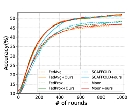
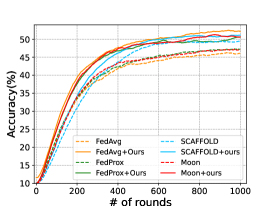
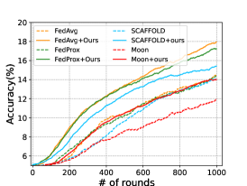
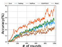
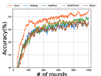
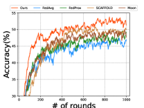
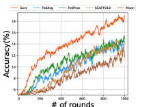
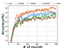
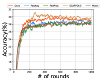
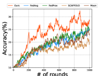
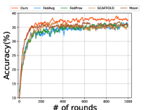
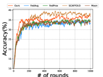
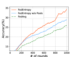
Test Accuracy. Table 1 presents the performance comparison results between our FedEntropy and the four baseline methods in terms of test accuracy. To enable a fair comparison, all the experiments were repeated 3 times with different random seeds, and we calculated the average results of the last ten rounds. From Table 1, we can find that under different data heterogeneity settings, FedEntropy outperforms other FL methods with a considerable improvement. Taking the case 1 of CIFAR-10 as an example, the test accuracy of our FedEntropy is 5.44%, 4.93%, 10.22%, and 10.42% higher than FedAvg, FedProx, SCAFFOLD, and Moon, respectively. Figure 2 presents the accuracy trends of all the five studied FL methods on the three datasets with different data heterogeneity settings. From Figure 2, we can find that in most cases FedEntropy can not only achieve the highest accuracy, but also converge faster than the other FL methods for a given accuracy.
| Combination | Test Accuracy() | ||
| case 1 | case 2 | case 3 | |
| FedAvg + FedEntropy | 40.740.88 | 54.210.12 | 53.961.55 |
| FedProx + FedEntropy | 40.441.81 | 53.780.87 | 53.370.56 |
| SCAFFOLD + FedEntropy | 30.201.14 | 52.280.89 | 53.470.21 |
| Moon + FedEntropy | 35.972.78 | 53.910.87 | 52.920.83 |
Communication Overhead. Considering that the downlink communication overhead of all FL methods is consistent, here we only consider the communication overhead of uploading local models. For FedAvg, FedProx and Moon, the communication overhead per round is only for uploading the models of selected devices. However, for SCAFFOLD, in each round it additionally requires uploading the local control variables of selected devices, whose sizes are the same as the ones of local models. In other words, the communication cost of SCAFFOLD is twice that of traditional FL methods. In the first stage of device selection, FedEntropy firstly uploads the soft labels of selected devices to the cloud. Since the data volume of soft labels is much smaller than one of the local models, such communication overhead is negligible. For the second stage, under maximum entropy judgment, the communication overhead of FedEntropy per round is at most the same as the one of FedAvg. Table 2 presents the communication overhead required by the five FL methods to achieve the same accuracy for different non-IID scenarios of CIFAR-10. For the three different non-IID scenarios, we set the expected accuracy to 30%, 50%, and 50%, respectively. We can find that FedEntropy has the least number of communication rounds and the least communication overhead in all scenarios. Note that we can observe the similar trends for the other two datasets.
Synergy between FedEntropy and other FL methods. Table 3 presents the performance of FedEntropy using FedAvg, FedProx, SCAFFOLD, and Moon as optimizers. Compared with the results in Table 1, we can find that the classification performance of all the four FL methods under the help of our maximum entropy-based dynamic device grouping is improved significantly. In other words, our dynamic device grouping can be integrated into other FL methods to enhance their classification performance, showing the orthogonality of FedEntropy for other FL methods. By simply applying our dynamic device grouping method on FedAvg, the results in Table 1 and Table 3 show that the classification performance of FedAvg+FedEntropy can even outperform SCAFFOLD.
4.3 Ablation Study
We conducted ablation studies to demonstrate the impact of our proposed dynamic device grouping method used in FedEntropy and the impact of components (maximum entropy judgment and positive/negative device pools) in FedEntropy. Figure 3a shows the results on the case 1 of CIFAR-10. We can find that under the help of FedEntropy, both the accuracy and convergence of four FL baseline methods are dramatically improved. Please refer to Appendix A.3 for more results on other cases and datasets. Figure 3b investigates the impacts of key FedEntropy components. Here, we consider three cases: i) FedEntropy, ii) FedEntropy without positive/negative device pools, and iii) FedAvg. Note that for the second case, we assume that all the selected devices are all put in the positive device pool. We can find that both two components on cloud introduced by our proposed FedEntropy can indeed greatly increase the classification accuracy. Due to the space limitation, Figure 3b only presents the comparison results for the case 1 of CIFAR-10, the other cases with the same or different datasets have the same trends as the one shown here.
5 Conclusion
To accommodate the biased device data distributions in non-IID scenarios, in this paper we proposed a novel FL framework named FedEntropy, which takes both the data distributions of devices and contributions of local models to global model aggregation into account. Based on our maximum entropy judgement heuristic, we designed a two-stage device grouping method to enable fine-grained selection of more suitable local models to achieve better aggregation quality. Comprehensive experimental results on various well-known benchmarks show that, compared with state-of-the-art FL methods, FedEntropy not only can achieve better FL performance in terms of both classification accuracy and communication overhead, but also can be used to enhance their classification performance.
References
- [1] Brendan McMahan, Eider Moore, Daniel Ramage, Seth Hampson, and Blaise Agüera y Arcas. Communication-efficient learning of deep networks from decentralized data. In AISTATS, pages 1273–1282, 2017.
- [2] Avishek Ghosh, Jichan Chung, Dong Yin, and Kannan Ramchandran. An efficient framework for clustered federated learning. In NeurIPS, pages 19586–19597, 2020.
- [3] Aritra Mitra, Rayana H. Jaafar, George J. Pappas, and Hamed Hassani. Linear convergence in federated learning: Tackling client heterogeneity and sparse gradients. In NeurIPS, pages 14606–14619, 2021.
- [4] Naman Agarwal, Peter Kairouz, and Ziyu Liu. The skellam mechanism for differentially private federated learning. In NeurIPS, pages 5052–5064, 2021.
- [5] Mi Luo, Fei Chen, Dapeng Hu, Yifan Zhang, Jian Liang, and Jiashi Feng. No fear of heterogeneity: Classifier calibration for federated learning with non-iid data. In NeurIPS, pages 5972–5984, 2021.
- [6] Sai Praneeth Karimireddy, Martin Jaggi, Satyen Kale, Mehryar Mohri, Sashank J. Reddi, Sebastian U. Stich, and Ananda Theertha Suresh. Breaking the centralized barrier for cross-device federated learning. In NeurIPS, pages 28663–28676, 2021.
- [7] Ahmed Khaled, Konstantin Mishchenko, and Peter Richtárik. Tighter theory for local SGD on identical and heterogeneous data. In AISTATS, pages 4519–4529, 2020.
- [8] Tian Li, Anit Kumar Sahu, Manzil Zaheer, Maziar Sanjabi, Ameet Talwalkar, and Virginia Smith. Federated optimization in heterogeneous networks. In MLSys, pages 429–450, 2020.
- [9] Sai Praneeth Karimireddy, Satyen Kale, Mehryar Mohri, Sashank J. Reddi, Sebastian U. Stich, and Ananda Theertha Suresh. SCAFFOLD: stochastic controlled averaging for federated learning. In ICML, pages 5132–5143, 2020.
- [10] Qinbin Li, Bingsheng He, and Dawn Song. Model-contrastive federated learning. In CVPR, pages 10713–10722, 2021.
- [11] Cheng Chen, Ziyi Chen, Yi Zhou, and Bhavya Kailkhura. Fedcluster: Boosting the convergence of federated learning via cluster-cycling. In BigData, pages 5017–5026, 2020.
- [12] Yann Fraboni, Richard Vidal, Laetitia Kameni, and Marco Lorenzi. Clustered sampling: Low-variance and improved representativity for clients selection in federated learning. In ICML, pages 3407–3416, 2021.
- [13] Zhuangdi Zhu, Junyuan Hong, and Jiayu Zhou. Data-free knowledge distillation for heterogeneous federated learning. In ICML, pages 12878–12889, 2021.
- [14] Daliang Li and Junpu Wang. Fedmd: Heterogenous federated learning via model distillation. arXiv preprint arXiv:1910.03581, 2019.
- [15] Tao Lin, Lingjing Kong, Sebastian U. Stich, and Martin Jaggi. Ensemble distillation for robust model fusion in federated learning. In NeurIPS, 2020.
- [16] Hongda Wu and Ping Wang. Node selection toward faster convergence for federated learning on non-iid data. arXiv preprint arXiv:2105.07066, 2021.
- [17] Weiming Zhuang, Yonggang Wen, Xuesen Zhang, Xin Gan, Daiying Yin, Dongzhan Zhou, Shuai Zhang, and Shuai Yi. Performance optimization of federated person re-identification via benchmark analysis. In ACM Multimedia, pages 955–963, 2020.
- [18] Abhimanyu Dubey, Otkrist Gupta, Ramesh Raskar, and Nikhil Naik. Maximum-entropy fine grained classification. In NeurIPS, pages 635–645, 2018.
- [19] Moming Duan, Duo Liu, Xianzhang Chen, Renping Liu, Yujuan Tan, and Liang Liang. Self-balancing federated learning with global imbalanced data in mobile systems. TPDS, 32(1):59–71, 2021.
- [20] Edwin T Jaynes. Information theory and statistical mechanics. Physical review, 106(4):620, 1957.
- [21] Yihua Chen, Eric K. Garcia, Maya R. Gupta, Ali Rahimi, and Luca Cazzanti. Similarity-based classification: Concepts and algorithms. JMLR, 10:747–776, 2009.
- [22] Jun Zhu, Eric P. Xing, and Bo Zhang. Partially observed maximum entropy discrimination markov networks. In NIPS, pages 1977–1984, 2008.
- [23] John Shawe-Taylor and David R. Hardoon. Pac-bayes analysis of maximum entropy classification. In AISTATS, pages 480–487, 2009.
- [24] Gabriel Pereyra, George Tucker, Jan Chorowski, Lukasz Kaiser, and Geoffrey E. Hinton. Regularizing neural networks by penalizing confident output distributions. In ICLR, 2017.
- [25] Zhibo Wang, Mengkai Song, Zhifei Zhang, Yang Song, Qian Wang, and Hairong Qi. Beyond inferring class representatives: User-level privacy leakage from federated learning. In INFOCOM, pages 2512–2520, 2019.
- [26] Lin Zhang, Li Shen, Liang Ding, Dacheng Tao, and Ling-Yu Duan. Fine-tuning global model via data-free knowledge distillation for non-iid federated learning. arXiv preprint arXiv:2203.09249, 2022.
- [27] Xiang Li, Kaixuan Huang, Wenhao Yang, Shusen Wang, and Zhihua Zhang. On the convergence of fedavg on non-iid data. In ICLR, 2020.
- [28] Alex Krizhevsky, Geoffrey Hinton, et al. Learning multiple layers of features from tiny images. In Citeseer, 2009.
- [29] Luke Nicholas Darlow, Elliot J. Crowley, Antreas Antoniou, and Amos J. Storkey. CINIC-10 is not imagenet or CIFAR-10. arXiv preprint arXiv:1810.03505, 2018.
- [30] Patryk Chrabaszcz, Ilya Loshchilov, and Frank Hutter. A downsampled variant of imagenet as an alternative to the CIFAR datasets. arXiv preprint arXiv:1707.08819, 2017.
- [31] Hao Wang, Zakhary Kaplan, Di Niu, and Baochun Li. Optimizing federated learning on non-iid data with reinforcement learning. In INFOCOM, pages 1698–1707, 2020.
- [32] Durmus Alp Emre Acar, Yue Zhao, Ramon Matas Navarro, Matthew Mattina, Paul N. Whatmough, and Venkatesh Saligrama. Federated learning based on dynamic regularization. In ICLR, 2021.
- [33] Mikhail Yurochkin, Mayank Agarwal, Soumya Ghosh, Kristjan H. Greenewald, Trong Nghia Hoang, and Yasaman Khazaeni. Bayesian nonparametric federated learning of neural networks. In ICML, pages 7252–7261, 2019.
Appendix A Appendix
A.1 Dataset and Model Settings
Table 4 details the dataset settings used in the experiments. Table 5 presents the settings for CNNs used in the experiments.
| Dataset | Input Size | Classes | Training Images | Test Images |
| CIFAR-10 | 33232 | 10 | 50000 | 10000 |
| CINIC-10 | 33232 | 10 | 90000 | 90000 |
| CIFAR-100 | 33232 | 20 | 50000 | 10000 |
| Layer Index | Type | Parameters |
| 1 | Convolutional | kernel: 55, filter: 6 |
| 2 | Convolutional | kernel: 55, filter: 16 |
| 3 | Fully Connected | unit: 120 |
| 4 | Fully Connected | unit: 84 |
| 5 | Fully Connected | unit: class numbers of dataset |
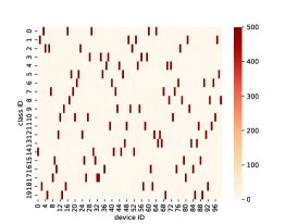
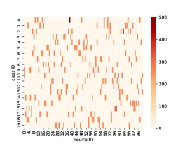
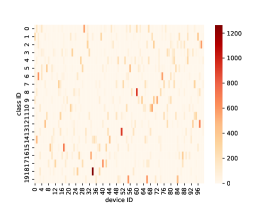
A.2 Visualization of Data Heterogeneity
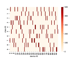
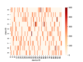
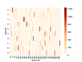
Figure 4 shows the data distributions of clients generated by the three heterogeneous data settings defined in Section 4.1. In each subfigure, we show the data distribution of 100 clients. In Figure 4, the data distribution of clients in different cases is distinctly different, and the degree of data heterogeneity increases from case 1 to case 3.
A.3 Supplementary Experimental Results
In this section, we provide more experiments to show the advantages of FedEntropy, whose code is available at https://github.com/FedEntropy/FedEntropy.
Communication Overhead. For given target test accuracy (i.e., 12%, 28%, 30% correspond for cases 1-3, respectively), Table 6 presents the number of FL communication rounds to reach this reach target. This information is a supplement to Table 2.
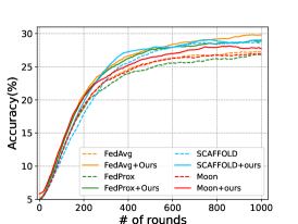
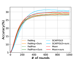
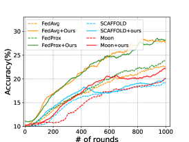
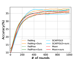
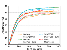
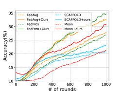
Synergy between FedEntropy and SOTA FL Methods. To evaluate whether our approach can be applied on state-of-the-art methods, Figure 5 presents the accuracy information, where the notation “X+Ours” indicates that a combination of FL method X and our approach. We can find that all the four state-of-the-art FL methods get notable benefits from our approach.
| Communication Rounds | |||
| case 1(acc = 12%) | case 2(acc = 28%) | case 3(acc = 30%) | |
| FedAvg | 206.6711.02 | 233.6715.50 | 155.3317.62 |
| FedProx | 222.6718.50 | 270.6761.58 | 160.006.58 |
| SCAFFOLD | 305.0088.71 | 246.3325.42 | 291.3315.89 |
| Moon | 510.6725.01 | 219.6769.12 | 183.0017.35 |
| Ours | 159.6721.46 | 173.3323.07 | 117.334.04 |