IRS Phase-Shift Feedback Overhead-Aware Model Based on Rank-One Tensor Approximation

Abstract

In this paper, we propose a rank-one tensor modeling approach that yields a compact representation of the optimum intelligent reconfigurable surface (IRS) phase-shift vector for reducing the feedback overhead. The main idea consists of factorizing the IRS phase-shift vector as a Kronecker product of smaller vectors, namely factors. The proposed phase-shift model allows the network to trade-off between achievable data rate and feedback reduction by controling the factorization parameters. Our simulations show that the proposed phase-shift factorization drastically reduces the feedback overhead, while improving the data rate in some scenarios, compared to the state-of-the-art schemes.

I Introduction

IRS is a possible candidate technology for beyond fifth generation (B5G) and sixth generation (6G) networks due to the ability to control the electromagnetic properties of the radio-frequency propagated waves by performing an intelligent phase-shift to the desired direction [1, 2, 3, 4, 5, 6]. Usually, the IRS is defined as a planar ($2$-D) surface with a large number of independent reflective elements in which they can be fully passive or with some elements active [7, 8, 9]. The IRS is connected to a smart controller that sets the desired phase-shift for each reflective element, by applying some bias voltage at the elements e.g., PIN diodes. One main advantage of the fully passive IRSs is its full-duplex nature, i.e., no noise amplification is observed since no signal processing is possible. However, this fully passive nature makes the channel state information acquisition process difficult, since no pilots are processed, thus only the cascade channel can be estimated. Another advantage of an IRS with fully passive elements is that the power consumption is concentrated at the controller. This makes the IRS a more attractive technology in terms of energy efficient compared to others, e.g., amplify-and-forward and decode-and-forward relays [10].

The work of [11] proposes a protocol design to maximize the transmission rate in IRS-assisted multiple-input multiple-output (MIMO)-orthogonal frequency division multiplexing (OFDM) systems. Also, [12] proposes a framework for a feedback overhead-aware resource allocation in IRS-assisted MIMO systems.

In this work, we propose a new overhead-aware model for designing the IRS phase-shifts. Our idea is to represent the IRS phase-shift vector according to a rank-one model. This is achieved by factorizing a tensorized version of the IRS phase-shift vector into a rank-one tensor, which is modelled as the Kronecker product of a predefined number of factors. These factors are estimated using a closed-form solution to rank-one tensor approximation. After the estimation process, the phases of the factors are quantized and fed back to the IRS controller, which will reconstruct the IRS phase-shift vector based on its rank-one tensor model. The main contributions of the proposed factorization are the following:

$1)$ The proposed IRS phase-shift factorization allows to save network resources. In other words, the network can perform IRS phase-shift feedback more often, or with a reduced overhead, which significantly improves the end-to-end latency.

$2)$ The proposed method allows a trade-off between the feedback duration and achievable data rate (ADR) performance by properly choosing the parameters of the rank-one model that represents the IRS phase-shift vector. This is an important feature of our proposed method, specially for a limited feedback control link.

$3)$ Our approach relies on the optimum IRS phase-shift vector, which means that, it can be implemented in different IRS-assisted systems and in multiple communication links, i.e., downlink or uplink, in single-input single-output (SISO), multiple-input single-output (MISO), as well in MIMO systems.

I-A Notation and Properties

Scalars are represented as non-bold lower-case letters $a$, column vectors as lower-case boldface letters $\bm{a}$, matrices as upper-case boldface letters $\bm{A}$, and tensors as calligraphic upper-case letters $\bm{\mathcal{A}}$. The superscripts $\{\cdot\}^{\text{T}}$, $\{\cdot\}^{\text{*}}$, $\{\cdot\}^{\text{H}}$ and $\{\cdot\}^{+}$ stand for transpose, conjugate, conjugate transpose and pseudo-inverse operations, respectively. The operator $\Arrowvert\cdot\Arrowvert_{\text{F}}$ denotes the Frobenius norm of a matrix or tensor, $\mathbb{E}\{\cdot\}$ is the expectation operator. The operator $\text{diag}\left(\bm{a}\right)$ converts $\bm{a}$ into a diagonal matrix. Moreover, $\text{vec}\left(\bm{A}\right)$ converts $\bm{A}\in\mathbb{C}^{I_{1}\times R}$ to a column vector $\bm{a}\in\mathbb{C}^{I_{1}R\times 1}$ by stacking its columns on top of each other, while the unvec($\cdot$) operator is the inverse of the vec operation. Also, $\bm{a}_{r}\in\mathbb{C}^{I\times 1}$ represents the $r$-th column of $\bm{A}\in\mathbb{C}^{I\times R}$. The operators $\otimes$ and $\circ$, defines the Kronecker and the outer products, respectively. We make use of the property

$$\bm{a}\otimes\bm{b}=\text{vec}\left(\bm{b}\circ\bm{a}\right).$$ (1)

II Tensor Pre-Requisites

Consider a set of matrices $\{\bm{X}_{i_{3}}\}\in\mathbb{C}^{I_{1}\times I_{2}}$, for $i_{3}=1,\ldots,I_{3}$. By concatenating all $I_{3}$ matrices to form the third-order tensor $\bm{\mathcal{X}}=[\bm{X}_{1}\sqcup_{3}\bm{X}_{2}\sqcup_{3}\ldots\sqcup_{3}\bm{X}_{I_{3}}]\in\mathbb{C}^{I_{1}\times I_{2}\times I_{3}}$, where $\sqcup_{3}$ indicates a concatenation in the third dimension. We can interpret $\bm{X}_{i_{3}}$ as the $i_{3}$-th frontal slice of $\bm{\mathcal{X}}$, defined as $\bm{\mathcal{X}}_{..i_{3}}=\bm{X}_{i_{3}}$ where the “$..$” indicates that the dimensions $I_{1}$ and $I_{2}$ are fixed. The tensor $\bm{\mathcal{X}}$ can be matricized by letting one dimension vary along the rows and the remaining two dimensions along the columns. From $\bm{\mathcal{X}}$, we can form three different matrices, referred to as the $n$-mode unfoldings (for $n=\{1,2,3\}$ in this case),

$$\left[\bm{\mathcal{X}}\right]_{\left(1\right)} =[\bm{\mathcal{X}}_{..1},\ldots,\bm{\mathcal{X}}_{..I_{3}}]\in\mathbb{C}^{I_{1}\times I_{2}I_{3}},$$ (2)

$$\left[\bm{\mathcal{X}}\right]_{\left(2\right)} =[\bm{\mathcal{X}}_{..1}^{\text{T}},\ldots,\bm{\mathcal{X}}_{..I_{3}}^{\text{T}}]\in\mathbb{C}^{I_{2}\times I_{1}I_{3}}$$ (3)

$$\left[\bm{\mathcal{X}}\right]_{\left(3\right)} =[\text{vec}(\bm{\mathcal{X}}_{..1}),\ldots,\text{vec}(\bm{\mathcal{X}}_{..I_{3}})]^{\text{T}}\in\mathbb{C}^{I_{3}\times I_{1}I_{2}}.$$ (4)

II-A Tensorization

The tensorization operation consists of mapping the elements of a vector into high-order tensors. Let us define the vector $\bm{y}\in\mathbb{C}^{N\times 1}$, in which $N=\prod\limits_{p=1}^{P}{N_{p}}$. By applying the tensorization operator, defined as $\bm{\mathcal{T}}\{\cdot\}$, we can form the tensor $\bm{\mathcal{Y}}=\bm{\mathcal{T}}\{\bm{y}\}\in\mathbb{C}^{N_{1}\times N_{2}\times\ldots\times N_{P}}$. The mapping of elements from $\bm{y}$ to $\bm{\mathcal{Y}}$ is defined as

$$\bm{\mathcal{Y}}_{n_{1},n_{2},\ldots,n_{P}}=\bm{y}_{n_{1}+(n_{2}-1)N_{1}+\ldots+(n_{P}-1)N_{P-1}\cdots N_{2}N_{1}},$$ (5)

where $n_{p}=\{1,\ldots,N_{p}\}$, for $p=\{1,\ldots,P\}$. This operator plays a key role on the proposed feedback-aware method where we reshape the elements of the IRS phase-shift vector into a $P$-order tensor.

II-B Rank-One Tensors

A rank-one matrix can be described as the outer product of two vectors. Similarly to the matrix case, a rank-one tensor is given as the outer product of three or more vectors. For a $P$-order rank-one tensor $\bm{\mathcal{Y}}$, it can be written as

$$\bm{\mathcal{Y}}=\bm{a}^{(1)}\circ\bm{a}^{(2)}\circ\ldots\circ\bm{a}^{(P)}\in\mathbb{C}^{I_{1}\times I_{2}\times\ldots\times I_{P}},$$ (6)

where $\bm{a}^{(p)}\in\mathbb{C}^{I_{p}\times 1}$ is the $p$-th factor of $\bm{\mathcal{Y}}$, for $p=\{1,\ldots,P\}$. The $p$-th rank-one matrix unfolding of $\bm{\mathcal{Y}}$, defined as $\left[\bm{\mathcal{Y}}\right]_{\left(P\right)}\in\mathbb{C}^{I_{p}\times I_{1}\cdots I_{p-1}I_{p+1}\cdots I_{P}}$, is given by

$$\left[\bm{\mathcal{Y}}\right]_{\left(p\right)}=\bm{a}^{(p)}\left(\bm{a}^{(P)}\otimes\ldots\otimes\bm{a}^{(p+1)}\otimes\bm{a}^{(p-1)}\ldots\otimes\bm{a}^{(1)}\right)^{\text{T}}.$$ (7)

Defining $\bm{y}=\text{vec}\left(\bm{\mathcal{Y}}\right)\in\mathbb{C}^{I_{1}\cdots I_{P}\times 1}$ and using (1), we have

$$\bm{y}=\bm{a}^{(P)}\otimes\ldots\otimes\bm{a}^{(1)}.$$ (8)

III System Model

We consider an IRS-assisted MIMO system, where the transmitter (TX) is equipped with a uniform linear array (ULA) with $M_{T}$ antenna elements, the receiver (RX) is equipped with ULA with $M_{R}$ antenna elements and the IRS has $N$ reflective elements. To simplify the discussions, let us consider a single stream transmission, assuming that there is no direct link between the TX and RX. First, the TX sends a pilot signal to the RX with the aid of the IRS. Since there is no signal processing at the IRS, the channel estimation and the IRS phase-shifts optimization are performed at the RX. The received signal after processing the pilots is given by

$$y=\bm{w}^{\text{H}}\bm{G}\bm{S}\bm{H}\bm{q}+\bm{w}^{\text{H}}\bm{b},$$ (9)

where $\bm{b}\in\mathbb{C}^{M_{R}\times 1}$ is the additive noise at the receiver with $\mathbb{E}[\bm{b}\bm{b}^{\text{H}}]=\sigma^{2}_{b}\bm{I}_{M_{r}}$, $\bm{w}\in\mathbb{C}^{M_{R}\times 1}$ and $\bm{q}\in\mathbb{C}^{M_{T}\times 1}$ are the receiver and transmitter combiner and precoder, respectively. $\bm{H}\in\mathbb{C}^{N\times M_{T}}$ and $\bm{G}\in\mathbb{C}^{M_{R}\times N}$ are the TX-IRS and IRS-RX involved channels, and $\bm{S}=\text{diag}(\bm{s})\in\mathbb{C}^{N\times N}$ where $\bm{s}=[e^{j\theta_{1}},\ldots,e^{j\theta_{N}}]\in\mathbb{C}^{N\times 1}$ is the IRS phase-shift vector, and $\theta_{n}$ is the phase-shift applied to the $n$-th IRS element.

After the channel estimation step, an optimization step of the precoder and combiner (active beamformers) vectors $\bm{w}$ and $\bm{q}$, and the IRS phase-shift vector $\bm{s}$ (passive beamformer) is performed. Later, the RX needs to feedback to the IRS controller the designed phase-shift so that the elements can reconfigure the elements to have the optimal phase-shift. From the fact that this feedback may occur through a limited control channel and that the IRS may contain several hundreds to thousand of elements, the feedback of each phase-shift with a certain resolution implies in a signaling overhead.

Related to the issue of the overhead IRS phase-shift signaling feedback, the work of [12] models the feedback duration as

$$T_{\text{F}}=\frac{Nb_{\text{F}}}{B_{\text{F}}\text{log}\left(1+\frac{p_{\text{F}}|{g}_{\text{F}}|^{2}}{B_{\text{F}}N_{0}}\right)},$$ (10)

where $N$ is the total number of phase-shifts of the IRS to be fed back, $B_{\text{F}}$, $p_{\text{F}}$ are the feedback bandwith and power, $g_{\text{F}}$ is the scalar control channel used, $b_{\text{F}}$ is the resolution of each phase-shift, and $N_{0}$ is the noise power density.

IV Proposed Feedback-Aware Method

In this section, we describe our proposed feedback-aware method that focuses on reducing the feedback duration $T_{\text{F}}$, given in (10). Suppose that the channels $\bm{H}$ and $\bm{G}$ are estimated at the RX. Then, the $N$ phase-shifts of the IRS are determined based on state-of-the-art algorithm [12], and are represented in a vector format as $\bm{s}=[e^{j\theta_{1}},e^{j\theta_{2}},\ldots,e^{j\theta_{N}}]\in\mathbb{C}^{N\times 1}$. Our idea is to factorize $\bm{s}$ as the Kronecker product of $P$ factors, i.e.,

$$\bm{s}=\bm{s}^{(P)}\otimes\ldots\otimes\bm{s}^{(1)}\in\mathbb{C}^{N_{P}\cdots N_{1}\times 1}$$ (11)

where $\bm{s}^{(p)}\in\mathbb{C}^{N_{p}\times 1}$ $p$-th factor. From (11), we have that $N=\prod\limits_{p=1}^{P}N_{p}$. The main idea of the proposed model is to feedback to the IRS controller only the phase-shifts of the factors, $\bm{s}^{(p)}$, for $p=\{1,\ldots,P\}$, which results into the feedback of $\sum\limits_{p=1}^{P}N_{p}$ phase-shifts, instead of $N=\prod\limits_{p=1}^{P}$ phase-shifts in the case with no factorization.

Example: To illustrate the impact of this factorization on the IRS phase-shift feedback duration, let us consider the simple scenario, illustrated in Figure 1, where we have an IRS with $N=1024$ elements. Normally, supposing $N$ independent elements, in Figure 1 (a), $N=1024$ phase-shifts would have to be determined at some system node and conveyed to the IRS controller. On the other hand, considering that, as one example, $P=3$ with the following factors $\bm{s}^{(1)}=[e^{j\theta^{(1)}_{1}},\ldots,e^{j\theta^{(1)}_{64}}]\in\mathbb{C}^{64\times 1}$, $\bm{s}^{(2)}=[e^{j\theta^{(2)}_{1}},\ldots,e^{j\theta^{(2)}_{8}}]\in\mathbb{C}^{8\times 1}$ and $\bm{s}^{(3)}=[e^{j\theta^{(3)}_{1}},e^{j\theta^{(3)}_{2}}]\in\mathbb{C}^{2\times 1}$, i.e., $N_{1}=64$, $N_{2}=8$ and $N_{3}=2$, only $N_{1}+N_{2}+N_{3}=74$ phase-shifts has to be reported to the IRS controller, drastically reducing the feedback overhead compared to the traditional scenario (a), by a factor of $\approx 1400\%$. $\blacksquare$

With the factorization, an additional complexity is introduced on the IRS controller, which will have to build the phase-shift vector, which in this case is given as $\bm{s}=\bm{s}^{(3)}\otimes\bm{s}^{(2)}\otimes\bm{s}^{(1)}\in\mathbb{C}^{1024\times 1}$. Physically, the Kronecker product in (11) represents a summation of the factors phase-shifts, as shown in Figure 1 (b). The proposed feedback duration is given by

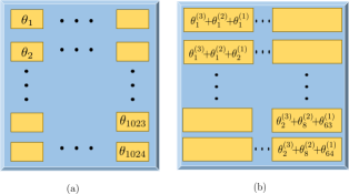
Figure 1: (a) IRS with $N$ phase-shifts, without the factorization, (b) IRS with $N$ phase-shifts factorized into $P=3$ factors.

$$T_{\text{F}}^{\text{prop}}=\frac{T_{\text{PR}}+\sum\limits_{p=1}^{P}N_{p}b^{(p)}_{\text{F}}}{B_{\text{F}}\text{log}\left(1+\frac{p_{\text{F}}|{g}_{\text{F}}|^{2}}{B_{\text{F}}N_{0}}\right)},$$ (12)

where $T_{PR}$ is the duration of the preamble that informs the values of the factorization parameters, such as the number of factors $P$, the size of each factor $N_{p}$, and the number of quantization bits used for each factor $b^{(p)}_{\text{F}}$, for $p=\{1,\ldots,P\}$.

The physical implications on the choice of the proposed rank-one tensor approximation parameters, i.e., the number of the factors $P$ and the size of each factor $N_{p}$ are discussed in Section IV-C. In a general view, the proposed factorization consists of three steps:

$1)$ Rearrangement of elements: In this step, the optimum phase-shift vector $\bm{s}\in\mathbb{C}^{N\times 1}$ is rearranged into a $P$-th order tensor $\bm{\mathcal{S}}\in\mathbb{C}^{N_{1}\times N_{2}\times\ldots\times N_{P}}$, with $N=\prod\limits_{p=1}^{P}N_{p}$. This is accomplished by mapping the elements of the IRS phase-shift vector $\bm{s}$ into the tensor $\bm{S}$, using the tensorization operator, given in (5).

$2)$ Rank-One tensor approxmation: In this step, the RX estimates the factors of the IRS phase-shift tensor $\bm{\mathcal{S}}$. For this, a prior art rank-one tensor estimation algorithmz can be employed, such as the high order singular value decomposition (HOSVD) [13], which is described in Algorithm 1.

$3)$ Normalization: The estimated factors have their entries normalized to ensure the unitary modulus constraint of the IRS phase-shift vector. This can be achieved by only taking the angles of the estimated factors.

IV-A Rank-One IRS model

After the tensorization step, the RX will approximate the optimum phase-shift tensor $\bm{\mathcal{S}}$ using a rank-one model, i.e.,

$$\bm{\mathcal{S}}\approx\bm{s}^{(1)}\circ\ldots\circ\bm{s}^{(P)}\in\mathbb{C}^{N_{1}\times\cdots\times N_{P}}.$$ (13)

Please note that, the approximation comes from the fact that we are fitting independent phase-shifts as a combination of $P$ sets of phase-shifts, thus an approximation error is expected. However, as it will be explained in Section  V, for scenarios with moderate/strong line of sight (LOS) components (approximated rank-one channels), which is the case of interest in IRS networks, this fitting error is negligible on the ADR performance.

The RX estimates the factor components solving the following problem

$$\left[\bm{\hat{s}}^{(1)},\ldots,\bm{\hat{s}}^{(P)}\right]=\underset{\bm{s}^{(1)},\ldots,\bm{s}^{(P)}}{\text{argmin}}\left|\left|\bm{\mathcal{S}}-\bm{s}^{(1)}\circ\ldots\circ\bm{s}^{(P)}\right|\right|^{2}_{\text{F}},$$ (14)

where $\bm{s}^{(p)}\in\mathbb{C}^{N_{p}\times 1}$ is the $p$-th factor. From (7), the $p$-mode unfolding of $\bm{\mathcal{S}}$, defined as $\left[\bm{\mathcal{S}}\right]_{\left(p\right)}\in\mathbb{C}^{N_{p}\times N_{1}\cdots N_{p-1}N_{p+1}\cdots N_{P}}$, is the approximated rank-one matrix, given as

$$\left[\bm{\mathcal{S}}\right]_{\left(p\right)}\approx\bm{s}^{(p)}\left(\bm{s}^{(P)}\otimes\ldots\otimes\bm{s}^{(p+1)}\otimes\bm{s}^{(p-1)}\otimes\ldots\otimes\bm{s}^{(1)}\right)^{\text{T}}.$$ (15)

1:Inputs: Tensor $\bm{\mathcal{S}}$

2:for $p=1:P$ do

3:     Define the SVD of $\left[\bm{\mathcal{S}}\right]_{\left(p\right)}$ as $\bm{U}^{(p)}\bm{\Sigma}^{(p)}\bm{V}^{(p)\text{H}}$, compute an estimate of the $p$-th factor $\bm{s}^{(p)}$ as

$$\bm{\hat{s}}^{(p)}=e^{j\angle\bm{u}_{.1}^{(p)}}$$

4:end for

5:Return $\bm{\hat{s}}^{(1)}$, $\ldots$, $\bm{\hat{s}}^{(P)}$.

Algorithm 1 Feedback-Aware Rank-One Approximation

To solve the problem in (14), we make use of the rank-one HOSVD, which consists of computing, a singular value decomposition (SVD) for each unfolding of $\bm{\mathcal{S}}$ to extract the left dominant singular vector, i.e., considering the SVD of the $p$-th unfolding of $\bm{\mathcal{S}}$, $\left[\bm{\mathcal{S}}\right]_{\left(p\right)}$ as $\bm{U}^{(p)}\bm{\Sigma}^{(p)}\bm{V}^{(p)\text{H}}$, the algorithm set an estimation for the $p$-th factor $\bm{s}^{(p)}$ as $\bm{\hat{s}}^{(p)}=e^{j\angle\bm{u}_{.1}^{(p)}}\in\mathbb{C}^{N_{p}\times 1}$, where $\bm{u}_{.1}^{(p)}$ is the dominant left singular vector of $\bm{s}^{(p)}$.

IV-B Phase-shift Quantization and Feedback

It is important to mention that, after the rank-one factor estimation procedure in Algorithm 1, the RX quantizes the phase-shifts of each factor with $b_{F}^{(p)}$ bits. Let us define $\bm{\tilde{s}}^{(p)}\in\mathbb{C}^{N_{p}\times 1}$ as the $p$-factor after the quantization process, i.e., $\bm{\tilde{s}}^{(p)}=\mathcal{Q}\left\{\bm{\hat{s}}^{(p)},b_{\text{F}}^{(p)}\right\}$. Then, the phase-shifts of the $P$ factors are conveyed to the IRS controller via a control link channel. Finally, the IRS controller reconstructs the IRS phase-shift vector as

$$\bm{s}=\bm{\tilde{s}}^{(P)}\otimes\ldots\otimes\bm{\tilde{s}}^{(1)}\in\mathbb{C}^{N\times 1}.$$ (16)

As observed, the proposed method allows the system to adapt the phase-shift resolution of the factors depending on the control link availability. This feature is very important in order to minimize the performance loss, in the case of limited control link.

IV-C On the Effect of the Factorization Parameters

In this section, we discuss the choice of the factorization parameters and the system performance implications.

Number of factors $P$: This parameter defines the total number of factors used in the rank-one tensor approximation. Its minimum value for the proposed factorization is $P=2$, i.e., the value $P=1$ means that no factorization is employed. By increasing the value of $P$, the number of factors of the factorization model is increased, allowing to reduce the size of the factor components $N_{p}$, consequentially, increasing $P$ reduces the phase-shift feedback overhead.

Size of factor components $N_{p}$: The size of the factor components indicates the total number of independent phase-shifts in the proposed solution, which it also affects the performance. For example, for $N=256$ and choosing $P=2$, two possible configurations are $N_{1}=128$, $N_{2}=2$ and $N_{1}=N_{2}=16$. For the first choice, the system has more independent phase-shifts ($130$), thus a higher spectral efficiency. However, its feedback overhead is higher than that of second configuration that requires only $32$ phase-shifts to be reported in the feedback channel.

V Simulation Results

In this section, we evaluate the performance of the proposed IRS phase-shift overhead-aware feedback model in terms of feedback duration and ADR. For a fair comparison between the proposed rank-one model and the state-of-the-art, we optimize the precoder ($\bm{q}$), combiner ($\bm{w}$), and the IRS phase-shifts ($\bm{s}$) using the upper-bound algorithm of the state-of-the-art [12]. In this case, they are given as

$$\bm{w}=\bm{U}^{(\text{G})}_{.1},\hskip 2.84544pt\bm{q}=\bm{V}^{(\text{H})}_{.1},\hskip 2.84544pt\bm{s}_{n}=e^{-\angle\left(\bm{V}^{\text{G})}_{n,1}\cdot\bm{U}^{(\text{H})}_{n,1}\right)},n=\{1,\ldots,N\},$$

where $\bm{U}^{(\text{G})}_{.1}\in\mathbb{C}^{M_{R}\times 1}$, $\bm{V}^{\text{G})}_{.1}\in\mathbb{C}^{N\times 1}$ are the dominant left and right singular vectors of $\bm{G}$, while $\bm{U}^{(\text{H})}_{.1}\in\mathbb{C}^{N\times 1}$, $\bm{V}^{\text{H})}_{.1}\in\mathbb{C}^{M_{T}\times 1}$ are the dominant left and right singular vectors of $\bm{H}$. The ADR is given by

$$\text{ADR}=\text{log}_{2}\left(1+\frac{\left|\bm{w}^{\text{H}}\bm{G}\bm{S}\bm{H}\bm{q}\right|^{2}}{\sigma^{2}_{b}}\right),$$ (17)

where, the noise variance $\sigma^{2}_{b}=0.1$, $\bm{S}=\text{diag}(\bm{s})\in\mathbb{C}^{N\times 1}$ is the matrix that contains in its diagonal the optimized feedback phase-shifts, which, in the proposed approach is given in (16). Regarding the involved channels, in (9), they are modelled as

$$\bm{H} =\sqrt{\alpha_{H}\frac{K_{H}}{K_{H}+1}}\bm{H}_{\text{LOS}}+\sqrt{\frac{1}{K_{H}+1}}\bm{H}_{\text{NLOS}},$$ (18)

$$\bm{G} =\sqrt{\alpha_{G}\frac{K_{G}}{K_{G}+1}}\bm{G}_{\text{LOS}}+\sqrt{\frac{1}{K_{G}+1}}\bm{G}_{\text{NLOS}},$$ (19)

where $\alpha_{H}$ and $\alpha_{G}$ are the path-loss components of the TX-IRS and IRS-RX links, respectively. $K_{H}$ and $K_{G}$ are the Rician factors for the channels $\bm{H}$ and $\bm{G}$, respectively. $\bm{H}_{\text{LOS}}$, $\bm{G}_{\text{LOS}}$ are modelled as geometric-based channels, while the entries of $\bm{H}_{\text{NLOS}}$, $\bm{G}_{\text{NLOS}}$ are modelled as circularly symmetric complex Gaussian random variables, with zero mean an unit variance, i.e., $\bm{H}_{\text{NLOS}}\sim\mathcal{CN}(0,\bm{I}_{M_{T}})$ and $\bm{G}_{\text{NLOS}}\sim\mathcal{CN}(0,\bm{I}_{M_{R}})$. We consider $\alpha_{H}=\alpha_{G}=1$ for experimental purposes, to observe the performance impact of the proposed IRS phase-shift factorization. Also, we consider $K_{H}=K_{G}=K$ as metric for performance evaluation. The details of the channel model are given in Appendix A.

Let us define the vector $\bm{N}_{\text{P}}=\left[N_{1},\ldots,N_{P}\right]^{\text{T}}\in\mathbb{R}^{P\times 1}$ that contains the size of all individual factors, for a certain $P$. Likewise, let us define the vector $\bm{b}^{(\text{P})}_{\text{F}}=\left[b^{(1)}_{\text{F}},\ldots,b^{(P)}_{\text{F}}\right]^{\text{T}}\in\mathbb{R}^{P\times 1}$ that contains the number of bits used for quantization in each factor, for a certain $P$.

Figure 2 illustrates the payload ratio (PR) between the proposed feedback overhead model and state-of-the-art, given by $\text{PR}=N/\left(\sum\limits_{p=1}^{P}N_{p}\right)$. In this figure, we can observe the role of the $P$ in the factorization model. It allows to decrease the size of the factors, consequentially, allows a massive feedback overhead reduction. For example, in this case where $N=1024$, for $P=2$ we observe a maximum feedback overhead reduction when $\bm{N}_{2}=[32,32]$, i.e., we feedback $64$ phase-shifts against the total of $1024$ phase-shifts that the state-of-the-art does, in other words, a feedback duration $16$ times smaller. As $P$ increases, we can improve the feedback overhead reduction, at the point that, for $P=10$, the proposed feedback overhead is more than $50$ times smaller than the state-of-the-art [12].

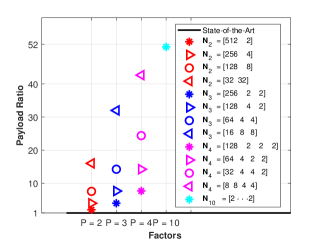
Figure 2: Feedback Payload Ratio for different factors and size configurations. $N=1024$ and $b_{\text{F}}=b^{(p)}_{\text{F}}=3$ bits, for $p=\{1,\ldots,P\}$.

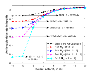
Figure 3: For an IRS with $N=1024$, TX and RX with $M_{R}=M_{T}=2$ and $b^{(p)}_{\text{F}}=b_{\text{F}}=3$ bits, for the IRS phase-shift quantization resolution, for $p=\{1,\ldots,P\}$.

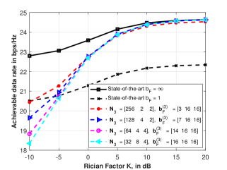
Figure 4: ADR of the state-of-the-art and the proposed factorization for $P=3$ with different size configurations and resolution (bits), in a fixed control link scenario of $1024$ bits.

In Figure 3, we study the achievable rate versus the Rician factor $K$ for different factorization methods. Although the proposed IRS phase-shift factorization has a performance degradation in non-line of sight (NLOS) scenarios ($K<0$ dB), the required number of bits for the feedback of the IRS phase-shifts is reduced drastically, as also concluded in Figure  2. We also observe that, as the number of factors $P$ increases the ADR decreases. This is explained by the fact that $P$ is the factorization parameter with the role to control the size of each factor, recalling that $N=\prod\limits_{p=1}^{P}N_{p}$. In other words, for a higher $P$, the number of independent phase-shifts can be reduced to provide a low feedback payload, while for a smaller $P$ the focus is the performance ADR with feedback reduction. Thus, there is a trade-off between the achievable rate and the feedback overhead, based on which one can select the proper factorization parameters. However, as we move towards LOS scenarios ($K>5$ dB), we can observe that, for all proposed parameter configurations ($P=\{2,3,4,10\}$) we achieve approximately the same data rate while for a higher number of factors ($P=10$) we have a negligible amount of bits to be fed back, compared to the state-of-the-art. This is explained by the fact that the IRS phase-shift vector $\bm{s}\in\mathbb{C}^{N\times 1}$ is optimized based on the involved channels $\bm{H}$ and $\bm{G}$ which are geometric-based channels with a separable structure in the IRS (azimuth and elevation), also, every Vandermond vector can be written as the Kronecker product of multiple factors [15]. Nonetheless, in LOS scenarios, a higher $P$ should be prioritized since it has the lowest feedback overhead with a similar ADR than the state-of-the-art [12].

In Figure 4 we compare the proposed factorization with the state-of-the-art for the case of a fixed feedback control link of $1024$ bits. We consider, for the proposed case, $P=3$ factors, with different size configurations and, consequentially, resolution, i.e., $\bm{N}_{\text{P}}^{\text{T}}\cdot\bm{b}^{(\text{P})}_{\text{F}}\leq 1024$. As upper bound, we plot the state-of-the-art with continuous phase-shift (solid curve) to compare with the effect of the quantization. We can observe that, since $N=1024$ phase-shifts, the state-of-the-art can only perform a one-bit quantization, while the proposed method can apply different resolution per factor, in order to meet the control link limit. In this case, for $K\geq-5$ dB, the proposed factorization achieves a better performance than the state-of-the-art, while as $K$ grows, the proposed factorization method achieves a similar performance as in the state-of-the-art with continuous phase-shift.

To summarize the results illustrated in Figures 2-4, the control of the factorization parameters ($P$, $\bm{N}_{\text{P}}$ and $\bm{b}^{(\text{P})}_{\text{F}}$) creates a trade-off between ADR and feedback reduction (in NLOS scenarios), thus RX can decide, for example, to feedback the IRS phase-shifts more often, feedback the IRS phase-shifts of multiple users, or in a limited control link channel, can improve the data rate by increase the resolution of the individual factors. Meanwhile, in the scenarios with a moderate/strong LOS, it is preferable factorize the IRS phase-shift vector with the maximum number of factors $P$, which depends of $N$, since $N=\prod\limits_{p=1}^{P}{N_{p}}$.

VI Conclusion and Perspectives

In this paper, we have proposed a new feedback overhead-aware method by factorizing the optimum IRS phase-shift factor into smaller factors. We have shown the trade-off between the ADR and the feedback overhead by varying the factorization parameters. In a future work, we will investigate different low-rank approximations models and their trade-off between ADR and feedback overhead.

Appendix A LOS Channel Model

The LOS components are given as

$$\bm{H}_{\text{LOS}} =\alpha_{H}\bm{b}_{\text{IRS}}\cdot\bm{a}^{\text{H}}_{\text{TX}}\in\mathbb{C}^{N\times M_{T}},$$

$$\bm{G}_{\text{LOS}} =\alpha_{G}\bm{b}_{\text{RX}}\cdot\bm{a}^{\text{H}}_{\text{IRS}}\in\mathbb{C}^{M_{R}\times N},$$

where $\alpha_{H}$ and $\alpha_{G}$ are the path-loss components of the links TX-IRS and IRS-RX, respectively. By considering that the TX and RX are equipped with ULAs, in which, the spacing between the antennas is $\lambda/2$, their steering vectors, $\bm{a}_{\text{TX}}$ and $\bm{b}_{\text{RX}}$ can be written as

$$\bm{a}_{\text{TX}}=\left[1,e^{j\pi\text{sin}\theta_{\text{TX}}},\ldots,e^{j\pi(M_{T}-1)\text{sin}\theta_{\text{TX}}}\right]^{\text{T}}\in\mathbb{C}^{M_{T}\times 1},$$ (20)

$$\bm{b}_{\text{RX}}=\left[1,e^{j\pi\text{sin}\theta_{\text{RX}}},\ldots,e^{j\pi(M_{R}-1)\text{sin}\theta_{\text{RX}}}\right]^{\text{T}}\in\mathbb{C}^{M_{R}\times 1},$$ (21)

where $\theta_{\text{TX}}$ and $\theta_{\text{RX}}$ are the TX and RX angle of departure (AOD) and angle of arrival (AOA), respectively. Regarding to the IRS steering vectors on the AOA and AOD directions, they are given, as $\bm{b}_{\text{IRS}}=\bm{b}^{(v)}_{\text{IRS}}\otimes\bm{b}^{(h)}_{\text{IRS}}\in\mathbb{C}^{N_{h}N_{v}\times 1}$ and $\bm{a}_{\text{IRS}}=\bm{a}^{(v)}_{\text{IRS}}\otimes\bm{a}^{(h)}_{\text{IRS}}\in\mathbb{C}^{N_{h}N_{v}\times 1}$, $\bm{b}^{(h)}_{\text{IRS}}\in\mathbb{C}^{N_{h}\times 1}$ and $\bm{b}^{(v)}_{\text{IRS}}\in\mathbb{C}^{N_{v}\times 1}$ are the AOA steering vectors in the azimuth and elevation directions, respectively, and $N=N_{h}N_{v}$. Likewise, $\bm{a}^{(h)}_{\text{IRS}}\in\mathbb{C}^{N_{h}\times 1}$ and $\bm{a}^{(v)}_{\text{IRS}}\in\mathbb{C}^{N_{v}\times 1}$. The arrival steering vectors are given as

$$\bm{b}^{(h)}_{\text{IRS}} =[1,e^{j\pi\text{sin}\psi^{\text{AOA}}_{\text{IRS}}\text{cos}\phi^{\text{AOA}}_{\text{IRS}}},\ldots,e^{j\pi(N_{h}-1)\text{sin}\psi^{\text{AOA}}_{\text{IRS}}\text{cos}\phi^{\text{AOA}}_{\text{IRS}}}],$$

$$\bm{b}^{(v)}_{\text{IRS}} =[1,e^{j\pi\text{cos}\phi^{\text{AOA}}_{\text{IRS}}},\ldots,e^{j\pi(N_{h}-1)\text{cos}\phi^{\text{AOA}}_{\text{IRS}}}],$$

In the same way for the AOD steering vectors $\bm{a}^{(h)}_{\text{IRS}}$ and $\bm{a}^{(v)}_{\text{IRS}}$. All the azimuth AOA and AOD are generated from a uniform random distribution in $[-\pi,\pi]$, while the elevation AOA and AOD follows a uniform random distribution within $[0,\pi/2]$.

References

- [1] Q. Wu, S. Zhang, B. Zheng, C. You, and R. Zhang, “Intelligent reflecting surface aided wireless communications: A tutorial,” IEEE Transactions on Communications, pp. 1–1, May 2021.
- [2] M. Jian, G. C. Alexandropoulos, E. Basar, C. Huang, R. Liu, Y. Liu, and C. Yuen, “Reconfigurable intelligent surfaces for wireless communications: Overview of hardware designs, channel models, and estimation techniques,” arXiv preprint arXiv:2203.03176, 2022.
- [3] N. Rajatheva, I. Atzeni, S. Bicais, E. Bjornson, A. Bourdoux, S. Buzzi, C. D’Andrea, J.-B. Dore, S. Erkucuk, M. Fuentes et al., “Scoring the terabit/s goal: Broadband connectivity in 6G,” arXiv preprint arXiv:2008.07220, 2020.
- [4] G. T. de Araújo, P. R. B. Gomes, A. L. F. de Almeida, G. Fodor, and B. Makki, “Semi-Blind Joint Channel and Symbol Estimation in IRS-Assisted Multi-User MIMO Networks,” arXiv preprint arXiv:2202.11087, 2022.
- [5] H. Guo, B. Makki, M. Åström, M.-S. Alouini, and T. Svensson, “Dynamic Blockage Pre-Avoidance using Reconfigurable Intelligent Surfaces,” arXiv preprint arXiv:2201.06659, 2022.
- [6] K. B. d. A. Benício, B. Sokal, and A. L. F. de Almeida, “Channel Estimation and Performance Evaluation of Multi-IRS Aided MIMO Communication System,” in 2021 Workshop on Communication Networks and Power Systems (WCNPS), 2021, pp. 1–6.
- [7] A. Taha, M. Alrabeiah, and A. Alkhateeb, “Enabling large intelligent surfaces with compressive sensing and deep learning,” 2019, [Online]. Available: https://arxiv.org/abs/1904.10136.
- [8] M. H. Khoshafa, T. M. Ngatched, M. H. Ahmed, and A. R. Ndjiongue, “Active reconfigurable intelligent surfaces-aided wireless communication system,” IEEE Communications Letters, vol. 25, no. 11, pp. 3699–3703, 2021.
- [9] G. C. Alexandropoulos and E. Vlachos, “A hardware architecture for reconfigurable intelligent surfaces with minimal active elements for explicit channel estimation,” in Proc. ICASSP. Barcelona, Spain: IEEE, 2020, pp. 9175–9179.
- [10] E. Björnson, Ö. Özdogan, and E. G. Larsson, “Intelligent reflecting surface versus decode-and-forward: How large surfaces are needed to beat relaying?” IEEE Wireless Communications Letters, vol. 9, no. 2, pp. 244–248, 2019.
- [11] Y. Yang, B. Zheng, S. Zhang, and R. Zhang, “Intelligent reflecting surface meets OFDM: Protocol design and rate maximization,” IEEE Transactions on Communications, 2020.
- [12] A. Zappone, M. Di Renzo, F. Shams, X. Qian, and M. Debbah, “Overhead-aware design of reconfigurable intelligent surfaces in smart radio environments,” IEEE Transactions on Wireless Communications, vol. 20, no. 1, pp. 126–141, 2021.
- [13] L. De Lathauwer, B. De Moor, and J. Vandewalle, “On the best rank-1 and rank-(r 1, r 2,…, rn) approximation of higher-order tensors,” SIAM journal on Matrix Analysis and Applications, vol. 21, no. 4, pp. 1324–1342, 2000.
- [14] G. H. Golub and C. F. Van Loan, “Matrix computations.” JHU press, 2013, ch. 10.
- [15] B. Sokal, A. L. de Almeida, and M. Haardt, “Semi-blind receivers for MIMO multi-relaying systems via rank-one tensor approximations,” Signal Processing, vol. 166, p. 107254, 2020.