Memory effect preserved time-local approach to noise spectrum of transport current

Abstract

Within the second-order non-Markovian master equation description, we develop an efficient method for calculating the noise spectrum of transport current through interacting mesoscopic systems. By introducing proper current-related density operators, we propose a practical and very efficient time-local approach to compute the noise spectrum, including the asymmetric spectrum, which contains the full information of energy emission and absorption. We obtain an analytical formula of the current noise spectrum to characterize the nonequilibrium transport including electron-electron Coulomb interaction and the memory effect. We demonstrate the proposed method in transport through interacting-quantum-dots system, and find good agreement with the exact results under broad range of parameters.

I Introduction

In quantum transport, current correlation function contains more information than average current Bla001 ; Imr02 ; Bee0337 ; Naz03 . Experiments often measure the power spectrum, the Fourier transformation of correlation function Deb03203 ; Del09208 ; Bas10166801 ; Bas12046802 ; Del18041412 . In general, nonequilibrium noise spectrum of transport current neither is asymmetric and nor satisfies the detail–balance relation Eng04136602 ; Agu001986 ; Nak19134403 ; Ent07193308 ; Rot09075307 ; Mao21014104 . Moreover, mesoscopic systems with discrete energy levels exhibit strong Coulomb interaction and the contacting electrodes in general induce memory effect Bla001 ; Imr02 ; Bee0337 ; Naz03 . Theoretical methods that are practical to general mesoscopic systems, with Coulomb interaction and memory effects on quantum transport, would be needed.

As real–time dynamics is concerned, the quantum master equation approach is the most popular. Jin–Zheng–Yan established the exact fermionic hierarchical equation of motion approach Jin08234703 . This nonperturbative theory has been widely used in studying nanostructures with strong correlations including the Kondo problems Zhe09164708 ; Li12266403 ; Wan13035129 ; Che15033009 . Recently, Yan’s group further developed the dissipaton equation of motion (DEOM) theory Yan14054105 ; Jin15234108 ; Yan16110306 ; Jin20235144 . The underlying algebra addresses the hybrid bath dynamics. The current correlation function can now be evaluated, even in the Kondo regime Jin15234108 ; Mao21014104 . Note also that Zhang’s group established an exact fermionic master equation, but only for noninteracting systems Tu08235311 ; Jin10083013 ; Yan14115411 .

In this work, we extend the convention time-nonlocal master equation (TNL-ME) to cover an efficient evaluation of transport current noise spectrum. The key step is to identify the underlying current related density operators. This converts TNL-ME into a set of three time-local equation-of-motion (TL-EOM) formalism. The latter has the advantage in such as the initial value problems and nonequilibrium non-Markovian correlation functions Jin16083038 . The underlying algebra here is closely related to the DEOM theory Yan14054105 ; Jin15234108 ; Yan16110306 ; Jin20235144 . TL-EOM provides not only real-time dynamics, but also analytical formulae for both transport current and noise spectrum.

The remainder of this paper is organized as follows. In Sec. II, we introduce the transport model and the energy-dispersed TL-EOM formalism. In Sec. III, combining the TL-EOM and dissipaton decomposition technique, we present an efficient method for calculating the current noise spectrum. The time-dependent current formula is first given in Sec. III.1. We then derive the current correlation function and straightforwardly obtain the analytical formula of noise spectrum in Sec. III.2 and Sec. III.3, respectively. The detail derivation is given in Appendix A. We further give discussions and remarks on the resulting noise spectrum formula in Sec. III.4. For illustration, we apply the present method to demonstrate the quantum noise spectra of the transport through interacting double quantum dots in Sec. IV. The numerical results are further compared with the accurate ones based on DEOM theory. Finally, we conclude this work with Sec. V.

II Non-Markovian master equation formalisms

II.1 Model Hamiltonian

Consider the electron transport through the central nanostructure system contacted by the two electrode reservoirs (left $\alpha={\rm L}$ and right $\alpha={\rm R}$). The total Hamiltonian reads

$$H_{\mbox{\tiny T}}\!=\!H_{\mbox{\tiny S}}\!+\!\sum_{\alpha k}\varepsilon_{\alpha k}c^{\dagger}_{\alpha k}c_{\alpha k}\!+\!\sum_{\alpha k}\!\left(t_{\alpha uk}a^{\dagger}_{u}c_{\alpha k}\!+\!{\rm H.c.}\right).$$ (1)

The system Hamiltonian $H_{\mbox{\tiny S}}$ includes electron-electron interaction, given in terms of local electron creation $a^{\dagger}_{u}$ (annihilation $a_{u}$) operators of the spin-orbit state $u$. The second term describes the two electrodes ($H_{\mbox{\tiny B}}$) modeled by the the reservoirs of noninteracting electrons and $c^{\dagger}_{\alpha k}$ ($c_{\alpha k}$) denotes the creation (annihilation) operator of electron in the $\alpha$-reservoir with momentum $k$ and energy $\varepsilon_{\alpha k}$. The last term is the standard tunneling Hamiltonian between the system and the electrodes with the tunneling coefficient $t_{\alpha uk}$. Throughout this work, we adopt the unit of $e=\hbar=1$.

For convenience, we reexpress the tunneling Hamiltonian as

$$H^{\prime}\!=\!\sum_{\alpha u}\left(a^{+}_{u}F^{-}_{\alpha u}+F^{+}_{\alpha u}a^{-}_{u}\right)\!=\!\sum_{\alpha u\sigma}a^{\bar{\sigma}}_{u}\widetilde{F}^{\sigma}_{\alpha u},$$ (2)

where $F^{-}_{\alpha u}=\sum_{k}t_{\alpha uk}c_{\alpha k}=(F^{+}_{\alpha u})^{\dagger}$ and $\widetilde{F}^{\sigma}_{\alpha u}\equiv\bar{\sigma}F^{\sigma}_{\alpha u}$, with $\sigma=+,-$ ($\bar{\sigma}$ is the opposite sign to $\sigma$). As well-known, the effect of the reservoirs on the transient dynamics of the central system is characterized by the bath correlation function,

$$C^{(\sigma)}_{\alpha uv}(t) \!=\!\langle F^{\sigma}_{\alpha u}(t)F^{\bar{\sigma}}_{\alpha v}(0)\rangle_{\mbox{\tiny B}}\!=\!\int_{-\infty}^{\infty}\!\!\frac{{\mathrm{d}}E}{2\pi}\,e^{\sigma iEt}\Gamma^{\sigma}_{\alpha uv}(E),$$ (3)

where $\langle\cdots\rangle_{\mbox{\tiny B}}$ stands for the statistical average over the bath (electron reservoirs) in thermal equilibrium. The second identity in Eq. (3) arises from the the bath correlation function related to the hybridization spectral density $J_{\alpha uv}(E)\equiv 2\pi\sum_{k}t_{\alpha uk}t^{\ast}_{\alpha vk}\delta(E-\varepsilon_{\alpha k})=J^{\ast}_{\alpha vu}(E)$. Here, we introduced

$$\Gamma^{\sigma}_{\alpha uv}(E)\equiv n^{\sigma}_{\alpha}(E)J^{\sigma}_{\alpha uv}(E),$$ (4)

with $J^{+}_{\alpha vu}(E)=J^{-}_{\alpha uv}(E)=J_{\alpha uv}(E)$, $n^{+}_{\alpha}(E)$ the Fermi distribution function of $\alpha$-reservoir and $n^{-}_{\alpha}(E)=1-n^{+}_{\alpha}(E)$.

For later use, we introduce the dissipaton decomposition for the hybridizing bath Yan14054105 in the energy-domain,

$$\widetilde{F}^{\sigma}_{\alpha u}\equiv\bar{\sigma}F^{\sigma}_{\alpha u}\equiv\!\int_{-\infty}^{\infty}\!\!\frac{{\mathrm{d}}E}{2\pi}f^{\sigma}_{\alpha u}(E).$$ (5)

The so-called dissipatons {$f^{\sigma}_{\alpha u}(E)$ } satisfy

$$\langle f^{\sigma}_{\alpha u}(E,t)f^{\bar{\sigma}}_{\beta v}(E^{\prime},0)\rangle=-\delta_{\alpha\beta}\delta(E-E^{\prime})e^{\sigma iEt}\Gamma^{\sigma}_{\alpha uv}(E).$$

It is easy to verify that the above decomposition preserves the bath correlation function given by Eq. (3).

II.2 TNL-ME and TL-EOM

Let us outline the TNL-ME and the equivalent energy-dispersed TL-EOM for weak system-reservoir coupling. It is well-known that the primary central system is described by the reduced density operator, $\rho(t)\equiv{\rm tr}_{\mbox{\tiny B}}[\rho_{\mbox{\tiny T}}(t)]$, i.e., the partial trace of the total density operator $\rho_{\mbox{\tiny T}}$ over the bath space. The corresponding dynamics is determined by the TNL-ME, $\dot{\rho}(t)=-i[H_{\mbox{\tiny S}},\rho(t)]-\int_{t_{0}}^{t}\!\!{\mathrm{d}}\tau\Sigma(t-\tau)\rho(\tau)$. It can describe the non-Markovian dynamics for the self-energy $\Sigma(t-\tau)$ containing the memory effect. Assuming weak system-bath coupling and performing Born but without Markovian approximation, the self-energy for the expansion up to second-order of the tunneling Hamiltonian is expressed as $\Sigma(t-\tau)=\big{\langle}{\cal L}^{\prime}(t)e^{-i{\cal L}_{\mbox{\tiny S}}(t-\tau)}{\cal L}^{\prime}(\tau)\big{\rangle}_{\mbox{\tiny B}}$ in the $H_{\mbox{\tiny B}}$-interaction picture. The resulted TNL-ME is explicitly given by:

$$\dot{\rho}(t)=-i{\cal L}_{\mbox{\tiny S}}\rho(t)-i\sum_{\alpha u\sigma}\big{[}a^{\bar{\sigma}}_{u},\varrho^{\sigma}_{\alpha u}(t)\big{]},$$ (6)

with ${\cal L}_{\mbox{\tiny S}}\hat{O}=[H_{\mbox{\tiny S}},\hat{O}]$ and

$$\varrho^{\sigma}_{\alpha u}(t)=-i\int_{t_{0}}^{t}\!\!{\mathrm{d}}\tau\,e^{-i{\cal L}_{\mbox{\tiny S}}(t-\tau)}{\cal C}^{(\sigma)}_{\alpha u}(t-\tau)\rho(\tau),$$ (7)

where

$${\cal C}^{(\sigma)}_{\alpha u}(t)\hat{O}\equiv\sum_{v}\big{[}C^{(\sigma)}_{\alpha uv}(t)a^{\sigma}_{v}\hat{O}-C^{(\bar{\sigma})\ast}_{\alpha uv}(t)\hat{O}a^{\sigma}_{v}\big{]}.$$ (8)

This depends on the bath correlation function, Eq. (3). In Eq. (6), the first term describes the intrinsic coherent dynamics and the second term depicts the non-Markovian dissipative effect of the coupled reservoirs.

Let $\rho(t)\equiv\Pi(t,t_{0})\rho(t_{0})$ be the formal solution to Eq. (6). Note that $\Pi(t,t_{0})\neq\Pi(t,t_{1})\Pi(t_{1},t_{0})$. In other words, the conventional quantum regression theorem is not directly applicable for the calculation of the correlation functions. Alternatively, with the introduction of ${\bm{\rho}}(t)\!\equiv\!\left[\rho(t),\rho^{\pm}_{\alpha u}(E,t)\right]^{T}$, the TNL-ME (6), with Eq. (7), can be converted to TL-EOM Jin16083038

$$\dot{\rho}(t) =\!-i{\cal L}_{\mbox{\tiny S}}\rho(t)-\!i\!\sum_{\alpha u\sigma}\!\int\!\frac{{\rm d}E}{2\pi}\big{[}a^{\bar{\sigma}}_{u},\rho^{\sigma}_{\alpha u}(E,t)\big{]},$$ (9a)

$$\dot{\rho}^{\sigma}_{\alpha u}(E,t) =\!-i({\cal L}_{\mbox{\tiny S}}\!-\!\sigma E)\rho^{\sigma}_{\alpha u}(E,t)-i{\cal C}^{(\sigma)}_{\alpha u}(E)\rho(t),$$ (9b)

where ${\cal C}^{(\sigma)}_{\alpha u}(E)=\int\!{\rm d}t\,e^{-\sigma iEt}{\cal C}^{(\sigma)}_{\alpha u}(t)$; cf. Eq. (8),

$${\cal C}^{(\sigma)}_{\alpha u}(E)\hat{O}\equiv\sum_{v}\left[\Gamma^{(\sigma)}_{\alpha uv}(E)a^{\sigma}_{v}\hat{O}-\hat{O}\Gamma^{(\bar{\sigma})\ast}_{\alpha uv}(E)a^{\sigma}_{v}\right].$$ (10)

As implied in Eq. (7), we have

$$\varrho^{\sigma}_{\alpha u}(t)=\int\frac{{\rm d}E}{2\pi}\rho^{\sigma}_{\alpha u}(E,t).$$ (11)

Equation (9) can be summarized as $\dot{\bm{\rho}}(t)={\bf{\Lambda}}\bm{\rho}(t)$ which leads to the solution of ${\bm{\rho}}(t)=\bm{\Pi}(t,t_{0})\bm{\rho}(t_{0})$ with $\bm{\Pi}(t,t_{0})=e^{{\bm{\Lambda}}(t-t_{0})}$. The TL-EOM space propagator satisfies the time translation invariance, i.e., $\bm{\Pi}(t,t_{0})=\bm{\Pi}(t,\tau)\bm{\Pi}(\tau,t_{0})$. In other words, the TL-EOM Eq. (9) is a mathematical isomorphism of the conventional “Schrödinger equation” and applicable to any physically supported initial state $\rho_{\mbox{\tiny T}}(t_{0})$. In particular, the total system-plus-bath composite density operator $\rho_{\mbox{\tiny T}}(t)$ maps to ${\bm{\rho}}(t)$, including the nonequilibrium steady state mapping, $\rho^{\rm st}_{\mbox{\tiny T}}\rightarrow{\bm{\rho}}^{\rm st}$. This protocol can be extended to system correlation functions and current correlation functions. This is the advantage of TL-EOM (9) over TNL-ME (6). The details are as follows.

III Current and noise spectrum

III.1 The current formula

First, we identify $\rho^{\sigma}_{\alpha u}(E,t)$ in Eq. (9) being the current-related density operator. By the definition, the lead-specified current operator is $\hat{I}_{\alpha}=-{\rm d}\hat{N}_{\alpha}/{\rm d}t=-i[\hat{N}_{\alpha},H^{\prime}]$, with $\hat{N}_{\alpha}\equiv\sum_{k}c^{\dagger}_{\alpha k}c_{\alpha k}$ being the number operator. The tunneling Hamiltonian $H^{\prime}$ is given by Eq. (2) with Eq. (5). We immediately obtain

$$\hat{I}_{\alpha} =-i\sum_{\sigma u}\tilde{a}^{\sigma}_{u}{\widetilde{F}}^{\bar{\sigma}}_{\alpha u}=-i\sum_{\sigma u}\int\!\frac{{\mathrm{d}}E}{2\pi}\tilde{a}^{\sigma}_{u}f^{\bar{\sigma}}_{\alpha u}(E),$$ (12)

where $\tilde{a}^{\sigma}_{u}\equiv\sigma a^{\sigma}_{u}$. The average current reads

$$I_{\alpha}(t) \!=\!{\rm Tr}[\hat{I}_{\alpha}\rho_{\mbox{\tiny T}}(t)]\!=\!-i\!\sum_{\sigma u}\!\int\!\frac{{\mathrm{d}}E}{2\pi}{\rm tr}_{\rm s}[\tilde{a}^{\sigma}_{u}\rho^{\bar{\sigma}}_{\alpha u}(E,t)],$$ (13)

where

$$\rho^{\sigma}_{\alpha u}(E,t) \equiv{\rm tr}_{\mbox{\tiny B}}\big{[}f^{\sigma}_{\alpha u}(E)\rho_{\mbox{\tiny T}}(t)\big{]}.$$ (14)

On the other hand, performing the bath subspace trace (${\rm tr}_{\mbox{\tiny B}}$) over $\dot{\rho}_{\mbox{\tiny T}}(t)=-i[H_{\mbox{\tiny S}}+H_{\mbox{\tiny B}}+H^{\prime},\rho_{\mbox{\tiny T}}(t)]$, we obtain immediately Eq. (9a), where $\rho^{\sigma}_{\alpha u}(E,t)$ is the right given by Eq. (14). In other words, TL-EOM (9) provides not only the real-time dynamics, but also transient current, Eq. (13), with Eqs. (11) and (7),

$$I_{\alpha}(t)=-\!\sum_{\sigma u}\!\!\int_{t_{0}}^{t}\!\!{\mathrm{d}}\tau\,{\rm tr}_{\rm s}[\tilde{a}^{\sigma}_{u}e^{-i{\cal L}_{\mbox{\tiny S}}(t-\tau)}{\cal C}^{(\bar{\sigma})}_{\alpha u}(t-\tau)\rho(\tau)].$$ (15)

Here, we set $\rho^{\pm}(E,t_{0}\!\rightarrow\!-\infty)=0$ for the initially decoupled system and reservoir.

III.2 Current correlation function

Turn to the lead-specified steady-state current correlation function,

$$\langle\hat{I}_{\alpha}(t)\hat{I}_{\alpha^{\prime}}\!(0)\rangle ={\rm Tr}\big{[}\hat{I}_{\alpha}\rho_{\mbox{\tiny T}}(t;{\alpha^{\prime}})\big{]},$$ (16)

with

$$\rho_{\mbox{\tiny T}}(t;{\alpha^{\prime}})=e^{-i{\cal L}_{\mbox{\tiny T}}t}(\hat{I}_{\alpha^{\prime}}\rho^{\rm st}_{\mbox{\tiny T}})\equiv e^{-i{\cal L}_{\mbox{\tiny T}}t}\rho_{\mbox{\tiny T}}(0;{\alpha^{\prime}}).$$ (17)

Its TL-EOM correspondence reads

$$\bm{\rho}(t;{\alpha^{\prime}})=e^{{\bm{\Lambda}}t}(\hat{I}_{\alpha^{\prime}}\bm{\rho}^{\rm st})\equiv e^{{\bm{\Lambda}}t}{\bm{\rho}}(0;{\alpha^{\prime}}).$$ (18)

Here, $\bm{\rho}(t;\alpha^{\prime})\!\equiv\!\left[\rho(t;\alpha^{\prime}),\rho^{\pm}_{\alpha u}(E,t;\alpha^{\prime})\right]^{T}$, with the propagator being defined in Eq. (9) and the initial values via Eq. (13) being

$$\rho(0;\alpha^{\prime})\equiv{\rm tr}_{\mbox{\tiny B}}\big{(}\hat{I}_{\alpha^{\prime}}\rho^{\rm st}_{\mbox{\tiny T}}\big{)}=-i\!\sum_{\sigma u}\!\int\!\frac{{\rm d}E}{2\pi}\tilde{a}^{\bar{\sigma}}_{u}\bar{\rho}^{\sigma}_{\alpha^{\prime}u}(E),$$ (19a)

$$\rho^{\sigma}_{\alpha u}(E,0;\alpha^{\prime})\equiv{\rm tr}_{\mbox{\tiny B}}\big{[}f^{\sigma}_{\alpha u}(E)\hat{I}_{\alpha^{\prime}}\rho^{\rm st}_{\mbox{\tiny T}}\big{]}$$

$$\hskip 55.00008pt=-i\delta_{\alpha\alpha^{\prime}}\!\sum_{v}\Gamma^{\sigma}_{\alpha uv}(E)\tilde{a}^{\sigma}_{v}\bar{\rho},$$ (19b)

where $\bar{\rho}\equiv\rho^{\rm st}$ and $\bar{\rho}^{\sigma}_{\alpha^{\prime}u}(E)\equiv[\rho^{\sigma}_{\alpha^{\prime}u}(E)]^{\rm st}$. We can then evaluate Eq. (16) as

$$\langle\hat{I}_{\alpha}(t)\hat{I}_{\alpha^{\prime}}\!(0)\rangle =-i\sum_{\sigma u}\!\int\!\frac{{\mathrm{d}}E}{2\pi}{\rm tr}_{\rm s}[\tilde{a}^{\sigma}_{u}\rho^{\bar{\sigma}}_{\alpha u}(E,t;\alpha^{\prime})].$$ (20)

III.3 Quantum noise spectrum

The lead–specified shot noise spectrum is given by

$$S_{\alpha\alpha^{\prime}}(\omega)=\int_{-\infty}^{\infty}\!\!{\rm d}t\,e^{i\omega t}\big{\langle}\delta{\hat{I}}_{\alpha}(t)\delta{\hat{I}}_{\alpha^{\prime}}(0)\big{\rangle},$$ (21)

with $\delta{\hat{I}}_{\alpha}(t)\equiv{\hat{I}}_{\alpha}(t)-I^{\rm st}_{\alpha}$; i.e.,

$$\big{\langle}\delta{\hat{I}}_{\alpha}(t)\delta{\hat{I}}_{\alpha^{\prime}}(0)\big{\rangle}=\big{\langle}{\hat{I}}_{\alpha}(t){\hat{I}}_{\alpha^{\prime}}(0)\big{\rangle}-I^{\rm st}_{\alpha}I^{\rm st}_{\alpha^{\prime}}.$$ (22)

The steady–state current, $I^{\rm st}_{\alpha}\equiv{\rm Tr}(\hat{I}_{\alpha}\bar{\rho}_{\mbox{\tiny T}})$, satisfies $I^{\rm st}_{\rm L}=-I^{\rm st}_{\rm R}$. To proceed, we apply the initial values, Eq. (19), and express Eq. (20) in terms of

$$\langle\hat{I}_{\alpha}(t)\hat{I}_{\alpha^{\prime}}\!(0)\rangle=\delta_{\alpha\alpha^{\prime}}\!\sum_{\sigma uv}\!{\rm tr}_{\rm s}[a^{\sigma}_{u}e^{-i{\cal L}_{\mbox{\tiny S}}t}C^{(\bar{\sigma})}_{\alpha uv}(t)a^{\bar{\sigma}}_{v}\bar{\rho}]$$

$$\quad-\sum_{\sigma u}\!\int_{t_{0}}^{t}\!{\mathrm{d}}\tau\,{\rm tr}_{\rm s}[\tilde{a}^{\sigma}_{u}e^{-i{\cal L}_{\mbox{\tiny S}}(t-\tau)}{\cal C}^{(\bar{\sigma})}_{\alpha u}(t-\tau)\rho(\tau;\alpha^{\prime})].$$ (23)

As detailed in Appendix, the first term describes the contribution from Eq. (19b), the second term involves $\rho(\tau;\alpha^{\prime})$, with the initial value of Eq. (19a).

To resolve $\rho(\tau;\alpha^{\prime})$, one can exploit either TNL-ME (6) or TL-EOM (9). The related resolvent reads

$$\Pi(\omega)=[i({\cal L}_{\mbox{\tiny S}}-\omega)+\Sigma(\omega)]^{-1},$$ (24)

with $\Sigma(\omega)=\sum_{\alpha}\big{[}{\cal J}^{<}_{\alpha}(\omega)-{\cal J}^{>}_{\alpha}(\omega)\big{]}$,

$${\cal J}^{>}_{\alpha}(\omega)\hat{O} \equiv\!-\!\sum_{\sigma u}\tilde{a}^{\bar{\sigma}}_{u}\big{[}{\cal C}^{(\sigma)}_{\alpha u}(\omega-{\cal L}_{\mbox{\tiny S}})\hat{O}\big{]},$$ (25a)

$${\cal J}^{<}_{\alpha}(\omega)\hat{O} \equiv\!-\!\sum_{\sigma u}\big{[}{\cal C}^{(\sigma)}_{\alpha u}(\omega-{\cal L}_{\mbox{\tiny S}})\hat{O}\big{]}\tilde{a}^{\bar{\sigma}}_{u},$$ (25b)

where [cf. Eq. (8)]

$${\cal C}^{(\sigma)}_{\alpha u}(\omega)\hat{O}\!=\!\!\sum_{v}\!\big{[}C^{(\sigma)}_{\alpha uv}(\omega)(a^{\sigma}_{v}\!\hat{O})\!-C^{(\bar{\sigma})\ast}_{\alpha uv}(-\omega)(\hat{O}a^{\sigma}_{v})\big{]},$$ (26)

and $C^{(\sigma)}_{\alpha uv}(\omega)\equiv\int_{0}^{\infty}\!dt\,e^{i\omega t}C^{(\sigma)}_{\alpha uv}(t)$. Denote further

$${\cal W}^{>}_{\alpha}(\omega)\hat{O} \equiv\sum_{\sigma uv}\big{[}\tilde{a}^{\bar{\sigma}}_{u},C^{(\sigma)}_{\alpha uv}(\omega-{\cal L}_{\mbox{\tiny S}})(a^{\sigma}_{v}\hat{O})\big{]},$$ (27a)

$${\cal W}^{<}_{\alpha}(\omega)\hat{O} \equiv\sum_{\sigma uv}\big{[}\tilde{a}^{\bar{\sigma}}_{u},C^{(\bar{\sigma})\ast}_{\alpha uv}({\cal L}_{\mbox{\tiny S}}-\omega)(\hat{O}a^{\sigma}_{v})\big{]}.$$ (27b)

Note that

$$\big{[}{\cal W}^{<}_{\alpha}(\omega)\hat{O}\big{]}^{\dagger} ={\cal W}^{>}_{\alpha}(-\omega)\hat{O}^{\dagger},$$ (28a)

$$\big{[}{\cal J}^{<}_{\alpha}(\omega)\hat{O}\big{]}^{\dagger} ={\cal J}^{>}_{\alpha}(-\omega)\hat{O}^{\dagger}.$$ (28b)

Moreover, we have $I^{\rm st}_{\alpha}={\rm tr}_{\mbox{\tiny S}}\big{[}{\cal J}^{>}_{\alpha}(0)\bar{\rho}\big{]}={\rm tr}_{\mbox{\tiny S}}\big{[}{\cal J}^{<}_{\alpha}(0)\bar{\rho}\big{]}$, for the steady current, as inferred from Eq. (15).

Finally, we obtain Eq. (21), with Eqs. (22) and (23), the expression (see Appendix for the derivations),

$$S_{\alpha\alpha^{\prime}}(\omega) ={\rm tr}_{\rm s}\Big{\{}{\cal J}^{>}_{\alpha}(\omega)\Pi(\omega)\big{[}{\cal J}^{>}_{\alpha^{\prime}}(0)+{\cal W}^{>}_{\alpha^{\prime}}(\omega)\big{]}\bar{\rho}$$

$$\qquad+{\cal J}^{<}_{\alpha^{\prime}}(-\omega)\Pi(-\omega)\big{[}{\cal J}^{<}_{\alpha}(0)+{\cal W}^{<}_{\alpha}(-\omega)\big{]}\bar{\rho}\Big{\}}$$

$$\quad+2\delta_{\alpha^{\prime}\alpha}{\rm Re}\!\sum_{\sigma uv}{\rm tr}_{\rm s}\big{[}a^{\bar{\sigma}}_{u}C^{(\sigma)}_{\alpha uv}(\omega-{\cal L}_{\mbox{\tiny S}})a^{\sigma}_{v}{\bar{\rho}}\big{]}.$$ (29)

This is the key result of this paper, with $\omega>0$ and $<0$ corresponding to energy absorption and emission processes, respectively Eng04136602 ; Agu001986 ; Jin15234108 ; Nak19134403 .

III.4 Discussions and remarks

In mesoscopic quantum transport, the charge conservation is about $-\dot{Q}(t)=I_{\rm L}(t)+I_{\rm R}(t)\equiv I_{\rm dis}(t)$, with the displacement current arising from the change of the charge $Q(t)$ in the central system. The corresponding fluctuation spectrum, $S_{\rm c}(\omega)=\int_{-\infty}^{\infty}\!dt\,e^{i\omega t}\big{\langle}\delta{\dot{Q}(t)}\delta{\dot{Q}(0)}\big{\rangle}$, can then be evaluated via Jin11053704

$$S_{\rm c}(\omega) =S_{\rm LL}(\omega)+S_{\rm RR}(\omega)+2{\rm Re}[S_{\rm LR}(\omega)].$$ (30)

For auto-correlation noise spectrum, Eq. (III.3) with $\alpha^{\prime}=\alpha$, we have [cf. Eq. (28)]

$$S_{\alpha\alpha}(\omega) =2\,{\rm Re}\,{\rm tr}_{\rm s}\big{\{}{\cal J}^{>}_{\alpha}(\omega)\Pi(\omega)\big{[}{\cal J}^{>}_{\alpha}(0)+{\cal W}^{>}_{\alpha}(\omega)\big{]}\bar{\rho}\big{\}}$$

$$\quad+2\,{\rm Re}\sum_{\sigma uv}{\rm tr}_{\rm s}\big{[}a^{\bar{\sigma}}_{u}C^{(\sigma)}_{\alpha uv}(\omega-{\cal L}_{\mbox{\tiny S}})a^{\sigma}_{v}{\bar{\rho}}\big{]}.$$ (31)

Alternatively, $S_{\rm c}(\omega)$ can also be calculated via $S_{\rm c}(\omega)=e^{2}\omega^{2}S_{\rm N}(\omega)$, where $S_{\rm N}(\omega)\equiv{\cal F}[\delta\hat{N}(t)\delta\hat{N}(0)]$, with $\hat{N}=\sum_{u}a^{\dagger}_{u}a_{u}$. The spectrum of the charge fluctuation $S_{\rm N}(\omega)$ can be evaluated straightforwardly by the established formula for the non-Markovian correlation function of the system operators in our previous work Jin16083038 .

The total current in experiments reads $I(t)=aI_{\rm L}(t)-bI_{\rm R}(t)$, with the junction capacitance parameters ($a,b\geq 0$) satisfying $a+b=1$ Bla001 ; Wan99398 ; Mar10123009 . In wide-band limit, $a=\frac{\Gamma_{\rm R}}{\Gamma_{\rm L}+\Gamma_{\rm R}}$ and $b=\frac{\Gamma_{\rm L}}{\Gamma_{\rm L}+\Gamma_{\rm R}}$ Wan99398 . The total current noise spectrum can be calculated via either

$$S(\omega)=a^{2}S_{\text{LL}}(\omega)+b^{2}S_{\text{RR}}(\omega)-2ab\,{\rm Re}[S_{\text{LR}}(\omega)],$$ (32)

or

$$S(\omega)=aS_{\text{LL}}(\omega)+bS_{\text{RR}}(\omega)-ab\,S_{\rm c}(\omega).$$ (33)

As known, the present method is a second-order theory and applicable for weak system-reservoir coupling, i.e., $\Gamma\lesssim k_{\rm B}T$. This describes the electron sequential tunneling (ST) processes. The resulted noise formula expressed by Eq. (III.3) in principle is similar to that obtained in Ref. Eng04136602, . The most advantage of [Eq. (III.3)] is that the involved supertoperators have well-defined in Eq. (25) and Eq. (27). One only needs the matrix operations where we should transform the Liouville operator ${\cal L}_{\mbox{\tiny S}}$ into energy difference in the eigenstate basis $\{|n\rangle\}$ ($H_{\mbox{\tiny S}}|n\rangle=\varepsilon_{n}|n\rangle$), e.g., $\langle n|f({\cal L}_{\mbox{\tiny S}})\hat{Q}|m\rangle=f(\varepsilon_{n}-\varepsilon_{m})Q_{nm}$.

In Eq. (III.3), the memory effect enters through the frequency–dependence in the last term and also in ${\cal J}^{\mbox{\tiny$\lessgtr$}}_{\alpha}(\omega)$ and ${\cal W}^{\mbox{\tiny$\lessgtr$}}_{\alpha}(\omega)$. In the Markovian limit, Eq. (III.3) reduces to

$$S^{\rm Mar}_{\alpha\alpha^{\prime}}(\omega) ={\rm tr}_{\rm s}\Big{\{}{\cal J}^{>}_{\alpha}(0)\Pi_{0}(\omega)\big{[}{\cal J}^{>}_{\alpha^{\prime}}(0)+{\cal W}^{>}_{\alpha^{\prime}}(0)\big{]}\bar{\rho}$$

$$\qquad+{\cal J}^{<}_{\alpha^{\prime}}(0)\Pi_{0}(-\omega)\big{[}{\cal J}^{<}_{\alpha}(0)+{\cal W}^{<}_{\alpha}(0)\big{]}\bar{\rho}\Big{\}}$$

$$\quad+2\delta_{\alpha^{\prime}\alpha}{\rm Re}\!\sum_{\sigma uv}{\rm tr}_{\rm s}\big{[}a^{\bar{\sigma}}_{u}C^{(\sigma)}_{\alpha uv}(-{\cal L}_{\mbox{\tiny S}})a^{\sigma}_{v}{\bar{\rho}}\big{]},$$ (34)

where $\Pi_{0}(\omega)=[i({\cal L}_{\mbox{\tiny S}}-\omega)+\Sigma(0)]^{-1}$ with $\Sigma(0)=\sum_{\alpha}\big{[}{\cal J}^{<}_{\alpha}(0)-{\cal J}^{>}_{\alpha}(0)\big{]}$. The involved superoperators were defined in Eq. (25) and Eq. (27). The widely studied Markovain problems Xu02023807 ; Li04085315 ; Li05205304 ; Li05066803 ; Luo07085325 ; Mar10123009 had also considered the Redfield approximation with the neglect of the bath dispersion $\Lambda^{(\pm)}_{\alpha uv}(\omega)$ in Eq. (40) (the imaginary part of $C^{(\pm)}_{\alpha uv}(\omega)$). One then can easily check that ${\rm Re}[S^{\rm Mar}_{\alpha\alpha^{\prime}}(\omega)]={\rm Re}[S^{\rm Mar}_{\alpha^{\prime}\alpha}(-\omega)]$ with $\alpha\neq\alpha^{\prime}$ and $S^{\rm Mar}_{\alpha\alpha}(\omega)=S^{\rm Mar}_{\alpha\alpha}(-\omega)$ based on Eq. (III.4). In other words, Markovian transport corresponds to the symmetrized spectrum.

IV Numerical demonstrations

To verify the validity of the established method, we will apply it to demonstrate the quantum noise spectrum of the transport current through interacting double quantum dots (DQDs). All the numerical results will be further compared with exact results based on DEOM theory.

The total composite Hamiltonian of the DQDs contacted by the two electrodes is described by Eq. (1). The Hamiltonian for the DQDs in series is specified by,

$$H_{\mbox{\tiny S}}=\varepsilon_{l}a^{\dagger}_{l}a_{l}+\varepsilon_{r}a^{\dagger}_{r}a_{r}+U\hat{n}_{l}\hat{n}_{r}+\Omega\big{(}a^{\dagger}_{l}a_{r}+a^{\dagger}_{r}a_{l}\big{)}.$$ (35)

where $U$ is the inter-dot Coulomb interaction, $\Omega$ describes the inter-dot electron coherent transition, and $\hat{n}_{u}=a^{\dagger}_{u}a_{u}$. The involved states of the double dot are $|0\rangle$ for the empty double dot, $|l\rangle$ for the left dot occupied, $|r\rangle$ for the right dot occupied, and $|2\rangle\equiv|lr\rangle$ for the two dots occupied. Under the assumption of the infinite intra Coulomb interaction and large Zeeman split in each dot, we consider at most one electron in each dot. In this space, we have $a_{l}=|0\rangle\langle l|+|r\rangle\langle 2|$ and $a_{r}=|0\rangle\langle r|-|l\rangle\langle 2|$. Apparently, the single-electron occupied states of $|l\rangle$ and $|r\rangle$ are not the eigenstates of the system Hamiltonian $HS_{\mbox{\tiny S}}$. It has the intrinsic coherent Rabi oscillation demonstrated by the coherent coupling strength $\Omega$. The corresponding Rabi frequency denoted by $\Delta$ is the energy difference between the two eigenstates ($\varepsilon_{\pm}$), e.g., $\Delta=\varepsilon_{+}-\varepsilon_{-}=2\Omega$ for the degenerate DQDs ($\varepsilon_{l}=\varepsilon_{r}=\varepsilon_{0}$) considered here. The characteristic of the Rabi coherence has been well studied in the symmetrized noise spectrum Luo07085325 ; Agu04206601 ; Mar11125426 ; Shi16095002 .

Now we apply the present TL-EOM approach to calculate the quantum noise spectrums of the transport current through DQDs. As we mentioned above, the TL-EOM method is suitable for weak system-reservoir coupling which can appropriately describe the electron ST processes. We thus consider the ST regime where the energy levels in DQDs are within the bias window ($\mu_{\rm L}>\varepsilon_{0}>\mu_{\rm R}$). Without loss of generality, we set antisymmetry bias voltage with $\mu_{\rm L}=-\mu_{\rm R}=eV/2$ and the energy level with $\varepsilon_{0}=0$. The wide band width is considered with setting $W_{\alpha}=300\Gamma$ in Eq. (42). We adopt the total coupling strength of $\Gamma=\Gamma_{\rm L}+\Gamma_{\rm R}$ as the unit of the energy and focus on the symmetrical coupling strength $\Gamma_{\rm L}=\Gamma_{\rm R}=0.5\Gamma$ (a=b=1/2) in this work. Furthermore, we test the upper limit of the system-reservoir coupling which is comparable to the order of the temperature ($\Gamma\approx k_{\rm B}T$), with setting $k_{\rm B}T=0.5\Gamma$ here. Details for the other parameters are given in the figure captions.

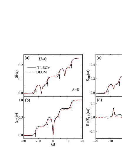
Figure 1: (Color online) The total and the lead-specified current noise spectra with noninteracting effect ($U=0$) based on TL-EOM method (black-solid line) and exact DEOM theory (red-dash line). (a) The total current noise spectrum, $S(\omega)$. (b) The central current fluctuation spectrum, $S_{\rm c}(\omega)$. (c) The auto-correlation noise spectrum of $R$-lead, $S_{\rm RR}(\omega)$. (d) The cross-correlation noise spectrum, ${\rm Re}[S_{\rm LR}(\omega)]$. The other parameters (in unit of $\Gamma$) are $\Omega=4$ and $eV=16$.

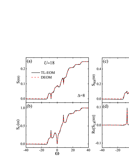
Figure 2: (Color online) The total and the lead-specified current noise spectra with with strong inter-dot Coulomb interaction ($U=18\Gamma$) based on TL-EOM method (black-solid line) and exact DEOM theory (red-dash line). (a) The total current noise spectrum, $S(\omega)$. (b) The central current fluctuation spectrum, $S_{\rm c}(\omega)$. (c) The auto-correlation noise spectrum of $R$-lead, $S_{\rm RR}(\omega)$. (d) The cross-correlation noise spectrum, ${\rm Re}[S_{\rm LR}(\omega)]$. The other parameters are the same as in Fig. 1.

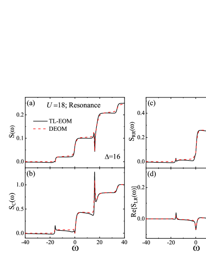
Figure 3: (Color online) The total and the lead-specified current noise spectra at resonance regime ($\varepsilon_{\pm}=\pm\Omega=\pm 8\Gamma=\pm eV/2$) with strong inter-dot Coulomb interaction ($U=18\Gamma$), based on TL-EOM method (black-solid line) and exact DEOM theory (red-dash line). (a) The total current noise spectrum, $S(\omega)$. (b) The central current fluctuation spectrum, $S_{\rm c}(\omega)$. (c) The auto-correlation noise spectrum of $R$-lead, $S_{\rm RR}(\omega)$. (d) The cross-correlation noise spectrum, ${\rm Re}[S_{\rm LR}(\omega)]$. The other parameters are the same as in Fig. 1.

The numerical results of the total and the lead-specified current noise spectra are displayed in Figs. 1, 2 and 3. They correspond to noninteracting ($U=0$), strong inter-dot interacting ($U=18\Gamma$), and the resonance regime ($U=18\Gamma$ and $\varepsilon_{+/-}=\mu_{\rm L/R}$), respectively. Furthermore, the evaluations are based on the present TL-EOM method (black solid-line) and the exact DEOM theory (red dash-line). Evidently, the TL-EOM method reproduces well, at least qualitatively, all the basic features of the quantum noise spectra in the entire frequency range. The detail demonstrations see below.

Figures 1 depicts the noise spectra in the absence of the inter-dot Coulomb interaction ($U=0$). The characteristics are as follow: (i) The well–known quasi-steps around the energy resonances, $\omega=\pm\omega_{\alpha\pm}\equiv\pm|\varepsilon_{\pm}-\mu_{\alpha}|$, emerge in the total noise spectrum $S(\omega)$, the displacement $S_{c}(\omega)$ and the diagonal component, exemplified with $S_{\rm RR}(\omega)$; see the arrows in Fig. 1(a)–(c). The aforementioned feature arises from the non-Markovian dynamics of the electrons in $\alpha$–electrode tunneling into and out of the DQDs, accompanied by energy absorption ($\omega>0$) and emission ($\omega<0$), respectively. (ii) In addition, the Rabi resonance at $\omega=\pm\Delta\equiv\pm(\varepsilon_{+}-\varepsilon_{-})$ appears in $S(\omega)$ [Fig. 1(a)] and $S_{\rm RR}(\omega)$ [Fig. 1(c)] as dips, whereas in ${\rm Re}[S_{\rm LR}(\omega)]$ [Fig. 1(d)] as peaks. On the other hand, in $S_{\rm c}(\omega)$, the former aforementioned dips and peaks are accidently canceled out [see Fig. 1(b)], in the absence of Coulomb interaction ($U=0$).

Figure 2 depicts the noise spectra in the presence of strong inter-dot Coulomb interaction ($U=18\Gamma$). (iii) In contrast to Fig. 1(b), now the displacement current noise spectrum $S_{\rm c}(\omega)$ displays at $\omega=\pm\Delta$ the Rabi coherence [see Fig. 2(b)]. While the Rabi peaks are enhanced in ${\rm Re}[S_{\rm LR}(\omega)]$ [see Fig. 2(d)], the original Rabi dips in Fig. 1(c) become peak-dip profile in $S_{\rm RR}(\omega)$ [see Fig. 2(c)]. (iv) Moreover, the Coulomb-assisted transport channels ($\varepsilon_{\pm}+U$) produces new non-Markovian quasi-steps around $\omega=\pm\omega_{\alpha{\rm u}\pm}\equiv\pm|\varepsilon_{\pm}+U-\mu_{\alpha}|$ in the total, displacement, and the auto-correlation current noise spectra, as shown in Fig. 2(a)–(c).

In Fig. 3, we highlight the characteristics of the noise spectra in the resonance regime ($\varepsilon_{+/-}=\mu_{\rm L/R}$) by increasing the coherent coupling strength $\Omega$. (v) Compared with Fig. 2, the Rabi signal in the absorption noise spectrum at $\omega=\Delta$ is remarkably enhanced, while the signal in the emission one at $\omega=-\Delta$ is negligibly small. The observation here had been explored in the isolation of competing mechanisms, such as the Kondo resonance emission noise spectrum Bas12046802 ; Del18041412 ; Mao21014104 .

The above absorptive versus emissive feature can be understood in terms of steady occupation from the following two aspects: (1) Away from the energy resonance ($\mu_{\rm L}>\varepsilon_{\pm}>\mu_{\rm R}$), the probabilities of single-electron occupied states are nearly the same, $\bar{\rho}_{++}\cong\bar{\rho}_{--}$. The resulting energy absorption and emission are equivalent in the noise spectrum. (2) In the energy resonance ($\varepsilon_{+/-}=\mu_{\rm L/R}$) region, the stationary state is very different. The lower energy state occupation on $|-\rangle$ is the majority, e.g., $\bar{\rho}_{--}\gg\bar{\rho}_{++}$. Thus, the Rabi feature in absorption is much stronger than that in emission noise.

V Summary

In summary, we have presented an efficient TL-EOM approach for the quantum noise spectrum of the transport current through interacting mesoscopic systems. The established method is based on the transformation of the second-order non-Markovian master equation described by TNL-EM into the energy-dispersed TL-EOM formalism by introducing the current-related density operator. The resulted analytical formula of the current noise spectrum can characterize the nonequilibrium transport including electron-electron Coulomb interaction and the memory effect.

We have demonstrated the proposed method in transport through interacting-quantum-dots system, and find good agreement with the exact results under broad range of parameters. The numerical calculations are based on both the present TL-EOM method and exact DEOM theory. We find that all the basic features of the lead-specified noise spectra in the entire frequency range, including energy-resonance and Coulomb-assisted non-Markovian quasi-steps, and the intrinsic coherent Rabi signal, at least qualitatively, are reconciled well with the accurate results. As a perturbative theory, the present TL-EOM is applicable in the weak system-reservoir coupling ($\Gamma\lesssim k_{\rm B}T$) regime, dominated by sequential tunneling processes. Other parameters such as the bias voltage and Coulomb interaction, are rather flexible.

Appendix A Derivation of the noise spectrum

In this appendix, we first give the derivation for the current correlation function Eq. (23) and then its Laplace transformation resulting in the current noise spectrum formula Eq. (III.3). The details are below.

In the current correlation function expressed by Eq. (20), one needs to get the solution of $\rho^{\sigma}_{\alpha u}(E,t;\alpha^{\prime})$. Based on Eq. (9b) with the initial condition of Eq. (19b), we have

$$\rho^{\sigma}_{\alpha u}(E,t;\alpha^{\prime})=-i\,\delta_{\alpha\alpha^{\prime}}e^{-i({\cal L}_{\mbox{\tiny S}}-\sigma E)t}\!\sum_{v}\Gamma^{\sigma}_{\alpha uv}(E)\tilde{a}^{\sigma}_{v}\bar{\rho}$$

$$\quad\quad-i\int_{0}^{t}\!\!{\mathrm{d}}\tau e^{-i({\cal L}_{\mbox{\tiny S}}-\sigma E)(t-\tau)}{\cal C}^{\sigma}_{\alpha u}(E)\rho(\tau;\alpha^{\prime}).$$ (36)

This straightforwardly recasts Eq. (20) to Eq. (23).

Next, we are going to get the current noise spectrum formula Eq. (III.3), according to the definition of Eq. (21). Following the procedure of Refs. Yan14054105 ; Jin15234108 ; Yan16110306 , the quantum noise spectrum can be calculated via

$$S_{\alpha\alpha^{\prime}}(\omega)={\cal I}_{\alpha\alpha^{\prime}}(\omega)+{\cal I}^{\ast}_{\alpha^{\prime}\alpha}(\omega),$$ (37)

with the introduction of

$${\cal I}_{\alpha\alpha^{\prime}}(\omega)\equiv\int_{0}^{\infty}\!dt\,e^{i\omega t}\langle{\hat{I}}_{\alpha}(t){\hat{I}}_{\alpha^{\prime}}(0)\rangle\,.$$ (38)

In terms of the steady current correlation function given by Eq. (23), we can straightforwardly have,

$${\cal I}_{\alpha\alpha^{\prime}}(\omega) =\delta_{\alpha^{\prime}\alpha}\sum_{\sigma uv}{\rm tr}_{\rm s}\big{[}a^{\bar{\sigma}}_{u}C^{(\sigma)}_{\alpha uv}(\omega-{\cal L})a^{\sigma}_{v}{\bar{\rho}}\big{]}$$

$$\quad+{\rm tr}_{\rm s}\big{[}{\cal J}^{>}_{\alpha}(\omega)\rho(\omega;\alpha^{\prime})\big{]},$$ (39a)

$${\cal I}^{\ast}_{\alpha^{\prime}\alpha}(\omega) =\delta_{\alpha^{\prime}\alpha}\sum_{\sigma uv}{\rm tr}_{\rm s}\big{[}C^{(\bar{\sigma})\ast}_{\alpha uv}(\omega+{\cal L})\bar{\rho}a^{\sigma}_{v}a^{\bar{\sigma}}_{u}\big{]}$$

$$\quad+{\rm tr}_{\rm s}\big{[}{\cal J}^{<}_{\alpha^{\prime}}(-\omega)\rho^{\dagger}(\omega;\alpha)\big{]},$$ (39b)

where ${\cal J}^{\mbox{\tiny$\lessgtr$}}(\omega)$ is defined in Eq. (25), and $C^{(\pm)}_{\alpha uv}(\omega)=\int^{\infty}_{0}dt\,e^{i\omega t}C^{(\pm)}_{\alpha uv}(t)$ is obtained as Jin14244111 ; Shi16095002 ; Jin16083038

$$C^{(\pm)}_{\alpha uv}(\omega)=\frac{1}{2}\big{[}\Gamma^{(\pm)}_{\alpha uv}(\mp\omega)+i\Lambda^{(\pm)}_{\alpha uv}(\mp\omega)\big{]}.$$ (40)

The real [c.f.Eq. (4)] and the imaginary parts are the so-called bath interaction spectrum and dispersion, respectively Xu029196 . They are related via the Kramers-Kronig relations:

$$\Lambda^{(\pm)}_{\alpha uv}(\omega) ={\cal P}\int^{\infty}_{-\infty}\frac{{\mathrm{d}}\omega^{\prime}}{2\pi}\frac{1}{\omega\pm\omega^{\prime}}\Gamma^{(\pm)}_{\alpha uv}(\omega)$$

$$=\frac{\Gamma_{\alpha uv}(\omega)}{2\pi}\Bigg{\{}{\rm Re}\left[\Psi\left(\frac{1}{2}+i\frac{\beta(\omega-\mu_{\alpha})}{2\pi}\right)\right]$$

$$\quad-\Psi\left(\frac{1}{2}+\frac{\beta W_{\alpha}}{2\pi}\right)\mp\pi\frac{\omega-\mu_{\alpha}}{W_{\alpha}}\Bigg{\}},$$ (41)

where ${\cal P}$ denotes the principle value of the integral, and $\Psi(x)$ is the digamma function. In Eq. (A), the second identity is from the consideration of the Lorentzian-type form of the hybridization spectral density, i.e.,

$$J_{\alpha uv}(\omega)=\frac{\Gamma_{\alpha uv}W^{2}_{\alpha}}{(\omega-\mu_{\alpha})^{2}+W^{2}_{\alpha}},$$ (42)

with the coupling strength $\Gamma_{\alpha uv}$ and the bandwidth $W_{\alpha}$ of lead-$\alpha$.

In Eq. (39), the key is to get the solutions of $\rho(\omega;\alpha^{\prime})$ and $\rho^{\dagger}(\omega;\alpha)$. Setting $\dot{\rho}^{\sigma}_{\alpha u}(E,t)=0$ in Eq. (9b), we first get the stationary solution of

$$\bar{\rho}^{\sigma}_{\alpha u}(E)=\frac{\sum_{v}\big{[}\Gamma^{\sigma}_{\alpha uv}(E)a^{\sigma}_{v}\bar{\rho}-\Gamma^{{\bar{\sigma}}\ast}_{\alpha uv}(E)\bar{\rho}a^{\sigma}_{v}\big{]}}{\sigma E-{\cal L}_{\mbox{\tiny S}}+i0^{+}}.$$ (43)

Inserting it into Eq. (19a), we have

$$\rho(0;\alpha^{\prime}) =\!-\!\sum_{\sigma u}\tilde{a}^{\bar{\sigma}}_{u}{\cal C}^{(\sigma)}_{\alpha^{\prime}u}(-{\cal L}_{\mbox{\tiny S}})\bar{\rho}={\cal J}^{>}_{\alpha^{\prime}}(0)\bar{\rho}.$$ (44)

Now $\rho(\omega;\alpha^{\prime})=\int_{0}^{\infty}{\rm d}te^{i\omega t}\rho(t;\alpha^{\prime})$ can then be obtained by either TNL-ME (6) with the initial condition of Eq. (44) or by TL-EOM (9) with ${\bm{\rho}}(0;\alpha^{\prime})$ described by Eq. (44) and Eq. (19b). One then can easily get

$$\rho(\omega;\alpha^{\prime}) =\Pi(\omega)\Big{\{}{\cal J}^{>}_{\alpha^{\prime}}(0)\bar{\rho}+{\cal W}^{>}_{\alpha^{\prime}}(\omega)\bar{\rho}\Big{\}}.$$ (45)

Further with the relation of Eq. (28), we obtain

$$\rho^{\dagger}(\omega;\alpha) =\Pi(-\omega)\Big{\{}{\cal J}^{<}_{\alpha}(0)\bar{\rho}+{\cal W}^{<}_{\alpha}(-\omega)\bar{\rho}\Big{\}}.$$ (46)

Finally, based on Eq. (37) to Eq. (39), the general lead-specified formula of quantum noise spectrum, Eq. (III.3), is straightforwardly obtained.

References

- (1) Y. M. Blanter and M. Büttiker, Phys. Rep. 336, 1 (2000).
- (2) I. Imry, Introduction to Mesoscopic Physics, Oxford university press, 2002.
- (3) C. Beenakker and C. Schnenberger, Phys. Today 56, 37 (2003).
- (4) Quantum Noise in Mesoscopic Physics, Kluwer, Dordrecht, 2003, edited by Y. V. Nazarov.
- (5) R. Deblock, E. Onac, L. Gurevich, and L. P. Kouwenhoven, Science 301, 203 (2003).
- (6) Delattre et al., Nature Physics 5, 208 (2009).
- (7) J. Basset, H. Bouchiat, and R. Deblock, Phys. Rev. Lett. 105, 166801 (2010).
- (8) J. Basset et al., Phys. Rev. Lett. 108, 046802 (2012).
- (9) R. Delagrange, J. Basset, H. Bouchiat, and R. Deblock, Phys. Rev. B 97, 041412 (2018).
- (10) H.-A. Engel and D. Loss, Phys. Rev. Lett. 93, 136602 (2004).
- (11) R. Aguado and L. P. Kouwenhoven, Phys. Rev. Lett. 84, 1986 (2000).
- (12) K. Nakata, Y. Ohnuma, and M. Matsuo, Phys. Rev. B 99, 134403 (2019).
- (13) O. Entin-Wohlman, Y. Imry, S. A. Gurvitz, and A. Aharony, Phys. Rev. B 75, 193308 (2007).
- (14) E. A. Rothstein, O. Entin-Wohlman, and A. Aharony, Phys. Rev. B 79, 075307 (2009).
- (15) H. Mao, J. Jin, S. Wang, and Y. Yan, J. Chem. Phys. 155, 014104 (2021).
- (16) J. S. Jin, X. Zheng, and Y. J. Yan, J. Chem. Phys. 128, 234703 (2008).
- (17) X. Zheng, J. S. Jin, S. Welack, M. Luo, and Y. J. Yan, J. Chem. Phys. 130, 164708 (2009).
- (18) Z. H. Li, N. H. Tong, X. Zheng, D. Hou, J. H. Wei, J. Hu, and Y. J. Yan, Phys. Rev. Lett. 109, 266403 (2012).
- (19) S. K. Wang, X. Zheng, J. S. Jin, and Y. J. Yan, Phys. Rev. B 88, 035129 (2013).
- (20) Y. X. Cheng, W. J. Hou, Y. D. Wang, Z. H Li, J. H. Wei, and Y. J. Yan, New J. Phys. 17, 033009 (2015).
- (21) Y. J. Yan, J. Chem. Phys. 140, 054105 (2014).
- (22) J. S. Jin, S. K. Wang, X. Zheng, and Y. J. Yan, J. Chem. Phys. 142, 234108 (2015).
- (23) Y. J. Yan, J. S. Jin, R. X. Xu, and X. Zheng, Frontiers Phys. 11, 110306 (2016).
- (24) J. S. Jin, Phys. Rev. B 101, 235144 (2020).
- (25) M. W. Y. Tu and W.-M. Zhang, Phys. Rev. B 78, 235311 (2008).
- (26) J. S. Jin, M. W.-Y. Tu, W.-M. Zhang, and Y. J. Yan, New J. Phys. 12, 083013 (2010).
- (27) P.-Y. Yang, C.-Y. Lin, and W.-M. Zhang, Phys. Rev. B 89, 115411 (2014).
- (28) J. S. Jin, C. Karlewski, and M. Marthaler, New J. Phys. 18, 083038 (2016).
- (29) J. S. Jin, X. Q. Li, M. Luo, and Y. J. Yan, J. Appl. Phys. 109, 053704 (2011).
- (30) B. Wang, J. Wang, and H. Guo, Phys. Rev. Lett. 82, 398 (1999).
- (31) D. Marcos, C. Emary, T. Brandes, and R. Aguado, New Journal of Physics 12, 123009 (2010).
- (32) R. X. Xu, Y. J. Yan, and X. Q. Li, Phys. Rev. A 65, 023807 (2002).
- (33) X. Q. Li, W. K. Zhang, P. Cui, J. S. Shao, Z. S. Ma, and Y. J. Yan Phys. Rev. B 69, 085315 (2004).
- (34) X. Q. Li, J. Y. Luo, Y. G. Yang, P. Cui, and Y. J. Yan, Phys. Rev. B 71, 205304 (2005).
- (35) X. Q. Li, P. Cui, and Y. J. Yan, Phys. Rev. Lett. 94, 066803 (2005).
- (36) J. Y. Luo, X. Q. Li, and Y. J. Yan, Phys. Rev. B 76, 085325 (2007).
- (37) R. Aguado and T. Brandes, Phys. Rev. Lett. 92, 206601 (2004).
- (38) D. Marcos, C. Emary, T. Brandes, and R. Aguado, Phys. Rev. B 83, 125426 (2011).
- (39) P. Shi, M. Hu, Y. Ying, and J. Jin, AIP ADVANCES 6, 095002 (2016).
- (40) J. S. Jin, J. Li, Y. Liu, X.-Q. Li, and Y. J. Yan, J. Chem. Phys. 140, 244111 (2014).
- (41) R. X. Xu and Y. J. Yan, J. Chem. Phys. 116, 9196 (2002).