Incentive-compatible public transportation fares with random inspection

Abstract.

We consider the problem of designing prices for public transport where payment enforcing is done through random inspection of passengers’ tickets as opposed to physically blocking their access. Passengers are fully strategic such that they may choose different routes or buy partial tickets in their optimizing decision. We derive expressions for the prices that make every passenger choose to buy the full ticket. Using travel and pricing data from the Washington DC metro, we show that a switch to a random inspection method for ticketing while keeping current prices could lead to more than 59% of revenue loss due to fare evasion, while adjusting prices to take incentives into consideration would reduce that loss to less than 20%, without any increase in prices.

1. Introduction

In many, if not most, cities in the world, passengers using public transportation have their access to bus and rail systems controlled by barriers that can only be passed by making cash payments, inserting a ticket or tapping a card or a cellphone. In most cities in Germany, the Netherlands, Italy, among others, a proof-of-payment system is used instead. In these systems, the public have unrestricted access to buses and trains, but are expected to buy the tickets that correspond to their travel. The enforcement of these purchases is done by inspectors, who perform random checks of passengers during their trips. If they are not carrying the correct ticket for their trip, they receive a fine.

Transport networks that use proof-of-payment systems require a much simpler infrastructure at stations and buses: subway stations can be directly connected to the streets, trams can stop at arbitrary locations, and bus drivers do not have to handle passenger payments or ticketing. The downside, however, is that it is much easier for passengers to ride without paying. This, of course, can have a potentially catastrophic impact on revenue.

In this paper, we consider the problem of setting prices for proof-of-payment public transportation systems when passengers act as self-interested strategic agents, choosing the tickets they buy and the routes they take to minimize the expected cost of their trip. We derive the expressions for the incentive-compatible prices, i.e., the prices such that passengers will choose to buy the correct ticket for their trip, for both a stylized in a line and for an arbitrary network.

Given these expressions, we use real-life network and passenger travel data for the Washington D.C. metro to derive the incentive-compatible prices that result from our model. These show that, for the most part, the dollar values that result from the direct application of our expressions seem reasonably applicable. We then simulate the scenario in which the Washington D.C. metro switches to a proof-of-payment system without changing the pricing structure. These indicate that fare evasion by strategic passengers could lead to a revenue loss of more than 59%. An adjustment to the D.C. prices to make them incentive compatible, despite making them weakly lower across the board, would reduce the revenue loss to less than 20% instead, indicating that incentive considerations can have a substantial impact.

2. Related literature

Our paper contributes to a voluminous literature on payment evasion: shoplifting (Yaniv, 2009; Perlman and Ozinci, 2014), digital piracy (Chellappa and Shivendu, 2005), tax evasion (Slemrod, 2007), parking violations (Fisman and Miguel, 2007), and public transportation fare evasion (Boyd et al., 1989; Kooreman, 1993), and monitoring and punishment. Becker (1968) shows that maximal fine is the optimal because it does not distort incentive. Subsequent literature suggest, however, that the maximal fine may not be optimal under different extensions (Polinsky and Shavell, 1979, 1984, 2000; Malik, 1990). Our analysis also relates to the operation research literature on fare inspection in the network (Yin et al., 2012), network security game (Jain et al., 2013), and fare collection systems (Tirachini and Hensher, 2012).

Correa et al. (2017) is the closest to our paper. In it, passengers act strategically, being able to buy or not a ticket based on the expected value of each strategy, and the transport agency optimizes the location of the inspectors. Their focus is on producing and evaluating the complexity of algorithms for determining the optimal positioning of inspectors in the network. They also consider an extension in which the prices considers the possibility that a passenger can choose not to buy the ticket. Among other differences, in their model the probability of a passenger being inspected is independent of the number of passengers who choose travel through the same segment.

3. Baseline model

There is a positive mass of passengers residing in a line $[0,1]$. Denote $\mathcal{I}$ the set of passengers. Passengers have travel demand density $d\left(x,y\right)$, where $x$ is the origin and $y$ the destination. The function $d$ is continuously differentiable, and we have $d\left(x,y\right)>0$ for any $x,y\in[0,1]$ and $x\neq y$. As an illustration, $\int_{0}^{1}d\left(0,x\right)dx$ is the mass of passengers who wants to travel from point 0.

An important measure, for our purposes, is the density function that tells the mass of passengers that wants to pass through a point $a$ (that is, passengers who start at or before $a$ and leave at or after $a$). This function, $d^{pass}$, can therefore be defined by:

$$d^{pass}\left(a\right)=\int_{0}^{a}\int_{a}^{1}d\left(x,y\right)dy\ dx+\int_{a}^{1}\int_{0}^{a}d\left(x,y\right)dy\ dx$$

The first part consists of all passengers who depart from some point in $[0,a]$ and go to some point in $[a,1]$. The second part consists of all passengers who depart from some point in $[a,1]$ and go to some point in $[0,a]$.

There is a pricing scheme $p$ for every pair of origin and destination. Any tickets can be purchased at every point of departure, at a price $p\left(x,y\right)$, where $x$ is the origin and $y$ the destination.

A passenger who demands to make a trip have to make the full trip. She is free, however, to choose any path between her origin and destination, and to buy any set of tickets, if any, she wants for that trip. Hence, her strategy consists of the combination of (i) a path from her origin to her destination, and (ii) a set of tickets (if any). Formally, a strategy for passenger $i\in\mathcal{I}$, who resides at point $x_{i}$ and has as destination point $y_{i}$, is a pair $s_{i}=(\sigma_{i},\tau_{i})$, where $\sigma_{i}=\left(x_{i},\sigma_{i}^{0},\sigma_{i}^{1},\ldots,y_{i}\right)$ is the path that the passenger follows: starting from $x_{i}$, goes to $\sigma_{i}^{0}$, then $\sigma_{i}^{1}$, etc, ending at her destination $y_{i}$. The set $\tau_{i}=\left\{(\tau_{i}^{0},\tau_{i}^{1}),(\tau_{i}^{2},\tau_{i}^{3}),\ldots,(\tau_{i}^{k-1},\tau_{i}^{k})\right\}$ are the tickets that the passenger $i$ purchases—for example, one ticket from $\tau_{i}^{0}$ to $\tau_{i}^{1}$.

To reduce fare evasion, the transportation authority has a mass $\lambda^{total}$ of inspectors, and distributes them along the line. Without loss of generality, we normalize the mass to unity, i.e., $\lambda^{total}=1$ so that we can describe the distribution of inspectors with a probability density function $\lambda\left(x\right)$. The probability that a passenger is inspected when traveling between $x$ and $y$, is given by the following expression:

$$q\left(x,y,\lambda\right)=\left|\int_{x}^{y}\frac{\phi\left(\lambda\left(a\right)\right)}{d^{pass}\left(x\right)}da\right|$$

where $\phi$ is a monotonically increasing and quasi-concave function of the mass of inspectors. The case $\phi\left(x\right)=x$, for example, represents the case in which the probability of being inspected equals the ratio of inspectors to passengers. Note that $q$ is symmetric in the first two arguments, so that $q(x,y,\lambda)=q(y,x,\lambda)$.

If a passenger is inspected at any point $a\in[0,1]$ and does not have a ticket, she receives a fine of $\alpha$. Moreover, if she has a ticket with origin-destination $(x,y)$ but either $a<x$ or $a>y$, then she is also punished with the same fine. While we will make considerations about how the transportation authority would distribute the inspectors, we assume that it does not incorporate revenues from fines.

We assume that passengers have quasi-linear utilities, are risk neutral and maximize expected utility. Passenger $i\in\mathcal{I}$ derives utility $u_{i}\left(x,y\right)$ from making a trip from $x$ to $y$. The (expected) utility that the passenger $i$ who travels from $x$ to $y$ derives from her strategy $s_{i}=(\sigma_{i},\tau_{i})$ is:

$$u_{i}\left(x,y\right)-\alpha\sum_{(a,b)\in\sigma_{i}\backslash\tau_{i}}q(a,b,\lambda)-\sum_{(a,b)\in\tau_{i}}p\left(a,b\right)$$

where the second term is the expected payment of fine if being inspected on the line segment without ticket and the third term is the total cost of tickets purchased.

Under pricing scheme $p$, the strategy profile $s=(s_{i})_{i\in\mathcal{I}}=(\sigma_{i},\tau_{i})_{i\in\mathcal{I}}$ is an equilibrium if no passenger can be strictly better off by unilaterally deviating to another strategy. A pricing scheme is incentive-compatible if there is an equilibrium such that all passengers buy full tickets corresponding to their trip.

Under strategy profile $s$, the total revenue of the transportation authority is given by:

$$\pi(p,s)=\sum_{(x,y)\subseteq[0,1]^{2}}p\left(x,y\right)\left|\{i\in\mathcal{I}:(x,y)\in\tau_{i}\}\right|$$

where $\left|\{i\in\mathcal{I}:(x,y)\in\tau_{i}\}\right|$ is the mass of passengers who buy tickets between $x$ and $y$. A pricing scheme $p^{*}$ is revenue-maximizing if it maximizes total revenue $\pi(p^{*},s^{*})$ where $s^{*}$ is an equilibrium under $p^{*}$.

Passengers have the reservation values of riding without buying any ticket. Therefore, the maximum surplus that can be extracted from a passenger $i$ with demand for travel from $x$ to $y$ is $u_{i}\left(x,y\right)-\alpha q(x,y,\lambda)$. Hence, a pricing scheme $p^{*}$ is full-surplus-extracting if it is incentive-compatible and every passenger $i\in\mathcal{I}$ has payoff $u_{i}\left(x,y\right)-\alpha q(x,y,\lambda)$ in an equilibrium $s^{*}$ under $p^{*}$. Note that if is a pricing scheme is full-surplus-extracting, then it is also revenue-maximizing.

Our first result is to show that there is incentive-compatible pricing scheme, and that this pricing scheme extracts all the surplus from passengers and thus also maximizes the revenue for the transportation authority.

Proposition 1.

The pricing scheme $p^{*}\left(x,y\right)=\alpha q(x,y,\lambda)$ is incentive-compatible, full-surplus extracting and revenue-maximizing.

Proof.

Consider a passenger $i$ who needs to make a trip from $x$ to $y$ under the pricing scheme $p^{*}$. Without loss of generality assume $x<y$. First, suppose a passenger $i$ is buying the full ticket from $x$ to $y$ , i.e., $\sigma_{i}=\tau_{i}$. Since $p^{*}$ is increasing for a larger line segment (in the sense of inclusion), it suffices to consider $\sigma_{i}=(x,y)$. The utility of this passenger is

$$U^{Full}_{i}(x,y)\equiv u_{i}\left(x,y\right)-p^{*}(x,y)=u_{i}\left(x,y\right)-\alpha q(x,y,\lambda)$$

Second, consider the passenger $i$ is not buying any single ticket. The utility is

$$U^{None}_{i}(x,y)\equiv u_{i}\left(x,y\right)-\alpha q(x,y,\lambda)$$

which is the minimum utility that the passenger can get, since there is always a option to travel without buying a ticket. Hence, as $U^{Full}_{i}(x,y)=U^{None}_{i}(x,y)$, the passenger $i$ is indifferent between buying the full ticket and buying no ticket.

Now consider a passenger $i$ who buys a subset of tickets, i.e., using a strategy such that $\sigma_{i}\neq\tau_{i}$. By the monotonicity of price $p^{*}$, it is strictly dominated to buy tickets outside line segments between $x$ and $y$ and also dominated to buy overlapping line segments. Hence, we only need to consider tickets covering disjoint segments between $x$ and $y$. Formally, passenger $i$ buys $n$ tickets where the $i$-th ticket covers the segment $(a_{i},b_{i})$ where $a_{1}\leq b_{1}\leq a_{2}\leq b_{2}\leq\ldots\leq a_{n}\leq b_{n}$. where $x\leq a_{1}$ and $b_{n}\leq y$. The utility is

$$U^{Partial}_{i}(s_{i},x,y) \equiv u_{i}\left(x,y\right)-\alpha\sum_{(a,b)\in\sigma_{i}\backslash\tau_{i}}q(a,b,\lambda)-\sum_{(a,b)\in\tau_{i}}p^{*}(a,b)$$

$$=u_{i}\left(x,y\right)-\alpha\sum_{(a,b)\in\sigma_{i}\backslash\tau_{i}}q(a,b,\lambda)-\alpha\sum_{(a,b)\in\tau_{i}}q(a,b,\lambda)$$

$$=u_{i}\left(x,y\right)-\alpha q(x,y,\lambda).$$

Hence, we have $U^{Full}_{i}(x,y)=U^{None}_{i}(x,y)=U^{Partial}_{i}(s_{i},x,y)$ for all strategies $s_{i}$ and this equality holds for all possible origin $x$ and destination $y$. This implies that all passengers are indifferent between any tickets purchase (including no ticket at all).

Any price above $p^{*}\left(x,y\right)$ will make the passenger ride without paying. Therefore: (i) all surplus is extracted under $p^{*}\left(x,y\right)$, (ii) revenue is maximal, and (iii) every passenger buys tickets between $x$ and $y$ for every $p^{\prime}(x,y)\leq p^{*}\left(x,y\right)$. ∎

Next, we consider the distribution of inspectors $\lambda$. The focus of this paper are the prices and the incentives that they induce on strategic passengers, and therefore we have taken the distribution of inspectors as given. However, understanding what would be the “optimal” choice for that distribution is important if we want to understand whether the scenarios that we will consider can be deemed as reasonable.

A distribution of inspector $\lambda$ is revenue-maximizing if it maximizes the revenues of a transportation authority under some revenue-maximizing pricing scheme.. The following shows the revenue-maximizing inspector distribution is rather simple.

Proposition 2.

The distribution of inspectors $\lambda$ is revenue-maximizing if, for any two points $x,y\in[0,1]$,

$$\phi^{\prime}\left(\lambda\left(x\right)\right)=\phi^{\prime}\left(\lambda\left(y\right)\right).$$

Proof.

From Proposition 1, a revenue-maximizing price is also incentive-compatible. Hence, under this price $p^{*}$, the profit of transportation authority is

$$\pi=\int_{0}^{1}\int_{x}^{1}d(x,y)p^{*}(x,y)dy\ dx+\int_{0}^{1}\int_{0}^{x}d(x,y)p^{*}(x,y)dy\ dx$$

Since $p^{*}(x,y)=\alpha q(x,y,\lambda)=\alpha\left|\int_{x}^{y}\frac{\phi\left(\lambda\left(a\right)\right)}{d^{pass}\left(a\right)}da\right|$, we have

$$\pi=\alpha\int_{0}^{1}\int_{x}^{1}d(x,y)\left[\int_{x}^{y}\frac{\phi\left(\lambda\left(a\right)\right)}{d^{pass}\left(a\right)}da\right]dy\ dx+\alpha\int_{0}^{1}\int_{0}^{x}d(x,y)\left[\int_{x}^{y}\frac{\phi\left(\lambda\left(a\right)\right)}{d^{pass}\left(a\right)}da\right]dy\ dx$$

By changing the order of integration, we have

$$\pi=\alpha\int_{0}^{1}\int_{0}^{a}\int_{a}^{1}\left[d(x,y)\frac{\phi\left(\lambda\left(a\right)\right)}{d^{pass}\left(a\right)}\right]dy\ dx\ da+\alpha\int_{0}^{1}\int_{a}^{1}\int_{0}^{a}\left[d(x,y)\frac{\phi\left(\lambda\left(a\right)\right)}{d^{pass}\left(a\right)}\right]dy\ dx\ da$$

The distribution of inspectors is such that the following holds:

$$\int_{0}^{1}\lambda(x)dx=1.$$

Hence, we have the Lagrangian:

$$\mathcal{L}=\pi+\Lambda\left[1-\int_{0}^{1}\lambda(x)dx\right]$$

where $\Lambda$ is the Lagrangian multiplier. The FOCs on the Lagrangian are:

$$\frac{\partial\mathcal{L}}{\partial\lambda(a)}=0\text{ for all }a\in[0,1]\text{ and }\int_{0}^{1}\lambda(x)dx=1.$$

The first set of equations implies that we have

$$\alpha\int_{0}^{a}\int_{a}^{1}\left[d(x,y)\frac{\phi^{\prime}\left(\lambda\left(a\right)\right)}{d^{pass}\left(a\right)}\right]dy\ dx+\alpha\int_{a}^{1}\int_{0}^{a}\left[d(x,y)\frac{\phi^{\prime}\left(\lambda\left(a\right)\right)}{d^{pass}\left(a\right)}\right]dy\ dx=\Lambda$$

The expression $\frac{\phi^{\prime}\left(\lambda\left(a\right)\right)}{d^{pass}\left(a\right)}$ is independent of $x$ and $y$, and therefore we can rearrange as

$$\frac{\phi^{\prime}\left(\lambda\left(a\right)\right)}{d^{pass}\left(a\right)}\alpha\left[\int_{0}^{a}\int_{a}^{1}d(x,y)dy\ dx+\int_{a}^{1}\int_{0}^{a}d(x,y)dy\ dx\right]=\Lambda$$

Since $d^{pass}(a)=\int_{0}^{a}\int_{a}^{1}d(x,y)dy\ dx+\int_{a}^{1}\int_{0}^{a}d(x,y)dy\ dx$, we have

$$\phi^{\prime}\left(\lambda\left(a\right)\right)\alpha=\Lambda,$$

for all $a\in[0,1]$. Thus, we have for any two points $x,y\in[0,1]$,

$$\phi^{\prime}\left(\lambda\left(x\right)\right)=\phi^{\prime}\left(\lambda\left(y\right)\right)=\Lambda/\alpha.$$

∎

Proposition 2 results in two important corollaries:

Corollary 1.

If $\phi$ is strictly concave, the revenue-maximizing distribution of inspectors $\lambda^{*}$ is such that for every $i,j$, $\lambda^{*}(i)=\lambda^{*}(j)$.

Corollary 2.

If $\phi(\lambda)=k\lambda$ for some constant $k>0$, then any distribution of inspectors $\lambda^{*}$ for which $\int_{0}^{1}\lambda(x)dx=1$ is revenue-equivalent.

Corollary 2 implies that if the probability of a passenger being inspected is proportional to the probability that an individual in a train is an inspector, revenue maximization does not imply in a restriction on the distribution of inspectors.

4. Networks

In this section, we consider a model in which space is not a line segment, but an arbitrary discrete network. Passengers travel from an two different nodes in the network, and they can only travel through the edges that connect them. A network is a set of nodes $\mathcal{N}=\{N_{1},N_{2},N_{3},\ldots\}$ and of edges $\mathcal{E}$, which is a collection of pairs of nodes. For each origin $x\in\mathcal{N}$ and destination $y\in\mathcal{N}$, there is an exogenous demand $D_{(x,y)}>0$, that gives the mass of passengers who want to travel from $x$ to $y$. Denote $\mathcal{D}=\left(D_{(x,y)}\right)_{(x,y)\in\mathcal{N}^{2}}$ the set of demands for all origin and destination. Each passenger $i$ derives utility $u_{i}(x,y)$ from his trip.

Passengers now have more options than simply traveling or not: there might be multiple ways to travel between two nodes. For example, in a connected graph with three nodes $x,y,z$, a passenger who wants to go from node $x$ to node $y$ can either take the direct route, through the edge $(x,y)$, or take the indirect route through edges $(x,y)$ and then $(y,z)$.

Following Section 3, a passenger $i$’s strategy consists of the combination of (i) a path from her origin to her destination—a set of connected edges in $\mathcal{E}$—($\sigma_{i}$), and (ii) a set of tickets ($\tau_{i}$). Given strategies of all passengers, denote $\sigma^{Pass}_{(x,y)}$ be the mass of passengers that pass through the edge $(x,y)$:

$$\sigma^{Pass}_{(x,y)}=|\{i\in\mathcal{I}:(x,y)\in\sigma_{i}\}|+|\{i\in\mathcal{I}:(y,x)\in\sigma_{i}\}|.$$

Each edge $(x,y)$ is monitored by a mass $\lambda_{(x,y)}>0$ of inspectors. Normalizing the total mass of inspectors to unity, let $\lambda$ be a distribution of inspectors and there is full support over all the edges. The probability that a passenger is inspected when traveling through the edge connecting $x$ and $y$, is given by the following expression:

$$Q_{\left(x,y\right)}(\lambda)=\frac{\phi\left(\lambda_{\left(x,y\right)}\right)}{\sigma^{pass}_{\left(x,y\right)}}$$

where the first term is the mass of passengers travelling from node $x$ to $y$ and the second term is the mass of passengers travelling in the other direction.

The transportation authority sets a pricing scheme $P$ for every pair of origin and destination. Any tickets can be purchased at every point of node, at a price $P_{(x,y)}$, where $x$ is the origin and $y$ the destination.

Given the pricing scheme $P$, monitors distribution $\lambda$ and strategies from all other passengers $\sigma^{pass}_{-i}$, the expected utility that passenger $i$ who travels from $x$ to $y$ with strategy $s_{i}=(\sigma_{i},\tau_{i})$ is:

$$u_{i}\left(x,y\right)-\alpha\sum_{(a,b)\in\sigma_{i}\backslash\tau_{i}}Q_{(a,b)}(\lambda)-\sum_{(a,b)\in\tau_{i}}P_{\left(a,b\right)}$$

Under the pricing scheme $P$, the strategy profile $s=(\sigma_{i},\tau_{i})_{i\in\mathcal{I}}$ is an equilibrium if no passenger can be strictly better off by deviating to another strategy. A pricing scheme is incentive-compatible if there is an equilibrium such that every passenger buy the full ticket.

Under strategy profile $s$, the total revenue of the transportation authority is given by:

$$\pi(P,s)=\sum_{(x,y)\subseteq\mathcal{N}^{2}}P_{\left(x,y\right)}\left|\{i\in\mathcal{I}:(x,y)\in\tau_{i}\}\right|$$

where $\left|\{i\in\mathcal{I}:(x,y)\in\tau_{i}\}\right|$ is the mass of passengers who buy tickets between $x$ and $y$. A pricing scheme $P^{*}$ is revenue-maximizing if it maximizes total revenue $\pi(P^{*},s^{*})$ where $s^{*}$ is an equilibrium under $P^{*}$.

We will show that there exists a system of positive prices on every edge such that all passengers buy full tickets in equilibrium. We do so by constructing a game in which all passengers are free to choose any route between their origin and destination, but must pay full price on their trips. Moreover, in this game, as opposed to our model, prices are not given, but a function of all passengers’ route choices. We then show that under these prices all passengers will choose to buy the tickets in the original model, in which they choose the path and the tickets to purchase.

Proposition 3.

For any network $G=(\mathcal{N},\mathcal{E})$ such that demand $\mathcal{D}$ and distribution of monitors $\lambda$ have full support over all the edges, there is an incentive-compatible, revenue-maximizing pricing scheme.

Proof.

To start, we consider a modified simultaneous move game that have two changes from the original game. First, each passenger only needs to choose which path they want to follow between their origin and destination, while paying full price on their trips (that is, they are not strategic about ticket purchasing). Hence, a passenger $i$’s strategy is just a path between $x$ and $y$. Second, prices are not taken as given but endogenously determined by the combination of all passengers’ choices of paths. More specifically, we consider the price of each edge $(x,y)$ is given by

(1) $$P_{(x,y)}=\frac{\phi\left(\lambda_{(x,y)}\right)}{\sigma^{pass}_{(x,y)}}\alpha.$$

Given the price $P_{(x,y)}$, we can see that the utility is continuous on other passengers’ mixed strategies: the utility of a passenger when traveling through a path is his valuation from travel minus the sum of all $P_{(x,y)}$ along the path travelled. Since we have full support on monitoring and the number of travelers passing through each edge (since for every every edge $(x,y)$ it is the case that $D_{(x,y)}>0$, each edge is traveled, at the very least, by those who have $x$ and $y$ as their origin and destination), continuous changes in other players’ strategies change continuously the value of $\sigma^{pass}_{(x,y)}$.

We have, therefore, a continuum of players playing a game with a finite number of strategies (that are, for each player, all the paths between their origin and destination). Following Schmeidler (1973), when the payoffs of the passengers are continuous on the mixture of other passengers’ strategies, there exists a mixed strategy Nash equilibrium. Hence, we have the existence of a mixed strategy equilibrium of this modified game.

By the continuum of passengers and the law of large numbers, there is a pure strategy equilibrium where the randomization probability of a path under the mixed strategy equilibrium is the equilibrium fraction of passengers choosing that path in a pure strategy equilibrium.

Now we return to the original game where price is given from the equilibrium in the modified game. We argue that passengers would continue to travel the same path and purchase the full ticket.

First, passengers in the original game would continue to travel the same path as in the modified game. If there is a profitable deviation in the original game, then there will be also a profitable deviation in the modified game, which is a contradiction.

Second, passengers will purchase the full ticket. Since the logic is exactly the same behind the proof in Proposition 1, we only verbally describe the steps here. Note that the price between every two nodes is set to equal the expected loss of not having a buying a ticket between these two nodes. So regardless of the node of departure that is being considered (and therefore regardless of whether a ticket was purchased for the previous path), following the equilibrium path from then on both (1) minimizes the cost of being monitored without a ticket and (2) minimizes the price paid.

Finally, this pricing scheme is revenue-maximizing. Notice that a lower price at any segment will not increase participation in travels, so it will not increase revenues. Moreover, any increase for the price in a segment makes everybody travel through that segment without paying for it. So, increasing the price at any edge also reduces revenue. ∎

5. Application: the Washington DC Metro

In this last section, we use traffic and pricing data from the Washington DC metro system as an example of the impact that our incentive-compatible pricing scheme could have in a real-life public transport system. Our objective is, first, to see whether given actual values for traffic between stations and realistic numbers for the number of inspectors, the values for the punishment fee $\alpha$ and for the incentive-compatible prices and that come from the model are reasonable.

Second, we perform counterfactual exercises which evaluate the impact on fare evasion and revenue that would result from switching from the current barrier-based system to a proof-of-payment system with random inspection.

Third, we show how adjusting the current pricing scheme via the use of incentive-compatible prices could substantially reduce fare evasion and increase revenue, by reducing some of the prices at some of the segments of the network.

5.1. Data

We use two datasets in our analysis. One is a station-to-station passengers count for the month of May 2012. It contains, for every pair of metro stations, the average daily number of passengers traveling from one to the other. These are separated into four parts of the day: AM peak (opening to 9:30am), Midday (9:30am to 3:00pm), PM peak (3:00pm to 7:00pm) and Evening (7:00pm to midnight). We manually replicated the network structure of the subway system.

The second is the origin-destination pricing, as of April 2019. The DC Metro uses a pricing scheme in which the cost of the ticket depends on the station of departure and of destination, and also on whether it takes place at Peak or Off-Peak times. Prices varied from U$2.00 to U$6.00, and there were 76 different prices depending on the origin, destination, and time.

In our analysis, we use the 2012 traffic data together with the 2019 pricing information. Since the objective of our simulation exercise is to evaluate the model with realistic values, this combination fits our purposes, despite not delivering exact prices for 2012 or 2019. In addition to these, we need values for two more parameters in our model: $\alpha$ (the value of the fine charged to passengers caught with an incorrect ticket) and $\lambda$ (the total mass of inspectors).

For the total mass of inspectors that we will use, we consider the case of the Berlin public transport. Berlin also has a large scale public transport system, but differently from the DC metro, they use random inspections for tickets, as in our model. Berlin has 120 inspectors and 2.9 million passengers per day. The DC metro has 724,156 passengers per day. Therefore, setting the number of inspectors in DC to 30 would make the proportion of inspectors per passenger approximately the same.

A quick inspection (using Google Maps) tells us that it takes about 70 minutes to ride 26 stations in a line in the DC metro. That is, 2.69 minutes per station on average. If we consider the four periods in the data as equally distributed, they each have 6 hours, that is, 360 minutes. That is, each inspector can potentially inspect 134 stations in each period. The DC metro network has 88 edges between stations. That is, each monitor could in principle pass 1.52 times through each edge during the period considered, if monitoring is uniformly distributed. If we have 30 inspectors, then each edge is inspected by 45.60 inspectors over the six hours period. So the total mass of inspectors to be distributed is $\lambda^{Total}=\sum_{(x,y)\in\mathcal{E}}\lambda_{(x,y)}=4,013$.

By using the number of passengers traveling from each origin and destination and the price for those trips, we can calculate what would be the revenue that the DC metro obtained, on average, in May, during each period of the day. Table 1 shows the results of these calculations. We see that 729,110 subway trips are made on average per day, resulting in a daily revenue of $\pi^{Total}=\text{U}\$2,353,949.00$.

	AM Peak	Midday	PM Peak	Evening	Total
Total Traffic	236,177	142,851	259,165	90,916	729,110
Revenue	$845,138	$373,262	$890,785	$244,764	$2,353,948

Table 1. Passenger traffic and revenue under the 2019 pricing scheme

The origin-destination data gives us the number of passengers who travel from each origin to each destination. In order to produce the incentive-compatible prices, however, we need to know the total number of travelers between every two neighboring connected stations. To do so, first we set the weight of every edge in the network to zero, and for each pair of stations $x$ and $y$, we derive the shortest path between $x$ and $y$, and add the number of passengers with origin $x$ and destination $y$ to the weight of each edge in that path. The values of the weights at any edges $(x,y)$ at the end of that process is the value of $\sigma^{Pass}_{(x,y)}$ that we will consider. Notice that this procedure makes the flow of passengers in the edge $(x,y)$ aggregate those passing through both directions—$x$ to $y$ and $y$ to $x$—in line with the network model.

5.2. Fine for fare evasion

Given these values for $\lambda^{Total}$ and $\sigma^{pass}$ for each period considered, we can use equation 1 to find the value of $\alpha$ (the fine to be paid by a passenger who is caught without a ticket or with an incorrect ticket) that makes the revenue obtained when using these prices be the same as the one in Table 1. For that, we consider that the function $\phi$ is $\phi(\lambda)=\lambda$. In other words, we assume that the probability that a passenger has her ticket inspected equals the probability that a passenger in a train is an inspector.

When using the incentive-compatible price, the price for the edge $(x,y)$ is:

$$P_{(x,y)}=\frac{\lambda_{(x,y)}}{\sigma_{(x,y)}^{pass}}\alpha.$$

Note that, by construction $\sigma_{(x,y)}^{pass}=\sigma_{(y,x)}^{pass}$, we have $P_{(x,y)}=P_{(y,x)}$. The revenue for the edge $(x,y)$ under IC pricing is therefore $\pi_{(x,y)}=P_{(x,y)}\sigma_{(x,y)}^{pass}=\alpha\lambda_{(x,y)}$. So total revenue is the sum of revenues of every edges:

$$\pi^{Total}=\sum_{(x,y)\in\mathcal{E}}\pi_{(x,y)}=\sum_{(x,y)\in\mathcal{E}}P_{(x,y)}\sigma_{(x,y)}^{pass}=\alpha\sum_{(x,y)\in\mathcal{E}}\lambda_{(x,y)}=\alpha\lambda^{Total},$$

and therefore $\alpha=\pi^{Total}/\lambda^{Total}$.

With that, we obtain the values of U$210.60, U$93.01, U$221.97 and U$60.99 for $\alpha$ for the periods of AM Peak, Midday, PM Peak and Evening, respectively. Interestingly, the size of the fine required is not too much different actually charged under DC system. Before decriminalization of fare evasion in May 2019, police could issue criminal citations up to U$300 and even jail people for 10 days. Under the new law, it becomes a civil penalty with maximum fine of U$50.

5.3. Incentive-compatible prices

Given these values for $\alpha$, we can then go back to equation 1 and obtain the incentive-compatible prices for every edge in the network. We consider two configurations regarding the distribution of inspectors in the network.

The first is the uniform distribution case, in which inspectors are uniformly distributed across the system. That is, for every edge $(x,y)\in\mathcal{E}$ , $\lambda_{(x,y)}=\bar{\lambda}$. From Corollary 1, this distribution of inspectors maximizes revenue. The ticket price for an edge $(x,y)$ is:

$$P_{(x,y)}=\frac{\bar{\lambda}}{\lambda^{Total}}\frac{\pi^{Total}}{\sigma_{(x,y)}^{pass}}$$

The second configuration that we considered was the proportional distribution, where the mass of inspectors in an edge $(x,y)$ of the network is proportional to the total flow of passengers passing by it. That is:

$$\lambda_{(x,y)}=\frac{\lambda^{Total}\sigma^{pass}_{(x,y)}}{\sigma^{Total}}\text{, where }\sigma^{Total}=\sum_{(x,y)\in\mathcal{E}}\sigma^{pass}_{(x,y)}$$

But then, the ticket prices for an edge $(x,y)$ under $\alpha=\pi^{Total}/\lambda^{Total}$ become:

$$P_{(x,y)}=\frac{\lambda^{Total}\frac{\sigma_{(x,y)}^{pass}}{\sigma^{Total}}}{\lambda^{Total}}\frac{\pi^{Total}}{\sigma_{(x,y)}^{pass}}=\frac{\sigma_{(x,y)}^{pass}}{\sigma^{Total}}\frac{\pi^{Total}}{\sigma_{(x,y)}^{pass}}=\frac{\pi^{Total}}{\sigma^{Total}}$$

That is, with proportional monitoring, the price is the same for each edge.

As explained in Section 4, it is necessary to check whether these are equilibrium values. We manually checked whether any deviation from the shortest path between two stations would have a lower cost, and the answer was no. Therefore, when using incentive compatible prices, passengers will pay full fares and follow the shortest distance, in number of stops, between any two stations.

	AM Peak	Midday	PM Peak	Evening
DC Metro 2019 pricing
Minimum ticket price	$2.25	$2.00	$2.25	$2.00
Median ticket price	$4.20	$3.40	$4.20	$3.40
Maximum ticket price	$6.00	$3.85	$6.00	$3.85
Incentive-compatible pricing - Uniform monitoring
Minimum ticket price	$0.18	$0.15	$0.18	$0.15
Median ticket price	$4.43	$3.92	$4.58	$3.76
Maximum ticket price	$17.68	$17.04	$18.51	$15.06
Trips where $IC<DC$	65.44%	66.21%	66.88%	66.14%
Incentive-compatible pricing - Proportional monitoring
Minimum ticket price	$0.44	$0.38	$0.45	$0.36
Median ticket price	$4.82	$4.15	$4.92	$3.99
Maximum ticket price	$11.83	$10.18	$12.09	$9.79
Trips where $IC<DC$	54.13%	55.82%	55.18%	55.47%

Table 2. DC metro 2019 and incentive compatible (IC) prices.

Some summary statistics from both the DC metro 2019 pricing scheme and the incentive-compatible prices are shown in Table 2. These show that, while the average cost paid per station is essentially the same for both pricing schemes, the range of prices differ substantially. While the highest difference between the cost of two tickets under the 2019 DC pricing scheme is of U$4.00, for the incentive-compatible prices that difference jumps to U$18.36.

Here it is important to remember the meaning of incentive-compatible prices: they are the highest price that guarantee that passengers will pay the full fare. Therefore, any price below those still guarantee that all passengers will pay. Perhaps the main reason why these values can be as high as more than U$18.00 is that some prices have to be very low. The reason for this is intuitive: if a passenger wants to make a short trip, say from one station to the next, the likelihood that she will face an inspector is relatively low. Therefore, if the price is not low as well, a “rational” passenger will prefer to take the risk. Indeed, if the traffic pattern is such that many passengers make short trips, a random checks system will require a high value for $\alpha$ in order to have incentive-compatible prices that yield good revenues.

While some incentive-compatible prices are very high, under them most passengers would pay less than under the current DC metro pricing. As shown in Table 2, the majority of the trips made would be cheaper under the incentive-compatible prices in every period. This is especially true under proportional monitoring. These prices, however, should be considered upper-bounds. Therefore, a policymaker could choose to reduce the prices that are deemed too high.

5.4. DC prices under proof-of-payment system

We would like to simulate a counterfactual in which the DC metro switches to under proof-of-payment with random inspection but keeps the 2019 prices. In other words, the authority changes the enforcement method but does not adapt the pricing to consider the incentives that they induce. The difference between these simulations and the 2019 revenue values can be seen as the impact that an evaluation of the agents’ incentives has on the design of prices for public transport under random inspections.

	AM Peak	Midday	PM Peak	Evening	Total
Random inspections under DC 2019 Metro pricing - Uniform monitoring
Partially Paid Trips	5.56%	3.78%	4.57%	4.67%	4.77%
Trips without tickets	64.48%	65.65%	66.45%	65.34%	65.52%
Fully Paid Trips	29.88%	30.57%	28.97%	29.99%	29.71%
Revenue	$342,664	$157,324	$356,833	$100,886	$957,707
Losses due to partial tickets	$10,975	$3,071	$7,918	$2,566	$24,530
Losses due to no ticket purchased	$491,498	$212,866	$526,033	$141,311	$1,371,708
Random inspections under DC 2019 Metro pricing - Proportional monitoring
Partially Paid Trips	27.12%	14.45%	24.56%	13.86%	22.09%
Trips without tickets	48.54%	53.14%	50.72%	54.18%	50.91%
Fully Paid Trips	24.34%	32.40%	24.72%	31.96%	27.00%
Revenue	$413,806	$188,368	$429,495	$118,681	$1,150,352
Losses due to partial tickets	$85,537	$15,759	$83,495	$9,613	$194,404
Losses due to no ticket purchased	$345,794	$169,133	$377,793	$116,469	$1,009,189

Table 3. Counterfactuals under DC pricing and random inspection

The simulation exercise we ran considered both the fact that there might be different paths between an origin and destination, but also the possibility of buying tickets that cover only part of the trip. For example, consider a passenger traveling from stations $a$ to $z$. Moreover, suppose that there are two paths between these two stations: $a\to b\to z$ and $a\to c\to d\to z$. While incentive-compatible prices guarantee that the passenger will choose one of the two paths and pay a full ticket, there are many possibilities to consider when prices are not incentive-compatible. For instance, the passenger could choose to take the longer path $a\to c\to d\to z$ but only buy the ticket for the segment $(c,d)$, and “take the risk” from $a$ to $c$ and from $d$ to $z$ without a valid ticket. In our simulation, the passengers consider all the possible alternatives of paths and ticket purchases.

The values of $\alpha$ that we use are the ones used before, which guarantee that incentive-compatible prices yield the same revenue as the one obtained with 2019 prices. More specifically, let $P^{DC}_{(a,b)}$ be the cost of the ticket, in 2019 prices, from $a$ to $b$. Remember that $P_{(x,y)}$, which is the incentive-compatible price, is also the expected punishment (fine) from riding the edge $(x,y)$ without paying.

Let $\overrightarrow{(x,y)}$ be the set of paths starting at $x$ and ending on $y$. Passenger $i$ going from $a$ to $b$ will choose the origin-destination $(c,d)$ and the paths $\sigma_{i}^{1}\in\overrightarrow{(a,c)}$ and $\sigma_{i}^{2}\in\overrightarrow{(d,b)}$ that minimizes the expression:

$$\sum_{(x,y)\in\sigma_{i}^{1}}P_{(x,y)}+P^{DC}_{(c,d)}+\sum_{(x,y)\in\sigma_{i}^{2}}P_{(x,y)}$$

Notice that this includes the possibility of buying a full ticket and no tickets at all. Table 3 shows the impact of using the 2019 DC metro pricing with random inspections, for both uniform and proportional monitoring. In both cases, the amount of fare evasion and its impact on revenue are remarkably high. Under uniform monitoring, more than 65% of the trips are made without buying any ticket. Combined with some loss due to partial tickets, this results in a loss of U$1,396,238 per day, or more than 59% compared with revenues when all passengers pay their full fares. Under proportional monitoring, the loss is about 51%—lower but still remarkably high.

5.5. Incentives-adjusted DC prices

The results in Section 5.4 indicate that the impact on revenue that would result from switching to a proof-of-payment scheme with random inspections, without taking incentives into consideration, is potentially very high. One alternative that is available would be to use instead the incentive-compatible prices derived in Section 5.3. Under these, every passenger would have the incentive to buy the correct ticket, and revenues would be the same as the ones before the change in the payment scheme.

One potential issue to this, however, is that some of the incentive-compatible prices that were derived are too high: some trips would cost more than U$18.00, whereas under 2019 DC prices the highest price was U$6.00. An alternative approach would be to use incentive-compatible prices, but limit them so that they are never higher than DC prices. That is, setting incentive-compatible prices bounded from above by 2019 DC prices.

At first sight, one might be tempted to, for every origin-destination $(x,y)$, setting the price $P^{*}_{(x,y)}=\min\left\{P^{DC}_{(x,y)},P_{(x,y)}\right\}$, where $P^{DC}_{(x,y)}$ and $P_{(x,y)}$ are respectively, 2019 DC and incentive-compatible prices. This, however, might result in $P^{*}$ not being an incentive-compatible pricing scheme. To see this, consider a network with three nodes: $x$,$y$, and $z$, with edges $(x,y)$ and $(y,z)$. Suppose that under DC prices, $P^{DC}_{(x,y)}=\$0.50$, $P^{DC}_{(y,z)}=\$1.00$, and $P^{DC}_{(x,z)}=\$1.50$, and that under incentive-compatible prices, $P_{(x,y)}=P_{(y,z)}=\$0.70$, and therefore $P_{(x,z)}=P_{(y,z)}=\$1.40$. If we simply set the prices to be the lowest between the two, we would set $P^{*}_{(x,y)}=\$0.50$, $P^{*}_{(y,z)}=\$0.70$ and $P^{*}_{(x,z)}=\$1.40$. Under $P^{*}$, however, a passenger traveling from $x$ to $z$ is better off by only buying the ticket from $x$ to $y$ and taking the risk from $y$ to $z$ than by buying the full ticket.

To correctly adjust DC prices to be incentive-compatible, one needs to adjust for every possible deviation that a passenger might have, and adjust down the price so that this cannot be the case. In the example above, the value of $P^{*}_{(x,z)}$ has to be further reduced to $P^{*}_{(x,z)}=\$1.20$.

In our simulations, we proceeded as follows. First, we set, for every origin-destination $(x,y)$, $P^{*}_{(x,y)}=\min\left\{P^{DC}_{(x,y)},P_{(x,y)}\right\}$. Then, for each pair $(x,y)$, we identified the optimal strategy for a passenger making this trip. If that strategy had a lower expected cost than $P^{*}_{(x,y)}$, then we adjusted the price for $(x,y)$ to be equal to that lower expected cost. This adjustment was done simultaneously for all segments. After that, we iterated following the same procedure once again, but established that there were no further adjustments: no passenger had a deviating strategy that was better than buying the full ticket.

Table 4 shows the impact on revenue that results from adjusting DC prices to be incentive compatible using the procedure described above: if incentive-compatible prices are lower than DC prices, the prices should be adjusted so that the entire pricing scheme is incentive-compatible and no price is above DC prices.

	AM Peak	Midday	PM Peak	Evening	Total
Uniform monitoring
Revenue	$691,895	$283,148	$719,001	$189,060	$1,883,106
Revenue loss percentage	18.13%	24.14%	19.28%	22.75%	20.00%
Proportional monitoring
Revenue	$729,801	$307,262	$763,937	$204,702	$2,005,703
Revenue loss percentage	13.65%	17.68%	14.24%	16.37%	14.79%

Table 4. Incentive-compatible prices limited from above by DC prices

Notice that, while the adjustment results in a significant loss of revenue, that pales in comparison to the scenarios simulated in Section 5.4, where DC prices were used without any incentive adjustments. That is, the comparison of the values in Tables 3 and 4 show the increase in revenue that would result from lowering the prices for certain paths, and therefore eliminating the incentive to travel without paying when traveling through them.

Of course, the difference in the revenues in Tables 3 and 4 should be interpreted as an upper-bound of the impact of incentive considerations while designing prices, since passengers don’t make purely strategic decisions, might have moral considerations and might also be risk averse. The magnitude of the impact that we observe in these simulations, however, indicate that incorporating incentive considerations into pricing decisions could be an inexpensive method for improving revenues, simplifying the decisions that passengers have to make, and reducing the incentives for potentially contagious “bad behavior” in the use of public transport.

Appendix: Map of the DC Metro in 2012

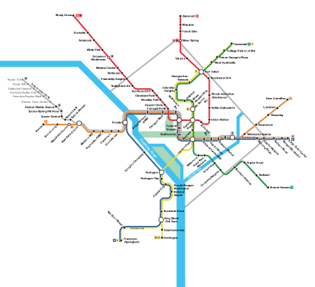
Figure 1. Map of the DC Metro network in 2012. Credit: VeggieGarden, originally posted to Wikipedia.

References

- Becker (1968) Becker, G. S. (1968): “Crime and Punishment: An Economic Approach,” Journal of Political Economy, 76, 169–217, publisher: University of Chicago Press.
- Boyd et al. (1989) Boyd, C., C. Martini, J. Rickard, and A. Russell (1989): “Fare Evasion and Non-Compliance: A Simple Model,” Journal of Transport Economics and Policy, 23, 189–197, publisher: [London School of Economics, University of Bath, London School of Economics and University of Bath, London School of Economics and Political Science].
- Chellappa and Shivendu (2005) Chellappa, R. K. and S. Shivendu (2005): “Managing Piracy: Pricing and Sampling Strategies for Digital Experience Goods in Vertically Segmented Markets,” Information Systems Research, 16, 400–417, publisher: INFORMS.
- Correa et al. (2017) Correa, J., T. Harks, V. J. C. Kreuzen, and J. Matuschke (2017): “Fare Evasion in Transit Networks,” Operations Research, 65, 165–183, publisher: INFORMS.
- Fisman and Miguel (2007) Fisman, R. and E. Miguel (2007): “Corruption, Norms, and Legal Enforcement: Evidence from Diplomatic Parking Tickets,” Journal of Political Economy, 115, 1020–1048, publisher: The University of Chicago Press.
- Jain et al. (2013) Jain, M., V. Conitzer, and M. Tambe (2013): “Security scheduling for real-world networks,” in Proceedings of the 2013 international conference on Autonomous agents and multi-agent systems, Richland, SC: International Foundation for Autonomous Agents and Multiagent Systems, AAMAS ’13, 215–222.
- Kooreman (1993) Kooreman, P. (1993): “Fare Evasion as a Result of Expected Utility Maximisation: Some Empirical Support,” Journal of Transport Economics and Policy, 27, 69–74, publisher: [London School of Economics, University of Bath, London School of Economics and University of Bath, London School of Economics and Political Science].
- Malik (1990) Malik, A. S. (1990): “Avoidance, Screening and Optimum Enforcement,” The RAND Journal of Economics, 21, 341–353, publisher: [RAND Corporation, Wiley].
- Perlman and Ozinci (2014) Perlman, Y. and Y. Ozinci (2014): “Reducing shoplifting by investment in security,” The Journal of the Operational Research Society, 65, 685–693, publisher: [Operational Research Society, Palgrave Macmillan Journals].
- Polinsky and Shavell (1979) Polinsky, A. M. and S. Shavell (1979): “The Optimal Tradeoff between the Probability and Magnitude of Fines,” The American Economic Review, 69, 880–891, publisher: American Economic Association.
- Polinsky and Shavell (1984) ——— (1984): “The optimal use of fines and imprisonment,” Journal of Public Economics, 24, 89–99.
- Polinsky and Shavell (2000) ——— (2000): “The Economic Theory of Public Enforcement of Law,” Journal of Economic Literature, 38, 45–76.
- Schmeidler (1973) Schmeidler, D. (1973): “Equilibrium points of nonatomic games,” Journal of statistical Physics, 7, 295–300.
- Slemrod (2007) Slemrod, J. (2007): “Cheating Ourselves: The Economics of Tax Evasion,” Journal of Economic Perspectives, 21, 25–48.
- Tirachini and Hensher (2012) Tirachini, A. and D. A. Hensher (2012): “Multimodal Transport Pricing: First Best, Second Best and Extensions to Non-motorized Transport,” Transport Reviews, 32, 181–202, publisher: Routledge _eprint: https://doi.org/10.1080/01441647.2011.635318.
- Yaniv (2009) Yaniv, G. (2009): “Shoplifting, monitoring and price determination,” Journal of Behavioral and Experimental Economics (formerly The Journal of Socio-Economics), 38, 608–610, publisher: Elsevier.
- Yin et al. (2012) Yin, Z., A. X. Jiang, M. Tambe, C. Kiekintveld, K. Leyton-Brown, T. Sandholm, and J. P. Sullivan (2012): “TRUSTS: Scheduling Randomized Patrols for Fare Inspection in Transit Systems Using Game Theory,” AI Magazine, 33, 59–59, number: 4.