Ab initio multi-scale modeling of ferroelectrics: The case of PbTi$\text{O}_{3}$

Abstract

We report an ab initio multi-scale study of lead titanate using the Deep Potential (DP) models, a family of machine learning-based atomistic models, trained on first-principles density functional theory data, to represent potential and polarization surfaces. Our approach includes anharmonic effects beyond the limitations of reduced models and of the linear approximation for the polarization. The calculated enthalpy, spontaneous polarization, specific heat and dielectric susceptibility agree well with experiments on single crystals. In addition, we study how the free energy depends on the polarization with enhanced sampling methods, further supporting the first-order and order-disorder character of the transition. The latter is evidenced by persistence of local dipoles above the transition temperature. The simulated free energy surface as a function of the global polarization leads to a Landau-Devonshire theory of the single domain crystal.

I Introduction

The iconic feature of ferroelectric crystals is switchable spontaneous polarization. The polarization $\mathcal{P}$ is the sum of ionic ($\mathcal{P}_{ion}$) and electronic ($\mathcal{P}_{el}$) contributions. Here, we take the ions to include nuclei and (frozen) core electrons, so that the electronic contribution is associated to the valence electrons. While $\mathcal{P}_{ion}$ is simply the sum of the dipole moments of the ions, $\mathcal{P}_{el}$ is associated, according to the modern microscopic theory  Resta and Vanderbilt (2007), to the Berry phase of the electronic state. Interestingly, this contribution can also be expressed as a sum of dipole moments Resta and Vanderbilt (2007). These are the dipole moments of the centers of the maximally localized Wannier functions that derive from a unitary transformation of the valence orbital space Marzari et al. (2012). Thus, the polarization $\mathcal{P}$ of a crystal is the sum of the dipole moments of the ions and of the Wannier centers. This sum is defined modulo a quantum associated to the periodicity of the crystalline lattice. A convenient theoretical framework to deal with the electronic degrees of freedom in the context of the adiabatic separation of electron and ion dynamics is provided by Kohn-Sham (KS) density functional theory (DFT). In this approach, that works well for (electronically) weakly-correlated ferroelectric materials, $\mathcal{P}_{el}$ is given by a sum over the occupied bands of an effective non-interacting system.

So far, using KS-DFT and suitable approximations for the exchange-correlation functional, the unique properties of ferroelectric materials have been modeled at zero temperature Zhang et al. (2017), while finite temperature modeling remains a great challenge. To circumvent the formidable computational costs of modeling finite temperature properties of ferroelectric materials within ab-initio electronic structure theory, the effective Hamiltonian approach Zhong et al. (1994, 1995) was developed, a reduced model that retains only the most important degrees of freedom. It can be viewed as a perturbative theory in the low temperature limit. In the effective Hamiltonian scheme, the adiabatic potential energy surface, i.e., the potential energy of interaction among the atoms, is approximated by the potential energy of a reduced set of collective coordinates, associated to long-wavelength phonon modes limited to the acoustic modes and the lowest frequency transverse optical (TO) modes. Anharmonicity is only included to low order in the local displacements of the soft TO modes. At the same time, the dependence of $\mathcal{P}_{el}$ on the atomic configuration is approximated linearly in terms of the Born charges associated to the soft TO modes. The model parameters are fitted to zero temperature DFT calculations. Due to its low computational cost, the effective Hamiltonian approach has been widely applied to crystalline ferroelectric materials, leading to major progress as the model could reproduce successfully, without empirical parameters, the qualitative properties of displacive-type ferroelectric perovskites Zhong et al. (1994, 1995); Waghmare and Rabe (1997); Nishimatsu et al. (2008). Notably, the predictive power of the scheme was found to deteriorate for transitions occurring at relatively high temperature where many-phonon excitations are important Tinte et al. (2003). A full account of anharmonicity would be possible with ab-initio molecular dynamics (AIMD) simulations, whereby DFT calculations are performed on the fly at each atomic configuration along atomic trajectories at finite temperature. This scheme, however, has a substantial computational cost that severely limits simulation studies of the ferroelectric transition Srinivasan et al. (2003).

Ferroelectric behavior has also been simulated with empirical force fields. In these approaches all the atomic degrees of freedom are taken into account. The empirical force fields are fitted to a limited set of DFT data, but often fail to describe the ab-initio potential energy surface with uniform accuracy, even after fine tuning  Tinte et al. (1999); Goddard et al. (2002); Grinberg et al. (2002); Brown (2009); Liu et al. (2013). These schemes, sometimes dubbed “second principles” in the literature, have been examined in a recent review article Ghosez and Junquera (2022). Problems with this methodology originate from the limited representative power of hand-crafted empirical potentials, and from the difficulty of inferring the dpendence of the electronic degrees of freedom on the atomic configurations.

In the recent years, general non-perturbative approaches have emerged in the context of statistical learning. These methods use either deep neural networks (DNN)  Zhang et al. (2018a) or Gaussian regression  Behler and Parrinello (2007) to represent uniformly and with high quantitative accuracy the potential energy surface predicted by first-principles quantum mechanical schemes, such as DFT. Related models have also been introduced to describe the dependence of the Wannier centers on the atomic coordinates Zhang et al. (2020a). These models provide a DNN representation for the polarization surface, which gives the polarization $\mathcal{P}$ as a function of the atomic configurations. The success of statistical learning methodologies for molecular simulation is enabled by several findings. First, the adiabatic potential energy and polarization surfaces can be approximated by extensive short-range models that scale with size like empirical force fields. Second, machine learning (ML) techniques can be used to optimize the models upon training on first-principles data collected on relatively small systems. Third, the optimized models typically reproduce ab initio results with chemical accuracy, i.e., with errors smaller than 1 kcal/mol. These findings are supported by studies covering a wide range of material systems and thermodynamic conditions Wu et al. (2021a); Zhang et al. (2021); Tang et al. (2020); Yang et al. (2021). Molecular dynamics (MD) with ML potentials retain the accuracy of AIMD at a much lower computational cost. For example, an efficient GPU implementation of Deep Potential (DP) molecular dynamics, a scheme based on a DNN representation, makes possible multimillion atom simulations over time scales of tens to hundreds of nanoseconds on world class supercomputers  Lu et al. (2021a).

Machine learning-assisted MD open opportunities for multiscale modelling of ferroelectric materials that one could hardly imagine in the past Dawber et al. (2005). In this context, a multiscale modelling strategy should involve the following steps. First, one should demonstrate that finite temperature simulations of AIMD quality are possible for ML models of ferroelectric materials. This was shown in recent studies of $\text{HfO}_{2}$ Wu et al. (2021a) and of monolayer $\alpha$-$\text{In}_{2}\text{Se}_{3}$ Wu et al. (2021b), using DP models trained on DFT data within the generalized gradient approximation (GGA). Next, one should focus on the ferroelectric phase transition. This was done in a recent study that addressed the sequence of phase transitions in $\text{BaTiO}_{3}$, using an approximate expression for the polarization  Gigli et al. (2021). Finally, one should perform a detailed analysis of the free energy landscape in the vicinity of the transition, which would be the starting point for constructing coarse grained mesoscopic models fully consistent with the underlying atomistic description. We emphasize the importance of achieving consistency among different scales as this has been an elusive goal of most multiscale models so far.

In this paper, we report a study targeting all the objectives listed above for the prototypical ferroelectric material lead titanate ( PbTi$\text{O}_{3}$ ). We use DP models for the potential and the polarization surfaces. The latter is described without approximation in terms of the dipole moments of the Wannier centers. With this approach, we predict accurately, from first principles electronic structure theory, the change of thermodynamic and dielectric properties across the ferroelectric phase transition. Our results include evidence for the first order character of the transition and agree well with experimental observations. Next, we use enhanced sampling techniques to compute the free energy as a function, respectively, of the magnitude of the cell dipole and of the polarization vector. From the free energy profile depending on the cell dipole amplitude we extract with unprecedented accuracy the transition point of the model. We also provide evidence that the transition is mainly driven by order-disorder effects. Finally, we analyze the free energy as a function of the polarization vector in a finite temperature range about the phase transition, finding that it can be reproduced accurately by a phenomenological Landau-Devonshire model with suitably fitted parameters. This result is a first step in the direction of establishing an effective approach for simulating mesoscopic processes in ferroelectric materials, e.g., ferroelectric domain dynamics, with a model fully derived from the microscopic Hamiltonian.

The paper is organized as follows. In section  II we report our calculated $T=0$K bulk properties of PbTi$\text{O}_{3}$ at a meta-GGA level of DFT. These results are not new but are presented for completeness. Then, we show how the information necessary to fully describe a ferroelectric material within DFT and the microscopic theory of polarization can be distilled into an ML framework. We achieve this goal by constructing two DP models, one for the adiabatic potential energy surface, the other for the dependence of the Wannier centers  Resta and Vanderbilt (2007) on the atomic environment. These two models enable deep potential molecular dynamics (DPMD) simulations that retain the accuracy of AIMD at a much lower computational cost. In section  III we use DPMD to study a single domain PbTi$\text{O}_{3}$ crystal in the $1\sim 10$nm spatial scale. The calculated enthalpy, spontaneous polarization, specific heat and dielectric susceptibility, agree well with recent experiments. In section IV we use well-tempered metadynamics  Barducci et al. (2008), a well established technique for enhanced statistical sampling, to extract from the atomistic simulations the free energy surface (FES) as a function of two collective variables (CV) associated to the polarization $\mathcal{P}$. One CV is the magnitude of the cell dipole $|\mathcal{P}|\Omega$, where $\Omega$ is the average volume of the unit cell. The corresponding FES is one dimensional (1D). The other CV is the polarization vector $\mathcal{P}$, and the corresponding FES is three dimensional (3D). The FES associated to $|\mathcal{P}|\Omega$ is used to accurately determine the character and the temperature $T_{c}$ of the phase transition, after eliminating finite size effects. The FES associated to $\mathcal{P}$ is interpolated in a finite temperature range with Landau-Devonshire-type polynomials. These results are relevant to studying single domain PbTi$\text{O}_{3}$ crystals at the $10\sim 100$nm spatial scale. Three appendices report, respectively, the details of the DFT calculations (Appendix A), the details of the training and validation of the DP models (Appendix B), and the details of the DPMD simulations (Appendix C).

II Deep Potential Model for PbTi$\text{O}_{3}$

II.1 Electronic and atomic structure from DFT

The prototypical ferroelectric perovskite crystal PbTi$\text{O}_{3}$ is the end member of the industrially important lead zirconate titanate series. It exhibits a high transition temperature, $T_{c}=763K$, and strong anharmonic effects. To model PbTi$\text{O}_{3}$ , we adopt the strongly constrained and appropriately normed (SCAN) meta-GGA functional approximation introduced in Ref. Sun et al. (2015). According to Ref. Zhang et al. (2017), SCAN systematically improves the prediction of structural and electric properties of a wide class of ferroelectric materials compared to other general purpose functional approximations, and, in some cases, it is as accurate or even more accurate than the hybrid functional B1-WC  Zhang et al. (2017), which was specifically designed for ferroectric materials.

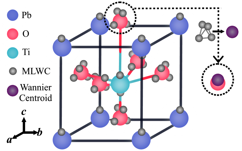
Figure 1: Conventional tetragonal cell for the ground state P4mm structure of PbTi$\text{O}_{3}$ . Atoms and valence MLWCs are indicated by spheres. Semicore MLWCs for Ti and Pb are not shown. The MLWCs can be uniquely attributed to each atom based on their distance from it. The Wannier centroid is the spatial average of the MLWCs associated to one atom, as illustrated for the topmost oxygen atom.

Detailed studies of the ground-state properties of PbTi$\text{O}_{3}$ based on the SCAN functional have been reported in the literature  Paul et al. (2017); Zhang et al. (2017), using electronic structure calculations with the projector augmented wave (PAW) method  Blöchl (1994). Here, we use plane waves and norm-conserving pseudopotentials (NCPP) Hamann et al. (1979) instead. Our results for the static properties at zero temperature are reported in Appendix A: they agree well with prior work, but for minor differences to be expected from the distinct numerical methods and convergence criteria adopted. In Fig. 1 we display a schematic representation of the ground-state P4mm tetragonal structure of PbTi$\text{O}_{3}$ , including the location of the centers of the maximally localized Wannier functions (MLWCs) Marzari et al. (2012). We further define the Wannier centroid Zhang et al. (2022) associated to an atom as the average position of the MLWCs closer to that atom.

The $c/a$ ratio in the tetragonal structure is an important geometric property that quantifies the magnitude of the ferroelectric distortion. Most functional approximations, including SCAN, overestimate the $c/a$ ratio, i.e., they suffer of the so-called supertetragonality problem. In our calculation, the optimized tetragonality of the P4mm structure is $c/a=1.142$, about 7 percent larger than the zero-temperature value of $1.071$ extrapolated from experiments Mabud and Glazer (1979). This is not a minor quantitative issue because a strong correlation exists between the magnitude of the tetragonality and the ferroelectric transition temperature. The tetragonality error indicates that available functional approximations are not sufficiently accurate to capture the fine balance between the two inequivalent Ti-O bonds along the direction of the spontaneous polarization. In the next section, we will show that, to large extent, the supertetragonality error can be corrected by applying an ad hoc hydrostatic pressure to the system, as suggested in Ref. Zhong et al. (1994). This empirical correction to the energy functional is small, of the order of 1kcal/mol, the value conventionally set to quantify chemical accuracy. Yet, it is sufficient to bring the calculated transition temperature and thermodynamic properties of PbTi$\text{O}_{3}$ in rather close agreement with experiment. With this minor empirical adjustment our multi-scale model gives invaluable insight on the physics of the ferroelectric phase transition in PbTi$\text{O}_{3}$ .

II.2 Machine Learning from DFT calculations

The electronic features needed to study the ferroelectric phase transition, are the adiabatic potential energy surface and the MLWCs that provide the natural local decomposition of $\mathcal{P}_{el}$.

We base our work on the Deep Potential (DP) methodology developed in Refs. Zhang et al. (2018a, b, 2020a). We use machine learning to construct DP models for the desired electronic structure features. One DP model, hereafter called the energy model, reproduces faithfully the Born-Oppenheimer potential energy surface of the atoms. Another DP model, hereafter called the dipole model, reproduces faithfully how $p^{G}$, the total dipole moment of the simulation cell, depends on the atomic configurations. The corresponding polarization is given by $\mathcal{P}=p^{G}/V$, where $V$ is the supercell volume. The centrosymmetric structure is taken as the reference for the zero of polarization, to fix the gauge freedom. In all our simulations, the variation of the polarization relative to the reference is small compared to the polarization quantum so that the dipole model is single-valued without ambiguity.

Upon training on sufficient DFT data, the above two models can predict with high accuracy the potential energy and the polarization of configurations independent from those used for training. Typical errors of 1 meV/atom and of $1\mu\text{C/cm}^{2}$, are found for the energy and the polarization, respectively. Importantly, the error distributions closely resemble Gaussian distributions, suggesting that the errors affecting the DP models are statistical rather than systematic. The details of the training procedure, including the training dataset are reported in Appendix B.

III Finite temperature properties from deep potential molecular dynamics

DPMD allows us to carry out large scale finite temperature simulations of bulk PbTi$\text{O}_{3}$ of ab initio MD quality. Here, we consider spatial scales of $1\sim 10$nm and observation times of $\sim 1$ns, focusing on the thermal properties of defect-free single-domain bulk PbTi$\text{O}_{3}$ .

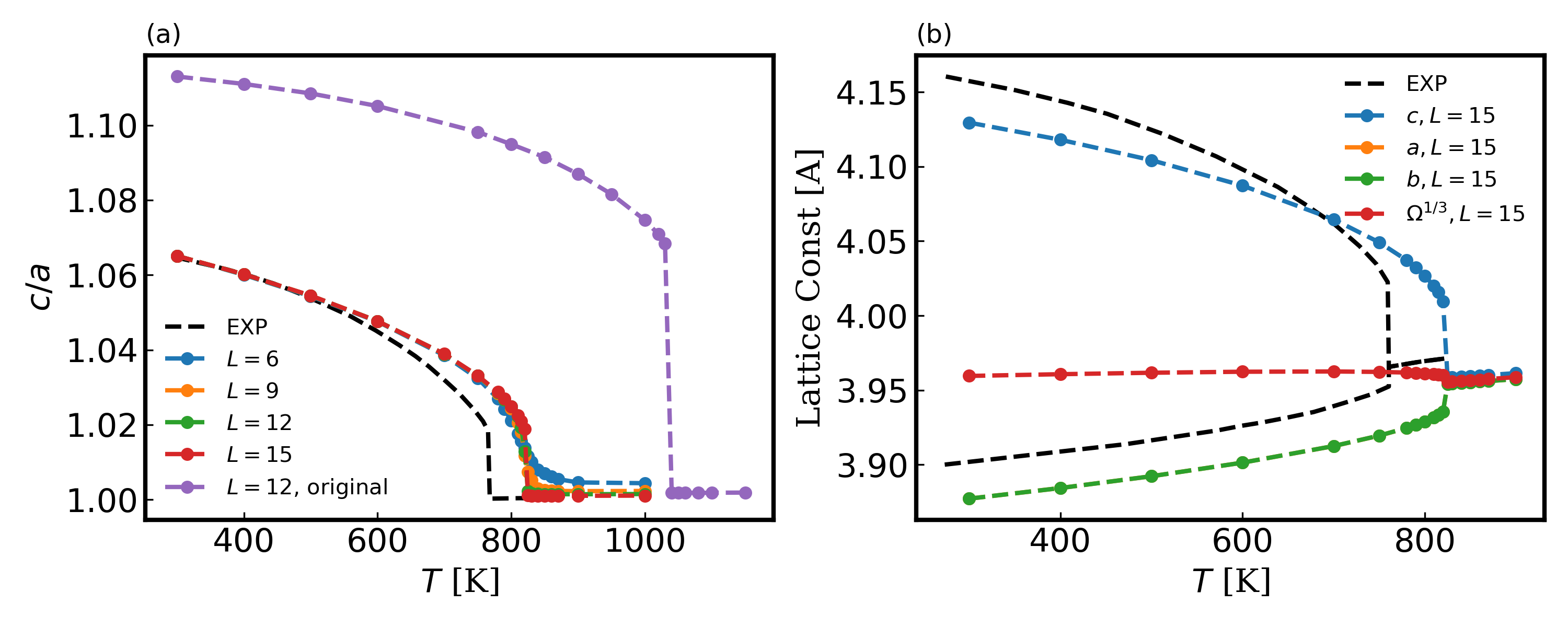
Figure 2: (a) The tetragonality of bulk PbTi$\text{O}_{3}$ for NPT-ensemble with $P=P_{0}$ (red) and $P=P_{a}+P_{0}$ (others). The experimental data are excerpted from  Mabud and Glazer (1979).(b) The lattice constants of bulk PbTi$\text{O}_{3}$ for NPT-ensemble with $P=P_{a}+P_{0}$. The orange line is overlapping with the green line thus invisible. The red line represents $\Omega^{1/3}=(abc)^{1/3}$.

An issue that needs to be addressed is the supertetragonality error of the SCAN functional approximation. The extent of this error is evident in panel (a) of Fig. 2, in which the $c/a$ ratio measured in experiments in a temperature range extending from room temperature up to $T_{c}$ and beyond, is compared with the corresponding results from DPMD simulations at ambient pressure ($P_{0}$). The large tetragonality of the theoretical model correlates with an overestimation by almost $300K$ of the transition temperature $T_{c}$ to the cubic phase. As suggested in Ref. Zhong et al. (1994), the tetragonality error can be corrected to large extent by adding an artificial hydrostatic pressure $P_{a}$ to the pressure $P_{0}$ acting on the theoretical sample. Here, we fix $P_{a}$ by requiring that the theoretical tetragonality matches experiment at room temperature ($T=300K$). A value of $P_{a}=2.8\times 10^{4}$ bar is obtained in this way. The corresponding $c/a$ ratio at different temperatures is shown in the same panel of Fig. 2 for different supercell sizes, indicated by $L\times L\times L$ in units of the elementary cell. Clearly, the additional pressure brings the tetragonality and also the transition temperature of the model in much closer agreement with experiment. The plots for different cell sizes in Fig. 2 (a) illustrate the finite size dependence of the transition, which becomes sharper with increasing size, a behavior consistent with a first-order character of the transition. The transition appears sufficiently sharp only for $L\geq 9$. Under $P=P_{a}+P_{0}$, also the lattice constants shown in Fig. 2(b) agree well with experiment over the entire temperature range. In addition, the plot shows that the DPMD simulation captures well also the small thermal expansion of the unit cell volume $\Omega=V/L^{3}$ in the cubic phase. In the following, unless otherwise specified, all the reported DPMD simulations are carried out in the NPT-ensemble with $P=P_{a}+P_{0}$.

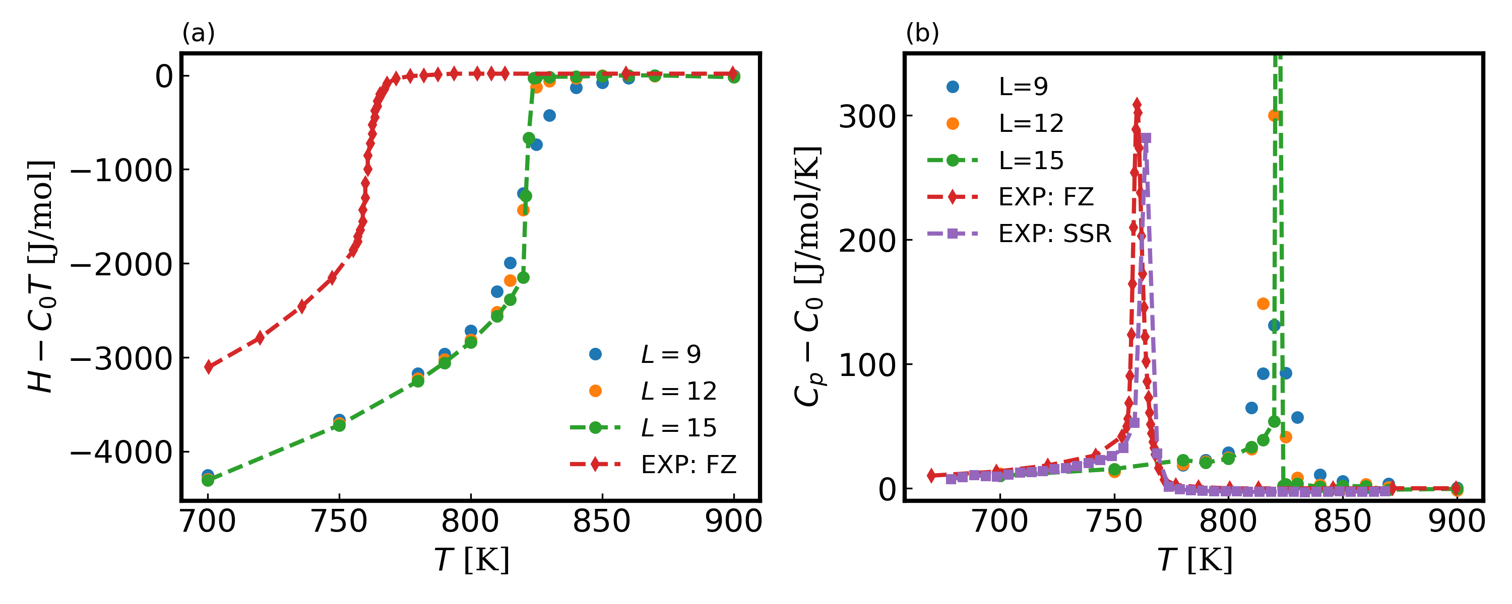
Figure 3: (a) The difference per mole between the enthalpy $H$ and $C_{0}T=3nRT$. $n=5$ is the number of atoms in one unit of PbTi$\text{O}_{3}$ . The curves are shifted along the vertical axis for easier comparison. (b) The difference between the computed specific heat $C_{p}$ and the Dulong-Petit specific heat $C_{0}=3nR$ for bulk PbTi$\text{O}_{3}$ . The experimental data are excerpted from  Rossetti and Maffei (2005) (red) and  Yoshida et al. (2009) (purple).

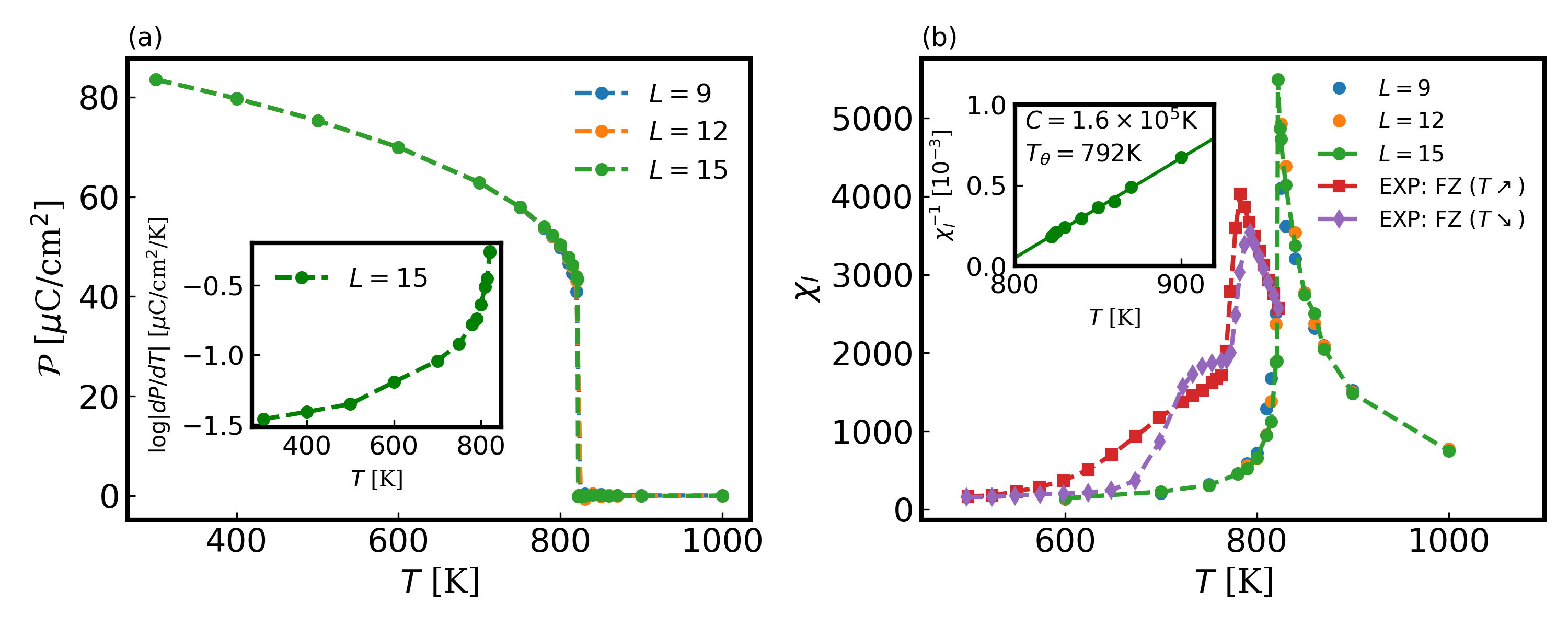
Figure 4: (a) The temperature dependence of the spontaneous polarization for finite size systems $L=9,12,15$. The inset shows the computed pyroelectric coefficient for the ferroelectric region. (b) The longitudinal susceptibility $\chi_{l}$ near transition. The experimental data taken from the heating and cooling cycles are excerpted from  Maffei and Rossetti (2004). The inset shows the Curie - Weiss behavior of $\chi_{l}^{-1}$ at the cubic phase. The guiding line is fitted to the data points (solid circle) for $L=15$.

Next, we consider the thermodynamic properties of bulk PbTi$\text{O}_{3}$ in the vicinity of the ferroelectric phase transition. Fig. 3 (a) shows the temperature dependence of the enthalpy measured in experiments and in simulations with three different cell sizes, relative to the prediction of the Dulong Petit law. In the simulations, the enthalpy $H$ is computed from the NPT-ensemble average of $E+P_{0}V$, where $E$ is the total internal energy of the system. The experimental data were measured by differential scanning calorimetry on bulk single crystals grown by the float-zone technique  Rossetti and Maffei (2005). In simulations, finite size effects are weak when $L\geqslant 12$, yielding a latent heat of about $2000$J/mol. Both in experiment and in simulations the cubic phase satisfies well the equipartition law. The experimental latent heat given by the jump of the enthalpy relative to the Dulong-Petit law at the phase transition can be roughly estimated from Fig. 3 (a). It is only slightly smaller than the DPMD prediction. In Fig. 3 (b), the specific heat $C_{p}$ obtained from the simulations is compared to the results of measurements on float-zone (FZ) samples  Rossetti and Maffei (2005), and on powder samples prepared by solid-state reaction (SSR) methods  Yoshida et al. (2009). In the simulations, $C_{p}$ is extracted from the fluctuation of $H=E+P_{0}V$ under isothermal-isobaric conditions at pressure $P$. The two experimental curves are slightly different due to different preparation methods. The bulk properties of float-zone samples should be closer to the properties of a pure single domain crystal, than the properties of powder and flux-grown ceramic samples Bhide et al. (1968); Remeika and Glass (1970). Notably, the measured specific heat of flux-grown ceramic PbTi$\text{O}_{3}$ did not show Dulong-Petit-like behavior in the cubic phase, while our computation and the two experiments shown here obey closely the Dulong-Petit law in the cubic phase. However, even float-zone samples near the transition should still contain a considerable amount of defects. In a small interval around the transition temperature, i.e., for $T=T_{c}\pm 5K$, the simulated $C_{p}$ is narrower and sharper than in experiments. The experimental observations may be affected by strain inhomogeneities Rossetti and Maffei (2005) that changed the local transition temperature in the samples, resulting in an extended phase coexistence that smoothed out the singularity of the heat capacity.

Finally, we consider finite temperature dielectric properties. With our model for the Wannier centroids, these properties can be calculated rigorously, fully including the effects of anharmonicity, in contrast to the static Born charge approximation. The results are shown in Fig. 4. Panel (a) displays the temperature dependence of the spontaneous polarization $\mathcal{P}$. The computed $\mathcal{P}$ at $T=300$K is equal to $84\mu\text{C}/\text{cm}^{2}$. The computed pyroelectric coefficient ($d\mathcal{P}/{dT}$) at the same temperature is $34\text{nC}\cdot\text{cm}^{-2}K^{-1}$. So far, relatively accurate measurements of bulk $\mathcal{P}$ are obtained from extrapolation of thin films results. The $\mathcal{P}$ values at room temperature, estimated in this way, vary from $70\mu\text{C}/\text{cm}^{2}$ to $100\mu\text{C}/\text{cm}^{2}$ Nishino et al. (2020); Dahl et al. (2009); Morita and Cho (2004). The room temperature values for the pyroelectric coefficient estimated in experiments are in the range from $24\text{nC}\cdot\text{cm}^{-2}K^{-1}$ to $27\text{nC}\cdot\text{cm}^{-2}K^{-1}$ Deb et al. (1995); Iijima et al. (1986). Our simulation results are compatible with these experimental values. Fig. 4 (b) shows $\chi_{l}(T)$, the longitudinal zero-field static dielectric susceptibility of bulk PbTi$\text{O}_{3}$ . In the simulations, well-converged $\chi_{l}(T)$ for different cell sizes are computed from the fluctuation of the polarization. $\chi_{l}(T)$ has a sharp peak near $T=821$K, providing additional evidence for a first order ferroelectric transition in pure single-domain PbTi$\text{O}_{3}$ . For comparison, the float-zone experimental data  Maffei and Rossetti (2004), reported in the same figure, show a shoulder at $T=763K$, the experimental phase transition temperature, and a broader peak shifted to temperatures closer to $T=793$K. This obvious distortion may come from domain pinning caused by internal stresses in the sample Maffei and Rossetti (2004). Notably, the computed $\chi_{l}(T)$ is quantitatively closer to recent measurements on float-zone samples Maffei and Rossetti (2004) than to the measurements on ceramic samples Remeika and Glass (1970); Bhide et al. (1962). The good agreement of our results with experiments is a consequence of the fact that our dipole model captures accurately the behavior of the electronic degrees of freedom responsible for the dielectric response. Moreover, our simulations use space and time scales sufficiently large for good statistical convergence.

The computed susceptibility allows examination of the Curie - Weiss law for PbTi$\text{O}_{3}$ . The inset of Fig. 4 (b) shows a very good linear temperature dependence of $\chi_{l}(T)^{-1}$ in the cubic phase. The optimized Curie constant is $C=1.6\times 10^{5}$K. The extrapolated Curie temperature is $T_{\theta}=792$K. The temperature gap $\delta T=T_{c}-T_{\theta}$ is of $29$K, when using the value of $T_{c}=821$K extracted from the free energy studies discussed in the next section. The simplest Landau theory for a first order transition stipulates that the polarization dependent free energy satisfies $F(T,\mathcal{P})=A_{0}(T-T_{\theta})\mathcal{P}^{2}-B_{0}\mathcal{P}^{4}+C_{0}\mathcal{P}^{6}$. From this expression one estimates a lower bound for phase coexistence given by $T_{\theta}$ and an upper bound given by $T^{*}=T_{c}+\delta T/3$. Hence a rough estimation of $T^{*}$ is $831$K. The experimental estimation of $C$ and $T_{\theta}$ usually relies on fitting a few susceptibility or heat capacity data in a temperature region above the phase transition. Previously reported $C$ values vary from $1.1\times 10^{5}$K to $4.1\times 10^{5}$K Bhide et al. (1968); Rossetti and Maffei (2005); Remeika and Glass (1970). The large uncertainty in the experimental estimate of $C$ likely reflects a large concentration of defects in the experimental samples. Our calculation suggests that for pure single domain PbTi$\text{O}_{3}$ , $C$ should be closer to the lower end of the experimental range.

IV Free energy surfaces from atomistic modeling

In this section, we present a coarse-grained description of the ferroelectric transition. In general, coarse grained descriptions are obtained by mapping the Boltzmann weight of an atomic system with generalized coordinates $\{\alpha_{i}\}$ and Hamiltonian $\mathcal{H}(\{\alpha_{i}\})$ onto a set of collective variables (CVs) $\{\zeta_{j}\}$ through non-invertible functions $\{f_{j}\}$. The resulting equilibrium free energy surface $G(T,\{\zeta_{j}\})$ is given by

$$e^{-\beta G(T,\{\zeta_{j}\})}\propto\int\prod_{i}d\alpha_{i}e^{-\beta\mathcal{H}(\{\alpha_{i}\})}\prod_{j}\delta(\zeta_{j}-f_{j}(\{\alpha_{i}\})).$$ (1)

In ferroelectric materials, which are characterized by a spontaneous onset of non-zero polarization, the polarization is the natural CV. We use the polarization in two ways to describe the ferroelectric behavior near the phase transition.

In the first approach, we calculate the 1-D free energy surface $G(T,|p^{G}|)$ as a function of the magnitude of the average unit cell dipole $|\mathcal{P}|\Omega$, given by

$$G(T,|p^{G}|)=-\frac{1}{\beta}\ln\int d\mathbb{R}e^{-\beta\mathcal{H}(\mathbb{R})}\delta(|\mathcal{P}(\mathbb{R})|\Omega(\mathbb{R})-\frac{|p^{G}|}{N}).$$ (2)

Here the polarization $\mathcal{P}$ and the average unit cell volume $\Omega=V/N$ are written explicitly as functions of the generalized coordinates $\mathbb{R}$. The supercell size $N$ equals $L^{3}$ for all the $L\times L\times L$ supercells used in our simulation. $G(T,|p^{G}|)$ is calculated accurately with well-tempered metadynamics Barducci et al. (2008). The results are reported in Sec. IV.1.

The second approach focuses on the full 3-D free energy surface $\mathcal{G}(T,\mathcal{P})$ as a function of the global polarization vector $\mathcal{P}$, given by

$$\mathcal{G}(T,\mathcal{P})=-\frac{1}{\beta}\ln\int d\mathbb{R}e^{-\beta\mathcal{H}(\mathbb{R})}\delta(\mathcal{P}(\mathbb{R})-\mathcal{P}).$$ (3)

This requires sampling a 3-D domain of the collective variable $\mathcal{P}$, which is demanding but still possible with well-tempered metadynamics, taking advantage of the symmetry of the free energy surface. Having extracted the free energy landscape $\mathcal{G}(T,\mathcal{P})$ from the simulations, we can make contact with phenomenological models, such as the Landau-Devonshire (LD) theory, that would allow modeling at the mesoscale. To date there have been many attempts to connect microscopic models based on the effective Hamiltonian approach to LD theory. Some efforts sought to match the equilibrium polarization predicted by the microscopic model with the corresponding prediction from LD theory Íñiguez et al. (2001), while other efforts sought to determine the parameters of LD theory from free energy differences calculated with thermodynamic integration from polarization-constrained MD Geneste (2009); Kumar and Waghmare (2010). Here, we compute $\mathcal{G}(T,\mathcal{P})$ directly from DPMD simulations using well-tempered metadynamics. The results are reported in Sec. IV.2.

IV.1 1-D free energy surface

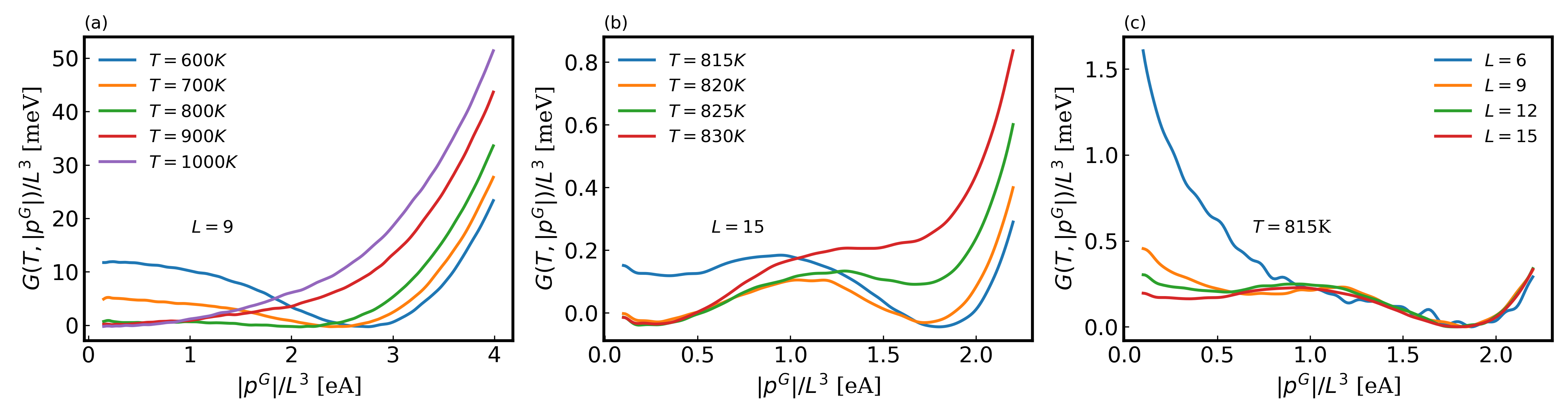
Figure 5: (a) $G(T,|p^{G}|)$ per unit of PbTi$\text{O}_{3}$ . (b) $G(T,|p^{G}|)/L^{3}$ near the transition. (c) $G(T=815K,|p^{G}|)/L^{3}$ computed for different sizes of supercell. The barrier height between two basins shown in the figure is almost constant for $L\geq 9$, suggesting that the free energy barrier scales with the volume of the supercell, pointing to the importance of entropic volume effects in promoting the phase transition (see text). The wiggles in the $L=6$ curve result mostly from insufficient self-averaging in a small supercell and can be reduced by extending the time scale of the simulations.

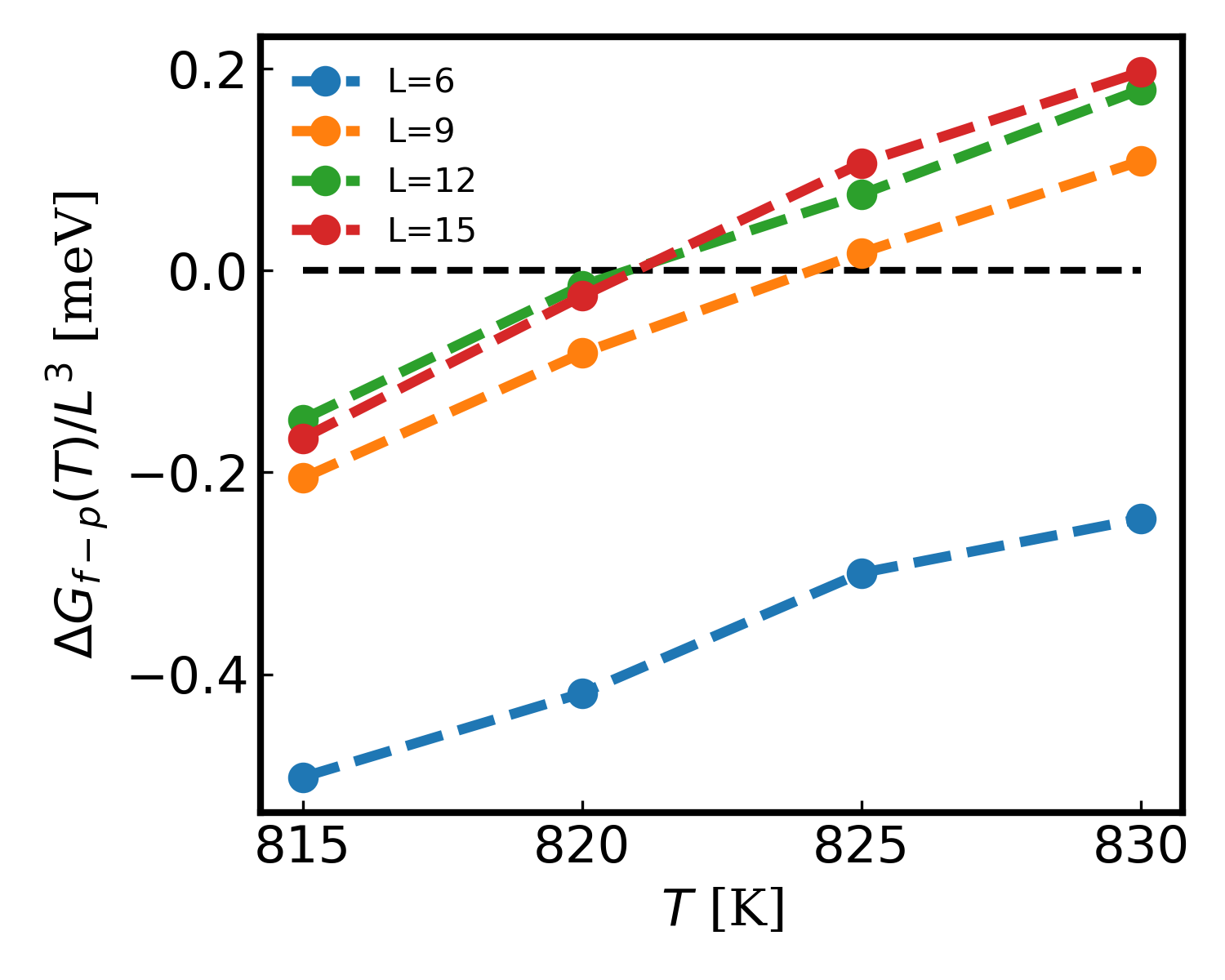
Figure 6: Free energy difference $\Delta G_{f-p}(T)$ computed with different finite sizes.

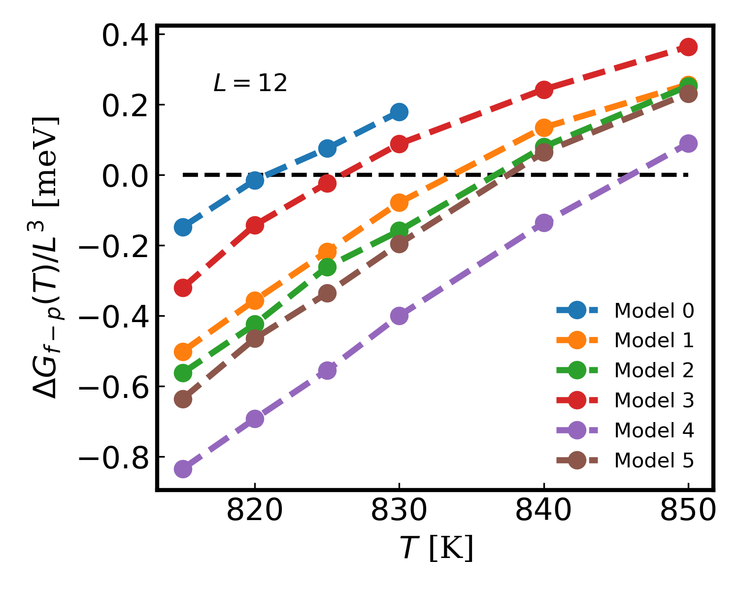
Figure 7: Free energy difference $\Delta G_{f-p}(T)$ computed with the ensemble of models at $L=12$. Model 0 indicates the original energy and dipole models.

We use the 1-D free energy surface $G(T,|p^{G}|)$ to accurately determine the order and the temperature of the phase transition. We start by looking at the free energy profile on a coarse energy scale where it is difficult to discern finite size effects. The corresponding $G(T,|p^{G}|)$ scaled by $L^{-3}$ is plotted against $|p^{G}|/L^{3}\in$[$0.15$eÅ,$4$eÅ] in Fig. 5 (a) for $T\in[600\text{K},1000\text{K}]$. The calculations use a supercell with $L=9$. From a quick inspection it appears that the phase transition occurs near $T=800K$. The free energy is plotted on a much finer energy scale near the phase transition in Fig. 5 (b). Here, we use a large supercell with $L=15$ to minimize size effects, and run $4$ns metadynamics simulations to reduce the stochastic error in $G(T,|p^{G}|)/L^{3}$ to the order of $0.01$meV. Details of convergence are presented in Appendix C. Fig. 5 (b) suggests that the upper bound for phase coexistence is around $830$K, in good agreement with our previous estimate of $T^{*}\approx 831$K from Landau theory. Experimentally, the ferroelectric phase transition in PbTi$\text{O}_{3}$ is first order. Our DP model, based on the SCAN-DFT functional, agrees with experiment on that, as the first order nature of the phase transition is predicted by both the direct atomistic simulations presented in Sec. III and by the present analysis of the free energy profile.

It is instructive to analyze how finite size affects $G(T,|p^{G}|)$. Fig. 5 (c) shows how the calculated free energy profile at $T=815$K changes by changing the size of the simulation cell from $L=6$ (side length $\approx$ 2nm) to $L=15$ (side length $\approx$ 6nm). Small cells clearly destabilize the paraelectric phase. The effect is strong enough for the metastable paraelectric phase at $T=815$K to completely disappear when $L=6$. This suggests that order-disorder effects could play a key role in the phase transition, a hypothesis that is strongly supported by the calculated distributions of the local dipole moments at the transition. We define the local dipoles to be the dipole moments of the unit cells belonging to the supercell of the simulation. For the $L=12$ supercell, paraelectric and ferroelectric phases coexist at $T=820K$. The corresponding distributions of the magnitudes of the local dipole moments are close to Gaussian distributions, with mean near $1.7e$Å in the paraelectric phase and near $2.2e$Å in the ferroelectric phase. The standard deviation is essentially the same, $0.7e$Å, in both phases. Thus, the magnitude of the local dipole does not vanish in the centrosymmetric phase when $T=T_{c}$, as one would expect for a purely displacive transition. This result indicates that the transition is driven primarily by order-disorder effects. To further support this conclusion, we note that the centrosymmetric configuration is always energetically unfavorable in PbTi$\text{O}_{3}$ . SCAN-DFT predicts that the perfect cubic cell is unstable against polar structural distortions along the [111] directions  Paul et al. (2017). This instability favors an ordered [001] soft mode transition near $T_{c}$, but the disorder effects, that are strong near $T_{c}$ due to thermal fluctuations, are sufficient to average out the local polar distortions and stabilize the cubic phase. Accurate modelling of these disorder effects requires sufficiently large supercells in order for the entropy gained by disorder to overcome the enthalpy gain of the ordered soft mode transition. Disorder explains the stark difference between the energy profiles for $L=6$ and $L=9$ in Fig. 5 (c). Additionally, order-disorder effects should account for the weak local minimum of the free energy in the paraelectric phase, seen in Fig. 5 (b-c), for small but non-zero values of $|p^{G}|/L^{3}$. As shown by the curves in Fig. 5 (c) the small non-zero value of the dipole gets closer to zero for larger $L$, suggesting that it should converge to zero in the thermodynamic limit. This delicate effect appears clearly in Fig. 5 (c), demonstrating the accuracy of our well-tempered metadynamics simulations.

These results are fully consistent with the experimental finding that the ferroelectric phase transition in PbTi$\text{O}_{3}$ is not an ideal displacive transition Nelmes et al. (1990); Ravel et al. (1993); Sicron et al. (1994); Ravel et al. (1995). A major role of order-disorder effects in driving the phase transition in PbTi$\text{O}_{3}$ was pointed out in a recent reverse Monte Carlo study using an empirical model fitted to a wealth of experimental data Datta et al. (2018). Here, we provide ab initio evidence for this effect and open the gate to direct MD modelling of stochastic instabilities in ferroelectrics taking full account of the electronic degrees of freedom.

The above discussion shows that achieving convergence with respect to size is extremely important when modelling ferroelectric phase transitions. MD simulations of sufficiently large scale, like those presented here, are possible with DP models Lu et al. (2021b) on computer clusters of moderate size.

The relative stability of ferro- and para-electric phases can be estimated from the relative depth of the local free energy minima in Fig. 5 (b). This estimate ignores thermal fluctuations of the order parameter about the local minima. A better definition of the free energy difference $\Delta G_{f-p}(T)$ between ferro- and para-electric phases including fluctuations of the order parameter is given by

$$\small\Delta G_{f-p}(T)=-\frac{1}{\beta}\ln\frac{\int d\mathbb{R}e^{-\beta\mathcal{H}(\mathbb{R})}\Theta(|\mathcal{P}(\mathbb{R})|\Omega(\mathbb{R})-\mathfrak{P})}{\int d\mathbb{R}e^{-\beta\mathcal{H}(\mathbb{R})}(1-\Theta(|\mathcal{P}(\mathbb{R})|\Omega(\mathbb{R})-\mathfrak{P}))},$$ (4)

Here, $\Theta$ is the Heaviside step function, and $\mathfrak{P}$ is a threshold parameter that distinguishes the two minima with the magnitude of the cell dipole. In our calculations, we set $\mathfrak{P}$ to be equal to $1$eÅ, a value that ensures a good identification of the two phases. For $L>9$, $\Delta G_{f-p}(T)$ is unaffected by small changes in the value $\mathfrak{P}$. Eq. (4) can be equivalently written as

$$\Delta G_{f-p}(T)=-\frac{1}{\beta}\ln\frac{\langle\Theta(|\mathcal{P}|\Omega-\mathfrak{P})\rangle}{\langle 1-\Theta(|\mathcal{P}|\Omega-\mathfrak{P})\rangle}$$ (5)

in terms of the NPT ensemble average $\langle\cdot\rangle$.

For $L=15$, the largest supercell in our simulations, the thermal fluctuation near $T_{c}$ is of the order of $k_{B}T_{c}\approx 70$meV, which is several times smaller than the free energy barrier separating para- and ferro-electric phases given by $0.1$meV$\cdot L^{3}\approx 338$meV. The crossing of this barrier is infrequent on a time scale of nanoseconds. To facilitate barrier crossing, we add a bias potential $V_{b}$ to the Hamiltonian for an efficient evaluation of $\Delta G_{f-p}(T)$. In terms of the averages calculated in the biased ensemble, the expression for $\Delta G_{f-p}(T)$ takes the form:

$$\small\Delta G_{f-p}(T)=-\frac{1}{\beta}\ln\frac{\langle\Theta(|\mathcal{P}|\Omega-\mathfrak{P})e^{\beta{V_{b}}}\rangle_{V_{b}}}{\langle(1-\Theta(|\mathcal{P}|\Omega-\mathfrak{P}))e^{\beta{V_{b}}}\rangle_{V_{b}}}.$$ (6)

Here $\langle\cdot\rangle_{V_{b}}$ indicates NPT average in presence of an additional Boltzmann factor $e^{-\beta{V_{b}}}$, where the bias potential is constructed on the fly according to the well-tempered metadynamics prescription  Barducci et al. (2008). At convergence, the bias potential is related to the free energy $G(T,|p^{G}|)$ via

$$V_{b}(\mathbb{R})=\frac{1-\gamma}{\gamma}G(T,|\mathcal{P}(\mathbb{R})|V(\mathbb{R}))$$ (7)

where $V(\mathbb{R})$ is the volume of the supercell and $\gamma>0$ is a constant bias factor. In our simulations, $\gamma/\beta$ was adjusted to scale roughly with the height of the free energy barrier separating the two phases. This ensures good sampling of the two basins and frequent barrier crossings for the large supercells.

We use Eq. (6) to compute $\Delta G_{f-p}(T)$ for $L\in[6,9,12,15]$ and $T\in[815,820,825,830]$K with $\mathfrak{P}=1\text{e}$Å. The results are plotted in Fig. 6. For $L=12$ and $L=15$, $\Delta G_{f-p}(T)$ is essentially independent of the value of $\mathfrak{P}$, when this is varied in the interval [$0.9$eÅ,$1.2$eÅ]. The same variation of $\mathfrak{P}$ changes $\Delta G_{f-p}(T)$ by approximately $0.1$meV$\cdot L^{3}$ for $L=6$ and by approximately $0.01$meV$\cdot L^{3}$ for $L=9$. Fig. 6 shows that finite size effects stabilize the ferroeletric phase and impact negligibly the phase transition temperature when $L\geqslant 12$. Linear interpolation for $L=12$ and $L=15$ gives $T_{c}=(821\pm 1)K$. By comparison, conventional effective Hamiltonian models, not including optical modes, and higher-order effective Hamiltonian models, including anharmonic coupling between the soft mode and the TO modes, based on SCAN-DFT, predict $T_{c}=630K$ and $T_{c}=675K$, respectively, without artificial pressure correction for the tetragonality error  Paul et al. (2017). Thus, the partial anharmonic correction in the effective Hamiltonian context, raises $T_{c}$ by $45K$. However, without artificial pressure to correction, our DP model, which fully includes anharmonicity, supports a transition temperature $T_{c}$ between $1000K$ and $1050K$ (see Fig. 2(a)). The significant difference found in the predicted $T_{c}$ of DP and effective Hamiltonian models derived from the same DFT functional, is a measure of the important role played by anharmonicity in the vicinity of $T_{c}$ in PbTi$\text{O}_{3}$ .

The phase transition temperature $T_{c}$ calculated above for the DP model is only an approximation of the transition temperature of SCAN-DFT. To roughly quantify the DP error we note that the standard deviation of our energy model relative to SCAN-DFT is of approximately $1$meV per atom. As shown in Appendix B, the error distributions of the DP energy and forces are close to unbiased Gaussian distributions. Thus, we may expect that the corresponding error for the characteristic energy $k_{B}T_{c}$ should be also normally distributed with a standard deviation of the same order of the energy error.

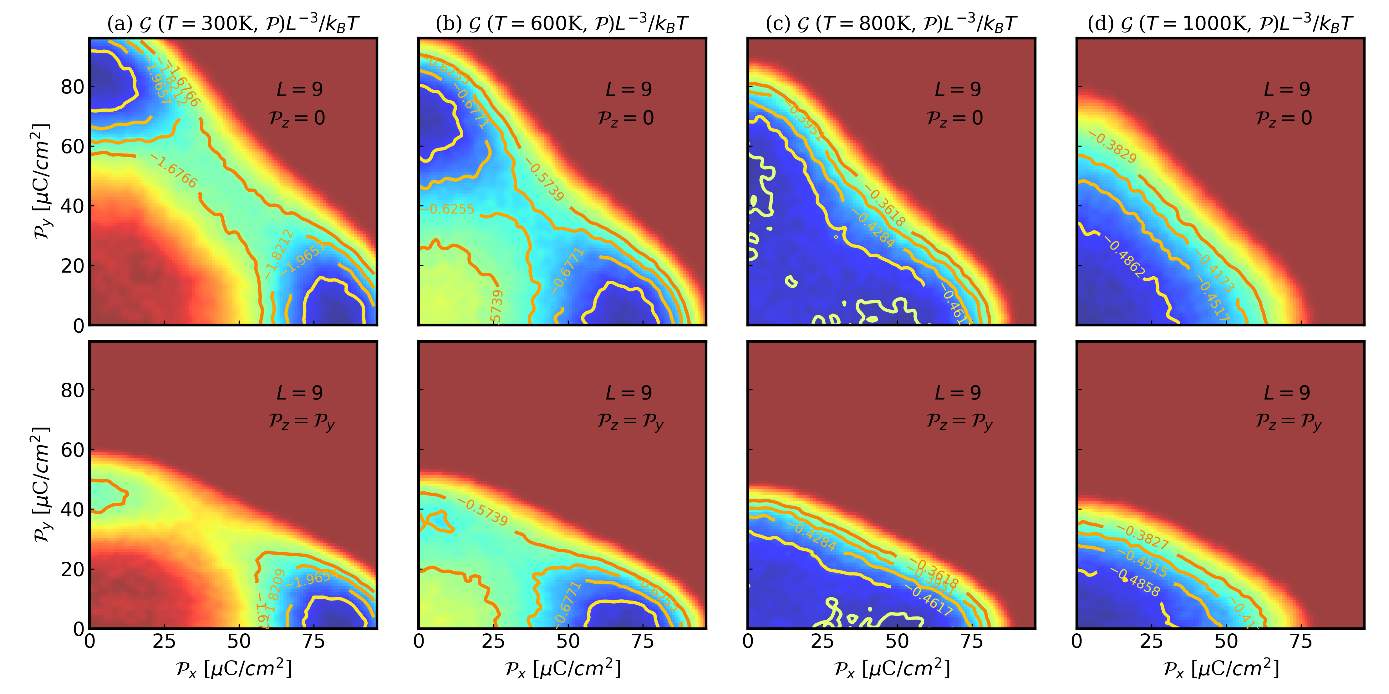
Figure 8: The colored cross-sectional representation of the free energy $\mathcal{G}(T,\mathcal{P})/L^{3}$. The unit of energy is $k_{B}T$. The red (including blended red) areas are poorly explored or unexplored.

To better estimate the uncertainty of the DP model, we trained 6 energy models and 6 dipole models with the same neural network structure and training dataset, but with different random initializations of the network parameters. All these models show Gaussian error distributions with similar standard deviations. The tetragonality of these models at $T=300$K fluctuates between $1.064$ and $1.066$ under the same artificial pressure $P_{a}=2.8\times 10^{4}$ bar applied to the original DP model to reduce the tetragonality error. The corresponding spontaneous polarization under the same NPT constraints applied to the original DP model, varies between $83\mu\text{C}/\text{cm}^{2}$ and $84\mu\text{C}/\text{cm}^{2}$. At the same time, the free energies $\Delta G_{f-p}(T)/L^{3}$ of the models near $T_{c}$ differ from each other by energies of the order of $0.1$meV, as shown in Fig. 7. The average transition point is $\overline{T_{c}}=(833\pm 8)$K. The spread of $T_{c}$ in the ensemble of DP models can be taken as an estimate of the DP error relative to SCAN-DFT. The phase transition is first order in all the models, with very similar derivatives $d\Delta G_{f-p}(T)/dT$ at the transition. Thus, even though the energy barrier separating the two phases at $T_{c}$ is of the order of $0.1$meV per unit cell (see Fig. 5), much smaller than the potential energy error of $1$meV per atom, different, but equally trained, DP models consistently predict strikingly similar phase transitions, pointing to the robustness of the model predictions. To conclude, there is no physical significance in the quantitative differences between the predictions the DP models. In the following, we will stick with the original DP model, i.e., model 0, for consistency.

IV.2 3-D free energy surface

Here, we focus on the full 3-D free energy surface as a function of the polarization vector $\mathcal{P}$. We consider single-domain bulk PbTi$\text{O}_{3}$ under no strain and in absence of externally applied electric field.

The free energy $\mathcal{G}(T,\mathcal{P})$ is invariant under mirror reflections and permutations of the Cartesian components of $\mathcal{P}$. Exploiting the symmetry, $\mathcal{G}(T,\mathcal{P})$ is calculated with well-tempered metadynamics only inside the sector $\mathcal{P}_{cut}\geqslant\mathcal{P}_{x}\geqslant\mathcal{P}_{y}\geqslant\mathcal{P}_{z}\geqslant 0$. We adopt a cutoff $\mathcal{P}_{cut}=96\mu\text{C}/\text{cm}^{2}$, use a dense 3-D grid to represent the $\mathcal{P}$ sector, and compute the free energy $\mathcal{G}(T,\mathcal{P})$ on the dense $\mathcal{P}$ grid at discrete temperature values ( $T\in[300,600,700,800,820,900,1000]$K ). Given the large number of calculations required to represent the 3-D free energy surface, we use here $L=9$ supercells to avoid excessive computational cost. With this choice, finite size effects are rather small. For instance, with $L=9$ the error on $T_{c}$, shown in Fig. 6, amounts to a few Kelvin degrees. This is insignificant on the scale of the temperature domain of interest, which spans several hundreds degrees, with a majority of temperatures far removed from $T_{c}$.

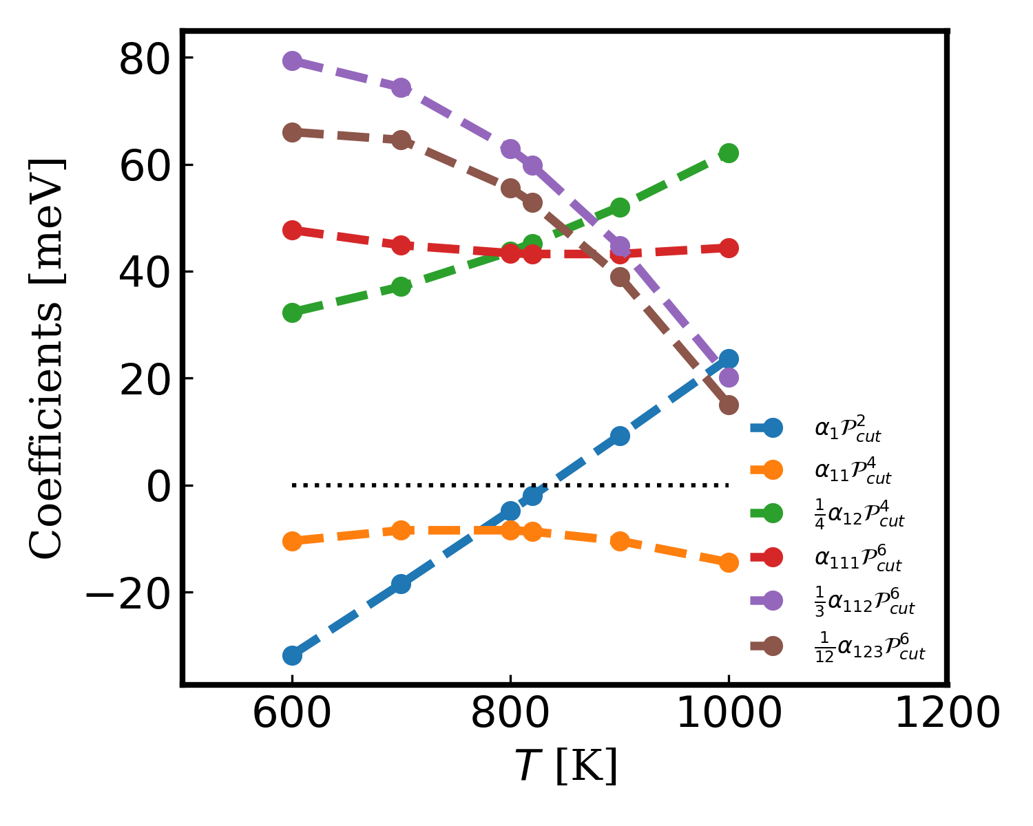
Figure 9: The regularized LD coefficients obtained through least-squared fitting in the well-explored region of $\mathcal{G}(T,\mathcal{P})$.

Cross sections of the computed $\mathcal{G}(T,\mathcal{P})$ are plotted in Fig. 8. These results are fully compatible with the 1-D profiles discussed in the previous subsection. The contour lines in Fig. 8 are noisy due to the difficulty of metadynamics simulations to converge smoothly when adopting multidimensional CVs, like the 3-D polarization vector used here. Details on the evolution of the contour lines with the simulation time are presented in Appendix C. If higher accuracy were sought, one could use enhanced variational sampling techniques, which allow multidimensional CVs and can achieve uniformly accurate sampling over a full, continuously connected, thermodynamic domain Valsson and Parrinello (2014); Invernizzi et al. (2020).

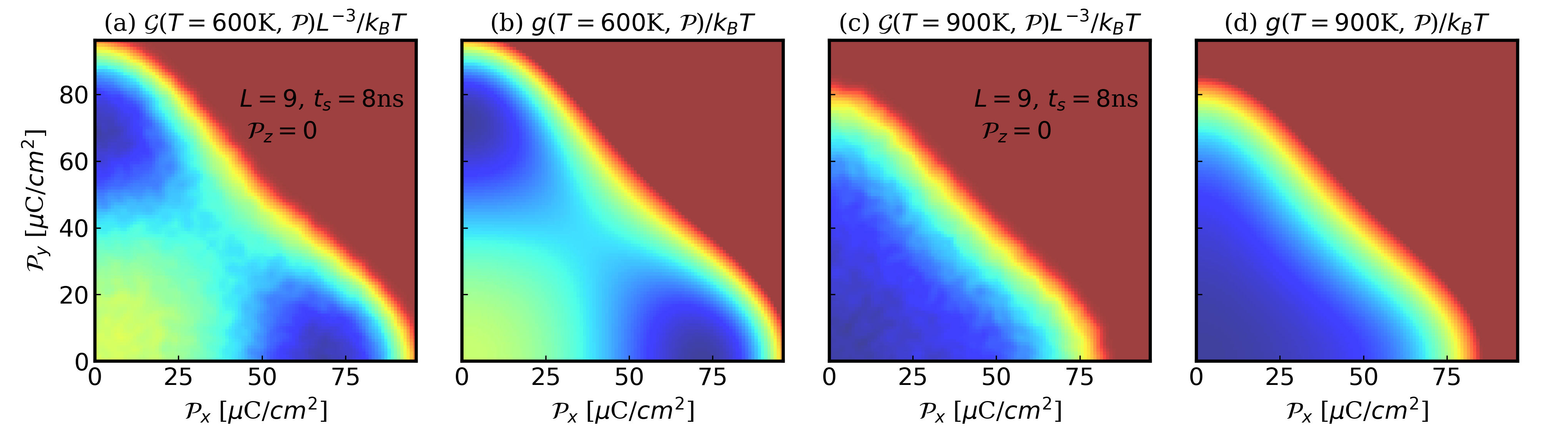
Figure 10: The colored representation of the $\mathcal{P}_{z}=0$ section of $\mathcal{G}(T,\mathcal{P})L^{-3}/k_{b}T$ compared to the optimal fitting $g(T,\mathcal{P})$ at $T=600$K and $T=900$K.

For the present purposes, however, the representation of $\mathcal{G}(T,\mathcal{P})$ achieved with well-tempered metadynamics is good enough, as it converges to a well defined 3-D surface, in spite of the statistical noise. It is instructive to compare our calculated free energy surface with the predictions of the classical Landau-Devonshire (LD) theory. The latter is based on a perturbative expansion of the free energy in powers of the polarization in the vicinity of a phase transition. Taking spatial symmetry into account, the LD free energy per PbTi$\text{O}_{3}$ unit is given by

$$\begin{split}g&=g_{0}+\alpha_{1}\|\mathcal{P}\|^{2}+\alpha_{11}(\mathcal{P}_{x}^{4}+\mathcal{P}_{y}^{4}+\mathcal{P}_{z}^{4})\\ &+\alpha_{12}(\mathcal{P}_{x}^{2}\mathcal{P}_{y}^{2}+\mathcal{P}_{x}^{2}\mathcal{P}_{z}^{2}+\mathcal{P}_{y}^{2}\mathcal{P}_{z}^{2})+\alpha_{111}(\mathcal{P}_{x}^{6}+\mathcal{P}_{y}^{6}+\mathcal{P}_{z}^{6})\\ &+\alpha_{112}[\mathcal{P}_{x}^{4}(\mathcal{P}_{y}^{2}+\mathcal{P}_{z}^{2})+\mathcal{P}_{y}^{4}(\mathcal{P}_{z}^{2}+\mathcal{P}_{x}^{2})+\mathcal{P}_{z}^{4}(\mathcal{P}_{x}^{2}+\mathcal{P}_{y}^{2})]\\ &+\alpha_{123}\mathcal{P}_{x}^{2}\mathcal{P}_{y}^{2}\mathcal{P}_{z}^{2}\end{split}$$ (8)

where $g_{0}$ is the Gibbs free energy per unit volume of the unpolarized reference system. Non-zero isotropic coefficients $\alpha_{1}$, $\alpha_{11}$, and $\alpha_{111}$ are required for a first-order transition. In particular, $\alpha_{1}$ should depend linearly on $(T-T_{\theta})$, while $\alpha_{11}$ should be less than zero and $\alpha_{111}$ should be greater than zero, in order to have a first order transition. LD theory also suggests that $T_{c}-T_{\theta}=\alpha_{11}^{2}/4\alpha_{1}\alpha_{111}$ and $T^{*}-T_{\theta}=\alpha_{11}^{2}/3\alpha_{1}\alpha_{111}$. In the classical formulation of the theory, the temperature dependence of all the coefficients is ignored, with the exception of $\alpha_{1}$. In spite of its oversimplification, the LD model gives invaluable phenomenological understanding on the ferroelectric phase transition. When applying the LD model to specific materials, some of above simplifications on the coefficients should be relaxed, as it was found that for better quantitative agreement with the properties of realistic material models, a smooth temperature dependence of all the LD coefficients should always be assumed Gonzalo and Rivera (1971); Íñiguez et al. (2001).

We found that an LD model describes accurately the free energy surface $\mathcal{G}(T,\mathcal{P})$ of the DP model in the temperature interval $[600\text{K},1000\text{K}]$, by minimizing the $l^{2}$-norm of the free energy difference between the models. In this procedure we assume that each LD coefficient has a smooth temperature dependence that is well approximated by a second order polynomial like $a_{0}+a_{1}T+a_{2}T^{2}$. The parameters $a_{0}$, $a_{1}$, and $a_{2}$ are determined by the least square fit for each LD coefficient. The resulting temperature dependence of the LD coefficients for $T\in[600\text{K},1000\text{K}]$ is displayed in Fig. 9. The fitting accuracy is quite good, as demonstrated by the small deviation of the free energy extracted from the atomistic simulations and the optimized LD free energy. Over the entire temperature interval, the free-energy deviation is found to be normally distributed about zero with standard deviation between $0.04$ and $0.06$meV/atom. This error originates mainly from the statistical error in the atomistic 3-D free energy surface, which is several times larger than that of the 1-D free energy profile $G(T,|p^{G}|)$. Fig. 10 illustrates how well $\mathcal{G}(T,\mathcal{P})/L^{3}$ is reproduced by the fitted $g(T,\mathcal{P})$ at the two temperatures $T=600$K and $T=900$K. For temperatures below $600$K, the fitting error grows larger and the deviations cease to be normally distributed, suggesting that a 6-th order LD theory may be insufficient to extrapolate the free energy surface to conditions that are too different from those at the phase transition. However, sufficiently close to the transition, in the interval $T\in[600\text{K},1000\text{K}]$, $\alpha_{1}$ shows good linear dependence on temperature, with $\alpha_{1}=0.15(T-835K)\frac{\text{meV}\cdot\text{m}^{4}}{\text{C}^{2}\text{K}}$. From the Curie-Weiss law this slope corresponds to $C\approx 1.5\times 10^{5}$K, which matches well the experimental value of $C$ reported in Ref. Haun et al. (1987). The fitted $T_{\theta}=835$K is slightly higher than the computed phase transition temperature of $T_{c}\approx 825$K for $L=9$. This overestimation may be due, in part, to the error of the least square fitting procedure, and, in part, to the limitations of the 6-th order LD expansion. Interestingly, both $\alpha_{11}$ and $\alpha_{111}$ show almost no temperature dependence, as predicted by the LD theory. The other LD coefficients show a monotonic temperature dependence.

V Conclusion

In this paper, we presented an ab initio multi-scale modeling strategy for ferroelectric materials using the case study of PbTi$\text{O}_{3}$ as an example. In our approach, multiple models with increasing degrees of coarse-graining are unified in a systematic and consistent way. From DFT to the atomistic level, the consistency is ensured by the ab initio level description of potential and polarization surfaces. From the atomistic level to the homogeneous domain level, the consistency is ensured by a direct calculation of the free energy as a function of the relevant collective variables. This allows us to obtain ab initio free energy surfaces and the corresponding effective LD theory in a continuous range of temperatures. At each transition of scale, the error caused by the distillation of a coarser grain model is quantifiable and controlled. The accumulated error is considerably smaller than the inherent error of the underlying first-principles model.

The multi-scale approach presented here can be viewed as a first step towards a more sophisticated description of multi-domain structures. The outlook is to study the mechanism of ferroelectric switching, which is shown to be non-homogeneous and dependent on the spatial scale in thin film experiments Ducharme et al. (2000); Nagarajan et al. (1999); Pertsev et al. (2003); Dawber et al. (2005). The free energy surface of a homogeneous domain is not very helpful in this context since ferroelectric switching typically involves complicated nucleation and growth of domains, while the coercive field needed to reverse a single domain may be significantly smaller than the one needed to reverse the entire region of domains simultaneously Dawber et al. (2005). A direct modelling of these phenomena would require MD simulations with DP models at the $10\sim 100$nm spatial scale that should be feasible with massive parallelism  Lu et al. (2021a). We leave this to future work.

Appendix A SCAN-based static description of PbTi$\text{O}_{3}$

In our electronic structure calculations we use norm-conserving pseudo-potentials (NCPP)  Hamann et al. (1979). Relative to approaches like PAW Blöchl (1994), NCPPs require much larger plane wave basis set for good convergence. This is not a major limitation, because we only need a finite set of several thousand static DFT calculations, instead of direct ab-initio MD simulations Car and Parrinello (1985), to train the DP models. Specifically, all self-consistent KS-DFT calculations are done with the open-source Quantum ESPRESSO v.6.7 code  Giannozzi et al. (2009) with NCPPs from the SG15 database  Schlipf and Gygi (2015). We include the semi-core 5d states of Pb and the semi-core 3s, 3p, 3d states of Ti into the valence. We adopt a kinetic energy cutoff of $150$Ry for the plane-wave basis. In the self-consistent calculations for the primitive cell, $\Gamma$-centered $4\times 4\times 4$ Monkhorst-Pack grids are used for k-point sampling. For $3\times 3\times 3$ and larger supercells, we use $\Gamma$ point sampling only. With input from the self-consistent band structure calculations, the Wannier functions and the polarization are computed with the Wannier90 code  Pizzi et al. (2020) using $2\times 2\times 2$ Monkhorst-Pack grids.

Upon structural relaxation, the equilibrium cubic lattice constant of our PbTi$\text{O}_{3}$ model with space group Pm$\overline{3}$m is $a=3.925$Å. For reference, the experimental value extrapolated to zero temperature is $\tilde{a}=3.93$Å Mabud and Glazer (1979). The equilibrium tetragonal lattice constants with space group P4mm are $a=3.846$Å and $c=4.393$Å, respectively, corresponding to a tetragonality $c/a=1.142$. The off-centering displacement (in units of the lattice constant $c$) of titanium is $\Delta_{Ti}=0.049$. The displacement of oxygen is $\Delta_{O_{1}}=0.151$ and $\Delta_{O_{2}}=0.147$. The energy difference between the equilibrium Pm$\overline{3}$m phase and the P4mm phase is $\Delta E=26.9$meV/atom.

It is not suprising that SCAN-based PbTi$\text{O}_{3}$ still suffers from the super-tetragonality problem, i.e. $c/a$ was overestimated compared to the extrapolated experimental tetragonality $1.071$ Mabud and Glazer (1979). At the same time, $\Delta_{Ti}$, $\Delta_{O_{1}}$ and $\Delta_{O_{2}}$ are all overestimated by $20\%~{}30\%$ compared to the experimental measurements Shirane et al. (1956). To quantify the subtlety of tetragonality, we compute the potential energy of the relaxed tetragonal structure with cell fixed to the experimental value and find it to be only $1.8$meV/atom higher than the one with variable cell. This energy difference is much smaller than chemical accuracy, not to mention the inherent error of meta-GGA.

With KS-DFT results, we further compute the maximally localized Wannier functions and the associated Wannier centers for all valence bands.

The polarization we obtained for the equilibrium tetragonal P4mm structure as opposed to the Pm$\overline{3}$m structure is $111\mu\text{C}/\text{cm}^{2}$. For the primitive cell, we obtain 22 MLWCs as shown in Fig. 1. Within the scope of this work, Pb atom always has six MLWCs. Ti and O always has four. So the Wannier centroid of an atom is defined without ambiguity. The effective charge of the Wannier centroid is the sum of the charges of the MLWCs. For the equilibrium P4mm structure, the Wannier centroid of $\text{O}_{1}$ is displaced from its home atom by $0.102$Å. The Wannier centroid of $\text{O}_{2}$ is displaced from its home atom by only $0.008$Å. This is in agreement with the previous observation that the displaced Ti redistributes the electron density along the O-Ti-O chain Marzari and Vanderbilt (1998) for BaTi$\text{O}_{3}$. But here Pb also play roles in the hybridization mechanism.

Appendix B Model Training

Learning atomistic models from KS-DFT consists of several steps: data design, data generation and model training. By now these procedures have more or less become standard. For the rest of this section, we will try to describe these procedures for ferroelectrics without the technical details that have already been mentioned elsewhere Zhang et al. (2018a, 2020b, 2020a).

B.1 Data Design

First, we describe the format of ab initio data for the two DP models. Each data point consists of the atomic configuration and associated physical quantities. For a given PbTi$\text{O}_{3}$ configuration in a supercell with periodic boundary condition, the basic label for supervised training is adiabatic potential energy and virial tensor computed from KS-DFT. In addition, we associate each atom in the supercell to a unique label $i$, an effective core charge $Q_{i}$, the position $R_{i}$, the Hellmann-Feynman force $F_{i}$, the Wannier centroid position $W_{i}$ and the charge $q_{i}$ carried by the Wannier centroid. The global polarization is then $\frac{1}{V}\sum_{i}Q_{i}R_{i}+q_{i}W_{i}$ module the polarization quantum.

Our definition of Wannier centroid is consistent with  Zhang et al. (2022). For PbTi$\text{O}_{3}$ we also assign a local dipole moment to each Ti atom, echoing the definition of Ti-centered local polarization for elementary unit cells  Meyer and Vanderbilt (2002). Specifically, the local dipole moment $p_{j}$ associated to Ti atom $j$ is the weighted contribution from the neighboring eight Pb, six O atoms together with the central Ti atom, written as

$$p_{j}=\sum_{i\sim j}\alpha_{i}Q_{i}d(R_{i},R_{j})+\alpha_{i}q_{i}d(W_{i},R_{j})$$ (9)

where $d$ computes displacement under minimum image convention. We let $\alpha_{i}=1/8$ for Pb, $\alpha_{i}=1/2$ for O and $\alpha_{n}=1$ for Ti. Hence $p_{j}$ vanishes for centrosymmtric structures. The global (cell) dipole is then $p^{G}=\sum_{j}p_{j}$. The global polarization with respect to centrosymmetric structure is

$$\mathcal{P}=\frac{p^{G}}{V}$$ (10)

module the polarization quantum. In all our simulations, the module can be dropped without ambiguity.

All physical quantities introduced above form the dataset. We use the $3\times 3\times 3$ supercell (135 atoms) in KS-DFT calculations to generate the training data for the two DP models — they are both short range with the cutoff radius of $6$Å. The short range approximation adopted by our energy model is adequate for PbTi$\text{O}_{3}$ because the long-range electrostatic interactions are treated correctly in the KS-DFT data. It will be effectively included in the trained energy model applied to the periodic structure, especially for the contribution from soft modes and long wave-length acoustic modes. For the same purpose the effective Hamiltonian methods include long-range dipole-dipole interactions in addition to short-range coupling. What may not be captured by our short range model is the non-analytic behavior of the dynamical matrix near the zone center which drastically affacts the LO modes. However LO modes are also not included in the effective Hamiltonian methods. So our short range model includes all the effects present in the effective Hamiltonian but with a much better description of anharmonicity, which is more likely the dominant factor in describing the phase transition.

B.2 Data Generation and Training

We are interested in the property of PbTi$\text{O}_{3}$ within $T\in[300K,1200K]$ and $P\in[0,10^{5}\text{Pa}]$. The data within this thermodynamic range are collected with the active learning procedure introduced in  Zhang et al. (2019). We use the DP-GEN Zhang et al. (2020b) code to automate this procedure, the LAMMPS Plimpton (1995) code as the MD engine and the DeePMD-kit code Wang et al. (2018); Lu et al. (2021b) to train DP models.

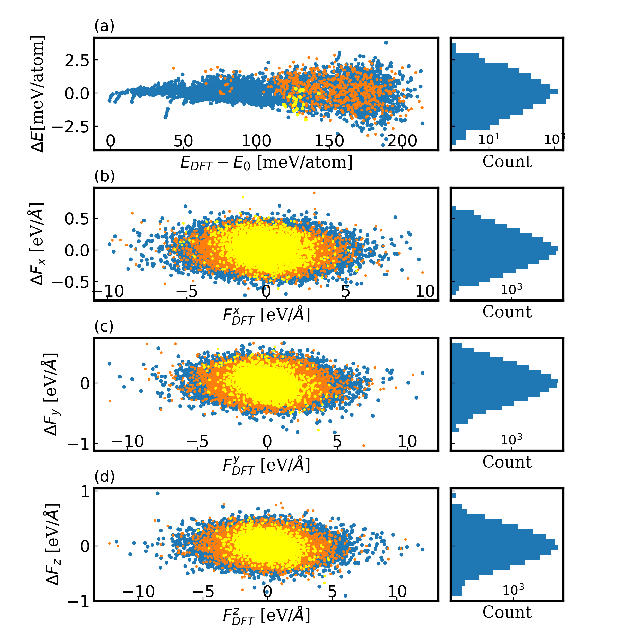
Figure 11: Error distribution of the energy model on the training set (Blue plots), test set (orange plots) and extra test set (yellow plots). $E_{\text{DFT}},F^{x,y,z}_{\text{DFT}}$ are the energy and force labels from the DFT data. $\Delta E,\Delta F_{x,y,z}$ are the difference between the model prediction and the label. $E_{0}$ is a constant used to shift the plot. (a) Left: The distribution of $\Delta E$ with respect to $E_{\text{DFT}}$. Right: The histogram of $\Delta E$ for the training set. (b-d) Left: The distribution of $\Delta F_{x,y,z}$ with respect to $F^{x,y,z}_{\text{DFT}}$. Right: The histogram of $\Delta F_{x,y,z}$ for the training set.

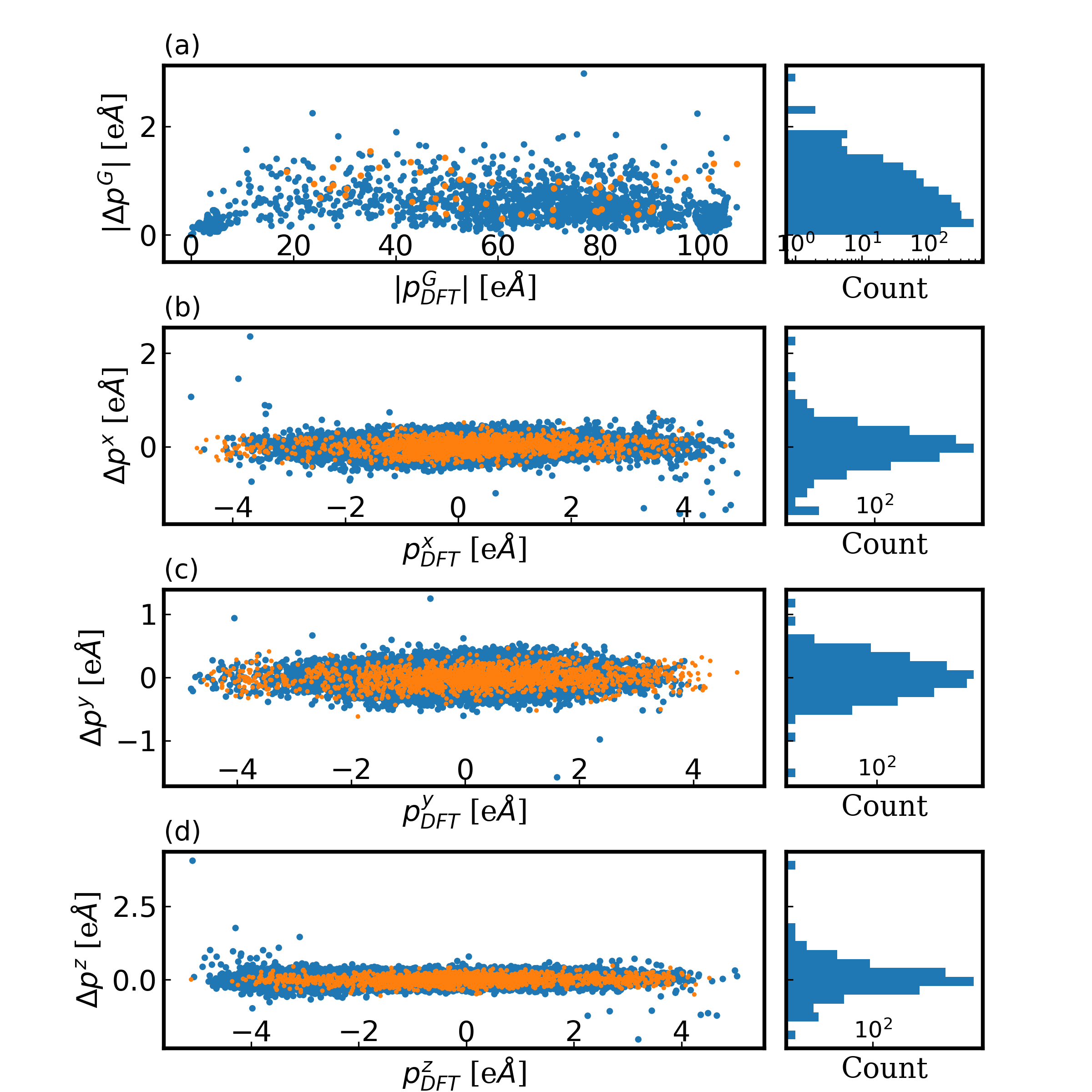
Figure 12: Error distribution of the dipole model on the training set (Blue plots) and test set (orange plots). $p^{G}_{\text{DFT}},p^{x,y,z}_{\text{DFT}}$ are the global and local dipole labels from the DFT data. $\Delta p^{G},\Delta p^{x,y,z}$ are the difference between the model prediction and the label. (a) Left: The distribution of the 2-norm of $\Delta p^{G}$ with respect to the 2-norm of $p^{G}_{\text{DFT}}$. Right: The histogram of $|\Delta p^{G}|$ for the training set. (b-d) Left: The distribution of $\Delta p^{x,y,z}$ with respect to $p^{x,y,z}_{\text{DFT}}$. Right: The histogram of $\Delta p^{x,y,z}$ for the training set.

By the end of the active learning procedure, we collect 5032 data points together with the energy, force and virial labels. 4432 data points are used to train the energy model. The other 600 data points are used for validation.

Fig. 11 (blue and orange plots) show the prediction accuracy of the energy model compared to the DFT data. The distribution of the error is roughly Gaussian. For the energy prediction, the standard deviation is around $1$meV per atom. For the force prediction, the standard deviation is around $0.25$eV$/$Å. Hence the energy model is very faithful to the current dataset. All the DFT data for training used $3\times 3\times 3$ supercell. To consider the generality of the model, we should test the model with DFT data with different supercells. To this end, we generate an extra test set consisting of twenty $4\times 4\times 4$ supercell atomic configurations, collected at NPT-MD simulations in the tetragonal phase. The error made by the energy model on this data set is shown in the yellow plots in Fig. 11. The error in the energy does not show any tendency to increase. The error in the force assumes similar Gaussian distribution as the previous dataset. Thus we conclude that our short-range energy model is faithful to the SCAN-based KS-DFT inside the temperature and pressure range specified by our dataset, with a deviation much smaller than the threshold of chemical accuracy.

In addition, we calculate the optimal lattice constants for structures with space group P4mm and Pm$\overline{3}$m respectively. The cubic lattice constant is $a_{\text{DP}}=3.93$Å, the same as the SCAN-DFT result. The tetragonal lattice constants are $a_{\text{DP}}=b_{\text{DP}}=3.86$Å and $c_{\text{DP}}=4.30$Å, slightly different from the SCAN-DFT results $a_{\text{DFT}}=b_{\text{DFT}}=3.846$Å and $c_{\text{DFT}}=4.393$Å. Further analysis shows the energy model yields $0.6$meV$/$atom difference between these two tetragonal structures while SCAN-DFT yields $1$meV$/$atom difference. This deviation is compatible with the error distribution of the energy model.

Dipole labels are added to the dataset after the training of the energy model. We compute the dipole labels for only part of the dataset because the entire dataset contains redundancy. Also, the generation of the dipole labels is much more expensive than the others. To determine which data point should be labeled, we train an ensemble of energy models with different reduced training sets. Then we compare the models trained with the reduced datasets to the productive energy model trained with the entire training set in terms of error distribution and structural relaxation. It turns out that a reduced dataset containing 1835 data points are already enough to produce an energy model with basically the same level of accuracy as the productive model. This is expected since the initial dataset contains a lot of similar atomic configurations from very short ab initio MD trajectories. Also, a lot of data points generated at the early stage of the learning process became redundant in the final dataset.

We generate dipole labels for the reduced training set consisting of 1835 data points. In addition, we generate a test set consisting of 61 data points collected using NPT-MD simulations in both cubic and tetragonal phase. The error distribution of the final dipole model is shown in Fig. 12. For the global dipole prediction, the standard deviation is roughly $1$eÅ for the $3\times 3\times 3$ supercell. The results suggest that the dipole model is highly accurate even for largely distorted structures. Meanwhile, the local dipole prediction is slightly worse. Within the scope of this work, we need only high accuracy on the global dipole which is rigorously defined by the modern theory of polarization. The local dipoles here are merely auxiliary variables.

For comparison, we also fit a linear model with static born charges as trainable parameters to all our dipole data. The standard deviation of the linear model on global dipole data is two times as large as our dipole model. For configurations near the two limit $|p_{\text{DFT}}^{G}|\approx 0$ and $|p_{\text{DFT}}^{G}|\approx 100e$Å the linear model gives outliers with error about three times the standard deviation. It implies the trained parameters effectively take the average of the cubic phase Born charges and the tetragonal phase Born charges.

Appendix C Technical Details of MD simulation

The MD simulations are carried out with the joint efforts of DeePMD-kit, LAMMPS and PLUMED Bonomi (2019); Tribello et al. (2014) with an additional package yix that implements the dipole model as the collective variables.

The results in Sec. III are obtained by unbiased MD simulations with the time step $\Delta t=0.5$fs and periodic boundary condition. The isothermal-isobaric condition is maintained by the MTK method  Martyna et al. (1994) with default parameters in LAMMPS. For each NPT-MD simulation, the total simulation time is around 1 nanosecond.

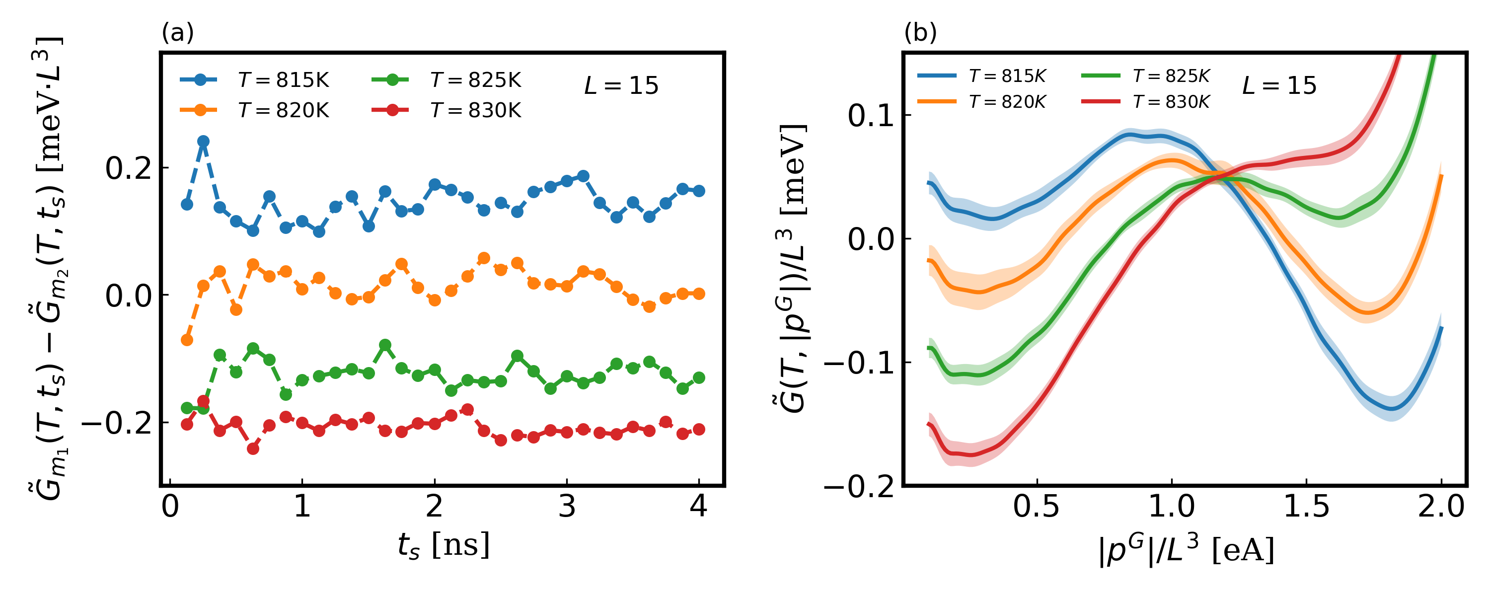
Figure 13: (a) The evolution of the difference between two free energy minima through the metadynamics simulation. (b) The average and the standard deviation of $\tilde{G}(T,|p^{G}|,t_{s})$ over $t_{s}>2$ns.

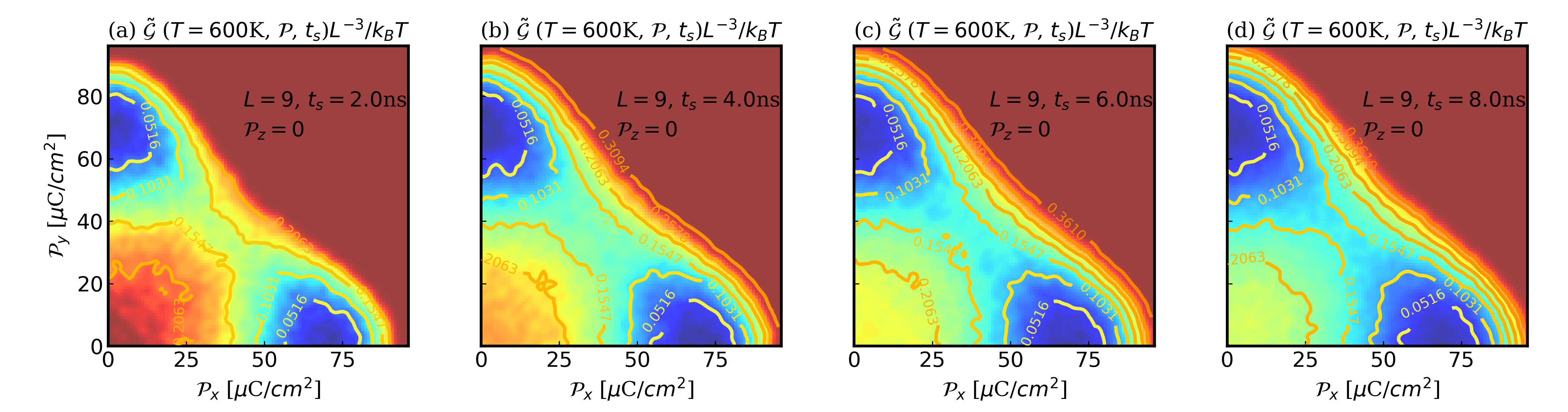
Figure 14: The colored representation of the $\mathcal{P}_{z}=0$ section of the intermediate free energy $\tilde{\mathcal{G}}(T,\mathcal{P},t_{s})$ in the units of $L^{3}k_{b}T$ for $T=600$K and $L=9$. For easier comparison, the free energy is shifted such that its minimum is zero.

The results in Sec. IV are obtained by biased MD simulations with the same time step, thermostats and barostats as the unbiased simulations. The phase space region explored by MD is controlled by the bias factor in well-tempered metadynamics.

The results in Sec. IV.1 were computed from well-tempered metadynamics simulations each lasting $4$ns. Let $\tilde{G}(T,|p^{G}|,t_{s})$ be the intermediate free energy shifted to zero mean for interval $|p^{G}|/L^{3}\in$ [$0.1$eÅ,$2$eÅ], computed at time $t_{s}$. We study the convergence of free energy by the relative height of the two basins in $\tilde{G}(T,|p^{G}|,t_{s})$. We write $\tilde{G}_{m_{1}}(T,t_{s})$ for the local free energy minimum associated to the paraelectric basin and $\tilde{G}_{m_{2}}(T,t_{s})$ for the ferroelectric basin. Fig. 13 (a) shows their difference for $T\in[815,820,825,830]$K. We observe that the fluctuation of the energy difference is under $0.1$meV$\cdot L^{3}$ after $t_{s}=2$ns and not improving further. Let $\tilde{G}(T,|p^{G}|)$ be the average of $\tilde{G}(T,|p^{G}|,t_{s})$ for equally spaced $t_{s}$ points over $t_{s}\in[2,4]$ns. Fig. 13 (b) gives a close look of $\tilde{G}(T,|p^{G}|)/L^{3}$ with standard deviation on the grid of $|p^{G}|/L^{3}$ (plotted as filled area) computed with the same set of $t_{s}$ points, from which a rough estimation of the stochastic error in free energy is of the order of $0.01$meV per unit cell.

The results in Sec. IV.2 are computed from well-tempered metadynamics simulations each lasting $8$ns. A typical convergence pattern represented by shifted intermediate free energy $\tilde{\mathcal{G}}(T,\mathcal{P},t_{s})$ is illustrated in Fig. 14.

References

- Resta and Vanderbilt (2007) R. Resta and D. Vanderbilt, “Theory of polarization: A modern approach,” in Physics of Ferroelectrics: A Modern Perspective (Springer Berlin Heidelberg, Berlin, Heidelberg, 2007) pp. 31–68.
- Marzari et al. (2012) N. Marzari, A. A. Mostofi, J. R. Yates, I. Souza, and D. Vanderbilt, Rev. Mod. Phys. 84, 1419 (2012).
- Zhang et al. (2017) Y. Zhang, J. Sun, J. P. Perdew, and X. Wu, Phys. Rev. B 96, 035143 (2017).
- Zhong et al. (1994) W. Zhong, D. Vanderbilt, and K. M. Rabe, Phys. Rev. Lett. 73, 1861 (1994).
- Zhong et al. (1995) W. Zhong, D. Vanderbilt, and K. M. Rabe, Phys. Rev. B 52, 6301 (1995).
- Waghmare and Rabe (1997) U. V. Waghmare and K. M. Rabe, Phys. Rev. B 55, 6161 (1997).
- Nishimatsu et al. (2008) T. Nishimatsu, U. V. Waghmare, Y. Kawazoe, and D. Vanderbilt, Phys. Rev. B 78, 104104 (2008).
- Tinte et al. (2003) S. Tinte, J. Íñiguez, K. M. Rabe, and D. Vanderbilt, Phys. Rev. B 67, 064106 (2003).
- Srinivasan et al. (2003) V. Srinivasan, R. Gebauer, R. Resta, and R. Car, AIP Conference Proceedings 677, 168 (2003).
- Tinte et al. (1999) S. Tinte, M. G. Stachiotti, M. Sepliarsky, R. L. Migoni, and C. O. Rodriguez, Journal of Physics: Condensed Matter 11, 9679 (1999).
- Goddard et al. (2002) W. A. Goddard, Q. Zhang, M. Uludogan, A. Strachan, and T. Cagin, AIP Conference Proceedings 626, 45 (2002).
- Grinberg et al. (2002) I. Grinberg, V. R. Cooper, and A. M. Rappe, Nature 419, 909 (2002).
- Brown (2009) I. D. Brown, Chemical Reviews 109, 6858 (2009).
- Liu et al. (2013) S. Liu, I. Grinberg, H. Takenaka, and A. M. Rappe, Phys. Rev. B 88, 104102 (2013).
- Ghosez and Junquera (2022) P. Ghosez and J. Junquera, Annual Review of Condensed Matter Physics 13, 325 (2022).
- Zhang et al. (2018a) L. Zhang, J. Han, H. Wang, R. Car, and W. E, Phys. Rev. Lett. 120, 143001 (2018a).
- Behler and Parrinello (2007) J. Behler and M. Parrinello, Phys. Rev. Lett. 98, 146401 (2007).
- Zhang et al. (2020a) L. Zhang, M. Chen, X. Wu, H. Wang, W. E, and R. Car, Phys. Rev. B 102, 041121 (2020a).
- Wu et al. (2021a) J. Wu, Y. Zhang, L. Zhang, and S. Liu, Phys. Rev. B 103, 024108 (2021a).
- Zhang et al. (2021) L. Zhang, H. Wang, R. Car, and W. E, Phys. Rev. Lett. 126, 236001 (2021).
- Tang et al. (2020) L. Tang, Z. J. Yang, T. Q. Wen, K. M. Ho, M. J. Kramer, and C. Z. Wang, Phys. Chem. Chem. Phys. 22, 18467 (2020).
- Yang et al. (2021) M. Yang, T. Karmakar, and M. Parrinello, Phys. Rev. Lett. 127, 080603 (2021).
- Lu et al. (2021a) D. Lu, H. Wang, M. Chen, L. Lin, R. Car, W. E, W. Jia, and L. Zhang, Computer Physics Communications 259, 107624 (2021a).
- Dawber et al. (2005) M. Dawber, K. M. Rabe, and J. F. Scott, Rev. Mod. Phys. 77, 1083 (2005).
- Wu et al. (2021b) J. Wu, L. Bai, J. Huang, L. Ma, J. Liu, and S. Liu, Phys. Rev. B 104, 174107 (2021b).
- Gigli et al. (2021) L. Gigli, M. Veit, M. Kotiuga, G. Pizzi, N. Marzari, and M. Ceriotti, arXiv preprint arXiv:2111.05129 (2021).
- Barducci et al. (2008) A. Barducci, G. Bussi, and M. Parrinello, Phys. Rev. Lett. 100, 020603 (2008).
- Sun et al. (2015) J. Sun, A. Ruzsinszky, and J. P. Perdew, Phys. Rev. Lett. 115, 036402 (2015).
- Paul et al. (2017) A. Paul, J. Sun, J. P. Perdew, and U. V. Waghmare, Phys. Rev. B 95, 054111 (2017).
- Blöchl (1994) P. E. Blöchl, Phys. Rev. B 50, 17953 (1994).
- Hamann et al. (1979) D. R. Hamann, M. Schlüter, and C. Chiang, Phys. Rev. Lett. 43, 1494 (1979).
- Zhang et al. (2022) L. Zhang, H. Wang, M. C. Muniz, A. Z. Panagiotopoulos, R. Car, and W. E, The Journal of Chemical Physics 156, 124107 (2022).
- Mabud and Glazer (1979) S. A. Mabud and A. M. Glazer, Journal of Applied Crystallography 12, 49 (1979).
- Zhang et al. (2018b) L. Zhang, J. Han, H. Wang, W. Saidi, R. Car, et al., Advances in Neural Information Processing Systems 31 (2018b).
- Rossetti and Maffei (2005) G. A. Rossetti and N. Maffei, Journal of Physics: Condensed Matter 17, 3953 (2005).
- Yoshida et al. (2009) T. Yoshida, Y. Moriya, T. Tojo, H. Kawaji, T. Atake, and Y. Kuroiwa, Journal of Thermal Analysis and Calorimetry 95, 675 (2009).
- Maffei and Rossetti (2004) N. Maffei and G. Rossetti, Journal of Materials Research 19, 827–833 (2004).
- Bhide et al. (1968) V. G. Bhide, M. S. Hegde, and K. G. Deshmukh, Journal of the American Ceramic Society 51, 565 (1968).
- Remeika and Glass (1970) J. Remeika and A. Glass, Materials Research Bulletin 5, 37 (1970).
- Nishino et al. (2020) R. Nishino, T. C. Fujita, F. Kagawa, and M. Kawasaki, Scientific Reports 10, 1 (2020).
- Dahl et al. (2009) Ø. Dahl, J. K. Grepstad, and T. Tybell, Journal of Applied Physics 106, 084104 (2009).
- Morita and Cho (2004) T. Morita and Y. Cho, Japanese Journal of Applied Physics 43, 6535 (2004).
- Deb et al. (1995) K. K. Deb, K. W. Bennett, and P. S. Brody, Journal of Vacuum Science & Technology A 13, 1128 (1995).
- Iijima et al. (1986) K. Iijima, Y. Tomita, R. Takayama, and I. Ueda, Journal of Applied Physics 60, 361 (1986).
- Bhide et al. (1962) V. Bhide, K. Deshmukh, and M. Hegde, Physica 28, 871 (1962).
- Íñiguez et al. (2001) J. Íñiguez, S. Ivantchev, J. M. Perez-Mato, and A. García, Phys. Rev. B 63, 144103 (2001).
- Geneste (2009) G. Geneste, Phys. Rev. B 79, 064101 (2009).
- Kumar and Waghmare (2010) A. Kumar and U. V. Waghmare, Phys. Rev. B 82, 054117 (2010).
- Nelmes et al. (1990) R. Nelmes, R. Piltz, W. Kuhs, Z. Tun, and R. Restori, Ferroelectrics 108, 165 (1990).
- Ravel et al. (1993) B. Ravel, E. A. Stern, Y. Yacobi, and F. Dogan, Japanese Journal of Applied Physics 32, 782 (1993).
- Sicron et al. (1994) N. Sicron, B. Ravel, Y. Yacoby, E. A. Stern, F. Dogan, and J. J. Rehr, Phys. Rev. B 50, 13168 (1994).
- Ravel et al. (1995) B. Ravel, N. Slcron, Y. Yacoby, E. A. Stern, F. Dogan, and J. J. Rehr, Ferroelectrics 164, 265 (1995).
- Datta et al. (2018) K. Datta, I. Margaritescu, D. A. Keen, and B. Mihailova, Phys. Rev. Lett. 121, 137602 (2018).
- Lu et al. (2021b) D. Lu, W. Jiang, Y. Chen, L. Zhang, W. Jia, H. Wang, and M. Chen, arXiv preprint arXiv:2107.02103 (2021b).
- Valsson and Parrinello (2014) O. Valsson and M. Parrinello, Phys. Rev. Lett. 113, 090601 (2014).
- Invernizzi et al. (2020) M. Invernizzi, P. M. Piaggi, and M. Parrinello, Phys. Rev. X 10, 041034 (2020).
- Gonzalo and Rivera (1971) J. Gonzalo and J. Rivera, Ferroelectrics 2, 31 (1971).
- Haun et al. (1987) M. J. Haun, E. Furman, S. Jang, H. McKinstry, and L. Cross, Journal of Applied Physics 62, 3331 (1987).
- Ducharme et al. (2000) S. Ducharme, V. M. Fridkin, A. V. Bune, S. P. Palto, L. M. Blinov, N. N. Petukhova, and S. G. Yudin, Phys. Rev. Lett. 84, 175 (2000).
- Nagarajan et al. (1999) V. Nagarajan, I. Jenkins, S. Alpay, H. Li, S. Aggarwal, L. Salamanca-Riba, A. Roytburd, and R. Ramesh, Journal of Applied Physics 86, 595 (1999).
- Pertsev et al. (2003) N. A. Pertsev, J. Rodriguez Contreras, V. G. Kukhar, B. Hermanns, H. Kohlstedt, and R. Waser, Applied Physics Letters 83, 3356 (2003).
- Car and Parrinello (1985) R. Car and M. Parrinello, Phys. Rev. Lett. 55, 2471 (1985).
- Giannozzi et al. (2009) P. Giannozzi, S. Baroni, N. Bonini, M. Calandra, R. Car, C. Cavazzoni, D. Ceresoli, G. L. Chiarotti, M. Cococcioni, I. Dabo, et al., Journal of Physics: Condensed Matter 21, 395502 (2009).
- Schlipf and Gygi (2015) M. Schlipf and F. Gygi, Computer Physics Communications 196, 36 (2015).
- Pizzi et al. (2020) G. Pizzi, V. Vitale, R. Arita, S. Blügel, F. Freimuth, G. Géranton, M. Gibertini, D. Gresch, C. Johnson, T. Koretsune, et al., Journal of Physics: Condensed Matter 32, 165902 (2020).
- Shirane et al. (1956) G. Shirane, R. Pepinsky, and B. C. Frazer, Acta Crystallographica 9, 131 (1956).
- Marzari and Vanderbilt (1998) N. Marzari and D. Vanderbilt, AIP Conference Proceedings 436, 146 (1998).
- Zhang et al. (2020b) Y. Zhang, H. Wang, W. Chen, J. Zeng, L. Zhang, H. Wang, and W. E, Computer Physics Communications 253, 107206 (2020b).
- Meyer and Vanderbilt (2002) B. Meyer and D. Vanderbilt, Phys. Rev. B 65, 104111 (2002).
- Zhang et al. (2019) L. Zhang, D.-Y. Lin, H. Wang, R. Car, and W. E, Phys. Rev. Materials 3, 023804 (2019).
- Plimpton (1995) S. Plimpton, Journal of Computational Physics 117, 1 (1995).
- Wang et al. (2018) H. Wang, L. Zhang, J. Han, and W. E, Computer Physics Communications 228, 178 (2018).
- Bonomi (2019) M. Bonomi, Nature Methods 16, 670 (2019).
- Tribello et al. (2014) G. A. Tribello, M. Bonomi, D. Branduardi, C. Camilloni, and G. Bussi, Computer Physics Communications 185, 604 (2014).
- (75) “DeepMD Plumed Module,” https://github.com/y1xiaoc/deepmd-plumed, accessed: 2021-07-10.
- Martyna et al. (1994) G. J. Martyna, D. J. Tobias, and M. L. Klein, The Journal of Chemical Physics 101, 4177 (1994).