Learning to Assemble Geometric Shapes

Abstract

Assembling parts into an object is a combinatorial problem that arises in a variety of contexts in the real world and involves numerous applications in science and engineering. Previous related work tackles limited cases with identical unit parts or jigsaw-style parts of textured shapes, which greatly mitigate combinatorial challenges of the problem. In this work, we introduce the more challenging problem of shape assembly, which involves textureless fragments of arbitrary shapes with indistinctive junctions, and then propose a learning-based approach to solving it. We demonstrate the effectiveness on shape assembly tasks with various scenarios, including the ones with abnormal fragments (e.g., missing and distorted), the different number of fragments, and different rotation discretization.

1 Introduction

We humans show an excellent ability in solving a shape assembly problem, e.g., tangram Slocum (2003), by analyzing a target object and its constituent parts. Machines, however, still fall short of the level of intelligence and often suffer from the combinatorial nature of assembly problems; the number of possible configurations drastically increases with the number of parts. Developing an effective learner that tackles the issue is crucial since the assembly problems are pervasive in science and engineering fields such as manufacturing processes, structure construction, and real-world robot automation Zakka et al. (2020).

There have been a large volume of studies Lodi et al. (2002) on different types of shape assembly or composition problems in a variety of fields such as biology Sanches and Soma (2009), earth science Torsvik (2003), archaeology Derech et al. (2018), and tiling puzzles Noroozi and Favaro (2016). When part shapes have neither distinct textures nor mating junctions, the assembly problem can be formulated as a combinatorial optimization problem, which aims to occupy a target object using candidate parts Coffman et al. (1996), such as tangram Slocum (2003). It is also related to the classic problem of bin packing Brown (1971); Goyal and Deng (2020), which is one of the representative problems in combinatorial optimization. Most previous related work, however, tackles shape assembly problems by exploiting mating patterns across parts, e.g., compatible junctions or textures of candidate parts. For example, a jigsaw puzzle problem is typically solved by comparing and matching patterns across fragments where each fragment contains a distinct pattern Cho et al. (2010). In general cases where such hints are unavailable (i.e., textureless parts and indistinctive junctions), assembling fragments becomes significantly more challenging.

Figure 1: Geometric shape assembly. Given randomly-partitioned fragments, it is challenging to assemble them into the target shape.

In this work we first introduce a simple yet challenging problem of assembly and then propose an efficient and effective learning-based approach to solving this problem. We split a two-dimensional target shape into multiple fragments of arbitrary polygons by a stochastic partitioning process Schumacher et al. (1969); Roy and Teh (2008) and ask an agent to assemble the target shape given the partitioned fragments while the original poses are hidden. Given a target object and a set of candidate fragments, the proposed model learns to select one of the fragments and place it into a right place. It is designed to process the candidate fragments in a permutation-equivariant manner and is capable of generalizing to cases with an arbitrary number of fragments.

Our experiments show that the proposed method effectively learns to tackle different assembly scenarios such as those with abnormal fragments, different rotation discretization, and colored textures, whereas a brute-force search, metaheuristic optimization Boussaïd et al. (2013), and Bayesian optimization approach Brochu et al. (2010) easily fall into a bad local optimum.

2 Problem Definition

Suppose that we are given textureless fragments with indistinctive junctions. Our goal is to sequentially assemble the given fragments, which is analogous to a tangram puzzle. Unlike an approach based on the backtracking method, which considers how remaining fragments will fit into unfilled area of the target shape, we attempt to solve such a problem with a learning-based method.

Geometric Shape Assembly.

Suppose that we are given a set of fragments $\mathcal{X}=\{\mathbf{x}_{i}\}_{i=1}^{N}$ and a target geometric shape $S$ on a space $\Phi$. In this work, we assume that both fragments and a target shape are defined on a two-dimensional space. We sequentially assemble those fragments into the target shape; at each step, a fragment $\mathbf{x}_{i}$ is sampled without replacement and placed on top of a current shape $\mathbf{c}$. Our goal is to reconstruct $S$ consuming all the fragments.

Shape Fragmentation Dataset.

We create a dataset by partitioning a shape into multiple fragments, which can be easily used to pose its inverse task, i.e., an assembly problem. Inspired by binary space partitioning algorithm Schumacher et al. (1969), we randomly split a target shape, create a set of random fragments for each target shape, choose the order of fragments, and rotate them at random. In particular, possible rotation is discretized to a fixed number of bins. After $K$ times of binary partitioning, we obtain $N=2^{K}$ fragments. The details are described in the supplementary material.

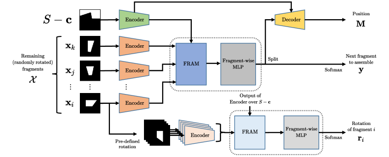
Figure 2: Overall architecture of the fragment assembly network, which includes all the components, e.g., a rotation branch, in Section 4.

3 Geometric Shape Assembly

To tackle the assembly problem, we propose a model that learns to select a fragment from candidates and place it on top of a current shape. The model is fed by two inputs:

1. remaining shape $S-\mathbf{c}$, which is a shape to assemble with the fragments excluding the fragments already placed;

2. a set of fragments $\mathcal{X}$, which consists of all candidates for the next assembly.

It then predicts which $\mathbf{x}_{i}\in\mathcal{X}$ should be used and where it should be placed on $\Phi$. We assemble all the fragments by iteratively running our model until no candidate remains.

To carefully make the next decision, the model needs to extract geometric information of the fragments and the target object, and also understand their relations. Our model is trained through the supervision obtained from shape fragmentation processes, which is expressed with a large number of episodes. Each episode contains the information about which fragment is the next and where the fragment is placed.

3.1 Fragment Assembly Networks

Our model, dubbed Fragment Assembly Network (FAN), considers a candidate fragment $\mathbf{x}_{i}$ in the context of the other candidates $\mathcal{X}\setminus\mathbf{x}_{i}$ and the remaining shape $S-\mathbf{c}$, and produces three outputs: (i) selection probability for $\mathbf{x}_{i}$, which implies how likely $\mathbf{x}_{i}$ is selected; (ii) placement probability map for $\mathbf{x}_{i}$, which means how likely each position is for $\mathbf{x}_{i}$; (optional, iii) rotation probability for $\mathbf{x}_{i}$, which indicates a bin index with respect to rotation angles. As shown in Figure 2, FAN contains two branches for the outputs, fragment selection network (i.e., FAN-Select) and fragment placement network (i.e., FAN-Pose). Both networks share many learnable parameters that are parts of encoders, Fragment Relation Attention Module (FRAM) and fragment-wise MLP. FRAM, inspired by a Transformer network Vaswani et al. (2017), captures the relational information between the fragments.

Fragment Selection.

FAN-Select is a binary classifier taking as inputs $\mathbf{x}_{i}$, $S-\mathbf{c}$, and $\mathcal{X}\setminus\mathbf{x}_{i}$:

$$y_{i}=\textrm{FAN-Select}\left(\mathbf{x}_{i};S-\mathbf{c},\mathcal{X}\setminus\mathbf{x}_{i}\right)\in\mathbb{R},$$ (1)

where $\mathbf{x}_{i}\in\mathcal{X}$. Since, in particular, Eq. (1) takes into account relationship between fragments with FRAM, it can choose the next fragment by considering the fragment candidates and remaining shape. Furthermore, the number of parameters in FAN does not depend on the number of fragments, which implies that the cardinality of $\mathcal{X}$ can be varied. This property helps our network to handle variable-length set of fragments. Note that $\mathbf{y}=[y_{i},\ldots,y_{|\mathcal{X}|}]\in\mathbb{R}^{|\mathcal{X}|}$.

Fragment Placement.

FAN-Pose determines the pose of $\mathbf{x}\in\mathcal{X}$ by predicting a probability map over pixels and a probability with respect to rotation angle bins:

$$\mathbf{M}_{i}(,\mathbf{r}_{i})=\textrm{FAN-Pose}\left(\mathbf{x}_{i};S-\mathbf{c},\mathcal{X}\setminus\mathbf{x}_{i},\mathcal{X}^{\prime}_{i}\right),$$ (2)

where $\mathcal{X}^{\prime}_{i}$ is a set of all possible pre-defined rotation of $\mathbf{x}_{i}$. Note that we simplify our problem with pre-defined discrete bins of rotation angles. This network is implemented as an encoder-decoder architecture with skip connections between them, in order to compute pixel-wise probabilities with convolution and transpose convolution operations. This structure reduces the number of parameters due to the absence of the last fully-connected layer. Note that $\mathbf{M}_{i}\in\mathbb{R}^{w\times h}$ and $\mathbf{r}_{i}\in\mathbb{R}^{b}$ where $b$ is the number of rotation angle bins.

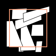
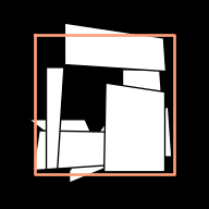
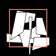
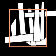
(a) Simulated annealing

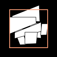
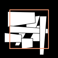
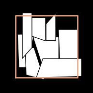
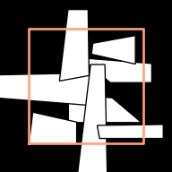
(b) Bayesian optimization

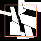
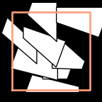
(c) V-GAN

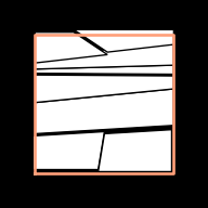
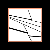
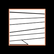
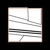
(d) Ours

Figure 3: Assembling results for Square.

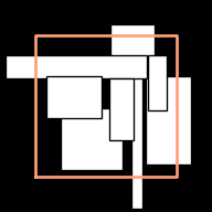
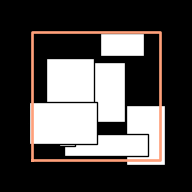
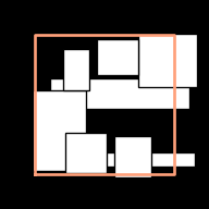
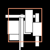
(a) Simulated annealing

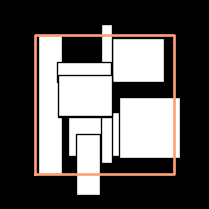
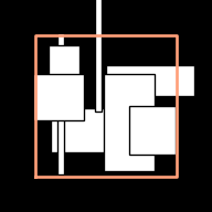
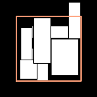
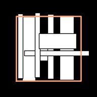
(b) Bayesian optimization

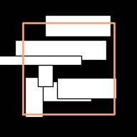
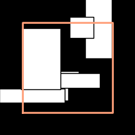
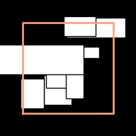
(c) V-GAN

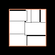
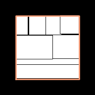
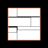
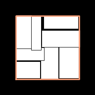
(d) Ours

Figure 4: Assembling results for Mondrian-Square.

Fragment Relation Attention Modules.

We suggest attention-based FRAM, which considers high-order relations between the remaining fragments using multi-head attentions Vaswani et al. (2017). Given $\mathbf{X}\in\mathbb{R}^{n_{1}\times d}$ and $\mathbf{Y}\in\mathbb{R}^{n_{2}\times d}$, multi-head attention is composed of multiple scaled dot-product attentions:

$$\textrm{DP}(\mathbf{Q},\mathbf{K},\mathbf{V}) =\sigma\left(\frac{\mathbf{Q}\mathbf{K}^{\top}}{\sqrt{d_{1}}}\right)\mathbf{V},$$ (3)

$$\textrm{MH}(\mathbf{X},\mathbf{Y},\mathbf{Y}) =[\textrm{DP}_{1},\ldots,\textrm{DP}_{h}]\mathbf{W}^{O},$$ (4)

where $\mathbf{Q}\in\mathbb{R}^{n_{1}\times d_{1}}$, $\mathbf{K}\in\mathbb{R}^{n_{2}\times d_{1}}$, $\mathbf{V}\in\mathbb{R}^{n_{2}\times d_{2}}$, $\textrm{DP}_{i}=\textrm{DP}(\mathbf{X}\mathbf{W}_{i}^{\mathbf{Q}},\mathbf{Y}\mathbf{W}_{i}^{\mathbf{K}},\mathbf{Y}\mathbf{W}_{i}^{\mathbf{V}})$, $\sigma$ is a softmax function, $h$ is the number of heads, and $\mathbf{W}^{O}\in\mathbb{R}^{hd_{2}\times d}$ is the parameters. To leverage the expression power of multi-head attention module, $\mathbf{X}$ and $\mathbf{Y}$ are projected by the different parameter sets $\mathbf{W}^{\mathbf{Q}}\in\mathbb{R}^{d\times d_{1}}$, $\mathbf{W}^{\mathbf{K}}\in\mathbb{R}^{d\times d_{1}}$, and $\mathbf{W}^{\mathbf{V}}\in\mathbb{R}^{d\times d_{2}}$.

Target Shape	Method	Cov@0.95	Cov@0.90	Cov	IoU	Time (sec.)
Square	SA	0.000	0.000	0.720	0.655	1,860
	BayesOpt	0.000	0.000	0.730	0.664	155
	V-GAN	0.000	0.000	0.720	0.562	$\boldsymbol{<}$ 1
	Ours	0.470	0.649	0.914	0.882	$\boldsymbol{<}$ 1
Pentagon	SA	0.000	0.000	0.697	0.581	1,854
	BayesOpt	0.000	0.000	0.710	0.660	149
	Ours	0.452	0.696	0.922	0.884	$\boldsymbol{<}$ 1
Hexagon	SA	0.000	0.000	0.711	0.608	1,846
	BayesOpt	0.000	0.000	0.727	0.674	153
	Ours	0.439	0.684	0.916	0.882	$\boldsymbol{<}$ 1

Table 1: Results on Square, Pentagon, and Hexagon shapes. Since the number of vertices in each polygon for Pentagon and Hexagon is different, V-GAN is not applicable for those cases.

Method	Cov@0.95	Cov@0.90	Cov	IoU	Time (sec.)
SA	0.000	0.000	0.761	0.671	153
BayesOpt	0.000	0.000	0.756	0.704	97
V-GAN	0.000	0.000	0.549	0.545	$\boldsymbol{<}$ 1
Ours	0.384	0.545	0.892	0.854	$\boldsymbol{<}$ 1

Table 2: Results on Mondrian-Square shape.

To express a set of the fragment candidates to a latent representation $\mathbf{h}$, we utilize the multi-head attention:

$$\mathcal{H} =\textrm{MH}(\mathcal{X},\mathcal{X},\mathcal{X})\in\mathbb{R}^{|\mathcal{X}|\times d},$$ (5)

$$\mathbf{h} =\textrm{MH}(\mathbf{1},\mathcal{H},\mathcal{H})\in\mathbb{R}^{d},$$ (6)

where $\mathbf{1}\in\mathbb{R}^{1\times d}$ is an all-ones matrix. Without loss of generality, Eq. (5) and Eq. (6) can take $\mathcal{X}$ (or $\mathcal{X}^{\prime}_{i}$) and $\mathcal{H}$, respectively. Moreover, Eq. (5) can be stacked by feeding $\mathcal{H}$ to the multi-head attention as an input, and Eq. (6) can be stacked in the similar manner. Note that $\mathbf{h}$ becomes $\mathbb{R}^{1\times d}$, but we can employ it as a $\mathbb{R}^{d}$-shaped representation. Additionally, FRAM includes a skip connection between an input and an output, in order to partially hold the input information.

FRAM is a generalization of global feature aggregation such as average pooling and max pooling across instances, so that it considers high-order interaction between instances and aggregates intermediate instance-wise representations (i.e., $\mathcal{H}$) with learnable parameters. In Section 4, we show that this module is powerful for assembling fragments via elaborate studies on geometric shape assembly.

The final output is determined by selecting the fragment with the index of maximum $y_{i}$: $i^{\star}=\operatornamewithlimits{\arg\max}_{i\in\{1,\ldots,|\mathcal{X}|\}}y_{i}$. After choosing the next fragment, its pose is selected through the maximum probability on $\mathbf{M}_{i^{\star}}$ (and $\mathbf{r}_{i^{\star}}$).

3.2 Training

We train our neural network based on the objective that combines losses for two sub-tasks, fragment selection, i.e., Eq. (7) and fragment placement, i.e., Eq. (8). Since we first choose the next fragment, and then determine the position and angle of the selected fragment, the gradient updates by the summation of two losses should be applied. Given a batch size $M$, the loss for the fragment selection part is

$$\mathcal{L}_{\textrm{select}}=\sum_{m=1}^{M}-\mathbf{t}_{m}^{\top}\log\sigma(\mathbf{y}_{m}),$$ (7)

where $\mathbf{t}_{m}$ is one-hot encoding of true fragment, each entry of $\mathbf{y}_{m}$ is computed by Eq. (1), and $\sigma$ is a softmax function.

Next, the objective for the fragment placement part is

$$\mathcal{L}_{\textrm{pose}} =-\sum_{m=1}^{M}\sum_{l=0}^{L}v(\textrm{max-p}_{2l}(\boldsymbol{\tau}_{m}))^{\top}\log v(\textrm{avg-p}_{2l}(\mathbf{M}_{m}))$$

$$\quad-\sum_{m=1}^{M}{\boldsymbol{\rho}}_{m}^{\top}\log\sigma(\mathbf{r}_{m}),$$ (8)

where $\boldsymbol{\tau}_{m}\in\mathbb{R}^{w\times h}$/${\boldsymbol{\rho}}_{m}\in\mathbb{R}^{r}$ are one-hot encodings of true position/true angle, $\mathbf{M}_{m}$ (and $\mathbf{r}_{m}$) are computed by Eq. (2), $L$ is the number of pooling operations, and max-p/avg-p/$v$ are functions for applying max-pooling/applying average-pooling/vectorizing a matrix. The subscript of pooling operations indicates the size of pooling and stride, and zero-sized pooling returns an original input. Moreover, the coefficients for balancing the objective functions should be multiplied to each term of the objectives; see the supplementary material.

4 Experimental Results

We show that the qualitative and quantitative results comparing to the three baselines for four target geometric shapes. We also provide studies on interesting assembly scenarios.

Details of Experiments.

As shown in Figure 1, we evaluate our method and existing methods on the following target objects: Square, Mondrian-Square, Pentagon, and Hexagon. Unless specified otherwise, we use 5,000 samples each of them is partitioned into 8 fragments using binary space partitioning and the number of rotation angle bins are set to 1, 4, or 20. We use 64%, 16%, and 20% of the samples for training, validation, and test splits, respectively. An assembly quality is calculated with coverage (Cov) and Intersection over Union (IoU).

$$\textrm{Cov}(\mathbf{c},S)=\frac{\textrm{area}(\mathbf{c}\cap S)}{\textrm{area}(S)}\ \ \textrm{and}\ \ \textrm{IoU}(\mathbf{c},S)=\frac{\textrm{area}(\mathbf{c}\cap S)}{\textrm{area}(\mathbf{c}\cup S)},$$ (9)

where $\mathbf{c}$ is an assembled shape and $S$ is a target shape.

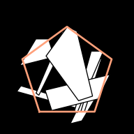
(a) Simulated annealing

(b) Bayesian optimization

(c) Ours

Figure 5: Assembling results for Pentagon.

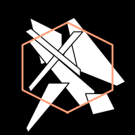
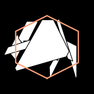
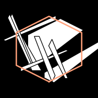
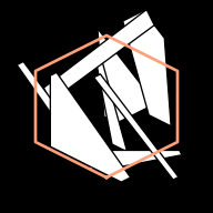
(a) Simulated annealing

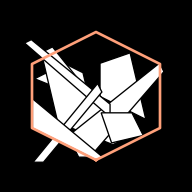
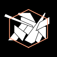
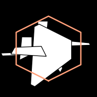
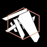
(b) Bayesian optimization

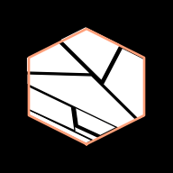
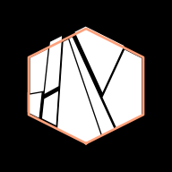
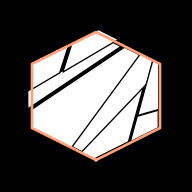
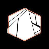
(c) Ours

Figure 6: Assembling results for Hexagon.

Since there exist no prior methods that specifically aim to tackle shape assembly of textureless fragments with indistinctive junctions, we compare ours with two classic optimization methods, simulated annealing Pincus (1970), Bayesian optimization Brochu et al. (2010), and a generative method using generative adversarial networks Li et al. (2020). The details can be found in the supplementary material.

4.1 Shape Assembly Experiments

Experiments in this section compare our approach to other baseline methods on the assembly of different target objects. The quantitative results on Square, Mondrian-Square, Pentagon, and Hexagon objects are summarized in Table 1. We find that our method consistently covers much more area than baselines within less time budget.

The qualitative results with randomly partitioned fragments from geometric shapes such as Square, Pentagon, and Hexagon are presented in Figure 3, Figure 5, and Figure 6. In Figure 4, the results with axis-aligned partitioning process, Mondrian-Square, is also presented.

V-GAN requires a fixed number of vertices for partitioned fragments, which is only applicable to Square and Mondrian-Square cases. Both SA and BayesOpt struggle to place fragments in the correct position, but many overlaps occur between fragments. They also consume longer time than our method in all experimental conditions. On the other hand, V-GAN consumes less time than other baseline methods while it significantly underperforms compared to other methods.

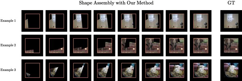
Figure 7: Assembling results for ImageNet examples with colored textures.

4.2 Elaborate Study & Ablation Study

We present interesting studies on Mondrian-Square objects, the number of fragments, abnormal fragments, rotation discretization, the effectiveness of FRAM, sequence sampling strategy, and scenarios with texture.

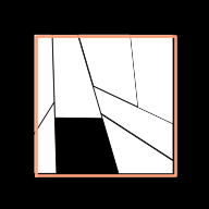
(a) Missing

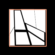
(b) Eroded

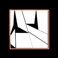
(c) Distorted

Figure 8: Scenarios with abnormal fragments.

#Frags	Target Shape	Cov@0.95	Cov@0.90	Cov	IoU
4 fragments	Square	0.972	0.989	0.991	0.962
	Pentagon	0.962	0.974	0.991	0.958
	Hexagon	0.940	0.976	0.989	0.956
16 fragments	Square	0.010	0.076	0.769	0.730
	Pentagon	0.024	0.108	0.797	0.755
	Hexagon	0.008	0.062	0.771	0.729

Table 3: Study on shape assemblies with 4 and 16 fragments.

Target Shape	Abnormal Type	Cov@0.95	Cov@0.90	Cov	IoU
Square	Missing	0.125	0.254	0.808	0.716
	Eroded	0.108	0.322	0.843	0.803
	Distorted	0.010	0.060	0.753	0.685
Pentagon	Missing	0.208	0.407	0.852	0.764
	Eroded	0.049	0.197	0.829	0.791
	Distorted	0.031	0.113	0.793	0.739
Hexagon	Missing	0.253	0.459	0.855	0.778
	Eroded	0.065	0.221	0.814	0.773
	Distorted	0.026	0.125	0.778	0.723

Table 4: Study on missing, eroded, and distorted scenarios.

Target Shape	#Bins	Cov@0.95	Cov@0.90	Cov	IoU
Square	4	0.010	0.017	0.670	0.622
	20	0.000	0.000	0.603	0.519
Pentagon	4	0.062	0.147	0.791	0.726
	20	0.000	0.000	0.604	0.515
Hexagon	4	0.009	0.046	0.731	0.676
	20	0.000	0.000	0.640	0.550

Table 5: Study on rotation discretization.

Method	Cov@0.95	Cov@0.90	Cov	IoU
w/o Aggregation	0.392	0.569	0.899	0.863
Max Pooling	0.390	0.563	0.893	0.856
Avg Pooling	0.431	0.580	0.899	0.863
w/ FRAM	0.470	0.649	0.914	0.882

Table 6: Study on feature aggregation methods.

Target Shape	Strategy	Cov@0.95	Cov@0.90	Cov	IoU
Square	Random	0.012	0.109	0.814	0.770
	$\nearrow$	0.470	0.649	0.914	0.882
Pentagon	Random	0.016	0.115	0.802	0.751
	$\nearrow$	0.452	0.696	0.922	0.884
Hexagon	Random	0.034	0.146	0.807	0.762
	$\nearrow$	0.439	0.684	0.916	0.882

Table 7: Study on sequence sampling strategy. $\nearrow$ indicates from bottom, left to top, right.

Axis-Aligned Space Partitioning.

To create a more challenging problem, we apply axis-aligned space partitioning in the shape fragmentation process. As shown in Figure 1, it generates similar rectangle fragments, which can puzzle our method. Nevertheless, our network successfully assembles the fragments given, as shown in Figure 4 and Table 2.

Number of Fragments.

As mentioned before, our model can be applied to the dataset that consists of a different number of fragments. Thus, we prepare a dataset, given the number of partitions $K=2$ or $K=4$. The results of our proposed model on the datasets with 4 fragments and 16 fragments of three geometric shapes are shown in Table 3. If the number of fragments is 4, it performs better than the circumstance with 8 fragments. On the contrary, a dataset with 16 fragments deteriorates the performance, but our method covers the target object with relatively small losses.

Abnormal Fragments.

We consider a particular situation to reconstruct a target object with missing, eroded, or distorted fragments, which can be thought of as the excavation scenario in archaeology; see Figure 8. We assume one fragment is missing, or four fragments are eroded or distorted randomly. We measure the performance of our method excluding the degradation from the ground-truth target object. Our methods outperform other methods as shown in Table 4.

Rotation Discretization.

To show the effects of rotation discretization, we test two bin sizes. As shown in Table 5, delicate discretization is more difficult than the case with a small bin size, which follows our expectation.

Effectiveness of FRAM.

It empirically validates the effectiveness of FRAM. As summarized in Table 6, FRAM outperforms other aggregation methods. The w/o aggregation model does not have a network for relations between fragments, and the other two models replace our FRAM to the associated aggregation methods among feature vectors.

Sequence Sampling Strategy.

As shown in Table 7, our sampling strategy that samples from bottom, left to top, right is effective compared to the random sampling technique that chooses the order of fragments based on the proximity of the fragments previously sampled.

Scenarios with Texture.

Our model is also able to handle a scenario with colored textures by allowing it to take RGB images. As shown in Figure 7, our method successfully assembles fragments with texture into the target object.

5 Discussion & Related Work

Compared to generic setting of jigsaw puzzle solvers Cho et al. (2010); Noroozi and Favaro (2016), our problem is more challenging as it involves textureless fragments and indistinctive junctions as well as arbitrary shapes and rotatable fragments. As presented in Table 1, the empirical results for Pentagon and Hexagon tend to be better than the results for Square. It implies that if a target shape becomes complicated and contains more information, the problem becomes more easily solvable. This tendency is also shown in the experiments with textures; see Figure 7.

The results with axis-aligned partitioning process, Mondrian-Square, is also presented in Table 2. The outcome by this process, which resembles the paintings by Piet Mondrian as shown in the second example of Figure 1, can be more difficult than the randomly partitioned shape, because fragment shapes and junction information are less expressive than arbitrary fragments. However the results show that our method is still more effective than the other baselines despite the performance loss, which implies that our method is able to select and place fragments although ambiguous choices exist; see Figure 4.

Unlike our random fragmentation, the approaches to solving a sequential assembly problem with fixed primitives Bapst et al. (2019); Kim et al. (2020); Chung et al. (2021) have been studied recently. However, they focus on constructing a physical object by assembling given unit primitives, and they utilize explicit supervision such as volumetric (or areal) comparisons and particular rewards.

6 Conclusion

In this paper, we have solved a two-dimensional geometric shape assembly problem. Our model, dubbed FAN, predicts the next fragment and its pose where fragments to assemble are given, with an attention-based module, dubbed FRAM. We showed that our method outperforms other baseline methods including simulated annealing, Bayesian optimization, and a learning-based adversarial network. Moreover, we evaluated our methods in diverse circumstances, such as novel assembly scenarios with axis-aligned space partitioning, degraded fragments, and colored textures.

Supplementary Material

In this material, we describe the detailed contents that supplement our main article.

S.1 Details of Shape Assembly

Algorithm s.1 Geometric Shape Assembly Procedure

0:  Fragments $\mathcal{X}=\{\mathbf{x}_{i}\}_{i=1}^{N}$ and a target shape $S$.

0:  Output shape $\mathbf{c}$.

1:  Initialize a current shape $\mathbf{c}$ on a space $\Phi$.

2:  while  $\mathcal{X}\neq\emptyset$ do

3:     Select $\mathbf{x}_{i}\in\mathcal{X}$ and place it on $\Phi$.

4:     Assemble $\mathbf{c}\leftarrow$ shape $\mathbf{c}$ updated by the placement of $\mathbf{x}_{i}$.

5:     Update $\mathcal{X}\leftarrow\mathcal{X}\setminus\mathbf{x}_{i}$.

6:  end while

7:  return $\mathbf{c}$

We provide the detailed procedure of shape assembly in Algorithm s.1.

S.2 Details of Shape Fragmentation

We present the procedure of shape fragmentation in Algorithm s.2.

Algorithm s.2 Shape Fragmentation

0:  A target shape $S$, the number of partitions $K$.

0:  Fragments partitioned $\mathcal{X}_{K}=\{\mathbf{x}_{i}\}_{i=1}^{2^{K}}$.

1:  Initialize a set of fragments $\mathcal{X}_{0}=\{S\}$.

2:  for $i=1,\ldots,K$ do

3:     Initialize $\mathcal{X}_{i}=\{\}$.

4:     for all $\mathbf{x}\in\mathcal{X}_{i-1}$ do

5:        Partition a fragment $\mathbf{x}$ to $\mathbf{x}_{+},\mathbf{x}_{-}$.

6:        Update $\mathcal{X}_{i}\leftarrow\mathcal{X}_{i}+\{\mathbf{x}_{+},\mathbf{x}_{-}\}$.

7:     end for

8:  end for

9:  Rotate all the fragments in $\mathcal{X}_{K}$ at random.

10:  return a set of fragments $\mathcal{X}_{K}$

(a) Partitioning 1

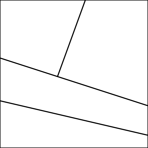
(b) Partitioning 2

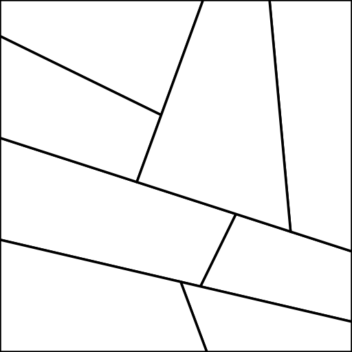
(c) Partitioning 3

Figure s.1: Fragmentation examples on Square by the number of partitions.

We divide a target geometric shape into fragments using a binary space partitioning algorithm Schumacher et al. [1969]. The number of fragments increases exponentially with the number of partitions. Some of partitioning examples are shown in Figure s.1.

We create a shape fragmentation dataset under two constraints that prevent generating small fragments. First, the hyperplane does not cross adjacent edges of the given polygon. Second, the position that the hyperplane will pass through is randomly selected between the range of $\pm$ 25$\%$ of edge length from the center of the edge. The dataset we use is composed of 5,000 samples.

Sequence Sampling Strategy.

As presented in Table 7, the consistency of assembling sequences in the dataset turns out to be crucial in training our network. If we employ the assembly order randomly determined in training our network, it performs significantly worse. To achieve better performance, we should select the next fragment that is adjacent to the fragments already chosen. As inspired by human assembling process Chazelle [1983], we determine the order of fragments from bottom, left to top, right by considering the center position of fragments in the target shape.

S.3 Details of Experiments

Our framework is implemented using TensorFlow Abadi et al. [2016]. We conduct the experiments on a Ubuntu 18.04 workstation with twelve Intel(R) Core i7-5930K CPU running at 3.50 GHz, 64 GB random access memory and NVIDIA Titan X (pascal) GPU.

To train our model with the objectives defined in the main article, we need to balance the terms in two objectives. Thus, we do our best to find the coefficients for these objectives. As a result, we scale up the term for determining the position of the next fragment by multiplying 1,000 and the term for a rotation probability by multiplying 10.

S.3.1 Baselines

We describe the details of baselines we employ in this paper.

Simulated annealing (SA).

Similar to our proposed method, SA Pincus [1970] iteratively selects and places one fragment such that IoU between the target object and assembled fragments is maximized. Thus, the optimization is repeated until the number of assembled fragments is equal to the given total budget.

Bayesian optimization (BayesOpt).

BayesOpt Brochu et al. [2010] is used to find the pose of given fragments by maximizing IoU between fragments and a target object. Similar to SA, the optimization is repeated in total of the number of fragments. We utilize the Bayesian optimization package Kim and Choi [2017] to implement this baseline.

LayoutGAN modified for vertex inputs (V-GAN).

It is a modification of Li et al. [2020]. Since LayoutGAN assumes that fragment shapes are always fixed and only finds their positions, we modify the generator structure to a neural network that takes fragment vertices as inputs and predicts center coordinates as their positions. Discriminator then makes real or fake decision based on adjusted vertex coordinates. Similar to GAN Goodfellow et al. [2014], it is trained via an adversarial training strategy.

S.3.2 Model Architecture

We introduce the model architecture for FAN including FRAM and V-GAN.

Network	Layer	Output Dimension
Generator	Reshape	64
	FC	128
	BatchNorm	128
	ReLU	128
	FC	64
	BatchNorm	64
	ReLU	64
	FC	32
	BatchNorm	32
	ReLU	32
	FC	16
Discriminator	Reshape	64
	FC	128
	ReLU	128
	Dropout 0.3	128
	FC	64
	ReLU	64
	Dropout 0.3	64
	FC	32
	ReLU	32
	Dropout 0.3	32
	FC	16

Table s.1: Architecture of V-GAN.

Network	Layer	Output Dimension
Encoder	Conv 2D, 16 ch., 3 $\times$ 3, stride 1, padding 1	128 $\times$ 128 $\times$ 16
	ReLU	128 $\times$ 128 $\times$ 16
	Dropout 0.1	128 $\times$ 128 $\times$ 16
	Conv 2D, 16 ch., 3 $\times$ 3, stride 1, padding 1	128 $\times$ 128 $\times$ 16
	ReLU	128 $\times$ 128 $\times$ 16
	Maxpool 2D, 2 $\times$ 2, stride 2, padding 0	64 $\times$ 64 $\times$ 16
	Conv 2D, 32 ch., 3 $\times$ 3, stride 1, padding 1	64 $\times$ 64 $\times$ 32
	ReLU	64 $\times$ 64 $\times$ 32
	Dropout 0.1	64 $\times$ 64 $\times$ 32
	Conv 2D, 32 ch., 3 $\times$ 3, stride 1, padding 1	64 $\times$ 64 $\times$ 32
	ReLU	64 $\times$ 64 $\times$ 32
	Maxpool 2D, 2 $\times$ 2, stride 2, padding 0	32 $\times$ 32 $\times$ 32
	Conv 2D, 64 ch., 3 $\times$ 3, stride 1, padding 1	32 $\times$ 32 $\times$ 64
	ReLU	32 $\times$ 32 $\times$ 64
	Dropout 0.2	64 $\times$ 64 $\times$ 32
	Conv 2D, 64 ch., 3 $\times$ 3, stride 1, padding 1	32 $\times$ 32 $\times$ 64
	ReLU	32 $\times$ 32 $\times$ 64
	Flatten	65,536
	Linear	256
	ReLU	256
Decoder	Linear	32,768
	ReLU	32,768
	Reshape	32 $\times$ 32 $\times$ 32
	ConvTranspose 2D, 32 ch., 2 $\times$ 2, stride 2, padding 2	64 $\times$ 64 $\times$ 32
	Conv 2D, 32 ch., 3 $\times$ 3, stride 1, padding 1	64 $\times$ 64 $\times$ 32
	ReLU	64 $\times$ 64 $\times$ 32
	Dropout 0.1	64 $\times$ 64 $\times$ 32
	Conv 2D, 32 ch., 3 $\times$ 3, stride 1, padding 1	64 $\times$ 64 $\times$ 32
	ReLU	64 $\times$ 64 $\times$ 32
	ConvTranspose 2D, 16 ch., 2 $\times$ 2, stride 2, padding 2	128 $\times$ 128 $\times$ 32
	Conv 2D, 32 ch., 3 $\times$ 3, stride 1, padding 1	128 $\times$ 128 $\times$ 16
	ReLU	128 $\times$ 128 $\times$ 16
	Dropout 0.1	128 $\times$ 128 $\times$ 16
	Conv 2D, 32 ch., 3 $\times$ 3, stride 1, padding 1	128 $\times$ 128 $\times$ 16
	ReLU	128 $\times$ 128 $\times$ 16
	Conv 2D, 1 ch., 1 $\times$ 1, stride 1, padding 0	128 $\times$ 128 $\times$ 1
MLP	Linear	256
	Batch normalization	256
	ReLU	256
	Linear	256
	Batch normalization	256
	ReLU	256
	Linear	1 or 256
FRAM
FRAM-Encoder	Encoder layer $\times$ 2 (including MHA. $\times$ 8)	256
FRAM-Decoder	Decoder layer $\times$ 2 (including MHA. $\times$ 8)	256

Table s.2: Architecture of FAN.

FAN.

FAN consists of FAN-Select that selects next fragment and FAN-Pose that predicts center coordinates of the chosen fragment. There exist 7 hyperparameters in FAN with 3 specifically in FRAM. Full details of the pipeline can be found in Table s.2. The default dimension of fully connected layer in the whole pipeline is fixed to 256 throughout the experiments. For the training, we use batch size of 32 and Adam optimizer Kingma and Ba [2015] for both FAN-Select and FAN-Pose with learning rate of $1\times 10^{-3}$ respectively. FAN-Select is a convolutional neural network (CNN) followed by FRAM including MLP block. FAN-Pose is convolutional encoder-decoder with MLP block followed by an additional fully-connected layer inserted in between. Each encoder for FAN-Pose and FAN-Select do not share the weights, and thus are trained with different loss. Our FRAM follows a similar setting of the original Transformer model Vaswani et al. [2017] with 2,048 hidden units and 8 attention heads.

V-GAN.

This model follows typical setup of generative adversarial network Goodfellow et al. [2014], having both generator and discriminator. Specifically, a generator takes fragment’s vertex coordinates as inputs and predicts center coordinates. Then fragment’s vertex coordinates are translated by predicted center coordinates. Next, a discriminator makes fake or real decision based on translated vertex coordinates. For training, we use batch size of 128 and Adam optimizer with learning rate of $1\times 10^{-4}$. The details of model is summarized in Table s.1.

S.4 Additional Discussion

Our proposed network can be viewed as a permutation-equivariant network, which satisfies $f(\pi([\mathbf{x}_{1},\ldots,\mathbf{x}_{n}]^{\top}))=\pi[f([\mathbf{x}_{1},\ldots,\mathbf{x}_{n}]^{\top})]$, where $f:\mathbb{R}^{n\times d}\to\mathbb{R}^{n\times d^{\prime}}$ is a neural network that outputs a set and $\pi$ is a permutation function along the first dimension. The work Guttenberg et al. [2016] suggests a permutational layer to handle the different inputs and does not depend on the specific order of inputs. The work of Zaheer et al. [2017] derives the necessary and sufficient conditions on permutation-equivariant networks. Moreover, an attention-based block for sets has been proposed Lee et al. [2019].

Furthermore, the number of learnable parameters does not depend on the dimensionality of $\mathbf{y}$ and the sizes of $\mathbf{M}_{i}$ and $\mathbf{r}_{i}$ for $i\in\{1,\ldots,|\mathcal{X}|\}$. As shown in Eq. (1) and Eq. (2), their outputs can handle variable-sized $\mathcal{X}$ and the order of $\mathcal{X}$ affects the order of the outputs, satisfying the permutation equivariance. The experimental results support that our method can learn these challenging scenarios.

References

- Abadi et al. [2016] Martín Abadi, Paul Barham, Jianmin Chen, Zhifeng Chen, Andy Davis, Jeffrey Dean, Matthieu Devin, Sanjay Ghemawat, Geoffrey Irving, Michael Isard, Manjunath Kudlur, Josh Levenberg, Rajat Monga, Sherry Moore, Derek G. Murray, Benoit Steiner, Paul Tucker, Vijay Vasudevan, Pete Warden, Martin Wicke, Yuan Yu, and Xiaoqiang Zheng. TensorFlow: A system for large-scale machine learning. In USENIX Symposium on Operating Systems Design and Implementation (OSDI), pages 265–283, Savannah, Georgia, USA, 2016.
- Bapst et al. [2019] Victor Bapst, Alvaro Sanchez-Gonzalez, Carl Doersch, Kimberly Lauren Stachenfeld, Pushmeet Kohli, Peter W. Battaglia, and Jessica B. Hamrick. Structured agents for physical construction. In Proceedings of the International Conference on Machine Learning (ICML), pages 464–474, Long Beach, California, USA, 2019.
- Boussaïd et al. [2013] Ilhem Boussaïd, Julien Lepagnot, and Patrick Siarry. A survey on optimization metaheuristics. Information Sciences, 237:82–117, 2013.
- Brochu et al. [2010] Eric Brochu, Vlad M. Cora, and Nando de Freitas. A tutorial on Bayesian optimization of expensive cost functions, with application to active user modeling and hierarchical reinforcement learning. arXiv preprint arXiv:1012.2599, 2010.
- Brown [1971] Arthur Robert Brown. Optimum packing and depletion. Macdonald and Co.; New York, American Elsevier, 1971.
- Chazelle [1983] Bernard Chazelle. The bottom-left bin-packing heuristic: An efficient implementation. IEEE Transactions on Computers, C-32(8):697–707, 1983.
- Cho et al. [2010] Taeg Sang Cho, Shai Avidan, and William T. Freeman. A probabilistic image jigsaw puzzle solver. In Proceedings of the IEEE International Conference on Computer Vision and Pattern Recognition (CVPR), pages 183–190, San Francisco, California, USA, 2010.
- Chung et al. [2021] Hyunsoo Chung, Jungtaek Kim, Boris Knyazev, Jinhwi Lee, Graham W. Taylor, Jaesik Park, and Minsu Cho. Brick-by-Brick: Combinatorial construction with deep reinforcement learning. In Advances in Neural Information Processing Systems (NeurIPS), volume 34, pages 5745–5757, Virtual, 2021.
- Coffman et al. [1996] Edward Grady Coffman, Michael Randolph Garey, and David Stifler Johnson. Approximation algorithms for bin packing: A survey. Approximation Algorithms for NP-hard Problems, pages 46–93, 1996.
- Derech et al. [2018] Niv Derech, Ayellet Tal, and Ilan Shimshoni. Solving archaeological puzzles. arXiv preprint arXiv:1812.10553, 2018.
- Goodfellow et al. [2014] Ian J. Goodfellow, Jean Pouget-Abadie, Mehdi Mirza, Bing Xu, David Warde-Farley, Sherjil Ozair, Aaron Courville, and Yoshua Bengio. Generative adversarial nets. In Advances in Neural Information Processing Systems (NeurIPS), volume 27, pages 2672–2680, Montreal, Quebec, Canada, 2014.
- Goyal and Deng [2020] Ankit Goyal and Jia Deng. PackIt: A virtual environment for geometric planning. In Proceedings of the International Conference on Machine Learning (ICML), pages 3700–3710, Virtual, 2020.
- Guttenberg et al. [2016] Nicholas Guttenberg, Nathaniel Virgo, Olaf Witkowski, Hidetoshi Aoki, and Ryota Kanai. Permutation-equivariant neural networks applied to dynamics prediction. arXiv preprint arXiv:1612.04530, 2016.
- Kim and Choi [2017] Jungtaek Kim and Seungjin Choi. BayesO: A Bayesian optimization framework in Python. https://bayeso.org, 2017.
- Kim et al. [2020] Jungtaek Kim, Hyunsoo Chung, Jinhwi Lee, Minsu Cho, and Jaesik Park. Combinatorial 3D shape generation via sequential assembly. In Neural Information Processing Systems Workshop on Machine Learning for Engineering Modeling, Simulation, and Design (ML4Eng), Virtual, 2020.
- Kingma and Ba [2015] Diederik P. Kingma and Jimmy Lei Ba. Adam: A method for stochastic optimization. In Proceedings of the International Conference on Learning Representations (ICLR), San Diego, California, USA, 2015.
- Lee et al. [2019] Juho Lee, Yoonho Lee, Jungtaek Kim, Adam Roman Kosiorek, Seungjin Choi, and Yee Whye Teh. Set Transformer: A framework for attention-based permutation-invariant neural networks. In Proceedings of the International Conference on Machine Learning (ICML), pages 3744–3753, Long Beach, California, USA, 2019.
- Li et al. [2020] Jianan Li, Jimei Yang, Aaron Hertzmann, Jianming Zhang, and Tingfa Xu. LayoutGAN: Synthesizing graphic layouts with vector-wireframe adversarial networks. IEEE Transactions on Pattern Analysis and Machine Intelligence, 2020.
- Lodi et al. [2002] Andrea Lodi, Silvano Martello, and Michele Monaci. Two-dimensional packing problems: A survey. European Journal of Operational Research, 141(2):241–252, 2002.
- Noroozi and Favaro [2016] Mehdi Noroozi and Paolo Favaro. Unsupervised learning of visual representations by solving jigsaw puzzles. In Proceedings of the European Conference on Computer Vision (ECCV), pages 69–84, Amsterdam, The Netherlands, 2016.
- Pincus [1970] Martin Pincus. Letter to the editor – a Monte Carlo method for the approximate solution of certain types of constrained optimization problems. Operations Research, 18(6):1225–1228, 1970.
- Roy and Teh [2008] Daniel M. Roy and Yee Whye Teh. The Mondrian process. In Advances in Neural Information Processing Systems (NeurIPS), volume 21, pages 1377–1384, Vancouver, British Columbia, Canada, 2008.
- Sanches and Soma [2009] Carlos Alberto Alonso Sanches and Nei Yoshihiro Soma. A polynomial-time DNA computing solution for the bin-packing problem. Applied Mathematics and Computation, 215(6):2055–2062, 2009.
- Schumacher et al. [1969] Robert Schumacher, Brigitta Brand, Maurice Gilliland, and Werner Sharp. Study for applying computer-generated images to visual simulation. Technical Report AFHRL-TR-69-14, Air Force Human Resources Laboratory, Air Force Systems Command, 1969.
- Slocum [2003] Jerry Slocum. Tangram: The World’s First Puzzle Craze. Sterling, 2003.
- Torsvik [2003] Trond H. Torsvik. The Rodinia jigsaw puzzle. Science, 300(5624):1379–1381, 2003.
- Vaswani et al. [2017] Ashish Vaswani, Noam Shazeer, Niki Parmar, Jakob Uszkoreit, Llion Jones, Aidan N. Gomez, Łukasz Kaiser, and Illia Polosukhin. Attention is all you need. In Advances in Neural Information Processing Systems (NeurIPS), volume 30, pages 5998–6008, Long Beach, California, USA, 2017.
- Zaheer et al. [2017] Manzil Zaheer, Satwik Kottur, Siamak Ravanbakhsh, Barnabas Poczos, Ruslan R. Salakhutdinov, and Alexander J. Smola. Deep sets. In Advances in Neural Information Processing Systems (NeurIPS), volume 30, pages 3391–3401, Long Beach, California, USA, 2017.
- Zakka et al. [2020] Kevin Zakka, Andy Zeng, Johnny Lee, and Shuran Song. Form2Fit: Learning shape priors for generalizable assembly from disassembly. In Proceedings of the International Conference on Robotics and Automation (ICRA), pages 9404–9410, Virtual, 2020.