Functional Network: A Novel Framework for Interpretability of Deep Neural Networks

Abstract

The layered structure of deep neural networks hinders the use of numerous analysis tools and thus the development of its interpretability. Inspired by the success of functional brain networks, we propose a novel framework for interpretability of deep neural networks, that is, the functional network. We construct the functional network of fully connected networks and explore its small-worldness. In our experiments, the mechanisms of regularization methods, namely, batch normalization and dropout, are revealed using graph theoretical analysis and topological data analysis. Our empirical analysis shows the following: (1) Batch normalization enhances model performance by increasing the global efficiency and the number of loops but reduces adversarial robustness by lowering the fault tolerance. (2) Dropout improves generalization and robustness of models by improving the functional specialization and fault tolerance. (3) The models with different regularizations can be clustered correctly according to their functional topological differences, reflecting the great potential of the functional network and topological data analysis in interpretability.

Keywords: Deep Neural Network, Interpretability, Functional Network, Topological Data Analysis, Graph Theoretical Analysis

1 Introduction

Deep neural networks are considered black-box models without a sufficient level of interpretability, which limits their wider applications and further development. Some studies focused on the structural information to explain them. However, many limitations exist: (1) Using only the structural information is insufficient to explain the performance differences of a model on diverse datasets. (2) The connections between neurons are preset and fixed, hindering the use of rich tools in network science. (3) The layered network structure only depicts the interactions between the neurons in the adjacent layers, rather than those in the same and non-adjacent layers. Hence, a new interpretable method with a general form that focuses on the network functions is urgently required.

Introducing the methods on brain function explanation in deep learning is feasible because many similarities exist between deep neural networks and the brain: (1) Deep learning is an artificial neural network technology inspired by the brain. (2) Reports show that similar coding mechanisms exist between them (Yang et al., 2019; Bi and Zhou, 2020). (3) Deep neural networks have been used as the computational models of the primate brain to explain its information processing (Yamins et al., 2014; Cadieu et al., 2014; Güçlü and van Gerven, 2015). An important method to understand the brain is to build a functional brain network that describes the statistical dependencies among neural activities of brain regions (McNabb et al., 2018; Beaty et al., 2018).

Motivated by the functional brain network, we propose a novel framework for interpretability of deep neural networks, that is, the functional network. This network can maintain practicability and provide insights into neuroscience. Given a deep neural network and a dataset, we record the output values of neurons when the model processes the dataset, compute the statistical dependencies among them, and construct the functional network by network binarization. In contrast to the structural network, the functional network depicts the functional interactions among neurons in the same layer and non-adjacent layers, in addition to the adjacent layers. By constructing the functional network, we introduce the powerful graph theoretical analysis (GTA) and topological data analysis (TDA) in the complex brain network analysis into interpretability of deep neural networks to capture the topological properties and high-order structures to explain how the models work. Furthermore, when a neural network processes diverse datasets, various functional networks are generated, and the variations in the functional networks can be utilized to explain the performance differences.

In this work, we partly reveal the mechanisms of the fully connected network (FCN). The results show that, similar to the functional brain network, the functional network of FCNs is a small-world network. This result suggests that deep neural networks have a similar functional organization to the brain, in which information transmits efficiently at a low cost. As an application of the functional network, we quantitatively analyze the effects of commonly used regularization techniques, namely, batch normalization and dropout, using graph theoretical and topological methods and explain how the methods work. Moreover, according to the topological differences between functional networks, the models with different regularizations can be correctly clustered. These findings demonstrate that the functional network can not only provide explanations for deep neural networks but also evaluate the models in practice.

2 Related Works

In this section, we introduce the previous works on interpretability of deep neural networks, particularly those using TDA, and the functional brain network in neuroscience.

Interpretability of Deep Neural Networks In recent years, interpretability of deep learning has attracted increasing attention from researchers. Several methods have been reported to address this issue, such as the extraction of logical rules or decision trees (Boz, 2002; Nayak, 2009), the interpretation for the semantics of neurons or convolutional layers (Bau et al., 2017; Dalvi et al., 2019; Zeiler and Fergus, 2014), the local perturbation-based explanations (Štrumbelj et al., 2009; Ribeiro et al., 2016; Akula et al., 2020), the prototype selection (Bien and Tibshirani, 2011; Kim et al., 2014), and the generalization capability or complexity measures (Rieck et al., 2019; Zhang et al., 2021; Raghu et al., 2017). However, some disadvantages exist in the previous works. For instance, the prototype selection and semantic interpretation only focus on the single data or feature and cannot provide a global understanding. Moreover, the rule extraction is only appropriate for deep neural networks with few neurons. Functional networks can overcome these shortcomings and explain the network mechanisms globally from the perspective of the functions of neurons.

TDA and Interpretability Recently, several attempts have been made to apply TDA to study interpretability of deep learning. Naitza et al. investigated the changes of data topology in the working process of FCNs and found that FCNs work by simplifying data topology until it becomes linearly separable (Naitzat et al., 2020). Rieck et al. proposed neural persistence to estimate the structure complexity and generalization ability using the zero-dimensional topological features (Rieck et al., 2019). Watanabe et al. extracted the one-dimensional topological structure features to investigate the inner representations of FCNs (Watanabe and Yamana, 2021). These studies indicated that TDA can extract high-order topological information to explain neural networks. However, some methods only use the structural information of the deep neural network and are not combined with data and tasks (Rieck et al., 2019; Watanabe and Yamana, 2021). Some approaches are only applicable to the model with a small number of neurons (Naitzat et al., 2020). In our work, TDA for the functional network depicts the functional organization of a deep neural network and evaluates its topological properties globally.

Functional Brain Network Analysis Using non-invasive brain-observation technologies, such as fMRI, researchers can record the neural activities of brain regions, calculate the statistical dependencies among them as the functional connectivities, and model the brain as a sparse binary graph, called the functional brain network. The nodes represent brain regions, and the edges represent functional connectivities. GTA is a powerful mathematical tool in complex brain network analysis. GTA is used to describe and interpret brain changes during development (Menon, 2013), reveal learning mechanisms (Bassett et al., 2011, 2015), understand the pathogenesis of brain diseases and provide imaging biomarkers for diagnosis (Rudie et al., 2013; McNabb et al., 2018). Nevertheless, the graph can only model the binary relation and cannot model the multivariate relation in the brain. Selecting a favorable threshold for functional network construction is difficult. To address these problems, TDA, a rapidly developing mathematical tool based on algebraic topology, is employed to assess the brain structures (Singh et al., 2008; Petri et al., 2014), distinguish the brain states (Billings et al., 2021), discover spatial coding principles (Dabaghian et al., 2012), and study the pathogenesis of diseases (Shnier et al., 2019). Those studies show that TDA can effectively describe higher-order interactions and capture more topological information about functional organizations in the brain without selecting a threshold. In our work, we used GTA and TDA to reveal the mechanisms of deep neural networks.

3 Background: Graph Theoretical Analysis and Topological Data Analysis

3.1 GTA

Graph theory is the main mathematical tool in the field of complex network analysis. A complex network is modeled as a binary graph model $G(V,E)$, where $V=\{v_{i}\}_{1\leq i\leq n}$ is the node set and $E=\{e_{k}|e_{k}=(v_{i},v_{j}),v_{i},v_{j}\in V\}_{1\leq k\leq m}$ is the edge set. Edges can be weighted, and the weight function $\psi:E\rightarrow\mathbb{R}^{+}\cup\{0\}$ maps the edge $e_{k}=(v_{i},v_{j})$ to a non-negative weight $w_{ij}$. $W=\{w_{ij}|w_{ij}=\psi(e_{k}),e_{k}=(v_{i},v_{j})\in E\}$ is the weight set. $G(V,E,W)$ is called a weighted graph. Referring to the textbook (Balakrishnan and Ranganathan, 2012), some properties of a binary graph $G(V,E)$ are briefly introduced as follows:

Density: The density of $G(V,E)$ is the ratio of the number of edges in $E$ to the maximum possible number of edges,

$$density=\frac{2m}{n(n-1)}$$ (1)

where $n$ and $m$ are the number of nodes and edges in $G$, respectively. In complex network analysis, the density has an important impact on other network properties.

Average shortest path length: The shortest path length $l_{ij}$ between nodes $v_{i}$ and $v_{j}$ is defined as the shortest length of all paths between $v_{i}$ and $v_{j}$. This length can also be called the distance between the two nodes. The average shortest path length $L$ of $G(V,E)$ is the average value of the shortest path lengths between all node pairs:

$$L=\frac{1}{n(n-1)}\sum_{v_{i},v_{j}\in V,i\neq j}l_{ij}$$ (2)

Global efficiency:The global efficiency $E_{global}$ of $G(V,E)$ is as follows:

$$E_{global}=\frac{1}{n(n-1)}\sum_{v_{i},v_{j}\in V,i\neq j}\frac{1}{l_{ij}}$$ (3)

where $l_{ij}$ is the shortest path length between nodes $v_{i}$ and $v_{j}$.

Clustering coefficient: For a node $v_{i}$, $\mathbb{S}_{i}=\{(v_{j},v_{k})|(v_{j},v_{k}),(v_{i},v_{j})\ and\ (v_{i},v_{k})\in E\}$ represents the edge set between its neighborhoods. The clustering coefficient $c_{i}$ of the node $v_{i}$ is defined as the ratio of the number of actual edges between its neighborhoods and the maximum possible number of edges between them:

$$c_{i}=\frac{2|\mathbb{S}_{i}|}{k_{i}(k_{i}-1)}$$ (4)

where $k_{i}$ is the number of the neighborhoods of $v_{i}$ and $|\mathbb{S}|$ is the number of actual edges between them. The average clustering coefficient $C$ of $G(V,E)$ is the average value of the clustering coefficients of all nodes:

$$C=\frac{1}{n}\sum_{v_{i}\in V}c_{i}$$ (5)

3.2 TDA

TDA is a rapidly developing mathematical tool based on algebraic topology, which can effectively extract the topological information of data. Please refer to (Edelsbrunner and Harer, 2009) for more details.

Simplicial homology: The simplicial complex is the core object of TDA. A $k$-simplex $\tau$ is the convex hull of $k+1$ vertices. A $0$-simplex is a vertex, a $1$-simplex is a line segment, and a $2$-simplex is a triangle. A face of $\tau$ is the convex hull of any subset of the $k+1$ vertices. A simplicial complex $K$ is a set of simplexes satisfied: (1) All faces of a simplex in $K$ are in $K$. (2) The intersection of two simplexes in $K$ is their common face. Simplicial homology uses homology groups to describe the topological invariants of a simplicial complex. The rank of its $k$-dimensional homology group is called the $k$-dimensional Betti number $\beta_{k}$ and represents the number of $k$-dimensional holes ($k$-holes). The Betti numbers $\beta_{0}$, $\beta_{1}$, and $\beta_{2}$ represent the numbers of connected components, loops, and voids contained in $K$, which is the simplification of topological information.

Persistent homology: Persistent homology was developed to characterize the topological information of real data with noise. The super-level filtration adapted in this study is defined as follows: Given a simplicial complex $K$ and a weighting function $\phi$ that maps the simplex $\tau$ in $K$ to a weight $w_{i}$, and the weight of $\tau$ must be less than or equal to the weights of its faces. When the value $\varepsilon$ is chosen, all the simplexes with weights greater than $\varepsilon$ form a simplicial complex $K_{i}$. Moreover, a simplicial complex sequence of $K$: $\emptyset=K_{0}\subseteq K_{1}\subseteq...\subseteq K_{m}=K$ is obtained by reducing the value $\varepsilon$.

In the filtration, a $k$-hole that generates at $\varepsilon_{i_{1}}$ and dies at $\epsilon_{i_{2}}$ can be represented by a point $(\epsilon_{i_{1}},\epsilon_{i_{2}})\in\mathbb{R}^{2}$. All points representing the $k$-holes are drawn on a two-dimensional plane, defined as a $k$-dimensional persistence diagram ($k$-PD) $D_{k}$, which describes the birth and death times of all $k$-holes. The $k$-dimensional Betti number sequence of $K$ can be induced from $D_{k}$, which is called the $k$-dimensional Betti curve $\beta_{k}(\varepsilon)$ (Dong et al., 2021). This Betti curve describes the topological invariant $\beta_{k}$ that persists across multiple scales.

4 Construction of Functional Networks

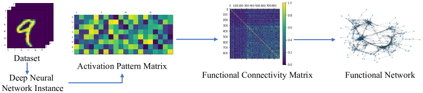
Figure 1: Flow chart of constructing the functional network for a given deep neural network.

In this section, we introduce the method for constructing the functional network of an FCN. As shown in Figure 1, the activation pattern matrix $\mathcal{A}$ is first generated to construct the functional network for a given FCN. Then, the functional connectivity matrix $\mathcal{F}$ is obtained by calculating the correlation matrix $\mathcal{R}$ according to the activation pattern matrix $\mathcal{A}$. Finally, the functional network $G$ is produced by binarizing $\mathcal{F}$. The details for generating the functional network are elucidated as follows.

Activation Pattern Matrix Generation Suppose a trained FCN model $\mathbb{M}$ with $l(l\geq 1)$ hidden layers and $n$ hidden neurons in total and a dataset $\mathbb{D}$ with $m$ data are given. First, data $d_{i}\in\mathbb{D}$ is inputted into $\mathbb{M}$, the output value of the $j^{th}$ hidden neuron is denoted as $a_{ij}$, and an activation pattern $(a_{i1},a_{i2},...,a_{in})$ is generated, which represents the information processing of $\mathbb{M}$ for $d_{i}$. The activation pattern matrix $\mathcal{A}$ is defined by considering all the data $d_{i}\in\mathbb{D}(i=1,2,\dots,m)$:

$$\mathcal{A}=(a_{ij})_{m\times n},1\leq i\leq m,1\leq j\leq n.$$ (6)

In the activation pattern matrix $\mathcal{A}$, the $j^{th}$ column vector is denoted as $A_{j}=[a_{1j},a_{2j},\cdots,a_{mj}]^{T}$, which represents the output of the $j^{th}$ hidden neuron. If the output vectors $A_{i}$ and $A_{j}$ ($i\neq j$) are statistically dependent, then the $i^{th}$ and $j^{th}$ neurons have functional synergy, which is called functional connectivity.

Functional Connectivity Matrix Construction The statistical dependency of two hidden neurons is calculated based on the activation pattern matrix $\mathcal{A}$. Many methods can be used to measure the statistical dependency between two variables, including Pearson correlation, partial correlation, and mutual information (Fornito et al., 2016). Compared with Pearson correlation, the estimation of partial correlation is difficult (Ryali et al., 2012) because of a large number of neurons in $\mathbb{M}$. In addition, the inaccurate estimation of mutual information limits its applications in practice (Daub et al., 2004). Consequently, we choose Pearson correlation to measure the degree of the linear relationship between two neurons (Heumann et al., 2016). The advantages of the Pearson correlation coefficient $r$ are threefold: low computational complexity, ranging from $[-1,1]$, and the clear significance, that is, the closer the absolute value is to 1, the stronger the linear relationship between two variables is.

To summarize the correlations between all possible pairs of neurons, the correlation matrix $\mathcal{R}$ of output values of hidden neurons is defined by the activation pattern matrix $\mathcal{A}$ as follows:

Definition 1 (Correlation Matrix)

Given an activation pattern matrix $\mathcal{A}$, the Pearson correlation coefficient $r_{ij}$ between the output values of the $i^{th}$ and $j^{th}$ hidden neurons is defined as follows:

$$r_{ij}=\frac{\sum_{k=1}^{m}(a_{ki}-\overline{a_{\star i}})(a_{kj}-\overline{a_{\star j}})}{\sqrt{\sum_{k=1}^{m}(a_{ki}-\overline{a_{\star i}})^{2}}\sqrt{\sum_{k=1}^{m}(a_{kj}-\overline{a_{\star j}})^{2}}},$$ (7)

where $\overline{a_{\star j}}=\frac{1}{m}\sum_{k=1}^{m}a_{kj}$ is the average output value of the $j^{th}$ hidden neuron. Then, the correlation matrix $\mathcal{R}=(r_{ij})_{n\times n}$ is formed by $r_{ij}$.

We take the absolute value of $r_{ij}$ as the strength of the functional connectivity between the $i^{th}$ and $j^{th}$ hidden neurons and assume that a neuron has no functional connectivity with itself. Accordingly, the functional connectivity matrix $\mathcal{F}$ is defined as follows:

Definition 2 (Functional Connectivity Matrix)

Given a correlation matrix $\mathcal{R}=(r_{ij})_{n\times n}$, the functional connectivity matrix $\mathcal{F}=(f_{ij})_{n\times n}$ is defined as follows:

$$f_{ij}=\begin{cases}|r_{ij}|,&\text{if }i\neq j,\\ 0,&\text{if }i=j;\end{cases}1\leq i,j\leq n,$$ (8)

where $f_{ij}$ is the strength of the functional connectivity between the $i^{th}$ and $j^{th}$ hidden neurons, $0\leq f_{ij}\leq 1$.

The functional connectivity matrix $\mathcal{F}$ represents a weighted complete graph $F(V,E_{f},W_{f})$. Here, $V=\{v_{1},v_{2},\dots,v_{n}\}$ is the node set, and the node $v_{j}$ represents the $j^{th}$ hidden neuron in $\mathbb{M}$. $E_{f}=\{e_{1},e_{2},\dots,e_{n(n-1)/2}\}$ is the edge set, and the edge $e_{k}=(v_{i},v_{j})=(v_{j},v_{i})$ represents the functional connectivity between the $i^{th}$ and $j^{th}$ hidden neurons. Moreover, a weight function $\psi:E_{f}\rightarrow\mathbb{R}^{+}\cup\{0\}$ is induced from $F$ that maps the edge $e_{k}=(v_{i},v_{j})$ to a non-negative weight: $\psi(e_{k})=w_{k}=f_{ij}$. $W_{f}=\{w_{k}|\psi(e_{k})=w_{k},e_{k}\in E_{f}\}$ is the weight set. $F(V,E_{f},W_{f})$ encodes the statistical dependencies between the hidden neurons in $\mathbb{M}$. However, considering all functional connectivities is inefficient. By binarizing $F$, the graph’s structure is simplified, and the functional network is generated.

Functional Network Formation In neuroscience, network binarization is a common method to construct the functional brain network from a weighted complete graph. We used it to extract the functional network $G(V,E)$ from $F(V,E_{f},W_{f})$. First, the maximum spanning tree $T(V,E_{t},W_{t})$ of $F(V,E_{f},W_{f})$, which is the spanning tree with a maximum weight of $F$, is constructed as the main node-edge structure of $G(V,E)$ to ensure its connectivity. This spanning tree contains all the nodes and $n-1$ edges with the density of $2/n$, which is the ratio of the number of edges in the graph to that of the corresponding complete graph. $E_{t}$ is a subset of $E_{f}$, and $W_{t}=\{w_{k}|\psi(e_{k})=w_{k},e_{k}\in E_{t}\}$ is the weight set. Then, more edges are required to be added to it because the tree structure cannot completely depict the interactions among neurons. One of the alternatives is to empirically select a density threshold $d$ for $G(V,E)$, which satisfies $2/n\leq d\leq 1$. This selection means that the functional network $G(V,E)$ should contain $[d\times n\times(n-1)/2]$ edges. We construct $G(V,E)$ as follows:

Definition 3 (Functional Network)

Given a density $d$ and a weighted complete graph $F(V,E_{f},W_{f})$, let $E_{t}$ be the edge set of its maximum spanning tree. The weights of edges in the $E_{f}\setminus E_{t}$ are sorted in a non-ascending order: $w^{\prime}_{1}\geq w^{\prime}_{2}\geq...\geq w^{\prime}_{(n-1)(n-2)/2}$, and the edge set of the functional network is defined as

$$E=E_{t}\cup\{e_{k}\in E_{f}\ |\ \psi(e_{k})\geq w^{\prime}_{\left[d\times n\times(n-1)/2\right]-(n-1)}\}.$$ (9)

The binary graph $G(V,E)$ is called the functional network.

The selection of $d$ determines the structure of $G(V,E)$, but a unified density selection method does not exist. In neuroscience, many studies show that the sparse network can better manifest the differences of the functional organization (Varoquaux et al., 2013; Lv et al., 2013). Therefore, we empirically selected multiple small densities for the network binarization in practical applications.

In summary, the defined functional network $G(V,E)$ depicts the functional interaction between hidden neurons in the neural network globally, regardless of whether physical connectivities exist, breaking the fixed connection relationships between them. By adopting the functional network, GTA and TDA can be used to capture the functional organization of deep neural networks and explain and distinguish various models based on their functional differences, supported by the results of the following experiments.

5 Experiments

In this section, we demonstrate the utility and significance of the functional network for FCNs through some experiments. First, we explore the small-worldness of the functional network, which is observed on the functional brain network in the studies (Young et al., 2000; Stam, 2004). Second, we investigate the impact of two commonly used regularization techniques and explain how they work using GTA and TDA. Finally, unsupervised clustering is performed according to the topological differences between the functional networks to demonstrate the effectiveness of TDA in evaluating and distinguishing the FCNs. The Fashion-MNIST (Xiao et al., 2017), MNIST (Deng, 2012), and CIFAR-10 (Krizhevsky, 2009) datasets are employed in all experiments.

5.1 Datasets and Models

The MNIST, Fashion-MNIST, and CIFAR-10 datasets were employed in the experiments. The contents of the MNIST, Fashion-MNIST, and CIFAR-10 datasets are $28\times 28$ grayscale handwritten digits, $28\times 28$ grayscale fashion products images, and $32\times 32$ color photographs, respectively (Deng, 2012; Xiao et al., 2017; Krizhevsky, 2009).

We used leaky ReLU activation functions with the negative slope of 0.01 in the hidden layers and the Adam optimizer with a learning rate of $3\times 10^{-4}$. Each deep neural network was trained for 100 epochs with a batch size of 64. Tables 5.1 and 2 show the architecture of the deep neural network trained in the small-world and regularization experiments, respectively.

Table 1: Architectures of the FCNs trained in the small-world experiments.

Dataset	Number of hidden layers	Architecture
MNIST	2	[300,100],[300,300]
	3	[300,300,100], [300,300,300]
Fashion-MNIST	2	[400,200],[400,400]
	3	[400,400,200],[400,400,400]
CIFAR-10	2	[500,300],[500,500]
	3	[500,500,300],[500,500,500]

Table 2: Architectures of the FCN trained in the regularization experiments.

Dataset	Number of hidden layers	Architecture
Fashion-MNIST	2	[400,200],[400,400]
	3	[400,400,200],[400,400,400]
MNIST	2	[300,100]
	3	[300,300,300]
CIFAR-10	2	[500,300]
	3	[500,500,300]

5.2 Small-World Experiments

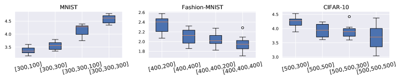
Figure 2: Box plots for the small-world coefficients of the functional networks for the FCNs with different architectures.

The network with a large average clustering coefficient and a small average shortest path length is called a small-world network. This property is called the small-worldness, which can be measured by the small-world coefficient $\sigma$ (Humphries and Gurney, 2008):

$$\sigma=\frac{C_{real}/C_{random}}{L_{real}/{L_{random}}},$$ (10)

where $C_{real}$ and $C_{random}$ mean the average clustering coefficient of the real network and its equivalent random network, respectively; $L_{real}$ and $L_{random}$ mean the average shortest path length of the real network and its equivalent random network, respectively. If $\sigma$ is greater than 1, then the real network is deemed a small-world network. The larger $\sigma$ is, the more significant the small-worldness is.

Previous studies (Young et al., 2000; Stam, 2004) suggested that the functional brain network is a small-world network and any two brain regions only have a small number of intermediate steps to connect. This functional organization improves the efficiency of global information transmission in the brain and reflects the optimal organization pattern for information processing (Strogatz, 2001; Dodel et al., 2002; Eguíluz et al., 2005). Analogously, a worthy question arises to explore the existence of the small-worldness in the functional network of deep neural networks. To study it, we used the FCNs trained on three datasets. For each dataset, we trained four groups of FCNs with different architectures, as shown in Table 5.1 in Section 5.1. Each group includes 10 FCNs with only the initial values diverse. Then, we constructed their functional networks with a density of $2.5\%$, calculated the small-world coefficients $\sigma$, and illustrated the results in Figure 2.

For the FCNs trained on the MNIST and CIFAR-10 datasets, the small-world coefficients of all functional networks are between 3.0 and 5.0, whereas for the FCNs trained on the Fashion-MNIST dataset, the values are between 1.6 and 2.6. The small-world coefficients are all greater than 1.0 for the trained FCNs. This result suggests that the functional network of FCNs is a small-world network, which is general for FCNs with different initial values, architectures, and training datasets. Meanwhile, Figure 2 shows that the proportional relation between the small-world coefficients and the width and depth of network architectures does not exist.

The small-world experiments illustrate that FCNs have a functional network that is similar to and efficient as the functional network examined in the brain. The brain-like functional organization of deep neural networks enhances their information transmission and processing capability, ensuring optimal model performance.

5.3 Regularization Experiments

Deep neural networks have a high capacity and are prone to over-fit. Therefore, a number of regularization strategies (Moradi et al., 2020) have been developed to improve generalization, such as batch normalization (Ioffe and Szegedy, 2015) and dropout (Srivastava et al., 2014). Previous studies showed that dropout increases the robustness of deep neural networks (El Mhamdi et al., 2017; Park and Kwak, 2017), whereas batch normalization reduces it (Benz et al., 2021). Moreover, when batch normalization and dropout are combined practically, model performance degrades (Ioffe and Szegedy, 2015; Li et al., 2019). Our experiments investigate the mechanisms of batch normalization and dropout and explain the results mentioned above.

In the experiments, we trained FCNs with different architectures on three datasets, as shown in Table 2 in Section 5.1. For each architecture, we trained three groups of FCNs, where each group includes 20 models with only the initial values diverse. The models in the first group (vanilla group) were trained without regularization, whereas the models in the second (dropout group) and third groups (BatchNorm group) were trained with dropout and batch normalization, respectively. The dropout rate was set to 50%.

We used GTA and TDA to explore how dropout and batch normalization affect the functional network of FCNs. The effects of regularization strategies on network functional interaction patterns are reflected in the graph theoretical and topological properties, which explains their mechanisms. To show that topological features from TDA characterize FCNs, we employed hierarchical clustering, an unsupervised method, to identify the models through TDA features, compared with the clustering results using test accuracies.

5.3.1 GTA

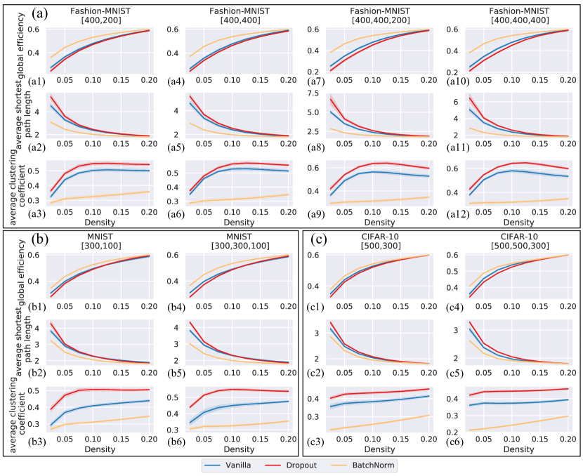
Figure 3: Graph theoretical properties of the functional networks with different densities for the FCNs trained on the (a) Fashion-MNIST, (b) MNIST, and (c) CIFAR-10 datasets. The blue, red, and orange curves represent the corresponding average index with the error bars of the functional networks on the first, second, and third groups, respectively.

For each group of the trained FCNs, we constructed and analyzed their functional networks using GTA. First, an appropriate density for the functional network construction should be selected. A high density introduces too much noise, whereas a low density makes important connectivities removed. As a result, for FCN, we constructed the functional network sequence by setting the density ranging from 2.5% to 20% with a 2.5% increment. Then, we characterized the FCNs by the global efficiency, average shortest path length, and average clustering coefficient of their functional networks. Specifically, the clustering coefficient of a node measures the proportion of edges between its neighborhood, divided by the maximum possible number of edges. In complex brain network analysis, the former two measure functional integration and information transmission of the network. The latter assesses the topological redundancy, local fault tolerance, and functional specialization (Fornito et al., 2016).

As shown in Figure 3, the standard deviations of the graph theoretical properties are small for the FCNs in the same group, which suggests that the graph theoretical properties are stable to the initial values. Moreover, at the same density, the global efficiency of the BatchNorm group is over that of the vanilla group, whereas that of the dropout group is below it. Meanwhile, for the average shortest path length and average clustering coefficient, the corresponding relation of quantity between them is opposite: the values of the dropout group are larger than those of the vanilla group, and those of the BatchNorm group are less. The graph theoretical differences between the functional networks in various groups show that the regularization techniques have different impacts on FCNs. The models with batch normalization have higher global information transmission capability and more rapid, integrated, and efficient communication between neurons, which improves network performance. However, the improvement of efficiency comes at the cost of a decrease in the clustering coefficient. The clustering coefficient measures the network fault tolerance, and a highly clustered network is resilient to random attacks (Fornito et al., 2016). The decrease in the fault tolerance leads to a decline in adversarial robustness.

In contrast to batch normalization, dropout raises the average clustering coefficient and average shortest path length while lowering the global efficiency. The high average clustering coefficient demonstrates that numerous small subgraphs with tight internal integration exist in the functional network. Moreover, the neurons in a subgraph encode comparable features, which can be considered a functional group. The functional groups facilitate functional specialization within the network, which contributes to fast and efficient information processing (Ringo et al., 1994), and increase the network redundancy and fault tolerance. Therefore, the robustness and model performance are improved.

In conclusion, batch normalization and dropout have different mechanisms: (1) Batch normalization enhances model performance by increasing the global efficiency of neural networks but reduces adversarial robustness by lowering the fault tolerance. (2) Dropout facilitates functional specialization and fault tolerance by increasing functional groups, which improves the generalization ability and robustness of neural networks. According to this conclusion, we can explain the decline in network performance when dropout and batch normalization are combined practically.

5.3.2 TDA and Clustering Experiments

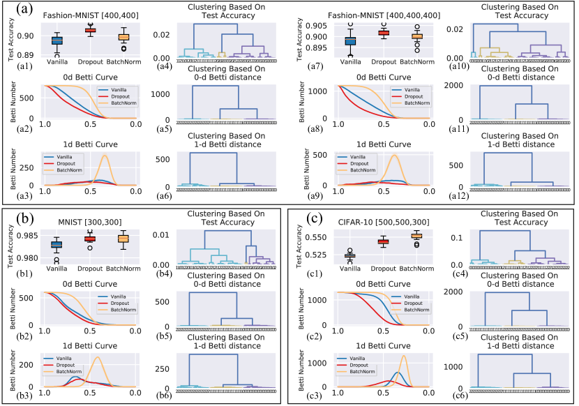
Figure 4: Direct outcome of TDA for the FCNs trained on the (a) Fashion-MNIST, (b) MNIST, and (c) CIFAR-10 datasets: a1, a7, b1, and c1: the box plots of the test accuracies for the FCNs; a2, a3, a8, a9, b2, b3, c2, and c3: the average zero- and one-dimensional Betti curves with the error bars of the functional networks; a4-a6, a10-a11, b4-b6, and c4-c6: the dendrograms of hierarchical clustering by test accuracies, and zero- and one-dimensional Betti distances, where 0, 1, and 2 denote the FCNs in the vanilla, dropout, and BatchNorm groups, respectively.

Compared with GTA, TDA depicts the higher-dimensional interactions at different resolutions without the density selection in GTA and is more robust to noise. In TDA, a network is modeled as a simplicial complex $K$, which is a set of simplexes $\tau$. A $k$-simplex $\tau_{i}$ is the convex hull of $k+1$ vertices, denoted as $\tau_{i}=[v_{i0},v_{i1},\cdots,v_{ik}]$. A face of $\tau_{i}$ is the convex hull of its vertice subset.

Previous studies (Rieck et al., 2019; Watanabe and Yamana, 2021) showed that the complexity of FCNs could be measured by their zero- and one-dimensional structural topological features. Meanwhile, TDA is also used to capture the topological differences between functional brain networks to identify and classify various types of brains (Billings et al., 2021). In this work, we applied TDA to obtain the zero- and one-dimensional Betti number curve of the functional network to explain the mechanisms of dropout and batch normalization. To show that TDA characterizes deep neural networks, the clustering experiments were performed to distinguish the FCNs trained with different regularizations according to their functional topological features.

First, we modeled a functional network as a weighted simplicial complex $K$. Given a weighted graph $F(V,E_{f},W_{f})$ with the weight function $\psi$, we can define a simplicial complex $K=\{[v_{i0},v_{i1},...,v_{ik}]|v_{i0},v_{i1},...,v_{ik}\in V{\ and\ }0\leq k<n\}$ with a weight function $\phi:K\to\mathbb{R}$, i.e.,

$$\phi(\tau_{i})=\begin{cases}1,&\text{if }\tau_{i}=[v_{i0}],\\ \psi((v_{i0},v_{i1})),&\text{if }\tau_{i}=[v_{i0},v_{i1}],\\ \mathop{\min}_{\kappa\subset\tau_{i}}\phi(\kappa),&otherwise,\end{cases}$$ (11)

where $\psi((v_{i0},v_{i1}))$ is the weight of the edge $(v_{i0},v_{i1})$ in $F$, and $\kappa$ represents any face of the simplex $\tau_{i}$. Then, the super-level filtration was adapted to get the $k$-dimensional Betti number curve $\beta_{k}(\varepsilon)$ of $K$, where $\varepsilon$ represents the filtration threshold (Dong et al., 2021).

For $F(V,E_{f},W_{f})$, the nodes in $V$ are modeled as 0-simplexes with the weights of 1 in $K$. The functional connectivities in $E_{f}$ are modeled as $1$-simplexes with the weights of corresponding functional connectivity strength. Moreover, the $k$-cliques ($k\geq 2$) in $F(V,E_{f},W_{f})$ are modeled as k-simplexes with weights equal to the minimum weight of their faces.

We analyzed the FCNs with architectures [400, 400] and [400, 400, 400] trained on the Fashion-MNIST dataset, the FCNs with [300, 300] trained on the MNIST dataset, and the FCNs with [500, 500, 300] trained on the CIFAR-10 dataset. For the FCN $\mathbb{M}_{i}$, we constructed the corresponding weighted simplicial complex $K^{i}$ and obtained the zero- and one-dimensional Betti number curves $\beta_{0}^{i}(\epsilon)$ and $\beta_{1}^{i}(\epsilon)$ by filtering $K^{i}$ from 1 to 0. The Betti numbers $\beta_{0}^{i}$ and $\beta_{1}^{i}$ represent the numbers of connected components and loops contained in $K^{i}$, respectively. Moreover, the zero- and one-dimensional Betti distances between functional networks were calculated as follows to measure the functional topological differences between the FCNs:

$$d_{k}(K^{i},K^{j})=\int_{\varepsilon}|\beta_{k}^{i}(x)-\beta_{k}^{j}(x)|^{2}dx.$$ (12)

where $k=0,1$. Finally, we clustered the networks hierarchically according to their test accuracies, and zero- and one-dimensional Betti distances. We illustrated the clustering results in the dendrograms.

Figure 4 (a1, a7, b1, and c1) shows that the median test accuracies of the FCNs with regularization are higher than those of the vanilla FCNs. Figure 4 (a2, a3, a8, a9, b2, b3, c2, and c3) displays the average zero- and one-dimensional Betti curves. The small standard deviations of the Betti curves imply that the Betti numbers of functional networks are stable to the initial values.

For the simplicial complexes at the same threshold value $\epsilon$, average $\beta_{0}$ in the BatchNorm group is the largest, followed by that in the vanilla and dropout groups, whereas average $\beta_{0}$ in the dropout group is the smallest. This result indicates that the functional networks in the dropout group have the least number of connected components at the same threshold. That is, the FCNs with dropout possess several functional groups, in which the neurons encode similar features and thus have strong functional connectivities. Therefore, the connected components in the same functional group merge early, causing a small $\beta_{0}$. On the contrary, the FCNs with batch normalization have few and weak functional groups, leading to a large $\beta_{0}$.

Compared with the peak of one-dimensional Betti curves for the vanilla group, that for the BatchNorm group is significantly higher, whereas the peak for the dropout group is lower. The maximum $\beta_{1}$ represents the maximum number of loops that occur in the filtration of the simplicial complex. The combinational effects of numerous neurons in deep neural networks can be revealed through one-dimensional topological features (Watanabe and Yamana, 2021). The loops might attribute to the feature coding in deep neural networks. The previous study (Benz et al., 2021) showed that batch normalization allows the utilization of more useful features to increase accuracy. The highest peak of the one-dimensional Betti curves in the BatchNorm group may suggest that batch normalization potentially improves the coding capability of neural networks by increasing the number of functional loops. Furthermore, $\beta_{0}$ and the maximum $\beta_{1}$ of the functional networks in the dropout and BatchNorm groups change in the opposite tendency. This result implies that dropout and batch normalization have opposing impacts on zero- and one-dimensional topological features, which is in accordance with the observation in GTA.

As shown in Figure 4 (a4-a6, a10-a12, b4-b6, and c4-c6), the FCNs with various regularizations can be correctly clustered according to the zero- and one-dimensional Betti distances while being incorrectly clustered simply using the test accuracies. Although regularization methods enhance network performance, the improvements in test accuracies are insufficient to distinguish regularization techniques. This finding indicates that, compared with test accuracies, TDA indexes can better evaluate and distinguish deep neural networks.

Moreover, the best clustering index is the zero-dimensional Betti distance because it produces a large distance between clusters and a small distance within a cluster. Although the FCNs can be correctly clustered according to the one-dimensional Betti distances, the distances between the vanilla and dropout groups are comparatively small. This finding reflects that batch normalization has a greater impact on the one-dimensional topological structures of the functional network than dropout. The findings also suggest the potential of the functional network and TDA for extracting functional topological features to explain, evaluate, and distinguish deep neural networks.

6 Conclusion

In this work, we propose the functional network as a novel framework for interpretability of deep neural networks. We show that the functional network of FCNs is a small-world network, similar to the brain functional network, suggesting that the two have a similar functional organization. Batch normalization enhances model performance by increasing the global efficiency and the number of functional loops but reduces adversarial robustness by lowering the fault tolerance. Dropout enhances the functional specialization and fault tolerance in models by increasing the number of functional groups and network redundancy, improving the generalization ability and robustness of neural networks. Additionally, the models with different regularizations were clustered correctly according to their functional topological differences, reflecting that topological features based on TDA characterize the FCNs.

In this work, Pearson correlation is used as the measure of statistical dependency between neural activities of neurons. In future work, we will choose other methods to measure functional connectivity. Another interesting avenue is to study the similarities and differences of coding mechanisms between the brain and the deep neural network from the perspective of the functional network, which will promote the research of brain-inspired intelligence.

References

- Akula et al. (2020) A. R. Akula, S. Wang, and S. Zhu. Cocox: Generating conceptual and counterfactual explanations via fault-lines. In The Thirty-Fourth AAAI Conference on Artificial Intelligence, AAAI 2020, The Thirty-Second Innovative Applications of Artificial Intelligence Conference, IAAI 2020, The Tenth AAAI Symposium on Educational Advances in Artificial Intelligence, EAAI 2020, New York, NY, USA, February 7-12, 2020, pages 2594–2601. AAAI Press, 2020. URL https://aaai.org/ojs/index.php/AAAI/article/view/5643.
- Balakrishnan and Ranganathan (2012) R. Balakrishnan and K. Ranganathan. A Textbook of Graph Theory. Springer New York, New York, NY, 2012. ISBN 978-1-4614-4529-6. doi: 10.1007/978-1-4614-4529-6. URL https://doi.org/10.1007/978-1-4614-4529-6.
- Bassett et al. (2011) D. S. Bassett, N. F. Wymbs, M. A. Porter, P. J. Mucha, J. M. Carlson, and S. T. Grafton. Dynamic reconfiguration of human brain networks during learning. Proceedings of the National Academy of Sciences, 108(18):7641–7646, 2011. ISSN 0027-8424. doi: 10.1073/pnas.1018985108. URL https://www.pnas.org/content/108/18/7641.
- Bassett et al. (2015) D. S. Bassett, M. Yang, N. F. Wymbs, and S. T. Grafton. Learning-induced autonomy of sensorimotor systems. Nature Neuroscience, 18(5):744–751, 2015. doi: 10.1038/nn.3993.
- Bau et al. (2017) D. Bau, B. Zhou, A. Khosla, A. Oliva, and A. Torralba. Network dissection: Quantifying interpretability of deep visual representations. In 2017 IEEE Conference on Computer Vision and Pattern Recognition (CVPR), pages 3319–3327, 2017. doi: 10.1109/CVPR.2017.354.
- Beaty et al. (2018) R. E. Beaty, Y. N. Kenett, A. P. Christensen, M. D. Rosenberg, M. Benedek, Q. Chen, A. Fink, J. Qiu, T. R. Kwapil, M. J. Kane, and P. J. Silvia. Robust prediction of individual creative ability from brain functional connectivity. Proceedings of the National Academy of Sciences, 115(5):1087–1092, 2018. ISSN 0027-8424. doi: 10.1073/pnas.1713532115. URL https://www.pnas.org/content/115/5/1087.
- Benz et al. (2021) P. Benz, C. Zhang, and I. S. Kweon. Batch normalization increases adversarial vulnerability and decreases adversarial transferability: A non-robust feature perspective. In Proceedings of the IEEE/CVF International Conference on Computer Vision (ICCV), pages 7818–7827, October 2021.
- Bi and Zhou (2020) Z. Bi and C. Zhou. Understanding the computation of time using neural network models. Proceedings of the National Academy of Sciences, 117(19):10530–10540, 2020. ISSN 0027-8424. doi: 10.1073/pnas.1921609117. URL https://www.pnas.org/content/117/19/10530.
- Bien and Tibshirani (2011) J. Bien and R. Tibshirani. Prototype selection for interpretable classification. The Annals of Applied Statistics, 5(4):2403 – 2424, 2011. doi: 10.1214/11-AOAS495. URL https://doi.org/10.1214/11-AOAS495.
- Billings et al. (2021) J. Billings, M. Saggar, J. Hlinka, S. Keilholz, and G. Petri. Simplicial and topological descriptions of human brain dynamics. Network Neuroscience, 5(2):549–568, 06 2021. ISSN 2472-1751. doi: 10.1162/netn˙a˙00190. URL https://doi.org/10.1162/netn_a_00190.
- Boz (2002) O. Boz. Extracting decision trees from trained neural networks. KDD ’02, page 456–461, New York, NY, USA, 2002. Association for Computing Machinery. ISBN 158113567X. doi: 10.1145/775047.775113. URL https://doi.org/10.1145/775047.775113.
- Cadieu et al. (2014) C. F. Cadieu, H. Hong, D. Yamins, N. Pinto, D. Ardila, E. A. Solomon, N. J. Majaj, J. J. Dicarlo, and M. Bethge. Deep neural networks rival the representation of primate it cortex for core visual object recognition. Plos Computational Biology, 10(12):e1003963, 2014. doi: 10.1371/journal.pcbi.1003963.
- Dabaghian et al. (2012) Y. Dabaghian, F. Mémoli, L. Frank, and G. Carlsson. A topological paradigm for hippocampal spatial map formation using persistent homology. PLoS computational biology, 8(8):e1002581, 2012. ISSN 1553-734X. doi: 10.1371/journal.pcbi.1002581. URL https://europepmc.org/articles/PMC3415417.
- Dalvi et al. (2019) F. Dalvi, N. Durrani, H. Sajjad, Y. Belinkov, A. Bau, and J. Glass. What is one grain of sand in the desert? analyzing individual neurons in deep nlp models. Proceedings of the AAAI Conference on Artificial Intelligence, 33(01):6309–6317, Jul. 2019. doi: 10.1609/aaai.v33i01.33016309. URL https://ojs.aaai.org/index.php/AAAI/article/view/4592.
- Daub et al. (2004) C. O. Daub, R. Steuer, J. Selbig, and S. Kloska. Estimating mutual information using b-spline functions–an improved similarity measure for analysing gene expression data. BMC bioinformatics, 5:118, August 2004. ISSN 1471-2105. doi: 10.1186/1471-2105-5-118. URL https://europepmc.org/articles/PMC516800.
- Deng (2012) L. Deng. The mnist database of handwritten digit images for machine learning research. IEEE Signal Processing Magazine, 29(6):141–142, 2012.
- Dodel et al. (2002) S. Dodel, J. Herrmann, and T. Geisel. Functional connectivity by cross-correlation clustering. Neurocomputing, 44-46:1065–1070, 2002. ISSN 0925-2312. doi: https://doi.org/10.1016/S0925-2312(02)00416-2. URL https://www.sciencedirect.com/science/article/pii/S0925231202004162. Computational Neuroscience Trends in Research 2002.
- Dong et al. (2021) Z. Dong, J. Pu, and H. Lin. Multiscale persistent topological descriptor for porous structure retrieval. Computer Aided Geometric Design, 88:102004, 2021. ISSN 0167-8396. doi: https://doi.org/10.1016/j.cagd.2021.102004. URL https://www.sciencedirect.com/science/article/pii/S0167839621000492.
- Edelsbrunner and Harer (2009) H. Edelsbrunner and J. Harer. Computational Topology: An Introduction. American Mathematical Society, 2009.
- Eguíluz et al. (2005) V. M. Eguíluz, D. R. Chialvo, G. A. Cecchi, M. Baliki, and A. V. Apkarian. Scale-free brain functional networks. Phys. Rev. Lett., 94:018102, Jan 2005. doi: 10.1103/PhysRevLett.94.018102. URL https://link.aps.org/doi/10.1103/PhysRevLett.94.018102.
- El Mhamdi et al. (2017) E. M. El Mhamdi, R. Guerraoui, and S. Rouault. On the robustness of a neural network. In 2017 IEEE 36th Symposium on Reliable Distributed Systems (SRDS), pages 84–93, 2017. doi: 10.1109/SRDS.2017.21.
- Fornito et al. (2016) A. Fornito, A. Zalesky, and E. T. Bullmore. Fundamentals of Brain Network Analysis. Academic Press, San Diego, 2016. ISBN 978-0-12-407908-3. doi: 10.1016/C2012-0-06036-X. URL https://www.sciencedirect.com/book/9780124079083.
- Güçlü and van Gerven (2015) U. Güçlü and M. A. J. van Gerven. Deep neural networks reveal a gradient in the complexity of neural representations across the ventral stream. Journal of Neuroscience, 35(27):10005 – 10014, 2015. ISSN 02706474. doi: 10.1523/JNEUROSCI.5023-14.2015. URL https://www.jneurosci.org/content/35/27/10005.
- Heumann et al. (2016) C. Heumann, M. Schomaker, and Shalabh. Association of Two Variables, pages 67–94. Springer International Publishing, Cham, 2016. ISBN 978-3-319-46162-5. doi: 10.1007/978-3-319-46162-5˙4. URL https://doi.org/10.1007/978-3-319-46162-5_4.
- Humphries and Gurney (2008) M. D. Humphries and K. Gurney. Network ’small-world-ness’: a quantitative method for determining canonical network equivalence. PLoS ONE, 3(4), 2008. doi: 10.1371/journal.pone.0002051.
- Ioffe and Szegedy (2015) S. Ioffe and C. Szegedy. Batch normalization: Accelerating deep network training by reducing internal covariate shift. In F. Bach and D. Blei, editors, Proceedings of the 32nd International Conference on Machine Learning, volume 37 of Proceedings of Machine Learning Research, pages 448–456, Lille, France, 07–09 Jul 2015. PMLR. URL https://proceedings.mlr.press/v37/ioffe15.html.
- Kim et al. (2014) B. Kim, C. Rudin, and J. Shah. The bayesian case model: A generative approach for case-based reasoning and prototype classification. In Proceedings of the 27th International Conference on Neural Information Processing Systems - Volume 2, NIPS’14, page 1952–1960, Cambridge, MA, USA, 2014. MIT Press.
- Krizhevsky (2009) A. Krizhevsky. Learning multiple layers of features from tiny images. Technical report, 2009.
- Li et al. (2019) X. Li, S. Chen, X. Hu, and J. Yang. Understanding the disharmony between dropout and batch normalization by variance shift. In 2019 IEEE/CVF Conference on Computer Vision and Pattern Recognition (CVPR), pages 2677–2685, 2019. doi: 10.1109/CVPR.2019.00279.
- Lv et al. (2013) J. Lv, X. Li, D. Zhu, X. Jiang, X. Zhang, X. Hu, T. Zhang, L. Guo, and T. Liu. Sparse representation of group-wise fmri signals. In K. Mori, I. Sakuma, Y. Sato, C. Barillot, and N. Navab, editors, Medical Image Computing and Computer-Assisted Intervention – MICCAI 2013, pages 608–616, Berlin, Heidelberg, 2013. Springer Berlin Heidelberg. ISBN 978-3-642-40760-4.
- McNabb et al. (2018) C. B. McNabb, R. J. Tait, M. E. McIlwain, V. M. Anderson, J. Suckling, R. R. Kydd, and B. R. Russell. Functional network dysconnectivity as a biomarker of treatment resistance in schizophrenia. Schizophrenia Research, 195:160–167, 2018. ISSN 0920-9964. doi: https://doi.org/10.1016/j.schres.2017.10.015. URL https://www.sciencedirect.com/science/article/pii/S0920996417306242.
- Menon (2013) V. Menon. Developmental pathways to functional brain networks: emerging principles. Trends in Cognitive Sciences, 17(12):627–640, 2013. doi: 10.1016/j.tics.2013.09.015.
- Moradi et al. (2020) R. Moradi, R. Berangi, and B. Minaei. A survey of regularization strategies for deep models. Artificial Intelligence Review, 53(6):3947–3986, 2020. doi: 10.1007/s10462-019-09784-7.
- Naitzat et al. (2020) G. Naitzat, A. Zhitnikov, and L.-H. Lim. Topology of deep neural networks. Journal of Machine Learning Research, 21(184):1–40, 2020. URL http://jmlr.org/papers/v21/20-345.html.
- Nayak (2009) R. Nayak. Generating rules with predicates, terms and variables from the pruned neural networks. Neural Networks, 22(4):405–414, 2009. ISSN 0893-6080. doi: https://doi.org/10.1016/j.neunet.2009.02.001. URL https://www.sciencedirect.com/science/article/pii/S0893608009000161.
- Park and Kwak (2017) S. Park and N. Kwak. Analysis on the dropout effect in convolutional neural networks. In S.-H. Lai, V. Lepetit, K. Nishino, and Y. Sato, editors, Computer Vision – ACCV 2016, pages 189–204, Cham, 2017. Springer International Publishing. ISBN 978-3-319-54184-6.
- Petri et al. (2014) G. Petri, P. Expert, F. Turkheimer, R. Carhart-Harris, D. Nutt, P. J. Hellyer, and F. Vaccarino. Homological scaffolds of brain functional networks. Journal of The Royal Society Interface, 11(101):20140873, 2014. doi: 10.1098/rsif.2014.0873. URL https://royalsocietypublishing.org/doi/abs/10.1098/rsif.2014.0873.
- Raghu et al. (2017) M. Raghu, B. Poole, J. Kleinberg, S. Ganguli, and J. Sohl-Dickstein. On the expressive power of deep neural networks. In D. Precup and Y. W. Teh, editors, Proceedings of the 34th International Conference on Machine Learning, volume 70 of Proceedings of Machine Learning Research, pages 2847–2854. PMLR, 06–11 Aug 2017. URL https://proceedings.mlr.press/v70/raghu17a.html.
- Ribeiro et al. (2016) M. T. Ribeiro, S. Singh, and C. Guestrin. ”why should i trust you?”: Explaining the predictions of any classifier. In the 22nd ACM SIGKDD International Conference, 2016.
- Rieck et al. (2019) B. Rieck, M. Togninalli, C. Bock, M. Moor, M. Horn, T. Gumbsch, and K. Borgwardt. Neural persistence: A complexity measure for deep neural networks using algebraic topology. In 7th International Conference on Learning Representations, ICLR 2019, New Orleans, LA, USA, May 6-9, 2019. OpenReview.net, 2019. URL https://openreview.net/forum?id=ByxkijC5FQ.
- Ringo et al. (1994) J. L. Ringo, R. W. Doty, S. Demeter, and P. Y. Simard. Time Is of the Essence: A Conjecture that Hemispheric Specialization Arises from Interhemispheric Conduction Delay. Cerebral Cortex, 4(4):331–343, 07 1994. ISSN 1047-3211. doi: 10.1093/cercor/4.4.331. URL https://doi.org/10.1093/cercor/4.4.331.
- Rudie et al. (2013) J. Rudie, J. Brown, D. Beck-Pancer, L. Hernandez, E. Dennis, P. Thompson, S. Bookheimer, and M. Dapretto. Altered functional and structural brain network organization in autism. NeuroImage: Clinical, 2:79–94, 2013. ISSN 2213-1582. doi: https://doi.org/10.1016/j.nicl.2012.11.006. URL https://www.sciencedirect.com/science/article/pii/S2213158212000356.
- Ryali et al. (2012) S. Ryali, T. Chen, K. Supekar, and V. Menon. Estimation of functional connectivity in fmri data using stability selection-based sparse partial correlation with elastic net penalty. NeuroImage, 59(4):3852–3861, 2012. ISSN 1053-8119. doi: https://doi.org/10.1016/j.neuroimage.2011.11.054. URL https://www.sciencedirect.com/science/article/pii/S105381191101336X.
- Shnier et al. (2019) D. Shnier, M. A. Voineagu, and I. Voineagu. Persistent homology analysis of brain transcriptome data in autism. Journal of the Royal Society, Interface, 16(158), 2019. doi: 10.1098/rsif.2019.0531.
- Singh et al. (2008) G. Singh, F. Memoli, T. Ishkhanov, G. Sapiro, G. Carlsson, and D. L. Ringach. Topological analysis of population activity in visual cortex. Journal of Vision, 8(8):11–11, 06 2008. ISSN 1534-7362. doi: 10.1167/8.8.11. URL https://doi.org/10.1167/8.8.11.
- Srivastava et al. (2014) N. Srivastava, G. Hinton, A. Krizhevsky, I. Sutskever, and R. Salakhutdinov. Dropout: A simple way to prevent neural networks from overfitting. Journal of Machine Learning Research, 15(1):1929–1958, 2014.
- Stam (2004) C. Stam. Functional connectivity patterns of human magnetoencephalographic recordings: a ‘small-world’ network? Neuroscience Letters, 355(1):25–28, 2004. ISSN 0304-3940. doi: https://doi.org/10.1016/j.neulet.2003.10.063. URL https://www.sciencedirect.com/science/article/pii/S0304394003012722.
- Strogatz (2001) S. H. Strogatz. Exploring complex networks. Nature, 410(6825):268–276, mar 2001. doi: 10.1038/35065725.
- Štrumbelj et al. (2009) E. Štrumbelj, I. Kononenko, and M. Robnik Šikonja. Explaining instance classifications with interactions of subsets of feature values. Data & Knowledge Engineering, 68(10):886–904, 2009. ISSN 0169-023X. doi: https://doi.org/10.1016/j.datak.2009.01.004. URL https://www.sciencedirect.com/science/article/pii/S0169023X09000056.
- Varoquaux et al. (2013) G. Varoquaux, Y. Schwartz, P. Pinel, and B. Thirion. Cohort-level brain mapping: Learning cognitive atoms to single out specialized regions. In J. C. Gee, S. Joshi, K. M. Pohl, W. M. Wells, and L. Zöllei, editors, Information Processing in Medical Imaging, pages 438–449, Berlin, Heidelberg, 2013. Springer Berlin Heidelberg. ISBN 978-3-642-38868-2.
- Watanabe and Yamana (2021) S. Watanabe and H. Yamana. Topological measurement of deep neural networks using persistent homology. Annals of Mathematics and Artificial Intelligence, 2021. doi: 10.1007/s10472-021-09761-3.
- Xiao et al. (2017) H. Xiao, K. Rasul, and R. Vollgraf. Fashion-mnist: a novel image dataset for benchmarking machine learning algorithms, 2017.
- Yamins et al. (2014) D. L. K. Yamins, H. Hong, C. F. Cadieu, E. A. Solomon, D. Seibert, and J. J. DiCarlo. Performance-optimized hierarchical models predict neural responses in higher visual cortex. Proceedings of the National Academy of Sciences, 111(23):8619–8624, 2014. doi: 10.1073/pnas.1403112111. URL https://www.pnas.org/content/early/2014/05/08/1403112111.
- Yang et al. (2019) G. R. Yang, M. R. Joglekar, H. F. Song, W. T. Newsome, and X.-J. Wang. Task representations in neural networks trained to perform many cognitive tasks. Nature Neuroscience, 22(2):297–306, 2019. ISSN 1546-1726. doi: 10.1038/s41593-018-0310-2.
- Young et al. (2000) M. P. Young, K. E. Stephan, C. Hilgetag, G. A. P. C. Burns, M. A. O’Neill, M. P. Young, and R. Kotter. Computational analysis of functional connectivity between areas of primate cerebral cortex. Philosophical Transactions of the Royal Society of London. Series B: Biological Sciences, 355(1393):111–126, 2000. doi: 10.1098/rstb.2000.0552. URL https://royalsocietypublishing.org/doi/abs/10.1098/rstb.2000.0552.
- Zeiler and Fergus (2014) M. D. Zeiler and R. Fergus. Visualizing and understanding convolutional networks. In D. Fleet, T. Pajdla, B. Schiele, and T. Tuytelaars, editors, Computer Vision – ECCV 2014, pages 818–833, Cham, 2014. Springer International Publishing. ISBN 978-3-319-10590-1.
- Zhang et al. (2021) C. Zhang, S. Bengio, M. Hardt, B. Recht, and O. Vinyals. Understanding deep learning (still) requires rethinking generalization. Commun. ACM, 64(3):107–115, Feb. 2021. ISSN 0001-0782. doi: 10.1145/3446776. URL https://doi.org/10.1145/3446776.