Simple Recurrence Improves Masked Language Models

Abstract

In this work, we explore whether modeling recurrence into the Transformer architecture can both be beneficial and efficient, by building an extremely simple recurrent module into the Transformer. We compare our model to baselines following the training and evaluation recipe of BERT. Our results confirm that recurrence can indeed improve Transformer models by a consistent margin, without requiring low-level performance optimizations, and while keeping the number of parameters constant. For example, our base model achieves an absolute improvement of 2.1 points averaged across 10 tasks and also demonstrates increased stability in fine-tuning over a range of learning rates.

1 Introduction

While the Transformer Vaswani et al. (2017) relies solely on attention mechanisms for sequence modeling, many recent works have incorporated recurrence into the architecture and demonstrated superior performance in various applications. For example, such modifications were shown to be beneficial for modeling long-range inputs Hutchins et al. (2022), accelerating language model training Lei (2021) and improving translation and speech recognition systems Hao et al. (2019); Pan et al. (2022); Chen et al. (2018).

Even though combining attention and recurrence is useful in many cases, very little efforts have gone into language model pre-training and fine-tuning. In particular, one open question is whether a combined model can be pre-trained and fine-tuned to achieve stronger accuracy compared to its attention-only counterparts.

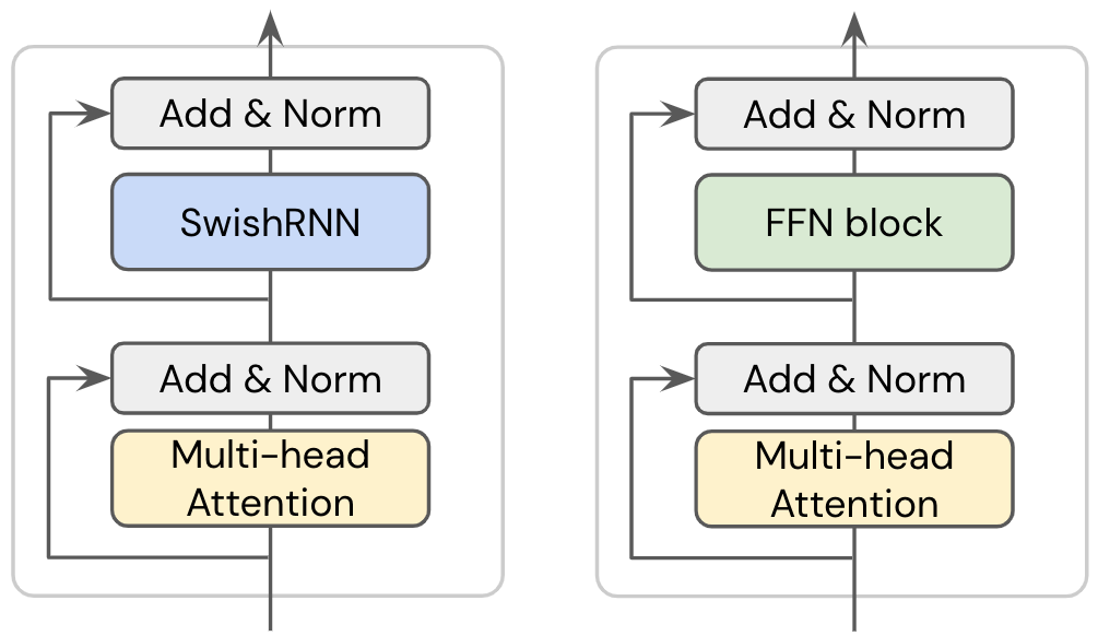
Figure 1: Our model architecture (left) and the original Transformer (right) for masked language modeling. We replace the feed-forward blocks with light-weight recurrence, which is interleaved with attention blocks.

We study this question in the case of masked language model training, specifically BERT Devlin et al. (2019). Unlike previous work Huang et al. (2020), we are interested in retaining the training efficiency of the model when combining attention and recurrence. That is, the amount of parameters and computation should remain comparable to the baseline Transformer model. However, making a recurrent model operating at a similar computation throughput as attention can be challenging, such as requiring CUDA implementations for GPUs Appleyard et al. (2016); Bradbury et al. (2017). To mitigate this issue, we propose a simple recurrent implementation which we call SwishRNN. SwishRNN uses minimal operations in the recurrence step in order to accelerate computation, and can run on both TPUs and GPUs using a few lines of code in machine learning libraries such as Tensorflow. We incorporate SwishRNN into BERT by substituting the feed-forward layers and keeping the same number of model parameters.

We pre-train our model and BERT baselines using the standard Wikipedia+Book corpus, and compare their fine-tuning performance on 10 tasks selected in the GLUE and SuperGLUE benchmark. Our results confirm that modeling recurrence jointly with attention is indeed helpful, resulting in an average improvement of 2.1 points for the BERT-base models and 0.6 points for the large models. The combined model also exhibits better stability, achieving more consistent fine-tuning results over a range of learning rates.

2 Model

In this section, we first give a quick overview of our model architecture and then describe the recurrence module SwishRNN in more details.

2.1 Notation and Background

The Transformer architecture interleaves a multi-headed attention block, $F_{\textrm{att}}$, with feed forward block, $F_{\textrm{ffn}}$, as shown in Figure 1. Between each block is a residual connection and layer normalization that we denote as ${F}_{\textrm{Add+Norm}}$. These functions are defined in the Appendix for completeness.

At each layer $k$, the hidden state of a Transformer is represented by an $l\times d$ matrix ${\bm{X}}^{k}$, where $l$ is the sequence length and $d$ the hidden size. We define the intermediate hidden state $\bar{{\bm{X}}}^{k}$ and input to the next layer ${\bm{X}}^{k+1}$ as:

$$\bar{{\bm{X}}}^{k} :=F_{\textrm{Add+Norm}}\left(F_{\textrm{att}}({\bm{X}}^{k}),{\bm{X}}^{k}\right)$$

$${\bm{X}}^{k+1} :=F_{\textrm{Add+Norm}}\left(F_{\textrm{ffn}}(\bar{{\bm{X}}}^{k}),\bar{{\bm{X}}}^{k}\right)$$ (1)

2.2 Architecture

Compared to the original architecture, we simply replace every feed-forward block $F_{\textrm{ffn}}$ with a recurrence block as shown in Figure 1.

SwishRNN

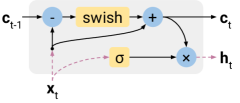
Figure 2: The SwishRNN cell. A red dotted line represents a linear transformation.

Modern accelerator hardwares such as TPUs and GPUs are highly optimized for matrix multiplications, making feed-forward architectures such as attention very efficient. Recurrent networks (RNNs) however involves sequential operations that cannot run in parallel. In order to achieve a training efficiency comparable to the original Transformer, we use minimal sequential operations and demonstrate they are sufficient to improve the modeling power.

Specifically, SwishRNN uses only two matrix multiplications and an extremely simple sequential pooling operation. Let $\bar{{\bm{x}}}[i]:=\bar{{\bm{X}}}[i,:]$ be the intermediate hidden vector of the $i$-th position (from Eq. 1). SwishRNN first computes two linear transformations of $\bar{{\bm{X}}}$:

$$\bar{{\bm{X}}}_{1}=\bar{{\bm{X}}}{\bm{W}}_{1},\quad\bar{{\bm{X}}}_{2}=\bar{{\bm{X}}}{\bm{W}}_{2}$$ (2)

where ${\bm{W}}_{1}$ and ${\bm{W}}_{2}$ are $d\times d^{\prime}$ parameter matrices optimized during training, $d$ is the input and output dimension of the model, and $d^{\prime}$ is the intermediate dimension for recurrence. The hidden vectors $\{{\bm{c}}[i]\}_{i=1}^{l}$ are calculated as follows

$${\bm{c}}[i]=\texttt{Swish}\left({\bm{c}}[i\text{-}1]-\bar{{\bm{x}}}_{1}[i]\right)+\bar{{\bm{x}}}_{1}[i]$$ (3)

where $\texttt{Swish}()$ is the element-wise Swish activation function Ramachandran et al. (2018). We use a $l\times d^{\prime}$ matrix ${\bm{C}}$ to represent the concatenated version of $\{{\bm{c}}[i]\}_{i=1}^{l}$, and set ${\bm{c}}[0]$ as an all-zero vector for simplicity. Intuitively, step (2) can be interpreted as a pooling operator where the greater value between ${\bm{c}}[i\text{-}1]$ and $\bar{{\bm{x}}}_{1}[i]$ are selected.

The output vectors are obtained using a multiplicative gating similar to other RNNs such as LSTM, followed by a linear layer with weights ${\bm{W}}_{3}$:

$$\mathbf{H}={\bm{W}}_{3}\left((\mathbf{C}+{\bm{b}}_{c})\odot\sigma(\mathbf{X}_{2}+{\bm{b}}_{\sigma})\right)+{\bm{b}}_{3}$$ (4)

where $\sigma()$ is a gating activation function. We experimented with sigmoid activation and the GeLU activation (Hendrycks and Gimpel, 2016) used in BERT, and found the latter to achieve lower training loss. Finally, analogous to Eq. 1, we set ${\bm{X}}_{k+1}:=F_{\textrm{Add+Norm}}({\bm{H}},\bar{{\bm{X}}}^{k})$.

Speeding up recurrence

In our experiments, we implement the recurrence step (2) using the scan() function in Tensorflow. Our model using this simple implementation runs 40% slower than the standard Transformer, but is already much faster than other heavier RNNs such as LSTM. For example, a Transformer model combined with LSTM can run multiple times slower Huang et al. (2020).

	BoolQ	CoLA	MNLI	MRPC	MultiRC	QNLI	QQP	RTE	SST2	STSB	Avg
Base model (12 layers, $d=768$)
BERT-orig	73.3%	82.0%	84.8%	88.5%	69.5%	91.0%	87.7%	64.0%	93.7%	84.2%	81.9%
BERT-rab	70.1%	73.7%	85.4%	89.8%	70.3%	92.1%	87.5%	66.4%	91.1%	83.8%	81.0%
Ours	77.9%	80.8%	85.9%	90.4%	74.2%	92.5%	88.2%	70.8%	93.8%	85.7%	84.0%
Large model (24 layers, $d=1024$)
BERT-orig	84.5%	81.4%	89.0%	93.5%	79.6%	94.2%	88.6%	84.0%	95.3%	87.9%	87.8%
BERT-rab	84.5%	75.0%	88.9%	92.2%	80.9%	94.2%	88.4%	78.8%	93.1%	87.2%	86.3%
Ours	86.1%	84.8%	88.9%	92.9%	81.2%	94.3%	88.7%	85.0%	95.3%	87.2%	88.4%
Previously reported results (Large model)
RoBERTa†	-	66.3%	89.0%	90.2%	-	93.9%	91.9%	84.5%	95.3%	91.6%	-
BERT†	-	60.6%	86.6%	88.0%	-	92.3%	91.3%	70.4%	93.2%	90.0%	-
BERT‡	-	61.2%	86.6%	79.5%	-	93.1%	88.4%	68.9%	94.7%	89.6%	-

Table 1: Averaged development set results of all models. We perform 3 independent fine-tuning runs for each model and dataset. For comprehensive study, we also include previously reported results of large BERT models, although training details may differ in this and previous work. Our baseline models are strong compared to previously reported results. ${\dagger}$ indicate results from Liu et al. (2019) and ${\ddagger}$ are results from Wettig et al. (2022) using an efficient training recipe and 40% masking rate.

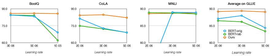
Figure 3: Stability of fine-tuning results given different learning rates. Results are averaged across 3 independent runs for each setting. Our model is more robust to the range of learning rates tested.

We further improve the speed by increasing the step size for the RNN. Specifically, $\mathbf{c}[i]$ is calculated using $\mathbf{c}[i-k]$ and $\mathbf{x}_{1}[i]$ with a step size $k>1$. Each recurrent step can process $k$ consecutive tokens at a time and only $\lceil l/k\rceil$ steps are needed. In our experiments, we interleave the step size $k\in\{1,2,4\}$ across recurrent layers and found this to perform on par with using a fixed step size of 1. Our model with variable step sizes has a marginal 20% - 30% slow-down compared to the standard Transformer model when training on TPUs.

Note that SwishRNN can be made significantly faster using optimized implementation such as CUDA kernel fusion adopted in QRNN and SRU Bradbury et al. (2017); Lei et al. (2018). We leave this for future work as custom kernel fusion is not readily available for TPUs.

3 Experimental Setup

Datasets

Following BERT Devlin et al. (2019), we evaluate all models by pre-training them with the masked language model (MLM) objective and then fine-tuning them on a wide range of downstream tasks. We use the Wikipedia and BookCorpus Zhu et al. (2015) for pre-training, and 10 datasets from the GLUE Wang et al. (2018) and SuperGLUE benchmark Wang et al. (2019) including the BoolQ, CoLa, MNLI, MRPC, MultiRC, QNLI, QQP, RTE, SST2 and STS-B datasets.

Baselines

We compare with two BERT variants. BERT-orig is the original BERT model using the multi-head attention described in Vaswani et al. (2017) and learned absolute positional encoding. The second variant BERT-rab adds the relative attention bias to each attention layer, following the T5 model Raffel et al. (2020). Our model is the same as BERT-rab except we replace every FFN block with SwishRNN. The inner hidden size $d^{\prime}$ of SwishRNN blocks is decreased such that the total number of parameters are similar to the BERT baselines. Following Devlin et al. (2019), we experiment with two model sizes – a base model setting consists of 12 Transformer layers and a large model setting using 24 layers. The detailed model configurations are given in Appendix B.

Step size(s) of RNNs	CoLA	MNLI	MRPC	QNLI	QQP	RTE	SST2	STSB	Time
Base model (12 layers, $d=768$)
$\ 1$	79.4%	85.9%	90.8%	92.1%	88.1%	68.0%	92.7%	86.3%	1.4$\times$
$\ 2$	75.5%	85.9%	88.6%	92.4%	88.1%	64.9%	92.1%	83.1%	1.2$\times$
$\ \{1,2,4\}$	80.8%	85.9%	90.4%	92.5%	88.2%	70.8%	93.8%	85.7%	1.2$\times$
Large model (24 layers, $d=1024$)
$\ 1$	84.7%	89.0%	92.5%	94.5%	88.5%	83.9%	95.6%	87.9%	1.4$\times$
$\ \{1,2,4\}$	84.8%	88.9%	92.9%	94.3%	88.7%	85.0%	95.3%	87.2%	1.3$\times$

Table 2: Fine-tuning results on the GLUE datasets using different step sizes for the recurrent module in our model. We report averaged results and the pre-training time in relative to that of BERT-rab model. Using variable step sizes trains faster and obtains results on par with using step size 1.

Training

Our pre-training recipe is similar to recent work Liu et al. (2019); Izsak et al. (2021); Wettig et al. (2022). Specifically, we do not use the next sentence prediction objective and simply replace 15% input tokens with the special [MASK] token. We also use a larger batch size and fewer training steps following recent work. Specifically, we use a batch size of 1024 for base models and 4096 for large models. The maximum number of pre-training steps is set to 300K.

To reduce the variance, we run 3 independent fine-tuning trials for every model and fine-tuning task, and report the averaged results. We also tune the learning rate separately for each model and fine-tuning task. The training details are provided in Appendix B.

4 Results

Overall results

Table 1 presents the fine-tuning results on 10 datasets. Our base model achieves a substantial improvement, outperforming the BERT-orig and BERT-rab baselines with an average of 2.1 absolute points. The improvement is also consistent, as our base model is better on 9 out of the 10 datasets.

The improvement on large model setting is smaller. Our model obtains an increase of 0.6 point and is better on 6 datasets. We hypothesize that the increased modeling power due to recurrence can be saturating, as making the model much deeper and wider can already enhance the modeling capacity. The gains are still apparent on more challenging datasets such as BoolQ where the input sequences are much longer.

Stability

One interesting observation in our experiments is that combining recurrence and attention improves fine-tuning stability. Figure 3 analyzes model stability by varying the learning rate. We showcase the results on the first 3 datasets (namely BoolQ, CoLA and MNLI) as well as the averaged results on 8 datasets in GLUE. For both BERT model variants, fine-tuning requires more careful tuning of the learning rate. In comparison, our model performs much more consistently across the learning rates tested.

Step size of RNN

Table 2 shows the effect of changing the step size of SwishRNN. Using a step size of 1 is the slowest, since running smaller and more steps adds computational overhead. On the other hand, using a fixed step size of 2 reduces the training cost but hurts the fine-tuning results especially on the CoLA, MRPC, RTE and STS-B datasets. Our best model alternates the step size between 1, 2, and 4 across the recurrent layers, resulting in both faster training and stronger results.

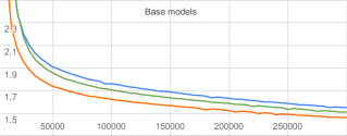
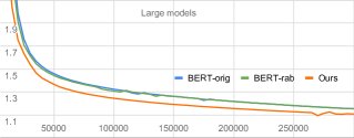
Figure 4: MLM pre-training loss of BERT-orig, BERT-rab and our model architectures.

Pre-training loss

Figure 4 shows the training curves of all models during masked language model training. Our model achieves better loss, indicating increased modeling capacity.

5 Conclusion

In this work, we proposed incorporating an extremely simple recurrent module, SwishRNN, that when incorporated into BERT achieves consistent improvements without requiring low-level performance optimizations. Future directions include extending our work to encoder-decoder pretraining Song et al. (2019) and exploring other domains such as protein modeling Elnaggar et al. (2020).

Appendix A Transformer Architecture

For completeness we review the $F_{\textrm{att}}$, $F_{\textrm{ffn}}$, and ${F}_{\textrm{Add+Norm}}$ blocks used in the Transformer architecture (Figure 1). We omit all bias terms for simplicity.

Attention block ($F_{\textrm{att}}$)

Multi-headed attention with $h$ heads first calculates query ${\bm{Q}}_{m}$, key ${\bm{K}}_{m}$, and value ${\bm{V}}_{m}$ matrices for each head $m\in\{1,..h\}$ by applying linear transformations to the input:

$${\bm{Q}}_{m} ={\bm{X}}{\bm{W}}^{Q}_{m},\;{\bm{K}}_{m}={\bm{X}}{\bm{W}}^{K}_{m},\;{\bm{V}}_{m}={\bm{X}}{\bm{W}}^{V}_{m}$$

Each transformation matrix ${\bm{W}}^{Q}_{m},{\bm{W}}^{K}_{m},{\bm{W}}^{V}_{m}$ is of dimension $d\times d_{h}$ where $d_{h}=d/h$. Attention vectors are then computed for each head, concatenated and multiplied by a linear transformation ${\bm{W}}^{O}$ of dimension $d\times d$:

$${\bm{Z}}_{m} =\mathrm{softmax}\left(\frac{{\bm{Q}}_{m}{\bm{K}}^{\top}_{m}}{\sqrt{d_{h}}}\right){\bm{V}}_{m}$$

$$F_{\textrm{att}}({\bm{X}}) =\textrm{Concat}([{\bm{Z}}_{1},...,{\bm{Z}}_{h}]){\bm{W}}^{O}$$

Feed forward block ($F_{\textrm{ffn}}$)

Following BERT, we use a GeLU nonlinearity (Hendrycks and Gimpel, 2016) i.e. $F_{\textrm{ffn}}({\bm{X}})={\bm{W}}_{f2}(\texttt{GeLU}\left({\bm{W}}_{f1}{\bm{X}})\right)$.

Residual connection and layer normalization ($F_{\textrm{Add+Norm}}$)

. This block applies layer normalization (Ba et al., 2016) to the addition of the two inputs: $F_{\textrm{Add+Norm}}(\tilde{{\bm{X}}},{\bm{X}})=\textrm{LayerNorm}(\tilde{{\bm{X}}}+{\bm{X}})$.

Appendix B Training details

Pre-training

The detailed hyper-parameter configuration for BERT training is shown in Table 3. The training recipe is based on previous works such as RoBERTa Liu et al. (2019) and the 24-hour BERT Izsak et al. (2021). Specifically, compared to the original BERT training recipe which uses 1M training steps and a batch size of 256, the new recipe increases the batch size. The models are trained with much fewer steps and a larger learning rate as a result, which reduces the overall training time. We train base models using 16 TPU v4 chips and large models using 256 chips. For fine-tuning we use only 1 or 2 TPU v4 chips respectively.

	Base model	Large model
Number of layers	12	24
Hidden size	768	1024
Inner hidden size – FFN	3072	4096
Inner hidden size – SwishRNN	2048	2752
Attention heads	12	16
Attention head size	64	64
Dropout	0.1	0.1
Attention dropout	0.1	0.1
Learning rate	0.0003	0.0002
Learning rate warmup steps	20,000	20,000
Learning rate decay	Linear	Linear
Adam $\beta_{1}$	0.9	0.9
Adam $\beta_{2}$	0.98	0.98
Weight decay	0.01	0.01
Batch size	1024	4096
Sequence length	512	512
Training steps	300,000	300,000

Table 3: Hyper-parameters for pre-training the base models and large models in our experiments.

Fine-tuning

We use a batch size of 32 for fine-tuning and evaluate the model performance every 1000 steps. We use Adam optimizer without weight decay during fine-tuning. We use a fixed learning rate tuned among $\{\text{1e-5},\text{5e-6},\text{3e-6},\text{2e-6}\}$ and warm up the learning rate for 1000 steps. The maximum number of training steps of each dataset is presented in Table 4. We set the number proportionally to the size of the dataset and do not tune it in our experiments.

BoolQ	CoLA	MNLI	MRPC	MultiRC	QNLI	QQP	RTE	SST2	STSB
50K	50K	200K	20K	50K	100K	150K	20K	80K	30K

Table 4: Maximum number of fine-tuning step used for each dataset in our experiments.

References

- Appleyard et al. (2016) Jeremy Appleyard, Tomas Kocisky, and Phil Blunsom. 2016. Optimizing performance of recurrent neural networks on gpus.
- Ba et al. (2016) Jimmy Lei Ba, Jamie Ryan Kiros, and Geoffrey E. Hinton. 2016. Layer normalization.
- Bradbury et al. (2017) James Bradbury, Stephen Merity, Caiming Xiong, and Richard Socher. 2017. Quasi-Recurrent Neural Networks. International Conference on Learning Representations (ICLR 2017).
- Chen et al. (2018) Mia Xu Chen, Orhan Firat, Ankur Bapna, Melvin Johnson, Wolfgang Macherey, George F. Foster, Llion Jones, Niki Parmar, Mike Schuster, Zhifeng Chen, Yonghui Wu, and Macduff Hughes. 2018. The best of both worlds: Combining recent advances in neural machine translation. In Proceedings of the 56th Annual Meeting of the Association for Computational Linguistics (ACL).
- Devlin et al. (2019) Jacob Devlin, Ming-Wei Chang, Kenton Lee, and Kristina Toutanova. 2019. BERT: Pre-training of deep bidirectional transformers for language understanding. In Proceedings of the 2019 Conference of the North American Chapter of the Association for Computational Linguistics: Human Language Technologies. Association for Computational Linguistics.
- Elnaggar et al. (2020) Ahmed Elnaggar, Michael Heinzinger, Christian Dallago, Ghalia Rehawi, Yu Wang, Llion Jones, Tom Gibbs, Tamas B. Fehér, Christoph Angerer, Martin Steinegger, Debsindhu Bhowmik, and Burkhard Rost. 2020. Prottrans: Towards cracking the language of life’s code through self-supervised deep learning and high performance computing. bioRxiv.
- Hao et al. (2019) Jie Hao, Xing Wang, Baosong Yang, Longyue Wang, Jinfeng Zhang, and Zhaopeng Tu. 2019. Modeling recurrence for transformer. In Proceedings of the 2019 Conference of the North American Chapter of the Association for Computational Linguistics: Human Language Technologies. Association for Computational Linguistics.
- Hendrycks and Gimpel (2016) Dan Hendrycks and Kevin Gimpel. 2016. Gaussian error linear units (gelus).
- Huang et al. (2020) Zhiheng Huang, Peng Xu, Davis Liang, Ajay Mishra, and Bing Xiang. 2020. Trans-blstm: Transformer with bidirectional lstm for language understanding.
- Hutchins et al. (2022) DeLesley Hutchins, Imanol Schlag, Yuhuai Wu, Ethan Dyer, and Behnam Neyshabur. 2022. Block-recurrent transformers.
- Izsak et al. (2021) Peter Izsak, Moshe Berchansky, and Omer Levy. 2021. How to train BERT with an academic budget. In Proceedings of the 2021 Conference on Empirical Methods in Natural Language Processing.
- Lei (2021) Tao Lei. 2021. When attention meets fast recurrence: Training language models with reduced compute. In Proceedings of the 2021 Conference on Empirical Methods in Natural Language Processing. Association for Computational Linguistics.
- Lei et al. (2018) Tao Lei, Yu Zhang, Sida I. Wang, Hui Dai, and Yoav Artzi. 2018. Simple recurrent units for highly parallelizable recurrence. In Empirical Methods in Natural Language Processing (EMNLP).
- Liu et al. (2019) Yinhan Liu, Myle Ott, Naman Goyal, Jingfei Du, Mandar Joshi, Danqi Chen, Omer Levy, Mike Lewis, Luke Zettlemoyer, and Veselin Stoyanov. 2019. Roberta: A robustly optimized bert pretraining approach.
- Pan et al. (2022) Jing Pan, Tao Lei, Kwangyoun Kim, Kyu J. Han, and Shinji Watanabe. 2022. Sru++: Pioneering fast recurrence with attention for speech recognition. In International Conference on Acoustics, Speech and Signal Processing (ICASSP).
- Raffel et al. (2020) Colin Raffel, Noam Shazeer, Adam Roberts, Katherine Lee, Sharan Narang, Michael Matena, Yanqi Zhou, Wei Li, and Peter J. Liu. 2020. Exploring the limits of transfer learning with a unified text-to-text transformer. Journal of Machine Learning Research, 21(140):1–67.
- Ramachandran et al. (2018) Prajit Ramachandran, Barret Zoph, and Quoc V. Le. 2018. Searching for activation functions.
- Song et al. (2019) Kaitao Song, Xu Tan, Tao Qin, Jianfeng Lu, and Tie-Yan Liu. 2019. Mass: Masked sequence to sequence pre-training for language generation. In ICML.
- Vaswani et al. (2017) Ashish Vaswani, Noam Shazeer, Niki Parmar, Jakob Uszkoreit, Llion Jones, Aidan N Gomez, Ł ukasz Kaiser, and Illia Polosukhin. 2017. Attention is all you need. In Advances in Neural Information Processing Systems, volume 30.
- Wang et al. (2019) Alex Wang, Yada Pruksachatkun, Nikita Nangia, Amanpreet Singh, Julian Michael, Felix Hill, Omer Levy, and Samuel Bowman. 2019. Superglue: A stickier benchmark for general-purpose language understanding systems. In Advances in Neural Information Processing Systems.
- Wang et al. (2018) Alex Wang, Amanpreet Singh, Julian Michael, Felix Hill, Omer Levy, and Samuel Bowman. 2018. GLUE: A multi-task benchmark and analysis platform for natural language understanding. In Proceedings of the 2018 EMNLP Workshop BlackboxNLP: Analyzing and Interpreting Neural Networks for NLP.
- Wettig et al. (2022) Alexander Wettig, Tianyu Gao, Zexuan Zhong, and Danqi Chen. 2022. Should you mask 15masked language modeling?
- Zhu et al. (2015) Yukun Zhu, Ryan Kiros, Richard S. Zemel, Ruslan Salakhutdinov, Raquel Urtasun, Antonio Torralba, and Sanja Fidler. 2015. Aligning books and movies: Towards story-like visual explanations by watching movies and reading books. In Proceedings of the IEEE International Conference on Computer Vision (ICCV).