An intelligent controller for underactuated mechanical systems

Abstract

This paper presents an intelligent controller for uncertain underactuated nonlinear systems. The adopted approach is based on sliding mode control and enhanced by an artificial neural network to cope with modeling inaccuracies and external disturbances that can arise. The sliding surfaces are defined as a linear combination of both actuated and unactuated variables. A radial basis function is added to compensate the performance drop when, in order to avoid the chattering phenomenon, the sign function is substituted by a saturation function in the conventional sliding mode controller. An application of the proposed scheme is introduced for an inverted pendulum, in order to illustrate the controller design method, and numerical results are presented to demonstrate the improved performance of the resulting intelligent controller.

INTRODUCTION

A mechanical system could be defined as underactuated if it has more degrees of freedom to be controlled than independent control inputs/actuators. Underactuated mechanical systems (UMS) play an essential role in several branches of industrial activity and their application scope ranges from robotic manipulators (Lai et al., 2009; Xin and Liu, 2013) and overhead cranes (Rapp et al., 2012; Sun et al., 2013) to aerospace vehicles (Consolini et al., 2010; Tsiotras and Luo, 2000) and watercrafts (Do and Pan, 2009; Serrano et al., 2014).

Basically, underactuation could arise due to the following main reasons (Seifried, 2013):

• Design issues, as for instance in the case of ships, overhead cranes, and helicopters;

• Non-rigid body dynamics, for example if one or more flexible links are considered within a robotic manipulator;

• Actuator failure, as is the case with aerial and underwater vehicles.

Despite this broad spectrum of applications, the problem of designing accurate controllers for underactuated systems is unfortunately much more tricky than for fully actuated ones. Moreover, the dynamic behavior of an UMS is frequently uncertain and highly nonlinear, which in fact makes the design of control schemes for such systems a challenge for conventional and well established methodologies.

Therefore, much effort has been made in order to improve both set-point regulation and trajectory tracking of underactuated mechanical systems. The most common strategies are feedback linearization (Seifried, 2013; Spong, 1994), feedforward control by model inversion (Seifried, 2012b, a), adaptive approaches (Pucci et al., 2015; Nguyen and Dankowicz, 2015) sliding mode control (Ashrafiuon and Erwin, 2008; Xu and Özgüner, 2008; Sankaranarayanan and Mahindrakar, 2009; Qian et al., 2009; Muske et al., 2010), backstepping (Chen and Huang, 2012; Xu and Hu, 2013; Rudra et al., 2014), controlled Lagrangians (Bloch et al., 2000, 2001) and passivity-based methods (Ortega et al., 2002; Gómez-Estern and der Schaft, 2004; Ryalat and Laila, 2016). However, it should be highlighted that the control of uncertain UMS remains hard to be accomplished, specially if a high level of uncertainty is involved (Liu and Yu, 2013).

Intelligent control, on the other hand, has proven to be a very attractive approach to cope with uncertain nonlinear systems (Bessa, 2005; Bessa and Barrêto, 2010; Bessa et al., 2005, 2012, 2014, 2017, 2018, 2019; Dos Santos and Bessa, 2019; Lima et al., 2018, 2020, 2021; Tanaka et al., 2013). By combining nonlinear control techniques, such as feedback linearization or sliding modes, with adaptive intelligent algorithms, for example fuzzy logic or artificial neural networks, the resulting intelligent control strategies can deal with the nonlinear characteristics as well as with modeling imprecisions and external disturbances that can arise.

Due to the adaptive capabilities of artificial neural networks (ANN), it has been largely employed in the last decades to both control and identification of dynamical systems. In spite of the simplicity of this heuristic approach, in some situations a more rigorous mathematical treatment of the problem is required. Recently, much effort has been made to combine neural networks with nonlinear control methodology.

On this basis, sliding mode control is an appealing technique because of its robustness against both structured and unstructured uncertainties as well as external disturbances. Nevertheless, the discontinuities in the control law must be smoothed out to avoid the undesirable chattering effects. The adoption of properly designed boundary layers have proven effective in completely eliminating chattering, however, leading to an inferior tracking performance, as demonstrated by Bessa (2009).

In this context, considering that artificial neural networks can perform universal approximation (Hornik, 1991; Park and Sandberg, 1991), De Macedo Fernandes et al. (2012) showed that these intelligent algorithms can be successfully applied for uncertainty and disturbance compensation within the boundary layer of smooth sliding mode controllers.

In this work, a sliding mode controller with a neural network compensation scheme is proposed for uncertain underactuated mechanical systems. On this basis, a smooth sliding mode controller is considered to confer robustness against modeling imprecisions and a Radial Basis Function (RBF) neural network is embedded in the boundary layer to cope with unmodeled dynamical effects. Numerical simulations are carried out in order to demonstrate the control system performance.

INTELLIGENT CONTROL USING ARTIFICIAL NEURAL NETWORKS

The equations of motion of a mechanical system with $n$ degrees of freedom (DOF) and $m$ actuator inputs are usually expressed in the following vector form (Seifried, 2013):

$$\mathbf{M(q)\ddot{q}+k(q,\dot{q})=g(q,\dot{q})+B(q)u}\>,$$ (1)

where $\mathbf{q}\in\mathbb{R}^{n}$ is the vector of generalized coordinates, $\mathbf{u}\in\mathbb{R}^{m}$ the actuator input vector, $\mathbf{M(q)}\in\mathbb{R}^{n\times n}$ the positive definite and symmetric inertia matrix, $\mathbf{k(q,\dot{q})}\in\mathbb{R}^{n}$ takes the Coriolis and centrifugal effects into account, $\mathbf{g(q,\dot{q})}\in\mathbb{R}^{n}$ represents the generalized applied forces, and $\mathbf{B(q)}\in\mathbb{R}^{n\times m}$ is the input matrix.

Remark 1.

The mechanical system described in Eq. (1) is called fully-actuated if $m=\mathrm{rank}(B)=n$, or underactuated if $m<n$.

Considering an UMS, the vector of generalized coordinates can be partitioned as $\mathbf{q}=[\mathbf{q}_{a}^{\mathrm{T}}\mbox{ }\mathbf{q}_{u}^{\mathrm{T}}]^{\mathrm{T}}$, where $\mathbf{q}_{a}\in\mathbb{R}^{n}$ and $\mathbf{q}_{u}\in\mathbb{R}^{n-m}$ denote, respectively, actuated and unactuated coordinates. In these cases, the input matrix is also conveniently assumed to be $\mathbf{B(q)}=[\mathbf{B}_{a}\mbox{ }\mathbf{B}_{u}]^{\mathrm{T}}=[\mathbf{I}\mbox{ }\mathbf{0}]^{\mathrm{T}}$, where $\mathbf{I}\in\mathbb{R}^{n\times n}$ is the identity matrix.

Therefore, for control purposes, Eq. (1) may be rewritten as (Ashrafiuon and Erwin, 2008; Seifried and Blajer, 2013):

$$\left[\begin{array}[]{cc}\mathbf{M}_{aa}&\mathbf{M}_{au}\\ \mathbf{M}_{au}^{\mathrm{T}}&\mathbf{M}_{uu}\end{array}\right]\left[\begin{array}[]{c}\mathbf{\ddot{q}}_{a}\\ \mathbf{\ddot{q}}_{u}\end{array}\right]=\left[\begin{array}[]{c}\mathbf{f}_{a}+\mathbf{u}\\ \mathbf{f}_{u}\end{array}\right]\>,$$ (2)

where $\mathbf{f}_{a}=\mathbf{g}_{a}-\mathbf{k}_{a}$ and $\mathbf{f}_{u}=\mathbf{g}_{u}-\mathbf{k}_{u}$.

As described in (Ashrafiuon and Erwin, 2008), Eq. (2) can be solved for the accelerations:

$$\mathbf{\ddot{q}}_{a}=\mathbf{M}_{aa}^{{}^{\prime}-1}(\mathbf{f}_{a}^{{}^{\prime}}+\mathbf{u})\>,$$ (3)

$$\mathbf{\ddot{q}}_{u}=\mathbf{M}_{uu}^{{}^{\prime}-1}(\mathbf{f}_{u}^{{}^{\prime}}-\mathbf{M}_{au}^{\mathrm{T}}\mathbf{M}_{aa}^{-1}\mathbf{u})\>,$$ (4)

where $\mathbf{M}_{aa}^{{}^{\prime}}=\mathbf{M}_{aa}-\mathbf{M}_{au}\mathbf{M}_{uu}^{-1}\mathbf{M}_{au}^{\mathrm{T}}$, $\mathbf{M}_{uu}^{{}^{\prime}}=\mathbf{M}_{uu}-\mathbf{M}_{au}^{\mathrm{T}}\mathbf{M}_{aa}^{-1}\mathbf{M}_{au}$, $\mathbf{f}_{a}^{{}^{\prime}}=\mathbf{f}_{a}-\mathbf{M}_{au}\mathbf{M}_{uu}^{-1}\mathbf{f}_{u}$, and $\mathbf{f}_{u}^{{}^{\prime}}=\mathbf{f}_{u}-\mathbf{M}_{au}^{\mathrm{T}}\mathbf{M}_{aa}^{-1}\mathbf{f}_{a}$.

The proposed control problem has to ensure that, even in the presence of external disturbances and modeling imprecisions, the vector of generalized coordinates $\mathbf{q}$ will follow a desired trajectory $\mathbf{q}^{d}$ in the state space. Hence, defining $\mathbf{\tilde{q}}=\mathbf{q}-\mathbf{q}^{d}$ as the tracking error vector, both trajectory tracking and set-point regulation could be stated as $\mathbf{\tilde{q}\to 0}$ as $t\to\infty$.

Consider, as for instance, the sliding mode approach, and let $m$ sliding surfaces be defined in the state space by $\mathbf{s(\tilde{q})=0}$, with $\mathbf{s}\in\mathbb{R}^{m}$ satisfying

$$\mathbf{s(\tilde{q})}=\alpha_{a}\mathbf{\dot{\tilde{q}}}_{a}+\lambda_{a}\mathbf{\tilde{q}}_{a}+\alpha_{u}\mathbf{\dot{\tilde{q}}}_{u}+\lambda_{u}\mathbf{\tilde{q}}_{u}=\alpha_{a}\mathbf{\dot{q}}_{a}+\alpha_{u}\mathbf{\dot{q}}_{u}+\mathbf{s}_{r}\>,$$ (5)

where $\mathbf{s}_{r}=-\alpha_{a}\mathbf{\dot{q}}_{a}^{d}+\alpha_{u}\mathbf{\dot{q}}_{u}^{d}+\lambda_{a}\mathbf{\tilde{q}}_{a}+\lambda_{u}\mathbf{\tilde{q}}_{u}$.

Thus, the sliding mode controller must satisfy the following Lyapunov candidate function

$$V(\mathbf{q,\dot{q}})=\frac{1}{2}\mathbf{s^{\mathrm{T}}s}$$ (6)

and the so called sliding condition $\dot{V}(\mathbf{q,\dot{q}})\leq 0$.

On this basis, the control law is defined as (Ashrafiuon and Erwin, 2008):

$$\mathbf{u}=-\mathbf{\hat{M}}_{s}^{-1}\left[\mathbf{\hat{f}}_{s}^{-1}+\mathbf{\dot{s}}_{r}+\kappa\operatorname{sgn}(\mathbf{s})\right]\>,$$ (7)

where $\mathbf{\hat{M}}_{s}$ and $\mathbf{\hat{f}}_{s}$ are, respectively, estimates of $\mathbf{M}_{s}=\alpha_{a}\mathbf{M}_{aa}^{{}^{\prime}-1}-\alpha_{u}\mathbf{M}_{uu}^{{}^{\prime}-1}\mathbf{M}_{au}^{\mathrm{T}}\mathbf{M}_{aa}^{-1}$ and $\mathbf{f}_{s}=\alpha_{a}\mathbf{M}_{aa}^{{}^{\prime}-1}\mathbf{f}_{a}^{{}^{\prime}}-\alpha_{u}\mathbf{M}_{uu}^{{}^{\prime}-1}\mathbf{f}_{u}^{{}^{\prime}\mathrm{T}}$. The control gain $\kappa$ should be designed in order to take unmodeled dynamics, parametric uncertainties and external disturbances into account.

Therefore, regarding the development of the control law, the following assumptions should be made:

Assumption 1.

The vector $\mathbf{f}_{s}$ is unknown but bounded, i.e. $|\mathbf{\hat{f}}_{s}-\mathbf{f}_{s}|=|\mathbf{d}_{s}|\leq\mathbf{F}_{s}$.

Assumption 2.

The vector of generalized coordinates $\mathbf{q}$ is available.

Assumption 3.

The desired trajectory $\mathbf{q}^{d}$ is once differentiable with respect to time. Furthermore, every component of $\mathbf{q}^{d}$ is available and with known bounds.

However, the presence of a discontinuous term, $\kappa\operatorname{sgn}(\mathbf{s})$, in the control law leads to the well known chattering effect. To avoid these undesirable high-frequency oscillations of the controlled variable, a thin boundary layer in the neighborhood of the switching surface could be defined by replacing the sign function with a smooth approximation. This substitution can minimize or, when desired, even completely eliminate chattering, but turns perfect tracking into a tracking with guaranteed precision problem, which actually means that a steady-state error will always remain (Bessa, 2009). In order to improve the tracking performance, some adaptive intelligent algorithm could be used within the boundary layer of smooth sliding mode controllers.

At this point, since artificial neural networks can be considered as an universal approximator (Hornik, 1991; Park and Sandberg, 1991), we propose the adoption of an ANN based compensation term, $\mathbf{\hat{d}}$, within the smoothed version of the control law presented in Eq. (7):

$$\mathbf{u}=-\mathbf{\hat{M}}_{s}^{-1}\big{[}\mathbf{\hat{f}}_{s}+\mathbf{\hat{d}}+\mathbf{\dot{s}}_{r}+\mathbf{\kappa}\operatorname{sat}(\mathbf{\phi}^{-1}\mathbf{s})\big{]},$$ (8)

where $\mathbf{\phi}\in\mathbb{R}^{m\times m}$ is a diagonal matrix with $m$ positive entries $\phi_{i}$, and $\operatorname{sat}(\cdot)$ is the saturation function:

$$\mbox{sat}(s_{i}/\phi_{i})=\left\{\begin{array}[]{cl}\mbox{sgn}(s_{i})&\mbox{if}\quad|s_{i}/\phi_{i}|\geq 1,\\ s_{i}/\phi_{i}&\mbox{if}\quad|s_{i}/\phi_{i}|<1\>.\end{array}\right.$$ (9)

Due to its simplicity and fast convergence feature, radial basis functions (RBF) are used as activation functions and the related tracking error as input. In this case, the output of the network is defined as:

$$\hat{d}(\mathbf{\tilde{x}})=\sum^{M}_{i=1}w_{i}\cdot\varphi_{i}(\|\mathbf{\tilde{x}-t}\|)$$ (10)

where $\varphi_{i}(\cdot)$ are the activation functions and $\mathbf{t}$ a vector containing the coordinates of the center of each activation function.

Now, the switching vector $\mathbf{s}$ is used to train the neural network and the weights of the output layer are adjusted using the pseudo-inverse matrix.

Considering a training set $T=\{(\mathbf{\tilde{x}},d)_{1},(\mathbf{\tilde{x}},d)_{2},\ldots,(\mathbf{\tilde{x}},d)_{p}\}$ and

$$\left[\begin{array}[]{cccc}\varphi_{11}&\varphi_{12}&\cdots&\varphi_{1M}\\ \varphi_{21}&\varphi_{22}&\cdots&\varphi_{2M}\\ \vdots&\vdots&\ddots&\vdots\\ \varphi_{p2}&\varphi_{p2}&\cdots&\varphi_{pM}\end{array}\right]\left[\begin{array}[]{c}w_{1}\\ w_{2}\\ \vdots\\ w_{M}\end{array}\right]=\left[\begin{array}[]{c}d_{1}\\ d_{2}\\ \vdots\\ d_{p}\end{array}\right]\quad\therefore\quad[\varphi]\{w\}=\{d\}$$ (11)

the RBF weights are computed with the pseudo-inverse $[\varphi]^{+}$

$$\{w\}=[\varphi]^{+}\{d\}$$ (12)

and approximation error, $E$, by the euclidean norm

$$E=\big{\|}\{d\}-[\varphi]\{w\}\big{\|}.$$ (13)

Remark 2.

Considering that radial basis functions can perform universal approximation (Park and Sandberg, 1991), the output of the RBF network can approximate $\mathbf{d}_{s}$ to an arbitrary degree of accuracy $\mathbf{\delta}=\mathbf{\hat{d}}^{*}-\mathbf{d}_{s}$, where $\mathbf{\hat{d}}^{*}$ is the output related to set of optimal weights.

Finally, Theorem 1 shows that the smooth inteligent controller, Eq. (8), ensures the convergence of the tracking error to the invariant set defined by the boundary layers.

Theorem 1.

Consider the uncertain underactuated mechanical system (2) subject to Assumptions 1–3. Then, the controller defined by (8) and (10) ensures the convergence of the tracking errors to the manifold $\mathbf{\varPhi}=\{\mathbf{\tilde{q}}\in\mathbb{R}^{n}\>\big{|}\>|s_{i}|\leq\phi_{i},i=1,\ldots,m\}$.

Proof.

Let a positive-definite Lyapunov function candidate $V_{2}$ be defined as

$$V(t)=\frac{1}{2}\mathbf{s}_{\phi}^{\top}\mathbf{s}_{\phi}\>,$$ (14)

where each component of $\mathbf{s}_{\phi}(\mathbf{\tilde{q}})$ is a measure of the distance between $s_{i}$ and its related boundary layer, and is computed as follows:

$$\mathbf{s}_{\phi}(\mathbf{\tilde{q}})=\mathbf{s}-\mathbf{\phi}\operatorname{sat}(\mathbf{\phi}^{-1}\mathbf{s})\>.$$ (15)

Noting that $\mathbf{\dot{s}}_{\phi}=\mathbf{s}_{\phi}=\mathbf{0}$ inside $\mathbf{\varPhi}$, and $\mathbf{\dot{s}}_{\phi}=\mathbf{\dot{s}}$ outside of it, then the time derivative of $V_{2}$ becomes:

$$\begin{split}\dot{V}(t)&=\mathbf{s}_{\phi}^{\top}\mathbf{\dot{s}}=\mathbf{s}_{\phi}^{\top}\big{(}\mathbf{\alpha}_{a}\mathbf{\ddot{q}}_{a}+\mathbf{\alpha}_{u}\mathbf{\ddot{q}}_{u}+\mathbf{\dot{s}}_{r}\big{)}\\ &=\mathbf{s}_{\phi}^{\top}\big{[}\mathbf{\alpha}_{a}\mathbf{M}_{aa}^{{}^{\prime}-1}(\mathbf{f}_{a}^{{}^{\prime}}+\mathbf{u}+\mathbf{d}_{a}^{{}^{\prime}})\\ &\quad+\mathbf{\alpha}_{u}\mathbf{M}_{uu}^{{}^{\prime}-1}(\mathbf{f}_{u}^{{}^{\prime}}-\mathbf{M}_{au}^{\top}\mathbf{M}_{aa}^{-1}\mathbf{u}+\mathbf{d}_{u}^{{}^{\prime}})+\mathbf{\dot{s}}_{r}\big{]}\\ &=\mathbf{s}_{\phi}^{\top}\big{[}\mathbf{f}_{s}+\mathbf{\dot{s}}_{r}+\mathbf{M}_{s}\mathbf{u}\big{]}.\end{split}$$ (16)

Applying the control law (8) to (16), and noting that $\operatorname{sat}(\mathbf{\phi}^{-1}\mathbf{s})=\operatorname{sgn}(\mathbf{s}_{\phi})$ outside $\mathbf{\varPhi}$ and $|\hat{d}_{i}-\hat{d}_{i}^{*}|\leq|\hat{d}_{i}|$, one obtains

$$\dot{V}(t)=-\mathbf{s}_{\phi}^{\top}\big{[}\mathbf{\hat{d}}-\mathbf{\hat{d}}^{*}+\mathbf{\delta}+\mathbf{\kappa}\operatorname{sgn}(\mathbf{s}_{\phi})\big{]}\leq-\eta\,\|\mathbf{s}_{\phi}\|_{1}\>,$$ (17)

which implies that $\mathbf{s}_{\phi}\to\mathbf{0}$ and $\mathbf{\tilde{q}}\to\mathbf{\varPhi}$ as $t\to\infty$. ∎

ILLUSTRATIVE EXAMPLE: STABILIZING THE CART-POLE UNDERACTUATED SYSTEM

The cart-pole system is composed by a small car with an inverted pendulum on it (see Fig. 1), and the related equations of motion are presented as

$$\left[\begin{array}[]{cc}m_{c}+m&ml\cos\theta\\ ml\cos\theta&ml^{2}\end{array}\right]\left[\begin{array}[]{c}\ddot{x}\\ \ddot{\theta}\end{array}\right]=\left[\begin{array}[]{c}ml\dot{\theta}^{2}\sin\theta\\ mgl\sin\theta\end{array}\right]+\left[\begin{array}[]{c}u\\ 0\end{array}\right].$$ (18)

Here, $x$ and $\theta$ are, respectively, the position of the cart and the angular displacement of the pendulum, $m_{c}$ is the mass of the cart, $m$ and $l$ represent the concentrated mass and the length of the pendulum, and $g$ is the acceleration due to gravity.

Figure 1: Cart-pole system.

Due to Coulomb friction, a dead-zone is also considered in the cart-pole model:

$$u=\left\{\begin{array}[]{cl}\nu+0.01&\mbox{if}\quad\nu\leq 0.01,\\ 0&\mbox{if}\quad-0.01<\nu<0.01,\\ \nu-0.01&\mbox{if}\quad\nu\geq 0.01\end{array}\right.$$ (19)

where $\nu$ is the control action determined by the control law and $u$ is the actual control input.

It should be highlighted that, since only the position of the cart $x$ can be directly controlled, the angular displacement $\theta$ is considered an unactuated variable. On this basis, Ashrafiuon and Erwin (2008) defined the switching variable as a linear combination of both actuated and unactuated state errors, $s=\alpha_{a}\dot{\tilde{x}}+\lambda_{a}\tilde{x}+\alpha_{u}l\dot{\tilde{\theta}}+\lambda_{u}l\tilde{\theta}$, with $\tilde{x}=x-x_{d}$ and $\tilde{\theta}=\theta-\theta_{d}$ as well as their derivatives representing the state errors. But considering that large uncertainties and external disturbances may occur, we suggest the inclusion of a compensation term $\hat{d}$ in the control law proposed in (Ashrafiuon and Erwin, 2008), in order to compensate for modeling inaccuracies and to improve the control performance:

$$\nu=-\frac{(m_{c}+m\sin^{2}\theta)l}{\alpha_{a}l-\alpha_{u}\cos\theta}\left[\frac{(\alpha_{a}l-\alpha_{u}\cos\theta)ml\dot{\theta}^{2}\sin\theta-[\alpha_{a}lm\cos\theta-\alpha_{u}(mc+m)]g\sin\theta}{(m_{c}+m\sin^{2}\theta)l}+\dot{s}_{r}+\hat{d}+\kappa\operatorname{sat}\left(\frac{s}{\phi}\right)\right]$$ (20)

where $\kappa$ is the control gain, $\phi$ defines the width of the boundary layer, and $\dot{s}_{r}=-\alpha_{a}\ddot{x}_{d}-\alpha_{u}l\ddot{\theta}_{d}+\lambda_{a}\dot{\tilde{x}}+\lambda_{u}l\dot{\tilde{\theta}}$.

Considering the cart-pole system, Eq. (18), with a dead-zone input, Eq. (19), and the intelligent controller presented in Eq. (20), numerical simulations were carried out to evaluate the efficacy of the proposed scheme. The simulation studies were performed with sampling rates of 200 Hz for control system and 1 kHz for dynamic model. The differential equations of the dynamic model were numerically solved with the fourth order Runge-Kutta method.

In order to demonstrate the robustness of the intelligent controller against modeling imprecisions, the dead-zone input is not considered in the development of the control law, and uncertainties of 30% over the cart and pendulum masses are taken into account. On this basis, the following control parameters are considered: $m_{c}=0.4$ kg, $m=0.14$ kg, $l=0.215$ m, $\alpha_{a}=0.02$, $\alpha_{u}=1$, $\lambda_{a}=0.005$, and $\lambda_{u}=2.5$.

Now, three different numerical simulations for the simultaneous stabilization of the cart, as well as the inverted pendulum at its unstable equilibrium point, are presented. The system is considered to be at rest but with an initial displacement in the pole angle: $\theta=-40^{\circ}$.

First, the conventional sliding mode controller, $\hat{d}=0$, with a discontinuous term, $\kappa\operatorname{sgn}(s)$, is used to stabilize the cart-pole system. The obtained results are presented in Figs. 2 and 3.

As observed in Fig. 2, even with parametric uncertainties and an unknown dead-zone input, the conventional sliding mode controller is able to stabilize both the cart and the pendulum in its unstable vertical position. However, Fig. 3 shows that the adoption of a discontinuous term in the control law leads to the undesirable chattering effect. These high-frequency oscillations in the controlled variable must be avoided in mechanical systems, since it can excite unmodeled vibration modes.

Therefore, retaining the compensation term as zero, $\hat{d}=0$, the discontinuous term is now substituted by a smooth interpolation inside the boundary layer: $\kappa\operatorname{sat}(s/\phi)$. Figures. 4, 5, 7 and 7 show the obtained results.

Figure 5 shows that the introduction of a boundary layer can completely eliminate chattering, but, unfortunately, a perfect stabilization is no more possible, as observed in Fig. 4. The adoption of a saturation function leads to limit cycles in the state variables, as shown in Figs. 7 and 7.

In order to improve the control performance, the neural network based compensation is finally taken into account in the last simulation study. In the first ten seconds, the collected data is used to train the neural network. Thereafter, using the weights computed in the training phase, the RBF network, Eq. (10), is turned on and starts to compensate for the identified modeling imprecisions. Figures. 8, 9, 11 and 11 show the obtained results.

As observed in Figs. 8, 11 and 11, the control performance is clearly enhanced. Figure 11, for example, shows that the limit cycle almost disappears with the adoption of the neural network based compensation scheme. As a matter of fact, the improved performance of the proposed scheme is due to its ability to recognize and compensate for modelling inaccuracies. This enhanced performance is possible even with the introduction of a thin boundary layer, which can successfully eliminate chattering, as shown in Fig. 9.

Figure 2: Cart position (a) and pole angle (b) with the discontinuous sliding mode controller.

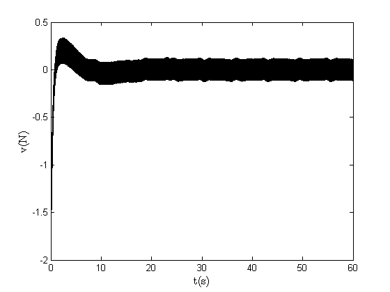
Figure 3: Control action for the discontinuous sliding mode controller.

Figure 4: Cart position (a) and pole angle (b) with the smoothed version of the sliding mode controller.

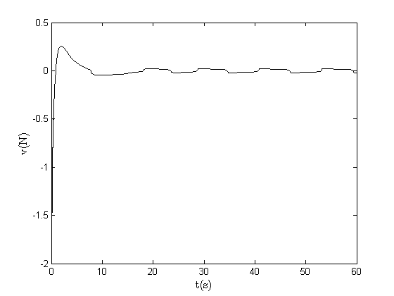
Figure 5: Control action for the smoothed version of the sliding mode controller.

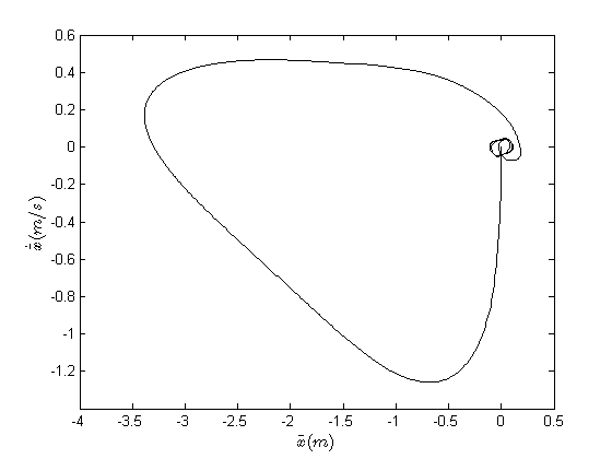
Figure 6: Phase portrait for the cart variables with the smoothed version of the sliding mode controller.

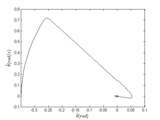
Figure 7: Phase portrait for the pole variables with the smoothed version of the sliding mode controller.

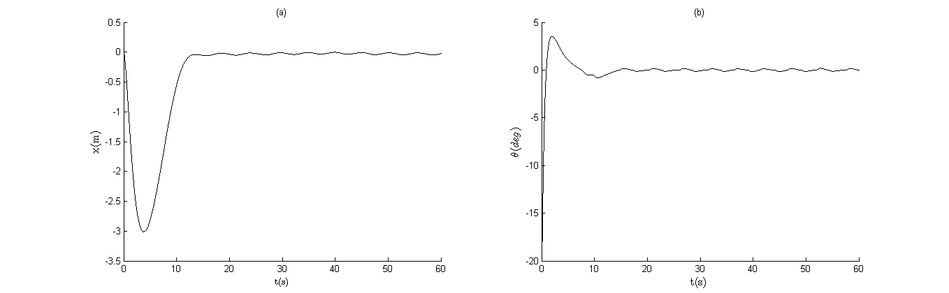
Figure 8: Cart position (a) and pole angle (b) with the intelligent sliding mode controller.

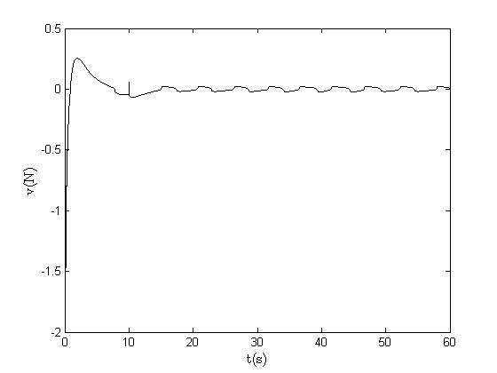
Figure 9: Control action for the intelligent sliding mode controller.

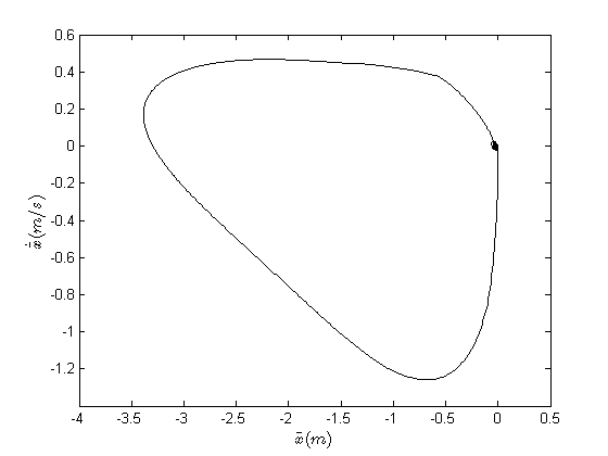
Figure 10: Phase portrait for the cart variables with the intelligent sliding mode controller.

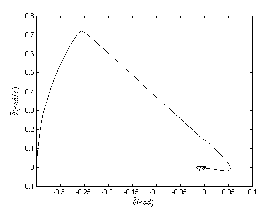
Figure 11: Phase portrait for the pole variables with the intelligent sliding mode controller.

CONCLUDING REMARKS

The present work addressed the problem of controlling uncertain nonlinear underactuated systems with a sliding mode control approach, but enhanced with a RBF neural network. The convergence properties of the resulting intelligent controller are proved by means of a Lyapunov-like stability analysis. In order to illustrate the controller design method, the proposed scheme is applied to a cart-pole system. The control system performance is confirmed by means of numerical simulations. The adoption of a RBF network provides an smaller balancing error due to its ability to compensate the performance drop caused by the change of the sign function for the saturation function.

References

- Ashrafiuon and Erwin (2008) Ashrafiuon, H. and Erwin, R.S., 2008. “Sliding mode control of underactuated multibody systems and its application to shape change control”. International Journal of Control, Vol. 81, No. 12, pp. 1849–1858. doi:10.1080/00207170801910409.
- Bessa et al. (2017) Bessa, W.M., Kreuzer, E., Lange, J., Pick, M.A. and Solowjow, E., 2017. “Design and adaptive depth control of a micro diving agent”. IEEE Robotics and Automation Letters, Vol. 2, No. 4, pp. 1871–1877. doi:10.1109/LRA.2017.2714142.
- Bessa et al. (2018) Bessa, W.M., Brinkmann, G., Duecker, D.A., Kreuzer, E. and Solowjow, E., 2018. “A biologically inspired framework for the intelligent control of mechatronic systems and its application to a micro diving agent”. Mathematical Problems in Engineering, Vol. 2018, pp. 1–16. doi:10.1155/2018/9648126.
- Bessa (2005) Bessa, W.M., 2005. Controle por Modos Deslizantes de Sistemas Dinâmicos com Zona Morta Aplicado ao Posicionamento de ROVs. Tese (D.Sc.), COPPE/UFRJ, Rio de Janeiro, Brasil.
- Bessa (2009) Bessa, W.M., 2009. “Some remarks on the boundedness and convergence properties of smooth sliding mode controllers”. International Journal of Automation and Computing, Vol. 6, No. 2, pp. 154–158. doi:10.1007/s11633-009-0154-z.
- Bessa and Barrêto (2010) Bessa, W.M. and Barrêto, R.S.S., 2010. “Adaptive fuzzy sliding mode control of uncertain nonlinear systems”. Controle & Automação, Vol. 21, No. 2, pp. 117–126. doi:10.1590/S0103-17592010000200002.
- Bessa et al. (2012) Bessa, W.M., De Paula, A.S. and Savi, M.A., 2012. “Sliding mode control with adaptive fuzzy dead-zone compensation for uncertain chaotic systems”. Nonlinear Dynamics, Vol. 70, No. 3, pp. 1989–2001. doi:10.1007/s11071-012-0591-z.
- Bessa et al. (2014) Bessa, W.M., De Paula, A.S. and Savi, M.A., 2014. “Adaptive fuzzy sliding mode control of a chaotic pendulum with noisy signals”. ZAMM-Journal of Applied Mathematics and Mechanics/Zeitschrift fur Angewandte Mathematik und Mechanik, Vol. 94, No. 3, pp. 256–263. doi:10.1002/zamm.201200214.
- Bessa et al. (2005) Bessa, W.M., Dutra, M.S. and Kreuzer, E., 2005. “Thruster dynamics compensation for the positioning of underwater robotic vehicles through a fuzzy sliding mode based approach”. In COBEM 2005 – Proceedings of the 18th International Congress of Mechanical Engineering. Ouro Preto, Brasil.
- Bessa et al. (2019) Bessa, W.M., Otto, S., Kreuzer, E. and Seifried, R., 2019. “An adaptive fuzzy sliding mode controller for uncertain underactuated mechanical systems”. Journal of Vibration and Control, Vol. 25, No. 9, pp. 1521–1535. doi:10.1177/1077546319827393.
- Bloch et al. (2000) Bloch, A.M., Leonard, N. and Marsden, J., 2000. “Controlled Lagrangians and the stabilization of mechanical systems I: The first matching theorem”. IEEE Transactions on Automatic Control, Vol. 45, No. 12, pp. 2253–2270. doi:10.1109/9.895562.
- Bloch et al. (2001) Bloch, A., Chang, D.E., Leonard, N. and Marsden, J., 2001. “Controlled Lagrangians and the stabilization of mechanical systems II: Potential shaping”. IEEE Transactions on Automatic Control, Vol. 46, No. 10, pp. 1556–1571. doi:10.1109/9.956051.
- Chen and Huang (2012) Chen, Y.F. and Huang, A.C., 2012. “Controller design for a class of underactuated mechanical systems”. IET Control Theory & Applications, Vol. 6, No. 1, pp. 103–110. doi:10.1049/iet-cta.2010.0667.
- Consolini et al. (2010) Consolini, L., Maggiore, M., Nielsen, C. and Tosques, M., 2010. “Path following for the PVTOL aircraft”. Automatica, Vol. 46, No. 8, pp. 1284–1296.
- De Macedo Fernandes et al. (2012) De Macedo Fernandes, J.M., Tanaka, M.C., Freire Júnior, R.C.S. and Bessa, W.M., 2012. “Feedback linearization with a neural network based compensation scheme”. In H. Yin, J.A. Costa and G. Barreto, eds., Intelligent Data Engineering and Automated Learning – IDEAL 2012, Springer, Vol. 7435 of Lecture Notes in Computer Science, pp. 594–601. doi:10.1007/978-3-642-32639-4˙72.
- Do and Pan (2009) Do, K. and Pan, J., 2009. Control of Ships and Underwater Vehicles: Design for Underactuated and Nonlinear Marine Systems. Advances in Industrial Control. Springer.
- Dos Santos and Bessa (2019) Dos Santos, J.D.B. and Bessa, W.M., 2019. “Intelligent control for accurate position tracking of electrohydraulic actuators”. Electronics Letters, Vol. 55, No. 2, pp. 78–80. doi:10.1049/el.2018.7218.
- Gómez-Estern and der Schaft (2004) Gómez-Estern, F. and der Schaft, A.V., 2004. “Physical damping in IDA-PBC controlled underactuated mechanical systems”. European Journal of Control, Vol. 10, No. 5, pp. 451–468. doi:10.3166/ejc.10.451-468.
- Hornik (1991) Hornik, K., 1991. “Approximation capabilities of multilayer feedforward networks”. Neural Networks, Vol. 4, No. 2, pp. 251–257.
- Lai et al. (2009) Lai, X.Z., She, J.H., Yang, S.X. and Wu, M., 2009. “Comprehensive unified control strategy for underactuated two-link manipulators”. IEEE Transactions on Systems, Man, and Cybernetics, Part B: Cybernetics, Vol. 39, No. 2, pp. 389–398.
- Lima et al. (2018) Lima, G.S., Bessa, W.M. and Trimpe, S., 2018. “Depth control of underwater robots using sliding modes and gaussian process regression”. In LARS 2018 – Proceedings of the Latin American Robotic Symposium. João Pessoa, Brazil. doi:10.1109/LARS/SBR/WRE.2018.00012.
- Lima et al. (2021) Lima, G.S., Porto, D.R., de Oliveira, A.J. and Bessa, W.M., 2021. “Intelligent control of a single-link flexible manipulator using sliding modes and artificial neural networks”. Electronics Letters, Vol. 57, No. 23, pp. 869–872. doi:10.1049/ell2.12300.
- Lima et al. (2020) Lima, G.S., Trimpe, S. and Bessa, W.M., 2020. “Sliding mode control with gaussian process regression for underwater robots”. Journal of Intelligent & Robotic Systems, Vol. 99, No. 3, pp. 487–498. doi:10.1007/s10846-019-01128-5.
- Liu and Yu (2013) Liu, Y. and Yu, H., 2013. “A survey of underactuated mechanical systems”. IET Control Theory & Applications, Vol. 7, No. 7, pp. 921–935. doi:10.1049/iet-cta.2012.0505.
- Muske et al. (2010) Muske, K.R., Ashrafiuon, H., Nersesov, S. and Nikkhah, M., 2010. “Optimal sliding mode cascade control for stabilization of underactuated nonlinear systems”. Journal of Dynamic Systems, Measurement, and Control, Vol. 134, No. 2, pp. 021020:1–11. doi:10.1115/1.4005367.
- Nguyen and Dankowicz (2015) Nguyen, K.D. and Dankowicz, H., 2015. “Adaptive control of underactuated robots with unmodeled dynamics”. Robotics and Autonomous Systems, Vol. 64, pp. 84–99. doi:10.1016/j.robot.2014.10.009.
- Ortega et al. (2002) Ortega, R., Spong, M., Gómez-Estern, F. and Blankenstein, G., 2002. “Stabilization of a class of underactuated mechanical systems via interconnection and damping assignment”. IEEE Transactions on Automatic Control, Vol. 47, No. 8, pp. 1218–1233. doi:10.1109/TAC.2002.800770.
- Park and Sandberg (1991) Park, J. and Sandberg, I.W., 1991. “Universal approximation using radial-basis-function networks”. Neural Computation, Vol. 3, No. 2, pp. 246–257.
- Pucci et al. (2015) Pucci, D., Romano, F. and Nori, F., 2015. “Collocated adaptive control of underactuated mechanical systems”. IEEE Transactions on Robotics, Vol. 31, No. 6, pp. 1527–1536. doi:10.1109/TRO.2015.2481282.
- Qian et al. (2009) Qian, D.W., Liu, X.J. and Yi, J.Q., 2009. “Robust sliding mode control for a class of underactuated systems with mismatched uncertainties”. Proceedings of the Institution of Mechanical Engineers, Part I: Journal of Systems and Control Engineering, Vol. 223, No. 6, pp. 785–795. doi:10.1243/09596518JSCE734.
- Rapp et al. (2012) Rapp, C., Kreuzer, E. and Sri Namachchivaya, N., 2012. “Reduced normal forms for nonlinear control of underactuated hoisting systems”. Archive of Applied Mechanics, Vol. 82, No. 3, pp. 297–315.
- Rudra et al. (2014) Rudra, S., Barai, R.K. and Maitra, M., 2014. “Nonlinear state feedback controller design for underactuated mechanical system: A modified block backstepping approach”. ISA Transactions, Vol. 53, No. 2, pp. 317–326. doi:10.1016/j.isatra.2013.12.021.
- Ryalat and Laila (2016) Ryalat, M. and Laila, D.S., 2016. “A simplified IDA-PBC design for underactuated mechanical systems with applications”. European Journal of Control, Vol. 27, pp. 1–16. doi:10.1016/j.ejcon.2015.12.001.
- Sankaranarayanan and Mahindrakar (2009) Sankaranarayanan, V. and Mahindrakar, A.D., 2009. “Control of a class of underactuated mechanical systems using sliding modes”. IEEE Transactions on Robotics, Vol. 25, No. 2, pp. 459–467. doi:10.1109/TRO.2008.2012338.
- Seifried (2013) Seifried, R., 2013. Dynamics of Underactuated Multibody Systems: Modeling, Control and Optimal Design. Solid Mechanics and Its Applications. Springer. doi:10.1007/978-3-319-01228-5.
- Seifried and Blajer (2013) Seifried, R. and Blajer, W., 2013. “Analysis of servo-constraint problems for underactuated multibody systems”. Mechanical Sciences, Vol. 4, No. 1, pp. 113–129.
- Seifried (2012a) Seifried, R., 2012a. “Integrated mechanical and control design of underactuated multibody systems”. Nonlinear Dynamics, Vol. 67, No. 2, pp. 1539–1557. doi:10.1007/s11071-011-0087-2.
- Seifried (2012b) Seifried, R., 2012b. “Two approaches for feedforward control and optimal design of underactuated multibody systems”. Multibody System Dynamics, Vol. 27, No. 1, pp. 75–93. doi:10.1007/s11044-011-9261-z.
- Serrano et al. (2014) Serrano, M., Scaglia, G., Godoy, S., Mut, V. and Ortiz, O., 2014. “Trajectory tracking of underactuated surface vessels: A linear algebra approach”. IEEE Transactions on Control Systems Technology, Vol. 22, No. 3, pp. 1103–1111.
- Spong (1994) Spong, M.W., 1994. “Partial feedback linearization of underactuated mechanical systems”. In IROS ’94 – Proceedings of the IEEE/RSJ/GI International Conference on Intelligent Robots and Systems. pp. 314–321. doi:10.1109/IROS.1994.407375.
- Sun et al. (2013) Sun, N., Fang, Y. and Zhang, X., 2013. “Energy coupling output feedback control of 4-DOF underactuated cranes with saturated inputs”. Automatica, Vol. 49, No. 5, pp. 1318–1325.
- Tanaka et al. (2013) Tanaka, M.C., de Macedo Fernandes, J.M. and Bessa, W.M., 2013. “Feedback linearization with fuzzy compensation for uncertain nonlinear systems”. International Journal of Computers, Communications & Control, Vol. 8, No. 5, pp. 736–743.
- Tsiotras and Luo (2000) Tsiotras, P. and Luo, J., 2000. “Control of underactuated spacecraft with bounded inputs”. Automatica, Vol. 36, No. 8, pp. 1153–1169.
- Xin and Liu (2013) Xin, X. and Liu, Y., 2013. “Reduced-order stable controllers for two-link underactuated planar robots”. Automatica, Vol. 49, No. 7, pp. 2176–2183.
- Xu and Hu (2013) Xu, L. and Hu, Q., 2013. “Output-feedback stabilisation control for a class of under-actuated mechanical systems”. IET Control Theory & Applications, Vol. 7, No. 7, pp. 985–996. doi:10.1049/iet-cta.2012.0734.
- Xu and Özgüner (2008) Xu, R. and Özgüner, Ü., 2008. “Sliding mode control of a class of underactuated systems”. Automatica, Vol. 44, No. 1, pp. 233–241. doi:10.1016/j.automatica.2007.05.014.