Compressing the chronology of a temporal network with graph commutators

Abstract

Studies of dynamics on temporal networks often represent the network as a series of “snapshots,” static networks active for short durations of time. We argue that successive snapshots can be aggregated if doing so has little effect on the overlying dynamics. We propose a method to compress network chronologies by progressively combining pairs of snapshots whose matrix commutators have the smallest dynamical effect. We apply this method to epidemic modeling on real contact tracing data and find that it allows for significant compression while remaining faithful to the epidemic dynamics.

Introduction

High resolution temporal interaction data is now simple to obtain and widely available thanks to methods such as radio frequency identification Cattuto et al. (2010) or Bluetooth signals Sapiezynski et al. (2019). Temporal interactions have rich dynamics in continuous time, yet we often want to combine intervals of temporal data into a series of simpler, static networks in order to compress the data, reduce analytical complexity, or streamline data collection efforts. For example, digital contact tracing protocols ping devices at fixed intervals to save energy and lighten data requirements. However, it is nontrivial to determine when and how to aggregate temporal data without losing critical information about the dynamics of the interactions.

Many methods currently exist to represent and analyze temporal networks Holme and Saramäki (2012), and to find patterns in network structure and dynamics. This includes algorithms for detecting temporal states Masuda and Holme (2019), dynamical approaches for generating synthetic temporal network data Peixoto and Rosvall (2017); Zhang et al. (2017), tools to identify community structure in time-varying networks Ghasemian et al. (2016), data-driven approaches to model dynamics on temporal networks by determining change points P. Peixoto and Gauvin (2018), and methods to represent key temporal features as static networks Holme (2013); Scholtes et al. (2016). The dynamics of epidemic spread on temporal networks is well-studied Rocha et al. (2011); Génois et al. (2015); Ren and Wang (2014); Valdano et al. (2015), as are synchronization Boccaletti et al. (2006); Stilwell et al. (2006); Zhang and Strogatz (2021) and control dynamics Li et al. (2017).

A continuing challenge is the interplay of dynamics on the network (changes in variables on nodes and edges) with dynamics of the network (where the topological structure changes over time). When the timescales of these two are well separated, we can take one of two limits. If the dynamics on the network are much faster, we can use a static limit where the network structure is essentially constant. When the dynamics on the network are much slower, referred to as the annealed limit, then the dynamical variables effectively experience the average of the network structure over time. Then we can aggregate many snapshots regardless of their chronological order. In between these two limits, neither type of dynamics can be neglected St-Onge et al. (2018). Then it is less clear how or if the history of the network’s structure can be compressed while remaining faithful to the dynamics on the network.

Here, we quantify the importance of chronology in a sequence of network snapshots by considering its effects on dynamics. Our goal is to compress unimportant structural changes while preserving changes that significantly affect the dynamical process. We propose a method to do so by assessing the sensitivity of the dynamics to aggregating pairs of network snapshots. We take an epidemic spreading model as our main example, but we abstract the dynamics in a way that could represent other dynamical processes on networks (e.g., synchronization of coupled oscillators or cascading failures in power grids). Specifically, we formulate a pairwise error measure using matrix commutators that captures how aggregating snapshots affects the epidemic process, and we aggregate network snapshots as long as this error remains low. Using synthetic networks and real data, we find that this approach is successful at producing a compressed snapshot sequence that still mimics the dynamic behavior of the original sequence.

Figure 1: Schema of our hierarchical aggregation. Given network snapshots, we compare the aggregate spreading dynamics of each adjacent pair of snapshots and combine the pair with the lowest induced error, continuing until we reach a desired number of snapshots.

Analytical framework

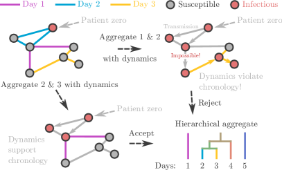
We assume that we have some temporal network data consisting of a large number of snapshots of the network structure. (If we have a series of brief contacts between pairs of nodes in continuous time, this data would consist of a large series of mostly empty graphs.) We consider the dynamical error we would introduce by aggregating a given consecutive pair of snapshots into one. In an epidemic model, this error consists of creating paths that allow the contagion to progress backwards in time, as depicted in Fig. 1. If aggregating two snapshots would create many such chronology-violating paths, we should keep these snapshots separate and respect their chronological order.

In our epidemic example, a contagion spreads along edges connecting infectious nodes to their susceptible neighbors. We measure the effect of pairwise aggregation with a measure of error capturing the difference in the number of infected individuals, with and without aggregation over the duration of the snapshot pair. As we will see, we can approximate this error in terms of the commutator of two matrices, each of which linearizes the dynamics over the time interval of the snapshots.

Linearizing the SI model

Let $A(t)$ be the time-varying adjacency matrix of a network with $N$ nodes. Let $P(t)$ be a vector of length $N$ where $P_{i}(t)$ is the probability that a node $i$ is infected at time $t$. A susceptible-infected-susceptible (SIS) model with infection rate $\beta$ and recovery rate $\gamma$ can be modeled by the following system of differential equations:

$$\frac{dP_{i}}{dt}=\beta\big{(}1-P_{i}(t)\big{)}\big{(}A(t)\cdot P(t)\big{)}_{i}-\gamma P_{i}\,,$$ (1)

and the total number of infected individuals at time $t$ is $I(t)=|P(t)|$ where $|P|=\sum_{i=1}^{N}P_{i}$. In this paper we will focus on the SI model where $\gamma=0$. We then consider the early time linearization of Eq. (1) around $P=0$ (without losing much accuracy sup ), and thus have

$$\frac{dP}{dt}=\beta A(t)P(t)\,.$$ (2)

The solution to this equation involves a time-ordered exponential of $A(t)$. In the case of a series of snapshots $A_{1},\ldots,A_{\ell}$, i.e., a sequence of static adjacency matrices which hold over time intervals of duration $\delta t_{1},\ldots,\delta t_{\ell}$, we have

$$P(t)=\left[\prod_{i=\ell}^{1}\exp\left(\beta\delta t_{i}A_{i}\right)\right]P(0)$$ (3)

(This product is in reverse order since we treat $P(t)$ as a column vector and multiply on the left.) If all the $A_{i}$ commute, this product reduces to $\exp\left(\beta\sum_{i}\delta t_{i}A_{i}\right)$, a single exponential of their weighted average. However, in general their noncommutative nature must be taken into account.

Figure 2: Top left: Degree distributions for two snapshots. Top right: ordinary differential equation solutions of the SI dynamics with $\beta=0.12$, $\delta t=5$ on the temporal and aggregate versions of the snapshots. Bottom left: ODE solution difference in number of infected nodes under the temporal and aggregate regimes for varying values of $\beta t$ by varying $t=[0,5]$. Bottom right: Ranking of $\xi_{1,2}$ for snapshots 1 and 2 for increasing values of $\beta\delta_{t}$ compared against the integrated area between solutions.

Aggregating snapshots

Say we have two consecutive snapshots, $A$ and $B$, which are valid for time intervals $[t^{A}_{0},t^{A}_{1}]$ and $[t^{B}_{0},t^{B}_{1}]$ of duration $\delta t_{A}=t^{A}_{1}-t^{A}_{0}$ and $\delta t_{B}=t^{B}_{1}-t^{B}_{0}$ respectively, where $t^{B}_{0}=t^{A}_{1}$. In the linearized SI dynamics of Eq. (2), aggregating $A$ and $B$ in a single step is equivalent to replacing the time evolution operator $\exp(\beta\delta t_{B}B)\exp(\beta\delta t_{A}A)$ with

$$\exp\big{(}\beta(\delta t_{A}+\delta t_{B})\overline{(A,B)}\big{)}\,,$$

where $\overline{(A,B)}$ is the time-weighted average

$$\overline{(A,B)}=\frac{\delta t_{A}A+\delta t_{B}B}{\delta t_{A}+\delta t_{B}}\,.$$ (4)

We can quantify of the effect of this aggregation using the Baker-Campbell-Hausdorff formula, which expresses the product $\exp X\exp Y$ as a single exponential $\exp Z$:

$$Z=X+Y+\frac{1}{2}[X,Y]+\frac{1}{12}\big{(}[X,[X,Y]]]-[Y,[X,Y]]\big{)}+\cdots$$ (5)

where $[X,Y]=XY-YX$ is the matrix commutator. Setting $X=\beta\delta t_{B}B$ and $Y=\beta\delta t_{A}A$, we have

$$\exp(\beta\delta_{B}B)\,\exp(\beta\delta_{A}A)=\exp Z\,,$$

where

$$Z=\beta(\delta t_{A}+\delta t_{B})\overline{(A,B)}+\frac{1}{2}\,\beta^{2}\delta t_{A}\delta t_{B}\left[B,A\right]+O(\beta^{3})\;.$$ (6)

The correction term proportional to $[B,A]$ shows to leading order how aggregation introduces error into the dynamics. As illustrated in Fig. 1, aggregation creates chronology-violating paths whenever $A$ and $B$ do not commute. For example, if $A$ includes the edge $(1,2)$ and $B$ includes the edge $(2,3)$, then a disease could spread from node 1 to 3 in the chronology $BA$ but not in $AB$. The commutator $[B,A]$ counts paths allowed by $BA$ and subtracts paths allowed by $AB$, compensating for the fact that the Taylor series of $\exp(\overline{(A,B)})$ contains terms proportional to both $AB$ and $BA$.

Thus we use the correction term in Eq. (6) as a measure of the error induced by aggregation, or equivalently a measure of the sensitivity of the dynamics to the temporal ordering of $A$ and $B$. Specifically, we use the operator norm of this term, i.e., its largest singular value, as an estimate of the error induced from the start to the end of the combined interval $[t_{0}^{A},t_{1}^{B}]$:

$$\epsilon_{\textrm{END}}=\frac{1}{2}\,\beta^{2}\delta t_{A}\delta t_{B}\|[B,A]\|_{\textrm{op}}$$ (7)

The operator norm bounds the effect of aggregation on any state $P(t_{0}^{A})$ at the beginning of the interval. Note that $\epsilon_{\textrm{END}}$ is small if $\beta$ is small, i.e., if the epidemic dynamics is slow compared to the dynamics of the network structure. It is also small if either $\delta t_{A}$ or $\delta t_{B}$ is small, since in that case the effect of $A$ or $B$ is close to the identity.

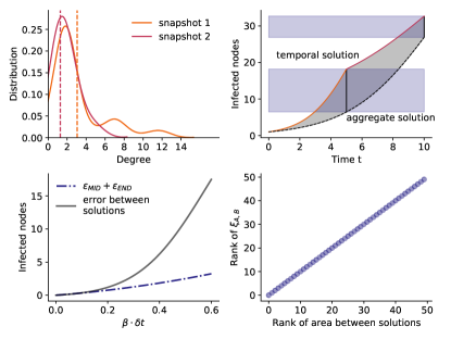
As shown in Fig. 2, we are interested in the effect of aggregation on the entire history of the system, not just the final state. Thus we also consider the error induced at the boundary $t_{1}^{A}=t_{0}^{B}$ between the two intervals. To leading order we have

$$\exp(\beta\delta t_{A}A)-\exp\!\left(\beta\delta t_{A}\overline{(A,B)}\right)=\beta\delta t_{A}\left(A-\overline{(A,B)}\right)+O(\beta^{2})\,.$$

This term is in fact symmetric in $A$ and $B$, since

$$\beta\delta t_{A}\left(A-\overline{(A,B)}\right)=\beta\frac{\delta t_{A}\delta t_{B}}{\delta t_{A}+\delta t_{B}}(A-B)\,.$$

As before we bound the possible error induced at the midpoint as the operator norm of this term,

$$\epsilon_{\textrm{MID}}=\beta\frac{\delta t_{A}\delta t_{B}}{\delta t_{A}+\delta t_{B}}\|A-B\|_{\textrm{op}}\,.$$ (8)

We scale these terms by the cumulative duration of both snapshots—capturing the total effect that $\epsilon_{\textrm{MID}}$ and $\epsilon_{\textrm{END}}$ have on the epidemic process (as visualized in the top right panel of Fig. 2)—which culminates in our error measure defined as

$$\xi_{A,B}=(\epsilon_{\textrm{END}}+\epsilon_{\textrm{MID}})(\delta t_{A}+\delta t_{B}).$$ (9)

This measure includes both the error incurred by the overall difference between $A$ and $B$, and the extent to which their chronological order matters. If our main goal is to compute the final state, we can place a smaller weight on $\epsilon_{\textrm{MID}}$ or focus entirely on $\epsilon_{\textrm{END}}$. Note that while $\epsilon_{\textrm{END}}$ is second order in $\beta$ and $\epsilon_{\textrm{MID}}$ is first order, either can dominate, e.g., if $A$ and $B$ have average degree $d$ then $\|[A,B]\|_{\textrm{op}}$ can grow as $d^{2}$.

Compression Algorithm

Given a temporal network dataset as a sequence of $M$ snapshots, we can use the framework to compress the snapshots into $M-j$ snapshots via a greedy algorithm. First, the number of desired iterations $j$ is set. For steps from 1 to $j$,

1. Compute the error $\xi_{A,B}$ from Eq. (9) for each ordered pair $A,B$ of consecutive snapshots.

2. Identify the pair $A^{*},B^{*}=\text{argmin}_{A,B}(\xi_{A,B})$ to compress.

3. Replace $A$ and $B$ with with their aggregate, $(\overline{(A,B)}$ over the union $[t_{0}^{A},t_{1}^{B}]$ of their time intervals.

Alternately, we can compress until $\min_{A,B}\xi_{A,B}$ reaches some threshold.

This algorithm produces a hierarchical aggregation of snapshots as portrayed in Fig. 1. Periods where the network structure changes slowly or where snapshots commute become single snapshots with a long duration, while the periods with rapidly changing and noncommuting structures are preserved at a higher temporal resolution.

Figure 3: Algorithm run on a series of 50 synthetic network snapshots (detailed in appendix sup ), showing the SI dynamics with $\beta=0.0017$ and intervals of width $\delta t=5$. Top: we use our algorithm to compress the network history to $6$ snapshots of varying lengths, with boundaries shown by the blue dashed lines. We compare with the SI dynamics using even-width aggregation into $6$ windows of fixed length (yellow dashed lines). The snapshots produced by our algorithm give SI dynamics closer to that on the full temporal network (gray) than the even-width approach. Middle: normalized distance from the temporal curve over time for each solution, $d_{\textrm{ALG}}$ for the algorithmic solution, and $d_{\textrm{EVEN}}$ for the even-wdith solution. Bottom: shows the shaded area from the middle panel as a function of number of aggregated snapshots, as a fraction of the error induced by aggregating the entire history into a single static network. For a given number of snapshots, our algorithm achieves and error roughly one tenth of that achieved by dividing the history evenly into time windows of equal length.

Results

Our algorithm produces aggregated snapshots that are able to better support the epidemic dynamics on the temporal network than the standard approach of evenly dividing time into windows of some fixed length and aggregating snapshots in each window. To show this, we integrate the SI dynamics of Eq. (1) using the full temporal dataset, $x(t)_{\textrm{TEMP}}$, as well as over evenly-divided aggregated snapshots, $x(t)_{\textrm{EVEN}}$, and the snapshots produced by our algorithm, $x(t)_{\textrm{ALG}}$. We measure the multiplicative error $d_{\textrm{EVEN}}$ as

$$d_{\textrm{EVEN}}=\int\frac{|x(t)_{\textrm{EVEN}}-x(t)_{\textrm{TEMP}}|}{x(t)_{\textrm{TEMP}}}dt$$ (10)

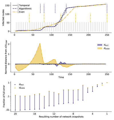
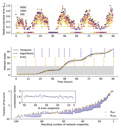
and similarly for $d_{\textrm{EVEN}}$. We apply the algorithm to synthetic networks in Fig. 3, and to a dataset of four days and nights of contacts in a hospital in Fig. 4 Vanhems et al. (2013).

We show in the top panel of Fig. 4 how the sensitivity of certain temporal ranges is maintained over a large range of resolution, which allows for pre-aggregation of data to improve the speed of the algorithm. The error metric also allows us to identify the daily patterns of the contact data at a glance. Once integrated in the compression algorithm, the middle panel shows how we can aggregate over nights at the hospital, and capture the daily activity in one or two snapshots. As seen in the bottom panels of Fig. 3 and Fig. 4, our algorithm compresses more effectively than even-width time windows: for a given number of even-width aggregation steps, the algorithm can attain the same level of error after significantly more aggregation steps due to the systematic way the snapshots pairs are chosen.

Figure 4: Application to a hospital contact network Vanhems et al. (2013). Top: the error measure $\xi_{S(t),S(t+1)}$ computed for consecutive snapshot pairs at 3 different levels of pre-aggregation. The hospital contact data contains contacts for approximately $9,000$ unique timestamps. We pre-aggregate by evenly coarse-graining the data to 4,000, 1,000 and 200 snapshots. Pre-aggregation of the data into small static snapshots does not affect the overall quality of our compression sup . Middle: the compression algorithm run on a the 200 snapshots to generate $10$ snapshots, compared to the fully temporal dynamics and the dynamics under even compression. The 200 pre-aggregated snapshots each have duration $1737$ seconds with mean $27.34$ contacts per snapshot. We used a $\beta=0.000015$ such that $\beta\delta_{t}\in[0.025,0.5]$. The parameters $\beta\delta t$ are not sensitive, as long as they do not lead to immediate saturation of the network sup . Vertical lines show boundaries for the resulting aggregated snapshots. Bottom: shows the error of the SI process solutions from the middle panel as a function of resulting number of aggregated snapshots, relative to the error induced by aggregating the entire history as a single static network. The vertical axis of the inset shows the ratio of compression achieved by our algorithm versus even-width aggregation, while maintaining a lower or equivalent level of error than the given level of even-width compression on the horizontal axis. For example, our algorithm can perform 48 snapshot compressions while maintaining lower error than that of 30 snapshot compressions of even width. Our algorithm can, on average, further compress the number of snapshots by over 60% while preserving the error induced on the resulting dynamics.

Discussion

The measure $\xi_{A,B}$ of the error induced by aggregating adjacent snapshots, and our hierarchical compression algorithm based on it, offer at least four interesting applications.

First, the approach can directly provide bounds of accuracy when studying dynamics on temporal networks with tools developed for spreading on static networks. Second, our algorithm can help compress large sequences of temporal networks by aggregating consecutive pairs of networks to reach a desired level of simplification. Our algorithm could also be modified to aggregate snapshots until the expected error caused by this aggregation is smaller than some threshold. As shown in Fig. 4 using real temporal interaction data, this approach allowed us to consistently meet a certain level of error while decreasing the number of required network snapshots almost by half compared to aggregating into even-width windows.

Third, the error can be used to estimate the accuracy of data collection in the first place by testing how compressible the data might be. This could help focus data collection efforts by identifying places and times with fast temporal variations, as in the top panel of Fig. 4. Fourth, the error can be used on non-temporal data to compare the structure of any two networks that share some of the same nodes and support the same dynamics. At its core, our approach is a network comparison tool: How different are dynamics on two networks compared to dynamics on their average?

One important limitation is the greediness of our algorithm, as it can get stuck in sub-optimal compression sequences. Future work should also explore how to predict the optimal stopping point of temporal compression. Altogether, we hope that our work will inspire more tools to compress temporal network data which is an area rich in possible applications.

References

- Cattuto et al. (2010) C. Cattuto, W. Van den Broeck, A. Barrat, V. Colizza, J.-F. Pinton, and A. Vespignani, PloS ONE 5, e11596 (2010).
- Sapiezynski et al. (2019) P. Sapiezynski, A. Stopczynski, D. D. Lassen, and S. Lehmann, Scientific Data 6, 1 (2019).
- Holme and Saramäki (2012) P. Holme and J. Saramäki, Physics Reports 519, 97 (2012).
- Masuda and Holme (2019) N. Masuda and P. Holme, Scientific Reports 9, 795 (2019).
- Peixoto and Rosvall (2017) T. P. Peixoto and M. Rosvall, Nature Communications 8, 582 (2017).
- Zhang et al. (2017) X. Zhang, C. Moore, and M. E. J. Newman, The European Physical Journal B 90, 200 (2017).
- Ghasemian et al. (2016) A. Ghasemian, P. Zhang, A. Clauset, C. Moore, and L. Peel, Physical Review X 6, 031005 (2016), publisher: American Physical Society.
- P. Peixoto and Gauvin (2018) T. P. Peixoto and L. Gauvin, Scientific Reports 8, 15511 (2018).
- Holme (2013) P. Holme, PLoS Computational Biology 9 (2013), https://doi.org/10.1371/journal.pcbi.1003142.
- Scholtes et al. (2016) I. Scholtes, N. Wider, and A. Garas, The European Physical Journal B 89, 61 (2016).
- Rocha et al. (2011) L. E. C. Rocha, F. Liljeros, and P. Holme, PLoS Computational Biology 7 (2011), https://doi.org/10.1371/journal.pcbi.1001109.
- Génois et al. (2015) M. Génois, C. L. Vestergaard, C. Cattuto, and A. Barrat, Nature Communications 6, 8860 (2015).
- Ren and Wang (2014) G. Ren and X. Wang, Chaos 24, 023116 (2014), publisher: American Institute of Physics.
- Valdano et al. (2015) E. Valdano, L. Ferreri, C. Poletto, and V. Colizza, Physical Review X 5, 021005 (2015), publisher: American Physical Society.
- Boccaletti et al. (2006) S. Boccaletti, D.-U. Hwang, M. Chavez, A. Amann, J. Kurths, and L. M. Pecora, Physical Review E 74, 016102 (2006).
- Stilwell et al. (2006) D. J. Stilwell, E. M. Bollt, and D. G. Roberson, SIAM Journal on Applied Dynamical Systems 5, 140 (2006).
- Zhang and Strogatz (2021) Y. Zhang and S. H. Strogatz, Nature Communications 12, 1 (2021).
- Li et al. (2017) A. Li, S. P. Cornelius, Y.-Y. Liu, L. Wang, and A.-L. Barabási, Science 358, 1042 (2017).
- St-Onge et al. (2018) G. St-Onge, J.-G. Young, E. Laurence, C. Murphy, and L. J. Dubé, Phys. Rev. E 97, 022305 (2018).
- (20) See Supplemental Material for further detail on our derivation of the error measure, on our algorithmic implementation, and on our experiments.
- Vanhems et al. (2013) P. Vanhems, A. Barrat, C. Cattuto, J.-F. Pinton, N. Khanafer, C. Régis, B.-a. Kim, B. Comte, and N. Voirin, PLoS ONE 8, e73970 (2013).